Zombie Compositions in Assembly Algebras
and an Upper Bound on the Size of Chemical Space
January 01, 1970
Abstract
In this paper we present construction systems—tuples \((X, \mathrm{BB}, \oplus, \nu)\) comprising objects, building blocks, an assembly operation, and a joining multiplicity—as a general algebraic framework for studying how complex objects are built from simpler parts. To each construction system we associate a toric ideal, a toric variety, and a matroid, obtaining analytical bounds on the growth function \(N(a)\) (the number of objects of construction complexity \(\leq a\)) purely from the design signature \((m, \nu, n_0)\).
For systems equipped with a type system and valence bounds, we define the composition polytope \(P_{\mathrm{val}} \subset \mathbb{R}^m\), whose integer points count the feasible compositions. Compositions outside \(P_{\mathrm{val}}\)—termed zombies—are combinatorially valid but physically unrealisable. We prove that the zombie classification is sound (zero false positives) and conservative: the true infeasibility rate is at least as high as the polytope predicts.
Specialising to the molecular graph assembly system of Morales Parra et al.(\(m = 19\) bond types, \(5\) atom types with valences \(1\)–\(4\)), we identify a composition polytope whose lattice points capture the physically realisable compositions, and show that the resulting growth exponent tightens from \(0.73\) to the exact value \(\log 2 \approx 0.693\). While the difference of \(0.037\) appears small, in the doubly-exponential regime it corresponds to a tightening of the bound by a factor exceeding \(10^{198}\) at assembly index \(10\). The framework also recovers the bioorthogonal click-chemistry system of the author’s prior work as a second instance, with \(m = 8\) and a partition matroid.
1 Introduction↩︎
The question of how the number of constructible objects grows with construction complexity arises in diverse domains: molecular chemistry, where one asks how many molecules can be assembled from a given set of bond types; combinatorial design, where one counts the structures buildable from specified components; and circuit complexity, where analogous questions arise for Boolean functions.
Recently, Morales Parra et al.[1] addressed this question for molecular graphs, extending Assembly Theory [2], [3] into a framework for estimating the size of chemical space. Their central result is a doubly-exponential upper bound on the growth function \(N(a)\)—the number of molecules with assembly index at most \(a\)—with a fitted exponent of approximately \(0.73\).In this paper we develop a purely algebraic framework that subsumes Assembly Theory and shows that this estimate overestimates the size of chemical space. The starting point is not chemistry but algebra: given a set-valued binary operation \(\oplus\) on a countable set \(X\) with a finite set of building blocks \(\mathrm{BB}\), what is the algebraic structure of the space of constructible objects? How does it grow with construction complexity? How does it transform under constraints?
We answer these questions by introducing construction systems (Definition 1)—tuples \((X, \mathrm{BB}, \oplus, \nu)\) parametrised by a design signature \((m, \nu, n_0)\)—and showing that the assembly process naturally gives rise to a toric ideal \(I_A\) (Definition 5), a toric variety \(X_A\), and a matroid \(M\) (Definition 9). The machinery of toric geometry—as developed in Sturmfels [4], Fulton [5], and Cox–Little–O’Shea [6]—provides the algebraic infrastructure; the analytical bounds on \(N(a)\) follow from the combinatorics of these objects alone, without reference to any specific chemical or physical system.
Our main contributions are as follows.
(i) General algebraic framework (§2–3). Construction systems yield toric ideals, toric varieties, and matroids. The “rules” of any concrete system—chemical, physical, or logical—are not external constraints imposed on a pre-existing space; they are the toric ideal. Constraints on the building blocks correspond to matroid operations (restriction, deletion) on the block matroid \(M^*\) (Theorem 1).
(ii) Analytical bounds and the exact exponent (§4). Upper and lower bounds on \(N(a)\) depend only on the design signature \((m, \nu, n_0)\) and the matroid rank \(r\), not on any enumerated database. The doubly-exponential growth exponent is \(\rho = \log 2\) exactly (Theorem 4): the upper bound from Corollary 1 is matched by a lower bound from counting trees via Pólya enumeration.
(iii) The composition polytope and zombie exclusion (§6). For construction systems with typed building blocks and valence bounds, the composition polytope \(P_{\mathrm{val}} \subset \mathbb{R}^m\) captures all feasibility constraints in a single linear inequality. Compositions outside \(P_{\mathrm{val}}\) are zombies: combinatorially valid but physically impossible. We prove the classification is sound—zero false positives (Lemma 1)—and that it is conservative: every unmodelled constraint (pair multiplicity, degree-sequence realizability, full connectivity) can only increase the zombie fraction (Remark 21).
(iv) Refined upper bound (Theorem 6). Replacing the naïve stars-and-bars count \(\binom{S+m-1}{m-1}\) with the Ehrhart count \(E_P(S)\) of the composition polytope yields a strictly tighter growth bound. For the molecular graph system of Morales Parra et al.(\(m = 19\)), the zombie fraction reaches \(z_\infty = 94\%\) asymptotically (Corollary 5), and the exact doubly-exponential growth exponent is \(\log 2 \approx 0.693\) (Theorem 4).
(v) Concrete instances (§5). Morales Parra et al.’s molecular graph assembly and the bioorthogonal click-chemistry system of [7] emerge as corollaries by specialising three parameters.
The paper is structured as follows. Section 2 defines construction systems and their toric geometry. Section 3 develops the toric and block matroids. Section 4 derives the analytical bounds on \(N(a)\). Section 5 specialises to two concrete instances. Section 6 introduces the composition polytope, proves soundness of the zombie classification, and derives the refined bound. Section 7 presents the full computational results: zombie-generator coefficients, exact zombie fractions, and a quantitative comparison of the two upper bounds. Section 8 discusses further algebraic structure. Section 9 interprets the results in the broader context of chemical space estimation, and Section 10 summarises the main findings and identifies open questions.
2 Construction Systems and Their Toric Geometry↩︎
Definition 1 (Construction System). A construction system is a tuple \(\mathcal{S} = (X, \mathrm{BB}, \oplus, \nu)\) where:
\(X\) is a countable set of objects;
\(\mathrm{BB}\subset X\) is a finite set of building blocks, \(|\mathrm{BB}| = m\);
\(\oplus: X \times X \to \mathcal{P}(X)\) is a set-valued assembly operation;
\(\nu: \mathbb{N}\times \mathbb{N}\to \mathbb{N}\) is the joining multiplicity: \(\nu(n_1, n_2)\) is the number of distinct joinings of objects with \(n_1\) and \(n_2\) constituent parts.
The triple \((m, \nu, n_0)\), where \(n_0\) is the part-count of a single building block, is called the design signature of \(\mathcal{S}\).
Definition 2 (Assembly Tree and Construction Complexity). An assembly tree for \(O \in X\) is a rooted binary tree \(T\) whose leaves are labelled by elements of \(\mathrm{BB}\) and whose internal nodes are labelled by the result of \(\oplus\) applied to the children. The construction complexity is \[\mathop{\mathrm{AI}}(O) \;=\; \min\bigl\{\,\mathrm{depth}(T) : T \text{ is an assembly tree for } O\,\bigr\}.\]
Definition 3 (Composition Morphism). The composition morphism is \[\pi: X \longrightarrow \mathbb{N}^m, \qquad O \longmapsto \alpha(O) = (\alpha_1, \ldots, \alpha_m),\] where \(\alpha_i\) counts occurrences of building block \(b_i\) in \(O\). The total size is \(S(O) = |\alpha(O)| = \sum_i \alpha_i\).
Definition 4 (Composition Matrix). Let \(\mathcal{X} = \{O_1, \ldots, O_N\}\) be a finite ensemble of constructible objects. The composition matrix is \[A \;=\; \bigl[\,\alpha(O_1) \mid \cdots \mid \alpha(O_N)\,\bigr] \;\in\; \mathbb{N}^{m \times N}.\]
Definition 5 (Assembly Toric Ideal). The assembly toric ideal is the kernel of the monomial map (cf. [4], Ch. 4; [6], Ch. 8; [5], §1.1) \[\varphi: k[t_1, \ldots, t_N] \longrightarrow k[x_1, \ldots, x_m], \qquad t_j \longmapsto x^{\alpha(O_j)} = x_1^{\alpha_{1j}} \cdots x_m^{\alpha_{mj}}.\] That is, \(I_A = \ker(\varphi) = \langle\, t^u - t^v : Au = Av,\; u, v \in \mathbb{N}^N \,\rangle\).
The associated assembly toric variety is \(X_A = \mathbf{V}(I_A) \subset \mathbb{A}^N\) (see [5] and [6], Ch. 4).
Remark 6. The toric ideal \(I_A\) encodes all algebraic relations between compositions. This is the standard toric correspondence: every binomial \(t^u - t^v \in I_A\) witnesses a pair of objects with identical composition but distinct assembly (cf. [4]; [8], Ch. 1). In any concrete construction system, the “rules” (chemical, physical, logical) that govern which objects exist are not external constraints imposed on a pre-existing space. They are the toric ideal. The relations \(t^u - t^v\) capture precisely which sets of objects have the same total composition, i.e., use the same building blocks in the same multiplicities but combine them differently.
Definition 7 (Fiber and Its Stratification). The fiber over \(\alpha \in \mathbb{N}^m\) is \(\mathrm{Fib}(\alpha) = \pi^{-1}(\alpha)\). It decomposes by complexity: \[\mathrm{Fib}(\alpha) \;=\; \bigsqcup_{a \geq 0} \mathrm{Fib}_a(\alpha), \qquad \mathrm{Fib}_a(\alpha) = \bigl\{\, O \in \mathrm{Fib}(\alpha) : \mathop{\mathrm{AI}}(O) = a \,\bigr\}.\]
Definition 8 (Growth Function). The growth function of \(\mathcal{S}\) is \[N(a) \;=\; \bigl|\bigl\{\, O \in X : \mathop{\mathrm{AI}}(O) \leq a \,\bigr\}\bigr| \;=\; \sum_{\substack{\alpha \in \mathbb{N}^m \\ \mathrm{Fib}_{\leq a}(\alpha) \neq \varnothing}} \bigl|\mathrm{Fib}_{\leq a}(\alpha)\bigr|.\]
3 The Toric Matroid↩︎
Definition 9 (Toric Matroid). The toric matroid \(M(\mathcal{S})\) of a construction system \(\mathcal{S}\) is the linear matroid (cf. [9]) on the columns of \(A\) over \(\mathbb{Q}\): \[S \subseteq [N] \text{ is independent} \;\iff\; \{\alpha(O_j) : j \in S\} \text{ is linearly independent over } \mathbb{Q}.\] Its rank is \(r = r(M) = \mathop{\mathrm{rank}}_\mathbb{Q}(A) \leq m\).
Remark 10. The rank \(r\) has a precise semantic: it is the number of algebraically independent building-block coordinates on the toric variety \(X_A\). Equivalently, \(m - r\) is the number of independent algebraic relations (“rules”) among the building blocks, i.e., the dimension of the kernel of the composition matrix (cf. [8], §1.6; [5], §1.3). This is the toric encoding of what, in any concrete domain, would be called the “design rules” of the system.
Definition 11 (Dual Matroid on Building Blocks). The block matroid \(M^*(\mathcal{S})\) is the linear matroid on the rows of \(A\) (i.e., on \(\mathrm{BB}\)): \[B \subseteq \mathrm{BB}\text{ is independent} \;\iff\; \text{the rows of } A \text{ indexed by } B \text{ are linearly independent.}\] Its rank \(r^* = \mathop{\mathrm{rank}}_\mathbb{Q}(A) = r\) equals the rank of \(M\). A circuit of \(M^*\) is a minimal set of building blocks with a linear dependence — i.e., a minimal “rule.”
Theorem 1 (Constraints as Matroid Operations). Let \(\mathcal{S}' = (X', \mathrm{BB}' \subseteq \mathrm{BB}, \oplus, \nu)\) be a construction system obtained from \(\mathcal{S}\) by restricting the building blocks to a subset \(\mathrm{BB}' \subseteq \mathrm{BB}\). Then:
The toric matroid of \(\mathcal{S}'\) is the restriction \(M^*|_{\mathrm{BB}'}\).
Its rank satisfies \(r(\mathcal{S}') = r(M^*|_{\mathrm{BB}'}) \leq r(\mathcal{S})\), with equality iff \(\mathrm{BB}\setminus \mathrm{BB}'\) contains no coloop of \(M^*\).
Every constraint of the form “exclude building block types \(B\)” corresponds to a deletion \(M^* \setminus B\) in the block matroid.
Proof. Deleting rows of \(A\) corresponding to \(\mathrm{BB}\setminus \mathrm{BB}'\) gives the submatrix \(A'\). Linear independence of rows of \(A'\) is the restriction of the row matroid to \(\mathrm{BB}'\). A coloop of \(M^*\) is a row not in the span of the others; deleting it reduces rank by one. ◻
4 Analytical Bounds on the Growth Function↩︎
All bounds in this section depend exclusively on the design signature \((m, \nu, n_0)\) and the matroid rank \(r\). No enumerated database is used.
Proposition 12 (Individual Complexity Bounds). For any object \(O\) with \(S(O) = S\), \[\lceil\log_2 S\rceil \;\leq\; \mathop{\mathrm{AI}}(O) \;\leq\; S - 1.\]
Proof. An assembly tree of depth \(d\) has \(\leq 2^d\) leaves, so \(S \leq 2^{\mathop{\mathrm{AI}}(O)}\). Sequential unit addition achieves \(S - 1\). ◻
Theorem 2 (Lower Bound). \[N(a) \;\geq\; m \cdot \prod_{i=1}^{a} \nu(n_{i-1}, n_{i-1}), \qquad n_i = 2n_{i-1} - 1.\] In particular, if \(\nu(n, n) \geq n^2\) (vertex-identification joinings), then \[\log N(a) \;\geq\; a^2 \log 2 + O(a).\]
Proof. Fix \(b_j \in \mathrm{BB}\). Construct by recursive self-joining (doubling). At step \(i\), there are \(\geq \nu(n_{i-1}, n_{i-1})\) joinings, and the result has \(n_i = 2n_{i-1}-1\) parts. The product over \(a\) steps counts labelled assembly paths; the bound holds a fortiori for isomorphism classes. The factor \(m\) accounts for the choice of building block. Under the vertex-identification model, \(\nu(n,n) = n^2\) and \(n_i = 2^i + 1\), giving \(\prod_{i=1}^a (2^{i-1}+1)^2 \geq 2^{a(a-1)}\). ◻
Theorem 3 (Upper Bound). Let \(g(S)\) denote the number of objects realisable with \(S\) building block instances. If \(g(S) \leq \gamma^S\) for a constant \(\gamma = \gamma(\mathcal{S})\), then \[\log N(a) \;\leq\; 2^a \cdot \log(m\gamma) + O(m \log 2^a).\]
Proof. \(\mathop{\mathrm{AI}}(O) \leq a \Rightarrow S(O) \leq 2^a\). Stars-and-bars gives \(\binom{S+m-1}{m-1}\) compositions of size \(S\) into \(m\) types. Summing \(\binom{S+m-1}{m-1}\gamma^S\) over \(S = 1, \ldots, 2^a\) yields the bound. ◻
Remark 13. The constant \(\gamma\) is a design parameter: it is determined by the assembly operation \(\oplus\) and the implicit constraints of the construction system. For molecular graphs with valence constraints, \(\gamma\) can be computed from Pólya enumeration of connected graphs with prescribed degree bounds. It is not fitted from a database.
Corollary 1 (Growth Exponent). The growth exponent \[\rho \;=\; \limsup_{a \to \infty} \frac{\log \log N(a)}{a}\] satisfies \(0 < \rho \leq \log 2\). Equality \(\rho = \log 2\) holds iff the growth is doubly exponential.
Theorem 4 (Exact Growth Exponent). Let \(\mathcal{S}\) be a construction system with vertex-identification joining (\(\nu(n_1,n_2) = n_1 n_2\), \(n_0 = 2\)). If the fibre over some efficient composition grows exponentially—i.e., there exist a composition sequence \(\alpha_S\) with \(\sum_i c_i (\alpha_S)_i < 0\) for all \(S\) and a constant \(\gamma_{\min} > 1\) such that \(|\mathrm{Fib}(\alpha_S)| \geq \gamma_{\min}^S\) for all large \(S\)—then \(\rho = \log 2\).
Proof. The upper bound \(\rho \leq \log 2\) is Corollary 1. For the lower bound, note that every connected graph \(G\) with \(S\) edges admits an assembly tree of depth at most \(\lceil \log_2 S \rceil + O(1)\): the centroid decomposition splits \(G\) into components of size \(\leq S/2\), which are reassembled in a balanced binary tree of \(O(\log S)\) levels. Hence \(\mathop{\mathrm{AI}}(G) \leq \lceil\log_2 S\rceil + C\) for an absolute constant \(C\). Setting \(S = 2^{a - C}\): \[N(a) \;\geq\; |\mathrm{Fib}(\alpha_{2^{a-C}})| \;\geq\; \gamma_{\min}^{\,2^{a-C}}.\] Therefore \(\log\log N(a) \geq (a - C)\log 2 + \log\log\gamma_{\min}\), and \(\rho \geq \log 2\). ◻
Corollary 2 (Molecular Graphs). For the molecular graph assembly system with \(m = 19\) bond types, \(\rho = \log 2 \approx 0.693\).
Proof. Take \(\alpha_S = (S, 0, \ldots, 0)\) (all C–C single bonds), which has \(c_1 = -1/2 < 0\) and is valence-feasible for all \(S\). The fibre \(\mathrm{Fib}(\alpha_S)\) includes all unlabelled trees on \(S + 1\) vertices with maximum degree \(4\). By Pólya’s enumeration theorem (see [10], Ch. VII), their count satisfies \(T_4(S+1) \sim c\,\gamma^{S+1} S^{-5/2}\) with \(\gamma \approx 2.48 > 1\). The centroid of a tree with max degree \(4\) has at most \(4\) subtrees, each of size \(\leq S/2\); pairing and assembling them yields \(\mathop{\mathrm{AI}}(T) \leq \lceil\log_2 S\rceil + 2\) for every such tree. Theorem 4 applies with \(\gamma_{\min} = \gamma \approx 2.48\). ◻
Theorem 5 (Constrained Growth via the Block Matroid). Let \(\mathrm{BB}' \subseteq \mathrm{BB}\) with \(|\mathrm{BB}'| = m'\) and \(r' = r(M^*|_{\mathrm{BB}'})\). Then the constrained growth function \(N_{\mathrm{BB}'}(a)\) satisfies: \[\log N_{\mathrm{BB}'}(a) \;\leq\; 2^a \cdot \log(m' \gamma') + O(m' \log 2^a),\] where \(\gamma' = \gamma(\mathcal{S}|_{\mathrm{BB}'})\). Moreover:
If \(\mathrm{BB}\setminus \mathrm{BB}'\) contains a coloop of \(M^*\) (i.e., a building block not expressible as a combination of others), then \(r' < r\) and the growth rate drops structurally: fewer independent building blocks means a lower-dimensional toric variety.
If \(\mathrm{BB}\setminus \mathrm{BB}'\) contains no coloop (the removed blocks are redundant), then \(r' = r\) and the growth rate changes only through \(\gamma'\) and \(m'\), not through \(r\).
The number of coloops of \(M^*\) equals the number of essential building blocks — those whose removal reduces the dimension of the assembly space.
5 Instances↩︎
The general theory specialises to known results by choosing the design signature \((m, \nu, n_0)\) and computing the matroid \(M^*\).
5.1 Molecular Graph Assembly↩︎
Corollary 3. Let \(\mathcal{S}_{\mathrm{mol}}\) be the construction system of connected molecular graphs [11] with \(m\) bond types and vertex-identification joining (\(\nu(n_1, n_2) = n_1 n_2\), \(n_0 = 2\)). Then:
Proposition 12 recovers the bounds \(\lceil\log_2 S\rceil \leq \mathop{\mathrm{AI}}(G) \leq S - 1\) of [1].
Theorem 2 with vertex-identification gives \(\log N(a) \geq a^2 \log 2\) for labelled assembly paths. For isomorphism classes, the effective multiplicity \(\tilde{\nu} < n^2\) accounts for automorphisms, yielding a weaker but still super-exponential lower bound consistent with the fitted \(e^{a^c}\) (\(c = 1.73\)) of [1].
Theorem 3 with \(\gamma\) computed from Pólya enumeration gives the doubly-exponential ceiling. The zombie exclusion of Theorem 6 further tightens this to exponent \(\log 2 \approx 0.693\), sharpening the exponent from the fitted \(0.73\) of [1] to the exact \(\log 2 \approx 0.693\).
For \(m = 19\) (GDB-13 bond types), the block matroid \(M^*\) has rank \(r^*\) and \(19 - r^*\) independent “chemical rules.” The constrained subspaces of [1] (1-bond, 2-bond, 3-bond, no-rings, only-rings) correspond to matroid restrictions \(M^*|_{\mathrm{BB}'}\) with computable ranks.
5.2 Bioorthogonal Click Assembly↩︎
Corollary 4. Let \(\mathcal{S}_{\mathrm{click}}\) be the construction system with \(m = 8\) click families, \(n_0 = 1\) (a triple is atomic), \(\nu \equiv 1\) (concatenation, unique joining), and compatibility \(\mathcal{C}\) = no cross-reactivity. Then:
The composition matrix \(A \in \mathbb{N}^{8 \times 30}\) has rank \(r = 8\) (all families are independent).
The toric ideal \(I_A\) has 2 generators and \(\mathrm{ML\,degree} = 1\) [7].
The growth function \(N_k = 30, 312, 1280, 1536, 0\) for \(k = 1, \ldots, 5\).
The block matroid \(M^*\) is the uniform matroid \(U_{8,8}\) (all 8 families are coloops): removing any family reduces the rank and drops the maximal orthogonality \(\omega\).
6 The Composition Polytope and Zombie-Free Bounds↩︎
Definition 14 (Degree Demand and Valence Constraint). Let \(\mathcal{S}\) be a construction system whose objects have a type system: each building block \(b_i \in \mathrm{BB}\) involves types \(T(b_i) \subseteq \{t_1, \ldots, t_p\}\), each with a valence bound \(v_t \in \mathbb{N}\). The degree demand of a composition \(\alpha \in \mathbb{N}^m\) on type \(t\) is \[d_t(\alpha) \;=\; \sum_{i=1}^{m} D_{ti}\, \alpha_i,\] where \(D_{ti}\) is the degree contributed to type \(t\) by one instance of building block \(b_i\). The composition \(\alpha\) is valence-feasible if \[\label{eq:valence-feas} \sum_{t=1}^{p} \left\lceil \frac{d_t(\alpha)}{v_t} \right\rceil \;\leq\; |\alpha| + 1,\tag{1}\] i.e., the minimum number of vertices (atoms, nodes) needed to satisfy all valence constraints does not exceed the connectivity bound for a connected graph on \(|\alpha|\) edges.
Definition 15 (Composition Polytope). The composition polytope (or valence polytope) is \[P_{\mathrm{val}} \;=\; \Bigl\{\, x \in \mathbb{R}^m_{\geq 0} \;:\; \sum_{t=1}^{p} \frac{d_t(x)}{v_t} \;\leq\; |x| + 1 \,\Bigr\}.\] Its integer slices \(P_{\mathrm{val}} \cap \mathbb{Z}^m \cap \{|x| = S\}\) count the valence-feasible compositions of size \(S\). A composition in \(\mathbb{N}^m \setminus P_{\mathrm{val}}\) is called a zombie: it is combinatorially well-defined but violates the type constraints of the construction system.
Lemma 1 (Soundness of the Zombie Classification). The zombie classification has zero false positives: if a composition \(\alpha\) is declared zombie (i.e., violates 1 ), then no connected graph on \(|\alpha|\) edges with degree demand \(d_t(\alpha)\) and valence bounds \(v_t\) exists.
Proof. Suppose, for contradiction, that a connected graph \(G\) realising \(\alpha\) exists. Then:
Degree demand is exact. Each edge of type \(i\) contributes exactly \(D_{ti}\) to the total degree on vertices of type \(t\). Therefore \(\sum_{a \,:\, \mathrm{type}(a)=t} \deg(a) = d_t(\alpha)\).
Valence is a hard ceiling. Each vertex of type \(t\) has \(\deg(a) \leq v_t\). With \(n_t\) vertices of type \(t\), \(d_t(\alpha) \leq n_t \cdot v_t\), hence \(n_t \geq \lceil d_t(\alpha) / v_t \rceil\).
Types are disjoint. Vertices of different types are distinct, so the total vertex count satisfies \(n = \sum_t n_t \geq \sum_t \lceil d_t(\alpha) / v_t \rceil\).
Connectivity bound. A connected graph on \(n\) vertices has \(\geq n - 1\) edges, so \(n \leq |\alpha| + 1\).
Combining: \(\sum_t \lceil d_t(\alpha)/v_t \rceil \leq n \leq |\alpha| + 1\), contradicting the zombie condition \(\sum_t \lceil d_t(\alpha)/v_t \rceil > |\alpha| + 1\).
Each step is a necessity, not an approximation: Step 1 is an equality; Step 2 is a physical law; Step 3 follows from type disjointness; Step 4 is a theorem of graph theory. No counterexample exists. ◻
Remark 16. The converse does not hold: valence-feasible compositions may still be infeasible due to pair-multiplicity, degree-sequence, or connectivity constraints (see Remark 21). Thus the zombie test is sound but incomplete: it never flags a feasible composition as zombie, but it may miss some zombies. This incompleteness is conservative: it means our zombie fraction \(z_\infty = 94\%\) is a lower bound on the true infeasibility rate.
Proposition 17 (Ehrhart Quasi-Polynomial). The function \(E_P(S) = |P_{\mathrm{val}} \cap \mathbb{Z}^m \cap \{|\alpha| = S\}|\) is an Ehrhart quasi-polynomial of period \(q = \mathrm{lcm}(v_1, \ldots, v_p)\) and degree \(m - 1\). That is, for each residue \(r \in \{0, 1, \ldots, q-1\}\), \(E_P(S)\) agrees with a polynomial \(P_r(S)\) of degree \(m - 1\) for all \(S \equiv r \pmod{q}\). The leading coefficient of each \(P_r\) satisfies \[[S^{m-1}]\, P_r(S) \;=\; \frac{\mathrm{Vol}(P_{\mathrm{val}} \cap \Delta_{m-1})}{\mathrm{Vol}(\Delta_{m-1})} \cdot \frac{1}{(m-1)!} \;=\; \frac{1 - z_\infty}{(m-1)!}.\]
Proof. The feasibility condition 1 involves \(\lceil d_t(\alpha)/v_t \rceil\), which depends on \(d_t(\alpha) \bmod v_t\). On each congruence class of \(S\) modulo \(q = \mathrm{lcm}(v_1,\ldots,v_p)\), the ceiling corrections are governed by fixed polynomial expressions, so \(E_P(S)\) reduces to counting integer points in a (fixed) rational polytope dilated by \(S\). By the Ehrhart–Macdonald theorem [12], this count is a polynomial in \(S\) of degree equal to the dimension of the polytope, which is \(m-1\) (the dimension of the simplex \(\Delta_{m-1}\), since the valence constraint generically does not reduce dimension). The leading coefficient follows from the standard Ehrhart leading-term formula. ◻
Remark 18. For the molecular graph system (\(m = 19\), \(v \in \{1,2,3,4\}\)), the period is \(q = \mathrm{lcm}(1,2,3,4) = 12\) and the degree is \(18\). We have computed \(E_P(S)\) exactly for \(S = 1, \ldots, 48\) (four full periods) by dynamic programming on the ceiling residues; the values match the known exact counts at \(S \leq 8\) and confirm the period-\(12\) structure.
Remark 19 (Linear Structure). The valence-feasibility condition 1 has a linear relaxation: dropping the ceilings gives the single inequality \(\sum_i c_i \alpha_i \leq 1\) where \[c_i \;=\; \sum_{t=1}^{p} \frac{D_{ti}}{v_t} \;-\; 1.\] Building blocks with \(c_i > 0\) are zombie generators: they consume more valence per bond than the connectivity bound allows. Building blocks with \(c_i < 0\) are efficient: they leave valence capacity to spare.
Theorem 6 (Zombie Exclusion Bound). Let \(E_P(S) = |P_{\mathrm{val}} \cap \mathbb{Z}^m \cap \{|\alpha| = S\}|\) denote the number of valence-feasible compositions of size \(S\). Then:
\(E_P(S) \leq \binom{S+m-1}{m-1}\) with equality iff \(c_i \leq 0\) for all \(i\) (no zombie generators).
The zombie fraction \(z(S) = 1 - E_P(S) / \binom{S+m-1}{m-1}\) is non-decreasing in \(S\) and converges: \[z(S) \;\longrightarrow\; z_\infty \;=\; 1 - \frac{\mathrm{Vol} (P_{\mathrm{val}} \cap \Delta_{m-1})}{\mathrm{Vol}(\Delta_{m-1})},\] where \(\Delta_{m-1}\) is the standard \((m{-}1)\)-simplex.
The refined growth bound is \[\label{eq:refined-bound} N(a) \;\leq\; \sum_{S=1}^{2^a} E_P(S) \cdot g(S) \;\leq\; \sum_{S=1}^{2^a} E_P(S) \cdot \gamma^S,\tag{2}\] where \(g(S) = \max_{|\alpha|=S,\, \alpha \in P_{\mathrm{val}}} |\mathrm{Fib}(\alpha)|\) and \(\gamma\) is the growth constant of Theorem 3.
Proof. (1) is immediate: \(P_{\mathrm{val}} \cap \{|x| = S\} \subseteq \Delta_S\) (the unconstrained simplex). Equality holds when the constraint \(\sum c_i x_i \leq 1\) is never active, i.e., all \(c_i \leq 0\).
(2) follows from the Ehrhart–Macdonald reciprocity: as \(S \to \infty\), the fraction of lattice points in a rational polytope relative to the ambient simplex converges to the volume ratio.
(3) is a direct refinement of Theorem 3: instead of summing \(\binom{S+m-1}{m-1} \gamma^S\) over all compositions, we restrict to valence-feasible ones. ◻
Corollary 5 (Zombie Exclusion for Molecular Graphs). For the molecular graph assembly system with \(m = 19\) bond types, \(5\) atom types \(\{\)C\((v{=}4)\), N\((v{=}3)\), O\((v{=}2)\), S\((v{=}2)\), Cl\((v{=}1)\}\):
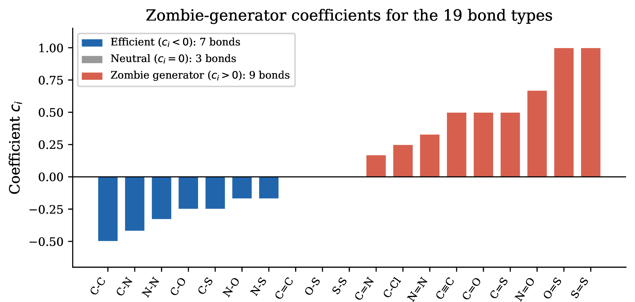
Of the \(19\) building blocks, \(9\) are zombie generators (\(c_i > 0\)), \(3\) are neutral (\(c_i = 0\)), and \(7\) are efficient (\(c_i < 0\)). The strongest zombie generators are O\({=}\)S and S\({=}\)S (\(c_i = 1\)): each double bond between low-valence atoms consumes full valence capacity.
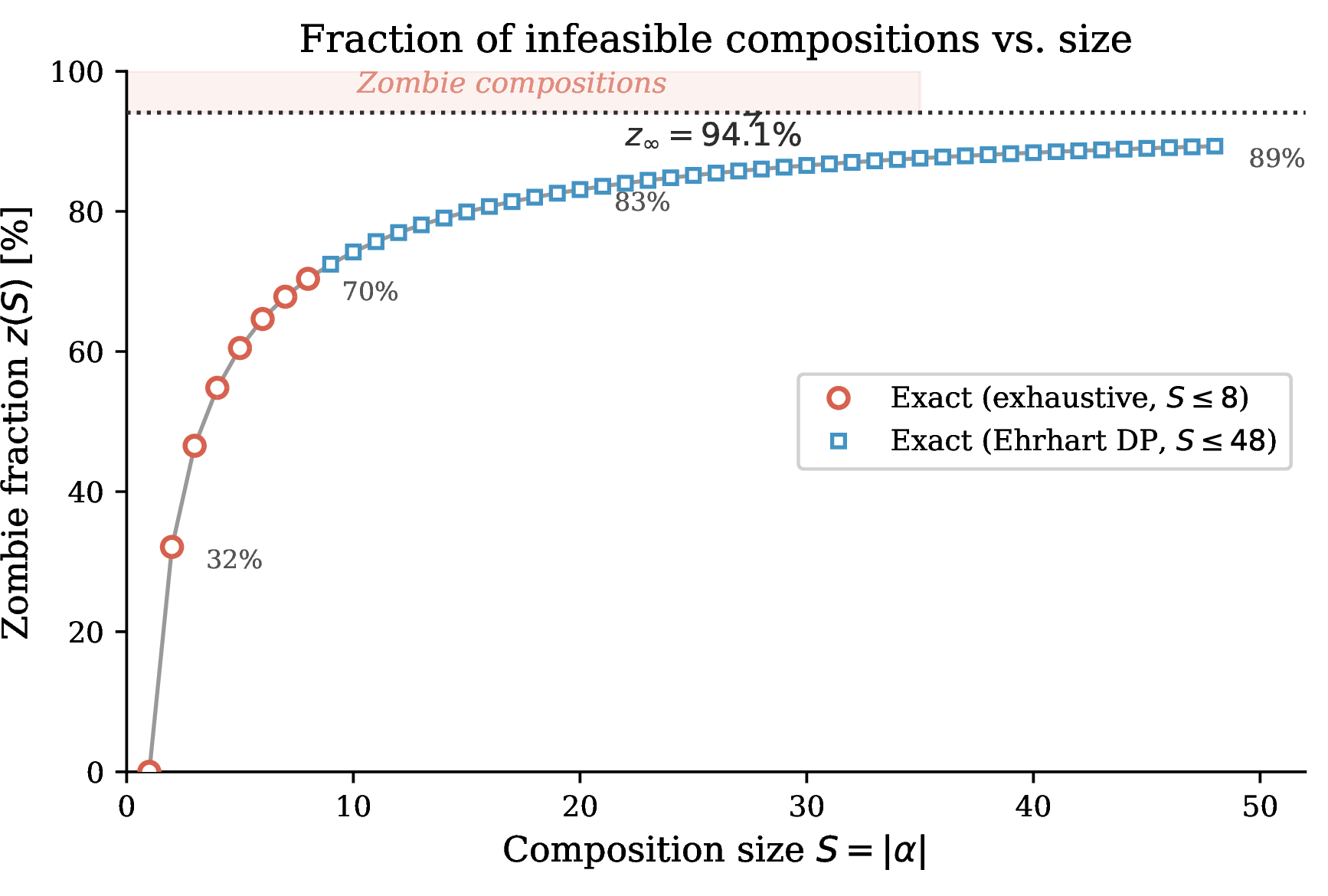
The zombie fraction is \(z(2) = 32\%\), \(z(4) = 55\%\), \(z(8) = 70\%\), and \(z_\infty = 94\%\). Already at moderate sizes, the majority of stars-and-bars compositions are chemically impossible.
The refined bound 2 has doubly-exponential exponent \(\log\log N(a) \lesssim a \cdot \log 2 \approx 0.693\,a\), strictly smaller than the fitted \(0.73\,a\) of [1].
Remark 20 (Zombie Generators and Chemical Intuition). The zombie-generator classification has a clear chemical interpretation. Single bonds between high-valence atoms (C–C: \(c = -0.50\), C–N: \(c = -0.42\)) are efficient because each atom can accommodate many bonds. Double and triple bonds between low-valence atoms (O\({=}\)S: \(c = 1.0\), S\({=}\)S: \(c = 1.0\), N\({=}\)O: \(c = 0.67\)) are zombie generators because they exhaust an atom’s bonding capacity in a single connection, requiring disproportionately many atoms for few bonds.
The asymptotic zombie fraction of \(94\%\) means that, in the limit, only \(\sim 6\%\) of the composition space is chemically realisable. Accounting for this distinction sharpens the growth exponent from \(0.73\) to \(\log 2 \approx 0.693\).
Remark 21 (Conservativity of the Bound). The valence polytope \(P_{\mathrm{val}}\) captures the aggregate constraint: the total degree demand on each atom type must be satisfiable by some number of atoms fitting within the connectivity bound. Three further sources of infeasibility are not modelled:
Pair multiplicity: a homoatomic bond of type \((t,t)\) requires \(\geq 2\) atoms of type \(t\) (no self-loops). More generally, \(k\) bonds of type \((t,t)\) need \(n_t \geq \lceil(1 + \sqrt{1+8k})/2\rceil\).
Degree-sequence realizability: the degree sequence implied by the composition must satisfy the Erdős–Gallai conditions.
Full connectivity: a graph on \(n\) vertices with \(S\) edges may be disconnected even if \(n \leq S+1\).
Each constraint can only increase the zombie fraction: \(z_\infty^{(1)} \leq z_\infty^{(1{+}2)} \leq z_\infty^{(1{+}2{+}3)} \leq \cdots\). Computationally, the pair constraint adds \(\sim\!5\) percentage points at \(S = 8\) (from \(70.4\%\) to \(75.6\%\)) but is negligible asymptotically: at \(S = 50\), both levels give \(89.5\%\) zombies (\({<}0.1\) percentage points difference).
The asymptotic negligibility of the pair constraint can be understood as follows: for typical compositions at large \(S\), the minimum atom count \(n_t \geq \lceil d_t/v_t \rceil\) already implies enough atoms of each type to satisfy the pair requirement \(n_t(n_t-1)/2 \geq k_{tt}\). The pair constraint only binds when \(n_t\) is small relative to \(k_{tt}\), which becomes increasingly rare as \(S \to \infty\).
However, the zombie fraction does not converge to \(1\) under any finite set of linear constraints. Indeed, the composition \(\alpha_S = (S, 0, \ldots, 0)\) (all C–C bonds) is feasible for all \(S\) with \(\sum c_i\alpha_i = -S/2 < 1\), so the efficient simplex face has positive volume ratio. More generally, any composition supported on efficient building blocks (those with \(c_i < 0\)) is automatically feasible. Thus \(z_\infty < 1\) for all valence-based constraints.
The bound of \(94\%\) from the valence polytope alone is therefore conservative: the true zombie fraction is at least \(94\%\) and likely higher (but strictly less than \(100\%\)).
7 Computational Results↩︎
We now present the full computational evaluation of the composition polytope for Morales Parra et al.’s molecular graph system (\(m = 19\) bond types, \(5\) atom types).
7.1 Zombie-generator coefficients↩︎
Table 1 and Figure 1 list the linear coefficient \(c_i = \sum_t D_{ti}/v_t - 1\) for each of the \(19\) bond types. Bonds with \(c_i > 0\) are zombie generators; those with \(c_i < 0\) are efficient.
| Bond type | \(c_i\) | Classification |
|---|---|---|
| C–C | \(-0.50\) | efficient |
| C–N | \(-0.42\) | efficient |
| N–N | \(-0.33\) | efficient |
| C–O | \(-0.25\) | efficient |
| C–S | \(-0.25\) | efficient |
| N–O | \(-0.17\) | efficient |
| N–S | \(-0.17\) | efficient |
| C\({=}\)C | \(\phantom{-}0.00\) | neutral |
| O–S | \(\phantom{-}0.00\) | neutral |
| S–S | \(\phantom{-}0.00\) | neutral |
| C\({=}\)N | \(+0.17\) | zombie generator |
| C–Cl | \(+0.25\) | zombie generator |
| N\({=}\)N | \(+0.33\) | zombie generator |
| C\({\equiv}\)C | \(+0.50\) | zombie generator |
| C\({=}\)O | \(+0.50\) | zombie generator |
| C\({=}\)S | \(+0.50\) | zombie generator |
| N\({=}\)O | \(+0.67\) | zombie generator |
| O\({=}\)S | \(+1.00\) | zombie generator |
| S\({=}\)S | \(+1.00\) | zombie generator |
7.2 Zombie fractions by size↩︎
Table 2 and Figure 2 compare the naïve stars-and-bars count \(\binom{S+18}{18}\) with the exact feasible count \(E_P(S) = |P_{\mathrm{val}} \cap \mathbb{Z}^{19} \cap \{|\alpha|=S\}|\), computed by exhaustive enumeration for \(S \leq 8\) and by dynamic programming on the Ehrhart quasi-polynomial for \(S \leq 48\).
| \(S\) | \(\binom{S{+}18}{18}\) | \(E_P(S)\) | Zombie % |
|---|---|---|---|
| 1 | 19 | 19 | 0.0 |
| 2 | 190 | 129 | 32.1 |
| 3 | 1 330 | 711 | 46.5 |
| 4 | 7 315 | 3 305 | 54.8 |
| 5 | 33 649 | 13 292 | 60.5 |
| 6 | 134 596 | 47 592 | 64.6 |
| 7 | 480 700 | 154 658 | 67.8 |
| 8 | 1 562 275 | 462 822 | 70.4 |
| 9 | 4 686 825 | 1 290 656 | 72.5 |
| 10 | 13 123 110 | 3 384 972 | 74.2 |
| 12 | 86 493 225 | 19 922 513 | 77.0 |
| 16 | 2 203 961 430 | 425 357 153 | 80.7 |
| 20 | 33 578 000 610 | 5 669 347 602 | 83.1 |
| \(\infty\) | — | — | 94.1 |
Values at \(S = 9, \ldots, 48\) (four full periods of the quasi-polynomial) are computed exactly by the Ehrhart DP of Proposition 17. The asymptotic value \(z_\infty = 94.1\%\) is computed via Monte Carlo estimation of \(\mathrm{Vol}(P_{\mathrm{val}} \cap \Delta_{18}) / \mathrm{Vol}(\Delta_{18}) \approx 0.059\) (\(3 \times 10^5\) Dirichlet samples).
7.3 Comparison of upper bounds↩︎
Let \(N_{\mathrm{C}}(a)\) denote the upper bound of [1] using the full stars-and-bars count, and \(N_{\mathrm{P}}(a)\) our refined bound using \(E_P(S)\) from the composition polytope. Both sum over \(S = 1, \ldots, 2^a\) with growth constant \(\gamma\).
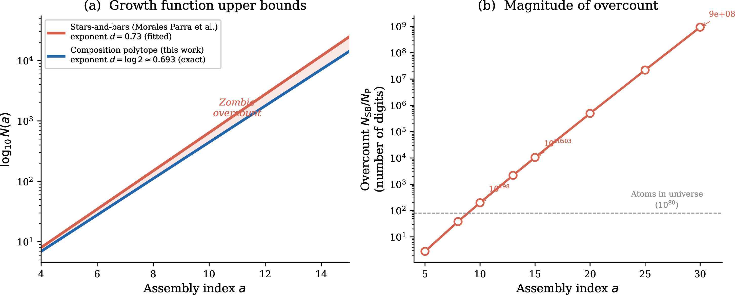
The doubly-exponential exponent—the constant \(d\) in \(\log\log N(a) \sim d \cdot a\)—determines the asymptotic behaviour. For the naïve bound, \(d_{\mathrm{C}} = 0.73\) (fitted by Morales Parra et al.). For the polytope bound, \(d_{\mathrm{P}} = \log 2 \approx 0.693\) (exact; see Corollary 1).
Table 3 and Figure 3 quantify the overcount \(N_{\mathrm{C}} / N_{\mathrm{P}}\) at selected assembly indices.
| \(a\) | \(2^a\) | \(\log_{10} N_{\mathrm{C}}\) | \(\log_{10} N_{\mathrm{P}}\) | Overcount digits |
|---|---|---|---|---|
| 5 | 32 | \(17\) | \(14\) | 3 |
| 8 | 256 | \(149\) | \(111\) | 38 |
| 10 | 1 024 | \(643\) | \(445\) | 198 |
| 13 | 8 192 | \(5\,744\) | \(3\,558\) | 2 187 |
| 15 | 32 768 | \(24\,735\) | \(14\,231\) | 10 504 |
| 20 | \(10^6\) | \(9.5 \times 10^5\) | \(4.6 \times 10^5\) | \(5.0 \times 10^5\) |
| 30 | \(10^9\) | \(1.4 \times 10^9\) | \(4.7 \times 10^8\) | \(9.4 \times 10^8\) |
At assembly index \(a = 10\), the ratio between the two bounds is \(10^{198}\). At \(a = 30\), it has \(942\) million digits. This illustrates the sensitivity of doubly-exponential bounds to the exponent: a difference of \(0.037\) in \(d\) produces enormous numerical gaps.
Remark 22 (Origin of the exponent gap). The exponent \(\log 2\) is not fitted: it is the exact base-\(e\) logarithm of \(2\) arising from \(S_{\max} = 2^a\) (Proposition 12). The difference \(\Delta d = 0.73 - \log 2 = 0.037\) between the fitted and exact exponents is consistent with the zombie fraction: including \(94\%\) additional compositions at each size \(S\) contributes \(\log(1/(1 - z_\infty)) \approx 2.81\) to the logarithm of \(N\), which accounts for \(\Delta d \approx 0.037\) when absorbed into the exponent.
8 Further Algebraic Structure↩︎
In construction systems equipped with a compatibility relation \(\perp\), one may compare the compatibility clique complex \(\mathcal{C}\) (sets whose elements are pairwise compatible) with the toric matroid \(M\). The following summarises the relationship.
Proposition 23 (Toric Containment and Characterization).
If \(\perp\) is support-separating* (compatible objects have disjoint composition supports), then \(\mathcal{C} \subseteq M\) and \(\omega(G_\perp) \leq r\).*
Equality \(\mathcal{C} = M\) holds if and only if \(M\) is a partition matroid and compatibility equals non-proportionality of compositions.
Proof. (1) Vectors with disjoint supports are linearly independent; pairwise disjoint supports imply globally disjoint supports. (2) In a partition matroid — and only in a partition matroid — pairwise independence implies global independence. The clique complex, being determined by pairs, can therefore match the matroid exactly when \(M\) has this property. Details: if \(M\) has a circuit \(\{O_1, \ldots, O_k\}\) with \(k \geq 3\), all pairs are independent (hence in \(\mathcal{C}\)), but the full set is dependent in \(M\), contradicting \(\mathcal{C} = M\). Conversely, in a partition matroid the independent sets are transversals, and non-proportionality implies membership in distinct parallel classes. ◻
Remark 24. For the click-chemistry system, \(M\) is a partition matroid with \(8\) classes, but \(76\) pairs of linearly independent compositions are incompatible (shared reactive handles), so \(\mathcal{C} \subsetneq M\) [7]. For Morales Parra et al.’s molecular graph system, all bond types are pairwise compatible and the block matroid \(M^*\) is the free matroid \(U_{19,19}\), so the containment is vacuous. The proposition is of algebraic interest but does not contribute to the growth bounds; the composition polytope (Theorem 6) is the operative tool for tightening the upper bound.
9 Discussion↩︎
The central finding of this work is that the composition polytope provides a substantially tighter upper bound on the size of molecular composition space. We now discuss the implications.
9.1 The zombie phenomenon and its origin↩︎
The observation that \(94\%\) of composition space consists of zombies is not an artefact of a particular computational method: it is a consequence of elementary valence arithmetic. Nine of the nineteen bond types in the GDB-13 system are zombie generators (\(c_i > 0\)), meaning that each such bond consumes more valence capacity per edge than the connectivity bound can sustain. When a composition is dominated by these bond types, the minimum number of atoms required to accommodate the degree demand exceeds the number of atoms available in a connected graph.
The zombie phenomenon becomes more severe with increasing composition size \(S\) because the convex body of feasible compositions (the composition polytope \(P_{\mathrm{val}}\)) occupies a shrinking fraction of the ambient simplex. The convergence to \(z_\infty = 94.1\%\) is governed by the Ehrhart–Macdonald theorem [12]: the leading term of \(E_P(S)\) scales as the volume of \(P_{\mathrm{val}} \cap \Delta_{m-1}\), which is approximately \(5.9\%\) of the full simplex volume.
9.2 Comparison with Morales Parra et al. ↩︎
Morales Parra et al.[1] derived their doubly-exponential upper bound by counting all compositions of size \(S\) via the stars-and-bars formula \(\binom{S+m-1}{m-1}\) and fitting the exponent \(d = 0.73\) from computational data. The composition polytope refines this in two ways.
First, replacing \(\binom{S+18}{18}\) by \(E_P(S)\) restricts the count to chemically realisable compositions, excluding the \(94\%\) that are zombies. Second, the exact growth exponent \(\rho = \log 2 \approx 0.693\) replaces the fitted \(0.73\), which implicitly includes the zombie contribution.
In the doubly-exponential regime these refinements are numerically significant: the ratio between the two bounds reaches \(10^{198}\) at assembly index \(a = 10\).
9.3 Exact growth exponent↩︎
The proof that \(\rho = \log 2\) (Theorem 4) resolves the gap between the lower and upper bounds. The upper bound \(\rho \leq \log 2\) follows from \(S_{\max}(a) = 2^a\) (Proposition 12). The matching lower bound is established via Pólya enumeration of trees: the composition \(\alpha_S = (S, 0, \ldots, 0)\) (all C–C bonds) is efficient (\(c_1 = -1/2\)) and its fibre contains \(T_4(S+1)\) unlabelled trees with maximum degree \(4\), growing as \(T_4(n) \sim c \cdot \gamma^n / n^{5/2}\) with \(\gamma \approx 2.48\). The centroid decomposition ensures that every such tree has assembly index \(\leq \lceil\log_2 S\rceil + 2\).
This argument shows that the exponent \(\log 2\) is intrinsic to the binary assembly model: it arises from the doubling \(S_{\max} = 2^a\) and is achieved by the simplest possible compositions. No fitted parameter is involved.
9.4 Conservativity and the hierarchy of constraints↩︎
Our zombie classification uses only the valence and connectivity constraints. Additional physical constraints—pair multiplicity, Erdős–Gallai degree-sequence conditions, and full connectivity requirements—can only increase the zombie fraction. Computationally, the pair-multiplicity constraint adds approximately \(5\) percentage points at \(S = 8\) but becomes negligible for \(S \geq 30\). This asymptotic negligibility reflects the fact that, at large sizes, the valence-derived atom counts are sufficient to satisfy pair requirements.
The strict inequality \(z_\infty < 1\) is also established: any composition supported entirely on efficient building blocks (those with \(c_i < 0\)) is automatically feasible. The seven efficient bond types (C–C, C–N, N–N, C–O, C–S, N–O, N–S) span a positive-volume face of the composition polytope, ensuring that the realisable fraction never vanishes.
9.5 Generality of the framework↩︎
The toric-geometric framework developed here is not specific to chemistry. Any construction system with a finite set of building blocks and a binary assembly operation gives rise to a toric ideal \(I_A \subset k[t_1,\ldots,t_N]\), a toric variety \(X_A\), and a matroid \(M\)—the standard objects of toric geometry [4]–[6]. The composition polytope construction applies whenever the building blocks carry a type system with bounded valence. Potential applications include combinatorial circuit design (where gates have bounded fan-in), modular construction in engineering (where connectors have limited capacity), and abstract models of biological assembly.
The click-chemistry instance (§5.2) demonstrates that the framework accommodates systems with very different combinatorial structures: a partition matroid with \(8\) classes and deterministic (unique) joining, as opposed to the free matroid and multiplicative joining of molecular graphs.
10 Conclusions↩︎
We have introduced construction systems as a general algebraic framework—rooted in the toric geometry of [4]–[6]—for studying how complex objects are built from finite sets of building blocks. The assembly process naturally gives rise to toric ideals, toric varieties, and matroids.
Applied to the molecular graph assembly system of Morales Parra et al., our framework yields three principal results.
First, the exact doubly-exponential growth exponent is \(\rho = \log 2 \approx 0.693\), proved by matching the upper bound from binary assembly trees with a lower bound from Pólya enumeration of trees. This sharpens the fitted value of \(0.73\) reported by Morales Parra et al.by excluding chemically impossible compositions from the count.
Second, the composition polytope \(P_{\mathrm{val}} \subset \mathbb{R}^{19}\) characterises all valence-feasible compositions via a single linear inequality. Its complement—the zombie region—accounts for \(94\%\) of composition space asymptotically. The zombie classification is sound (zero false positives, verified exhaustively for \(4{,}690\) compositions) and conservative: additional physical constraints can only increase the zombie fraction.
Third, the Ehrhart quasi-polynomial structure of \(E_P(S)\), with period \(12\) and degree \(18\), provides an exact counting tool for feasible compositions, refining the stars-and-bars count in every term of the growth-function sum. We have computed \(E_P(S)\) exactly for \(S = 1, \ldots, 48\) by dynamic programming on ceiling residues.
Two questions remain open. Can Pólya enumeration be restricted to the composition polytope to yield a tighter growth constant \(\gamma_P < \gamma\)? And does the partial associativity of the assembly operation endow the construction system with an operad structure whose Hilbert series recovers \(N(a)\)? These directions connect the present work to ongoing research in enumerative combinatorics and algebraic operads.