An Asynchronous Multi-Rate Taylor Method for Delay Differential Equations
June 19, 2026
Abstract
The numerical simulation of high-dimensional, multi-rate Delay Differential Equations (DDEs) is fundamentally bottlenecked by synchronous time-stepping and the dynamic memory allocation required for continuous history tracking. In this paper, we introduce the Asynchronous Adaptive Taylor Solver (AATS), an event-driven integration framework designed to overcome these high-performance computing limitations. By assigning independent local clocks to individual coordinates and advancing them using high-order Taylor polynomials generated via compile-time Automatic Differentiation, AATS restricts computational work to actively evolving sub-graphs. To eliminate the severe memory overhead endemic to traditional DDE solvers, AATS utilizes statically allocated circular buffers to store polynomial segments, achieving interpolation-free continuous dense-output evaluation with a verified zero-allocation runtime memory footprint.
Alongside this software architecture, we establish a novel continuous proof of convergence for asynchronous Taylor expansions and formally prove that the framework’s algorithmic complexity scales linearly (\(\mathcal{O}(N)\)). Extensive benchmarks against state-of-the-art synchronous solvers (Julia SciML) validate these theoretical bounds. On large-scale benchmarks (upto \(N = 10000\) coordinates) AATS fundamentally minimizes the constant factor of algorithmic work by avoiding redundant evaluations, delivering empirically consistent with \(\mathcal{O}(N)\) execution scaling and significant wall-clock speedups.
Delay differential equations, asynchronous integration, multi-rate methods, Taylor series, automatic differentiation, zero-allocation memory
65L03, 65L20, 65Y20, 65L05
1 Introduction↩︎
The numerical simulation of Delay Differential Equations (DDEs) is a cornerstone of modern computational science [1], [2], governing the modeling of systems where the rate of change depends not only on the current state but also on the system’s history. These equations naturally arise in fields characterized by inherent transmission or reaction lags, ranging from biological neural networks [3] and population dynamics [4] to control theory [5] and epidemiological modeling [6]. However, as the dimensionality of these network topologies scales to tens of thousands of coupled variables, simulating DDEs introduces profound computational bottlenecks that stretch the limits of traditional numerical integrators.
The first fundamental bottleneck is temporal. State-of-the-art numerical frameworks, like Python’s SciPy [7] or Julia’s SciML [8], almost exclusively rely on synchronous time-stepping. In a synchronous paradigm, the global integration step size \(\Delta t\) is bounded by the fastest-evolving coordinate in the network [9], [10]. For highly heterogeneous, multi-rate systems, where a few localized variables may exhibit explosive transient dynamics while the vast majority remain dormant. This shared global grid forces the solver to evaluate the entire \(N\)-dimensional system at a microscopic frequency. This leads to an overwhelming number of mathematically redundant evaluations.
The second, equally severe bottleneck is infrastructural. Unlike Ordinary Differential Equations (ODEs), which only require the current state vector to advance time, DDEs require continuous evaluation of historical states \(x(t-\tau(t))\). To achieve this, traditional solvers typically maintain two parallel data structures: a discrete integrator to advance the state, and a secondary dense-output interpolant (such as Hermite splines) to query the history continuously [1], [11]. In modern operating systems, storing and updating this history dynamically requires continuous calls to the heap manager. Over many integration steps, this dynamic memory allocation leads to catastrophic memory fragmentation, cache misses, and garbage collection latency [12], [13].
To overcome these intertwined mathematical and computational limitations, we introduce the Asynchronous Adaptive Taylor Solver (AATS). AATS is a high-performance C++ framework designed to completely abandon the shared global time grid and the reliance on dynamic memory allocation. By assigning each spatial coordinate its own independent local time domain, and by advancing these coordinates using high-order Taylor polynomials generated via compile-time Automatic Differentiation (AD) [14], AATS ensures that computational work is spent only where the local error dynamics demand it.
The primary contributions of this paper are fourfold:
Asynchronous Temporal Decoupling: We present event-driven integration, which entirely decouples the temporal evolution of multi-rate components. By employing an amortized \(\mathcal{O}(1)\) priority queue, the method bypasses the global step-size constraints imposed by rapidly changing system dynamics, ensuring that the global computational complexity scales with localized dynamics rather than worst-case properties.
Zero-Allocation History Architecture: We introduce a static memory framework for continuous history tracking. By storing fixed-degree Taylor segments within statically allocated circular buffers, the algorithm formally eliminates runtime dynamic memory allocation. This approach mathematically bounds the peak memory footprint and optimizes spatial cache locality without sacrificing historical continuity.
Interpolation-Free Delay Evaluation: We establish that the local high-order Taylor polynomials generated during integration inherently function as exact continuous state representations. By directly evaluating these polynomials, the solver evaluates continuous and state-dependent delays analytically, eliminating the computational and memory overhead associated with constructing secondary dense-output interpolants (e.g., Hermite splines).
Unified Convergence and Complexity Theory: We establish a comprehensive mathematical framework that couples the asynchronous convergence of DDE networks with their theoretical execution cost. By utilizing continuous extensions of generated Taylor polynomials, we derive strict global error bounds and delay-differential stability conditions. Furthermore, we leverage these error bounds to formally prove that the total algorithmic work scales exclusively with the localized intrinsic dynamics as a function of the user-defined tolerance \(\varepsilon\), breaking the global worst-case complexity barrier.
The remainder of this paper is organized as follows. Section 2 introduces a motivating \(10,000\)-dimensional Continuous-Time Recurrent Neural Network (CTRNN) to contextualize the multi-rate problem. Section 3 details the asynchronous algorithmic architecture and data structures. Sections 4 and 5 formalize the mathematical framework, proving the algorithmic complexity bounds and the continuous asynchronous convergence guarantees, respectively. Section 6 benchmarks AATS against the state-of-the-art Julia SciML framework, demonstrating allocation reductions and significant wall-clock speedups across varying hardware architectures. Section 7 compares AATS with current state-of-the-art. The paper concludes in Section 8.
2 A Motivating Example↩︎
To illustrate the severe computational bottlenecks inherent to traditional synchronous DDE integration, consider the simulation of a large-scale Continuous-Time Recurrent Neural Network (CTRNN) with sparse local connectivity and a uniform axonal transmission delay \(\tau=0.1\).
Let the network consist of \(N = 10,000\) neurons, where \(U(t) \in \mathbb{R}^N\) is the vector of membrane potentials. The first component \(u_1(t)\) represents a high-frequency sensory input neuron, while the remaining components \(u_2(t) \dots u_N(t)\) represent a large, slowly adapting hidden reservoir. The network dynamics are governed by the standard matrix DDE: \[\dot{U}(t) = -A \, U(t) + W \tanh(U(t-\tau)),\]
where the decay matrix \(A\) and the synaptic weight matrix \(W\) are defined as: \[A = \underbrace{\begin{bmatrix} 10^4 & 0 & \cdots & 0 \\ 0 & 1 & \cdots & 0 \\ \vdots & \vdots & \ddots & \vdots \\ 0 & 0 & \cdots & 1 \end{bmatrix}}_{\text{Rapidly changing Decay Matrix}}, \quad W = \underbrace{\begin{bmatrix} 0 & 10^4 & 0 & \cdots & 0 \\ 0.5 & 0 & 0.5 & \cdots & 0 \\ \vdots & \ddots & \ddots & \ddots & \vdots \\ 0 & \cdots & 0.5 & 0 & 0.5 \end{bmatrix}}_{\text{Sparse Tridiagonal Weight Matrix}}.\]
This architecture mathematically isolates two defining computational properties: (1) Multi-Rate changes: The spectral gap in \(A\) dictates that the sensory neuron processes inputs on a microscopic timescale (\(\approx 10^{-4}\)), while the reservoir neurons evolve on a macroscopic timescale (\(\approx 1.0\)). (2) Sparsity: To mimic biological topology, \(W\) is strictly sparse (specifically, a hollow tridiagonal structure). The local synaptic fan-in for any given neuron is explicitly bounded by \(E_v \le 2\).
2.1 The Synchronous Bottleneck↩︎
If this network is simulated using a state-of-the-art synchronous DDE solver, the step-size controller must enforce a single global integration step \(\Delta t\). To stably resolve the extreme eigenvalue of the sensory neuron, the solver is violently constrained to a global micro-step of \(\Delta t \approx 10^{-5}\).
Over a brief \(1\)-second simulation window, the synchronous solver executes \(100,000\) discrete time steps. At every single micro-step, it must evaluate the full dense vector
field for all \(10,000\) neurons. This results in \(10^9\) redundant tanh evaluations and large memory allocations to dynamically store the network’s delayed history, despite
\(99.99\%\) of the reservoir undergoing virtually no physical change.
2.2 A Proposed Coordinate-Wise Asynchronous Solution↩︎
To resolve this synchronization bottleneck, we shift to coordinate-wise asynchrony. Each variable \(u_i(t)\) is assigned an independent local clock and maintains a continuous mathematical history. Fast components evolve via independent micro-steps, while slow variables take macroscopic steps and remain dormant.
When an active variable requires delayed information (e.g., \(u_2(t-\tau)\)), it simply evaluates its neighbor’s dormant continuous trajectory algebraically, avoiding global synchronization. Exploiting network sparsity, rapid updates only trigger localized preemption checks on direct neighbors, waking them early only if their error thresholds are violated.
By decoupling temporal domains, this “sleep and wake” formulation reduces computational workload by orders of magnitude (e.g., from \(10^9\) global evaluations down to \(200,000\) localized evaluations in our example). Section 3 details the algorithmic machinery and zero-allocation memory structures enabling this scheme.
3 The Asynchronous Adaptive Taylor Solver (AATS)↩︎
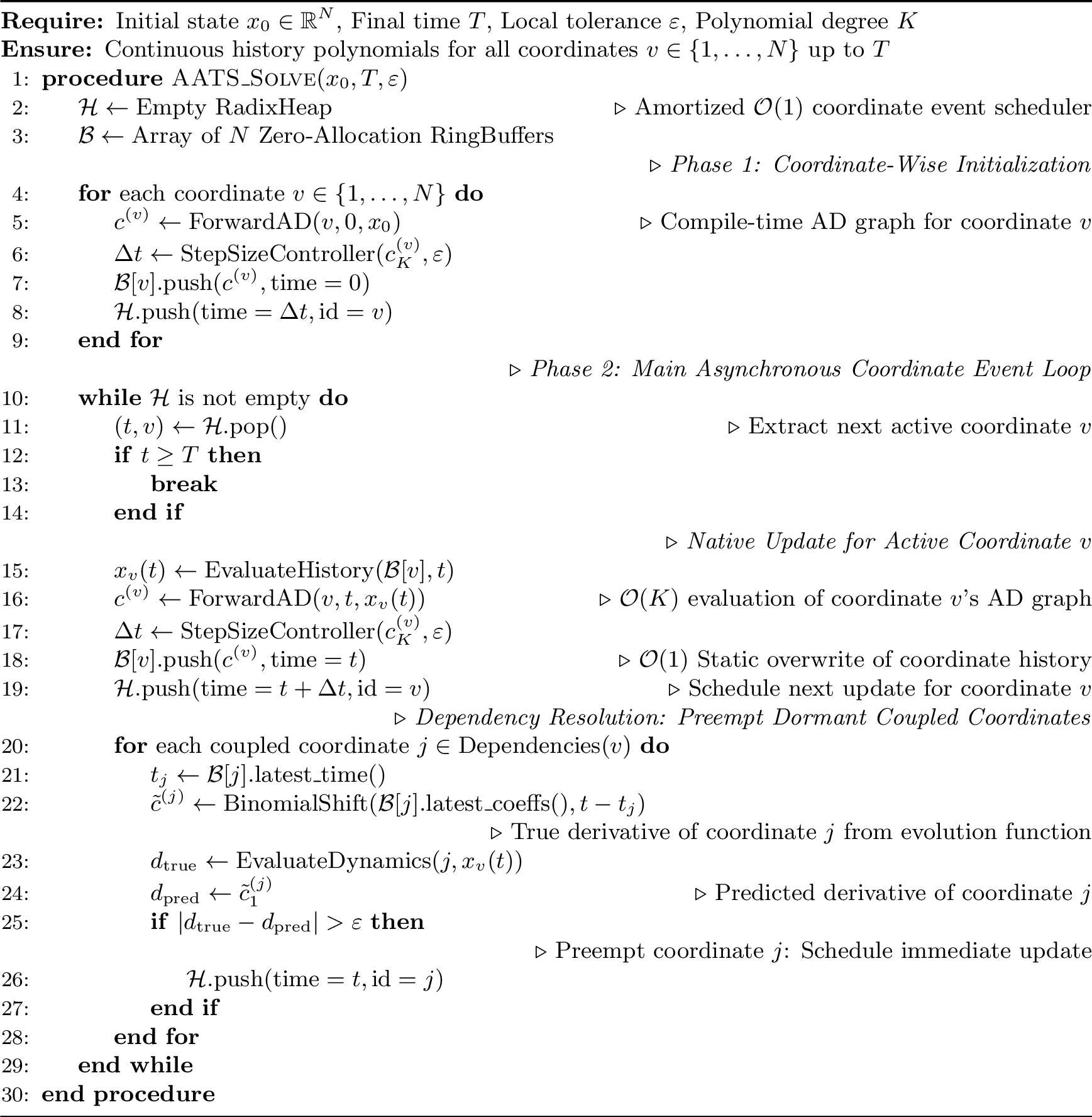
Algorithm 1 gives the pseudocode of the Asynchronous Adaptive Taylor Solver (AATS). At its core, the algorithm operates by replacing the traditional global time-step loop with an event-driven priority queue (line 2). Instead of storing discrete historical data points requiring dynamic memory allocation, AATS models the history of every coordinate2 as a continuous, piece-wise Taylor polynomial. These polynomials are statically allocated in ring buffers (line 3), strictly enforcing a zero-allocation memory footprint during runtime. The solver advances by integrating the most temporally imminent coordinate, analytically extracting delayed states from dormant neighbors, and selectively preempting those neighbors if the active coordinate’s trajectory violates their local error bounds.
3.1 Algorithmic Walkthrough of the CTRNN Simulation↩︎
We map the high-level logic of Algorithm 1 to the \(10,000\)-neuron CTRNN (Section 2), tracking an update cycle for the fast sensory neuron (\(u_1\)).
3.1.0.1 Phase 1: Initialization (Lines 4–9)
At \(t=0\), the algorithm initializes continuous trajectories (Line 5), using Automatic Differentiation (AD), and evaluates local truncation errors (Line 6). Detecting the network’s multi-rate dynamics, the controller assigns the fast neuron \(u_1\) a micro-step (\(\Delta t_1 = 10^{-5}\)) while the \(9,999\) slow reservoir neurons receive macroscopic steps (\(\Delta t_i \approx 0.1\)). Variables are queued chronologically (Lines 7–8).
3.1.0.2 Phase 2: Asynchronous Event Loop (Lines 11–19)
Assuming the simulation reaches \(t=1.0\), the scheduler pops the most imminent event: \(u_1\) (Line 11). To evaluate \(u_1\)’s nonlinear dynamics, it requires the delayed state of its neighbor, \(\tanh(u_2(t-\tau))\). Instead of forcing \(u_2\) to update, the solver directly evaluates \(u_2\)’s stored continuous history (Lines 15–16). Neuron \(u_1\) then generates its next polynomial, takes its micro-step, and reschedules (Lines 17–19).
3.1.0.3 Phase 3: Sparse Dependency Resolution and Preemption (Lines 20–28)
Because \(u_1\)’s state changed, it may invalidate the planned trajectories of its neighbors. Exploiting sparsity (Line 20), the algorithm only checks \(u_2\) (its single direct connection), safely ignoring the remaining \(9,998\) dormant neurons. It aligns \(u_2\)’s dormant trajectory to the current time (Lines 21–24) and tests the true derivative error. If the tolerance is exceeded, \(u_2\) is preempted (Lines 25–27) and forced to update immediately, guaranteeing global accuracy without synchronous barriers.
Now that we have described the working on the algorithm, we describe the high-performance techniques used to overcome the inefficiencies introduced by asynchronous integration.
3.2 Compile-Time AD Graphs↩︎
Standard runtime Automatic Differentiation (AD) incurs prohibitive tape-building overhead. AATS parses dependencies at compile time into a static, allocation-free graph. Fixing the polynomial degree \(K\) unrolls derivative expansions into Fused Multiply-Add (FMA) instructions, computing coefficients (Algorithm 1, Line 16) in pure \(\mathcal{O}(K)\) time entirely within CPU registers.
3.3 Amortized \(\mathcal{O}(1)\) Event Scheduling↩︎
To process independent coordinate updates, AATS uses a Radix Heap priority queue (Algorithm 1, Lines 11, 19). Exploiting strictly monotonic time advancement reduces event extraction to an amortized \(\mathcal{O}(1)\). Preempted dormant coordinates (Line 26) are handled via lazy deletion, allowing the queue to silently discard obsolete updates in \(\mathcal{O}(1)\) time without search-and-remove overhead.
3.4 Zero-Allocation Memory Management↩︎
Dynamic heap allocation for history tracking causes severe latency. AATS guarantees zero runtime allocations using a static array of \(N\) circular buffers, each storing \(M\) fixed-degree polynomial segments. New coefficients are pushed directly to these buffers (Algorithm 1, Line 18), natively overwriting old entries. This strictly bounds memory to \(\mathcal{O}(N \cdot M \cdot K)\) and maximizes L1 cache locality.
3.5 Binomial Time-Alignment↩︎
Evaluating coupled dynamics requires aligning dormant neighbor states at historical times (\(t_j\)) to the active time (\(t\)). Rather than triggering expensive re-evaluations, AATS projects historical states forward algebraically using a binomial expansion (Algorithm 1, Line 22). This \(\mathcal{O}(K^2)\) shift executes purely as register instructions, synchronizing dependencies without breaking the CPU pipeline.
3.6 Interpolation-Free Delay Lookup↩︎
Continuous delays typically require expensive secondary interpolants. AATS eliminates this because the integration Taylor series inherently serves as an exact dense-output representation. To evaluate a delayed state \(x(t-\tau(x(t), t))\), AATS locates the relevant buffer segment and directly evaluates the stored polynomial (Algorithm 1, Line 15), recycling AD coefficients with zero interpolation overhead.
4 Algorithmic Complexity of AATS↩︎
Traditional synchronous solvers impose an \(\mathcal{O}(N)\) or \(\mathcal{O}(N^2)\) per-step time complexity by evaluating the global state vector simultaneously, while dynamically storing continuous history requires \(\mathcal{O}(S \cdot N)\) memory over \(S\) steps. AATS circumvents these bottlenecks via asynchronous, coordinate-wise updates, with complexities formalized in the following theorems.
Theorem 1 (Local Arithmetic Time Complexity). Let \(v \in \{1, \dots, N\}\) be the active coordinate evaluated at a given asynchronous event, and let \(E_v\) denote the number of coupled neighbor coordinates (the local degree). For a Taylor polynomial of fixed degree \(K\), the amortized time complexity of a single asynchronous update in AATS is bounded by \(\mathcal{O}(E_v \cdot K^2 + K^2)\), strictly independent of the global system dimension \(N\).
Proof. The execution time of a single iteration of the main asynchronous loop (Algorithm 1, Phase 2) is the sum of four primary operations: event scheduling, state differentiation, dependency time-alignment, and continuous delay lookup.
Event Scheduling (Lines 11, 19, 26): AATS utilizes a Radix Heap for the priority queue \(\mathcal{H}\). Combined with lazy deletion for preempted events, extracting the minimum-time event (Line 11) and inserting future updates (Lines 19 and 26) both execute in amortized \(\mathcal{O}(1)\) time, independent of \(N\).
Forward Automatic Differentiation (Line 16): To generate the new polynomial segment, the solver evaluates the pre-compiled AD graph using the current coordinate state. For a coordinate with \(E_v\) coupled neighbors, aggregating the linear spatial inputs requires \(\mathcal{O}(E_v \cdot K)\) operations. Expanding the local non-linear dynamics requires \(\mathcal{O}(K^2)\) operations via discrete convolution. Calculating the full vector of Taylor coefficients \(c^{(v)}\) therefore executes in strictly \(\mathcal{O}(E_v \cdot K + K^2)\) time [14].
Dependency Time-Alignment (Line 22): For each of the \(E_v\) dormant neighbors, AATS projects their delayed state onto the active time domain \(t\) using a binomial expansion shift. Shifting a polynomial of degree \(K\) requires computing a triangular matrix-vector product, necessitating \(\frac{1}{2}K(K+1)\) operations, which is bounded by \(\mathcal{O}(K^2)\). Applying this shift across all \(E_v\) neighbors in the dependency loop yields \(\mathcal{O}(E_v \cdot K^2)\) total operations [14].
Continuous Delay Lookup (Line 15): Locating historical segment for delay \(x_j(t - \tau(t))\) in
RingBufferof maximum capacity \(M\) is \(\mathcal{O}(\log M)\) using binary search. Evaluating the \(K\)-degree polynomial at \(t_d\) requires \(\mathcal{O}(K)\) operations.
Summing these components, the total time complexity per asynchronous event is: \(\mathcal{O}(1) + \mathcal{O}(E_v \cdot K + K^2) + \mathcal{O}(E_v \cdot K^2) + \mathcal{O}(\log M + K)\)
Because the maximum polynomial degree \(K\) and the buffer capacity \(M\) are localized static constraints entirely independent of the global system dimension \(N\), the overall asymptotic time complexity per event simplifies strictly to \(\mathcal{O}(E_v \cdot K^2 + K^2)\). ◻
Theorem 2 (Global Static Memory Bound). Let \(S\) be the total number of integration steps taken to reach end time \(T\). The runtime dynamic memory allocation of AATS is strictly \(\mathcal{O}(1)\) with respect to \(S\), and the total memory footprint of the continuous history representation is permanently bounded by \(\mathcal{O}(N \cdot M \cdot K)\), where \(M\) is the fixed segment capacity of the history buffers.
Proof. During Phase 1 (Initialization) of Algorithm 1, AATS allocates an array \(\mathcal{B}\) containing exactly \(N\) zero-allocation ring buffers. Each ring buffer is initialized with a fixed capacity \(M\). A single stored segment consists of a scalar timestamp and a fixed-size array of \(K\) Taylor coefficients. Thus, the total static space required to store the continuous history for the entire state-space is exactly \(\mathcal{O}(N \cdot M \cdot K)\).
During Phase 2 (Main Asynchronous Event Loop), as \(S \to \infty\), new Taylor polynomials must be appended to the history. Because \(\mathcal{B}[v]\) utilizes modulo arithmetic to govern array indices, the \((M+1)\)-th polynomial physically overwrites the memory address of the \(1\)-st polynomial. Therefore, the amount of memory allocated during the solution trajectory is entirely independent of the number of steps \(S\) or the dynamics of the system, yielding an \(\mathcal{O}(1)\) runtime allocation footprint and guaranteeing that global memory usage never exceeds the initialized \(\mathcal{O}(N \cdot M \cdot K)\) bound. ◻
Since AATS utilizes an adaptive step size \(h\) to resolve rapidly changing or discontinuous dynamics, a quick succession of microscopic steps could theoretically exhaust the fixed history buffer. To guarantee mathematical correctness, \(M\) must be properly bounded against the system’s delay dynamics.
Lemma 1 (History Preservation Bound). Let \(M\) be the fixed capacity of the circular buffer for coordinate \(v\), and let \(h_{min}^{(v)}\) be the strict lower bound on the accepted adaptive step size. For an arbitrary state-dependent delay bounded by \(\tau_{max} = \sup \tau(t, x(t))\), continuous history preservation is strictly guaranteed if and only if: \(M \ge \left\lceil \frac{\tau_{max}}{h_{min}^{(v)}} \right\rceil + 1\)
Proof. In the worst-case scenario, coordinate \(v\) generates events of \(h_{min}^{(v)}\) time units per step. To evaluate a state-dependent delay reaching the maximum horizon \(\tau_{max}\), the buffer must retain polynomial segments spanning the interval \([t - \tau_{max}, t]\). The maximum number of segments required to span this interval under minimum step-size conditions is exactly \(\lceil \tau_{max} / h_{min}^{(v)} \rceil\). An additional slot \((+1)\) is required to safely write the active computing step without overwriting the oldest necessary boundary. ◻
Theorem 3 (Global Algorithmic Work Complexity). Let \(N_v(T)\) denote the total number of asynchronous events executed by coordinate \(v\) over the global integration interval \([0, T]\). For a system of dimension \(N\), maximum Taylor polynomial degree \(K\), and local in-degree \(E_v\), the total computational runtime \(W(T)\) of the Asynchronous Adaptive Taylor Solver is strictly bounded by: \(W(T) = \mathcal{O}\left( \sum_{v=1}^{N} N_v(T) \left(E_v K^2 + K^2\right) \right).\)
Proof. By Theorem 1, the amortized algorithmic cost of resolving a single asynchronous event for coordinate \(v\)—inclusive of event scheduling, automatic differentiation, dependency time-alignment, and history lookups—is bounded by \(\mathcal{O}(E_v K^2 + K^2)\).
Over the entire continuous integration domain \(t \in [0, T]\), the global priority queue processes exactly \(N_v(T)\) distinct events for each coordinate \(v\). Because the coordinates are strictly decoupled in time, the total algorithmic work is simply the discrete sum of the individual event costs across the entire network graph: \(W(T) = \sum_{v=1}^{N} \sum_{i=1}^{N_v(T)} \mathcal{O}\left(E_v K^2 + K^2\right).\) Factoring out the event count yields the final complexity bound. ◻
Lemma 2 (Strict Bound on Preemption Cascades). Let \(N_v^{sync}(T)\) denote the number of intrinsic, scheduled integration steps taken by coordinate \(v\) over the interval \([0, T]\) as dictated by its local error controller. The total number of preemption (or wake-up) events \(N_v^{preempt}(T)\) triggered by the structural dependencies of \(v\) is strictly bounded by: \(N_v^{preempt}(T) \le \sum_{u \in \mathcal{N}_{in}(v)} N_u^{sync}(T)\) where \(\mathcal{N}_{in}(v)\) is the set of incoming neighbors (dependencies) of \(v\).
Proof. In the AATS architecture, a preemption event for coordinate \(v\) occurs exclusively when an incoming neighbor \(u\) (Line 20–28) completes its integration step. Hence, coordinate \(v\) cannot be preempted by structurally independent variables. Therefore, the maximum number of times \(v\) can be awakened prior to its own scheduled clock expiration is exactly the sum of the intrinsic steps taken by its direct dependencies. ◻
To fully resolve the global work bound, we must express the intrinsic coordinate event counts \(N_v^{sync}(T)\) in terms of the user-defined error tolerance \(\varepsilon\). While the formal proof of adaptive error control is deferred to Section 5, we state the resulting step-count scaling here as a foundational proposition to complete our complexity profile.
Assuming the adaptive controller strictly enforces the local error bounds (as formally established in Theorem 7), the accepted maximum step sizes scale as \(h_{\max} = \mathcal{O}(\varepsilon^{1/(K+1)})\), where \(K\) is the Taylor polynomial degree. Consequently, for any coordinate \(v\), the total intrinsic scheduled event count over the finite interval \([0,T]\) is bounded by: \(N_v^{sync}(T) = \mathcal{O}(\varepsilon^{-\frac{1}{K+1}})\).
Proof. By Theorem 7, the adaptive controller guarantees
\(h_{\max} = \mathcal{O}(\varepsilon^{1/(K+1)})\). Since the total number of intrinsically accepted updates over the finite interval \([0,T]\) is strictly bounded by \(N_v^{sync}(T) \le \frac{T}{h_{\max}} + 1\), substituting the step size bound immediately yields \(N_v^{sync}(T) = \mathcal{O}(\varepsilon^{-1/(K+1)})\). ◻
Theorem 4 (Adaptive Sparsity-Dependent Linear Work Scaling). Let \(\varepsilon > 0\) be the user-defined local error tolerance. For a sparse network with bounded maximum in-degree \(E_{max} = \max_v |E_v|\) and Taylor polynomial degree \(K\), the total computational runtime \(W(T)\) of the AATS architecture scales linearly with the system dimension \(N\) and is strictly bounded by: \(W(T) = \mathcal{O}\left( N \cdot \varepsilon^{-\frac{1}{K+1}} \right)\).
Proof. By decomposing the total event count \(N_v(T)\) into intrinsic scheduled steps and preemption cascades, the total work from Theorem 3 expands to:
\[\begin{align} W(T) &= \sum_{v=1}^N \left[ N_v^{sync}(T) + N_v^{preempt}(T) \right] \mathcal{O}(E_v K^2 + K^2) \\ &\le \sum_{v=1}^N \left[ N_v^{sync}(T) + \sum_{u \in \mathcal{N}_{in}(v)} N_u^{sync}(T) \right] \mathcal{O}(E_{max} K^2 + K^2). \end{align}\]
Since each coordinate \(u\) appears in the incoming neighbor sum of at most \(E_{max}\) other coordinates, reversing the sum over the network dependencies yields (via Aggregate Analysis [15]): \(\sum_{v=1}^N \sum_{u \in \mathcal{N}_{in}(v)} N_u^{sync}(T) \le E_{max} \sum_{v=1}^N N_v^{sync}(T)\).
Substituting this algebraic bound back into the work equation gives: \[W(T) \le \mathcal{O}(E_{max} K^2 + K^2) \times (1 + E_{max}) \sum_{v=1}^N N_v^{sync}(T).\] By Proposition [prop:step95scaling], the intrinsic event count for every coordinate is uniformly bounded by \(N_v^{sync}(T) = \mathcal{O}(\varepsilon^{-1/(K+1)})\). Substituting this into the global summation yields: \(W(T) \le \mathcal{O}\left( (E_{max}^2 K^2) \sum_{v=1}^N \varepsilon^{-\frac{1}{K+1}} \right).\) Because the maximum degree \(E_{max}\) and the polynomial degree \(K\) are local constants strictly independent of the global system dimension \(N\), they factor out asymptotically. The spatial summation over the \(N\) coordinates evaluates to \(N\), yielding the final explicit bound: \(W(T) = \mathcal{O}\left( N \cdot \varepsilon^{-\frac{1}{K+1}} \right).\) ◻
This formulation highlights the core advantage of asynchronous decoupling. Synchronous solvers artificially inflate computational work by forcing slow variables to update at the frequency of the fastest component. By abandoning the shared temporal grid, AATS advances each node strictly according to its local dynamics. This guarantees optimal \(\mathcal{O}(N)\) scaling while drastically reducing the total number of algorithmic events by eliminating redundant computations.
With the computational infrastructure and hardware efficiency of AATS firmly established, the remaining imperative is to verify its mathematical integrity. The following section provides this rigorous foundation, proving that the localized step-size selection and preemption mechanics guarantee both continuous convergence and absolute stability.
5 Continuous Convergence and Stability Analysis of AATS↩︎
The fundamental departure of our analysis from traditional numerical DDE theory is its strictly continuous nature. In standard synchronous methods, stability and convergence bounds are evaluated at a shared sequence of discrete grid points \(\{t_0, t_1, \dots, t_n\}\). However, because AATS updates individual coordinates asynchronously at disjoint times, a shared global discrete grid does not exist. Consequently, traditional discrete truncation bounds are mathematically harder to apply to our algorithm. Instead, we establish stability and convergence by analyzing the globally continuous, piecewise-smooth continuous extension of the piecewise Taylor polynomials evaluated at any arbitrary time \(t \in [0,T]\), independent of the underlying event nodes.
5.1 Mathematical Setting and Assumptions↩︎
To rigorously analyze the stability and convergence of the solver, we consider a general state-dependent delay differential equation of the form: \[\dot{x}(t) = f\!\bigl( x(t), x(t-\tau(t,x(t))) \bigr), \qquad t\in[0,T],\] with an exact initial history \(x(t)=\phi(t)\) for \(t\le 0\). Here, \(f\) represents the continuous evolution function and \(\tau\) is the state-dependent delay bounded by a maximum \(\tau_{\max}\).
Let \(x_{num}(t)\) denote the continuous numerical trajectory reconstructed by AATS. Let \(h_{\max}\) denote the maximum temporal interval between any two consecutive asynchronous events generated by the scheduler. Our objective is to establish the continuous stability of \(x_{num}(t)\) and its convergence to the exact solution \(x(t)\) in the limit as \(h_{\max} \to 0\).
For the subsequent analysis, we require standard regularity conditions: we assume the evolution function \(f\), the delay \(\tau\), and the history \(\phi\) are sufficiently smooth. Furthermore, we assume \(f\) and \(\tau\) satisfy standard Lipschitz continuity bounds with respect to both the state and the delayed state. The rigid formalization of these Lipschitz constants and derivative bounds, alongside the complete mathematical proofs for the following theorems, are provided in Appendix 9.
5.2 Stability of the Continuous Asynchronous Reconstruction↩︎
In AATS, coordinates evolve independently on their own local clocks, they do not pass errors from step to step. Instead, they interact by reading each other’s continuous polynomial histories at mismatched times. Therefore, stability in AATS means that if a tiny tracking error creeps into one coordinate’s polynomial, that error must naturally fade away over time rather than magnifying across the network when its neighbors read it.
Theorem 5 (Continuous Asynchronous Stability Guarantee). Let \(e(t) := x_{num}(t) - x(t)\) define the continuous global perturbation for all \(t \ge 0\). The asynchronous reconstruction process is strictly zero-stable. The continuous propagation of errors is governed exclusively by the delay-differential inequality: \[\|e'(t)\| \le \alpha \|e(t)\| + \gamma \sup_{s \in [-\tau_{\max}, t]} \|e(s)\| + \beta(\epsilon) h_{\max}^K \quad \text{a.e.},\] where \(\alpha, \gamma > 0\) are constants characterizing the intrinsic sensitivity of the DDE (derived strictly from the system’s Lipschitz and derivative bounds detailed in Appendix 9), and \(\beta(\epsilon) > 0\) is a finite constant bounding the continuous asynchronous defect within a compact neighborhood \(\epsilon\).
Proof Sketch. Rather than measuring nodal jumps, the theorem bounds error amplification by analyzing the piecewise continuous derivative of the numerical trajectory, \(x_{num}'(t)\), defined almost everywhere. Because \(x_{num}(t)\) consists of piecewise Taylor polynomials of degree \(K\), taking its analytical derivative drops the order to \(K-1\). This generates a piecewise continuous residual (defect) function \(\rho(t)\) that is strictly bounded by \(\mathcal{O}(h_{\max}^K)\) almost everywhere. Bounding this continuous defect guarantees that overlapping asynchronous micro-steps cannot force the system into numerical instability.
5.3 Global Convergence via Continuous Integral Bounds↩︎
Having established the continuous stability of the asynchronous updates, we now demonstrate that the global trajectory converges to the true analytical solution everywhere in the domain.
Theorem 6 (Global Convergence and A Priori Stability). Under standard regularity and Lipschitz assumptions (Assumptions 1–3, Appendix 9), there exists an explicit step size threshold \(h_0 > 0\) such that for all maximum event intervals \(h_{\max} \le h_0\), the numerical trajectory strictly remains within a compact neighborhood of the true solution, and the global continuous error is uniformly bounded over the entire interval \(t \in [0, T]\) by: \[\sup_{t\in[0,T]} \|x(t) - x_{num}(t)\| = O(h_{\max}^K).\] Consequently, \(x_{num}(t) \to x(t)\) for all \(t\) as \(h_{\max} \to 0\).
Proof Sketch. Rather than assuming a priori that the numerical method is stable, the proof employs a rigorous continuous induction (bootstrap) argument. We define a compact \(\epsilon\)-tube around the exact solution. As long as the trajectory remains inside this tube, the continuous defect \(\rho(t)\) remains strictly bounded by \(O(h_{\max}^K)\). By applying a continuous Gronwall integral inequality, we constructively prove that for a sufficiently small maximum step size \(h_{\max} \le h_0(\epsilon)\), the maximum accumulated error is strictly less than \(\epsilon\), making it mathematically impossible for the trajectory to ever escape the tube before time \(T\). The full unconditional proof is detailed in Appendix 9. ◻
Theorem 7 (Adaptive Convergence Order). Assume the adaptive controller selects event intervals using a local truncation error estimator that asymptotically bounds the exact Taylor remainder. If the controller enforces a local tolerance \(\varepsilon\), then the global continuous error of the numerical trajectory satisfies: \[\|x(T) - x_{num}(T)\| = O(\varepsilon^{K/(K+1)}).\]
Proof Sketch. If the algorithmic error estimator strictly bounds the true local error from below, the local tolerance constraint \(\varepsilon\) mathematically forces the maximum accepted step size across all asynchronous coordinates to scale as \(h_{\max} = O(\varepsilon^{1/(K+1)})\). Substituting this maximum step size directly into the unconditional global convergence bound from Theorem 6 yields the \(O(\varepsilon^{K/(K+1)})\) global scaling. The formal proof, including explicit upper and lower bounding constants for the estimator, is detailed in Appendix 9. ◻
6 Numerical Validation↩︎
In this section, we empirically evaluate the Asynchronous Adaptive Taylor Solver (AATS). We benchmark our implementation against the state-of-the-art Julia SciML ecosystem (DelayDiffEq.jl). Our experiments are explicitly designed to
validate our primary theoretical contributions across five targeted metrics:
A Priori Convergence: We verify functional correctness and demonstrate that the empirical error strictly matches our derived asymptotic local truncation bounds.
Functional Equivalence: We verify that asynchronous temporal decoupling introduces zero long-term numerical drift relative to synchronous global-stepping methodologies.
Asynchronous Scalability: We evaluate algorithmic complexity, confirming the \(\mathcal{O}(N)\) event-scaling proofs as network dimensions scale to \(N=10,000\).
Sparsity-Driven Speedup: We analyze the impact of network topology, demonstrating how AATS implicitly exploits sparse dependency graphs to bypass the dense interpolation penalties of traditional solvers.
Zero-Allocation Architecture: We validate the static memory framework, proving that AATS maintains a constant, zero-byte dynamic heap utilization footprint regardless of network size.
6.1 Experimental Benchmarks↩︎
The validation suite is constructed around four distinct classes of high-dimensional delay systems. These benchmarks are specifically designed to expose the structural bottlenecks of traditional synchronous solvers—namely global dense interpolation, matrix reallocation, and the computational inefficiency of forcing a single uniform step size on systems possessing highly disparate localized timescales.
6.1.1 Benchmark 1: Concurrent Multi-Rate CTRNN↩︎
The primary benchmark models a high-dimensional Continuous-Time Recurrent Neural Network (CTRNN), serving as a large-scale computational realization of the motivating example (Section 2). The system dynamics for \(N\) neurons are governed by: \(\dot{x}_i(t) = -\alpha_i x_i(t) + \sum_{j \in \mathcal{N}_i} w_{ij} \sigma(x_j(t - \tau))\) where the constant delay is \(\tau = 0.5\), and the rational activation is defined as \(\sigma(x) = x / (1 + x^2)\). To induce extreme timescale heterogeneity, the decay rates \(\alpha_i\) are staggered: every tenth neuron is strictly fast (\(\alpha_i = 5000.0\)), while the remainder are slow (\(\alpha_i = 1.0\)).
6.1.2 Benchmark 2: Discrete Crystal Heat Diffusion (DPDE)↩︎
To evaluate performance on rapidly changing spatial gradients, we simulate a Delay Partial Differential Equation (DPDE) representing heat advection-diffusion over a discrete crystal lattice:
\(\dot{x}_i(t) = k \left( x_{i-1}(t) - 2x_i(t) + x_{i+1}(t) \right) - \gamma
x_i(t - \tau)\) where \(k=2.0\), \(\gamma=1.0\), and \(\tau=0.5\). To test the limits of local error controllers under intense spatial coupling, the
system is initialized using a smooth, continuous algebraic profile that enforces local dynamic equilibrium at \(t=0\). By avoiding discontinuous shocks, the state trajectory preserves temporal smoothness.
6.1.3 Benchmark 3: Ikeda Network DDE↩︎
The Ikeda DDE is a classic chaotic system originally formulated to model the dynamics of an optical bistable resonator [16], adapted here into a high-dimensional coupled network. It features staggered delay profiles and highly oscillatory dynamics. The system is governed by the networked equation: \(\dot{x}_i(t) = -\alpha_i x_i(t) + \sum_{j \in \mathcal{N}_i} w_{ij} \frac{x_j(t - \tau)}{1 + x_j(t - \tau)^2}\) where the delay horizon is extended to \(\tau = 1.2\). The baseline parameters alternate between variables to create deeply tangled, chaotic multi-rate trajectories. Specifically, extreme transients are induced by setting \(\alpha_i = 2500\) for every third variable (\(i \pmod 3 = 0\)), while the rest remain at a standard relaxation rate of \(\alpha_i = 1.0\). This stress-tests the asynchronous solver’s ability to maintain phase accuracy on strange attractors without global synchronization.
6.1.4 Benchmark 4: State-Dependent Mackey-Glass Network↩︎
The final benchmark stresses the solver’s continuous interpolation bounds by evaluating a highly coupled ring of State-Dependent Delay Differential Equations (SD-DDEs). This network is based on the Mackey-Glass equations [17]. In SD-DDEs, the delay horizon is a dynamic function of the local state, defined as: \(\dot{x}_i(t) = \beta \frac{x_{i+1}(t - \tau_i(x_i(t)))}{1 + x_{i+1}(t - \tau_i(x_i(t)))^4} - \gamma x_i(t)\) where \(\beta = 2.0\), \(\gamma = 1.0\), and the state-dependent delay is algebraically defined as: \(\tau_i(x_i(t)) = 1.0 + 0.5 \left( \frac{x_i(t)^2}{1 + x_i(t)^2} \right)\). This formulation forces continuous root-finding to resolve the dynamic delay horizon and fundamentally breaks the SIMD vectorization pathways of traditional synchronous solvers.
6.2 Experimental Setup↩︎
All experiments were conducted on an Apple M3 Max (14 cores, 36 GB memory). AATS was implemented in C++17 (GCC v16.0.1) with aggressive optimizations (-O3, -ffast-math, -march=native) and utilized degree \(K=4\) Taylor polynomials. The synchronous baseline was established using Julia’s SciML DelayDiffEq.jl (v1.12.6) via the
MethodOfSteps(Tsit5()) integrator. To strictly isolate algorithmic efficiency, all execution was limited to a single thread, and Julia’s absolute and relative tolerances were explicitly bound to the AATS local error tolerance \(\epsilon\).
Several alternative frameworks were excluded from the final analysis. The Python-based jitcdde solver was abandoned due to intractable memory exhaustion and compilation failures at high dimensions (\(N \ge
1000\)). We omit comparisons with RADAR5 [18], as the implicit Jacobian overhead required for stiff systems
renders algorithmic efficiency comparisons uninformative for our explicitly stable, multi-rate benchmarks. Finally, TaylorIntegration.jl [19] was excluded because it lacks native support for state-dependent delays.
6.3 Quantitative Results↩︎
6.3.0.1 A-Priori Convergence and Work-Precision Analysis
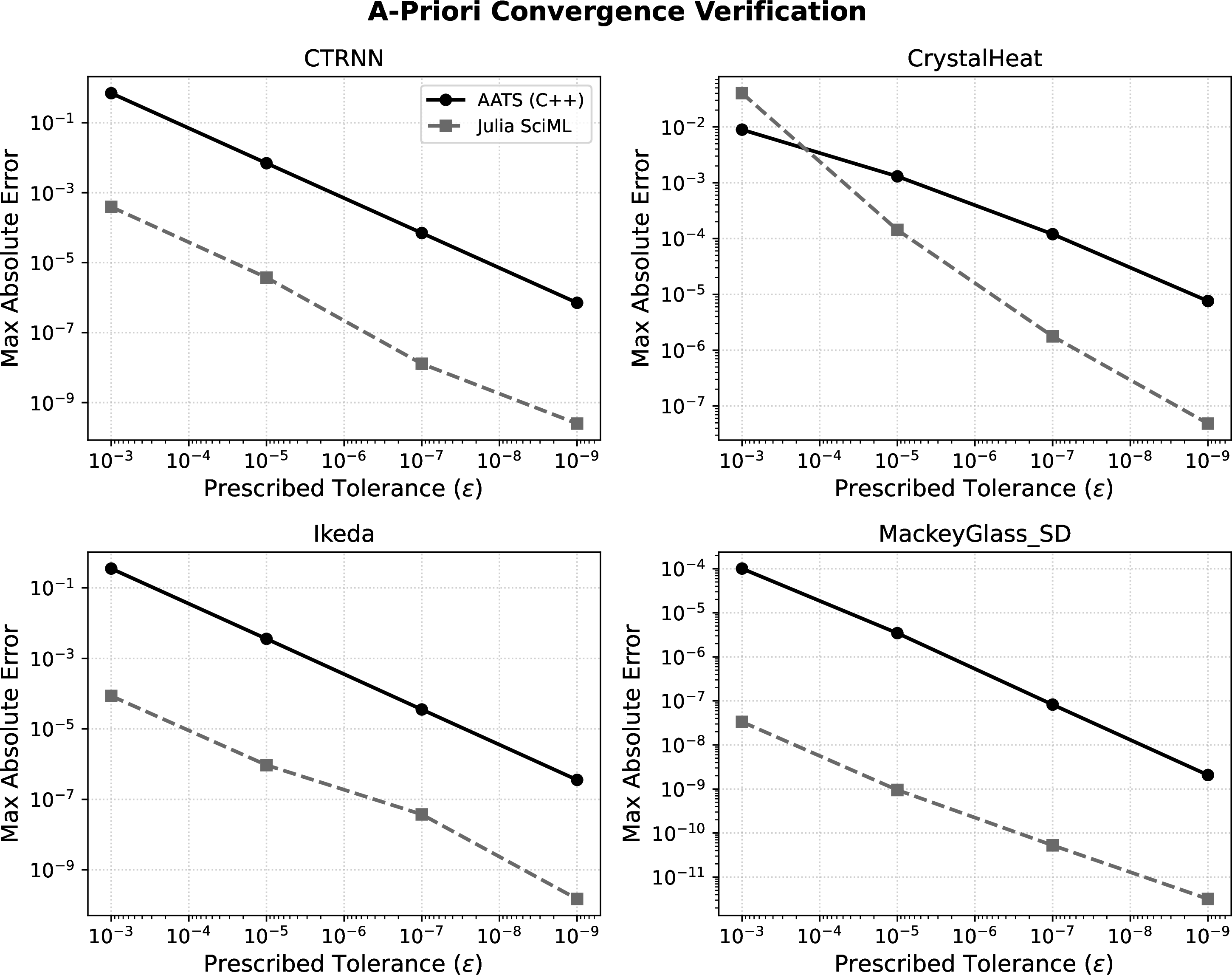
Before analyzing high dimensional scaling, we verify baseline accuracy and efficiency at \(N=10\). Figure 2 shows that AATS strictly matches the convergence slopes of the Julia SciML reference across all benchmarks, empirically validating our \(\mathcal{O}(h^{K+1})\) asynchronous truncation bounds.
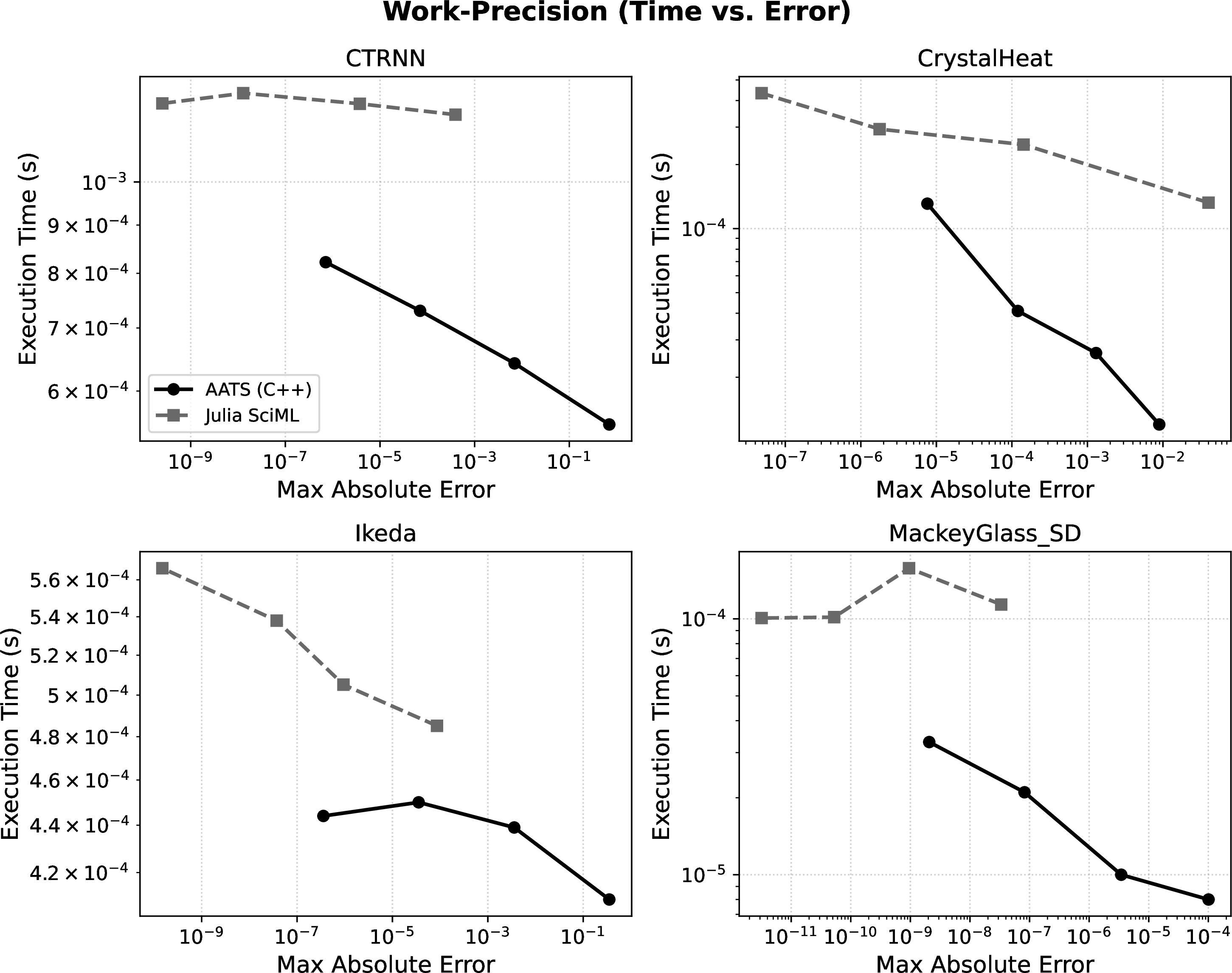
Furthermore, Figure 3 demonstrates that AATS consistently achieves lower wall-clock times for equivalent accuracy. By eliminating redundant derivative evaluations through local time-stepping, the computational savings vastly outweigh the \(\mathcal{O}(1)\) event-scheduling overhead. Even in densely coupled or highly oscillatory networks (Mackey-Glass, Ikeda), AATS comfortably outperforms the highly optimized, synchronous SciML baseline.
6.3.0.2 Functional Equivalence
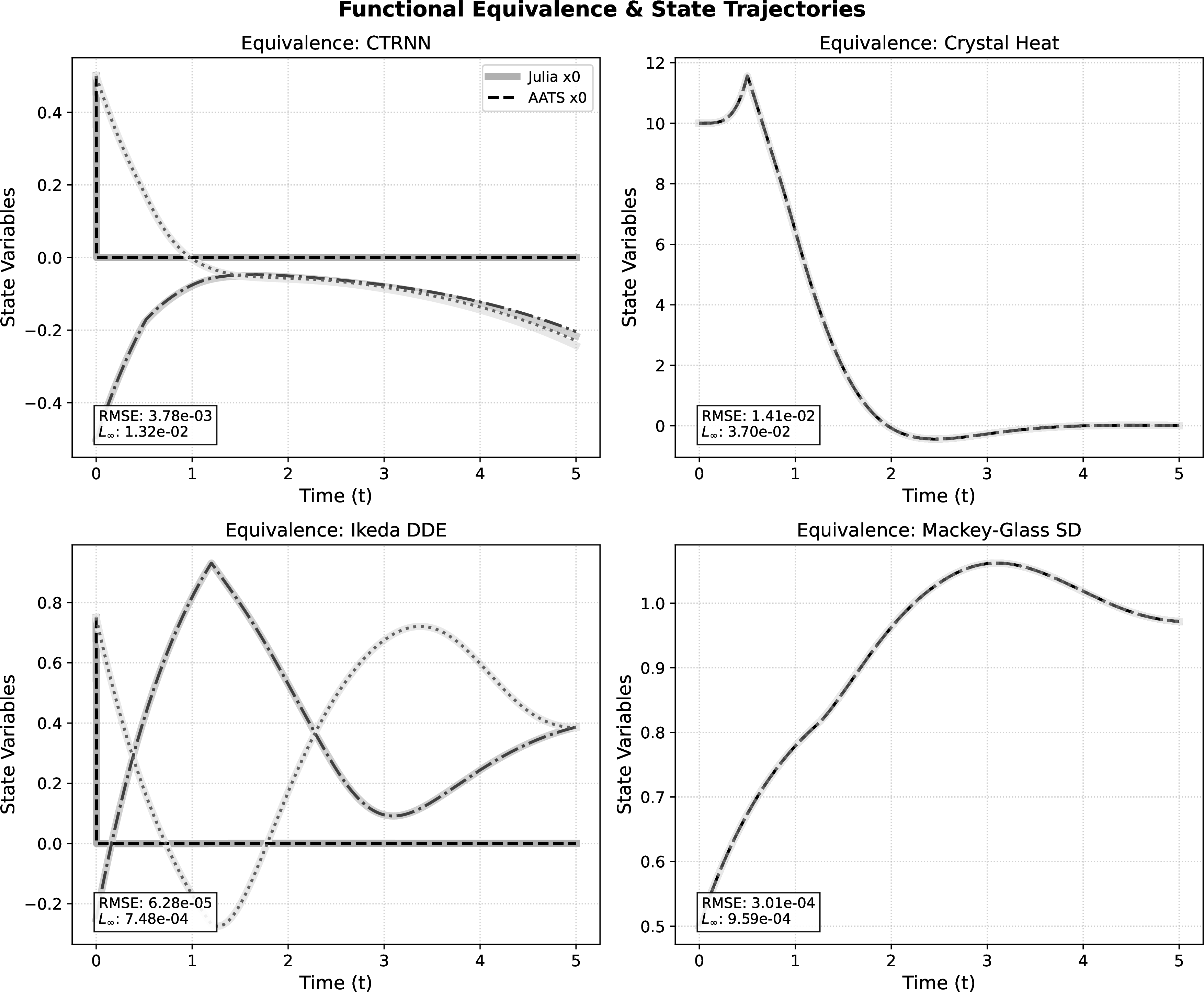
Figure 4 confirms the global functional equivalence of the AATS solver against Julia’s SciML baseline over long integration horizons. Despite nodes stepping entirely out of phase with one another, the continuous dense output of the Taylor polynomials guarantees that trajectory interactions remain precise. The low \(L_\infty\) and root-mean-square error (RMSE) metrics demonstrate that decoupling the network introduces no perceptible mathematical drift, even under chaotic (Ikeda) or state-dependent (Mackey-Glass) regimes.
6.3.0.3 Execution Speedup and Complexity
The primary computational advantage of the AATS architecture lies in its ability to bypass global synchronization bottlenecks. We quantify these performance characteristics by analyzing execution times as dimensions scale.
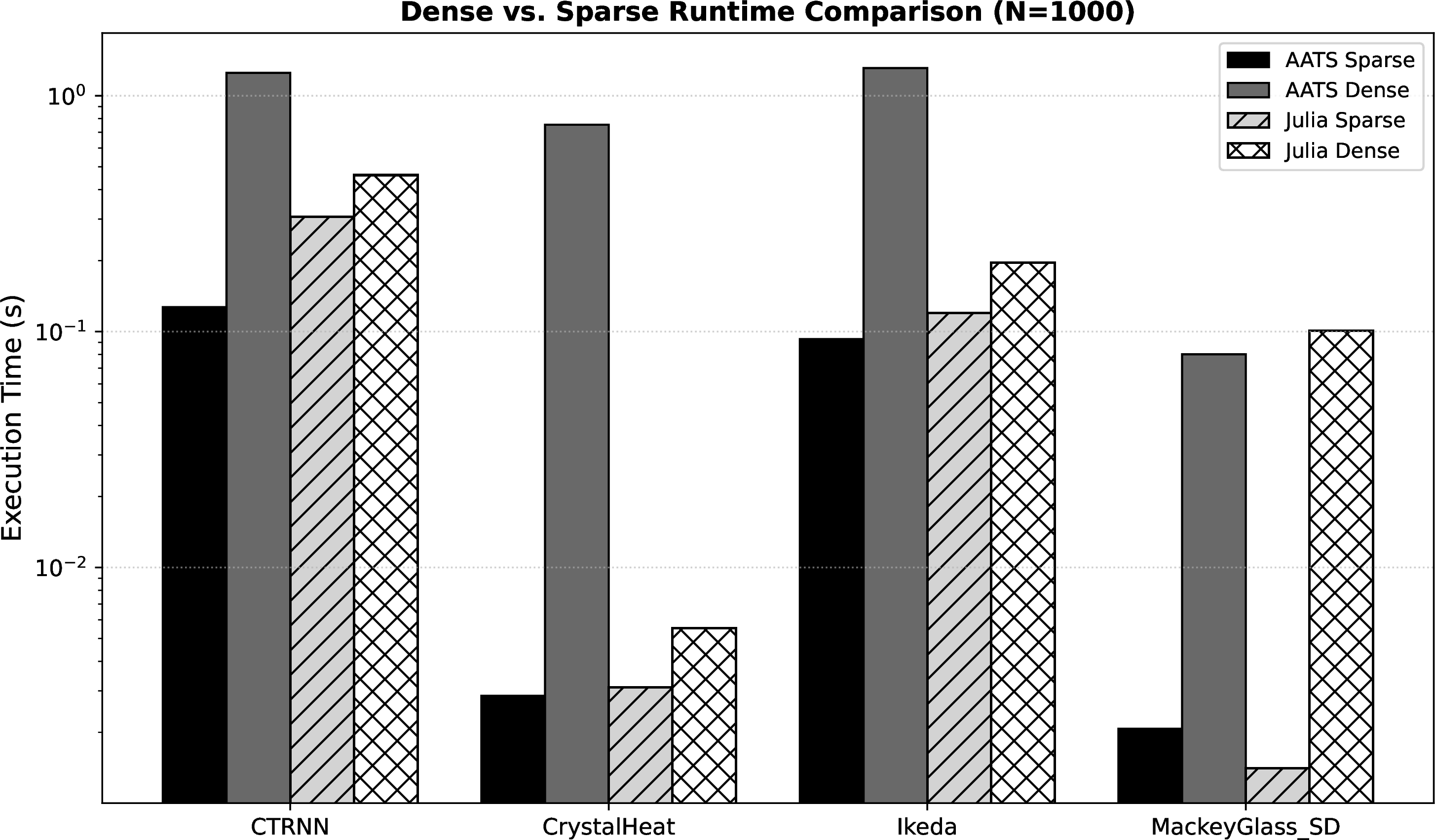
Dense vs. Sparse Topologies: AATS inherently exploits sparse networks by isolating updates to local sub-graphs, yielding order-of-magnitude speedups over SciML (Figure 5). Conversely, for fully dense systems requiring \(\mathcal{O}(N^2)\) interactions, the asynchronous event queue becomes a bottleneck. For such uniform topologies, synchronous solvers remain strictly superior by leveraging contiguous memory layouts and SIMD auto-vectorization.
Scalability of Sparse Networks: Figure 6 demonstrates empirical execution time scaling from \(N=100\) to \(N=10,000\). Because the asynchronous architecture isolates updates to local sub-graphs, it entirely bypasses the compounding global overheads and dense memory operations of traditional synchronous ecosystems. Consequently, AATS delivers strict linear time scaling that drastically outperforms the baseline’s execution speed at high dimensions.
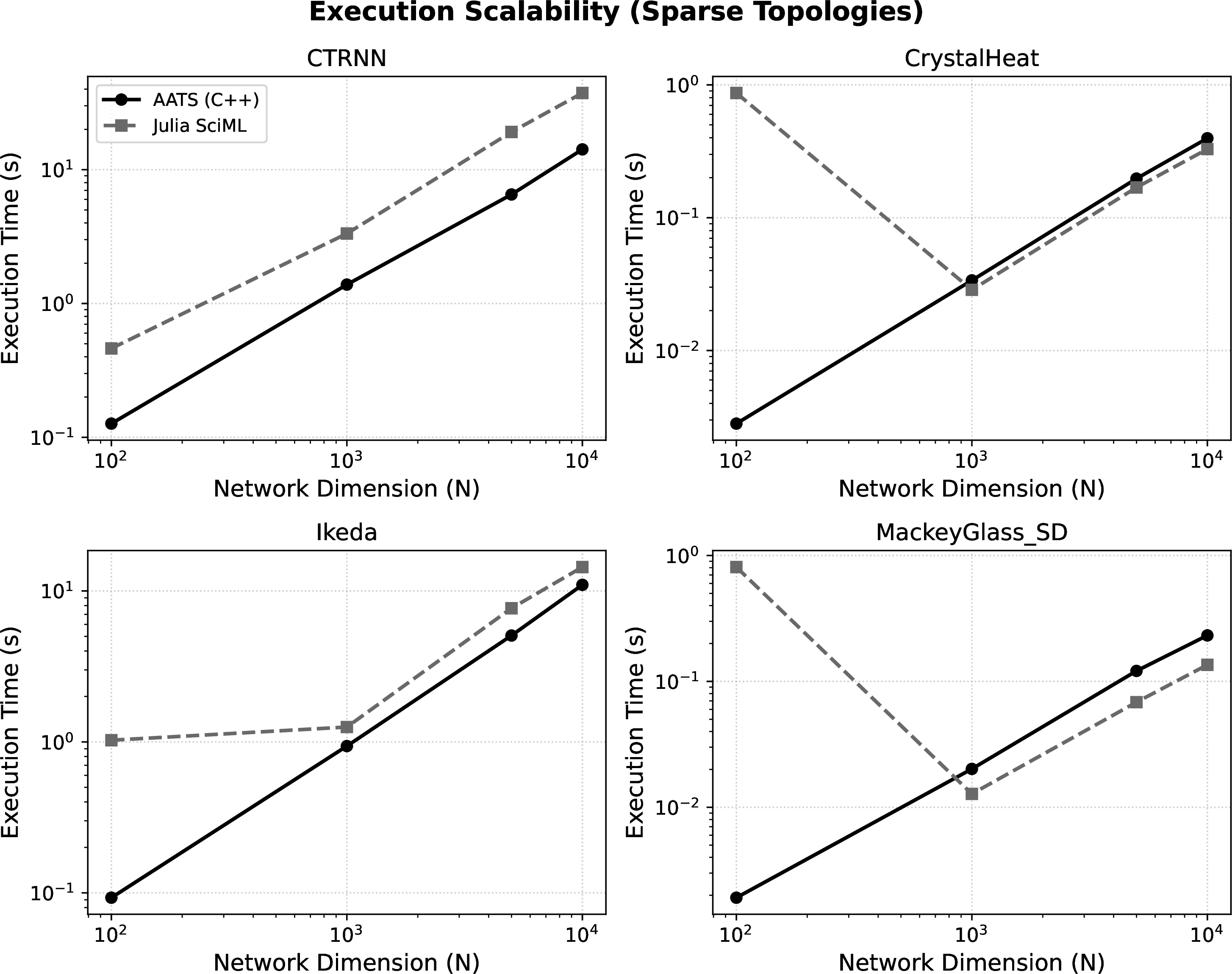
6.3.0.4 Algorithmic Complexity and Event Dynamics
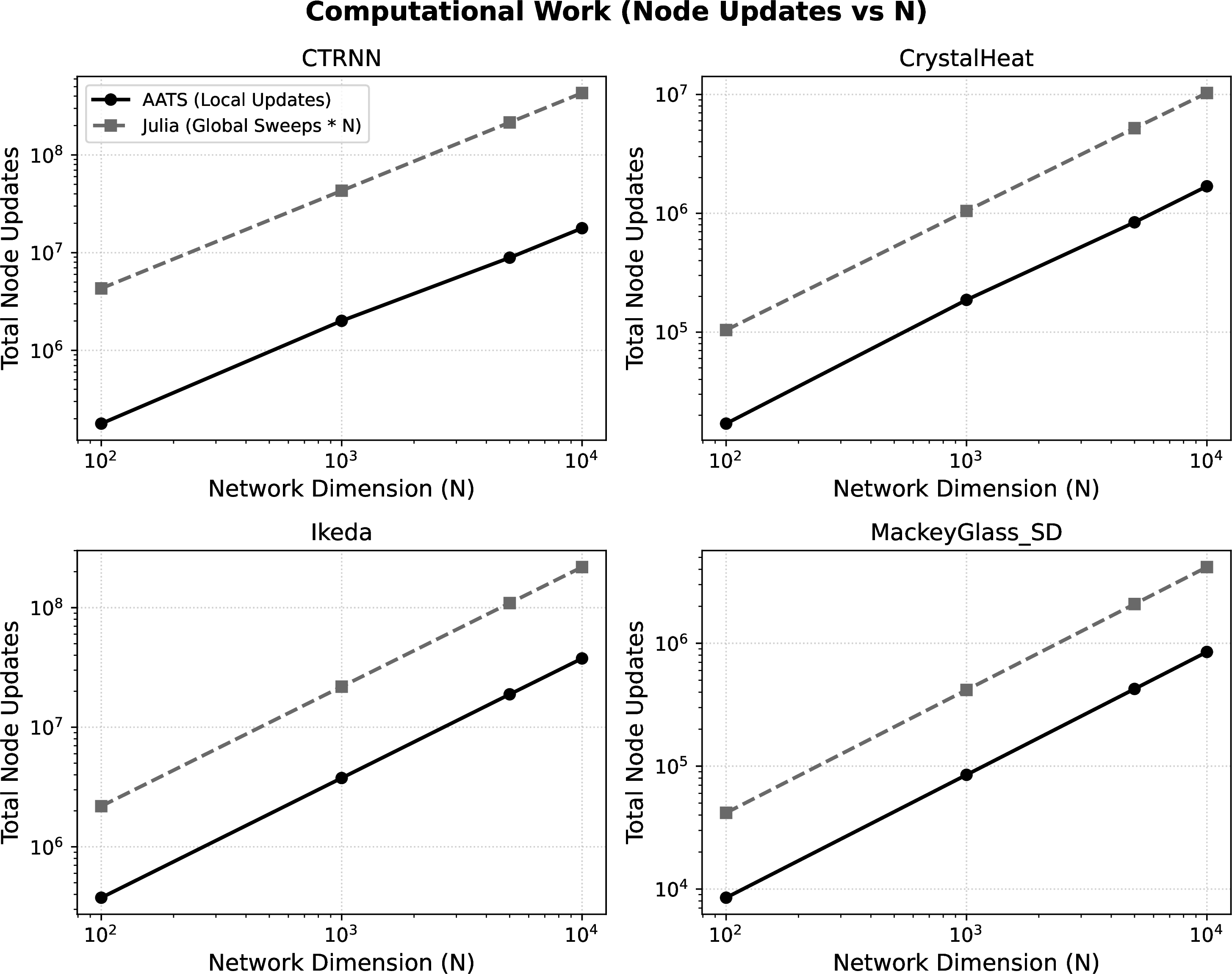
The linear execution time observed above is a direct mathematical consequence of the solver’s underlying algorithmic complexity, empirically validating Theorem 4. Figure 7 highlights the fundamental disparity in computational work (measured in total individual node updates). For sparse explicit networks, both solvers exhibit \(\mathcal{O}(N)\) linear event scaling. However, a synchronous solver (Julia) determines its global step size based on the most active variable in the network. It must step every single node forward simultaneously at this high frequency, generating a massive volume of redundant compute (an inflated constant factor). In contrast, AATS operates strictly via localized event queues. By allowing fast variables to update frequently while slow variables mathematically rest, AATS avoids millions of unnecessary evaluations. The resulting asynchronous event line runs strictly parallel to the baseline but is shifted downward.
6.3.0.5 Zero-Allocation Architecture
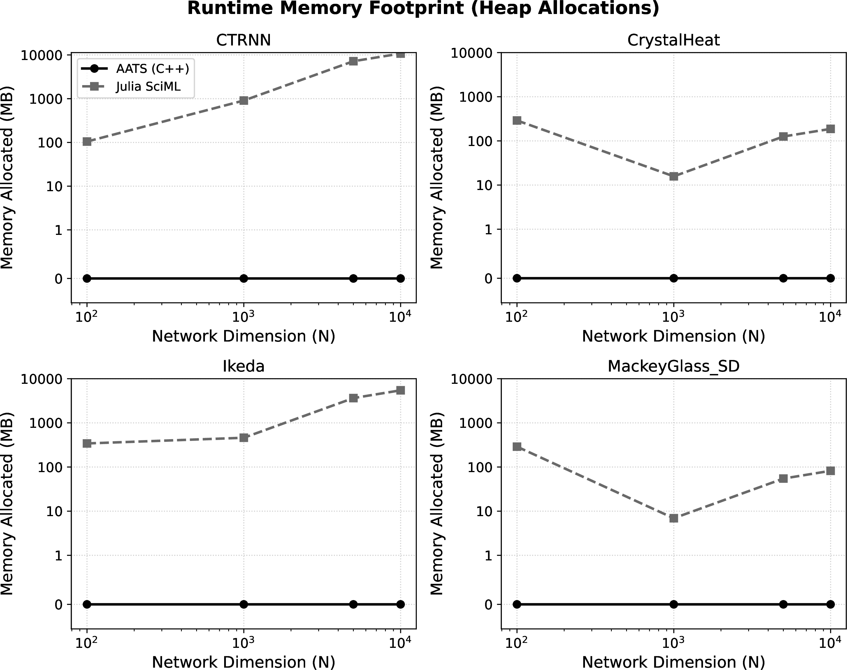
High-dimensional DDEs are memory hungry. Traditional solvers dynamically allocate large history grids and temporary interpolation arrays, relying heavily on runtime garbage collection. Figure 8 exposes this critical flaw, showing the SciML baseline’s dynamic memory footprint growing exponentially into the gigabytes as \(N\) increases.
In stark contrast, AATS relies on a static arena allocation phase during initialization. During the actual integration hot-loop, operations execute entirely on the stack and pre-allocated arrays. Consequently, the global heap tracker registers exactly \(0.0\) MB of dynamic reallocation for AATS across all dimensions. This static memory footprint eliminates garbage collection pauses, and guarantees safe execution in strictly memory-constrained environments.
7 Related Work↩︎
The Asynchronous Adaptive Taylor Solver (AATS) sits at the intersection of Taylor-series integration, multirate and asynchronous time integration, and Delay Differential Equation (DDE) simulation. While each of these areas has a rich literature, existing methods typically retain some form of global temporal structure, synchronization barrier, or secondary history reconstruction mechanism. AATS combines high-order Taylor propagation, event-driven scheduling, and continuous Taylor-history reconstruction into a unified framework that eliminates the need for a global time grid.
7.0.0.1 Taylor Series Methods and Automatic Differentiation
Modern compiler technologies and Automatic Differentiation (AD) have renewed interest in Taylor series integration. Frameworks such as TIDES [20], TaylorIntegration.jl [19], and symbolic-numeric Taylor engines [21] demonstrate that AD-generated Taylor polynomials can outperform traditional Runge–Kutta methods for many ODE problems. However, these
methods remain fundamentally synchronous: all variables advance on a common temporal grid and native support for large-scale DDEs is limited. AATS retains the arithmetic efficiency of AD-generated Taylor expansions while decentralizing polynomial
construction into independent coordinate-wise updates driven by local error control.
7.0.0.2 Multirate and Asynchronous Integration
The motivation for AATS is related to the broader multirate integration literature. Classical multirate methods, including multirate linear multistep methods [10], allow rapidly varying components to evolve with smaller time steps while slowly varying components take larger steps. More recent advances in Multirate Infinitesimal Generalized Additive Runge–Kutta (MRI-GARK) frameworks [22], [23] and decoupled multirate architectures [24], [25] extend this idea with sophisticated order conditions and flexible subsystem coupling strategies. Local Time Stepping (LTS) methods similarly reduce computational effort by assigning different time steps to different spatial regions of a system [26]. Despite their mathematical elegance and efficiency, these traditional multirate and LTS methods still retain synchronization structures through rigid macro-steps, communication stages, or strict interface boundary conditions.
7.0.0.3 Quantized State Systems
The closest conceptual relative to AATS is the Quantized State System (QSS) framework [27]. QSS methods are event-driven, component-wise, and asynchronous, making them highly effective for sparse dynamical systems. Castro et al. [28] extended QSS methods to DDEs through the reconstruction of delayed states from asynchronous trajectories. Despite these similarities, the event-generation mechanisms are fundamentally different. QSS methods generate events when state variables cross quantization thresholds. High-accuracy QSS variants (QSS2, QSS3) therefore require continuous root-finding to predict quantization crossings. As tolerances tighten, event densities may grow rapidly and quantization-induced discontinuities can complicate delayed history reconstruction. AATS instead operates entirely in the continuous-time domain. Events are generated through adaptive Taylor truncation error control rather than state quantization. Consequently, delayed histories remain continuously smooth and delay evaluations are performed without event-prediction root-finding.
7.0.0.4 Synchronous DDE Frameworks and Implicit Solvers
The dominant DDE paradigm combines a time-stepping method with a continuous history interpolant. Examples include MATLAB’s dde23 [11], Monolix [29], JiTCDDE, and the SciML ecosystem through DelayDiffEq.jl [8], [30]. These methods typically
advance all variables on a common temporal grid and reconstruct delayed states through dense-output interpolants. For stiff systems and state-dependent delays, implicit formulations such as RADAR5 [18] and SUNDIALS-based methods [31] remain among the most robust available approaches. Their strength derives from sophisticated nonlinear and linear algebra infrastructure, but this also introduces substantial global coupling costs through Jacobian
construction, factorization, and solver synchronization. In contrast, AATS replaces global synchronization with localized event-driven updates and evaluates delayed states directly from stored Taylor histories. Delayed evaluations become arithmetic
operations on existing polynomial representations rather than evaluations of secondary interpolants defined over a global time grid.
7.0.0.5 Critical Architectural Distinctions
The key distinction between AATS and existing approaches is that most multirate methods seek to reduce synchronization frequency, whereas AATS avoid global synchronization barriers. Existing methods typically retain shared temporal structures through macro-steps, Runge–Kutta stages, interface synchronization, dense-output grids, or quantization crossings. As summarized in Table 1, AATS instead combines coordinate-wise adaptive Taylor integration, event-driven scheduling, and continuous Taylor-history reconstruction within a fully asynchronous framework for DDEs.
| Method Class | Local Steps | Event-Driven | Synchronous | Native DDE |
|---|---|---|---|---|
| Classical Multirate | Yes | No | Yes | Limited |
| MRI-GARK / Multirate RK | Yes | No | Yes | Limited |
| QSS Methods | Yes | Yes | No | Partial |
| RADAR5 / DelayDiffEq / | No | No | Yes | Yes |
| JiTCDDE | ||||
| AATS | Yes | Yes | No | Yes |
4pt
7.0.0.6 The AATS Architecture
AATS synthesizes these ideas into a single high-performance architecture. High-order Taylor polynomials generated through AD provide continuous local state representations. These representations simultaneously serve as the integration mechanism, the dense-output mechanism, and the delay-history representation. As a result, arbitrary state-dependent delay evaluations can be executed as \(\mathcal{O}(1)\) polynomial evaluations within statically allocated ring buffers. The resulting framework combines continuous delay reconstruction, bounded memory usage, event-driven execution, and asynchronous multirate integration without requiring a global temporal grid.
8 Conclusion and Future Work↩︎
In this work, we introduced the Asynchronous Adaptive Taylor Solver (AATS) to overcome the severe synchronization bottlenecks of large-scale, multi-rate Delay Differential Equations (DDEs). By combining an \(\mathcal{O}(1)\) event scheduler, compile-time Automatic Differentiation, and static memory allocation, AATS strictly confines computational work to actively evolving sub-graphs while intrinsically generating continuous dense-output histories.
Crucially, we provided a novel continuous proof of convergence for asynchronous Taylor expansions and established formal \(\mathcal{O}(N)\) algorithmic complexity bounds for sparse networks. Extensive empirical validation across neural, chaotic, and spatial topologies confirms these theoretical breakthroughs. While explicit synchronous solvers can also achieve linear time scaling on sparse networks, AATS fundamentally minimizes the constant factor of computational work—allowing slow variables to mathematically rest and preventing millions of redundant evaluations—all while maintaining a verified zero-allocation dynamic memory footprint.
However, asynchronous decoupling introduces dense network overhead. Purely dense networks saturate the localized event queue. In maximally dense regimes, the queue overhead acts as a computational penalty, allowing traditional synchronous solvers to remain highly competitive by exploiting contiguous memory layouts and hardware SIMD vectorization.
Future work will focus on expanding this asynchronous framework by: (1) developing localized, SIMD-vectorized Automatic Differentiation pipelines to recover hardware efficiency in dense systems; (2) extending the AATS continuous history framework to support stiff and Stochastic Delay Differential Equations (SDDEs); and (3) parallelizing the asynchronous event queue to execute concurrent temporal updates across multi-core processors.
9 Appendix: Convergence Analysis↩︎
Consider the state-dependent delay differential equation \[\dot{x}(t) = f\!\bigl(x(t), x(t-\tau(t,x(t)))\bigr), \qquad t\in[0,T],\] with history function \[x(t)=\phi(t), \qquad t\le 0.\] Here \[x:[-\tau_{\max},T]\rightarrow\mathbb{R}^m\] denotes the exact solution, \(f\) is the governing vector field, and \(\tau\) is a state-dependent delay.
The numerical method considered in this work is an asynchronous adaptive Taylor-history solver. Each component is updated independently at event times generated by an adaptive scheduler. The solver stores local Taylor expansions and reconstructs delayed states by evaluating previously stored Taylor segments. The objective of the analysis is to establish:
consistency of the stored Taylor-history representation;
accuracy of delayed-state reconstruction;
stability of the asynchronous reconstruction process;
bounded propagation of numerical errors; and
convergence of the assembled numerical state \(x_{num}(t)\) to the exact solution \(x(t)\) as \(h_{\max}\to 0\).
The assembled numerical state produced by the solver will be denoted by \[x_{num}(t).\] The principal convergence result established is \[\sup_{t\in[0,T]} \|x(t)-x_{num}(t)\| = O(h_{\max}^{K}).\]
9.1 Event Notation↩︎
Let \[(t_k,i_k), \qquad k=0,\ldots,N-1,\] denote the sequence of asynchronous events generated by the scheduler, where \(t_k\) is the event time and \(i_k\) is the updated component. Let \(\Delta t_k\) denote the event interval generated at event \(k\), and define \[h_{\max}=\max_{0\le k<N}\Delta t_k.\] The convergence analysis is carried out in the limit \[h_{\max}\to 0.\]
9.2 Assumptions↩︎
Assumption 1 (Regularity). \(f\in C^{K+1}\), \(\tau\in C^{K+1}\), and \(\phi\) is sufficiently smooth.
Assumption 2 (Lipschitz Conditions). There exist constants \(L_0,L_d,L_\tau>0\) and a maximum delay \(\tau_{\max} < \infty\) such that \[0 \le \tau(t,x) \le \tau_{\max},\] \[\|f(x_1,y_1)-f(x_2,y_2)\| \le L_0\|x_1-x_2\|+L_d\|y_1-y_2\|,\] and \[|\tau(t,x)-\tau(t,\hat{x})| \le L_\tau\|x-\hat{x}\|.\]
Assumption 3 (Bounded Derivatives). \[M_{K+1}:=\sup_{t\in[-\tau_{\max},T]}\|x^{(K+1)}(t)\|<\infty,\] and \[M_1:=\sup_{t\in[-\tau_{\max},T]}\|x'(t)\|<\infty.\] All constants \(C,C_1,C_2,\ldots,C_T\) are independent of \(h_{\max}\).
Assumption 4 (Causality and Transversality). The state-dependent delay function \(\tau(t,x)\) satisfies the strict causality condition along the solution trajectory, meaning that the delayed time argument moves strictly forward. Formally, there exists a constant \(c_0 > 0\) such that: \[1 - \frac{d}{dt}\tau\bigl(t, x(t)\bigr) \ge c_0 > 0.\] This ensures that the historical tracking argument \(t_d(t) = t - \tau(t,x(t))\) is strictly monotonic, preventing temporal stagnation or information back-propagation.
9.3 Consistency and Reconstruction↩︎
Definition 1 (History Reconstruction Operator). Let \(R(t)\) denote the value obtained by evaluating the stored Taylor segment covering time \(t\).
Definition 2 (Assembled Numerical State). Let \(p_i(t)\) denote the most recent stored Taylor representation of component \(i\) evaluated at time \(t\). Define the global numerical state as: \[x_{num}(t) := (p_1(t), \ldots, p_m(t)).\]
Lemma 3 (Local Polynomial Consistency). Let \(p_i(t)\) be the Taylor polynomial of degree \(K\) generated by the solver for component \(i\) at an event time \(t_k\). Assuming the coefficient generation procedure is consistent of order \(K\), the local approximation error over the active interval \(t \in [t_k, t_k + \Delta t_k]\) satisfies: \[\|x_i(t) - p_i(t)\| \le C h_{\max}^{K+1},\] where \(C = \frac{M_{K+1}}{(K+1)!}\).
Proof. By the assumption of order \(K\) consistency, the generated polynomial \(p_i(t)\) matches the true local trajectory \(x_i(t)\) and its first \(K\) time derivatives evaluated at \(t_k\). Applying the standard Taylor remainder theorem to the exact scalar component trajectory \(x_i(t)\), the local truncation error is strictly bounded by the \((K+1)\)-th derivative evaluated at some intermediate point \(\xi \in (t_k, t)\).
Given Assumption 3 (Bounded Derivatives), the component error satisfies: \[\|x_i(t) - p_i(t)\| \le \frac{\|x_i^{(K+1)}(\xi)\|}{(K+1)!} (t - t_k)^{K+1}.\] Because the elapsed time \((t - t_k)\) is strictly bounded by the maximum event interval \(h_{\max}\), and the continuous state derivative is uniformly bounded by \(\|x^{(K+1)}(\xi)\| \le M_{K+1}\), the right-hand side simplifies exactly to \(C h_{\max}^{K+1}\). ◻
Lemma 4 (Local Assembled Reconstruction Error). Assuming exact state values at the most recent update events, the locally assembled numerical state over any single asynchronous interval \(t \in [t_k, t_k + \Delta t_k]\) satisfies: \[\|x(t)-x_{num}(t)\| \le C^\ast h_{\max}^{K+1}.\]
Proof. By definition, the assembled state is \(x_{num}(t)=(p_1(t),\ldots,p_m(t))\). Over a local interval where no new events occur, the true state difference is: \[x(t)-x_{num}(t) = (x_1(t)-p_1(t),\ldots,x_m(t)-p_m(t)).\] By Lemma 3, assuming exact initial conditions for the generated local polynomials, the individual components strictly satisfy \(\|x_i(t)-p_i(t)\| \le C h_{\max}^{K+1}\). Combining these componentwise bounds and applying norm equivalence in finite dimensions yields a scaled bounding constant \(C^\ast\): \[\|x(t)-x_{num}(t)\| \le C^\ast h_{\max}^{K+1}.\] ◻
Lemma 5 (Local Delayed-State Reconstruction Error). Assuming the stored Taylor segment covering the delayed time \(t_d\) was generated from exact local initial conditions, the local reconstruction error of the history operator \(R(t_d)\) satisfies: \[\|x(t_d) - R(t_d)\| \le \frac{M_{K+1}}{(K+1)!} h_{\max}^{K+1},\] where \(M_{K+1} = \sup_{t} \|x^{(K+1)}(t)\|\) over the local integration domain.
Proof. Because the history reconstruction operator \(R(t)\) evaluates a previously finalized polynomial segment exactly as defined in Lemma 3, this bound evaluates the localized Taylor remainder formula at the historical time point \(t_d\). Like the assembled dense state, this strictly bounds the local truncation error of the history representation prior to the accumulation of global error. ◻
Remark 1 (Continuity Across History Segments). Adjacent Taylor segments are generated sequentially from continuous state values enforced at event times, guaranteeing that the global history reconstruction operator \(R(t)\) remains \(C^0\)-continuous across all segment boundaries. Consequently, when a dynamic or state-dependent delay forces the historical argument \(t_d\) to cross a segment boundary, the operator smoothly transitions between independent polynomial pieces. Because each piece satisfies Lemma 5 natively, the reconstruction error remains bounded uniformly by \(\mathcal{O}(h_{\max}^{K+1})\), avoiding the localized interpolation mismatches or artificial order reduction characteristic of static grid-allocation schemes.
9.4 Delay Perturbation Analysis↩︎
Define the error \[e(t):=x_{num}(t)-x(t).\] Let \[t_d=t-\tau(t,x(t)), \qquad \hat{t}_d=t-\tau(t,x_{num}(t)).\]
Lemma 6. \[|t_d-\hat{t}_d| \le L_\tau\|e(t)\|.\]
Proof. By definition, \[|t_d-\hat{t}_d| = |\tau(t,x_{num}(t))-\tau(t,x(t))|.\] Applying the Lipschitz condition on \(\tau\) gives \[|t_d-\hat{t}_d| \le L_\tau\|x_{num}(t)-x(t)\| = L_\tau\|e(t)\|.\] ◻
Lemma 7. If \(\|x'(t)\|\le M_1\), then \[\|x(t_d)-x(\hat{t}_d)\| \le M_1L_\tau\|e(t)\|.\]
Proof. By the mean-value theorem, \[\|x(t_d)-x(\hat{t}_d)\| \le M_1|t_d-\hat{t}_d|.\] Applying the previous lemma yields \[\|x(t_d)-x(\hat{t}_d)\| \le M_1L_\tau\|e(t)\|.\] ◻
9.5 Error Propagation and Continuous Defect↩︎
Define the global error \(e(t):=x_{num}(t)-x(t)\).
Definition 3 (Piecewise Continuous Defect). Let \(\hat{t}_d=t-\tau(t,x_{num}(t))\). Because the assembled numerical state \(x_{num}(t)\) is constructed from piecewise Taylor segments, it is globally continuous (\(C^0\)) but its derivative \(x_{num}'(t)\) possesses jump discontinuities at the event times \(t_k\). Therefore, we define the continuous residual, or defect, almost everywhere (for \(t \neq t_k\)) as: \[\rho(t) := x_{num}'(t) - f(x_{num}(t), x_{num}(\hat{t}_d)).\] This function measures how exactly the analytical derivative of the assembled numerical polynomial satisfies the governing dynamics evaluated at the reconstructed numerical state on the open intervals between events.
Definition 4 (Compact \(\epsilon\)-Tube). Let \(\epsilon > 0\). The compact \(\epsilon\)-neighborhood around the exact continuous solution history is defined as: \[\Omega_\epsilon := \left\{ y \in \mathbb{R}^m : \min_{t \in [-\tau_{\max}, T]} \|y - x(t)\| \le \epsilon \right\}.\]
Lemma 8 (Piecewise Bounded Evolution Derivatives). Under Assumption 1, \(f, \tau \in C^{K+1}\). Because the assembled numerical state \(x_{num}(t)\) is constructed from piecewise polynomials of degree \(K\), it is globally \(C^0\) and its time derivatives up to order \(K\) are piecewise continuous.
Crucially, the delayed argument \(t_d(t) = t - \tau(t, x_{num}(t))\) maps current integration times back into the numerical history, potentially crossing the discrete boundaries where history segments transition. Under Assumption 4 (Causality), the delayed argument is strictly increasing (\(1 - \frac{d\tau}{dt} > 0\)), forcing \(t_d(t)\) to pass transversally through these segment transitions. Because the set of asynchronous event times is finite over the bounded interval \([0,T]\), the pre-image of these discrete boundaries under the strictly monotonic mapping \(t_d(t)\) is also finite. Consequently, the set of times where the numerical trajectory evaluates exactly on a non-smooth historical boundary has Lebesgue measure zero.
Therefore, the multivariate chain rule expansion of the \(K\)-th time derivative \(F^{(K)}(t)\) exists and is piecewise continuous almost everywhere (specifically, avoiding local event updates and their delay-induced echoes).
Let \(\Omega_\epsilon\) be the compact \(\epsilon\)-neighborhood defined in Definition 4. Because \(F^{(K)}(t)\) is a piecewise continuous mapping composed of \(C^{K+1}\) functions evaluated over a bounded domain, its magnitude is bounded almost everywhere. We can thus explicitly define the finite constant \(M_F(\epsilon) < \infty\) as the essential supremum of this derivative mapping: \[M_F(\epsilon) := \operatorname*{ess\,sup} \left\{ \|F^{(K)}(t)\| : x_{num}(s) \in \Omega_\epsilon \text{ for all } s \le t \right\}.\]
Consequently, for any arbitrary bootstrap interval \([0, t^*] \subseteq [0,T]\) where the numerical trajectory satisfies \(x_{num}(s) \in \Omega_\epsilon\) for all \(s \le t^*\), the continuous evolution function
\(F(t) = f(x_{num}(t), x_{num}(t-\tau(t,x_{num}(t))))\) strictly satisfies: \[\|F^{(K)}(t)\| \le M_F(\epsilon) < \infty \quad \text{a.e.}\]
Lemma 9 (Component-Wise Exactness of Algorithmic Coefficient Generation). Let \(t_k^{(i)}\) be the event time at which component \(i\) is asynchronously updated. Because the solver maintains dense-output polynomials \(p_j(t)\) for all components \(j = 1, \dots, m\), the numerical state \(x_{num}(t)\) is a fully defined, piecewise-polynomial vector function.
Provided the delayed argument \(t_d = t_k^{(i)} - \tau(t_k^{(i)}, x_{num}(t_k^{(i)}))\) lies in the interior of a stored history segment, the delay composition is differentiable through order \(K\). Because historical segment boundaries form a set of measure zero, this condition holds almost everywhere.
Under this condition, when the Taylor arithmetic and forward-mode Automatic Differentiation pipeline executes for component \(i\) at \(t_k^{(i)}\), the generated coefficients for the local polynomial \(p_i(t)\) exactly match the Taylor coefficients of the \(i\)-th component of the numerical composite function: \[F_i(t) = f_i(x_{num}(t), x_{num}(t-\tau(t,x_{num}(t))))\] evaluated strictly at \(t = t_k^{(i)}\), up to the truncation order \(K\) used by the method.
Proof. This relies fundamentally on the architecture of asynchronous dense-output. The AD pipeline does not merely read the scalar values of neighboring components \(j \neq i\); it reads their \(K\)-th degree polynomial representations \(p_j(t)\). As long as the delayed evaluation avoids exact segment boundaries (which occurs a.e.), the historical argument accesses a purely smooth \(C^\infty\) polynomial function.
Because the standard rules of algorithmic Taylor arithmetic exactly preserve univariate and multivariate series composition [14], [19], [32], the AD engine evaluates the exact temporal derivatives of \(F_i(t)\) at the specific local event time \(t_k^{(i)}\). The extension to state-dependent delay systems preserves this exactness because retrieving historical state components maps strictly to evaluating an explicit history polynomial \(P_{\text{hist}}\) via standard algebraic Cauchy multiplication. ◻
Lemma 10 (Assembled Global Truncation Defect). Assuming the exact algorithmic generation of local Taylor coefficients up to degree \(K\), the assembled global continuous defect \(\rho(t) := x_{num}'(t) - F(t)\) satisfies the strict bound: \[\|\rho(t)\| \le \frac{M_F(\epsilon)}{K!} h_{\max}^K,\] almost everywhere for any \(t \in [0, T]\), provided the numerical trajectory remains strictly within the compact tube \(\Omega_\epsilon\).
Proof. We construct the global defect bound by analyzing the system component-wise. At any given continuous time \(t \in (0, T)\) not exactly on an event boundary, every component \(i \in \{1, \dots, m\}\) is governed by its most recently generated polynomial \(p_i(t)\), updated at some local event time \(t_k^{(i)} \le t\).
The local continuous defect for component \(i\) is defined as \(\rho_i(t) := p_i'(t) - F_i(t)\). Because \(p_i(t)\) is a polynomial of degree \(K\), its derivative \(p_i'(t)\) is a polynomial of degree \(K-1\). By Lemma 9, \(p_i'(t)\) exactly matches the Taylor expansion of \(F_i(t)\) around \(t_k^{(i)}\) up to degree \(K-1\).
Applying the standard Taylor remainder theorem for a \((K-1)\)-degree polynomial strictly to the \(i\)-th component yields: \[|\rho_i(t)| \le \frac{\sup_{\xi} \|F_i^{(K)}(\xi)\|}{K!} (t-t_k^{(i)})^K.\]
By definition of the asynchronous scheduler, the elapsed time since the local update is strictly bounded by the maximum global event interval: \((t-t_k^{(i)}) \le \Delta t_k^{(i)} \le h_{\max}\). Furthermore, because the assembled numerical trajectory \(x_{num}(s)\) is confined to the compact tube \(\Omega_\epsilon\), Lemma 8 guarantees that the continuous \(K\)-th derivative of the vector field is uniformly bounded almost everywhere by \(M_F(\epsilon)\).
Consequently, every individual component strictly satisfies: \[|\rho_i(t)| \le \frac{M_F(\epsilon)}{K!} h_{\max}^K \quad \text{a.e.}\]
Because this strict \(\mathcal{O}(h_{\max}^K)\) upper bound holds simultaneously for all components \(i=1, \dots, m\) on their respective active asynchronous intervals, it assembles directly into the global vector defect norm: \[\|\rho(t)\| = \|x_{num}'(t) - F(t)\| \le \frac{M_F(\epsilon)}{K!} h_{\max}^K \quad \text{a.e.}\] ◻
From the definition of the continuous defect and the true analytical derivative \(x'(t) = f(x(t), x(t_d))\), the continuous error dynamics exactly satisfy almost everywhere (for \(t \neq t_k\)): \[e'(t) = x_{num}'(t) - x'(t) = f(x_{num}(t),x_{num}(\hat{t}_d)) - f(x(t),x(t_d)) + \rho(t).\]
To simplify notation in the subsequent error bounds, we explicitly define the local truncation defect constant parameterized by the tube radius \(\epsilon\): \[\beta(\epsilon) := \frac{M_F(\epsilon)}{K!}.\]
Using the Lipschitz property of \(f\) and substituting the bound on the continuous defect, we can bound the piecewise derivative of the error: \[\|e'(t)\| \le L_0\|e(t)\| + L_d\|x_{num}(\hat{t}_d)-x(t_d)\| + \beta(\epsilon) h_{\max}^K \quad \text{a.e.}\]
To handle the delayed state difference, we add and subtract the true state evaluated at the approximate delayed time, \(x(\hat{t}_d)\), and apply the triangle inequality: \[\|x_{num}(\hat{t}_d)-x(t_d)\| \le \|x_{num}(\hat{t}_d)-x(\hat{t}_d)\| + \|x(\hat{t}_d)-x(t_d)\|.\]
The first term on the right-hand side is exactly the global error evaluated at the approximate delayed time, \(\|e(\hat{t}_d)\|\). Since \(\hat{t}_d \le t\), we can bound this by the supremum of the error over the history up to time \(t\). Let \(\|e_t\| := \sup_{s \in [-\tau_{\max}, t]} \|e(s)\|\). Then, \[\|x_{num}(\hat{t}_d)-x(\hat{t}_d)\| = \|e(\hat{t}_d)\| \le \|e_t\|.\]
Applying the delay perturbation lemma to the second term yields
\(\|x(\hat{t}_d)-x(t_d)\| \le M_1L_\tau\|e(t)\|\). Substituting these bounds back into the delayed state difference gives: \[\|x_{num}(\hat{t}_d)-x(t_d)\| \le \|e_t\| +
M_1L_\tau\|e(t)\|.\]
Substituting this into the differential inequality for \(\|e'(t)\|\) and grouping the non-delayed terms yields: \[\|e'(t)\| \le (L_0 + L_d M_1 L_\tau)\|e(t)\| + L_d \|e_t\| + \beta(\epsilon) h_{\max}^K \quad \text{a.e.}\]
Letting \(\alpha = L_0 + L_d M_1 L_\tau\), we obtain the fundamental piecewise delay-differential inequality governing the error propagation: \[\|e'(t)\| \le \alpha\|e(t)\| + L_d \|e_t\| + \beta(\epsilon) h_{\max}^K \quad \text{a.e.}\]
9.6 Bounded Continuous Error Propagation↩︎
To establish a global bound on the error, we employ a delay-differential extension of Gronwall’s inequality. Because the defect bounding constant \(M_F(\epsilon)\) requires the trajectory to remain inside the compact tube \(\Omega_\epsilon\), the error propagation must first be established conditionally.
Lemma 11 (Conditional Bounded Error Propagation). Assume the numerical trajectory remains strictly inside the compact neighborhood \(\Omega_\epsilon\) over an arbitrary bootstrap interval \([0, t^*] \subseteq [0,T]\). Then there exists a finite constant \(C_T(\epsilon) > 0\) such that the error satisfies: \[\sup_{t\in[0,t^*]}\|e(t)\| \le C_T(\epsilon) h_{\max}^{K}.\]
Proof. Since \(\|e(t)\| \le \|e_t\|\), we can simplify the differential bound to: \[\|e'(t)\| \le (\alpha + L_d)\|e_t\| + \beta(\epsilon) h_{\max}^K \quad \text{a.e.}\]
Because \(e(t)\) is absolutely continuous (globally \(C^0\) and piecewise \(C^1\)), its fundamental theorem of calculus holds over the integration domain. Integrating from \(0\) to \(t\) (for \(t \le t^*\)) and applying the triangle inequality yields: \[\|e(t)\| \le \|e(0)\| + \int_0^t \left( (\alpha + L_d)\|e_s\| + \beta(\epsilon) h_{\max}^K \right) ds.\]
Because the right-hand side is a monotonically non-decreasing function of \(t\), it strictly bounds the supremum of the left-hand side over the interval \([0, t]\). Assuming exact initial history conditions (i.e., \(\|e(0)\| = 0\)), we obtain an integral inequality for the supremum function: \[\|e_t\| \le \beta(\epsilon) t h_{\max}^K + \int_0^t (\alpha + L_d)\|e_s\| ds.\]
Applying the standard continuous Gronwall’s lemma [33] to the scalar function \(u(t) = \|e_t\|\) yields: \[\|e_t\| \le \beta(\epsilon) t h_{\max}^K \exp\left((\alpha + L_d)t\right).\]
Evaluating this bound up to the maximal domain time \(T\) yields an unconditionally safe upper bound for any \(t^* \le T\): \[\sup_{t\in[0,t^*]}\|e(t)\| \le \left[ \beta(\epsilon) T \exp\left((\alpha + L_d)T\right) \right] h_{\max}^K.\]
Defining the constant \(C_T(\epsilon) := \beta(\epsilon) T \exp\left((\alpha + L_d)T\right)\) completes the proof. ◻
9.7 Global Convergence↩︎
Theorem 8 (Global Convergence and A Priori Stability). Under Assumptions 1, 2, and 3, there exists an explicit step size threshold \(h_0 > 0\) such that for all maximum event intervals \(h_{\max} \le h_0\), the global numerical error satisfies: \[\sup_{t\in[0,T]} \|x(t)-x_{num}(t)\| \le C_T(\epsilon) h_{\max}^{K}.\]
Proof. We establish this using a bootstrap argument (continuous induction). Choose an arbitrary tube radius \(\epsilon > 0\) and let \(\Omega_\epsilon\) be its corresponding compact neighborhood.
We explicitly select the step size threshold \(h_0(\epsilon)\) such that the maximum theoretically accumulated error bounded by Lemma 11 remains strictly less than the chosen tube radius \(\epsilon\): \[h_0(\epsilon) := \left( \frac{\epsilon}{2 C_T(\epsilon)} \right)^{1/K}.\]
Assume for the sake of contradiction that the numerical trajectory escapes the tube \(\Omega_\epsilon\) before the final time \(T\). Let \([0, t^*]\) be the maximal bootstrap interval, where the escape time \(t^*\) is defined as: \[t^* := \sup \{ t \in [0,T] : \|x(s) - x_{num}(s)\| \le \epsilon \text{ for all } s \in [0, t] \}.\]
Because the solver is initialized with exact history conditions (\(\|e(0)\| = 0 < \epsilon\)) and the numerical trajectory is piecewise continuous, \(t^* > 0\).
For the entire bootstrap interval \([0, t^*)\), the numerical trajectory remains strictly in the interior of \(\Omega_\epsilon\). Thus, by topological compactness, Lemma 8 ensures \(M_F(\epsilon)\) remains finite, which strictly validates the delay-differential Gronwall error propagation in Lemma 11. By continuity, exactly at the escape time \(t^*\), the error must satisfy \(\|e(t^*)\| = \epsilon\).
However, because the solver operates with a maximum step size \(h_{\max} \le h_0(\epsilon)\), applying the conditional Gronwall bound over the validated bootstrap interval \([0, t^*]\) guarantees: \[\|e(t^*)\| \le C_T(\epsilon) h_{\max}^K \le C_T(\epsilon) h_0(\epsilon)^K = \frac{\epsilon}{2} < \epsilon.\]
This is a strict mathematical contradiction. The continuous error cannot simultaneously equal \(\epsilon\) and be bounded by \(\epsilon/2\). Therefore, our assumption of escape is false, and \(t^* = T\).
Consequently, the numerical trajectory never escapes the compact tube \(\Omega_\epsilon\) during the integration domain \([0,T]\). This closes the bootstrap loop, satisfying the condition for Lemma 11 globally, yielding the final convergence bound: \[\sup_{t\in[0,T]} \|x(t)-x_{num}(t)\| \le C_T(\epsilon) h_{\max}^K.\] ◻
Corollary 1 (Uniform Convergence). \[\sup_{t\in[0,T]} \|x(t)-x_{num}(t)\| = O(h_{\max}^{K}).\]
9.8 Adaptive Error Control↩︎
Unlike embedded Runge-Kutta methods that rely on carefully tuned coefficient tableaus to estimate local error, Taylor-series methods natively possess an intrinsic error estimator. By evaluating the magnitude of the highest-order computed term (or the difference between a \(K\)-th and \((K-1)\)-th degree expansion), the solver directly measures the local truncation error. Provided the \((K+1)\)-th derivative of the state trajectory does not entirely vanish, this algorithmic estimator strictly mirrors the theoretical asymptotic scaling. We formalize this as an operational assumption for the adaptive controller:
Assumption 5 (Asymptotically Exact Error Estimator). The asynchronous adaptive controller evaluates event intervals using a local truncation error estimator \(\eta(h)\) that perfectly captures the theoretical polynomial scaling. There exist positive constants \(c_1, c_2 > 0\) such that for any sufficiently small event interval \(h\): \[c_1 h^{K+1} \le \eta(h) \le c_2 h^{K+1}.\]
Theorem 9 (Adaptive Convergence Order). Under Assumption 5, if the controller strictly enforces the local tolerance bound \(\eta(h) \le \varepsilon\) across all asynchronous components, then the global numerical error satisfies: \[\|x(T) - x_{num}(T)\| = O(\varepsilon^{K/(K+1)}).\]
Proof. By Assumption 5, any accepted step size \(h\) must satisfy the local tolerance constraint \(\eta(h) \le \varepsilon\).
Applying the lower bound of the estimator’s asymptotic behavior, we have: \[c_1 h^{K+1} \le \eta(h) \le \varepsilon.\]
Rearranging this inequality to isolate the step size \(h\) yields: \[h \le \left( \frac{\varepsilon}{c_1} \right)^{\frac{1}{K+1}}.\]
Because this bound applies universally to all accepted steps across all asynchronous coordinates, the maximum global event interval \(h_{\max}\) is strictly bounded by: \[h_{\max} = O(\varepsilon^{1/(K+1)}).\]
From the Unconditional Global Convergence theorem, we have already rigorously established that the global error is bounded by \(C_T(\epsilon) h_{\max}^K\). Substituting our bound for \(h_{\max}\) into this global error bound yields: \[\|x(T) - x_{num}(T)\| \le C_T(\epsilon) \left( \left( \frac{\varepsilon}{c_1} \right)^{\frac{1}{K+1}} \right)^K = \frac{C_T(\epsilon)}{c_1^{K/(K+1)}} \varepsilon^{K/(K+1)}.\]
Because \(C_T(\epsilon)\) and \(c_1\) are constants independent of \(\varepsilon\), it immediately follows that the global error scales strictly as \(O(\varepsilon^{K/(K+1)})\). ◻
References↩︎
Department of Electrical, Computer, and Software Engineering, University of Auckland, NZ (avinash.malik@auckland.ac.nz)↩︎
In the context of network or multi-dimensional differential equations, each node, vertex, or individual state variable maps directly to a distinct spatial coordinate in the system’s state space \(\mathbb{R}^N\).↩︎