1 Introduction↩︎

In Maxwell electrodynamics the geometrical-optics limit has a simple meaning: the wave vector of light is null with respect to the spacetime metric. In that case, the optical cone and the gravitational null cone are the same, and photon propagation can be studied directly from the background geometry [1], [2]. This picture changes in nonlinear electrodynamics (NLED). The Born–Infeld theory and the Heisenberg–Euler effective action already showed that the electromagnetic response can depend on the field itself [3]–[9]. The electromagnetic field then behaves as a medium, and the physical light cone is fixed not only by the metric, but also by the constitutive law of the theory.

This is the natural language of the covariant formulation of NLED. In Plebański’s approach one works with the field \(F_{\mu\nu}\), the excitation \(P_{\mu\nu}\) and the electromagnetic invariants. The mixed formulation of Salazar, García and Plebański is especially useful when the relation between field and excitation is more basic than a single elementary Lagrangian written globally as \(L(\mathcal{F},\mathcal{G})\) [10]–[12]. In this view, the optical problem is not added to the geometry from outside. It is part of the same electromagnetic response. The works of Boillat, Novello et al., and Obukhov and Rubilar showed that the characteristic equation of a nonlinear electromagnetic theory can become a Fresnel quartic and, in many cases, can split into two quadratic cones [13]–[17]. This splitting is the geometrical origin of vacuum birefringence in NLED.

When NLED is coupled to gravity, the electromagnetic field has two roles. It sources the spacetime through the Einstein equations, and it also determines the optical cone followed by high-frequency electromagnetic perturbations [18]–[25]. Therefore, for an Einstein–NLED black hole, null geodesics of the background metric are not always the physical photon trajectories. One has to use the effective optical geometry selected by the constitutive response. This point has become important in studies of regular black holes, effective metrics, light rings, shadows and perturbations [26]–[31]. In particular, the recent study of axial electromagnetic quasinormal modes in a static Plebański-type NLED black hole shows that the same nonlinear sector can also leave dynamical imprints [31]. The present paper is complementary to that direction: here we focus on the geometrical-optics and critical-curve side.

Black hole shadows are a natural place to see this difference. Since the works of Bardeen and Luminet, the edge of the shadow has been related to unstable photon orbits and to their projection on the observer screen [32], [33]. This idea was later developed for analytical shadow constructions, finite-distance observers, deformed compact objects and non-Kerr geometries [34]–[46]. The observational relevance of the subject increased after the Event Horizon Telescope images of M87* and Sagittarius A* [47]–[59]. Also, the study of photon rings and higher-order lensing bands has made clear that small changes in the critical structure can be important in ideal images [60]–[67].

The present work sits at this intersection: effective optical geometry in NLED and critical curves of rotating black holes. For static and spherical solutions, the optical problem can often be reduced to an effective light-ring radius. For a rotating spacetime the problem is richer. The shadow is controlled by critical families, impact parameters, angular motion and a local tetrad projection. In Kerr and Kerr–Newman geometries, this structure is tractable because the Hamilton–Jacobi equation separates, as shown by Carter [68]–[72]. This separability is related to hidden symmetries, Killing tensors and principal tensor structures [73]–[76]. It is then natural to ask what remains of this structure when the photon does not follow the spacetime metric itself, but an optical metric produced by NLED. We keep contact with standard treatments of spherical photon motion, Kerr lensing bands and nonequatorial critical structures [77]–[80].

The exact rotating García–Díaz solution provides a useful laboratory for this question. It is an exact stationary and axially symmetric solution of Einstein gravity coupled to NLED, with mass, rotation, electric and magnetic charges, and electrodynamic parameters controlling the nonlinear branch [81], [82]. Its Maxwell limit is the dyonic Kerr–Newman solution [83], [84]. For nonzero nonlinear coupling, both the metric function and the electromagnetic potentials are modified. Ayón–Beato showed that the electrodynamics behind this solution is naturally recovered in the mixed formulation, even when the supporting Lagrangian cannot be written globally in elementary form [85]. Thus, the optical problem should not be treated as a phenomenological deformation added by hand. It has to be obtained from the constitutive response of the exact solution. This also connects the present work with studies of rotating regular black holes and nonlinear electromagnetic sources [86]–[88]. We also keep contact with Newman–Janis-type constructions and related rotating NLED models [89]–[94].

In this paper we follow the optical chain step by step. First, we write the García–Díaz metric and its two mixed potentials in a principal tetrad. This gives an aligned form for the field and excitation, described by four scalars \(E\), \(B\), \(D\) and \(H\). Second, we use these scalars to reconstruct the local constitutive branch connected with the Maxwell limit, written as \((D,B)\mapsto(E,H)\). Third, we compute the response matrix and insert it in the Fresnel construction. Finally, we study the Hamilton–Jacobi problem, build the branch-dependent critical families and project them on the screen of a finite-distance observer.

The main message is simple. The nonlinear electromagnetic structure does not only modify the background metric. It also changes the characteristic cones that control high-frequency electromagnetic propagation. For the rotating García–Díaz branch studied here, the Fresnel quartic splits into two optical roots. At the perturbative order used in this work, both roots admit a Carter-type separation. Each optical branch therefore has its own radial and angular potentials, its own critical constants and its own projected critical contour. The birefringent signal appears as a doubling of the critical structure: the two curves collapse to one curve in the Maxwell limit, but separate when the nonlinear response is active.

The paper is organized as follows. In Sec. 2 we present the García–Díaz metric, the mixed potentials, the principal tetrad and the aligned electromagnetic scalars. In Sec. 3 we reconstruct the local constitutive branch and obtain its response matrix. In Sec. 4 we derive the Fresnel cones and the optical metrics. In Sec. 5 we discuss the Hamilton–Jacobi equations and show that both optical branches admit a Carter-type separation at the order considered. In Sec. 6 we construct the two branch-dependent critical families, project them on a finite-distance observer screen and introduce geometrical diagnostics of the splitting. In Sec. 7 we discuss the physical meaning, scope and observational relevance of the result. We close in Sec. 8. Numerical details, parameter scans and reproducibility information are collected in Appendix 9.

2 García–Díaz background and aligned fields↩︎

We first fix the exact background that will be used in the rest of the paper. This includes the metric, the mixed electromagnetic potentials, the principal tetrad and the simple algebraic identities followed by the aligned field. The purpose of this section is only to prepare the geometrical and electromagnetic data. The constitutive interpretation will be made in the next section, where the relation between field and excitation is read directly from these exact quantities.

We work in units \(G=c=1\), with signature \[(-,+,+,+), \label{eq:signature95convention}\tag{1}\] and in an exterior region where the principal tetrad used below is regular.

2.1 Metric, parameters, and asymptotic structure↩︎

We adopt as background the rotating García–Díaz solution in Boyer–Lindquist-type coordinates [81], [85], \[\begin{align} ds^2={}& \Sigma\,d\theta^2 +\frac{\sin^2\theta}{\Sigma} \Bigl[a\,dt-(r^2+a^2)d\phi\Bigr]^2 +\frac{\Sigma}{\Delta}\,dr^2 \\ &-\frac{\Delta}{\Sigma} \Bigl(dt-a\sin^2\theta\,d\phi\Bigr)^2 \end{align} \label{eq:GDmetric}\tag{2}\] where \[\begin{align} \Sigma&=r^2+a^2\cos^2\theta,\\ \Delta&=r^2+a^2-2Mr +(p^2+q^2)\Bigl[1-\beta(r^2+a^2)\Bigr]^2 . \end{align} \label{eq:SigDelta}\tag{3}\] Here \(M\) is the mass, \(a\) is the rotation parameter, and \(q\) and \(p\) are the electric and magnetic charges of the branch under consideration. Since this is an Einstein–NLED solution, these charges should not be viewed merely as a formal copy of the Maxwell sector, but as part of the exact constitutive branch that supports both the electromagnetic field and the geometry [81], [85].

In the original presentation of the family, in addition to \(\beta\), further electrodynamic constants usually denoted by \(F_0\) and \(G_0\) appear and encode part of the invariant structure of the underlying theory [81], [82]. In this work these constants are kept fixed, and we restrict the analysis to the sector \[(M,a,p,q,\beta). \label{eq:parameter95sector}\tag{4}\] The parameter \(\beta\) controls the nonlinear deformation that appears both in the electromagnetic potentials and in the radial function \(\Delta\). Since the combination \(\beta(r^2+a^2)\) is dimensionless, \[[\beta]=L^{-2}, \qquad \ell_\beta\sim |\beta|^{-1/2}, \label{eq:beta95dimension95scale}\tag{5}\] so that \(\ell_\beta\) sets the radial scale associated with the nonlinearity.

Two limits provide immediate checks on the solution. In the linear limit, \[\Delta\big|_{\beta=0} = r^2+a^2-2Mr+(p^2+q^2), \label{eq:Delta95Maxwell95limit}\tag{6}\] the geometry reduces to the dyonic Kerr–Newman sector [81], [83]. On the other hand, when the rotation is switched off one obtains \[ds^2\big|_{a=0} = -f(r)\,dt^2+\frac{dr^2}{f(r)} +r^2(d\theta^2+\sin^2\theta\,d\phi^2), \label{eq:static95metric95limit}\tag{7}\] with \[f(r)= 1-\frac{2M}{r} + \frac{p^2+q^2}{r^2}\bigl(1-\beta r^2\bigr)^2. \label{eq:static95lapse95limit}\tag{8}\] The same family therefore contains both the linear dyonic limit and a nonlinear static sector.

The asymptotic structure requires an additional precaution. From 3 , as \(r\to\infty\), \[\begin{align} \Delta(r)={}&\beta^2(p^2+q^2)r^4 +\bigl[1-2\beta(p^2+q^2)\bigr]r^2 \\ &+2\beta^2a^2(p^2+q^2)r^2 -2Mr+\mathcal{O}(1). \end{align} \label{eq:Delta95large95r}\tag{9}\] Therefore, for \(Q_c^2:=p^2+q^2>0\) and \(\beta\neq0\), this branch is not asymptotically flat. Indeed, since \(\Sigma\sim r^2\), the dominant term \(\Delta\sim \beta^2Q_c^2r^4\) implies \(\Delta/\Sigma\sim \beta^2Q_c^2r^2\) in the far region. This observation only identifies the leading radial behavior; it is not meant to classify the solution globally as Kerr–AdS. Extensions of the family may contain de Sitter- or anti–de Sitter-type sectors, depending on the electrodynamic branch and on the additional constants [82], [95]. For this reason, the natural optical description is not based on impact parameters defined at a flat infinity, but on local directions measured by observers located at finite distance [39], [46].

2.2 Mixed potentials and adapted variables↩︎

The geometry above is supported by an electromagnetic sector which, in the mixed formulation, is described locally by two potentials [85], \[F=dA, \qquad {}^\star P=dA^\star. \label{eq:F95and95dualP}\tag{10}\] Here \(A^\star\) denotes the conjugate potential associated with the excitation \(P_{\mu\nu}\). The symbol \(\star\) in \(A^\star\) is part of the notation, whereas in \({}^\star P\) it denotes the Hodge dual of \(P\). As usual in the presence of magnetic charge, these relations must be understood locally, within a stationary and axisymmetric gauge patch [96].

We write \[A=A_t\,dt+A_\phi\,d\phi, \qquad A^\star=A_t^\star\,dt+A_\phi^\star\,d\phi. \label{eq:potentials}\tag{11}\] For the García–Díaz branch considered here, the exact potentials are [81], [85] \[\begin{align} A={}& \frac{p\cos\theta\bigl(1-\beta a^2\sin^2\theta\bigr)}{\Sigma} \Bigl[a\,dt-(r^2+a^2)d\phi\Bigr] \\ &- \frac{qr\bigl(1-\beta(r^2+a^2)\bigr)}{\Sigma} \Bigl(dt-a\sin^2\theta\,d\phi\Bigr) . \end{align} \label{eq:Afull}\tag{12}\] \[\begin{align} A^\star={}& \frac{q\cos\theta\bigl(1-\beta a^2\sin^2\theta\bigr)}{\Sigma} \Bigl[a\,dt-(r^2+a^2)d\phi\Bigr] \\ &+ \frac{pr\bigl(1-\beta(r^2+a^2)\bigr)}{\Sigma} \Bigl(dt-a\sin^2\theta\,d\phi\Bigr) . \end{align} \label{eq:Astarfull}\tag{13}\] In the limit \(\beta\to0\), these expressions recover the dyonic potential compatible with Kerr–Newman. The simultaneous presence of \(A\) and \(A^\star\) is not redundant: in the mixed formulation, both contain the information needed to reconstruct the field–excitation pair \((F,P)\) and, from it, the local constitutive response [85].

The structure of 12 and 13 is simplified by introducing the adapted variables \[\begin{align} x&:=a\cos\theta, & y&:=r, \\ \delta&:=1-\beta a^2, & \Sigma&=x^2+y^2 . \end{align} \label{eq:xydelta}\tag{14}\] These variables are not new global coordinates. They are local abbreviations that cleanly separate the angular and radial dependence. In particular, when \(a=0\), the variable \(x\) degenerates to \(x=0\) and should not be treated as an independent coordinate.

With these definitions, \[1-\beta a^2\sin^2\theta=\delta+\beta x^2, \qquad 1-\beta(r^2+a^2)=\delta-\beta y^2. \label{eq:kappa95xy95short}\tag{15}\] The temporal components of the potentials then take the compact form \[\begin{align} A_t&= \frac{p\,x(\delta+\beta x^2)-q\,y(\delta-\beta y^2)}{\Sigma},\\[1mm] A_t^\star&= \frac{q\,x(\delta+\beta x^2)+p\,y(\delta-\beta y^2)}{\Sigma}. \end{align} \label{eq:AtAtstar}\tag{16}\] In this form, \(x=a\cos\theta\) organizes the angular part and \(y=r\) the radial part. Rotation allows the magnetic charge to contribute to the temporal component and the electric charge to contribute to the azimuthal component, while the nonlinear deformation is concentrated in the factors \(\delta+\beta x^2\) and \(\delta-\beta y^2\).

2.3 Principal tetrad and aligned fields↩︎

The line element 2 is written in terms of two natural differential pairs: a temporal–radial pair, \((dt-a\sin^2\theta\,d\phi,dr)\), and an angular pair, \((d\theta,(r^2+a^2)d\phi-a\,dt)\). This organization allows one to choose an orthonormal coframe adapted to the rotating background, analogous to the one used in the tetrad analysis of Kerr and Kerr–Newman [70]. For the García–Díaz branch we take \[\begin{align} \omega^{\hat{0}} &= \sqrt{\frac{\Delta}{\Sigma}} \Bigl(dt-a\sin^2\theta\,d\phi\Bigr),\\[1mm] \omega^{\hat{1}} &= \sqrt{\frac{\Sigma}{\Delta}}\,dr . \end{align} \label{eq:tetrad01}\tag{17}\] \[\begin{align} \omega^{\hat{2}} &= \sqrt{\Sigma}\,d\theta,\\[1mm] \omega^{\hat{3}} &= \frac{\sin\theta}{\sqrt{\Sigma}} \Bigl((r^2+a^2)d\phi-a\,dt\Bigr) . \end{align} \label{eq:tetrad23}\tag{18}\] In the region \[\Delta(r)>0, \qquad \Sigma>0, \qquad 0<\theta<\pi, \label{eq:tetrad95regular95domain}\tag{19}\] this coframe satisfies \[ds^2= -(\omega^{\hat{0}})^2 +(\omega^{\hat{1}})^2 +(\omega^{\hat{2}})^2 +(\omega^{\hat{3}})^2. \label{eq:metric95tetrad}\tag{20}\] We also fix the orientation of the orthonormal frame by \[\omega^{\hat{0}}\wedge\omega^{\hat{1}}\wedge \omega^{\hat{2}}\wedge\omega^{\hat{3}}>0. \label{eq:orientation}\tag{21}\] With the signature 1 , this choice determines the action of the Hodge dual on the two principal planes, \[{}^\star(\omega^{\hat{0}}\wedge\omega^{\hat{1}}) = -\omega^{\hat{2}}\wedge\omega^{\hat{3}}, \qquad {}^\star(\omega^{\hat{2}}\wedge\omega^{\hat{3}}) = \omega^{\hat{0}}\wedge\omega^{\hat{1}}. \label{eq:Hodge95basis95actions}\tag{22}\] These conventions fix the relative signs that will appear when extracting the excitation \(P\) from the conjugate potential \(A^\star\).

The usefulness of this frame is not only metric. In the mixed formulation of Plebański and Salazar–García–Plebański, the field and the excitation take an especially simple form when projected onto the principal tetrad [10], [11], [85]. In this frame they are aligned as \[\begin{align} F&= E\,\omega^{\hat{0}}\wedge\omega^{\hat{1}} +B\,\omega^{\hat{2}}\wedge\omega^{\hat{3}},\\ P&= D\,\omega^{\hat{0}}\wedge\omega^{\hat{1}} +H\,\omega^{\hat{2}}\wedge\omega^{\hat{3}} . \end{align} \label{eq:FPaligned}\tag{23}\] The scalars \(E\) and \(B\) are the electric and magnetic components of the field \(F\) in the principal frame, while \(D\) and \(H\) are the corresponding components of the excitation \(P\).

The adapted variables allow these four scalars to be extracted directly from the temporal components of the potentials. Indeed, \[\begin{align} dx&=-a\sin\theta\,d\theta, & dy&=dr,\\ \partial_\theta&=-a\sin\theta\,\partial_x, & \partial_r&=\partial_y . \end{align} \label{eq:xy95derivatives}\tag{24}\] Furthermore, \[\omega^{\hat{0}}\wedge\omega^{\hat{1}} = \Bigl(dt-a\sin^2\theta\,d\phi\Bigr)\wedge dr, \label{eq:wedge0195explicit}\tag{25}\] whereas \[\omega^{\hat{2}}\wedge\omega^{\hat{3}} = \sin\theta\,d\theta\wedge \Bigl[(r^2+a^2)d\phi-a\,dt\Bigr]. \label{eq:wedge2395explicit}\tag{26}\] Thus, comparing the coefficients of \(dt\wedge dy\) and \(dx\wedge dt\) in \(dA\) fixes the components of the field \(F\). For the excitation, by contrast, one compares \(dA^\star\) with \({}^\star P\). From 22 , if \(P=D\,\omega^{\hat{0}}\wedge\omega^{\hat{1}} +H\,\omega^{\hat{2}}\wedge\omega^{\hat{3}}\), then \[{}^\star P = -D\,\omega^{\hat{2}}\wedge\omega^{\hat{3}} + H\,\omega^{\hat{0}}\wedge\omega^{\hat{1}}.\] With these conventions one obtains \[\begin{align} E&=-\partial_y A_t, & B&=\partial_x A_t,\\ D&=-\partial_x A_t^\star, & H&=-\partial_y A_t^\star . \end{align} \label{eq:EDBHdef}\tag{27}\] These relations will be used to translate the exact potentials into the aligned scalars of the background.

Substituting 16 into 27 , one obtains \[\begin{align} B(x,y) ={}& \frac{1}{\Sigma^2}\Bigl\{ \delta\Bigl[p(y^2-x^2)+2qxy\Bigr] \\ &+\beta\Bigl[p\,x^2(x^2+3y^2)-2qxy^3\Bigr]\Bigr\} . \end{align} \label{eq:Bxy}\tag{28}\] \[\begin{align} E(x,y) ={}& \frac{1}{\Sigma^2}\Bigl\{ \delta\Bigl[q(x^2-y^2)+2pxy\Bigr] \\ &+\beta\Bigl[2px^3y-qy^2(3x^2+y^2)\Bigr]\Bigr\} . \end{align} \label{eq:Exy}\tag{29}\] \[\begin{align} D(x,y) ={}& \frac{1}{\Sigma^2}\Bigl\{ \delta\Bigl[q(x^2-y^2)+2pxy\Bigr] \\ &-\beta\Bigl[2pxy^3+q\,x^2(x^2+3y^2)\Bigr]\Bigr\} . \end{align} \label{eq:Dxy}\tag{30}\] \[\begin{align} H(x,y) ={}& \frac{1}{\Sigma^2}\Bigl\{ \delta\Bigl[p(y^2-x^2)+2qxy\Bigr] \\ &+\beta\Bigl[p\,y^2(3x^2+y^2)+2qx^3y\Bigr]\Bigr\} . \end{align} \label{eq:Hxy}\tag{31}\] These expressions are exact. In the linear limit \(\beta\to0\), one recovers \(D=E\) and \(H=B\). Thus the terms proportional to \(\beta\) are precisely the ones that separate field and excitation and anticipate a nontrivial constitutive response.

2.4 Algebraic identities for optics↩︎

With the tetrad conventions fixed in 21 –22 , the signs of the pseudoscalar invariants are determined. For the field \(F_{\mu\nu}\) we use the standard NLED invariants \[\mathcal{F}:=\frac{1}{4} F_{\mu\nu}F^{\mu\nu}, \qquad \mathcal{G}:=\frac{1}{4}F_{\mu\nu}\,{}^\star F^{\mu\nu}. \label{eq:FGdef}\tag{32}\] The analysis of optical characteristics in NLED is formulated precisely in terms of these invariants and of the constitutive response [13], [15]. Using the aligned form 23 , one obtains \[\mathcal{F} = -\frac{1}{2}(E^2-B^2), \qquad \mathcal{G}=-EB. \label{eq:FGEB}\tag{33}\] For the excitation we define analogously \[\mathcal{P}:=\frac{1}{4} P_{\mu\nu}P^{\mu\nu}, \qquad \mathcal{Q}:=\frac{1}{4}P_{\mu\nu}\,{}^\star P^{\mu\nu}. \label{eq:PQdef}\tag{34}\] so that \[\mathcal{P} = -\frac{1}{2}(D^2-H^2), \qquad \mathcal{Q}=-DH. \label{eq:PQDH}\tag{35}\] The same information can be condensed in the complex form \[\mathcal{F}+i\mathcal{G} = -\frac{1}{2}(E+iB)^2, \qquad \mathcal{P}+i\mathcal{Q} = -\frac{1}{2}(D+iH)^2. \label{eq:complexinvariants}\tag{36}\] These identities summarize the structure of the invariants in the principal frame and fix the conventions that will be kept throughout the optical construction.

In addition to the scalar invariants, the effective optics will depend on the quadratic tensor selected by the background field, \[t^{\mu\nu}:=F^\mu{}_{\alpha}F^{\alpha\nu}. \label{eq:tmunu95background95def}\tag{37}\] In the orthonormal frame, the aligned form implies that the only nonzero blocks of \(F_{\hat{a}\hat{b}}\) lie in the \((\hat{0},\hat{1})\) and \((\hat{2},\hat{3})\) planes. Raising indices with \(\eta_{\hat{a}\hat{b}}=\mathrm{diag}(-1,1,1,1)\), one obtains \[t^{\hat{a}\hat{b}} = \mathrm{diag} \bigl( -E^2,\, +E^2,\, -B^2,\, -B^2 \bigr). \label{eq:tmunu95tetrad95correct}\tag{38}\] The electric field distinguishes the temporal–radial plane, while the magnetic field distinguishes the angular plane. This block separation is the algebraic imprint left by the electromagnetic background on optical propagation in NLED [14], [15].

The difference between field and excitation is read directly from 28 –31 . Subtracting the corresponding components, the terms proportional to \(\delta\) cancel and one obtains \[\begin{align} D-E &= -\beta\frac{q(x^2-y^2)+2pxy}{\Sigma}, \\ H-B &= \beta\frac{p(y^2-x^2)+2qxy}{\Sigma} . \end{align} \label{eq:DEHB}\tag{39}\] Therefore \[D\to E, \qquad H\to B, \qquad (\beta\to0), \label{eq:Maxwelllimitfields}\tag{40}\] as required by the linear limit.

The same combinations that appeared in the potentials are naturally grouped into two factors, one radial and one angular, \[\kappa_r(r):=1-\beta(r^2+a^2), \qquad \kappa_\theta(\theta):=1-\beta a^2\sin^2\theta. \label{eq:kappas}\tag{41}\] The regular branch connected with Maxwell is characterized by \[\kappa_r(r)\neq0, \qquad \kappa_\theta(\theta)>0. \label{eq:kappa95regular95domain}\tag{42}\] These conditions do not impose an additional dynamical restriction on the geometry; they only delimit the local chart in which the pair \((D,B)\) can be used as constitutive variables. Within this chart, the Maxwell limit is reached without singularities, and the local relation between field and excitation is prepared for the reconstruction carried out in the next section.

3 Local constitutive branch and response matrix↩︎

The aligned fields found above reduce the electromagnetic sector to a local constitutive question. We have to understand how the excitation pair \((D,B)\) is related to the field pair \((E,H)\). In Maxwell theory this relation is simply \[D=E, \qquad H=B, \label{eq:Maxwell95constitutive95limit95III}\tag{43}\] but Eq. 39 shows that this equality is deformed when \(\beta\neq0\). Thus the local optical response of the exact solution is encoded in the map \[(D,B)\longmapsto(E,H), \label{eq:constitutive95map95intro}\tag{44}\] inside the regular branch connected with Maxwell theory.

The mixed formulation of Plebański and Salazar–García–Plebański allows this map to be described by local structural functions, without assuming a single global elementary Lagrangian \(L(\mathcal{F},\mathcal{G})\) [10]–[12]. For the rotating García–Díaz solution, this is precisely the formulation that identifies the underlying electrodynamics [85]. In the following, no external material law is introduced. We only reorganize the exact background fields in the local chart that they naturally define.

We work in a connected domain defined by \[Q_c:=\sqrt{p^2+q^2}>0, \qquad \kappa_r(r)\neq0, \qquad \kappa_\theta(\theta)>0. \label{eq:III95regular95domain}\tag{45}\] The first condition removes the electromagnetically trivial case. The second keeps the \((D,B)\) chart regular, and the third selects the angular subbranch that is smoothly connected with Maxwell theory. In each connected component with \(\kappa_r\neq0\), we write \[\varepsilon_r:=\operatorname{sgn}\kappa_r=\pm1. \label{eq:epsr95def}\tag{46}\] This sign is fixed inside the chart.

3.1 Mixed structural functions and exact background relation↩︎

In the mixed formulation, the constitutive response can be encoded locally by two structural functions [10], [11], \[\mathcal{M}^{(+)}=\mathcal{M}^{(+)}(D,B), \qquad \mathcal{M}^{(-)}=\mathcal{M}^{(-)}(E,H), \label{eq:Mpm95def}\tag{47}\] whose differentials satisfy \[d\mathcal{M}^{(+)} = E\,dD+H\,dB, \qquad d\mathcal{M}^{(-)} = D\,dE+B\,dH. \label{eq:dMpm}\tag{48}\] Thus \[E=\partial_D\mathcal{M}^{(+)}, \qquad H=\partial_B\mathcal{M}^{(+)}, \label{eq:Mplus95derivatives}\tag{49}\] and \[D=\partial_E\mathcal{M}^{(-)}, \qquad B=\partial_H\mathcal{M}^{(-)}. \label{eq:Mminus95derivatives}\tag{50}\] The signs \(+\) and \(-\) in \(\mathcal{M}^{(\pm)}\) label conjugate constitutive representations. They should not be confused with the two optical branches that will appear when the Fresnel quartic is factorized.

To condense the exact fields obtained in the previous section, we introduce the combinations \[\mathcal{A}:=q(x^2-y^2)+2pxy, \qquad \mathcal{C}:=p(y^2-x^2)+2qxy. \label{eq:AC95def}\tag{51}\] These quantities are the structures that survive in the linear limit and organize, respectively, the electric and magnetic sectors of the aligned field. In terms of them, the four scalars \(D,B,E,H\) admit a simple factorization after constant charge-dependent shifts. These shifts are not arbitrary: they are fixed by the requirement that the pair \((D,B)\) share a single radial factor, whereas the pair \((E,H)\) share a single angular factor.

The essential step can be seen in the component \(D\). From 30 , \[D = \frac{ \delta\mathcal{A} - \beta\left[ 2pxy^3+q\,x^2(x^2+3y^2) \right] }{\Sigma^2}, \label{eq:D95exact95rewritten95III}\tag{52}\] one has \[D+\beta q = \frac{ \delta\mathcal{A} - \beta\left[ 2pxy^3+q\,x^2(x^2+3y^2) \right] +\beta q\Sigma^2 }{\Sigma^2}. \label{eq:D95shift95intermediate95III}\tag{53}\] The added term combines with the terms proportional to \(\beta\). Using \(\Sigma^2=(x^2+y^2)^2\), the numerator reduces to \[\delta\mathcal{A}-\beta y^2\mathcal{A} = (\delta-\beta y^2)\mathcal{A} = \kappa_r\mathcal{A}. \label{eq:D95shift95factorization95III}\tag{54}\] Therefore, \[D+\beta q = \frac{\kappa_r\mathcal{A}}{\Sigma^2}. \label{eq:D95shifted95exact95III}\tag{55}\] The same computation applied to the magnetic component gives \[B-\beta p = \frac{\kappa_r\mathcal{C}}{\Sigma^2}. \label{eq:B95shifted95exact95III}\tag{56}\] Thus the pair \((D,B)\) is controlled by a single radial factor: \[D+\beta q = \frac{\kappa_r\mathcal{A}}{\Sigma^2}, \qquad B-\beta p = \frac{\kappa_r\mathcal{C}}{\Sigma^2}. \label{eq:DB95shifted95exact}\tag{57}\]

Analogously, the pair \((E,H)\) is controlled by the angular factor: \[E+\beta q = \frac{\kappa_\theta\mathcal{A}}{\Sigma^2}, \qquad H-\beta p = \frac{\kappa_\theta\mathcal{C}}{\Sigma^2}. \label{eq:EH95shifted95exact}\tag{58}\] These relations motivate the introduction of the shifted vectors \[\mathbf{U}_+ := \begin{pmatrix} D+\beta q\\ B-\beta p \end{pmatrix}, \qquad \mathbf{U}_- := \begin{pmatrix} E+\beta q\\ H-\beta p \end{pmatrix}. \label{eq:Uplus95def}\tag{59}\] The sign \(+\) refers to the direct representation in the \((D,B)\) plane, whereas the sign \(-\) refers to the conjugate representation in the \((E,H)\) plane. This notation is purely constitutive.

We also define the associated norms \[\begin{align} \rho_+&:=\|\mathbf{U}_+\| =\sqrt{(D+\beta q)^2+(B-\beta p)^2},\\[1mm] \rho_-&:=\|\mathbf{U}_-\| =\sqrt{(E+\beta q)^2+(H-\beta p)^2} . \end{align} \label{eq:rho95pm95def95after95U}\tag{60}\] To evaluate them on the background, we use the identity \[\mathcal{A}^2+\mathcal{C}^2=Q_c^2\Sigma^2. \label{eq:AC95norm95identity}\tag{61}\] A direct way to see this is to write \[X:=x^2-y^2, \qquad Y:=2xy. \label{eq:XY95def95III}\tag{62}\] Then \[\mathcal{A}=qX+pY, \qquad \mathcal{C}=-pX+qY, \label{eq:AC95XY95form95III}\tag{63}\] and hence \[\mathcal{A}^2+\mathcal{C}^2 = (p^2+q^2)(X^2+Y^2) = Q_c^2(x^2+y^2)^2 = Q_c^2\Sigma^2. \label{eq:AC95norm95derivation95III}\tag{64}\] From 57 and 58 , it follows that \[\begin{align} \rho_+^2 &= \frac{Q_c^2\kappa_r^2}{\Sigma^2},\\[1mm] \rho_-^2 &= \frac{Q_c^2\kappa_\theta^2}{\Sigma^2}. \end{align} \label{eq:rho95pm95closed}\tag{65}\]

Eliminating \(\mathcal{A}\) and \(\mathcal{C}\) between 57 and 58 , the background satisfies \[E+\beta q = \frac{\kappa_\theta}{\kappa_r}(D+\beta q), \qquad H-\beta p = \frac{\kappa_\theta}{\kappa_r}(B-\beta p). \label{eq:constitutive95shifted95exact}\tag{66}\] Since \[\kappa_\theta-\kappa_r=\beta\Sigma, \label{eq:kappa95difference}\tag{67}\] the same relation can be written as \[E = D+\frac{\beta\Sigma}{\kappa_r}(D+\beta q), \qquad H = B+\frac{\beta\Sigma}{\kappa_r}(B-\beta p). \label{eq:constitutive95exact95kappa}\tag{68}\] This equation does not postulate an independent law: it is the same electromagnetic information of the background, reorganized as a local constitutive relation between excitation and field.

3.2 Local constitutive continuation↩︎

To turn 68 into a local chart written only in terms of \((D,B)\), the geometric factor \(\Sigma/\kappa_r\) must be eliminated in favor of a quantity defined on the constitutive plane. The norm of \(\mathbf{U}_+\) provides precisely this quantity. On the background, 65 implies \[\rho_+ = \frac{Q_c|\kappa_r|}{\Sigma}. \label{eq:rho95plus95background}\tag{69}\] Since we work in a connected component where \(\kappa_r\neq0\), the sign \(\varepsilon_r=\operatorname{sgn}\kappa_r\) is constant. Therefore, \[|\kappa_r|=\varepsilon_r\kappa_r, \qquad \varepsilon_r^2=1, \label{eq:abs95kappar95epsr}\tag{70}\] and \[\rho_+ = \frac{Q_c\,\varepsilon_r\kappa_r}{\Sigma}. \label{eq:rho95plus95eps95form}\tag{71}\] It follows that \[\frac{\Sigma}{\kappa_r} = \varepsilon_r\,\frac{Q_c}{\rho_+}, \qquad \frac{\beta\Sigma}{\kappa_r} = \varepsilon_r\,\frac{\beta Q_c}{\rho_+}. \label{eq:betaSigma95over95kappar}\tag{72}\] Substituting this identity into 68 gives the local representative of the direct branch: \[E = D+\varepsilon_r\,\beta Q_c\,\frac{D+\beta q}{\rho_+}, \qquad H = B+\varepsilon_r\,\beta Q_c\,\frac{B-\beta p}{\rho_+}. \label{eq:EH95constitutive95explicit}\tag{73}\] Here \(\rho_+=\|\mathbf{U}_+\|\) is understood as a function of the constitutive variables \((D,B)\), not only as a background quantity. The local chart requires \[\rho_+\neq0, \label{eq:rho95plus95nonzero95local}\tag{74}\] because the shifted origin \((D+\beta q,B-\beta p)=(0,0)\) makes the direction of \(\mathbf{U}_+\) singular. On the background, and for \(Q_c>0\), this condition reduces exactly to \(\kappa_r\neq0\).

The continuation 73 is integrable in the \((D,B)\) plane and therefore admits a local structural function. Up to an irrelevant additive constant, \[\mathcal{M}^{(+)}(D,B) = \frac{1}{2}(D^2+B^2) + \varepsilon_r\beta Q_c\,\rho_+. \label{eq:Mplus95local95explicit}\tag{75}\] Indeed, \[\partial_D\rho_+ = \frac{D+\beta q}{\rho_+}, \qquad \partial_B\rho_+ = \frac{B-\beta p}{\rho_+}, \label{eq:rho95plus95derivatives}\tag{76}\] and therefore \[\begin{align} \partial_D\mathcal{M}^{(+)} &= D+\varepsilon_r\beta Q_c\frac{D+\beta q}{\rho_+}, \\ \partial_B\mathcal{M}^{(+)} &= B+\varepsilon_r\beta Q_c\frac{B-\beta p}{\rho_+} . \end{align} \label{eq:Mplus95derivatives95local95check}\tag{77}\] Thus, \[E=\partial_D\mathcal{M}^{(+)}, \qquad H=\partial_B\mathcal{M}^{(+)}. \label{eq:Mplus95local95reproduces95EH}\tag{78}\] The response matrix \[\mathbb{C} = \frac{\partial(E,H)}{\partial(D,B)}\] is then the local Hessian of \(\mathcal{M}^{(+)}\). In particular, the equality of mixed derivatives, \(\partial_B E=\partial_D H\), expresses the integrability of this constitutive representation.

In the linear limit, \[\beta\to0, \qquad E\to D, \qquad H\to B, \label{eq:EH95Maxwell95limit}\tag{79}\] the structural function reduces to the Maxwell quadratic form, \(\mathcal{M}^{(+)}\to\tfrac12(D^2+B^2)\), and the constitutive anisotropy disappears.

3.3 Response matrix and spectral decomposition↩︎

The differential response of the local branch is obtained by linearizing the chart 73 with \(p,q,\beta\), and \(\varepsilon_r\) fixed. We define \[\mathbb{C} := \frac{\partial(E,H)}{\partial(D,B)} = \begin{pmatrix} \partial_D E & \partial_B E\\[1mm] \partial_D H & \partial_B H \end{pmatrix}. \label{eq:C95def}\tag{80}\] By the construction above, \(\mathbb{C}\) coincides with the local Hessian of \(\mathcal{M}^{(+)}\).

All the nonlinear dependence of 73 enters through the normalized direction \(\mathbf{U}_+/\rho_+\). Since \[\begin{align} \rho_+&=(\mathbf{U}_+^T\mathbf{U}_+)^{1/2},\\ d\rho_+&= \frac{\mathbf{U}_+^T d\mathbf{U}_+}{\rho_+} . \end{align} \label{eq:rho95plus95differential}\tag{81}\] one obtains \[d\!\left(\frac{\mathbf{U}_+}{\rho_+}\right) = \left( \frac{\mathbb{I}}{\rho_+} - \frac{\mathbf{U}_+\mathbf{U}_+^T}{\rho_+^3} \right)d\mathbf{U}_+, \label{eq:normalized95vector95identity}\tag{82}\] where \(\mathbb{I}\) is the two-dimensional identity. Since \(\mathbf{U}_+\) differs from \((D,B)^T\) only by a constant shift, \(d\mathbf{U}_+=(dD,dB)^T\). In this way, \[\mathbb{C} = \mathbb{I} + \varepsilon_r\,\beta Q_c \left( \frac{\mathbb{I}}{\rho_+} - \frac{\mathbf{U}_+\mathbf{U}_+^T}{\rho_+^3} \right). \label{eq:C95compact}\tag{83}\] In components,

The compact form 83 shows that the response distinguishes a special direction in the constitutive plane. We define \[\hat{\mathbf{n}}_+ := \frac{\mathbf{U}_+}{\rho_+}, \qquad \|\hat{\mathbf{n}}_+\|=1, \label{eq:nplus95unit}\tag{85}\] and the projectors \[\Pi_\parallel := \hat{\mathbf{n}}_+\hat{\mathbf{n}}_+^T, \qquad \Pi_\perp := \mathbb{I}-\Pi_\parallel. \label{eq:projectors95def}\tag{86}\] Any variation \(\delta\mathbf{u}=(\delta D,\delta B)^T\) decomposes as \[\delta\mathbf{u} = \delta\mathbf{u}_\parallel+\delta\mathbf{u}_\perp, \qquad \delta\mathbf{u}_\parallel:=\Pi_\parallel\delta\mathbf{u}, \qquad \delta\mathbf{u}_\perp:=\Pi_\perp\delta\mathbf{u}. \label{eq:parallel95perp95decomposition}\tag{87}\] Here “parallel” and “perpendicular” refer only to directions within the \((D,B)\) plane; they are not yet optical polarizations.

In terms of these projectors, $$
=
(
-
)
=
_.
$$ {#eq:eq:C95projector95identity}
Since \(\mathbb{I}=\Pi_\parallel+\Pi_\perp\), the response matrix takes
the spectral form $$
=
+,,
:=
1+_r,.
$$ {#eq:eq:C95spectral} The eigenvalues are
$$_,
_=.
$$ {#eq:eq:eigenvalues95C} Thus, a
perturbation parallel to \(\mathbf{U}_+\) remains undeformed by the
constitutive response, whereas the perpendicular component is multiplied
by \(\chi\). If $$
=
\begin{pmatrix}
E\
H
\end{pmatrix},
$$ {#eq:eq:v95variation} then the linearized law
is $$
=
,
=
_
+
,_.
$$ {#eq:eq:linearized95law95split} The
decomposition above is, at this stage, purely constitutive: it separates
directions in the \((D,B)\) plane, not optical polarizations. The latter
are defined only after inserting \(\mathbb{C}\) into the Fresnel
characteristic problem.

3.4 Evaluation on the background and domain of validity↩︎

Evaluating \(\chi\) on the exact background, we use 69 together with 72 . Then \[\chi(r,\theta) = 1+\frac{\beta\Sigma}{\kappa_r}. \label{eq:chi95intermediate}\tag{88}\] Using 67 , one obtains \[\chi(r,\theta) = \frac{\kappa_\theta}{\kappa_r} = \frac{1-\beta a^2\sin^2\theta}{1-\beta(r^2+a^2)}. \label{eq:chi95GD}\tag{89}\] This equality is exact on the background; it is not a perturbative expansion. In the Maxwell limit, \[\chi\to1, \qquad \lambda_\parallel,\lambda_\perp\to1, \qquad (\beta\to0), \label{eq:chi95Maxwell95limit}\tag{90}\] the response becomes isotropic again in the constitutive plane.

The domain of the chart is fixed by two requirements. First, the parametrization in terms of \((D,B)\) requires \[\rho_+\neq0, \label{eq:rho95nonzero95condition}\tag{91}\] which, on the background and for \(Q_c>0\), is equivalent to \[\kappa_r(r)\neq0. \label{eq:kappa95r95nonzero}\tag{92}\] Second, the differential response must be invertible. From ?? , \[\det\mathbb{C}=\chi, \label{eq:detC95chi}\tag{93}\] and therefore, on the background, \[\det\mathbb{C} = \frac{\kappa_\theta}{\kappa_r}. \label{eq:detC95background}\tag{94}\] Within a branch with \(\kappa_r\neq0\), invertibility fails if \(\kappa_\theta=0\). The subbranch connected with Maxwell is selected by \[\kappa_\theta(\theta)>0, \label{eq:kappatheta95positive95final95III}\tag{95}\] since \[\kappa_\theta(\theta) = 1-\beta a^2\sin^2\theta \longrightarrow 1 \qquad (\beta\to0). \label{eq:kappatheta95Maxwell95connection}\tag{96}\]

The local constitutive response of the rotating García–Díaz background is therefore defined in the connected region \[Q_c>0, \qquad \kappa_r(r)\neq0, \qquad \kappa_\theta(\theta)>0. \label{eq:constitutive95domain95summary}\tag{97}\] In that domain, \[\mathbb{C} = \Pi_\parallel+\chi\,\Pi_\perp, \qquad \chi=\frac{\kappa_\theta}{\kappa_r}. \label{eq:constitutive95summary}\tag{98}\] The background induces an undeformed parallel sector and a perpendicular sector multiplied by \(\kappa_\theta/\kappa_r\). This anisotropy does not come from an additional approximation: it is the differential form of the constitutive chart that reproduces the exact background fields. The matrix \(\mathbb{C}\) will be the local datum entering the Fresnel analysis, where it is determined whether the constitutive anisotropy becomes a splitting of optical cones.

4 Fresnel cones and effective optical metrics↩︎

The response matrix of the previous section is still a local constitutive object. It tells us how \((E,H)\) changes when \((D,B)\) is varied, but it does not yet give the propagation cones. To obtain the optical geometry, this response must be inserted into the high-frequency characteristic problem. In NLED, the characteristic equation is generally a Fresnel quartic. When this quartic factorizes, each quadratic factor defines one effective optical cone [13]–[15].

For the rotating García–Díaz branch this step is local. The exact electrodynamics is most naturally described in mixed variables, and the supporting Lagrangian need not be available as a single elementary function of the standard invariants [85]. Therefore, the Lagrangian used below is not a new theory imposed on the solution. It is a local representative whose only task is to reproduce, at the perturbative order considered here, the constitutive derivatives needed for the Fresnel construction.

4.1 Local Lagrangian representative↩︎

We work in the regular constitutive domain defined by 97 . To pass to a local Lagrangian description, it is convenient to use the conjugate representation, in which \((E,H)\) are taken as independent variables and \((D,B)\) as the response. We therefore recall the shifted vector of the inverse chart, \[\begin{align} \mathbf{U}_- &= \begin{pmatrix} E+\beta q\\ H-\beta p \end{pmatrix}, \\ \rho_-&=\|\mathbf{U}_-\| =\sqrt{(E+\beta q)^2+(H-\beta p)^2} . \end{align} \label{eq:Uminus95rhominus95recall95IV}\tag{99}\] On the exact background, 65 gives \[\rho_-= \frac{Q_c\kappa_\theta}{\Sigma}>0, \label{eq:rho95minus95background95IV}\tag{100}\] where we have used the fact that the regular branch satisfies \(\kappa_\theta>0\). This choice selects the subbranch smoothly connected with Maxwell theory, since \(\kappa_\theta\to1\) as \(\beta\to0\).

This is why the inverse representation does not contain the sign \(\varepsilon_r\) that appeared in the direct chart. Indeed, in 72 it was necessary to write \(|\kappa_r|=\varepsilon_r\kappa_r\), because the norm \(\rho_+\) contains \(|\kappa_r|\). By contrast, the conjugate norm satisfies \(\rho_-=Q_c\kappa_\theta/\Sigma\) inside the subbranch \(\kappa_\theta>0\). Therefore, \[\frac{\Sigma}{\kappa_\theta} = \frac{Q_c}{\rho_-}, \label{eq:sigma95over95kappatheta95IV}\tag{101}\] without introducing any additional sign. Using also \[\kappa_r=\kappa_\theta-\beta\Sigma, \label{eq:kappar95from95kappatheta95IV}\tag{102}\] one obtains \[\frac{\kappa_r}{\kappa_\theta} = 1-\frac{\beta\Sigma}{\kappa_\theta} = 1-\frac{\beta Q_c}{\rho_-}. \label{eq:kappas95inverse95ratio95IV}\tag{103}\] Thus, by inverting the exact shifted relation 66 , one finds \[D = E-\beta Q_c\,\frac{E+\beta q}{\rho_-}, \qquad B = H-\beta Q_c\,\frac{H-\beta p}{\rho_-}. \label{eq:DB95inverse95local95exact95IV}\tag{104}\]

The mixed structural function \(\mathcal{M}^{(-)}(E,H)\) encodes the same constitutive information as \(\mathcal{M}^{(+)}(D,B)\), but in the inverse representation. It should not yet be confused with the spacetime Lagrangian \(L(\mathcal{F},\mathcal{G})\). Its role is to provide the local map from which we will reconstruct the derivatives \(L_{\mathcal{F}}\) and \(L_{\mathcal{G}}\). By definition, \[d\mathcal{M}^{(-)} = D\,dE+B\,dH . \label{eq:dMminus95IV}\tag{105}\] Using 104 and retaining terms up to first order in \(\beta\), one has \[\begin{align} D &= E-\beta Q_c\frac{E+\beta q}{\rho_-} +\mathcal{O}(\beta^2), \\ B &= H-\beta Q_c\frac{H-\beta p}{\rho_-} +\mathcal{O}(\beta^2) . \end{align} \label{eq:DB95from95inverse95chart95IV}\tag{106}\] Moreover, \[d\rho_- = \frac{E+\beta q}{\rho_-}\,dE + \frac{H-\beta p}{\rho_-}\,dH . \label{eq:drhominus95IV}\tag{107}\] Therefore, \[D\,dE+B\,dH = E\,dE+H\,dH -\beta Q_c\,d\rho_- +\mathcal{O}(\beta^2). \label{eq:dMminus95integrand95IV}\tag{108}\] After integration, and omitting an irrelevant additive constant, one obtains \[\mathcal{M}^{(-)}(E,H) = \frac{1}{2}(E^2+H^2) -\beta Q_c\,\rho_- +\mathcal{O}(\beta^2). \label{eq:Mminus95reduced95IV}\tag{109}\] Its derivatives reproduce, by construction, \[D=\partial_E\mathcal{M}^{(-)}, \qquad B=\partial_H\mathcal{M}^{(-)}. \label{eq:DB95from95Mminus95IV}\tag{110}\]

To express this response in terms of the Lagrangian invariants, we expand \(\rho_-\) around the Maxwell limit. We define \[s:=\sqrt{E^2+H^2}, \qquad s>0, \label{eq:s95def95IV}\tag{111}\] so that the expansion is regular in the nondegenerate electromagnetic sector. From the definition of \(\rho_-\), \[\rho_-^2 = (E+\beta q)^2+(H-\beta p)^2 = s^2+2\beta(Eq-Hp)+\beta^2Q_c^2. \label{eq:rho95minus95square95expand95Qc95IV}\tag{112}\] Equivalently, \[\rho_- = s \left[ 1+ \frac{2\beta(Eq-Hp)+\beta^2Q_c^2}{s^2} \right]^{1/2}. \label{eq:rho95minus95before95taylor95IV}\tag{113}\] We now use the Taylor expansion \[\begin{align} (1+z)^{1/2} &= 1+\frac{z}{2}+\mathcal{O}(z^2), \\ z&:=\frac{2\beta(Eq-Hp)+\beta^2Q_c^2}{s^2} . \end{align} \label{eq:taylor95sqrt95IV}\tag{114}\] Since \(z=\mathcal{O}(\beta)\), the term \(z^2\) contributes only at \(\mathcal{O}(\beta^2)\). Hence \[\rho_- = s+\frac{\beta(Eq-Hp)}{s} +\mathcal{O}(\beta^2). \label{eq:rho95minus95explicit95IV}\tag{115}\] Equivalently, \[\frac{1}{\rho_-} = \frac{1}{s} - \beta\,\frac{Eq-Hp}{s^3} +\mathcal{O}(\beta^2). \label{eq:rho95minus95inverse95expansion95IV}\tag{116}\] In the inverse chart 104 , this quantity is multiplied by \(\beta\). Therefore, to first order it is enough to keep \[\frac{\beta}{\rho_-} = \frac{\beta}{s} + \mathcal{O}(\beta^2). \label{eq:beta95rhominus95inverse95IV}\tag{117}\] Thus \[D = E-\beta Q_c\,\frac{E}{s} +\mathcal{O}(\beta^2), \qquad B = H-\beta Q_c\,\frac{H}{s} +\mathcal{O}(\beta^2). \label{eq:DB95first95order95IV}\tag{118}\] From the second relation, \(H=B+\mathcal{O}(\beta)\). Consequently, replacing \(H\) by \(B\) inside \(s\) changes the denominator only at order \(\beta\); since that denominator already multiplies \(\beta\), the induced error is of order \(\beta^2\). We therefore introduce \[s_0:=\sqrt{E^2+B^2}, \label{eq:s095def95IV}\tag{119}\] and write \[\begin{align} D &= E\left(1-\frac{\beta Q_c}{s_0}\right) +\mathcal{O}(\beta^2), \\ H &= B\left(1+\frac{\beta Q_c}{s_0}\right) +\mathcal{O}(\beta^2) . \end{align} \label{eq:DH95first95order95IV}\tag{120}\]

With the conventions fixed in 32 –33 , \[\mathcal{F} = \frac{1}{2}(B^2-E^2), \qquad \mathcal{G} = -EB. \label{eq:calFcalG95EB95IV}\tag{121}\] For a local Lagrangian NLED \(L=L(\mathcal{F},\mathcal{G})\), the constitutive relations in the principal frame are [10], [13] \[D=L_{\mathcal{F}}E+L_{\mathcal{G}}B, \qquad H=L_{\mathcal{F}}B-L_{\mathcal{G}}E, \label{eq:standard95constitutive95relations95IV}\tag{122}\] where \[L_{\mathcal{F}}:=\frac{\partial L}{\partial\mathcal{F}}, \qquad L_{\mathcal{G}}:=\frac{\partial L}{\partial\mathcal{G}}. \label{eq:LF95LG95def95IV}\tag{123}\] With these conventions, the Maxwell limit corresponds to \(L=\mathcal{F}\), so that \(L_{\mathcal{F}}=1\), \(L_{\mathcal{G}}=0\), and one immediately recovers \(D=E\), \(H=B\).

Solving 122 for the first derivatives gives \[L_{\mathcal{F}} = \frac{ED+BH}{E^2+B^2}, \qquad L_{\mathcal{G}} = \frac{BD-EH}{E^2+B^2}. \label{eq:LF95LG95solution95IV}\tag{124}\] Substituting 120 , one obtains \[L_{\mathcal{F}} = 1+\beta Q_c\,\frac{B^2-E^2}{(E^2+B^2)^{3/2}} +\mathcal{O}(\beta^2), \label{eq:LF95EB95IV}\tag{125}\] \[L_{\mathcal{G}} = -2\beta Q_c\,\frac{EB}{(E^2+B^2)^{3/2}} +\mathcal{O}(\beta^2). \label{eq:LG95EB95IV}\tag{126}\]

We now define \[\mathcal{U}:=\mathcal{F}^2+\mathcal{G}^2. \label{eq:U95def95IV}\tag{127}\] Using 121 , \[\mathcal{U} = \frac{1}{4}(E^2+B^2)^2, \qquad E^2+B^2=2\sqrt{\mathcal{U}}. \label{eq:E2B295U95IV}\tag{128}\] Therefore, the derivatives above can be written as \[\begin{align} L_{\mathcal{F}} &= 1+\frac{\beta Q_c}{\sqrt2} \frac{\mathcal{F}}{\mathcal{U}^{3/4}} +\mathcal{O}(\beta^2), \\ L_{\mathcal{G}} &= \frac{\beta Q_c}{\sqrt2} \frac{\mathcal{G}}{\mathcal{U}^{3/4}} +\mathcal{O}(\beta^2) . \end{align} \label{eq:LF95LG95U95IV}\tag{129}\] These expressions are integrable at the order retained. Indeed, \[\partial_{\mathcal{F}}\mathcal{U}^{1/4} = \frac{1}{2}\,\mathcal{F}\,\mathcal{U}^{-3/4}, \qquad \partial_{\mathcal{G}}\mathcal{U}^{1/4} = \frac{1}{2}\,\mathcal{G}\,\mathcal{U}^{-3/4}. \label{eq:U95quarter95derivatives95IV}\tag{130}\] Thus, a local Lagrangian representative compatible with 129 is \[L_{\rm loc}(\mathcal{F},\mathcal{G}) = \mathcal{F} + \sqrt2\,\beta Q_c\,\mathcal{U}^{1/4} + \mathcal{O}(\beta^2), \qquad \mathcal{U}=\mathcal{F}^2+\mathcal{G}^2. \label{eq:Lloc95final95IV}\tag{131}\] The additive constant has been omitted. The chart is defined for \[\mathcal{U}>0, \label{eq:U95positive95domain95IV}\tag{132}\] since at \(\mathcal{U}=0\) the local representative is not differentiable. This degenerate set lies outside the nontrivial electromagnetic sector considered here.

4.2 Fresnel coefficients↩︎

The local representative 131 contains the constitutive information needed to construct the Fresnel quartic. In a Lagrangian NLED, this information enters through the first and second derivatives of \(L(\mathcal{F},\mathcal{G})\) with respect to the electromagnetic invariants [13], [15]. At the order retained, \[L_{\mathcal{F}\mathcal{F}} = \frac{\beta Q_c}{2\sqrt2} \frac{2\mathcal{G}^2-\mathcal{F}^2}{\mathcal{U}^{7/4}} + \mathcal{O}(\beta^2), \label{eq:LFF95IV}\tag{133}\] \[L_{\mathcal{F}\mathcal{G}} = -\frac{3\beta Q_c}{2\sqrt2} \frac{\mathcal{F}\mathcal{G}}{\mathcal{U}^{7/4}} + \mathcal{O}(\beta^2), \label{eq:LFG95IV}\tag{134}\] \[L_{\mathcal{G}\mathcal{G}} = \frac{\beta Q_c}{2\sqrt2} \frac{2\mathcal{F}^2-\mathcal{G}^2}{\mathcal{U}^{7/4}} + \mathcal{O}(\beta^2). \label{eq:LGG95IV}\tag{135}\] The sign of \(L_{\mathcal{F}\mathcal{G}}\) is kept explicit because it contributes linearly to the Fresnel coefficients.

We use the notation of Obukhov–Rubilar for the covariant characteristic equation [15], \[\begin{align} k_1&=4L_{\mathcal{F}}, & k_2&=8L_{\mathcal{F}\mathcal{F}}, \\ k_3&=k_4=8L_{\mathcal{F}\mathcal{G}}, & k_5&=8L_{\mathcal{G}\mathcal{G}} . \end{align} \label{eq:k1234595def95IV}\tag{136}\] Then \[k_1 = 4 + 2\sqrt2\,\beta Q_c \frac{\mathcal{F}}{\mathcal{U}^{3/4}} + \mathcal{O}(\beta^2), \label{eq:k195final95IV}\tag{137}\] \[k_2 = 2\sqrt2\,\beta Q_c \frac{2\mathcal{G}^2-\mathcal{F}^2}{\mathcal{U}^{7/4}} + \mathcal{O}(\beta^2), \label{eq:k295final95IV}\tag{138}\] \[k_3=k_4 = -6\sqrt2\,\beta Q_c \frac{\mathcal{F}\mathcal{G}}{\mathcal{U}^{7/4}} + \mathcal{O}(\beta^2), \label{eq:k3k495final95IV}\tag{139}\] \[k_5 = 2\sqrt2\,\beta Q_c \frac{2\mathcal{F}^2-\mathcal{G}^2}{\mathcal{U}^{7/4}} + \mathcal{O}(\beta^2). \label{eq:k595final95IV}\tag{140}\]

With \[I_1:=F_{\mu\nu}F^{\mu\nu}=4\mathcal{F}, \qquad I_2:=F_{\mu\nu}{}^\star F^{\mu\nu}=4\mathcal{G}, \label{eq:I1I295def95IV}\tag{141}\] the combinations that control the factorization of the quartic are [15] \[X = k_1^2 +\frac{k_1}{2}(k_3+k_4)I_2 -k_1k_5I_1 +\frac{1}{4}(k_3k_4-k_2k_5)I_2^2, \label{eq:X95def95IV}\tag{142}\] \[Y = k_1(k_2+k_5) + (k_3k_4-k_2k_5)I_1, \label{eq:Y95def95IV}\tag{143}\] \[Z = 4(k_2k_5-k_3k_4). \label{eq:Z95def95IV}\tag{144}\] For \(X\) and \(Y\) it is sufficient to retain terms through first order in \(\beta\). However, the discriminant involves the combination \(Y^2-XZ\). Since \(Y=\mathcal{O}(\beta)\), the term \(Y^2\) is of order \(\beta^2\); consequently, the leading \(\mathcal{O}(\beta^2)\) contribution to \(Z\) must also be kept. Substituting 137 –140 , one obtains \[X = 16 -48\sqrt2\,\beta Q_c \frac{\mathcal{F}}{\mathcal{U}^{3/4}} +\mathcal{O}(\beta^2), \label{eq:X95final95IV}\tag{145}\] \[Y = 8\sqrt2\,\beta Q_c \frac{1}{\mathcal{U}^{3/4}} +\mathcal{O}(\beta^2). \label{eq:Y95final95IV}\tag{146}\] Although \(Z\) starts at order \(\beta^2\), it must be retained in the discriminant. Indeed, \[Z = -64\,\beta^2Q_c^2\,\mathcal{U}^{-3/2} + \mathcal{O}(\beta^3). \label{eq:Z95quadratic95IV}\tag{147}\] The reason for keeping this term, despite its starting at order \(\beta^2\), is that the separation of the two optical roots depends on the radical \[\sqrt{Y^2-XZ}. \label{eq:fresnel95radical95IV}\tag{148}\] Since \(Y=\mathcal{O}(\beta)\) and \(X=16+\mathcal{O}(\beta)\), both \(Y^2\) and \(XZ\) contribute to the radical at order \(\beta^2\). Indeed, \[Y^2 = 128\,\beta^2Q_c^2\,\mathcal{U}^{-3/2} + \mathcal{O}(\beta^3), \label{eq:Y95squared95IV}\tag{149}\] whereas \[-XZ = 1024\,\beta^2Q_c^2\,\mathcal{U}^{-3/2} + \mathcal{O}(\beta^3). \label{eq:minus95XZ95IV}\tag{150}\] Therefore, \[Y^2-XZ = 1152\,\beta^2Q_c^2\,\mathcal{U}^{-3/2} + \mathcal{O}(\beta^3), \label{eq:discriminant95expansion95IV}\tag{151}\] and consequently \[\sqrt{Y^2-XZ} = 24\sqrt2\,|\beta|\,Q_c\,\mathcal{U}^{-3/4} + \mathcal{O}(\beta^2). \label{eq:fresnel95radical95expanded95IV}\tag{152}\] We define \[\Delta_{\!F}:=\sqrt{Y^2-XZ}, \qquad \Delta_{\!F}\ge0. \label{eq:DeltaF95def95IV}\tag{153}\] At leading order, \[\Delta_{\!F} = 24\sqrt2\,|\beta|\,Q_c\,\mathcal{U}^{-3/4} + \mathcal{O}(\beta^2). \label{eq:DeltaF95leading95IV}\tag{154}\] The square root is defined to be non-negative. Therefore, changing the sign of \(\beta\) does not change the two optical cones themselves, but it can interchange the labels attached to the two roots. In what follows, the labels \(+\) and \(-\) are understood within a fixed perturbative choice of the sign of \(\beta\).

4.3 Quartic factorization and optical metrics↩︎

With the coefficients above, the Fresnel quartic factorizes into two quadratic forms for the wave covector \(\ell_\mu\) [15]. Denoting by \(\mathscr G_{\rm TR}^{\mu\nu\rho\sigma}\) the Tamm–Rubilar tensor associated with the characteristic equation, one has \[\begin{align} &\mathscr G_{\rm TR}^{\mu\nu\rho\sigma} \ell_\mu \ell_\nu \ell_\rho \ell_\sigma \\ &\qquad = -\frac{k_1}{8X} \left(g_+^{\alpha\beta}\ell_\alpha\ell_\beta\right) \left(g_-^{\gamma\delta}\ell_\gamma\ell_\delta\right) =0 . \end{align} \label{eq:fresnel95factorized95IV}\tag{155}\] Thus, propagation is governed by one of the two quadratic conditions \[g_\pm^{\mu\nu}\ell_\mu\ell_\nu=0 . \label{eq:two95optical95cones95IV}\tag{156}\] Each condition defines a conformal class of contravariant optical metrics, \[g_\pm^{\mu\nu} = Xg^{\mu\nu} + \left(Y\pm\Delta_{\!F}\right)t^{\mu\nu}, \label{eq:gpm95general95IV}\tag{157}\] where \[t^{\mu\nu}=F^\mu{}_{\alpha}F^{\alpha\nu}. \label{eq:tmunu95optical95IV}\tag{158}\] This is the quadratic tensor introduced in 37 . Its appearance shows that the optical correction follows the directions algebraically selected by the background electromagnetic field.

Since unparametrized null trajectories are invariant under regular conformal rescalings, we can extract the global factor \(X\). Indeed, \[g_\pm^{\mu\nu} = X \left[ g^{\mu\nu} + \frac{Y\pm\Delta_{\!F}}{X}\, t^{\mu\nu} \right]. \label{eq:gpm95factor95X95IV}\tag{159}\] In the perturbative regime considered here, \[X=16+\mathcal{O}(\beta), \label{eq:X95positive95perturbative95IV}\tag{160}\] so that \(X\) remains nonzero for sufficiently small \(|\beta|\) within the domain of validity. The conformal factor can therefore be removed without changing the null directions, and we work with the regular representative \[\tilde{g}_\pm^{\mu\nu} = g^{\mu\nu} + \nu_\pm\,t^{\mu\nu} + \mathcal{O}(\beta^2), \label{eq:gpm95conformal95IV}\tag{161}\] with \[\nu_\pm := \frac{Y\pm\Delta_{\!F}}{X}. \label{eq:nupm95def95IV}\tag{162}\]

Since \(Y=\mathcal{O}(\beta)\), \(\Delta_{\!F}=\mathcal{O}(\beta)\), and \(X=16+\mathcal{O}(\beta)\), one has \[\nu_\pm=\mathcal{O}(\beta). \label{eq:nupm95order95IV}\tag{163}\] On the other hand, the exact fields admit the expansion \[E=E_0+\mathcal{O}(\beta), \qquad B=B_0+\mathcal{O}(\beta). \label{eq:fields95linear95limit95IV}\tag{164}\] Therefore, \[\nu_\pm E^2 = \nu_\pm E_0^2 + \mathcal{O}(\beta^2), \qquad \nu_\pm B^2 = \nu_\pm B_0^2 + \mathcal{O}(\beta^2). \label{eq:nupm95fields95order95IV}\tag{165}\] Thus, at the order retained, it is enough to evaluate the fields in the linear limit. From 29 and 28 , one obtains \[E_0(r,\theta) = \frac{ q(a^2\cos^2\theta-r^2)+2par\cos\theta }{\Sigma^2}, \label{eq:E095def95IV}\tag{166}\] \[B_0(r,\theta) = \frac{ p(r^2-a^2\cos^2\theta)+2qar\cos\theta }{\Sigma^2}. \label{eq:B095def95IV}\tag{167}\] Then \[\mathcal{F}_0=\frac{1}{2}(B_0^2-E_0^2), \qquad \mathcal{G}_0=-E_0B_0, \qquad \mathcal{U}_0=\mathcal{F}_0^2+\mathcal{G}_0^2. \label{eq:F0G0U095def95IV}\tag{168}\] In the linear limit one has \(E_0=\mathcal{A}/\Sigma^2\) and \(B_0=\mathcal{C}/\Sigma^2\). Therefore, \[E_0^2+B_0^2 = \frac{\mathcal{A}^2+\mathcal{C}^2}{\Sigma^4} = \frac{Q_c^2}{\Sigma^2}, \label{eq:E0B095closed95derivation95IV}\tag{169}\] where we have used 61 . Hence \[\mathcal{U}_0 = \frac{1}{4}(E_0^2+B_0^2)^2 = \frac{Q_c^4}{4\Sigma^4}. \label{eq:U095closed95IV}\tag{170}\]

For a perturbative choice with \(\beta>0\), one has \[\begin{align} Y &= 8\sqrt2\beta Q_c\mathcal{U}_0^{-3/4} +\mathcal{O}(\beta^2), \\ \Delta_{\!F} &= 24\sqrt2\beta Q_c\mathcal{U}_0^{-3/4} +\mathcal{O}(\beta^2) . \end{align} \label{eq:Y95Delta95beta95positive95IV}\tag{171}\] and \(X=16+\mathcal{O}(\beta)\). Therefore, \[\begin{align} \nu_+ &= \frac{8+24}{16} \sqrt2\beta Q_c\mathcal{U}_0^{-3/4} +\mathcal{O}(\beta^2), \\ \nu_- &= \frac{8-24}{16} \sqrt2\beta Q_c\mathcal{U}_0^{-3/4} +\mathcal{O}(\beta^2) . \end{align} \label{eq:nupm95intermediate95IV}\tag{172}\] That is, \[\begin{align} \nu_+ &= 2\sqrt2\beta Q_c\mathcal{U}_0^{-3/4} +\mathcal{O}(\beta^2), \\ \nu_- &= -\sqrt2\beta Q_c\mathcal{U}_0^{-3/4} +\mathcal{O}(\beta^2) . \end{align} \label{eq:nupm95explicit95U095IV}\tag{173}\] Using 170 , \[\mathcal{U}_0^{-3/4} = \left(\frac{Q_c^4}{4\Sigma^4}\right)^{-3/4} = 2^{3/2}\frac{\Sigma^3}{Q_c^3}, \label{eq:U095minus95three95quarters95IV}\tag{174}\] and therefore \[\nu_+ = 8\beta\,\frac{\Sigma^3}{Q_c^2} + \mathcal{O}(\beta^2), \qquad \nu_- = -4\beta\,\frac{\Sigma^3}{Q_c^2} + \mathcal{O}(\beta^2). \label{eq:nupm95explicit95background95IV}\tag{175}\] If the sign of \(\beta\) is changed, the convention \(\Delta_{\!F}\ge0\) interchanges the labels of the two roots. Therefore, the general expressions remain those given in 162 , and the labels \(+\) and \(-\) are always understood within a fixed-sign perturbative choice. We do not identify any branch as ordinary or extraordinary; we distinguish only the two optical roots of the Fresnel quartic.

4.4 Tetrad form and optical domain↩︎

The geometrical interpretation of the two Fresnel roots becomes transparent in the principal tetrad. In that frame, the background metric satisfies \[g^{\hat{a}\hat{b}} = \mathrm{diag}(-1,1,1,1), \label{eq:g95tetrad95background95IV}\tag{176}\] whereas the quadratic tensor of the aligned field, introduced in 37 , takes the form \[t^{\hat{a}\hat{b}} = \mathrm{diag} \bigl( -E^2,\, +E^2,\, -B^2,\, -B^2 \bigr). \label{eq:tetrad95t95corrected95IV}\tag{177}\] Substituting 177 into 161 , one obtains \[\tilde{g}_\pm^{\hat{0}\hat{0}} = -\bigl(1+\nu_\pm E^2\bigr) + \mathcal{O}(\beta^2), \qquad \tilde{g}_\pm^{\hat{1}\hat{1}} = 1+\nu_\pm E^2 + \mathcal{O}(\beta^2), \label{eq:g001195tetrad95derivation95IV}\tag{178}\] and \[\tilde{g}_\pm^{\hat{2}\hat{2}} = 1-\nu_\pm B^2 + \mathcal{O}(\beta^2), \qquad \tilde{g}_\pm^{\hat{3}\hat{3}} = 1-\nu_\pm B^2 + \mathcal{O}(\beta^2). \label{eq:g223395tetrad95derivation95IV}\tag{179}\] The background electric field therefore deforms the temporal–radial block, whereas the magnetic field deforms the angular block.

Using the perturbative counting established in 165 , the optical corrections can be evaluated with the fields in the linear limit. We define \[\begin{align} \Upsilon_\pm(r,\theta) &:= 1+\nu_\pm(r,\theta)E_0(r,\theta)^2, \\ \Phi_\pm(r,\theta) &:= 1-\nu_\pm(r,\theta)B_0(r,\theta)^2 . \end{align} \label{eq:upsilon95phi95def95IV}\tag{180}\] With this notation, the conformal representative of the optical metrics takes the diagonal form \[\tilde{g}_\pm^{\hat{a}\hat{b}} = \mathrm{diag} \bigl( -\Upsilon_\pm,\, +\Upsilon_\pm,\, +\Phi_\pm,\, +\Phi_\pm \bigr) + \mathcal{O}(\beta^2). \label{eq:gpm95tetrad95observables95IV}\tag{181}\] The corresponding covariant metric is obtained by inverting this diagonal matrix: \[\tilde{g}_{\pm\,\hat{a}\hat{b}} = \mathrm{diag} \left( -\frac{1}{\Upsilon_\pm},\, \frac{1}{\Upsilon_\pm},\, \frac{1}{\Phi_\pm},\, \frac{1}{\Phi_\pm} \right) + \mathcal{O}(\beta^2). \label{eq:gpm95cov95tetrad95IV}\tag{182}\] Since \(\Upsilon_\pm=1+\mathcal{O}(\beta)\) and \(\Phi_\pm=1+\mathcal{O}(\beta)\), this expression is equivalent, at the order retained, to expanding the inverses in series.

In coordinates, the contravariant form is reconstructed with the dual tetrad basis: \[\tilde{g}_\pm^{\mu\nu} = -\Upsilon_\pm\,e_{\hat{0}}^{\mu}e_{\hat{0}}^{\nu} + \Upsilon_\pm\,e_{\hat{1}}^{\mu}e_{\hat{1}}^{\nu} + \Phi_\pm\,e_{\hat{2}}^{\mu}e_{\hat{2}}^{\nu} + \Phi_\pm\,e_{\hat{3}}^{\mu}e_{\hat{3}}^{\nu} + \mathcal{O}(\beta^2). \label{eq:gpm95coord95from95tetrad95IV}\tag{183}\] If \(\ell_{\hat{a}}=(-\omega,K_1,K_2,K_3)\) is the wave covector measured in the principal tetrad, the null condition for each branch is \[-\Upsilon_\pm\,\omega^2 + \Upsilon_\pm\,K_1^2 + \Phi_\pm(K_2^2+K_3^2) = 0 + \mathcal{O}(\beta^2). \label{eq:pm95cone95IV}\tag{184}\] The difference between \(\nu_+\) and \(\nu_-\) is therefore translated into two distinct local dispersion relations. This is the tetrad manifestation of the birefringent splitting of the propagation cones.

For each optical representative to preserve Lorentzian signature in the domain of interest, we require \[\Upsilon_\pm(r,\theta)>0, \qquad \Phi_\pm(r,\theta)>0. \label{eq:optical95signature95conditions95IV}\tag{185}\] These inequalities are domain conditions, not dynamical equations: they ensure that the temporal–radial and angular blocks do not change sign in the region where the optical representative is used. The perturbative approximation also requires the corrections to unity to remain small. Therefore, we introduce the control parameter \[\epsilon_{\rm pert} := \max_\pm \sup_{(r,\theta)\in\mathcal{D}} \max \left\{ |\nu_\pm E_0^2|, |\nu_\pm B_0^2| \right\} \ll1. \label{eq:epsilon95pert95IV}\tag{186}\] For the critical curves we will consider a domain \[\mathcal{D} = \{(r,\theta):r_+<r<r_L,\;0<\theta<\pi\}, \label{eq:optical95domain95D95IV}\tag{187}\] where \(r_+\) is the outer root of \(\Delta(r)=0\) and \(r_L\) fixes the radial scale up to which the optical description is controlled. No uniform validity up to infinity is assumed; at large radii, perturbative control is determined by 186 .

The location of the radial null surface is read directly from 183 . Since \[e_{\hat{1}}^{r} = \sqrt{\frac{\Delta}{\Sigma}}, \label{eq:e1r95component95IV}\tag{188}\] one obtains \[\tilde{g}_\pm^{rr} = \Upsilon_\pm\,\frac{\Delta}{\Sigma} + \mathcal{O}(\beta^2). \label{eq:grr95optical95IV}\tag{189}\] The optical correction multiplies \(g^{rr}\) by a regular factor, but it does not shift its zeros at the order considered. As long as \(\Upsilon_\pm\) is finite and positive, the surface \[\Delta(r)=0 \label{eq:Delta95horizon95recalled95IV}\tag{190}\] remains null for the optical representatives. Therefore, the outer root \(r_+\) remains the natural optical capture surface within the perturbative regime considered.

In summary, the Fresnel construction produces two conformal classes of optical metrics, \[\tilde{g}_\pm^{\hat{a}\hat{b}} = \mathrm{diag} \bigl( -\Upsilon_\pm,\, +\Upsilon_\pm,\, +\Phi_\pm,\, +\Phi_\pm \bigr) + \mathcal{O}(\beta^2), \label{eq:optical95metrics95summary95IV}\tag{191}\] with \[\begin{align} \Upsilon_\pm&=1+\nu_\pm E_0^2, & \Phi_\pm&=1-\nu_\pm B_0^2, \\ \nu_\pm&=\frac{Y\pm\sqrt{Y^2-XZ}}{X} . \end{align} \label{eq:optical95coefficients95summary95IV}\tag{192}\] The result preserves the block structure of the principal tetrad: the temporal–radial sector and the angular sector are deformed by different factors, and the two Fresnel roots encode the local birefringence of the branch.

5 Separability of the optical branches↩︎

The two optical metrics obtained above give the characteristic cones for the two Fresnel branches. The next question is dynamical. In a rotating spacetime the critical contour is not fixed by one radius only; it depends on the possibility of separating the Hamilton–Jacobi equation and constructing radial and angular potentials. For the usual Kerr family this is the role of Carter separability [68]–[70]. Here we ask whether the same type of structure survives for the optical metrics generated by the NLED response.

The answer, within the perturbative order used in this paper, is yes. The conformal factors that appear in the two optical metrics keep a radial–angular structure that permits separation. This gives one separation constant for each optical branch and allows us to define branch-dependent critical families.

5.1 Hamilton–Jacobi equation for the optical metrics↩︎

For each optical branch we use the null Hamiltonian \[\mathcal{H}_\pm(x,p) = \frac{1}{2}\,\tilde{g}_\pm^{\mu\nu}(x)p_\mu p_\nu = 0, \qquad p_\mu=\partial_\mu S_\pm . \label{eq:Hamiltonian95pm95HJ}\tag{193}\] The difference with the usual Kerr-Newman case lies not in the Hamiltonian form, but in the cone that defines the null condition: each Fresnel root has its own optical representative \(\tilde{g}_\pm^{\mu\nu}\).

We work with the dual frame of the principal coframe introduced in Sec. 2, \[\begin{align} \tag{194} e_{\hat{0}} &=& \frac{r^2+a^2}{\sqrt{\Delta\Sigma}}\,\partial_t + \frac{a}{\sqrt{\Delta\Sigma}}\,\partial_\phi,\\ \tag{195} e_{\hat{1}} &=& \sqrt{\frac{\Delta}{\Sigma}}\,\partial_r,\\ \tag{196} e_{\hat{2}} &=& \frac{1}{\sqrt{\Sigma}}\,\partial_\theta,\\ \tag{197} e_{\hat{3}} &=& \frac{a\sin\theta}{\sqrt{\Sigma}}\,\partial_t + \frac{1}{\sqrt{\Sigma}\sin\theta}\,\partial_\phi . \end{align}\] In this frame, the optical metrics preserve the block structure obtained in 181 , \[\tilde{g}_\pm^{\hat{a}\hat{b}} = \mathrm{diag} \bigl( -\Upsilon_\pm,\, +\Upsilon_\pm,\, +\Phi_\pm,\, +\Phi_\pm \bigr) + \mathcal{O}(\beta^2). \label{eq:gpm95tetrad95recalled95HJ}\tag{198}\] The factor \(\Upsilon_\pm\) deforms the temporal–radial plane, whereas \(\Phi_\pm\) deforms the angular block.

Stationarity and axisymmetry give the conserved quantities associated with \(\partial_t\) and \(\partial_\phi\), \[\mathcal{E}:=-p_t, \qquad L:=p_\phi . \label{eq:EL95constants95HJ}\tag{199}\] We therefore write \[S_\pm = -\mathcal{E}\,t + L\,\phi + W_\pm(r,\theta), \label{eq:S95pm95ansatz95HJ}\tag{200}\] and introduce the combinations \[T(r):=(r^2+a^2)\mathcal{E}-aL, \qquad J(\theta):=L-a\mathcal{E}\sin^2\theta . \label{eq:TJ95def95HJ}\tag{201}\] By definition, the tetrad components of the covector are \(p_{\hat{a}}=e_{\hat{a}}{}^\mu p_\mu\). Using \(p_t=-\mathcal{E}\) and \(p_\phi=L\), the combinations above give \[p_{\hat{0}} = -\frac{T(r)}{\sqrt{\Delta\Sigma}}, \qquad p_{\hat{1}} = \sqrt{\frac{\Delta}{\Sigma}}\, \partial_r W_\pm, \label{eq:p0p195pm95HJ}\tag{202}\] \[p_{\hat{2}} = \frac{\partial_\theta W_\pm}{\sqrt{\Sigma}}, \qquad p_{\hat{3}} = \frac{J(\theta)}{\sqrt{\Sigma}\sin\theta}. \label{eq:p2p395pm95HJ}\tag{203}\] Substituting these components into \(\tilde{g}_\pm^{\hat{a}\hat{b}}p_{\hat{a}}p_{\hat{b}}=0\) and multiplying by \(\Sigma\), one obtains \[\begin{align} &\Upsilon_\pm \left[ \Delta(r)\bigl(\partial_r W_\pm\bigr)^2 - \frac{T(r)^2}{\Delta(r)} \right] \\ &\quad+ \Phi_\pm \left[ \bigl(\partial_\theta W_\pm\bigr)^2 + \frac{J(\theta)^2}{\sin^2\theta} \right] =\mathcal{O}(\beta^2) . \end{align} \label{eq:HJ95pm95block95HJ}\tag{204}\] The equation retains the radial–angular organization characteristic of Carter’s problem, although effective separability now depends on the structure of the optical factors that weight the two blocks.

5.2 Conformal ratio and separability↩︎

Multiplying the null Hamilton–Jacobi equation by a regular and nonzero conformal factor does not change the set of null directions. Therefore, after 204 , and in the perturbative domain where \(\Phi_\pm=1+\mathcal{O}(\beta)\) remains nonzero, only the ratio between the two optical factors can affect radial–angular separation: \[\frac{\Upsilon_\pm}{\Phi_\pm}. \label{eq:conformal95ratio95relevant95HJ}\tag{205}\] This observation prevents us from assigning dynamical meaning to a particular conformal representative: what matters is the relation between the deformation of the temporal–radial block and that of the angular block.

To evaluate this ratio, it is enough to use the fields in the linear limit, because \(\nu_\pm=\mathcal{O}(\beta)\). We write \[\begin{align} \tag{206} E_0(r,\theta)&=\frac{N_E(r,\theta)}{\Sigma^2},\\ \tag{207} B_0(r,\theta)&=\frac{N_B(r,\theta)}{\Sigma^2}, \end{align}\] where \[\begin{align} \tag{208} N_E={}&q(a^2\cos^2\theta-r^2)+2par\cos\theta,\\ N_B={}&p(r^2-a^2\cos^2\theta)+2qar\cos\theta . \tag{209} \end{align}\]

In the linear limit, these quantities coincide with the combinations \(\mathcal{A}\) and \(\mathcal{C}\) introduced in 51 . Indeed, \(N_E=\mathcal{A}\) and \(N_B=\mathcal{C}\), with \(x=a\cos\theta\) and \(y=r\). Therefore, using 61 , \[N_E^2+N_B^2 = Q_c^2\Sigma^2, \qquad Q_c^2=p^2+q^2, \label{eq:NE95NB95identity95HJ}\tag{210}\] and \[E_0^2+B_0^2 = \frac{Q_c^2}{\Sigma^2}. \label{eq:E0B095sum95HJ}\tag{211}\]

From the factorization of the quartic in Sec. 4, each optical branch is controlled by \[\nu_\pm = \frac{Y\pm\Delta_{\!F}}{X}. \label{eq:nupm95from95fresnel95HJ}\tag{212}\] Substituting 175 , both cases can be written, on the charged branch \(Q_c>0\), as \[\nu_\pm = \beta\,\alpha_\pm\,\frac{\Sigma^3}{Q_c^2} + \mathcal{O}(\beta^2). \label{eq:nupm95alpha95HJ}\tag{213}\] For the convention \(\Delta_{\!F}\ge0\) and a perturbative choice with \(\beta>0\), \[\alpha_+=8, \qquad \alpha_-=-4. \label{eq:alpha95values95HJ}\tag{214}\] If the sign of \(\beta\) is reversed, the non-negative-root convention may interchange the labels of the two solutions; hence the labels \(+\) and \(-\) are always understood within a fixed-sign perturbative choice.

Using \[\Upsilon_\pm=1+\nu_\pm E_0^2, \qquad \Phi_\pm=1-\nu_\pm B_0^2, \label{eq:UpsilonPhi95recalled95HJ}\tag{215}\] one obtains, to first order, \[\frac{\Upsilon_\pm}{\Phi_\pm} = \bigl(1+\nu_\pm E_0^2\bigr) \bigl(1+\nu_\pm B_0^2\bigr) + \mathcal{O}(\beta^2). \label{eq:ratio95first95step95HJ}\tag{216}\] Since \(\nu_\pm=\mathcal{O}(\beta)\), this gives \[\frac{\Upsilon_\pm}{\Phi_\pm} = 1+\nu_\pm(E_0^2+B_0^2) + \mathcal{O}(\beta^2). \label{eq:ratio95second95step95HJ}\tag{217}\] With 211 and 213 , \[\frac{\Upsilon_\pm}{\Phi_\pm} = 1+\beta\alpha_\pm\Sigma + \mathcal{O}(\beta^2). \label{eq:ratio95UpsilonPhi95sigma95HJ}\tag{218}\] Finally, since \[\Sigma=r^2+a^2\cos^2\theta, \label{eq:Sigma95ru95HJ}\tag{219}\] the ratio admits the perturbative factorization \[1+\beta\alpha_\pm\Sigma = \bigl(1+\beta\alpha_\pm r^2\bigr) \bigl(1+\beta\alpha_\pm a^2\cos^2\theta\bigr) + \mathcal{O}(\beta^2). \label{eq:ratio95factorization95HJ}\tag{220}\] Although \(\Upsilon_\pm\) and \(\Phi_\pm\) separately contain mixed dependences, their conformal ratio preserves a radial–angular separable structure at first order.

5.3 Carter-type separation↩︎

We divide 204 by \(\Phi_\pm\), which is legitimate inside the optical domain where \(\Phi_\pm>0\), and take \[W_\pm(r,\theta)=S_r(r)+S_\theta(\theta). \label{eq:additive95W95HJ}\tag{221}\] We define the blocks \[\mathscr R(r) := \Delta(r)\bigl(S_r'(r)\bigr)^2 - \frac{T(r)^2}{\Delta(r)}, \label{eq:Rblock95HJ}\tag{222}\] \[\mathscr T(\theta) := \bigl(S_\theta'(\theta)\bigr)^2 + \frac{J(\theta)^2}{\sin^2\theta}. \label{eq:Tblock95HJ}\tag{223}\] Then \[\frac{\Upsilon_\pm}{\Phi_\pm}\, \mathscr R(r) + \mathscr T(\theta) = 0 + \mathcal{O}(\beta^2). \label{eq:HJ95divided95by95Phi}\tag{224}\] Substituting 220 , \[\bigl(1+\beta\alpha_\pm r^2\bigr) \bigl(1+\beta\alpha_\pm a^2\cos^2\theta\bigr) \mathscr R(r) + \mathscr T(\theta) = 0 + \mathcal{O}(\beta^2). \label{eq:HJ95before95angular95division95HJ}\tag{225}\] We now multiply by \((1+\beta\alpha_\pm a^2\cos^2\theta)^{-1}\). To first order, \[\frac{1}{1+\beta\alpha_\pm a^2\cos^2\theta} = 1-\beta\alpha_\pm a^2\cos^2\theta + \mathcal{O}(\beta^2). \label{eq:angular95inverse95factor95HJ}\tag{226}\] Therefore, \[\bigl(1+\beta\alpha_\pm r^2\bigr)\, \mathscr R(r) + \bigl(1-\beta\alpha_\pm a^2\cos^2\theta\bigr)\, \mathscr T(\theta) = 0 + \mathcal{O}(\beta^2). \label{eq:HJ95separable95form}\tag{227}\] The first contribution depends only on \(r\), and the second only on \(\theta\). The two optical branches therefore admit Hamilton–Jacobi separation at first order.

We introduce the separation constant \(\mathcal{K}_\pm\) through \[\bigl(1+\beta\alpha_\pm r^2\bigr) \left[ \Delta(r)\bigl(S_r'(r)\bigr)^2 - \frac{T(r)^2}{\Delta(r)} \right] = -\mathcal{K}_\pm, \label{eq:radial95separation95HJ}\tag{228}\] \[\bigl(1-\beta\alpha_\pm a^2\cos^2\theta\bigr) \left[ \bigl(S_\theta'(\theta)\bigr)^2 + \frac{J(\theta)^2}{\sin^2\theta} \right] = \mathcal{K}_\pm. \label{eq:angular95separation95HJ}\tag{229}\] Equivalently, \[\Delta(r)\bigl(S_r'(r)\bigr)^2 = \frac{T(r)^2}{\Delta(r)} - \frac{\mathcal{K}_\pm}{1+\beta\alpha_\pm r^2} + \mathcal{O}(\beta^2), \label{eq:Sr95equation95HJ}\tag{230}\] \[\bigl(S_\theta'(\theta)\bigr)^2 = \frac{\mathcal{K}_\pm}{1-\beta\alpha_\pm a^2\cos^2\theta} - \frac{J(\theta)^2}{\sin^2\theta} + \mathcal{O}(\beta^2). \label{eq:Stheta95equation95HJ}\tag{231}\] The constant \(\mathcal{K}_\pm\) is the branch-dependent optical counterpart of Carter’s constant. In the limit \(\beta\to0\), the two Fresnel roots collapse to the same cone, and the equations above recover the usual null separation of the Kerr–Newman sector [68], [70].

The statement is perturbative: the optical representatives constructed at first order are separable at that same order. Whether this structure persists beyond the order considered depends on the \(\mathcal{O}(\beta^2)\) corrections of the full optical reconstruction.

5.4 Limits and physical interpretation↩︎

The separated structure above has two control limits. In the Maxwell limit, \(\beta\to0\), the terms proportional to \(\beta\alpha_\pm\) disappear. The two Fresnel roots then collapse into the same null cone, and the separated equations recover the usual null structure of the Kerr–Newman sector.

The second control is the nonrotating limit. If \[a=0, \qquad \Sigma=r^2, \qquad J(\theta)=L, \label{eq:nonrotating95limit95HJ}\tag{232}\] the angular equation loses all dependence on the optical branch and takes the spherically symmetric form \[\bigl(S_\theta'(\theta)\bigr)^2 + \frac{L^2}{\sin^2\theta} = \mathcal{K}_\pm + \mathcal{O}(\beta^2). \label{eq:nonrotating95angular95HJ}\tag{233}\] The first-order optical correction is then concentrated in the radial sector, as expected when rotation no longer distinguishes preferred angular directions.

Altogether, each optical Fresnel root admits a Carter-type separation at first order and carries its own constant \(\mathcal{K}_\pm\). The difference between branches is encoded in the coefficients \(\alpha_\pm\), which deform the radial and angular factors differently. This separability is not imposed as an additional hypothesis: at the perturbative order considered, it arises from the combination of the Carter-type structure of the rotating geometry and the two Fresnel roots of the NLED.

6 Birefringent critical curves and local projection↩︎

We now connect the separated optical dynamics with the image seen by a local observer. For each optical branch we impose the critical conditions on the radial potential and obtain the corresponding constants of motion. These constants are then projected on the celestial sphere of an observer at finite distance. This finite-distance construction is important because the García–Díaz branch is not asymptotically flat when \(\beta\neq0\).

The output of the construction is a pair of critical contours. We call them \(\Gamma_+\) and \(\Gamma_-\). They coincide in the Maxwell limit, and their separation gives the geometrical birefringent signal. The aim of this section is to define this signal in a way that is independent of any emission model.

6.1 Critical families of the optical branches↩︎

For each optical branch \(s=\pm\), the separation obtained in Sec. 5 introduces the factors \[A_s(r):=1+\beta\alpha_s r^2, \qquad B_s(\theta):=1-\beta\alpha_s a^2\cos^2\theta . \label{eq:As95Bs95def}\tag{234}\] The coefficients \(\alpha_s\) label the two Fresnel roots. With the convention \(\Delta_{\!F}\ge0\) and a perturbative choice with \(\beta>0\), \[\alpha_+=8, \qquad \alpha_-=-4. \label{eq:alpha95pm95VI}\tag{235}\] If the sign of \(\beta\) is changed, the non-negative-root convention may interchange the labels \(+\) and \(-\). Therefore, the expressions will be kept in terms of \(\alpha_s\).

Stationarity and axisymmetry conserve \[\mathcal{E}:=-p_t, \qquad L:=p_\phi, \label{eq:VI95EL95def}\tag{236}\] and the Carter-type separation introduces a constant \(\mathcal{K}_s\) for each branch. We use the dimensionless quantities \[\xi_s:=\frac{L}{\mathcal{E}}, \qquad k_s:=\frac{\mathcal{K}_s}{\mathcal{E}^2}. \label{eq:xi95k95def95VI}\tag{237}\] The subscript \(s\) does not indicate an energy or an angular momentum of a different nature; it indicates that the critical values selected by the optical dynamics depend on the branch. This is the birefringent version of the critical parametrization associated with Carter separation in rotating geometries [68], [70].

From 230 –231 , the separated potentials can be written as \[\begin{align} \mathcal{R}_s(r;\xi_s,k_s) &= P_s(r)^2-\frac{\Delta(r)}{A_s(r)}k_s, \\ P_s(r)&:=r^2+a^2-a\xi_s . \end{align} \label{eq:Rs95def95VI}\tag{238}\] and \[\begin{align} \Theta_s(\theta;\xi_s,k_s) &= \frac{k_s}{B_s(\theta)} -\frac{Q_s(\theta)^2}{\sin^2\theta}, \\ Q_s(\theta)&:=\xi_s-a\sin^2\theta . \end{align} \label{eq:Thetas95def95VI}\tag{239}\] These expressions do not simply import the Kerr formulas: they are the separated potentials of the optical metrics truncated at first order. When \(\beta\to0\), \(A_s,B_s\to1\), and both branches recover the usual null structure.

The critical family is selected by imposing a double root of the radial potential, \[\mathcal{R}_s(r_c;\xi_s,k_s)=0, \qquad \partial_r\mathcal{R}_s(r_c;\xi_s,k_s)=0. \label{eq:double95root95conditions95VI}\tag{240}\] This condition identifies the critical trajectories that organize the projected shadow edge for each optical cone [39], [46].

To solve 240 , we write \[\begin{align} \Delta_c&:=\Delta(r_c), & A_{s,c}&:=A_s(r_c),\\[1mm] \mathfrak D_s(r)&:= \Delta'(r)A_s(r)-\Delta(r)A_s'(r) . \end{align} \label{eq:critical95shortcuts95VI}\tag{241}\] From the first condition in 240 , \[k_s = \frac{A_{s,c}}{\Delta_c}\,P_{s,c}^2. \label{eq:k95from95first95root95VI}\tag{242}\] The second condition uses \[\left(\frac{\Delta}{A_s}\right)' = \frac{\Delta'A_s-\Delta A_s'}{A_s^2} = \frac{\mathfrak D_s}{A_s^2}. \label{eq:Delta95over95A95derivative95VI}\tag{243}\] Since \(P_s'(r)=2r\), the condition \(\partial_r\mathcal{R}_s=0\) gives \[4r_cP_{s,c} - k_s \frac{\mathfrak D_{s,c}}{A_{s,c}^2} = 0, \qquad \mathfrak D_{s,c}:=\mathfrak D_s(r_c). \label{eq:radial95derivative95intermediate95VI}\tag{244}\] Substituting 242 and excluding the degenerate case \(P_{s,c}=0\), one obtains \[P_{s,c} = \frac{4r_c\Delta_c A_{s,c}}{\mathfrak D_{s,c}}. \label{eq:Psc95solution95VI}\tag{245}\] Therefore, the critical constants are parametrized by the critical radius: \[\xi_s(r_c) = \frac{ (r_c^2+a^2)\mathfrak D_{s,c} - 4r_c\Delta_c A_{s,c} }{ a\mathfrak D_{s,c} }, \label{eq:xi95s95critical95VI}\tag{246}\] and \[k_s(r_c) = \frac{ 16r_c^2\Delta_c A_{s,c}^3 }{ \mathfrak D_{s,c}^2 }. \label{eq:k95s95critical95VI}\tag{247}\] Each Fresnel root thus generates its own critical family.

The Maxwell limit provides the first check. When \(\beta\to0\), \[A_s\to1, \qquad \mathfrak D_s\to\Delta', \label{eq:Maxwell95As95Ds95limit95VI}\tag{248}\] and both branches collapse to \[\xi_0(r_c) = \frac{ (r_c^2+a^2)\Delta_c' - 4r_c\Delta_c }{ a\Delta_c' }, \qquad k_0(r_c) = \frac{16r_c^2\Delta_c}{(\Delta_c')^2}. \label{eq:xi95k95095limit95VI}\tag{249}\] This is the unique critical value of the background null cone.

The splitting can be read analytically by expanding only the optical deformation, \[A_s(r_c)=1+\beta\alpha_s r_c^2, \qquad A_s'(r_c)=2\beta\alpha_s r_c, \label{eq:As95expansion95VI}\tag{250}\] while \(\Delta(r)\) is kept as the exact background function. Then \[\mathfrak D_{s,c} = \Delta_c' + \beta\alpha_s \left( r_c^2\Delta_c' - 2r_c\Delta_c \right) + \mathcal{O}(\beta^2). \label{eq:Ds95expansion95VI}\tag{251}\] To show how this expansion enters \(\xi_s\), we write \[\mathfrak D_{s,c}=\Delta_c'+\beta\alpha_s d_c, \qquad d_c:=r_c^2\Delta_c'-2r_c\Delta_c . \label{eq:dc95def95VI}\tag{252}\] Expanding 246 to first order gives \[\begin{align} \xi_s ={}&\xi_0 +\frac{\beta\alpha_s}{a} \Biggl[ \frac{(r_c^2+a^2)d_c-4r_c^3\Delta_c}{\Delta_c'} \\ &-\frac{\bigl[(r_c^2+a^2)\Delta_c'-4r_c\Delta_c\bigr]d_c}{(\Delta_c')^2} \Biggr] +\mathcal{O}(\beta^2) . \end{align} \label{eq:xi95s95expansion95intermediate95VI}\tag{253}\] Using the definition of \(d_c\), the terms in brackets reduce to \[-\frac{8r_c^2\Delta_c^2}{(\Delta_c')^2}, \label{eq:xi95s95bracket95reduction95VI}\tag{254}\] and hence \[\xi_s(r_c) = \xi_0(r_c) - \frac{ 8\beta\alpha_s r_c^2\Delta_c^2 }{ a(\Delta_c')^2 } + \mathcal{O}(\beta^2). \label{eq:xi95s95linear95VI}\tag{255}\] Since \(\alpha_+-\alpha_-=12\), it follows that \[\Delta\xi_{\rm br}(r_c) := \xi_+(r_c)-\xi_-(r_c) = -\frac{ 96\beta r_c^2\Delta_c^2 }{ a(\Delta_c')^2 } + \mathcal{O}(\beta^2). \label{eq:Dxi959695VI}\tag{256}\]

For \(k_s\), we use \[A_{s,c}^3 = 1+3\beta\alpha_s r_c^2 + \mathcal{O}(\beta^2), \label{eq:Ac95cubed95expansion95VI}\tag{257}\] and \[\mathfrak D_{s,c}^{-2} = (\Delta_c')^{-2} \left[ 1 - 2\beta\alpha_s \frac{d_c}{\Delta_c'} \right] + \mathcal{O}(\beta^2). \label{eq:Ds95inverse95squared95expansion95VI}\tag{258}\] Substitution into 247 gives \[k_s = k_0 \left[ 1+\beta\alpha_s \left( 3r_c^2-2\frac{d_c}{\Delta_c'} \right) \right] + \mathcal{O}(\beta^2). \label{eq:k95s95expansion95intermediate95VI}\tag{259}\] Finally, using \(d_c=r_c^2\Delta_c'-2r_c\Delta_c\), one obtains \[k_s(r_c) = k_0(r_c) \left[ 1+ \beta\alpha_s \left( r_c^2+\frac{4r_c\Delta_c}{\Delta_c'} \right) \right] + \mathcal{O}(\beta^2), \label{eq:k95s95linear95VI}\tag{260}\] and consequently \[\begin{align} \Delta k_{\rm br}(r_c) &:=k_+(r_c)-k_-(r_c) \\ &= 12\beta k_0(r_c) \left( r_c^2+\frac{4r_c\Delta_c}{\Delta_c'} \right) +\mathcal{O}(\beta^2) . \end{align} \label{eq:Dk951295VI}\tag{261}\] The points where \(\mathfrak D_{s,c}=0\) or \(\Delta_c'=0\) lie outside this parametrization, because there the nondegenerate double root is no longer uniformly described by 246 –247 .

6.2 Projection onto the local celestial sphere↩︎

The splittings \(\Delta\xi_{\rm br}\) and \(\Delta k_{\rm br}\) belong to the space of critical constants. To convert them into an image diagnostic, each family must be projected onto the celestial sphere of a local observer. We consider an observer located at \[O=(r_o,\theta_o), \qquad \Sigma_o:=r_o^2+a^2\cos^2\theta_o, \qquad \Delta_o:=\Delta(r_o), \label{eq:observer95position95VI}\tag{262}\] with \[\Delta_o>0, \qquad 0<\theta_o<\pi . \label{eq:observer95domain95VI}\tag{263}\] The projection is carried out in the orthonormal frame associated with the principal tetrad of the background, as in finite-distance observer constructions of black hole shadows [39], [46]. This choice avoids introducing impact parameters at infinity, which are not the natural description for the García–Díaz branch considered here.

For each branch \(s=\pm\), we evaluate the separated combinations at the observation point, \[\begin{align} P_{o,s}(r_c)&:=r_o^2+a^2-a\xi_s(r_c), \\ Q_{o,s}(r_c)&:=\xi_s(r_c)-a\sin^2\theta_o . \end{align} \label{eq:PoQo95def95VI}\tag{264}\] together with \[\Theta_{o,s}(r_c) := \frac{k_s(r_c)}{B_s(\theta_o)} - \frac{Q_{o,s}(r_c)^2}{\sin^2\theta_o}, \label{eq:Thetaos95def95VI}\tag{265}\] and \[\mathcal{R}_{o,s}(r_c) := P_{o,s}(r_c)^2 - \frac{\Delta_o}{A_s(r_o)}\,k_s(r_c). \label{eq:Ros95def95VI}\tag{266}\] The conditions \[\Theta_{o,s}(r_c)\ge0, \qquad \mathcal{R}_{o,s}(r_c)\ge0 \label{eq:screen95reality95conditions95VI}\tag{267}\] select the critical radii whose projection reaches the observer with real tetrad components.

After factoring out the energy \(\mathcal{E}\), the tetrad covector of the branch can be written as \[p_{\hat{0}}^{(s)} = -\frac{\mathcal{E}\,P_{o,s}}{\sqrt{\Delta_o\Sigma_o}}, \qquad p_{\hat{1}}^{(s)} = \sigma_r\, \frac{\mathcal{E}\,\sqrt{\mathcal{R}_{o,s}}}{\sqrt{\Delta_o\Sigma_o}}, \label{eq:p0195screen95VI}\tag{268}\] \[p_{\hat{2}}^{(s)} = \varsigma\, \frac{\mathcal{E}\,\sqrt{\Theta_{o,s}}}{\sqrt{\Sigma_o}}, \qquad p_{\hat{3}}^{(s)} = \frac{\mathcal{E}\,Q_{o,s}}{\sqrt{\Sigma_o}\sin\theta_o}. \label{eq:p2395screen95VI}\tag{269}\] Here \(\sigma_r=\pm1\) fixes the radial orientation of the ray at the observer, while \(\varsigma=\pm1\) distinguishes the two halves of the projected curve. In a comparison between branches, the same choice of \(\sigma_r\) and \(\varsigma\) is taken for both optical cones.

In a birefringent theory, the observed direction is not obtained by directly identifying the covector \(p_\mu\) with the spatial direction of propagation. The transport direction of each branch is given by the Hamiltonian flow associated with the effective optical cone, \[K_s^\mu := \frac{dx^\mu}{d\lambda} = \frac{\partial\mathcal{H}_s}{\partial p_\mu} = \tilde{g}_s^{\mu\nu}p_\nu, \label{eq:Ks95def95VI}\tag{270}\] in accordance with the geometrical description of propagation in NLED [14], [15]. Evaluated at the observer, we define \[\Upsilon_{o,s}:=\Upsilon_s(r_o,\theta_o), \qquad \Phi_{o,s}:=\Phi_s(r_o,\theta_o), \label{eq:UpsilonPhi95observer95def95VI}\tag{271}\] so that, in the optical tetrad used here, \[K_s^{\hat{0}} = -\Upsilon_{o,s}\,p_{\hat{0}}^{(s)}, \qquad K_s^{\hat{1}} = \Upsilon_{o,s}\,p_{\hat{1}}^{(s)}, \label{eq:K0195screen95VI}\tag{272}\] \[K_s^{\hat{2}} = \Phi_{o,s}\,p_{\hat{2}}^{(s)}, \qquad K_s^{\hat{3}} = \Phi_{o,s}\,p_{\hat{3}}^{(s)}. \label{eq:K2395screen95VI}\tag{273}\]

The observed direction is defined as the normalized spatial part of \(K_s^{\hat{a}}\), \[\mathbf{n}_s(r_c,\varsigma) := \frac{ \bigl( K_s^{\hat{1}}, K_s^{\hat{2}}, K_s^{\hat{3}} \bigr) }{ \sqrt{ (K_s^{\hat{1}})^2+ (K_s^{\hat{2}})^2+ (K_s^{\hat{3}})^2 } }. \label{eq:ns95def95VI}\tag{274}\] Thus, each admissible critical radius and each choice of \(\varsigma\) determine a point on the local celestial sphere of the observer.

To represent the curves, we use the stereographic projection \[X_s(r_c,\varsigma) = \frac{2\,n_s^{\hat{3}}(r_c,\varsigma)}{1+n_s^{\hat{1}}(r_c,\varsigma)}, \qquad Y_s(r_c,\varsigma) = \frac{2\,n_s^{\hat{2}}(r_c,\varsigma)}{1+n_s^{\hat{1}}(r_c,\varsigma)}. \label{eq:XYs95stereo95VI}\tag{275}\] The visible interval of the branch \(s\) is defined by \[\begin{align} \mathcal{I}_s :=\Bigl\{\,r_c>r_+\; ;\;& \mathfrak D_{s,c}\neq0, \quad \Theta_{o,s}\ge0, \quad \mathcal{R}_{o,s}\ge0, \\ &\Upsilon_{o,s}>0, \quad \Phi_{o,s}>0 \Bigr\} . \end{align} \label{eq:Is95visible95VI}\tag{276}\] where \(r_+\) denotes the outer horizon, when it exists. The condition \(\mathfrak D_{s,c}\neq0\) excludes degenerate points of the critical parametrization, while the remaining inequalities guarantee the reality of the projection and the Lorentzian signature of the optical representative.

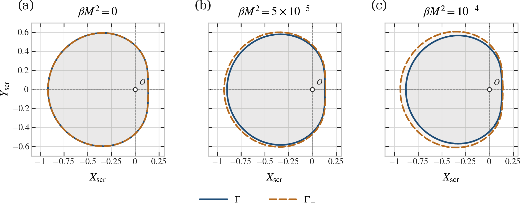
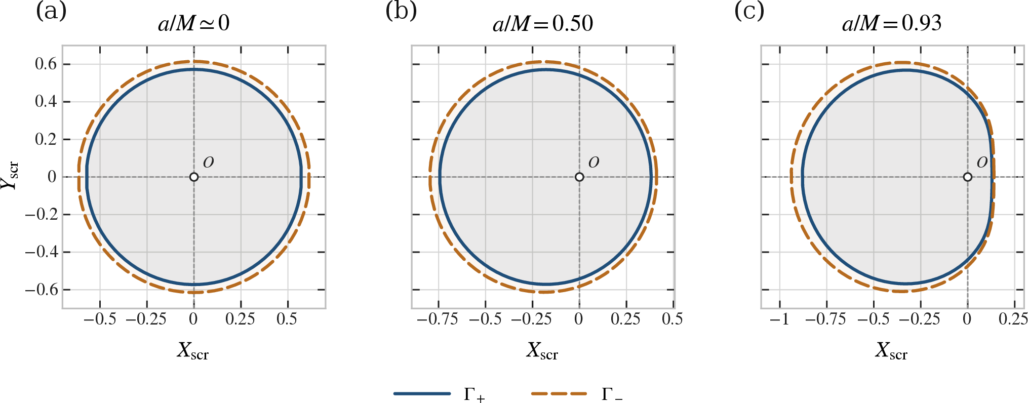
With these quantities, we formally define the critical contour of the optical branch \(s\) on the local celestial sphere as \[\Gamma_s^{\rm cel} := \left\{ \mathbf{n}_s(r_c,\varsigma)\in S^2_o \; ; \; r_c\in\mathcal{I}_s,\; \varsigma=\pm1 \right\}, \qquad s=\pm , \label{eq:Gamma95cel95def95VI}\tag{277}\] and its image on the observer’s stereographic screen as \[\Gamma_s := \left\{ \bigl(X_s(r_c,\varsigma),Y_s(r_c,\varsigma)\bigr) \; ; \; r_c\in\mathcal{I}_s,\; \varsigma=\pm1 \right\}. \label{eq:Gamma95screen95def95VI}\tag{278}\] In what follows, \(\Gamma_s\) will denote the projected contour on the local screen; we will write \(\Gamma_s^{\rm cel}\) only when it is necessary to emphasize the curve on the celestial sphere.

The birefringent comparison is performed on \[\mathcal{I}_{\rm br}:=\mathcal{I}_+\cap\mathcal{I}_-, \label{eq:Ibr95visible95VI}\tag{279}\] where both branches are simultaneously defined. The angular separation between the two branches is measured by \[\Delta_{\rm cel}(r_c,\varsigma) := \arccos \left[ \mathbf{n}_+(r_c,\varsigma)\cdot\mathbf{n}_-(r_c,\varsigma) \right], \qquad r_c\in\mathcal{I}_{\rm br}. \label{eq:Delta95cel95def95VI}\tag{280}\] This quantity is intrinsic to the local celestial sphere and does not depend on the two-dimensional chart used to draw the image. On the stereographic screen, the projected separation between branches is \[\begin{align} \Delta_{\rm scr}(r_c,\varsigma) :={}& \Bigl\{ \bigl[X_+(r_c,\varsigma)-X_-(r_c,\varsigma)\bigr]^2 \\ &+ \bigl[Y_+(r_c,\varsigma)-Y_-(r_c,\varsigma)\bigr]^2 \Bigr\}^{1/2} . \end{align} \label{eq:Delta95scr95def95VI}\tag{281}\] While \(\Delta_{\rm cel}\) measures the intrinsic angular splitting, \(\Delta_{\rm scr}\) describes the separation in the stereographic chart used to visualize the contours.

On this domain we define \[\begin{align} \Delta_{\rm cel}^{\rm max} &:= \max_{\substack{r_c\in\mathcal{I}_{\rm br}\\ \varsigma=\pm1}} \Delta_{\rm cel}(r_c,\varsigma),\\[1mm] \Delta_{\rm scr}^{\rm max} &:= \max_{\substack{r_c\in\mathcal{I}_{\rm br}\\ \varsigma=\pm1}} \Delta_{\rm scr}(r_c,\varsigma) . \end{align} \label{eq:Delta95cel95scr95max95VI}\tag{282}\] The maximum \(\Delta_{\rm cel}^{\rm max}\) is intrinsic to the celestial sphere. By contrast, \(\Delta_{\rm scr}^{\rm max}\) depends on the chosen screen chart and will be used only as a visualization diagnostic. In the Maxwell limit, the two optical roots collapse to the same cone, the critical families coincide, \[\Gamma_+\to\Gamma_-, \qquad \Gamma_+^{\rm cel}\to\Gamma_-^{\rm cel}, \label{eq:Gamma95Maxwell95limit95VI}\tag{283}\] and both splittings vanish.

The previous construction translates the bifurcation of the optical cones into two critical contours on the observer’s local screen. In the linear limit the two branches share the same critical family; away from that limit, the constitutive response separates the optical potentials and produces \(\Gamma_+\neq\Gamma_-\). Figs. 1 and 2 display this separation before it is reduced to global observables. The first figure isolates the role of the nonlinear coupling, whereas the second shows how rotation reorganizes the same geometrical signal.

6.3 Effective diameter and birefringent geometric width↩︎

The separation between \(\Gamma_+\) and \(\Gamma_-\) is not merely a local difference between celestial directions: it affects the full morphology of the projected contour. The maximum \(\Delta_{\rm cel}^{\rm max}\) captures the largest angular separation between branches, but it does not by itself describe the change in global scale or the transverse distribution of the separation. To characterize this global information, we now introduce two screen-based quantities: a relative diameter splitting and an effective geometric width. In horizon-scale image analyses, quantities such as the diameter and the fractional width are used to characterize the observed structure [52], [57]. Here we use their purely geometrical analogues for the critical contours.

We work on the common visibility interval \(\mathcal{I}_{\rm br}\), defined in 279 . For each optical branch \(s=\pm\), we introduce the screen vector \[\begin{align} \mathbf{X}_s(r_c,\varsigma) &:= \bigl(X_s(r_c,\varsigma),Y_s(r_c,\varsigma)\bigr), \\ r_c&\in\mathcal{I}_{\rm br}, \qquad \varsigma=\pm1 . \end{align} \label{eq:Xvector95s95def95VI}\tag{284}\] Scanning \(\mathcal{I}_{\rm br}\), together with the two choices of \(\varsigma\), gives the projected contour \(\Gamma_s\). We assume that the common domain generates closed and regular curves on the screen. If, for a given choice of parameters, only a visible arc is obtained, the same definitions should be understood as restricted to that arc.

The line element on the local screen is defined as \[d\ell_s := \sqrt{dX_s^2+dY_s^2}, \qquad L_s:=\oint_{\Gamma_s}d\ell_s . \label{eq:dells95Ls95def95VI}\tag{285}\] With this measure, the geometrical center of the contour is taken as the arc-length average, \[\mathbf{C}_s := \frac{1}{L_s} \oint_{\Gamma_s} \mathbf{X}_s\,d\ell_s . \label{eq:Cs95def95VI}\tag{286}\] The projected mean radius of the branch \(s\) is defined by \[\bar R_s := \frac{1}{L_s} \oint_{\Gamma_s} \left| \mathbf{X}_s-\mathbf{C}_s \right|\,d\ell_s , \label{eq:Rbar95s95def95VI}\tag{287}\] and the associated effective diameter by \[d_s:=2\bar R_s . \label{eq:ds95def95VI}\tag{288}\] This definition does not assume circularity. For a circular curve it reproduces the usual diameter; for a deformed contour it gives an average size scale on the screen. Thus, \(d_s\) should be understood as a geometrical measure of the critical contour, not as an image diameter already processed by emission, radiative transfer, or instrumental response.

The first global birefringence observable is the relative diameter splitting, \[\delta d_{\rm br} := \frac{2|d_+-d_-|}{d_++d_-}. \label{eq:delta95d95br95def95VI}\tag{289}\] This quantity measures whether the two optical branches, in addition to separating pointwise on the celestial sphere, predict different global scales. In the Maxwell limit, \[d_+\to d_-, \qquad \delta d_{\rm br}\to0 \qquad (\beta\to0). \label{eq:delta95d95br95Maxwell95VI}\tag{290}\]

If the contours \(\Gamma_+\) and \(\Gamma_-\) are too close to be resolved as two separate curves, their separation can be described as a thin band around a mean contour. We define that contour by \[\bar{\mathbf{X}}(r_c,\varsigma) := \frac{1}{2} \left[ \mathbf{X}_+(r_c,\varsigma)+\mathbf{X}_-(r_c,\varsigma) \right], \label{eq:Xbar95def95VI}\tag{291}\] and denote by \(\bar\Gamma\) the curve generated by \(\bar{\mathbf{X}}\). The critical curve is a geometrical object, whereas an observed image depends on the emitting plasma, radiative transfer, and instrumental response; hence the relation between critical curves and observed appearance is not direct [45], [51]. Here we define only the geometrical contribution associated with the separation between the two critical contours.

With line element \[d\bar\ell := \left| d\bar{\mathbf{X}} \right|, \qquad \bar L:=\oint_{\bar\Gamma}d\bar\ell , \label{eq:dellbar95Lbar95def95VI}\tag{292}\] at regular points of the mean contour we define the unit tangent vector \[\hat{\mathbf{t}} := \frac{d\bar{\mathbf{X}}}{\left|d\bar{\mathbf{X}}\right|}, \label{eq:tangent95mean95def95VI}\tag{293}\] and the local oriented normal on the screen, \[\hat{\mathbf{m}} := \bigl(-\hat{t}_Y,\hat{t}_X\bigr). \label{eq:normal95mean95def95VI}\tag{294}\] The separation between the branches is written as \[\delta\mathbf{X}_{\rm br}(r_c,\varsigma) := \mathbf{X}_+(r_c,\varsigma)-\mathbf{X}_-(r_c,\varsigma), \label{eq:deltaX95vector95br95def95VI}\tag{295}\] and its normal component with respect to the mean contour is \[\delta X_\perp(r_c,\varsigma) := \delta\mathbf{X}_{\rm br}(r_c,\varsigma)\cdot\hat{\mathbf{m}}(r_c,\varsigma). \label{eq:deltaX95perp95def95VI}\tag{296}\] This component is the one that contributes to the local geometrical thickness. The tangential component, by contrast, shifts points along the contour and does not by itself produce transverse broadening.

We then define the effective birefringent geometric width by \[w_{\rm br}^2 := \frac{1}{4\bar L} \oint_{\bar\Gamma} \bigl[\delta X_\perp\bigr]^2 \,d\bar\ell . \label{eq:wbr95def95VI}\tag{297}\] The factor \(1/4\) appears because \(\delta X_\perp\) measures the total normal separation between the two branches. If the branches are distributed approximately symmetrically around the mean contour, each branch lies at a distance \(|\delta X_\perp|/2\) from \(\bar\Gamma\). Thus, \(w_{\rm br}\) measures the root-mean-square (rms) half-width induced by birefringence, while \(2w_{\rm br}\) represents the full rms normal separation between the two contours.

To obtain a dimensionless quantity, we normalize this width by the mean diameter \[d_0 := \frac{1}{2}(d_++d_-), \label{eq:d095mean95def95VI}\tag{298}\] and define \[f_{\rm br} := \frac{w_{\rm br}}{d_0}. \label{eq:fbr95def95VI}\tag{299}\] This diagnostic is the geometrical analogue of a fractional width. If the two critical curves are not resolved separately, \(f_{\rm br}\) quantifies the minimum contribution that the separation of the optical cones can make to the effective width of the projected structure. In the linear limit, \[\begin{align} \mathbf{X}_+(r_c,\varsigma)&\to\mathbf{X}_-(r_c,\varsigma), \\ w_{\rm br}&\to0, \qquad f_{\rm br}\to0, \qquad (\beta\to0) . \end{align} \label{eq:fbr95Maxwell95limit95VI}\tag{300}\]

The construction leaves three main geometrical diagnostics: \[\Delta_{\rm cel}^{\rm max}, \qquad \delta d_{\rm br}, \qquad f_{\rm br}. \label{eq:main95geometric95observables95summary95VI}\tag{301}\] The first one measures the maximum local angular splitting and is defined directly on the observer’s celestial sphere. The other two condense the same separation into global screen scales: \(\delta d_{\rm br}\) measures whether the two branches predict different effective diameters, whereas \(f_{\rm br}\) measures the geometrical width associated with an unresolved splitting. By contrast, \(\Delta_{\rm scr}^{\rm max}\) is kept only as a diagnostic of the stereographic chart used to visualize the contours.

To complement the maximum angular separation, which may be sensitive to the endpoints of the visible interval, we also report the discrete average \[\langle\Delta_{\rm cel}\rangle := \frac{1}{N_{\rm br}} \sum_{(r_c,\varsigma)\in\mathcal{I}_{\rm br}^{\rm num}} \Delta_{\rm cel}(r_c,\varsigma). \label{eq:Delta95cel95mean95def95VI}\tag{302}\] Here \(\mathcal{I}_{\rm br}^{\rm num}\) denotes the set of numerical points in the common domain used to trace both branches simultaneously, including the two choices of \(\varsigma\), and \(N_{\rm br}\) is its cardinality. This average does not replace \(\Delta_{\rm cel}^{\rm max}\); it only summarizes the typical size of the angular splitting along the common contour.

To assess the geometrical stability of these diagnostics, we perform three representative scans within the perturbative domain \(\epsilon_{\rm pert}\leq0.05\). In all of them we fix \[M=1,\qquad p=0.2,\qquad q=0.3,\qquad r_o=8,\] and vary, respectively, the nonlinear coupling \(\beta\), the rotation parameter \(a/M\), and the observer inclination \(\theta_o\). The complete numerical values, together with the rationale for the reference dyonic sector, are collected in Appendix 9.

The qualitative reading of these scans is direct. In the Maxwell limit, the contours \(\Gamma_+\) and \(\Gamma_-\) collapse into a single critical curve, and the diagnostics \(\Delta_{\rm cel}^{\rm max}\), \(\delta d_{\rm br}\), and \(f_{\rm br}\) vanish simultaneously. When the nonlinear constitutive response is turned on, the two optical branches generate distinct critical families: \(\beta\) controls the opening between the cones, rotation redistributes the signal over the screen, and inclination changes its local projective realization without removing the splitting.

This completes the geometrical chain constructed in this section. The local constitutive response separates the Fresnel cones; each cone defines an effective optical metric; Carter-type separability allows one to construct branch-dependent critical families; and the local projection maps those families into two screen contours. The contours \(\Gamma_\pm\) are therefore critical curves of the effective optical geometries. They are not luminous rings and do not replace an accretion image; rather, they set the geometrical support on which emission, plasma effects, and radiative transfer can be incorporated in a subsequent step.

7 Physical discussion and scope↩︎

The calculation has a simple physical meaning. The rotating García–Díaz metric gives the gravitational background, but in NLED the propagation of electromagnetic perturbations is not fixed by this metric alone. The perturbation also feels the local constitutive law of the nonlinear electromagnetic field. For this reason the pair \((F,P)\) is not only a technical way to write the solution. It contains the response that fixes the optical cones [10]–[15].

This point is especially useful for the García–Díaz family. The same exact branch contains the metric, the mixed potentials and the constitutive structure of the Einstein–NLED system [81], [82], [85]. Therefore, the optical metrics used in this work are not phenomenological deformations of Kerr or Kerr–Newman. They are obtained from the local response matrix reconstructed from the exact fields. In this sense, the birefringent splitting belongs to the solution itself.

At the perturbative order considered here, the Fresnel quartic factorizes into two quadratic branches. In the Maxwell limit the two branches collapse to the same null cone. When the nonlinear response is active, they define two different effective optical metrics. In the principal tetrad, the deformation acts differently on the temporal–radial and angular blocks, and the tensor \(F^\mu{}_{\alpha}F^{\alpha\nu}\) gives the algebraic direction of the effect. This is the local form of constitutive birefringence.

The next important point is separability. The two optical metrics are not the background metric, but at first order they still keep enough Kerr-type structure to separate the Hamilton–Jacobi equation. Thus each branch has its own radial potential, angular potential, separation constant and critical family. Birefringence therefore does not appear here as a loss of the critical problem. It appears as a doubling of it.

This doubling becomes visible only after projection. In a rotating geometry, the shadow edge is not controlled by one circular orbit. It is controlled by a family of critical orbits and by the way this family is projected on the screen of the observer [39], [46], [68], [70]. Each optical branch produces its own projected contour, \(\Gamma_+\) or \(\Gamma_-\). The separation between these contours is the geometrical imprint of birefringence. We measure it by the maximum angular separation, the relative diameter shift and the normalized geometrical width. These are not flux observables. They are clean geometrical quantities defined before choosing any accretion model.

The Maxwell limit gives a useful check. When \(\beta\to0\), the two Fresnel roots become the same, and the diagnostics \(\Delta_{\rm cel}^{\rm max}\), \(\delta d_{\rm br}\) and \(f_{\rm br}\) all go to zero. Thus the splitting is not produced by the observer tetrad, by the screen coordinates or by a choice of parametrization. It comes from the nonlinear constitutive response.

The use of a finite-distance observer is also part of the construction. For \(\beta\neq0\), the branch is not asymptotically flat in the usual sense, so it is not natural to define the shadow only through impact parameters at infinity. A local orthonormal tetrad gives a well-defined projection of the critical families. This places the construction in the same spirit as finite-distance treatments of shadows and critical curves in rotating geometries [39], [42], [46], [61], [62], [65].

The numerical scans support this interpretation. In the controlled regime \(\epsilon_{\rm pert}\leq0.05\), the splitting grows with the nonlinear coupling. Rotation does not create birefringence by itself, but it redistributes the separation along the projected critical family. Changing the observer inclination modifies the projection, but it does not remove the separation between \(\Gamma_+\) and \(\Gamma_-\). This is why the signal is best understood as constitutive in origin, redistributed by rotation and then seen through the local observer projection.

There is also a useful connection with other NLED observables. The recent study of quasinormal modes in a static Plebański-type NLED black hole showed that the nonlinear electromagnetic sector can affect the dynamical perturbation problem [31]. Here we find the complementary result in geometrical optics: the same type of constitutive structure can also affect the optical cones and the critical contours. These two directions are different, but they share the same physical lesson. In Einstein–NLED systems, the electromagnetic response is not a passive background detail.

The present work is still a geometrical study. The curves \(\Gamma_+\) and \(\Gamma_-\) are critical contours of two effective optical geometries. They are not yet full images produced by an accretion flow. A complete image would require emission, absorption, polarized radiative transfer, plasma effects and instrumental response [47], [51], [52], [54], [57]–[59], [97]–[101]. The role of this paper is to isolate the geometrical support on which such a birefringent image would have to be built.

The final message is therefore direct. NLED does not only change the stress-energy tensor that sources the geometry. In the geometrical-optics limit, it also changes the characteristic structure followed by the electromagnetic perturbation. In the rotating García–Díaz black hole, this change can be followed explicitly from the local constitutive response to the Fresnel cones, the separated optical dynamics and the projected critical contours on the observer screen.

8 Summary and conclusions↩︎

We have studied high-frequency electromagnetic propagation in the rotating García–Díaz black hole of Einstein gravity coupled to NLED. The aim was to follow one complete chain: from the exact mixed potentials of the solution, to the local constitutive response, to the Fresnel optical metrics, and finally to the critical contours seen by a finite-distance observer.

The first step was the reconstruction of the constitutive branch. In the principal tetrad, the electromagnetic sector is described by four aligned scalars, \(E\), \(B\), \(D\) and \(H\). In the Maxwell limit one has \(D=E\) and \(H=B\). For nonzero nonlinear coupling this equality is deformed by the factors \(\kappa_r\) and \(\kappa_\theta\). This allowed us to write the regular branch as a local map \((D,B)\mapsto(E,H)\) and to obtain the response matrix. The optical geometry was then derived from this response; it was not assumed independently.

The second step was the Fresnel construction. At the perturbative order used here, the Fresnel quartic splits into two quadratic branches. In the Maxwell limit these branches become the same light cone. Away from that limit, they define two effective optical metrics. The deformation is controlled by the quadratic tensor of the background electromagnetic field, and it distinguishes the temporal–radial block from the angular block in the principal tetrad.

The third step was the separability analysis. Although the optical metrics differ from the spacetime metric, both branches admit a Carter-type separation at first order. For each branch \(s=\pm\), one can define a radial potential, an angular potential, critical constants and a family of unstable critical orbits. Thus the nonlinear response does not remove the integrable structure at this order. Instead, it produces two branch-dependent copies of the critical problem.

The fourth step was the local projection. Since the branch is not asymptotically flat for \(\beta\neq0\), we projected the critical families on the celestial sphere of a finite-distance observer. This gives two contours, \(\Gamma_+\) and \(\Gamma_-\). They coincide when \(\beta=0\) and separate when the NLED response is active. We quantified the separation by the maximum angular distance between the contours, the relative diameter shift and the normalized birefringent width. These quantities isolate the geometrical part of the effect before any emission model is introduced.

The numerical scans give the same picture in a more concrete way. Increasing \(\beta\) opens the two branches. Rotation redistributes the separation on the screen, without being the source of birefringence by itself. Changing the observer inclination changes the projection, but the two-contour structure remains. In the Maxwell limit all the diagnostics vanish at the same time. This confirms that the splitting is not a coordinate or projection artifact; it is produced by the constitutive response of the nonlinear electromagnetic sector.

The main conclusion is that the rotating García–Díaz solution gives a clear example where the internal electromagnetic response of an Einstein–NLED black hole reaches the observable critical geometry. A local property of the field–excitation relation becomes a splitting of the optical cones, then a splitting of the critical families, and finally a separation between two projected contours on the observer screen.

Several extensions are natural. The first one is to include emission and polarized radiative transfer on the two optical branches, in order to see how \(\Gamma_+\) and \(\Gamma_-\) would be illuminated in synthetic images. A second one is to go beyond the perturbative optical reconstruction and test the birefringent structure with direct numerical integration of the effective characteristics. A third one is to compare this rotating branch with static and other Einstein–NLED solutions, so that one can separate the effects of rotation, constitutive anisotropy and strong gravity.

Overall, the result shows that a rotating Einstein–NLED solution can keep enough separable structure to allow analytic control, while at the same time producing a genuine birefringent splitting of the critical contours. This is the central point of the paper: the local constitutive response can be carried, in a controlled way, all the way to geometrical diagnostics on the observer screen.

Code and data availability↩︎

The computational material associated with this work is available in the companion repository [102]. It contains the notebook and numerical outputs used to reproduce the figures, tables and parameter scans reported in Appendix 9.

9 Numerical control of the birefringent splitting↩︎

This appendix presents the numerical control of the geometrical diagnostics introduced in Sec. 6. Its purpose is to document how the splitting between the critical families \(\Gamma_+\) and \(\Gamma_-\) behaves under representative variations of the nonlinear coupling, the rotation, and the observer inclination. In this way, the tables complement the analytical construction of the main text without interrupting its development.

In all scans we fix \[M=1, \qquad p=0.2, \qquad q=0.3, \qquad r_o=8, \label{eq:app95fixed95parameters}\tag{303}\] and retain only configurations satisfying \[\epsilon_{\rm pert}\leq0.05 . \label{eq:app95epsilon95bound}\tag{304}\] This restriction keeps the calculation within the domain where the perturbative approximation to the optical metrics remains controlled.

The choice of a fixed dyonic sector is deliberate. In this branch, the charges enter the radial function through \(Q_c^2=p^2+q^2\) and also set the constitutive scale appearing in the optical cones. The linear fields \(E_0\) and \(B_0\) are homogeneous of degree one in \((p,q)\), whereas the perturbative optical coefficients contain the factor \(1/Q_c^2\). Therefore, under a common rescaling \((p,q)\to\lambda(p,q)\), the products \(\nu_sE_0^2\) and \(\nu_sB_0^2\), which control the local deformation of the optical metrics, remain invariant at fixed geometry. The remaining effect of varying the total charge scale is mainly channeled through \(\Delta(r)\), the horizon position, the perturbative domain, and the visible portion of the critical families. For this reason, the tables fix a representative dyonic sector and separate three effects more directly: the scan in \(\beta\) isolates the constitutive opening, the scan in \(a/M\) displays the rotational redistribution, and the scan in \(\theta_o\) measures the dependence on the local projection.

In the tables, the maximum angular separation \(\Delta_{\rm cel}^{\rm max}\) and the discrete average \(\langle\Delta_{\rm cel}\rangle\) are shown multiplied by \(10^4\). The relative diameter shift \(\delta d_{\rm br}\) and the normalized width \(f_{\rm br}\) are shown multiplied by \(10^2\). The quantity \(\Delta_{\rm scr}^{\rm max}\) is kept as a diagnostic of the stereographic chart used to visualize the contours, while \(d_0\) and \(w_{\rm br}\) are reported in the geometrical units of the local screen.

9.1 Constitutive opening↩︎

The first scan varies the nonlinear coupling while keeping \(a/M=0.93\) and \(\theta_o=85^\circ\) fixed. This scan isolates the role of the constitutive response. In the Maxwell limit the two branches collapse into a single contour, whereas for \(\beta\neq0\) a geometrical separation between \(\Gamma_+\) and \(\Gamma_-\) appears. Table [tab:app95beta95scan95geometric] shows this behavior directly: all birefringent diagnostics vanish for \(\beta=0\), and then grow as the nonlinear coupling is increased.

9.2 Rotational redistribution↩︎

The second scan varies \(a/M\) while keeping \(\beta M^2=10^{-4}\) and \(\theta_o=85^\circ\) fixed. This scan does not measure the generation of birefringence, which is already present for \(\beta\neq0\), but rather how rotation redistributes the signal on the local screen. As shown in Table [tab:app95spin95scan95geometric], the constitutive response already separates the branches in the nonrotating limit. When the spin is changed, the visible critical family changes its shape and location, so the maximum separation does not need to be monotonic, while the global scale of the splitting remains comparable.

9.3 Observer-projection dependence↩︎

The third scan varies the observer inclination while keeping \(a/M=0.93\) and \(\beta M^2=10^{-4}\) fixed. The background geometry and the two effective optical metrics are unchanged; only the way in which the observer cuts and projects the critical families changes. Table [tab:app95inclination95scan95geometric] shows that the splitting is not tied to a special observer orientation. The projection changes with \(\theta_o\), but the separation between \(\Gamma_+\) and \(\Gamma_-\) remains. Taken together, the three scans show that the signal is opened by the constitutive response, reorganized by rotation, and preserved under changes of local projection inside the perturbative domain considered.

References↩︎