Norms, overlaps and Yangian descendants for the Haldane--Shastry spin chain
June 18, 2026
Norms, overlaps and Yangian descendants
for the Haldane–Shastry spin chain
Yunfeng Jiang1,2, Jules Lamers3, Yuan Miao4 \(\curvearrowright\) 5 \(\diamond\)
1 School of Physics & Shing-Tung Yau Center, Southeast University,
Nanjing 211189, P. R. China
2 Peng Huanwu Center for Fundamental Theory, Hefei, Anhui 230026, P. R. China
3 School of Mathematics and Statistics, University of Glasgow
University Place, Glasgow G12 8QQ, UK
4 Kavli Institute for the Physics and Mathematics of the Universe (WPI),
UTIAS, The University of Tokyo, Kashiwa, Chiba 277-8583, Japan
5 Laboratoire de Physique de l’École Normale Supérieure, ENS, Université PSL, CNRS, Sorbonne Université, Université Paris Cité, Paris, France
\(\diamond\) yuan.miao.physics@gmail.com
2026-06-27
Abstract↩︎
The Haldane–Shastry spin chain is a prototypical integrable model with long-range interactions, notable for hosting quasiparticles with fractional statistics and serving as a discrete analogue of a conformal field theory. Its remarkable simplicity is closely tied to a full Yangian spin symmetry. While the highest-weight states for this symmetry are known explicitly, a systematic treatment of the descendant states, needed for the computation of various physical quantities, has remained incomplete. In this work, we provide a detailed construction of these descendants in terms of the algebraic Bethe ansatz following recent work of Ferrando et al. In the limit of extreme twist, it includes the Gelfand–Tsetlin basis. As an application, we derive product and determinant formulae for norms and overlaps of these states.
1 Introduction↩︎
The Haldane–Shastry (HS) spin chain [1], [2] is the prototypical example of an integrable long-range interacting spin chain. It possesses many remarkable properties, such as hosting quasiparticles with fractional statistics. It has intimate connections with 2-dimensional conformal field theories, and in particular can be viewed as a discrete version of the level-1 \(\mathfrak{su}_2\) Wess–Zumino–Witten model [3]–[7].
While one would generally expect a model with long-range interactions to be more complicated than spin chains with nearest-neighbour interactions, the HS chain is in fact in some respects simpler than the Heisenberg xxx chain. Indeed, the HS chain is not just exactly but even explicitly solvable: its eigenvalues and (certain) eigenvectors can be written in a simple, closed form [8]–[10]. This simplicity also shows up in an enlarged spin symmetry: the Hamiltonian is invariant under the full Yangian [9], [10], which contains the standard \(\mathfrak{su}_2\) spin symmetry algebra as a subalgebra. The monodromy matrix for the HS chain is different from the one of the Heisenberg xxx chain [9], [10], and the Hamiltonian comes from expansions of the so-called quantum determinant. Thanks to this Yangian symmetry, the Hilbert space of the HS chain decomposes into several Yangian multiplets (irreducible representations) that are the eigenspaces of the HS Hamiltonian. As a consequence, the HS chain has high degeneracies, as was already observed in [1]. The Yangian highest-weight (yhw) states, also known as pseudovacua, of these multiplets have been studied extensively [9], [10], and their wave functions are given explicitly in terms of Jack polynomials (see Sec. 2 for details). Together, the explicit yhw states and the Yangian symmetry in principle determine all eigenstates. However, the monodromy matrix of the HS chain is complicated, requiring one to work with the more general setting of spin-Calogero–Sutherland systems, from which the HS chain is obtained by a process called freezing [10]. Perhaps for this reason, the remaining (Yangian descendant) eigenstates have received less attention, having only been mentioned briefly in various places [3], [10]–[12]. In order to study out-of-equilibrium dynamics and finite-temperature properties of the HS chain, which require sums over all states in the Hilbert space, a better understanding of the Yangian descendants is required.
The goal of this paper is to determine the norms and overlaps of the yhw and descendant states, paving the way for the study of various important physical properties, including the correlation functions and out-of-equilibrium dynamics.
Since this monodromy matrix commutes with the HS Hamiltonian, one cannot use conventional Bethe-ansatz techniques in the same way as for the Heisenberg xxx chain. Instead, each HS eigenspace has, like any finite-dimensional Yangian multiplet, the structure of an ‘effective’ inhomogeneous Heisenberg chain with special, fixed inhomogeneities depending on the eigenspace. Building on [11], in [12] it was proposed to study the complete eigenbasis using an ‘internal Bethe ansatz’ inside each eigenspace separately, by diagonalizing the HS Hamiltonian simultaneously with the transfer matrix. This allows one to leverage the powerful toolkit of traditional Heisenberg-style integrability per eigenspace. Notably, the joint eigenstates are given by the algebraic Bethe ansatz (aba), leading to Bethe-ansatz equations (bae) for each eigenspace, or, equivalently, \(TQ\)-relations. When the parameters in the aba are ‘on shell’, i.e.solve the bae, the Bethe states become eigenstates of the transfer matrix. Considering the (diagonally) twisted transfer matrix \(\mathbf{T}(x; \kappa) = \kappa \, \mathbf{A}(x) + \kappa^{-1} \, \mathbf{D}(x)\), this yields a description of the descendants as an eigenbasis depending on the value of the twist \(\kappa\), orthogonal in the regime of \(\kappa\) where the transfer matrix is hermitian. Among all possible twists, two choices are special:
in the periodic case \(\kappa=1\), the effective spin chain has \(\mathrm{SU}(2)\) symmetry;
in the limits \(\kappa\to 0\) or \(\kappa\to\infty\) of extreme twist, the Bethe roots become explicit, and the Bethe vectors reduce to the so-called Gelfand–Tsetlin basis [13]–[16].
The aba allows one to compute the overlaps of descendant states, which are orthogonal when the transfer matrix is hermitian and have norms given by the Gaudin determinant [17]–[20]. Furthermore, overlaps of one ‘on-shell’ and one ‘off-shell’ Bethe state are given by the Slavnov determinant formula [20], [21].
Our main results are as follows. The ‘quantum numbers’ labelling the eigenspaces of the HS chain are called ‘motifs’, see Sec. 2.2. Their yhw states are known explicitly, see Sec. 2.4. In Sec. 4.4, we use the orthogonality of Jack polynomials to prove that the yhw states for different motifs \(\mu\) are orthogonal (despite ‘accidental’ degeneracies of the HS chain), and that the yhw state \(\ket{0}_{\mu}\) for the motif \(\mu\) has norm-squared given by the simple factorised formula \[\label{eq:normHigh} {_{\mu}}\braket{0}{0}_{\mu} = N^M \prod_{m < m'}^M \frac{\mu_m -\mu_{m'}-1}{\mu_m - \mu_{m'} + 1} \; ,\tag{1}\] where \(M\) is the number of down spins in \(\ket{0}_{\mu}\). In Sec. 4.1 we obtain Yangian descendant states by diagonalising the twisted transfer matrix in the Yangian multiplet labelled by \(\mu\) using the aba \(\ket{\boldsymbol{{u}}}_{\mu} \mathrel{\vcenter{:}}= \mathbf{B}(u_1)\cdots \mathbf{B}(u_K)\,\ket{0}_\mu\), leading to the bae 47 . In Sec. 4.4 we show that the norm of Yangian descendant states is proportional to the Gaudin determinant \(G_{\boldsymbol{{u}}, \boldsymbol{{u}}}\) given in 57 , \[\frac{{_\mu}\braket{\boldsymbol{{u}}}{\boldsymbol{{u}}}_{\mu}}{{_\mu}\braket{0}{0}_{\mu} } = \biggl( \, \prod_{k=1}^K A_\mu (u_k) \, D_\mu (u_k) \biggr) \, G_{\boldsymbol{{u}}, \boldsymbol{{u}}} \; ,\] while the overlap between on-shell and off-shell Yangian descendants (within the same Yangian multiplet) is proportional to the Slavnov determinant \(S_{\boldsymbol{{v}}, \boldsymbol{{u}}}\) from 56 , \[\frac{{_\mu}\braket{\boldsymbol{{v}}}{\boldsymbol{{u}}}_{\mu}}{{_\mu}\braket{0}{0}_{\mu}} = \delta_{K,K'} \Biggl( \, \prod_{k=1}^K A_\mu (v_k) \, D_\mu (u_k) \Biggr) \, S_{\boldsymbol{{v}}, \boldsymbol{{u}}} \; ,\] with proportionality factors containing polynomials \(A_\mu (x)\) and \(D_\mu (x)\) that are given in 39 –40 .
The rest of the paper is structured as follows. In Sec. 2, we review various known properties of the HS chain and present our main results in more detail (see the end of Sec. 2.4, and Sec. 2.5). The proofs of these results are given in the subsequent two sections. In Sec. 3, we review the relationship between the HS chain and the spin Calogero–Sutherland system through ‘freezing’, and explain how to formulate the aba for the HS chain using ‘frozen’ Dunkl operators. Equipped with this formalism, we show in Sec. 4 how to construct Yangian descendant states via the aba technique. Then we discuss the special values of the twist, and derive the norm and overlap formulae. To illustrate our results, we present explicit examples in Sec. 5. We conclude and discuss future directions in Sec. 6. In addition, there are two appendices: App. 7 contains the Yangian relations for the quantum operators for easy reference, and App. 8 contains the basics of the inhomogeneous Heisenberg chain and TQ relations.
2 Overview: old, and some new, results for Haldane–Shastry↩︎
We start with the Hilbert space \((\mathbb{C}^2)^{\otimes N}\) for \(N\) sites with spin \(1/2\), and use the standard notation for local operators, e.g.\(\mathbf{O}_j = \mathbb{I}^{\otimes (j-1)} \otimes \mathbf{O} \otimes \mathbb{I}^{\otimes (N-j)}\). In particular, \(\sigma^\alpha_j\) denotes the \(\alpha\)th Pauli matrix acting locally at the \(j\)th site. The permutation operator can be defined as \[\label{eq:perm} \mathbf{P}_{ij} = \frac{1}{2} \left( 1 + \vec{\sigma}_i \cdot \vec{\sigma}_j \right) \, ,\tag{2}\] such that \(\mathbf{P}_{ij} \, \mathbf{O}_i = \mathbf{O}_j \, \mathbf{P}_{ij}\) and \(\mathbf{P}_{ij}^2 = 1\). The Haldane–Shastry spin chain is defined by the Hamiltonian \[\label{eq:H95HS} \mathbf{H}_\mathrm{\small hs} = \sum_{i < j}^N \frac{1 - \mathbf{P}_{ij}}{4 \sin^2\bigl(\pi (i - j)/N\bigr)} \; .\tag{3}\]
2.1 Conserved charges↩︎
The HS chain has two types of conserved charges. There are \(N\) ‘basic’ charges, containing the translation operator (or momentum) and Hamiltonian [9], [22], [23]. These commute with all Yangian generators; from the Yangian perspective, these charges are generated by the quantum determinant [10]. Higher conserved charges can be derived systematically [23]. For instance, \[\begin{align} \mathbf{Q}_3 = &\,\sum_{\substack{i,j,k=1\\ i\neq j\neq k}}^{N} \frac{\mathbf{P}_{ij} \, \mathbf{P}_{jk}}{\sin\bigl[\frac{\pi}{N}(i-j)\bigr] \, \sin\bigl[\frac{\pi}{N}(j-k)\bigr] \, \sin\bigl[\frac{\pi}{N}(k-i)\bigr]} \; ;\\ \mathbf{Q}_4 = &\,\sum_{\substack{i,j,k,l=1\\ i\neq j\neq k\neq l}}^N \frac{\mathbf{P}_{ij} \, \mathbf{P}_{jk} \, \mathbf{P}_{kl}}{\sin\bigl[\frac{\pi}{N}(i-j)\bigr] \, \sin\bigl[\frac{\pi}{N}(j-k)\bigr] \, \sin\bigl[\frac{\pi}{N}(k-l)\bigr] \, \sin\bigl[\frac{\pi}{N}(l-i)\bigr]}\\ & \quad - 2\sum_{\substack{i,j=1\\ i\ne j}}^N \frac{\mathbf{P}_{ij}}{\sin^4\bigl[\frac{\pi}{N}(i-j)\bigr]} \; . \end{align}\] The literature on the HS chain has traditionally focussed on these commuting charges possessing Yangian symmetry.
On top of this, one can construct additional charges [12], [24]. In [12], ‘Heisenberg-style’ charges were constructed that depend on a twist parameter, and commute with each other and the ‘basic’ charges, but not with all Yangian generators. They arise from a twisted transfer matrix, \(\mathbf{T}(x; \kappa) = \kappa \, \mathbf{A}(x) + \kappa^{-1} \, \mathbf{D}(x)\), in analogy to the Heisenberg xxx chain. An explicit example of such a Heisenberg-style charge for arbitrary twist \(\kappa\) is \[\label{eq:Heis95style} \frac{\kappa + \kappa^{-1}}{2} \, \sum_{i<j}^N \mathbf{P}_{ij} + \frac{\kappa - \kappa^{-1}}{4\,\mathrm{i}} \, \sum_{i<j}^N \frac{\mathrm{e}^{\mathrm{i}\pi(i-j)/N} \, \sigma^z_j - \mathrm{e}^{\mathrm{i}\pi(j-i)/N} \, \sigma^z_i}{\sin\bigl[\frac{\pi}{N}(i-j)\bigr]} \, \mathbf{P}_{ij} \, .\tag{4}\] At \(\kappa=1\) this reduces to the total spin operator (quadratic Casimir). In that case, a nontrivial example is \[\label{eq:Heis95style95isotr} \sum_{\substack{i,j,k=1\\ i\neq j\neq k}}^{N} \biggl( \frac{1}{3} + \mathrm{i}\,\cot\Bigl[\frac{\pi}{N}(i-j)\Bigr]\biggr) \, \mathbf{P}_{ij} \, \mathbf{P}_{jk} \, .\tag{5}\] The presence of these additional charges is related to superintegrability. For more, see [12].
2.2 Motif description of the spectrum: eigenvalues↩︎
The spectrum of the HS chain can be described conveniently by simple combinatorial objects called motifs. A motif is a sequence \(\mu =(\mu_1,\ldots,\mu_M)\) of integers satisfying the exclusion rule [1] \[\label{eq:motifs} \mu_{m+1} > \mu_m + 1 \, , \qquad 1\leqslant \mu_m\leqslant N-1 \, ,\tag{6}\] where \(N\) is the length of the spin chain. Motifs label eigenspaces.
When we consider the complete eigenbasis of the HS chain, it will be useful to have a notation for the set of all motifs. We write \(\mathcal{M}_N\) for the set of all motifs for a chain of length \(N\). For example: \(\mathcal{M}_2=\{\varnothing, (1 ) \}\), \(\mathcal{M}_3=\{\varnothing, (1), (2 ) \}\), \(\mathcal{M}_4=\{\varnothing, (1), (2), (3), (1,3) \}\). Note that \(\mathcal{M}_{N-1} \subset \mathcal{M}_N\). The motifs in \(\mathcal{M}_N \setminus \mathcal{M}_{N-1}\) are precisely those obtained by appending the integer \(N-1\) to every motif in \(\mathcal{M}_{N-2}\). This recursion implies that the number of motifs follows a Fibonacci sequence, \(\{\#\mathcal{M}_N\}_{N\geqslant 2} = \{2, 3, 5, 8, 13, \ldots\}\).
2.2.0.1 Energy and momentum.
Consider the rescaled motif \[\label{eq:p95m} p_m = \frac{2\pi}{N} \, \mu_m \, , \qquad m = 1,\dots,M\,.\tag{7}\] Then the eigenspace associated with the motif \(\mu = (\mu_1, \dots, \mu_M)\in\mathcal{M}_N\) has (total) momentum \(p(\mu)\) and energy \(E(\mu)\) given in terms of the motif as \[\label{eq:EP} p(\mu)= \sum_{m=1}^M p_m \;\, \mathrm{mod}\;2\pi \; , \quad E(\mu)= \sum_{m=1}^M \varepsilon(p_m)\; ,\tag{8}\] where the dispersion relation is \[\label{eq:disperseRel} \varepsilon(p_m) = \frac{N^2}{8\pi^2} \;p_m \, (2\pi - p_m) \;.\tag{9}\]
Thanks to 8 , the \(p_m\) from 7 can be interpreted as on-shell quasimomenta of the quasiparticles (magnons). According to 7 , all quasimomenta are real for yhw states. Their values are exactly quantised as for free particles on a circle, with the motif rule 6 a generalised Pauli principle enforcing a fractional (exclusion) statistics [8].
Since the dispersion 9 is quadratic and the energies 8 are additive even on shell, the spectrum of the HS chain is extremely simple: the energies are fully explicit and, up to an overall normalisation, take integer values. This stands in contrast to typical Bethe-ansatz solvable models, such as the Heisenberg chain, where solving the bae is non-trivial and the spectrum generally lacks a closed-form expression.
2.2.0.2 Comparison to BAE.
Consider for a moment quasimomenta \(p_m\) satisfying the following Bethe-ansatz-like equations [8], [25] \[\label{eq:simpleBAE} N \,p_m = 2\pi \, I_m + 2\pi \!\! \sum_{\substack{n=1 \\ n \neq m}}^M \! \mathrm{sgn}(p_m - p_n) \; ,\tag{10}\] where the quantum numbers \(I_m\) take ascending values in \(\{\frac{M+1}{2}, \frac{M+3}{2}, \dots, N-\frac{M+1}{2}\}\).
From 10 , the scattering phase between quasiparticles is nearly trivial, \(S(p_m, p_n) = e^{\mathrm{i}\,\pi\,\text{sgn}(p_m - p_n)} = -1\), indicating a ‘free spectrum’1. The solutions to 10 are \[p_m = \frac{2\pi}{N} \left( I_m +m - \frac{M+1}{2} \right) \; ,\] with quantum numbers \(I_m\) in an ascending order. Defining \(\mu_m = I_m +m - (M+1)/2\) we are led to integers increasing according to the exclusion rule 6 . Thus, the motifs can be viewed as an analogue of Bethe quantum numbers in the Heisenberg chain.
We stress that 10 are not Bethe-ansatz equations in the usual sense, in that they do not follow from the periodicity of any Bethe-ansatz type wave function. However, 10 do arise as the long-range limit of the asymptotic Bethe ansatz equations of the Inozemtsev spin chain as \(N\to \infty\), cf. §4.4 of [28].
2.3 Yangian symmetry↩︎
Each motif is in general associated with more than one eigenstate, i.e.the spectrum is degenerate. This degeneracy arises from the underlying symmetry of the model. For the HS chain, the degeneracies are much larger [1] than one would expect based on the form of the Hamiltonian 3 .
Clearly, the HS chain is isotropic: the Hamiltonian commutes with the \(\mathfrak{su}_2\) generators \[\begin{align} \label{eq:Salpha} \mathbf{S}^{\alpha}=\frac{1}{2}\sum_{j=1}^N\sigma_j^{\alpha} \, ,\qquad \alpha\in \{ x,y,z\} \; . \end{align}\tag{11}\] In fact, the model has much more spin symmetry, which turns out to be governed by the following algebraic object.
2.3.0.1 Yangian symmetry.
The Yangian is an infinite-dimensional quantum group generated by the 11 together with a second set of ‘affine generators’. For the HS chain, they are given by [9] (see also [4], [29]) \[\begin{align} \label{eq:Qalpha} \mathbf{Q}^{\alpha} = \sum_{i<j}^N \cot\biggl(\frac{\pi}{N}(i-j)\biggr) \left(\vec{\sigma}_i\times\vec{\sigma}_j\right)^{\alpha} \, ,\qquad \alpha\in \{ x,y,z\} \; . \end{align}\tag{12}\] These bilocal operators form an adjoint representation of \(\mathfrak{su}_2\), \[\begin{align} \left[ \mathbf{S}^{\alpha}, \mathbf{Q}^{\beta} \right]=\sum_{\gamma \in \{ x,y,z\}} 2 \, \mathrm{i} \, \epsilon^{\alpha\beta\gamma} \, \mathbf{Q}^{\gamma} \; , \end{align}\] and obey additional Serre-type relations [16], [30]. Higher Yangian generators are obtained from repeated commutators of \(\mathbf{Q}^{\alpha}\).
Like the spin operators 11 , the generators 12 are symmetries of the HS chain [9], [10]: \[[\mathbf{S}^{\alpha},\mathbf{H}_\mathrm{\small hs}] = [\mathbf{Q}^{\alpha},\mathbf{H}_\mathrm{\small hs}] = 0 \, .\] Due to this large amount of symmetry, the Hilbert space decomposes into eigenspaces that form Yangian multiplets, i.e.irreducible highest-weight representations of the Yangian. Each such eigenspace is labelled by a motif.
Other sets of generators for the Yangian are available as well. This in particular includes the monodromy matrix[10], whose construction for the HS chain we will review in Sec. 3. This gives access to the framework of the Quantum Inverse Scattering Method (QISM), which we will exploit in Sec. 4.
2.3.0.2 Degeneracies.
Finite-dimensional \(\mathfrak{su}_2\)-multiplets are characterised by their (total) spin \(s\,(s+1)\), or equivalently by the (half-integer) spin \(s\), for a multiplet of dimension \(2\,s+1\). Similarly, any finite-dimensional Yangian multiplet is characterized by a quantity called the ‘Drinfeld polynomial’ (cf.[16]), which is a polynomial in the spectral parameter. For the multiplet labelled by a motif \(\mu \in \mathcal{M}_N\), the Drinfeld polynomial is [10], [31] \[P_\mu(x) = \! \prod_{\substack{n = 1 \\ n \notin \mu \cup (\mu +1)}}^N \!\!\!\!\!\!\!\! \biggl(x + \frac{N+1-2\,n}{2} \biggr) \; , \label{eq:Drinfeldpoly}\tag{13}\] where we introduced the ‘thickened motif’ \(\mu \cup (\mu +1) = ( \mu_1,\mu_1 + 1,\dots,\mu_M , \mu_M +1 )\).
In particular, the Drinfeld polynomial determines the dimension of the multiplet. This works as follows, see e.g. [32]. The zeroes of any Drinfeld polynomial can be organized into ‘strings’.2 By definition, an ‘\(\ell\)-string’ is a maximal set of consecutive zeroes \(\{ z , z+1 , \dots, z+\ell-1 \}\) of the Drinfeld polynomial. For 13 associated to the motif \(\mu\), defining \(\mu_0=-1\) and \(\mu_{M+1} = N+1\), the strings of zeroes \(\{ \mu_{m} +2 -\tfrac{N+1}{2} , \dots , \mu_{m+1} -1 -\tfrac{N+1}{2}\}\) (possibly empty) with \[\label{eq:string95lengths} \ell_m = \mu_{m+1} - \mu_m -2 \; , \qquad m = 0 , 1 , \dots , M\; ,\tag{14}\] In terms of usual spin multiplets, each \(\ell_m\)-string corresponds to a spin-\(\frac{\ell_m}{2}\) irrep of \(\mathfrak{sl}_2\). In particular, a 0-string corresponds to a singlet (trivial representation). The full Drinfeld polynomial corresponds to the tensor-product representation whose factors have spins \(\frac{\ell_0}{2}, \frac{\ell_1}{2}, \dots, \frac{\ell_M}{2}\) in terms of \(\mathfrak{sl}_2\). Thus, by 13 the degeneracy of the multiplet labelled by the motif \(\mu\) is \[\label{eq:dimensionmu} \begin{align} \text{dim}(\mu) = \prod_{m=0}^{M} \! ( \ell_m +1 ) = \left\{\begin{array}{ll} N+1 &\text{if }\mu=\varnothing \; ,\\ \displaystyle \mu_1 \, (N-\mu_M)\prod_{m=1}^{M-1}(\mu_{m+1}-\mu_m-1) &\text{if }M\geqslant 1 \; . \end{array}\right. \end{align}\tag{15}\] While the multiplet is irreducible for the Yangian, as soon there is more than one \(\ell\)-string, for \(\mathfrak{sl}_2\) it decomposes into several spin multiplets, via the usual Clebsch–Gordan decomposition. We will give some examples of this in Sec. 5.
In particular, since adding the dimensions 15 (number of linearly independent Yangian descendants) for all motifs \(\mu \in \mathcal{M}_N\) (labelling different eigenspaces) gives the dimension \(2^N\) of the whole HS Hilbert space, the preceding description of the energy spectrum is complete.
Each Yangian multiplet consists of a Yangian highest-weight state and its descendants, which we will discuss in turn.
2.4 Yangian highest-weight states↩︎
Each eigenspace, labelled by some motif \(\mu\), contains a unique Yangian highest-weight (yhw) state, or pseudovacuum, \(\ket{0}_\mu\).
2.4.0.1 Explicit form.
For a motif \(\mu = (\mu_1,\dots,\mu_M)\) the yhw state has magnon number (number of \(\downarrow\)s) equal to \(M\). For instance, for the empty motif \(\mu=\varnothing\) the vector \(\ket{0}_\varnothing = \ket{{\uparrow}\cdots \uparrow}\) is the ferromagnetic yhw state.
In the coordinate basis, defined by \[\begin{align} \label{eq:coord95basis} \cket{ n_1, \ldots, n_M } \mathrel{\vcenter{:}}= \sigma_{n_1}^- \cdots \sigma_{n_M}^- \ket{\uparrow \cdots \uparrow} \; , \end{align}\tag{16}\] the \(M\)-magnon yhw state \[\begin{align} \ket{0}_{\mu} = \sum_{n_1 < \cdots < n_M}^N \!\!\!\!\! \Psi_{\mu}(n_1, \ldots, n_M) \, \cket{ n_1, \ldots, n_M } \label{eq:Y95hw} \end{align}\tag{17}\] labelled by the motif \(\mu\) has explicit wave function [8] \[\Psi_{\mu} (n_1, \dots , n_M) = \omega^{n_1} \cdots \omega^{n_M} \, V( \omega^{n_1} , \dots, \omega^{n_M})^2 \; \mathsf{P}_{\nu(\mu)} (\omega^{n_1} , \dots, \omega^{n_M}) \; . \label{eq:Y95hw95wf}\tag{18}\] The right-hand side is a product of polynomials in \(M\) variables that are ‘evaluated’ at roots of unity \(\omega^n = \mathrm{e}^{2\pi \mathrm{i}\mspace{1mu} n/N}\). The first part of 18 , including the Vandermonde determinant \[V(z_1, \dots, z_M) = \, \det\limits_{1\leqslant m,m'\leqslant M} \mathopen{\scalerel*[5.5pt]{\Big(}{ \ensurestackMath{\addstackgap[1.5pt]{\big(}}}} z_{m}^{M-m'} \mathclose{\scalerel*[5.5pt]{\Big)}{ \ensurestackMath{\addstackgap[1.5pt]{\big)}}}}= \prod_{m<m'}^M \!\! ( z_{m} - z_{m'} ) \, ,\] is a Slater–Jastrow wave function multiplied by Marshall signs, \[\label{eq:SlaterJastrow} \omega^{n_1} \cdots \omega^{n_M} \, V( \omega^{n_1} , \dots, \omega^{n_M})^2 = (-1)^{M(M-1)/2} \, \mathrm{e}^{\frac{2\pi \mathrm{i}M}{N}\sum_m n_m} \! \prod_{m<m'}^M \!\! 4 \sin^2 \Bigl( \frac{\pi}{N} (n_m - n_{m'}) \Bigr)\; .\tag{19}\] Next, \(\mathsf{P}_\nu(z_1, \dots, z_M)\) denotes a Jack polynomial with parameter \(\alpha = 1/2\) (also known as a spherical zonal polynomial) and partition \(\nu = \nu(\mu)\) determined by the motif through 3 \[\nu_m = \mu_{M -m+1} - 2 \, (M - m) -1 \; , \quad m \in \{1,2,\cdots , M \} \; . \label{eq:nu95from95mu}\tag{20}\]
For motifs of the form \(\mu = (1,3,\dots,2M-1)\), \(\nu(\mu)=0\) and \(\mathsf{P}_\nu(z_1, \dots, z_M)=1\). In particular, when \(N\) is even, the antiferromagnetic ground state at the equator \(M=N/2\) (labelled by the ‘fully packed’ motif \(\mu = (1,3,\dots,N-1)\)) has Slater–Jastrow wave function. This remarkably simple ground state, reminiscent of the fractional quantum Hall effect, is a wave function of the HS chain by design [1], [2]. More about Jack polynomials can be found in e.g. [33].
Other explicit examples and properties of these wavefunctions can be obtained from e.g.§1.1.3 of [31].
2.4.0.2 Orthogonality and norms.
The orthogonality of the yhw states is guaranteed by the properties of Jack polynomials: for any two motifs \(\mu,\mu' \in \mathcal{M}_N\) with cardinality \(M\) and \(M'\), respectively, we prove in Sec. 4.4 that \[\begin{align} \label{eq:pseudo95orthog} {}_{\mu}\braket{0}{0}_{\mu'} & = \delta_{M,M'} \!\! \sum_{n_1 < \dots < n_M}^N \!\!\! \bigl| \Delta (\omega^{n_1}, \dots\mspace{-1mu}, \omega^{n_M}) \bigr|^{\mspace{1mu}4} \, \mathsf{P}_{\nu} (\omega^{-n_1}, \dots, \omega^{-n_M}) \, \mathsf{P}_{\nu'} (\omega^{n_1} , \dots, \omega^{n_M} ) \nonumber \\[1ex] & \propto \;\delta_{\mu, \mu'} \; , \end{align}\tag{21}\] with Jack polynomials depending on partitions \(\nu = \nu (\mu)\) and \(\nu' = \nu(\mu')\) obtained from the motifs as in 20 . Moreover, we show that the yhw states have norm-squared given by the simple factorised formula 1 . This formula should also arise in the freezing limit of a special case of the norms found in [11]. Instead, we provide a simple and self-contained proof in Sec. 4.4.
2.5 Yangian descendants↩︎
Even though all yhw states of the HS chain are known explicitly, various physical applications require one to construct the rest of each Yangian multiplet. Part of this is straightforward: we can apply the spin lowering operator \(\mathbf{S}^- = \mathbf{S}^x - \mathrm{i}\, \mathbf{S}^y\) to any eigenvector to get a descendant for the \(\mathfrak{su}_2\) (or really: \(\mathfrak{sl}_2\)) subalgebra of the Yangian. Thus we focus on the remaining Yangian descendants, which we will call ‘affine descendants’. In principle, one can apply the affine lowering operator \(\mathbf{Q}^- = \mathbf{Q}^x - \mathrm{i}\, \mathbf{Q}^y\) to get such descendants. However, those are not necessarily orthogonal to the spin descendants or each other. For applications to correlation functions and quantum quenches, it is crucial to have an orthogonal eigenbasis for each Yangian multiplet.
The focus of this work is the systematic construction of such eigenstates forming an orthogonal eigenbasis along with the computation of their norms and overlaps.
In the following we outline our results.
2.5.0.1 Strategy.
Following [12], we use the method of the algebraic Bethe ansatz (aba) to construct affine descendants that are orthogonal to each other. The Yangian symmetry of the HS chain means that no Yangian generator is able to move between different eigenspaces. Thus, for each motif, we have an isolated eigenspace, with yhw state 17 –18 . Each of these Yangian multiplets can in turn be viewed as an inhomogeneous Heisenberg xxx chain with specific inhomogeneities that depend on the motif.4 This was called the ‘effective inhomogeneous spin chain’ in [12]. It comes with a transfer matrix which, like the rest of the Yangian, commutes with the HS Hamiltonian; these are the ‘Heisenberg-style symmetries’ of [12]. By simultaneously diagonalising them using the aba, we obtain an orthogonal eigenbasis of, in particular, the HS chain.
2.5.0.2 Results.
Inside each Yangian multiplet, Yangian descendant states can be constructed using the aba \[\label{eq:internalABA} \ket{\boldsymbol{{u}}}_{\mu} = \prod_{k=1}^{K} \! \mathbf{B}(u_k) \, \ket{0}_{\mu} \; ,\tag{22}\] with \(\ket{0}_{\mu}\) the yhw state for the motif \(\mu\) labelling the multiplet. Since any yhw state is an HS eigenstate and the Yangian is a symmetry, the ‘off-shell’ Bethe vectors 22 are already eigenstates for the HS chain. However, they are not yet orthogonal. For each Yangian multiplet, we obtain ‘effective’ bae (or equivalently ‘effective’ \(TQ\)-relations) for the the spectral parameters \(\boldsymbol{{u}} = \{ u_k \}_{k=1}^K\) in order for 22 to furthermore become eigenstates of the transfer matrix. As long as these ‘on-shell Bethe vectors’ all have different eigenvalues for the transfer matrix, they are guaranteed to be orthogonal.
In more detail, like in [12], we work with the (diagonally) twisted transfer matrix \(\mathbf{T}(x; \kappa) = \kappa \, \mathbf{A} (x) + \kappa^{-1} \, \mathbf{D} (x)\). The off-shell Bethe vectors are independent of the twist \(\kappa\), but the effective bae do depend on \(\kappa\). Three particular values of \(\kappa\) are of special interest. First, we consider the isotropic limit \(\kappa \to 1\). In this case, the Yangian descendants include the \(\mathfrak{sl}_2\) descendants, which is useful for some physical applications. Second, \(\kappa \to \infty\) or \(\kappa \to 0\) is the so-called ‘Gelfand–Tsetlin (GT) limit’, where the effective bae simplify tremendously and can be solved explicitly. The advantage of this limit is that we avoid having to solve non-trivial bae, while the Yangian descendant states obtained by acting with B-operators at those combinatorial Bethe roots remain non-trivial.
In addition, standard Bethe-ansatz technology allows us to compute the norms of the Yangian descendants, as well as the overlaps between on-shell and off-shell Bethe vectors within each HS eigenspace, in terms of the Gaudin and Slavnov determinants, respectively.
3 Formalism: Dunkls, spin-Calogero–Sutherland and freezing↩︎
The exact solvability/quantum integrability of the Haldane–Shastry spin chain comes from its close relation to the trigonometric spin-Calogero–Sutherland (CS) system. The latter is a quantum-integrable system of \(N\) spin-\(1/2\) particles moving on a ring while interacting through long-range forces. From it, the HS chain can be derived by taking a specific ‘freezing limit’. In this limit, the particle positions become fixed at equally spaced points on the ring, with residual interactions that are mediated solely through their spin degrees of freedom, thereby reducing to a spin chain. Thus, the HS chain can be viewed as the frozen, spin-only sector of the spin-CS system.
Adopting this perspective is advantageous, because the integrable structure of the spin-CS system, based on a framework using Dunkl operators, is inherited by the HS chain in the freezing limit [10]. This connection allows us to leverage the full power of the spin-CS system’s integrability, and in particular its underlying algebraic structure, to compute physical quantities such as norms and overlaps of eigenstates.
In this section, we provide a brief review of the spin-CS system and its integrability using Dunkl operators and the algebraic Bethe ansatz (aba). We then consider the freezing limit and discuss the corresponding aba description for the HS chain. We follow [12], [29], where more details can be found.
We will use tildes to denote the operators of the spin-CS model, to distinguish them from their counterparts for the HS chain, obtained in the freezing limit. We consider the fermionic spin-1/2 CS system. Its (total) momentum and Hamiltonian are \[\widetilde{\mathbf{P}}_{\mathrm{\small cs}} = \sum_{i=1}^N \frac{\partial}{\partial x_i} \, , \qquad \widetilde{\mathbf{H}}_{\mathrm{\small cs}} = -\frac{1}{2} \sum_{i=1}^N \frac{\partial^2}{\partial x_i^2} + \sum_{i<j}^N \frac{\beta \, (\beta+ \mathbf{P}_{ij})}{4\sin^2[(x_i-x_j)/2]} \; ,\] where \(x_i\) are the positions of the fermions, \(\mathbf{P}_{ij}\) is the spin permutation operator 2 , and \(\beta\) is a (‘reduced’) coupling constant that will be sent to infinity in the freezing limit.
Define the complex multiplicative coordinates \(z_j=e^{\mathrm{i}x_j}\). It is convenient to use a ‘gauge transformation’ and define \[\label{eq:P3932H39} \widetilde{\mathbf{P}}_{\mathrm{\small cs}}' = \Phi_0(\boldsymbol{z})^{-1} \,\widetilde{\mathbf{P}}_{\mathrm{\small cs}} \,\Phi_0(\boldsymbol{z}) , \qquad \widetilde{\mathbf{H}}^{\prime}_{\mathrm{\small cs}} = \Phi_0(\boldsymbol{z})^{-1} \,\widetilde{\mathbf{H}}_{\mathrm{\small cs}} \, \Phi_0(\boldsymbol{z}) \; ,\tag{23}\] where we conjugate by \[\label{eq:Phi0} \Phi_0(\boldsymbol{z})=\prod_{i\ne j}^N\biggl(1-\frac{z_i}{z_j}\biggr)^{\!\beta/2} \; .\tag{24}\]
We will not require explicit expressions for the gauge-transformed operators 23 for the remainder of this paper, but see e.g.[29]. Let \(s_{ij}\) denote the operator that swaps \(z_i\) and \(z_j\). The benefit of the gauge-transformed system is that it makes sense on a simple Hilbert space, namely the subspace of the space \(\mathbb{C}[z_1^{\pm1} , \dots , z_N^{\pm1}] \otimes \left(\mathbb{C}^2 \right)^{\otimes N}\) of vector-valued Laurent polynomials given by the antisymmetry constraint \[\label{eq:fermionic} \mathbf{P}_{i,i+1} \, s_{i,i+1} \, \ket{\widetilde{\psi}} = - \ket{\widetilde{\psi}} \; , \qquad i = 1,\dots, N-1 \; .\tag{25}\] This fermionic condition reflects the anticommutation when swapping fermions.
3.0.0.1 Dunkl operators.
The integrability of the spin-CS model is based on Dunkl operators, which will play the role of ‘dynamical inhomogeneities’. The (Cherednik–)Dunkl operators for a system of \(N\) distinguishable particles are \[d_i=\frac{1}{\beta} \, z_i \, \frac{\partial}{\partial z_i} - \sum_{j=1}^{i-1} \frac{z_i}{z_{ji}} \, (1-s_{ij}) +\! \sum_{j=i+1}^N \frac{z_j}{z_{ij}} (1-s_{ij}) \, + \frac{N+1-2\,i}{2} \; , \label{eq:Dunklop}\tag{26}\] where we used the shorthand \(z_{ij}\equiv z_i-z_j\). Since \(z_i \, \partial_{z_i} = -\mathrm{i}\,\partial_{x_i}\) is the usual quantum-mechanical momentum operator in disguise, 26 resembles a covariant derivative with terms exchanging particle positions. Although their definition might appear complicated, Dunkl operators possess elegant algebraic properties. Specifically, they satisfy the relations \[d_i\,d_j=d_j\,d_i,\quad d_i\,s_{i,i+1}=s_{i,i+1}\,d_{i+1}+1,\quad d_i\,s_{jk}=s_{jk}\,d_i\quad\text{for}\quad i\neq j,k \label{eq:dAHA}\tag{27}\] of the degenerate affine Hecke algebra [30].
The spin-CS conserved quantities 23 are symmetric polynomials of Dunkl operators, \[\widetilde{\mathbf{P}}^{\prime}_{\mathrm{\small cs}} = \beta \sum_{i=1}^N d_i \; , \quad \widetilde{\mathbf{H}}^{\prime}_{\mathrm{\small cs}} = \frac{\beta^2}{2} \left( \, \sum_{i=1}^N d_i^2 \; - \widetilde{E}_0 \right) \; ,\] where \(\widetilde{E}_0 = \sum_{i=1}^N (N-2\,i+1)^2/2 = N\,(N^2-1)/12\) is a constant.
3.0.0.2 Yang–Baxter integrability.
Now we can consider the Yang–Baxter integrability of the model. We start with the rational \(R\)-matrix on \(\mathbb{C}^2 \otimes\mathbb{C}^2\) normalised as \[\begin{align} \mathbf{R}(x)=x + \mathbf{P} \; , \end{align}\] where \(x\) is a spectral parameter. The \(R\)-matrix satisfies the Yang–Baxter equation, \[\mathbf{R}_{12}(x-y) \, \mathbf{R}_{13}(x) \, \mathbf{R}_{23}(y) = \mathbf{R}_{23}(y) \, \mathbf{R}_{13}(x) \, \mathbf{R}_{12}(x-y) \; , \label{eq:YBE}\tag{28}\] on the vector space \(\mathbb{C}^2 \otimes\mathbb{C}^2\otimes\mathbb{C}^2\). As in 2 , the subscripts specify on which two tensor factors each \(R\)-matrix acts nontrivially.
To construct the monodromy matrix, we follow the quantum inverse-scattering method and then replace the inhomogeneities \(\in \mathbb{C}\) by the Dunkl operators \(-d_j\) [10], [30] \[\label{eq:defMono} \begin{align} \widetilde{\mathbf{M}}_a (x) & = \mathbf{R}_{a1}\Bigl(x+d_1-\tfrac{1}{2}\Bigr)\cdots \mathbf{R}_{aN}\Bigl(x+d_N-\tfrac{1}{2}\Bigr) \\ & = \Bigl(x+d_1-\frac{1}{2} +\mathbf{P}_{a1}\Bigr) \cdots \Bigl(x+d_N -\frac{1}{2} +\mathbf{P}_{aN}\Bigr) \,. \end{align}\tag{29}\] Here the subscript \(a\) denotes the auxiliary space \(\mathbb{C}^2\), while the subscripts \(1,\dots,N\) enumerate the local spin-\(1/2\) Hilbert spaces inside \((\mathbb{C}^2)^{\otimes N}\). Meanwhile, the Dunkl operators act non-trivially on polynomials. Since the Dunkls commute amongst themselves, see 27 , the standard proof based on the Yang–Baxter equation 28 shows that the monodromy matrix satisfies the RTT relation \[\label{eq:RMM} \mathbf{R}_{ab}(x-y) \, \widetilde{\mathbf{M}}_a (x) \, \widetilde{\mathbf{M}}_{b} (y)= \widetilde{\mathbf{M}}_{b}(y) \, \widetilde{\mathbf{M}}_{a}(x) \, \mathbf{R}_{ab}(x-y) \; .\tag{30}\] A priori, it is not obvious that the monodromy matrix 29 is moreover compatible with the fermionic constraint 25 of the Hilbert space. Thanks to the relations 27 one can verify that, if \(\ket{\widetilde{\psi}}\) is fermionic, then so is \(\widetilde{\mathbf{M}}_a (x) \, \ket{\widetilde{\psi}}\), showing that 29 does indeed act on the Hilbert space.5
It is possible to extract from this monodromy matrix fully explicit generators in Drinfeld’s first presentation (“Drinfeld \(J\)-presentation”) of the Yangian [4], [29]. For our purposes, however, the above RTT presentation is more convenient. As usual, the monodromy matrix can be written as a \(2\times 2\) matrix on the auxiliary space \[\widetilde{\mathbf{M}}_a (x)=\begin{pmatrix} \widetilde{\mathbf{A}}(x) & \widetilde{\mathbf{B}}(x) \\ \widetilde{\mathbf{C}}(x) & \widetilde{\mathbf{D}}(x) \end{pmatrix}_{\!a} \; ,\] where the four matrix entries are ‘quantum’ operators that again act on the fermionic Hilbert space. To obtain the Hamiltonian and the higher conserved charges of the CS system, we consider the quantum determinant \[\mathrm{qdet}_a \, \widetilde{\mathbf{M}}_a (x) = \widetilde{\mathbf{A}}(x) \, \widetilde{\mathbf{D}}(x-1)- \widetilde{\mathbf{B}}(x)\, \widetilde{\mathbf{C}}(x-1) \;.\] The conserved charges can be obtained by expanding the following combination \[\begin{align} \label{eq:Delta40x41} \widetilde{\Delta}(x) & = \frac{\mathrm{qdet}_a \, \widetilde{\mathbf{M}}_a (x)}{\mathrm{qdet}_a \, \widetilde{\mathbf{M}}_a (x-1)} = \prod_{i=1}^N \frac{x-d_i+\frac{1}{2}}{x-d_i-\frac{1}{2}} \\ & = \,1 + N \, x^{-1} + \left(\frac{N^2}{2}+\frac{\widetilde{\mathbf{P}}'_\mathrm{\small cs}}{\beta}\right)x^{-2}+\left(\frac{N^3}{4}+\frac{N\,\widetilde{\mathbf{P}}'_\mathrm{\small cs}}{\beta}+\frac{2\,\widetilde{\mathbf{H}}'_\mathrm{\small cs}}{\beta^2}\right)x^{-3}+\mathcal{O}(x^{-4})\; , \nonumber \end{align}\tag{31}\] where \(N\) is the particle number, and \(\widetilde{\mathbf{P}}'_\mathrm{\small cs}\) and \(\widetilde{\mathbf{H}}'_\mathrm{\small cs}\) are operators in 23 . The coefficients of higher-order terms in the \(x^{-1}\)-expansion contain higher conserved charges.
Indeed, since the Dunkl operators commute amongst each other, we have \[[\widetilde{\Delta}(x),\widetilde{\Delta}(y)] = 0 \; ,\] so that all coefficients in the \(x^{-1}\)-expansion commute with each other. The quantum determinant generates the center of the Yangian \(Y(\mathfrak{gl}_2)\), the algebra generated by the quantum operators \(\widetilde{\mathbf{A}}(x)\), \(\widetilde{\mathbf{B}}(x)\), \(\widetilde{\mathbf{C}}(x)\) and \(\widetilde{\mathbf{D}}(x)\). In particular, it means that the quantum determinant commutes with all elements of the monodromy matrix: \[[\widetilde{\Delta}(x), \widetilde{\mathbf{A}}(y)]=[\widetilde{\Delta}(x), \widetilde{\mathbf{B}}(y)]=[\widetilde{\Delta}(x), \widetilde{\mathbf{C}}(y)]=[\widetilde{\Delta}(x), \widetilde{\mathbf{D}}(y)]=0\,.\] This further implies that the higher conserved charges have Yangian symmetry.
It is crucial to emphasize the difference between the integrable structure of the spin-CS system and that of the Heisenberg chain. In the latter, the Hamiltonian and higher charges are contained in the transfer matrix \(\widetilde{\mathbf{T}}(x)=\mathrm{tr}_a \, \widetilde{\mathbf{M}}_a (x) = \widetilde{\mathbf{A}}(x) + \widetilde{\mathbf{D}}(x)\), which satisfies \([\widetilde{\mathbf{T}}(x), \widetilde{\mathbf{T}}(y)]=0\) but does not commute with the A-, B-, C-, D-operators individually. Instead, the latter are used in the algebraic Bethe ansatz. In contrast, the Hamiltonian of the CS model (and consequently the HS chain), and the higher charges contained in \(\widetilde{\Delta}(x)\), commute with the entire Yangian. If one further defines transfer matrices for the spin-CS system, one obtains additional conserved charges that commute with \(\widetilde{\Delta}(x)\) but do not have the Yangian symmetry [12]. We will return to this point in the next section.
3.0.0.3 Eigenspaces and inhomogeneous Heisenberg chains.
The definition of the monodromy matrix in 29 is somewhat formal because \(d_j\) are themselves differential operators. When acting on eigenstates, we can replace the Dunkl operators by their eigenvalues.
The Dunkl operators are simultaneously diagonalized by the so-called nonsymmetric Jack polynomials \(E_{\boldsymbol{\lambda}}(\boldsymbol{z})=E_{\boldsymbol{\lambda}}^{(1/\beta)}(\boldsymbol{z})\) (see [12], [29] for more details and further references), where \(1/\beta\) is the Jack parameter. For a given set of ‘quantum numbers’ \(\boldsymbol{\lambda}=(\lambda_1,\ldots,\lambda_N)\in\mathbb{Z}^N\), the nonsymmetric Jack polynomial \(E_{\boldsymbol{\lambda}}(\boldsymbol{z})\) is uniquely characterized by the conditions \[E_{\boldsymbol{\lambda}}(\boldsymbol{z})=z_1^{\lambda_1}\cdots z_N^{\lambda_N}+\text{lower} \, , \qquad d_i\,E_{\boldsymbol{\lambda}}(\boldsymbol{z})=\delta_i(\boldsymbol{\lambda}) \, E_{\boldsymbol{\lambda}}(\boldsymbol{z}) \, ,\] where ‘lower’ refers to a partial ordering on monomials called the ‘dominance order’, see e.g. [29]. The eigenvalues \(\delta_i(\boldsymbol{\lambda})\) depend only on the partition \(\boldsymbol{\lambda}^+\) obtained by sorting the parts of \(\boldsymbol{\lambda}\) into weakly decreasing order. For example, if \(\boldsymbol{\lambda} = (3,-1,0,0,5,0)\) then \(\boldsymbol{\lambda}^+ = (5,3,0,0,0,-1)\). For the fermionic spin-CS system, only strict partitions (where all \(\lambda_i^+\) are distinct) are allowed, and such strictly decreasing sequences of integers label the eigenspaces of the fermionic spin-CS system, with exact wavefunctions expressed in terms of nonsymmetric Jacks [11]. Moreover, these eigenspaces are precisely irreducible representations of the Yangian.
For \(\boldsymbol{\lambda} = \boldsymbol{\lambda}^+\) a partition, the eigenvalues of the Dunkl operators are \[\label{eq:eigenDunkl} \delta_i(\boldsymbol{\lambda})=\frac{\lambda_i}{\beta}+\frac{1}{2}\,(N+1-2\,i),\qquad i=1,\ldots,N \,.\tag{32}\] When we restrict the monodromy matrix to an eigenspace of the spin-CS system, we may replace the Dunkl operators by their eigenvalues. For the eigenspace labelled by the strict partition \(\boldsymbol{\lambda}\), the monodromy matrix reads \[\widetilde{\mathbf{M}}_a(x)\big|_{\boldsymbol{\lambda}} =\mathbf{R}_{a1}\Bigl(x+\delta_1(\boldsymbol{\lambda})-\tfrac{1}{2}\Bigr) \cdots \mathbf{R}_{aN}\Bigl(x+\delta_N(\boldsymbol{\lambda})-\tfrac{1}{2}\Bigr) \, .\] This is nothing but the monodromy matrix of an inhomogeneous Heisenberg XXX spin chain with particular values for the inhomogeneities.
3.0.0.4 Freezing limit.
As alluded to previously, the HS chain is obtained by taking a ‘freezing limit’ of the spin-CS system [10], [23], [37]. A rigorous treatment uses deformation quantization, see [38], [39]; here we suffice with the physical picture, cf. e.g. [29]. The freezing limit can be viewed as a strong coupling limit \(\beta\to\infty\) supplemented by evaluating the coordinates \(z_j\) at distinct \(N\)th roots of unity, \[\label{eq:evaluationmap} \text{ev}\colon (z_1,\ldots,z_N) \to (1,\omega,\omega^2,\dots,\omega^{N-1}) \, , \qquad \omega^n = \mathrm{e}^{2\mathrm{i}\pi n/N}\; .\tag{33}\] Under this combined limit, the spin-CS Hamiltonian reduces to the Haldane–Shastry spin chain \[\beta^{-1}\,\widetilde{\mathbf{H}}'_\mathrm{\small cs} \;\to\; \mathbf{H}_{\mathrm{\small hs}}=\sum_{i<j}^N \frac{1+\mathbf{P}_{ij}}{4\sin^2\left[\frac{\pi}{N}(i-j)\right]}\,,\] which is the antiferromagnetic version of 3 .
Like the HS Hamiltonian, its higher-order charges are directly obtained from the corresponding operators in the spin-CS system via the freezing limit.
The Yangian symmetry is also directly inherited from freezing [4], [29]. For instance, as mentioned above, from the monodromy matrix 29 one can extract the \(\mathfrak{su}_2\) generators 11 along with operators \(\widetilde{\mathbf{Q}}^\alpha\) of the Drinfeld \(J\)-presentation of the Yangian. Using the fermionic condition 25 one can replace the coordinate permutations \(s_{ij}\) in the Dunkl operators by \(-\mathbf{P}_{ij}\) when they are on the right in the expression, cf. 25 . In the limit \(\beta\to\infty\), the derivatives of the Dunkl operators drop out, and the evaluation of the remaining rational functions of the coordinates \(z_j\) finally gives rise to trigonometric functions. This is how 12 is obtained, see App. C of [29] for details.
For our purposes, the quantum operators provide a more useful set of generators of the Yangian. In principle, one can go through the same steps as above, and define \[\label{eq:mono95freezing} \mathbf{M}_a(x) \mathrel{\vcenter{:}}= \mathrm{ev}\Bigl(\, \lim_{\beta\to\infty} \widetilde{\mathbf{M}}_a(x) \Bigr) \, .\tag{34}\] Unfortunately, we do not know how to express the result in terms of spin operators only in a conceptual or useful way. Nevertheless, as we explain below, one can work with 34 by remembering its origin before freezing.
In the limit the partitions \(\boldsymbol{\lambda}\) are replaced by motifs, see [29]. However, we do not know a similarly direct way to get the eigenstates of the HS chain from eigenstates of the spin CS system by freezing, see also §3.2 of [29]. While still based on freezing (whence the \(\omega^n\)), the derivation of the yhw wave functions 18 is more indirect [10], [29].
3.0.0.5 Quantum operators for HS.
For the aba, we need to understand how to work with the quantum operators \(\mathbf{A}(x), \mathbf{B}(x), \mathbf{C}(x),\mathbf{D}(x)\) contained in 34 on the spin-chain Hilbert space \(\left( \mathbb{C}^2 \right)^{\otimes N}\). For the HS chain, these are inherited from the spin-CS system via freezing, which means that working with them requires a little more effort than for usual Heisenberg chains.
We start with the action on an arbitrary yhw state \(\ket{0}_\mu\). The formula 17 can be re-expressed as \[\label{eq:Y95hw95v2} \ket{0}_\mu = \sum_{n_1 < \dots < n_M}^N \!\!\!\!\! \mathrm{ev}\Bigl( \, \widetilde{\Psi}_\mu(z_{n_1},\dots,z_{n_M}) \Bigr) \, \cket{n_1,\dots,n_M} \, ,\tag{35}\] where ‘ev’ denotes the ‘evaluation’ map 33 , and the polynomial \[\label{eq:Y95hw95wf95v2} \widetilde{\Psi}_\mu(z_1,\dots,z_M) = z_1 \cdots z_M \, V(z_1, \dots, z_M)^2 \, \mathsf{P}_{\nu(\mu)} (z_1 , \dots, z_M)\tag{36}\] evaluates to 17 .
The action of elements of the monodromy matrix on HS states such as 35 should be understood as \[\label{eq:Y95HS95via95spinCS} \mathbf{M}_a(x) \, \ket{0}_\mu \mathrel{\vcenter{:}}= \sum_{n_1 < \cdots < n_M }^N \!\!\!\!\! \mathrm{ev} \biggl(\, \lim_{\beta \to \infty} \widetilde{\mathbf{M}}_a(x) \;\widetilde{\Psi}_\mu(z_{n_1},\dots,z_{n_M}) \biggr) \, \cket{n_1,\dots,n_M} \, .\tag{37}\] By taking matrix entries in the auxiliary space, one gets analogous formulas for the quantum operators \(\mathbf{A}(x)\), \(\mathbf{B}(x)\), \(\mathbf{C}(x)\) and \(\mathbf{D}(x)\).
Broken down into steps, 37 gives the following recipe for working with a Yangian operator \(\mathbf{X}\) of the HS chain:
Take the corresponding spin-CS Yangian operator \(\widetilde{\mathbf{X}}\).
Omit the derivatives in all Dunkl operators \(d_j\) 26 contained in \(\widetilde{\mathbf{X}}\) (since \(\beta\to\infty\)).
Write the wavefunction of the HS eigenstate of interest in the form \(\mathrm{ev}\bigl( \widetilde{\Psi}(\boldsymbol{{z}}) \bigr)\) where \(\widetilde{\Psi}(\boldsymbol{{z}})\) is a suitable polynomial, e.g.@eq:eq:Y95hw95wf95v2 in the case of \(\ket{0}_\mu\).
Act with the swaps \(s_{ij}\) in the Dunkl operators in \(\widetilde{\mathbf{X}}\) on the variables \(z_i\) of \(\widetilde{\Psi}(\boldsymbol{{z}})\) to get a vector with entries that are polynomials.
Evaluate the \(z_i\) in this result to numbers to obtain a state in the HS Hilbert space.
It can be shown that step [it:HS95wf95from95ev] is always possible in principle. 6 For our purposes, we only need the polynomial 36 , since we will only have to apply quantum operators to the yhw states \(\ket{0}_\mu\) as in 37 to carry out the aba.
4 Bethe vectors for the Haldane–Shastry chain↩︎
4.1 Internal Bethe ansatz↩︎
Following [12], all eigenstates of the HS chain can be constructed systematically using the algebraic Bethe ansatz (aba).
4.1.0.1 Yangian highest-weight states
The starting point of the aba is a yhw state. Unlike for the Heisenberg chain, where all states can be reached starting from the ferromagnetic state \(\ket{\uparrow\cdots\uparrow}\) acting by B-operators, for HS there are multiple yhw states \(\ket{0}_{\mu}\): one for each motif \(\mu\). These are the states 17 introduced in Sec. 2.4, with wave functions 18 containing (a special case of) Jack polynomials.
By definition, a Yangian highest-weight (yhw) state, or pseudovacuum, is an eigenvector of both the A- and D-operators that is annihilated by the C-operator, \[\label{eq:pseudovacuum} \begin{pmatrix} \mathbf{A}(x) & \mathbf{B}(x) \\ \mathbf{C}(x) & \mathbf{D}(x) \end{pmatrix}_{\!a} \ket{0}_\mu = \begin{pmatrix} A_\mu(x) \, \ket{0}_\mu & \ast \\ 0 & D_\mu(x) \, \ket{0}_\mu \end{pmatrix}_{\!a} \, ,\tag{38}\] where ‘\(\ast\)’ denotes a certain vector. This is the appropriate notion of ‘highest-weight vector’ for the Yangian, generalising the familiar conditions \(S^+ \, \ket{\Psi} = 0\) and \(S^z \, \ket{\Psi} = s\,\ket{\Psi}\) for the Lie algebra \(\mathfrak{sl}_2\). The corresponding analogue of its highest weight (spin-\(s\) in \(\mathfrak{sl}_2\) case) is the Drinfeld polynomial \(P_\mu(x) = x^N + \sum_{n=0}^{N-1} c_n \, x^n\), which is determined by the eigenvalues \(A_\mu(x)\) and \(D_\mu(x)\) through the relation \[\frac{A_\mu (x)}{D_\mu (x)} = \frac{P_\mu (x+1)}{P_\mu (x)} \; .\] The ratio avoids any dependence on common rescalings of the (R-matrix and thus) A- and D-operators. For \(\ket{0}_\mu\), it can be shown that the eigenvalues of the A- and D-operators in the freezing limit are polynomials of degree \(N\) with zeroes at half-integers [4], [10], namely \[\begin{align} A_\mu(x) & = \prod_{n=0}^{N-1} \biggl( x + \frac{N+1-2\,n}{2} \biggr) \prod_{n\in \mu} \frac{x + \frac{N-2\,n-1}{2}}{x + \frac{N-2\,n+1}{2}} \notag\\ & = \prod_{n =0}^{N-1} \biggl( x + \frac{N+1-2\,(n + \delta_{n \in \mu})}{2} \biggr) \, , \tag{39}\\ D_{\mu}(x) & = \prod_{n=1}^{N} \biggl( x + \frac{N+1-2\,n}{2} \biggr) \prod_{n\in \mu} \frac{x + \frac{N-2\,(n-1)+1}{2}}{x + \frac{N-2\,(n-1)-1}{2}} \notag\\ & = \prod_{n =1}^{N} \biggl( x + \frac{N+1-2\,(n - \delta_{n \in \mu})}{2} \biggr) \, . \tag{40} \end{align}\] where \(\delta_{n\in \mu}=1\) if \(n\in\mu\) and \(\delta_{n\in \mu}=0\) else. This yields the Drinfeld polynomial 13 .
4.1.0.2 Off-shell Bethe vectors.
From the yhw state \(\ket{0}_\mu\) one obtains Yangian descendant states, which belong to the same motif \(\mu \in \mathcal{M}_N\), by acting by B-operators with rapidities \(\boldsymbol{{u}} = \{u_k\}_{k=1}^K\) as usual: \[\label{eq:internalABAoff} \ket{\boldsymbol{{u}}}_{\mu} \mathrel{\vcenter{:}}= \prod_{k=1}^{K} \! \mathbf{B}(u_k) \, \ket{0}_{\mu} \; .\tag{41}\] This is the off-shell Bethe vector 41 . Note that it has \(M+K\) spins \(\downarrow\) if \(\mu = (\mu_1,\dots,\mu_M)\).
A special feature of the HS chain is that, since the HS Hamiltonian commutes with the B-operator, all Yangian descendants are degenerate for the HS Hamiltonian, \[\label{eq:HS95offshell} \mathbf{H} \, \ket{\boldsymbol{{u}}}_{\mu} = E(\mu) \, \ket{\boldsymbol{{u}}}_{\mu} \; ,\tag{42}\] with the same HS energy 8 –9 for the entire Yangian multiplet. The same is true for the eigenvalues of all other conserved charges coming from the expansion of the quantum determinant. We emphasise that the eigenvalue equation 42 holds for off-shell Bethe vectors, i.e.for arbitrary values of the spectral parameters \(\boldsymbol{{u}}\).
4.1.0.3 Transfer matrix.
To get an eigenbasis from the off-shell Bethe vectors 22 we need to fix the values of the spectral parameters \(\boldsymbol{{u}}\) such that we get orthogonal vectors that span the eigenspace. It is usually preferable to choose an orthonormal basis. A natural way, inspired by the usual aba construction, is to require the Bethe vectors to be eigenstates of a transfer matrix \(\mathbf{T}(x)\). Indeed, on the one hand, \(\mathbf{T}(x)\), which generates the so-called Bethe subalgebra of the Yangian, commutes with the HS Hamiltonian, and the two can be simultaneously diagonalised. On the other hand, as usual, \(\mathbf{T}(x)\) does not commute with \(\mathbf{B}(y)\), so the Bethe vector \(\ket{\boldsymbol{{u}}}_{\mu}\) is in general not an eigenstate of \(\mathbf{T}(x)\), unless the rapidities \(\boldsymbol{{u}}\) satisfy certain quantization conditions, which are nothing but the Bethe ansatz equations. It remains to choose a suitable transfer matrix.
Like in [12], we will work with the (diagonally) twisted transfer matrix, defined by \[\mathbf{T}(x;\kappa) \mathrel{\vcenter{:}}= \text{Tr}_a \mathopen{\scalerel*[5.5pt]{\Big(}{ \ensurestackMath{\addstackgap[1.5pt]{\big(}}}}\kappa^{\sigma_a^z} \, \mathbf{M}_a(x)\mathclose{\scalerel*[5.5pt]{\Big)}{ \ensurestackMath{\addstackgap[1.5pt]{\big)}}}} = \kappa\,\mathbf{A}(x)+\kappa^{-1} \, \mathbf{D}(x)\,, \label{eq:Ttwist}\tag{43}\] where the twist \(\kappa\in \mathbb{C}\) is an arbitrary constant. From 43 one can extract commuting charges as usual. These are called ‘Heisenberg-style charges’ in [12], in which some explicit examples were obtained, including 4 –5 .
From [11] it follows 7 that the quantum operators satisfy \[\mathbf{A}(x)^\dagger = \mathbf{A}(x^*) , \quad \mathbf{D}(x)^\dagger = \mathbf{D}(x^*) \; , \qquad x \in \mathbb{C} \; , \label{eq:ADconjugate}\tag{44}\] where \(x^*\) is the complex conjugate of \(x\). Therefore, the twisted transfer matrix obeys \[\mathbf{T}(x;\kappa)^\dagger = \mathbf{T}(x^*;\kappa^*) \; .\] That is, the coefficients of the twisted transfer matrix as a formal power series in the spectral parameter \(x\), including the Heisenberg-type charge 5 , are hermitian when \(\kappa\) is real.
From now on, we will assume that the twist \(\kappa\) is real, and take \(\kappa>0\).
The resulting hermiticity of the coefficients of twisted transfer matrix as a formal power series in \(x\) thus guarantees that its eigenstates will be orthogonal, as desired.
4.1.0.4 On-shell Bethe vectors.
The diagonalization of the twisted transfer matrix \(\mathbf{T}(x;\kappa)\) is achieved using the Yangian relations 30 in the same way as for the Heisenberg chain. To state the result, we consider Baxter’s \(Q\)-polynomial \[\label{eq:Q} Q_{\mu,\boldsymbol{{u}}}(x) = \prod_{k=1}^K (x-u_k) \; ,\tag{45}\] whose zeroes are the spectral parameters \(\boldsymbol{{u}}\) for a given motif \(\mu\). The off-shell Bethe vector 22 becomes an eigenstate of the transfer matrix, \[\mathbf{T}(x;\kappa) \, \ket{\boldsymbol{{u}}}_{\mu} = T_{\mu,\boldsymbol{{u}}}(x;\kappa) \, \ket{\boldsymbol{{u}}}_{\mu} \, ,\] with eigenvalue a polynomial in \(x\) (despite the denominator in the following) of degree \(N\), \[\label{eq:T95eigenvalue} T_{\mu,\boldsymbol{{u}}}(x;\kappa) = \frac{\kappa \, A_\mu (x) \, Q_{\mu,\boldsymbol{{u}}}(x-1) + \kappa^{-1} \, D_\mu (x)\, Q_{\mu,\boldsymbol{{u}}}(x+1)}{Q_{\mu,\boldsymbol{{u}}}(x)} \; ,\tag{46}\] provided the rapidities (Bethe roots) \(\boldsymbol{{u}}\) satisfy the Bethe-ansatz equations (bae) \[\kappa^2 \, \frac{A_\mu(u_k)}{D_\mu (u_k)} \, \frac{Q_{\mu,\boldsymbol{{u}}}(u_k -1)}{Q_{\mu,\boldsymbol{{u}}}(u_k +1)}= -1 \; , \qquad k = 1,\dots, K \; . \label{eq:effectiveBAE}\tag{47}\] Through these equations, the Bethe roots \(\boldsymbol{{u}}\), and therefore the on-shell Bethe vectors, depend on the value of \(\kappa\). Different choices of \(\kappa\) thus lead to different orthogonal eigenbases.
A more conventional rephrasing of the bae is \[\label{eq:BAE95v2} \kappa^2 \, \frac{A_\mu(u_k)}{D_\mu (u_k)} = \prod_{k' (\neq k)}^K \frac{u_k - u_{k'} +1}{u_k - u_{k'} -1} \; ,\tag{48}\] where the right-hand side is a product of the usual ‘scattering phase’ between two magnons for models based on a rational \(R\)-matrix, such as the Heisenberg xxx chain.
We observe that the familiar bae of the (twisted) Heisenberg xxx chain arise in the special case of the empty motif, where \(\ket{0}_{\mu=\varnothing} = \ket{\uparrow\uparrow \cdots \uparrow}\) is the standard ferromagnetic yhw state of the Heisenberg chain, and 39 –40 become the usual eigenvalues of the A- and D-operators. More generally, a similar set of bae appear in the inhomogeneous Heisenberg xxx chain with linearly increasing inhomogeneities, see App. 8.
We remark that just by solving the bae 47 , or equivalently the \(TQ\)-relation \[T_{\mu,\boldsymbol{{u}}} (x;\kappa) \, Q_{\mu,\boldsymbol{{u}}}(x) = \kappa \, A_\mu (x) \, Q_{\mu,\boldsymbol{{u}}}(x-1) + \kappa^{-1} D_\mu (x) \, Q_{\mu,\boldsymbol{{u}}}(x+1) \; . \label{eq:TQeffective}\tag{49}\] we find more solutions than what we expect from the representation theory. The reason is that there are unphysical solutions if one just solves the bae 47 or \(TQ\)-relation 49 . Instead, we solve the Q-system of the inhomogeneous Heisenberg xxx chain with linearly increasing inhomogeneities, which gives only physical solutions, matching the representation theory. We explain the details in App. 8.1.
In the picture of the ‘effective’ inhomogeneous Heisenberg xxx chain, the yhw states simply have singlets at the sites (in real space) indicated by the motif [12]. More details on this ‘effective’ inhomogeneous spin chain in the context of the HS chain (and spin-CS system) can be found in [12].
4.2 Periodic limit and \(\mathfrak{sl}_2\)-descendants↩︎
For the periodic case \(\kappa = 1\), the transfer matrix does not just commute with \(\mathbf{S}^z\), but has full \(\mathfrak{sl}_2\) spin symmetry. The bae 48 simplify only slightly.
The \(\mathfrak{sl}_2\)-descendants are obtained by acting the global spin lowering operator \(\mathbf{S}^- \sim \mathbf{B}(\infty)\) on all Bethe vectors with \(\mathbf{S}^+ \, \ket{\boldsymbol{{u}}}_\mu = 0\). In terms of Bethe roots, the \(\mathfrak{sl}_2\)-descendants have the same finite Bethe roots as the corresponding \(\mathfrak{sl}_2\) highest-weight state, with additional Bethe roots at infinity allowed in the limit \(\kappa\to1\).
4.3 Extreme twist and Gelfand–Tsetlin basis↩︎
Consider the normalized twisted transfer matrix \[\mathbf{t}(x ; \kappa) = \frac{1}{\kappa + \kappa^{-1}} \, \mathbf{T} (x ; \kappa) = \frac{\kappa}{\kappa + \kappa^{-1}} \, \mathbf{A}(x) + \frac{\kappa^{-1}}{\kappa + \kappa^{-1}} \, \mathbf{D} (x) \; . \label{eq:Ttwistnormalized}\tag{50}\] In the regime \(\kappa \to \infty\) (or \(\kappa \to 0\)) of extreme twist, we are effectively diagonalising the quantum operator \(\mathbf{A}(x)\) (or \(\mathbf{D}(x)\), respectively). In terms of representation theory, either operator generates a \(Y(\mathfrak{gl}_1)\) subalgebra of the full Yangian \(Y(\mathfrak{gl}_2)\). It can be diagonalised simultaneously with the quantum determinant, i.e.the HS Hamiltonian and the other ‘basic’ conserved quantities. In the representation-theory literature, such an eigenbasis is known as a Gelfand–Tsetlin (GT) basis [14], [15]. It is reproduced from the aba in the limit of extreme twist, where the bae 48 simplify drastically, and become ‘non-interacting’, with explicit, purely combinatorial Bethe roots.
For definiteness, consider the case \(\kappa\to \infty\). The \(TQ\)-relations 49 become \[\label{eq:GTAeigenvalues} A_{\mu,\boldsymbol{{u}} } (x) \, Q_{\mu,\boldsymbol{{u}}} (x) = A_\mu (x) \, Q_{\mu,\boldsymbol{{u}}} (x-1) \; ,\tag{51}\] where \(A_{\mu,\boldsymbol{{u}}} (x)\) denotes the eigenvalue of the A-operator on the off-shell Bethe vector \(\ket{\boldsymbol{{u}}}_{\mu}\) while \(A_\mu (x)\) is its eigenvalue 39 on the yhw state \(\ket{0}_{\mu}\).
Recall from Sec. 2.3 the notion of ‘strings’ for the zeroes of a Drinfeld polynomial. Like there, for a motif \(\mu = (\mu_1,\dots,\mu_M)\) we set \(\mu_0 \mathrel{\vcenter{:}}= -1\) and \(\mu_{M+1} \mathrel{\vcenter{:}}= N+1\). The zeroes of the corresponding Drinfeld polynomial 13 consist of \(M+1\) strings \(\{ \mu_{m} +2-\frac{N+1}{2} , \dots , \mu_{m+1}-1-\frac{N+1}{2} \}\), for \(0\leqslant m \leqslant M\), of half-integers (integer if \(N\) is odd, half-odd else). Note that these strings have \(\ell_m = \mu_{m+1} - \mu_{m} - 2\).
The Bethe roots at \(\kappa\to\infty\) now simply consist of subsets of consecutive zeroes shifted by 1 [15]: \[\boldsymbol{{u}} = \boldsymbol{{u}}^{(\boldsymbol{{\zeta}})} \mathrel{\vcenter{:}}= \bigcup_{0 \leqslant m \leqslant M} \left\{ \mu_m + 1 - \frac{N+1}{2},\,\mu_m + 2 - \frac{N+1}{2},\,\dots,\,\mu_m + \zeta_m - \frac{N+1}{2}\right\} \; ,\] only depending on a choice of \(M+1\) integers \(0\leqslant \zeta_m \leqslant \mu_{m+1} - \mu_{m} - 2\) that indicate how many consecutive elements from the \(m\)th string of zeroes are included, starting from the left. 8 When \(\zeta_0=\zeta_1 = \dots = \zeta_M = 0\) the set of Bethe roots is empty. In terms of these explicit Bethe roots, the GT eigenbasis at \(\kappa\to\infty\) can be constructed by renormalising the Bethe vectors, \[\label{eq:GT95from95ABA} \ket{\mathrm{\small gt}}_{\mu,\boldsymbol{{u}}} = \lim_{\kappa\to\infty} \Biggl( \frac{1}{\mathrm{gcd}(A_\mu,D_\mu)} \prod_{m=0}^{M} \, \prod_{k_m = 1}^{\zeta_m} \!\! \mathbf{B}\biggl(\mu_{m} + k_m -\frac{N+1}{2}\biggr) \;\ket{0}_{\mu} \Biggl) \; .\tag{52}\] Here, to avoid a vanishing limit, we divided by the common polynomial \(\mathrm{gcd}(A_\mu,D_\mu)\) between \(A_\mu(x)\) and \(D_\mu (x)\); this factor was empirically found. The corresponding \(Q\)-polynomial is \[Q_{\mu,\boldsymbol{{u}}}^{\mathrm{\small gt}}(x) = \prod_{m=0}^{M} \; \prod_{k_m=1}^{\zeta_m} \!\! \left( x - \mu_m - k_m + \frac{N+1}{2} \right) \; .\] The corresponding eigenvalue of the A-operator reads \[A_{\mu,\boldsymbol{{u}}} (x) = \prod_{n=0}^{N-1} \! \left( x + \frac{N+1-2\,n}{2} \right) \prod_{m=1}^M \frac{x+\frac{N-1-2\,\mu_m}{2}}{x+\frac{N+1-2\,\mu_m}{2}} \prod_{m'=0}^{M} \prod_{k_{m'}=1}^{\zeta_{m'}} \frac{x+\frac{N-1-\mu_{m'}-k_{m'}}{2}}{x+\frac{N+1-\mu_{m'}-k_{m'}}{2}} \; .\]
By considering the opposite extreme twist \(\kappa \to 0\) for the normalised twisted transfer matrix 50 we obtain another GT basis, giving eigenstates that diagonalise the D-operator, with \(TQ\)-relations 49 simplifying to \[D_{\mu,\boldsymbol{{u}} } (x) \, Q_{\mu,\boldsymbol{{u}}} (x) = D_\mu (x) \, Q_{\mu,\boldsymbol{{u}}} (x+1) \; .\] The solutions for the Bethe roots have a similar combinatorial structure as for \(\kappa\to \infty\), with ‘partial strings’ of consecutive zeroes that instead start from the right in the \(\ell_m\)-string.
4.4 Norms and overlaps↩︎
The norms and overlaps of yhw states and their Yangian descendant states, i.e.the Bethe vectors, can be studied standard aba techniques.
4.4.0.1 Yangian highest-weight states
To begin with, we prove that yhw states belonging to different motifs are orthogonal. Since the HS Hamiltonian is hermitian, eigenstates with different energies and different magnon numbers are automatically orthogonal. However, since the HS energy is so simple (integer in suitable units and additive on shell), different motifs may give rise to the same energy. Such ‘accidental degeneracies’ do indeed occur [40], [41]. Instead, the eigenvalues 39 of the yhw states for the A–operator allow one to (uniquely) read off the motif. Thanks to 44 it follows that yhw states with different motifs \(\mu\) and \(\mu'\) are orthogonal as in 21 .
Let us now use the properties of Jack polynomials to give another proof of the orthogonality of the yhw states, and moreover determine their norms. The overlap between two yhw states with (possibly equal) motifs \(\mu,\mu' \in\mathcal{M}_N\) is \[{_\mu}\braket{0}{0}_{\mu'} = \sum_{n_1 < \dots < n_M}^N \!\!\!\!\! \bigl| V(\omega^{n_1}, \dots\mspace{-1mu}, \omega^{n_M}) \bigr|^4 \, \mathsf{P}_{\nu(\mu)} (\omega^{-n_1}, \dots\mspace{-1mu}, \omega^{-n_M}) \, \mathsf{P}_{\nu(\mu')} (\omega^{n_1} , \dots\mspace{-1mu}, \omega^{n_M} ) \; , \label{eq:Yhwnormstep1}\tag{53}\] where we recall that \(\omega = \mathrm{e}^{2\mathrm{i}\pi/N}\) is the \(N\)th root of unity. To convert the sum into a contour integral of the type that appears for the norm of Jack polynomials we use the identity \[\frac{1}{N} \sum_{k=1}^N (\omega^k)^n = \delta_{n,0} = \frac{1}{2\pi \mathrm{i}} \oint_{S^1} z^n \, \frac{\mathrm{d} z}{z} \; ,\] where the contour integral is along the unit circle \(S^1\) in anticlockwise direction. This allows us to express the overlap 53 as a multiple-contour integral, \[\begin{align} {_\mu}\braket{0}{0}_{\mu'} = \frac{N^M }{(2\pi \mathrm{i})^M\, M!} \oint_{S^1} \!\cdots \oint_{S^1} & \mathsf{P}_{\nu} \bigl(z_1^{-1} , \dots , z_M^{-1} \bigr) \, \mathsf{P}_{\nu'} \bigl(z_1 , \dots , z_M\bigr) \\ & \times \prod_{m \neq m'}^M \biggl( 1 - \frac{z_m}{z_{m'}} \biggr)^{\!2} \prod_{m''=1}^M \! \frac{\mathrm{d} z_{m''}}{z_{m''}} \; , \end{align}\] where the Vandermonde part was rewritten using \[V(z_1 , \dots , z_M) \, V(z_1^{-1} , \dots , z_M^{-1} ) = \prod_{m \neq m'}^M \biggl( 1 - \frac{z_m}{z_{m'}} \biggr) \; ,\] which is 24 with \(\beta=2\). Its square should be understood as the measure for Jack polynomials with parameter \(\alpha = 1/\beta = 1/2\), which are also known as spherical zonal polynomials. From the definition of the (Hall) inner product of these polynomials, using Eq. (10.38) of Chapter VI in [42], the overlap takes the form \[\label{eq:hwnormderivation} \begin{align} {_\mu}\braket{0}{0}_{\mu'} & = N^M \, \bigl\langle \mathsf{P}_{\nu( \mu)} , \mathsf{P}_{\nu(\mu')} \bigr\rangle'_{\!M} \\ & = N^M \, \delta_{\nu(\mu) , \nu(\mu') } \! \prod_{m < m'}^M \!\! \frac{\Gamma (\xi_m - \xi_{m'} + \alpha^{-1} ) \, \Gamma (\xi_m - \xi_{m'} - \alpha^{-1} +1)}{\Gamma (\xi_m - \xi_{m'}) \, \Gamma (\xi_m - \xi_{m'} + 1)} \\ & = N^M \, \delta_{\mu , \mu' } \! \prod_{m < m'}^M \frac{\mu_{M-m+1} - \mu_{M-m'+1} +1 }{\mu_{M-m+1} - \mu_{M-m'+1} -1} \\ & = N^M \, \delta_{\mu , \mu' } \! \prod_{m < m'}^M \frac{\mu_{m'} - \mu_m + 1 }{\mu_{m'} - \mu_m - 1}\; , \end{align}\tag{54}\] where \(\Gamma(\xi) = (\xi-1)!\) since \(\alpha^{-1}=2\) and \(\xi_m = \nu_m +(M-m)\,\alpha^{-1} = \mu_{M-m+1} -1\), cf. 20 , are integers. This once more proves the orthogonality 21 and establishes the norm formula 1 for the yhw states. The latter can also be obtained by taking the freezing limit \(\beta \to \infty\) in the more general results for the spin-CS system obtained by Takemura and Uglov [11].
4.4.0.2 Dual Bethe vectors.
For the Yangian descendant states, i.e.the Bethe vectors, we first need to introduce appropriate dual states. Like for the Heisenberg chain, the dual Bethe vectors are defined as \[{_\mu}\bra{\boldsymbol{{u}}} \mathrel{\vcenter{:}}= {_\mu}\bra{0} \prod_{k=1}^K \! \mathbf{C} (u_k) \propto \bigl( \, \ket{\boldsymbol{{u}}^\ast}_{\mu} \bigr)^\dagger \; .\] We emphasise that we consider \(\kappa >0\), so that the eigenvectors and dual eigenvectors of \(\mathbf{T}(x;\kappa)\) are orthogonal on shell, i.e.at solutions to the bae 47 . Moreover, the Bethe roots of on-shell Bethe vectors are real or come in complex conjugate pairs, i.e.the set of Bethe roots obeys \(\boldsymbol{{u}}^* = \boldsymbol{{u}}\).
4.4.0.3 Off-shell orthogonality for different motifs.
Thanks to the orthogonality of the yhw states, it is easy to see that Bethe vectors belonging to different multiplets are orthogonal. Indeed, for motifs \(\mu,\mu' \in \mathcal{M}_N\) we find \[\begin{align} {_{\mu'}}\braket{\boldsymbol{{v}}}{\boldsymbol{{u}}}_{\mu} & = {_{\mu'}}\bra{0} \prod_{k'=1}^{K} \! \mathbf{C}(v_{k'}) \, \prod_{k=1}^K \! \mathbf{B} (u_k) \, \ket{0}_{\mu} \\ & = f\bigl( A_{\mu'} (\boldsymbol{{v}}) , D_{\mu'} (\boldsymbol{{v}}) , A_\mu (\boldsymbol{{u}}) , D_\mu (\boldsymbol{{u}}) \bigr) \;{_{\mu'}}\braket{0}{0}_{\mu} \;= 0 \; , \qquad \mu \neq \mu' \, , \end{align}\] where \(f\bigl( A_{\mu'} (\boldsymbol{{v}}) , D_{\mu'} (\boldsymbol{{v}}) , A_\mu (\boldsymbol{{u}}) , D_\mu (\boldsymbol{{u}}) \bigr)\) is some polynomial in the eigenvalues of the A- and D-operators that arises due to the Yangian relations between the quantum operators (see App. 7).
4.4.0.4 On-shell/off-shell overlaps.
Suppose that the Bethe roots \(\boldsymbol{{u}} = \{ u_1,\dots,u_K \}\) are on-shell, i.e.satisfy the bae 47 for a given motif \(\mu \in \mathcal{M}_N\) and twist \(\kappa > 0\). The overlap of the resulting on-shell Bethe vector \(\ket{\boldsymbol{{u}}}_\mu\) and an arbitrary off-shell Bethe (co)vector \({}_\mu \bra{\boldsymbol{{v}}}\) with \(\boldsymbol{{v}} = \{v_1,\dots,v_{K'}\}\) and the same motif is given by the classic result of Slavnov [21] \[\frac{{_\mu}\braket{\boldsymbol{{v}}}{\boldsymbol{{u}}}_{\mu}}{{_\mu}\braket{0}{0}_{\mu}} = \delta_{K,K'} \Biggl( \, \prod_{k=1}^K A_\mu (v_k) \, D_\mu (u_k) \Biggr) \, S_{\boldsymbol{{v}}, \boldsymbol{{u}}} \; , \label{eq:Slavnovoverlap}\tag{55}\] where the Slavnov determinant is defined as \[\label{eq:Slavnov} S_{\boldsymbol{{v}} , \boldsymbol{{u}}} = \frac{\det\limits_{1\leqslant k,k' \leqslant K} \, \Omega ( u_k, v_{k'} )}{\det\limits_{1\leqslant k,k' \leqslant K} \displaystyle \frac{1}{u_k - v_{k'} + 1}} \; ,\tag{56}\] with \[\Omega (u,v) \mathrel{\vcenter{:}}= t(u-v) - t(v-u) \times \kappa^{-2} \, \frac{D_\mu (v)}{A_\mu (v)} \, \frac{Q_{\mu,\boldsymbol{{u}}} (v+1)}{Q_{\mu,\boldsymbol{{u}}} (v-1)} \; , \quad t(x) \mathrel{\vcenter{:}}= \frac{1}{x} - \frac{1}{x+1} \, ,\] and \(Q_{\mu,\boldsymbol{{u}}} (x)\) the Baxter \(Q\)-polynomial 45 .
4.4.0.5 Norms of on-shell Bethe vectors.
The norm of Yangian descendant states is similarly given by the Gaudin formula [17]–[19] \[\frac{{_\mu}\braket{\boldsymbol{{u}}}{\boldsymbol{{u}}}_{\mu}}{{_\mu}\braket{0}{0}_{\mu} } = \biggl( \, \prod_{k=1}^K A_\mu (u_k) \, D_\mu (u_k) \biggr) \, G_{\boldsymbol{{u}}, \boldsymbol{{u}}} \; ,\] where the Gaudin determinant is \[\label{eq:Gaudin} G_{\boldsymbol{{u}}, \boldsymbol{{u}}} \mathrel{\vcenter{:}}= \frac{\det\limits_{1\leqslant k,k' \leqslant K} \displaystyle \frac{\partial^2 \, Y_{\boldsymbol{{u}}, \boldsymbol{{u}}}}{\partial u_k \, \partial u_{k'}}}{\det\limits_{1\leqslant k,k' \leqslant K} \displaystyle \frac{1}{u_k-u_{k'} -1}} \; .\tag{57}\] Here, the numerator features the Yang–Yang function \[\begin{align} Y_{\boldsymbol{{u}} , \boldsymbol{{u}}} = {} & \sum_{k=1}^K \sum_{n=1}^N \mathopen{\scalerel*[5.5pt]{\Big(}{ \ensurestackMath{\addstackgap[1.5pt]{\big(}}}} \bigl(u_k - A_\mu^{(n)}\bigr) \log\bigl(u_k - A_\mu^{(n)}\bigr) - \bigl(u_k - D_\mu^{(n)}\bigr) \log\bigl(u_k - D_\mu^{(n)}\bigr) \mathclose{\scalerel*[5.5pt]{\Big)}{ \ensurestackMath{\addstackgap[1.5pt]{\big)}}}} \\ & - \sum_{k<k'}^K \mathopen{\scalerel*[5.5pt]{\Big(}{ \ensurestackMath{\addstackgap[1.5pt]{\big(}}}} (u_k - u_{k'} +1) \log (u_k - u_{k'} +1) - (u_k - u_{k'} -1) \log (u_k - u_{k'} -1) \mathclose{\scalerel*[5.5pt]{\Big)}{ \ensurestackMath{\addstackgap[1.5pt]{\big)}}}} \\ & + \kappa^2 \sum_{k=1}^K u_k \; , \end{align}\] where the first line contains the zeroes of the polynomials \(A_\mu(x)\) and \(D_\mu(x)\) in 39 –40 , \[A_\mu(x) = \prod_{n=1}^N \bigl(x- A_\mu^{(n)}\bigr) \, , \quad D_\mu(x) = \prod_{n=1}^N \bigl(x- D_\mu^{(n)}\bigr) \, .\] We recall that, by construction, the critical points of the Yang–Yang function are the logarithmic bae; in other words, the bae 48 correspond to equations \[\exp \Biggl( \frac{\partial}{\partial u_k} Y_{\boldsymbol{{u}} , \boldsymbol{{u}}} \Biggr) = 1 \, , \qquad k=1,\dots,K \, .\]
5 Example: \(N=6\)↩︎
To illustrate the above we work out the example \(N=6\) in detail. In this case, there are 13 motifs \[\mathcal{M}_6 = \{ \varnothing , (1) , (2) , (3) , (4) , (5) , (1,3) , (1,4) , (1,5) , (2,4) , (2,5) , (3,5) , (1,3,5) \} \; ,\] which label the eigenspaces of the HS chain, see Table 1. In the following, we will explain their structure as Yangian multiplets, i.e.the Yangian descendants of each yhw state \(\ket{0}_\mu\). See also Fig. 1.
| \(M\) | \(\mu\) | \(E\) | \(p\) | \(\bar{\nu}\) | \(P_{\bar{\nu}}(\vect{z})\) | spin |
|---|---|---|---|---|---|---|
| \(0\) | \(\varnothing\) | \(0\) | \(0\) | \(0\) | \(1\) | \(\textbf{3}\) |
| \(1\) | \((1)\) | \(5/2\) | \(\frac{\pi}{3}\) | \((0)\) | \(1\) | \(\hphantom{\textbf{0}\otimes } \textbf{0}\otimes \textbf{2} = \textbf{2} \hphantom{\oplus \textbf{1}\oplus \textbf{0}}\) |
| \((2)\) | \(4\) | \(\frac{2\pi}{3}\) | \((1)\) | \(z_1\) | \(\tfrac{\textbf{1}}{\textbf{2}}\otimes \textbf{0}\otimes \tfrac{\textbf{3}}{\textbf{2}} = \textbf{2}\oplus \textbf{1} \;\;\hphantom{\oplus \textbf{0}}\) | |
| \((3)\) | \(9/2\) | \(\pi\) | \((2)\) | \(z_1^2\) | \(\textbf{1}\otimes \textbf{0}\otimes \textbf{1} = \textbf{2}\oplus \textbf{1}\oplus \textbf{0}\) | |
| \((4)\) | \(4\) | \(\mathllap{-}\frac{2\pi}{3}\) | \((3)\) | \(z_1^3\) | \(\tfrac{\textbf{3}}{\textbf{2}} \otimes \textbf{0}\otimes \tfrac{\textbf{1}}{\textbf{2}} = \textbf{2}\oplus \textbf{1} \;\;\hphantom{\oplus \textbf{0}}\) | |
| \((5)\) | \(5/2\) | \(\mathllap{-}\frac{\pi}{3}\) | \((4)\) | \(z_1^4\) | \(\textbf{2}\otimes \textbf{0} \hphantom{\otimes \textbf{0}} \;= \textbf{2} \hphantom{\oplus \textbf{1}\oplus \textbf{0}} \;\) | |
| \(2\) | \((1,3)\) | \(7\) | \(\mathllap{-}\frac{2\pi}{3}\) | \((0,0)\) | \(1\) | \(\textbf{0}\otimes \textbf{0}\otimes \textbf{1} = \textbf{1}\) |
| \((1,4)\) | \(13/2\) | \(\mathllap{-}\frac{\pi}{3}\) | \((1,0)\) | \(z_1 + z_2\) | \(\textbf{0}\otimes \tfrac{\textbf{1}}{\textbf{2}} \otimes \textbf{0}\otimes \tfrac{\textbf{1}}{\textbf{2}} = \textbf{1} \oplus \textbf{0}\) | |
| \((1,5)\) | \(5\) | \(0\) | \((2,0)\) | \(z_1^2 + z_2^2 + \tfrac43 \, z_1\,z_2\) | \(\textbf{0}\otimes \textbf{1} \otimes \textbf{0} = \textbf{1}\) | |
| \((2,4)\) | \(8\) | \(0\) | \((1,1)\) | \(z_1\,z_2\) | \(\tfrac{\textbf{1}}{\textbf{2}} \otimes \textbf{0}\otimes \textbf{0}\otimes \tfrac{\textbf{1}}{\textbf{2}} = \textbf{1} \oplus \textbf{0}\) | |
| \((2,5)\) | \(13/2\) | \(\frac{\pi}{3}\) | \((2,1)\) | \(z_1\,z_2 \, (z_1 + z_2)\) | \(\tfrac{\textbf{1}}{\textbf{2}} \otimes \textbf{0}\otimes \tfrac{\textbf{1}}{\textbf{2}} \otimes \textbf{0} = \textbf{1} \oplus \textbf{0}\) | |
| \((3,5)\) | \(7\) | \(\frac{2\pi}{3}\) | \((2,2)\) | \((z_1\,z_2)^2\) | \(\textbf{1}\otimes \textbf{0} \otimes \textbf{0} = \textbf{1}\) | |
| \(3\) | \((1,3,5)\) | \(19/2\) | \(\pi\) | \((0,0)\) | \(1\) | \(\textbf{0}\otimes \textbf{0} \otimes \textbf{0} = \textbf{0}\) |
![Figure 1: Schematic picture of the structure of the Hilbert space of the HS chain with N=6, with Yangian multiplets labelled by their motif (top) and total momentum (bottom), cf. [31]. The red dots denote the yhw states, labelled by motifs, while the blue dots represent the descendant states. The vertically aligned states belong to the same \mathfrak{sl}_2 multiplets. The transfer matrix only preserves this structure in the periodic case (twist \kappa=1).](/article/2606.20168/N=6_all_states.png "fig:")
5.1 Yangian highest-weight states↩︎
When the zeroes of the Drinfeld polynomial consist of (\(0\)-strings and) a single \(\ell\)-string, the yhw state has only ordinary \(\mathfrak{sl}_2\)-descendants, which form a spin-\(\frac{\ell}{2}\) multiplet, and there are no further affine descendants. The formula 13 shows that this is the case for the motifs that are concentrated at one or both sides, i.e.are of the form \((2\,n-1)_{n=1}^a \cup (N-2n+1)_{n=1}^{b}\) for certain \(a,b \in \mathbb{Z}_{\geqslant0}\). For \(N=6\) these are \[\label{eq:N61695motifs95onlysl2} N = 6 : \qquad \begin{array}{lcr} & {\varnothing} \, , & \\ (1) \, , & & (5) \, , \\ (1,3)\, , & \quad (1,5) \, , \quad & (3,5) \, , \\ & (1,3,5) \, , & \end{array}\tag{58}\] see also Table 1. In particular, the antiferromagnetic ground state \(\ket{0}_{(1,3,5)}\) is a singlet without any descendants. As always, the \(\mathfrak{sl}_2\)-descendants are obtained by acting with \(\mathbf{S}^-\) on \(\ket{0}_{\mu}\); in particular they are clearly independent of the twist \(\kappa\). While the solutions to the TQ relation 49 do depend on \(\kappa\), for the motifs in 58 we have \[\ket{ \{u_1,\dots,u_K\} }_\mu \propto ( \mathbf{S}^-)^{\mspace{-2mu}K} \, \ket{0}_\mu\] when \(\{u_1,\dots,u_K\}\) solves the TQ relation 49 for a given twist \(\kappa\) and motif \(\mu\) from 58 .
When the zeroes of a Drinfeld polynomial consist of more than one nontrivial \(\ell\)-string (i.e.with \(\ell >0\)), the corresponding yhw state has more than just \(\mathfrak{sl}_2\)-descendants. We call descendant states that are not mere \(\mathfrak{sl}_2\)-descendants affine descendants; they require ‘affine’ generators of the Yangian to be generated. In this case, the \(\mathfrak{sl}_2\)-descendants are typically not eigenvectors of the twisted transfer matrix, since the latter does not commute with \(\mathbf{S}^-\) for \(\kappa\neq 1\).
The remaining motifs, i.e. \[N = 6 : \qquad \begin{gather} (2) \, ,\quad (3)\, ,\quad (4)\, ,\\ (1,4) \, ,\quad (2,5) \, , \end{gather}\] label yhw states admitting affine descendants. See again Table 1 and Fig. 1.
5.2 Descendants for various twists↩︎
Considering the motif \(\mu=(3)\) as an example, we describe its Yangian-descendant structure in turn for the GT limit, the periodic case and generic \(\kappa\).
The yhw state \(\ket{0}_{(3)}\) is an eigenstate of the A- and D-operators, with eigenvalues 39 –40 given by \[\begin{align} A_{(3)} (x) = \biggl(x+\frac{7}{2} \biggr) \biggl(x+\frac{5}{2} \biggr) \biggl(x+\frac{3}{2} \biggr) \biggl(x-\frac{1}{2} \biggr)^{\!2} \biggl(x-\frac{3}{2} \biggr) \; , \tag{59} \\ D_{(3)} (x) = \biggl(x+\frac{5}{2} \biggr) \biggl(x+\frac{3}{2} \biggr)^{\!2} \biggl(x-\frac{1}{2} \biggr) \biggl(x-\frac{3}{2} \biggr) \biggl(x-\frac{5}{2} \biggr) \; . \tag{60} \end{align}\] The corresponding Drinfeld polynomial is \[\label{eq:Dri95mu613} P_{(3)} (x) = \biggl(x+ \frac{5}{2} \biggr) \biggl(x+ \frac{3}{2} \biggr) \biggl(x - \frac{3}{2} \biggr) \biggl(x - \frac{5}{2} \biggr) \; ,\tag{61}\] with zeroes \(\{-5/2,-3/2\} \cup \{ 3/2,5/2\}\) forming two \(2\)-strings.
5.2.0.1 Descendants in the GT limit.
While taking the limit \(\kappa\to\infty\), the Yangian descendants become ‘GT descendants’, which are all eigenstates of the A-operator. From the combinatorics of the GT basis described in Sec. 4.3, the Bethe roots are determined by partial strings (starting from the left) of roots of the Drinfeld polynomial 61 shifted by \(-1\). Starting with \(K=1\) Bethe root, there are thus two GT descendants, \[\begin{align} & \ket{\{ -\tfrac{7}{2} \}}_{(3)} \; \colon & A_{(3) , \{ -\frac{7}{2} \} } (x) & = \biggl(x+\frac{5}{2} \biggr)^{\!2} \biggl(x+\frac{3}{2} \biggr) \biggl(x-\frac{1}{2} \biggr)^2 \biggl(x-\frac{3}{2} \biggr) \; , \\ & \ket{\{ \tfrac{1}{2} \}}_{(3)} \; \colon & A_{(3) , \{ \frac{1}{2} \} } (x) & = \biggl(x+\frac{7}{2} \biggr) \biggl(x+\frac{5}{2} \biggr) \biggl(x+\frac{3}{2} \biggr) \biggl(x-\frac{1}{2} \biggr) \biggl(x-\frac{3}{2} \biggr)^{\!2} \; , \end{align}\] where we also recorded the eigenvalues of the A-operator. At \(K=2\) Bethe roots there are three GT descendants, \[\begin{align} & \ket{ \{ -\tfrac{7}{2}, -\tfrac{5}{2} \} }_{(3) } \; \colon & A_{(3) , \{ -\frac{7}{2}, -\frac{5}{2} \} } (x) & = \biggl(x+\frac{5}{2} \biggr) \biggl(x+\frac{3}{2} \biggr)^{\!2} \biggl(x-\frac{1}{2} \biggr)^{\!2} \biggl(x-\frac{3}{2} \biggr) \; , \nonumber \\ & \ket{ \{ -\tfrac{7}{2} , \tfrac{1}{2} \} }_{(3)} \; \colon & A_{(3) , \{ -\frac{7}{2}, \frac{1}{2} \} } (x) & = \biggl(x+\frac{5}{2} \biggr)^{\!2} \biggl(x+\frac{3}{2} \biggr) \biggl(x-\frac{1}{2} \biggr) \biggl(x-\frac{3}{2} \biggr)^{\!2} \; , \\ & \ket{ \{ \tfrac{1}{2} , \tfrac{3}{2} \} }_{(3)} \; \colon & A_{(3) , \{ \frac{1}{2}, \frac{3}{2} \} } (x) & = \biggl(x+\frac{7}{2} \biggr) \biggl(x+\frac{5}{2} \biggr) \biggl(x+\frac{3}{2} \biggr) \biggl(x-\frac{1}{2} \biggr) \biggl(x-\frac{3}{2} \biggr) \biggl(x-\frac{5}{2} \biggr) \; . \nonumber \end{align}\] For \(K=3\) there are again two GT descendants \[\begin{align} & \ket{ \{ -\tfrac{7}{2}, -\tfrac{5}{2} , \tfrac{1}{2} \} }_{(3) } \; \colon & A_{(3) , \{ -\frac{7}{2}, -\frac{5}{2} , \frac{1}{2} \} } (x) & = \biggl(x+\frac{5}{2} \biggr) \biggl(x+\frac{3}{2} \biggr)^{\!2} \biggl(x - \frac{1}{2} \biggr) \biggl(x-\frac{3}{2} \biggr)^{\!2} \; , \\ & \ket{ \{ -\tfrac{7}{2}, \tfrac{1}{2} , \tfrac{3}{2} \} }_{(3)} \; \colon & A_{(3) , \{ -\frac{7}{2} , \frac{1}{2} , \frac{3}{2} \} } (x) & = \biggl(x+\frac{5}{2} \biggr)^{\!2} \biggl(x+\frac{3}{2} \biggr) \biggl(x-\frac{1}{2} \biggr) \biggl(x-\frac{3}{2} \biggr) \biggl(x-\frac{5}{2} \biggr) \; . \nonumber \end{align}\] Finally, there is one GT descendant with \(K=4\), which is proportional to the counterpart of the yhw state beyond the equator, \[\ket{ \{ -\tfrac{7}{2}, -\tfrac{5}{2} ,\tfrac{1}{2} , \tfrac{3}{2} \} }_{(3)} \propto \prod_{j=1}^6 \! \sigma^x_j \; \ket{ 0 }_{(3)} \; : \quad A_{(3) , \{ -\frac{7}{2}, -\frac{5}{2} , \frac{1}{2} , \frac{3}{2} \} } (x) = D_{(3)} (x) \; .\] This is the Yangian lowest-weight eigenstate, i.e.an eigenstate of both the A- and D-operator that is annihilated by the B-operator. The resulting structure of the Yangian multiplet can be organised in a Hasse diagram as shown in Fig. 2, demonstrating the Gelfand–Tsetlin pattern [16].
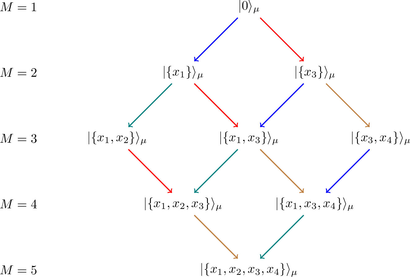
In general, the eigenvalues of the A-operator on the GT descendants have a simple relation to that for the yhw states, \[A_{\mu , \{ u_1, \dots, u_n \} } (x) = A_{\mu} (x) \prod_{m=1}^n \frac{x-u_m+1}{x-u_m} \; .\]
5.2.0.2 Descendants with \(\mathfrak{sl}_2\) symmetry.
In the periodic limit \(\kappa \to1\), the transfer matrix has additional \(\mathfrak{sl}_2\) symmetry. From the Drinfeld polynomial 61 we read off the Clebsch–Gordon decomposition of the Yangian multiplet, viewed as a tensor product of \(\mathfrak{sl}_2\)-multiplets, as shown in Table 1. The two spin-\(1\) representations correspond to the two \(2\)-strings in 61 , while the spin-\(0\) representation corresponds to the contribution of the \(0\)-string. See also Fig. 1. Therefore, there are three \(\mathfrak{sl}_2\)-multiplets: one containing the yhw state (spin \(2\)) and one each whose \(\mathfrak{sl}_2\) highest-weight state has \(K=1\) (spin \(1\)) or \(K=2\) (spin \(0\)) additional Bethe roots.
Solving the TQ relation 49 for the spin-\(1\) \(\mathfrak{sl}_2\) highest-weight state we have \[|\{ -\tfrac{1}{2} \} \rangle_{(3) } \; ,\] and for the spin-\(0\) \(\mathfrak{sl}_2\) highest-weight state we have \[|\{ -\tfrac{1}{2} - \mathrm{i} , -\tfrac{1}{2} + \mathrm{i} \} \rangle_{(3)} \; .\] Taking into account all \(\mathfrak{sl}_2\) descendants we arrive at one spin-\(2\), one spin-\(1\), and one spin-\(0\) \(\mathfrak{sl}_2\) multiplet, \[\begin{gather} \ket{0}_{(3) } \, , \qquad\mathbf{S}^- \, \ket{0}_{(3) } \, , \qquad ( \mathbf{S}^-)^2 \, \ket{0}_{(3) } \, ,\qquad ( \mathbf{S}^-)^3 \, \ket{0}_{(3) }\, ,\qquad ( \mathbf{S}^- )^4\, \ket{0}_{(3) } \, ; \\ |\{ -\tfrac{1}{2} \} \rangle_{(3)} \, , \qquad \mathbf{S}^- \, |\{ -\tfrac{1}{2} \} \rangle_{(3) } \, , \quad ( \mathbf{S}^-)^2 \, |\{ -\tfrac{1}{2} \} \rangle_{(3)} \, ; \quad \\ |\{ -\tfrac{1}{2} - \mathrm{i} , -\tfrac{1}{2} + \mathrm{i} \} \rangle_{(3) } \; . \quad \end{gather}\] This structure of the Yangian multiplet is analogous to that of the usual Heisenberg xxx spin chain. A Hasse diagram for this Yangian-descendant tower with \(\kappa=1\) is shown in Fig. 3. The descendant structure for the whole Hilbert space is as shown in Fig. 1.
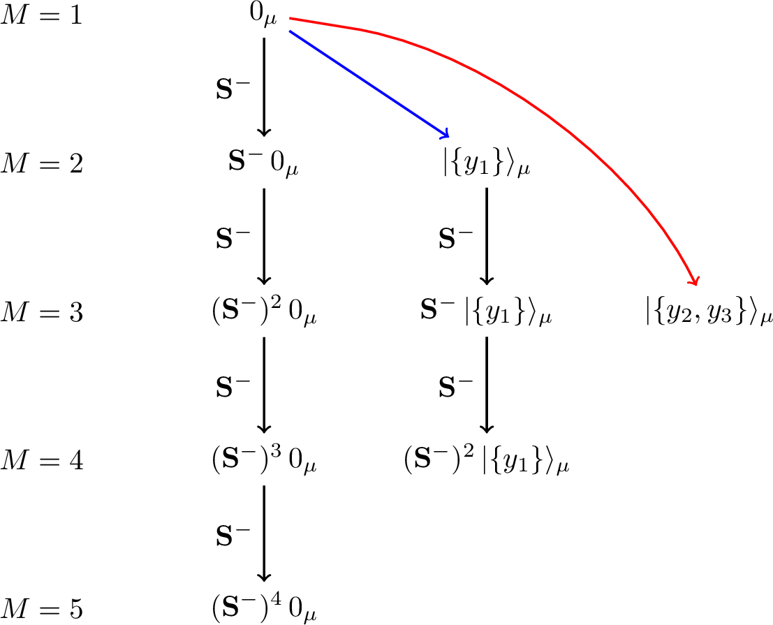
5.2.0.3 Descendants at generic twist.
In this subsection, we present the numerical solutions of the Yangian descendants of the yhw state \(|0\rangle_{(3)}\) with a generic twist, which we take to be \(\kappa = \frac{1}{\sqrt{2}}\) for definiteness.
For Yangian descendants with \(K=1\) additional magnon, we solve the effective \(TQ\)-relation 49 to find two physical solutions, \[\ket{ \{ \tfrac{5+4\sqrt{3}}{2} \} }_{(3) } \; , \quad \ket{ \{ \tfrac{5-4\sqrt{3}}{2} \} }_{(3) } \; .\] In the absence of closed-form Bethe roots, we present the numerical solutions to six digits in the following. Since all non-real Bethe roots come in complex conjugate pairs (\(\kappa>0\)), we use the shorthand \(u\pm v\,\mathrm{i}\) to mean \(u+ v\,\mathrm{i},u- v\,\mathrm{i}\). For Bethe vectors with \(K=2\) additional magnons we find three physical solutions, \[\ket{ \{ 4.35245 \pm 2.23356 \, \mathrm{i}\} }_{(3) } \; , \quad \ket{ \{ -1.55338 \pm 0.519379 \, \mathrm{i}\} }_{(3)} \; , \quad \ket{ \{ -0.698802, 4.10066\} }_{(3)} \; . \label{eq:generickappaM3}\tag{62}\] For \(K=3\) we find two physical solutions, \[\ket{ \{ 3.81572 , 2.07419 \pm 2.98985 \, \mathrm{i}\} }_{(3) } \; , \quad \ket{ \{3.34600 , -1.15505 \pm 0.908272 \, \mathrm{i}\} }_{(3) } \; .\] Finally, for Yangian descendants with \(K=4\) additional magnons, there is only one physical solution, that gives the Yangian lowest-weight state \[\begin{align} \ket{ \{ -0.61811 \pm 2.84188 \, \mathrm{i}, 2.61811 \pm 0.812557 \, \mathrm{i}\} }_{( 3 ) } \propto \prod_{n=1}^6 \! \sigma^x_n \; \ket{ 0 }_{(3) } \; . \end{align}\]
This illustrates that for a generic twist \(\kappa\), the Yangian descendants associated with the twisted transfer matrix \(\mathbf{T}(x;\kappa)\) also provide the correct number of states in the corresponding Yangian multiplet. This time, the Bethe roots of the different Yangian descendants are unrelated, unlike for the special cases \(\kappa\to\infty\) and \(\kappa=1\). Just like for (e.g.twisted xxx, or xxz) Heisenberg chains without \(\mathfrak{su}_2\) symmetry, there is no extra structure in the Yangian descendant tower.
5.2.0.4 Comparison.
For a fixed magnon number \(M\), the descendant states for different \(\kappa\) span the same Hilbert space. Different choices of \(\kappa\) imply different choices of the basis states. For instance, the descendant states with \(M=3\) in 62 span the same Hilbert space as \(|\{x_1, x_2\} \rangle_\mu , |\{x_1, x_3\} \rangle_\mu , |\{x_3, x_4\} \rangle_\mu\) in Fig. 2 span in the limit \(\kappa \to \infty\), and as \((\mathbf{S}^-)^2 |0\rangle_\mu , \mathbf{S}^- |\{y_1\}\rangle_\mu , |\{y_1, y_2\}\rangle_\mu\) in Fig. 3 span when \(\kappa = 1\). These form eigenbases for different extra Heisenberg-style symmetries 4 or 5 , depending on the twist, but are all valid eigenbases for the HS hamiltonian 3 .
6 Conclusion and outlook↩︎
This work provides a detailed and systematic construction of Yangian descendant states for the Haldane–Shastry (HS) chain capitalising on [12]. Since each HS eigenspace can be separately viewed as an ‘effective’ inhomogeneous Heisenberg xxx chain, we use an ‘internal Bethe ansatz’ following [12] by formulating these descendant states as eigenstates of the twisted transfer matrix \(\mathbf{T}(x; \kappa)\) with twist \(\kappa>0\) to ensure hermiticity. Starting from the explicitly known yhw state for a given motif, we derive the bae and TQ-relations for the Bethe roots of its Yangian descendants at given \(\kappa\). With the help of the algebraic Bethe ansatz (aba), the eigenvalues and eigenvectors of the transfer matrix are obtained. The quantum operators require one to go through the spin-CS system and freezing, cf.the end of Sec. 3, meaning that the construction of the explicit Bethe vectors requires some effort. Nevertheless, the aba description enables us to compute their norms and overlaps, yielding compact determinant formulae in terms of the Bethe roots. In the extreme cases \(\kappa\to\infty\) and \(\kappa\to 0\) (the Gelfand–Tsetlin limits), the associated \(TQ\)-relation simplifies considerably and becomes explicitly solvable.
Our results establish a foundation for computing a wide range of physical observables. An immediate and important goal is the analytical study of quantum quench dynamics. In integrable spin chains with nearest-neighbour interaction, such dynamics for integrable initial states [43]–[47], including the Néel state and integrable matrix-product states, have been central to the understanding of non-equilibrium behaviour [43], [48]. Extending similar analytical approaches to long-range interacting systems is highly desirable, particularly given the experimental relevance of such models in platforms such as ion traps. In this context, exact overlap formulas between eigenstates (typically expressed as Bethe states) and integrable boundary states serve as essential inputs. Systematic studies of integrable boundary states as well as their overlaps with energy eigenstates are still lacking for long-range spin chains. The present work constitutes a crucial step toward this direction.
Another interesting direction is the investigation of physical properties at finite temperature. While the thermodynamics of the HS chain has been explored from several perspectives, first via the free-spinon-gas picture [8] and later through more conventional thermodynamic approaches [25], the relationship between these descriptions has recently been revisited in [49]. Moreover, hydrodynamic methods have been applied to examine transport properties in this model [49]. These studies collectively highlight the analytical tractability of the HS chain, for which many physical quantities admit closed-form expressions. A key open problem in this area is the microscopic derivation of the Boltzmann equation system; addressing it will require a deeper understanding of the Hilbert-space structure and descendant states studied here. Although ground-state correlation functions [49]–[52] have been widely examined, finite-temperature correlations remain largely unexplored. Our results also provide a useful basis for advancing research in this direction.
Acknowledgement↩︎
We are indebted to Jean-Sébastien Caux for collaboration in the early stages of this work and for numerous discussions throughout the course of this work. The work of Y.M. was supported by the World Premier International Research Center Initiative (WPI), MEXT, Japan and the UTokyo Global Activity Support Program for Young Researchers. Y.M. is grateful for the hospitality of Rudolf Peierls Centre for Theoretical Physics and St. John’s College at University of Oxford. Y.M. thanks Jiakang Bao, Henry Liu and Masahito Yamazaki for useful discussions on the Yangian. The work of Y.J. is supported by National Natural Science Foundation of China through Grant No.12575073. Y.M. used ChatGPT 5.5 to help read [11]; we acknowledge the use of ChatGPT 5.5 to assist with proofreading the manuscript. The authors of this paper are ordered alphabetically.
7 Yangian relations of quantum operators↩︎
In this appendix, for easy reference we collect some of the well-known non-trivial algebraic relations of quantum operators \(\mathbf{A}(x)\), \(\mathbf{B}(x)\), \(\mathbf{C}(x)\) and \(\mathbf{D}(x)\) contained in the RTT relation 30 . These are useful when deriving the bae (or \(TQ\)-relation) as well as the norm and overlap formulae. The relations read \[\left[ \mathbf{A}(x) , \mathbf{A}(y) \right] = \left[ \mathbf{B}(x) , \mathbf{B}(y) \right] = \left[ \mathbf{C}(x) , \mathbf{C}(y) \right] = \left[ \mathbf{D}(x) , \mathbf{D}(y) \right] = 0 \, ,\] \[\begin{align} & \left[ \mathbf{A}(x) , \mathbf{D}(y) \right] = \frac{1}{x-y} \, \bigl( \mathbf{C}(y) \, \mathbf{B}(x) - \mathbf{C}(x) \, \mathbf{B}(y) \bigr) \; , \\ & \left[ \mathbf{D}(x) , \mathbf{A}(y) \right] = \frac{1}{x-y} \, \bigl( \mathbf{B}(y) \, \mathbf{C}(x) - \mathbf{B}(x) \, \mathbf{C}(y) \bigr) \; , \\ & \left[ \mathbf{C}(x) , \mathbf{B}(y) \right] = \frac{1}{x-y} \, \bigl( \mathbf{A}(y) \, \mathbf{D}(x) - \mathbf{A}(x) \, \mathbf{D}(y) \bigr) \; , \\ & \left[ \mathbf{B}(x) , \mathbf{C}(y) \right] = \frac{1}{x-y} \, \bigl( \mathbf{D}(y) \, \mathbf{A}(x) - \mathbf{D}(x) \, \mathbf{A}(y) \bigr) \; , \end{align}\] \[\begin{align} & \mathbf{A}(y) \, \mathbf{B} (x) = \frac{x-y}{x-y+1} \, \mathbf{B} (x) \, \mathbf{A} (y) + \frac{1}{y-x} \, \mathbf{B} (y) \, \mathbf{A} (x) \; , \\ & \mathbf{B}(y) \, \mathbf{A} (x) = \frac{x-y}{x-y+1} \, \mathbf{A} (x) \, \mathbf{B} (y) + \frac{1}{y-x} \, \mathbf{A} (y) \, \mathbf{B} (x) \; , \\ & \mathbf{D}(y) \, \mathbf{C} (x) = \frac{x-y}{x-y+1} \, \mathbf{C} (x) \, \mathbf{D} (y) + \frac{1}{y-x} \, \mathbf{C} (y) \, \mathbf{D} (x) \; , \\ & \mathbf{C}(y) \, \mathbf{D} (x) = \frac{x-y}{x-y+1} \, \mathbf{D} (x) \, \mathbf{C} (y) + \frac{1}{y-x} \, \mathbf{D} (y) \, \mathbf{C} (x) \; , \end{align}\] \[\begin{align} & \mathbf{A}(x) \, \mathbf{C} (y) = \frac{x-y}{x-y+1} \, \mathbf{C} (y) \, \mathbf{A} (x) + \frac{1}{y-x} \, \mathbf{C} (x) \, \mathbf{A} (y) \; , \\ & \mathbf{C}(x) \, \mathbf{A} (y) = \frac{x-y}{x-y+1} \, \mathbf{A} (y) \, \mathbf{C} (x) + \frac{1}{y-x} \, \mathbf{A} (x) \, \mathbf{C} (y) \; , \\ & \mathbf{B}(x) \, \mathbf{D} (y) = \frac{x-y}{x-y+1} \, \mathbf{D} (y) \, \mathbf{B} (x) + \frac{1}{y-x} \, \mathbf{D} (x) \, \mathbf{B} (y) \; , \\ & \mathbf{D}(x) \, \mathbf{B} (y) = \frac{x-y}{x-y+1} \, \mathbf{B} (y) \, \mathbf{D} (x) + \frac{1}{y-x} \, \mathbf{B} (x) \, \mathbf{D} (y) \; . \end{align}\]
8 Inhomogeneous Heisenberg xxx chain↩︎
In this appendix, we consider an inhomogeneous Heisenberg xxx chain with linearly increasing inhomogeneities. We will show that it contains a similar Yangian descendant structure as the HS chain.
We define the inhomogeneous monodromy and transfer matrices as \[\begin{align} & \mathbf{M}_{a}^{\rm inh} (x) = \mathbf{R}_{a1}\Bigl(x-\xi_1 -\tfrac{1}{2}\Bigr) \cdots \mathbf{R}_{aN} \Bigl(x-\xi_N - \tfrac{1}{2}\Bigr) = \begin{pmatrix} \mathbf{A}^{\rm inh}(x) & \mathbf{B}^{\rm inh}(x) \\ \mathbf{C}^{\rm inh}(x) & \mathbf{D}^{\rm inh}(x) \end{pmatrix}_{\!a} \; , \\ & \mathbf{T}^{\rm inh} (x ; \kappa) = \kappa \,\mathbf{A}^{\rm inh} (x) + \kappa^{-1} \, \mathbf{D}^{\rm inh} (x) \; . \end{align}\] Following §4.3.2 of [12], we choose the following (maximally non-generic) inhomogeneities \[\xi = \{ -\tfrac{N-1}{2} , -\tfrac{N-3}{2} , \cdots , \tfrac{N-1}{2} \} \; ,\] such that all neighbouring inhomogeneities differ by \(\xi_n - \xi_{n-1} = 1\), meaning that we encounter (antisymmetric) fusion at each pair of sites, see e.g.§2.2.4 in [12]. In particular, one important observation is that given a sequence of integers \(\mu = \{ \mu_1, \dots , \mu_M\}\) obeying the motif conditions 6 , the state \[\label{eq:inh95mu} \ket{\mu}^{\rm inh} \mathrel{\vcenter{:}}= \prod_{m=1}^M \! \mathbf{B} \Bigl(\mu_m -\tfrac{N+1}{2}\Bigr) \, \ket{\uparrow\cdots\uparrow} \propto \prod_{m=1}^M \! \bigl( \sigma_{\mu_m + 1}^- - \sigma_{\mu_m}^- \bigr) \, \ket{\uparrow\cdots\uparrow} \,\tag{63}\] has singlets \(\ket{\uparrow\downarrow}-\ket{\downarrow\uparrow}\) at pairs of neighbouring sites \((\mu_m,\mu_m+1)\) indicated by the motif. Moreover, the state \(\ket{\mu}^\mathrm{inh}\) has yhw, \[\begin{pmatrix} \mathbf{A}^\mathrm{inh}(x) & \mathbf{B}^\mathrm{inh}(x) \\ \mathbf{C}^\mathrm{inh}(x) & \mathbf{D}^\mathrm{inh}(x) \end{pmatrix}_{\!a} \ket{\mu}^\mathrm{inh} = \begin{pmatrix} A_\mu(x) \, \ket{\mu}^\mathrm{inh} & \ast \\ 0 & D_\mu(x) \, \ket{\mu}^\mathrm{inh} \end{pmatrix}_{\!a} \, ,\] with the same eigenvalues 39 –40 as for the yhw state \(\ket{0}_\mu\) in the HS chain. We refer the readers to [12] for a more detailed explanation.
8.1 The Q-system↩︎
Solving the bae or \(TQ\)-relation 49 for the inhomogeneous Heisenberg xxx chain leads to both physical and unphysical solutions. To get a (complete) set of Bethe roots of inhomogeneous xxx chain that precisely correspond to the physical states, one can solve the rational Q-system. We briefly review the Q-system in this appendix. For more details and examples we refer to [53]–[55].

For the (inhomogeneous) bae with length \(L\) and \(M\) magnons, the Q-system is associated to a two-row Young diagram \((L-M,M)\), illustrated in Fig. 4. We use the French notation for the Young diagram, i.e.the longer row is at the bottom. At each node of the Young diagram we define a function of the spectral parameter \(u\), denoted by \(Q_{a,n}(u)\) where \((a,n)\) is the lattice coordinate of the node on the Young diagram, cf. Fig. 4. The Q-functions are not independent: the Q-functions at the four corners of each box are related by the QQ-relation \[\label{eq:rationalQsys} \begin{align} Q_{0,n} \, Q_{1,n-1} & = \kappa \, Q_{0,n-1}^+ \, Q_{1,n}^- - \kappa^{-1} \, Q_{0,n-1}^- \, Q_{1,n}^+ \;, \\ Q_{1,n} & = Q_{1,n-1}^+ - Q_{1,n-1}^- \; , \end{align} \qquad n \geqslant 1 \;,\tag{64}\] where \(\kappa\) is the twist in the transfer matrix and we have fixed \(Q_{2,n}=1\) as part of the boundary conditions. We use the notation \(f^{\pm}(x) \mathrel{\vcenter{:}}= f(x \pm \frac{1}{2})\) to denote the shift of argument of a function. The Q-functions at the left boundary are also completely or partly fixed. In particular, we define \[Q_{0,0} (x) = \prod_{n=1}^N (x- \xi_n) = \prod_{n=1}^N \Bigl( x + \tfrac{N+1}{2}-n \Bigr) \; ,\] which is completely fixed.
The Baxter’s Q-function \(Q_{1,0}\) is fixed to take the following form \[\begin{align} Q_{1,0} (x) = Q_{\mu,\boldsymbol{{u}}} \Bigl(x - \tfrac{1}{2} \Bigr) & = \prod_{m=1}^M \! \Bigl( x- \tfrac{N+1-2\,\mu_m}{2} - \tfrac{1}{2} \Bigr) \prod_{k=1}^{K} \! \Bigl( x- u_k - \tfrac{1}{2} \Bigr) \\ & = \prod_{m=1}^M \! \Bigl( x- \tfrac{N+1-2\,\mu_m}{2} - \tfrac{1}{2} \Bigr) \left(x^{K} + \sum_{k=0}^{K-1}c_k \, x^k \right) \; , \end{align}\] for Yangian pseudovacuum \(|\mu \rangle^{\rm inh}\). Note that \(Q_{1,0}(x)\) is only partly fixed because we still need to find the Bethe roots \(\{u_k\}_{k=1}^{K}\). We further impose the analytic condition that all the Q-functions on the Young diagrams are polynomials in \(x\). This leads to a set of equations for the coefficients \(c_0,\dots,c_{K-1}\) called zero-remainder conditions. Solving these equations for the coefficients \(c_k\) gives the polynomial \(Q_{1,0}(x)\) and thus its zeroes, i.e.the Bethe roots.
By solving the rational Q-system 64 , we obtain precisely all physical solutions to the inhomogeneous Heisenberg xxx chain.
The solutions to the Q-system are in one-to-one correspondence with the HS eigenstates. The Yangian descendants for the HS chain can be obtained by acting with \(\prod_{k=1}^K \mathbf{B}(u_k)\) on the corresponding yhw state \(\ket{0}_\mu\). For a fixed value of the twist \(\kappa\), the \(TQ\)-relations 49 of the HS chain are equivalent to the QQ-relations 64 with \(n=1\).
However, an important difference between the inhomogeneous xxx chain and HS chain is the form of the yhw states. For the inhomogeneous xxx chain, these consists of \(\uparrow\)s combined with singlets realising the motif in real space, and can be obtained via acting with the B-operator as in 63 . In contrast, the yhw states of the HS chain are given in terms of Jack polynomials, and cannot be obtained simply by acting with B-operators on the ferromagnetic vacuum \(\ket{\uparrow \cdots \uparrow}\), and the motifs rather manifest themselves in momentum (or spectral) space, see Sec. 2.2. Nevertheless, the eigenvalues of the A- and D-operators on the yhw states for the two spin chains coincide for a given motif \(\mu\).
References↩︎
The dressed scattering phase for spinons, i.e.the excitations over the antiferromagnetic ground state, is also momentum-independent [26], indicating the free semionic gas nature of the HS chain [27].↩︎
Note that this notion of ‘\(\ell\)-string’ differs from the concept with the same name in the context of complex Bethe roots and bound states in the Heisenberg chain.↩︎
Compared to [31], we have used the property \(P_{\lambda+1}(z_1,\dots,z_M) = z_1 \cdots z_M \, P_\lambda(z_1,\dots,z_M)\) of Jack polynomials to decrease all parts of the partition by \(1\).↩︎
The values of the inhomogeneities are such that fusion occurs (often), cf. [12], and the Bethe ansatz is complete [34]–[36].↩︎
The sign of the Dunkl operators in 29 depends on the order of the factors of the monodromy matrix and whether one considers the bosonic or fermionic spin-CS system. The monodromy matrix 29 is ordered as in [12], for which the fermionic constraint 25 requires replacing the usual inhomogeneities by \(-d_j\). Ref.[29] uses the opposite monodromy matrix, in which case the signs of the Dunkl operators are opposite: the monodromy matrix \(\mathbf{R}_{aN}(x-d_N-\tfrac{1}{2})\cdots \mathbf{R}_{a1}(x-d_1-\tfrac{1}{2})\) is also compatible with 25 .↩︎
In short, the argument goes as follows. Step [it:HS95wf95from95ev] holds for the yhw states, see 35 –36 . The unevaluated vector can in fact be lifted to an element of the spin-CS Hilbert space. (This is nontrivial.) By completeness, any other vector can be obtained from yhw states using the HS Yangian. But the latter come from spin-CS Yangian operators, which send fermionic spin-CS vectors to fermionic spin-CS vectors. Thus, Step [it:HS95wf95from95ev] holds for any eigenstate.↩︎
This property is more easily proved in the language of spin-CS system, where there exists an inner product (with measure the square of 24 ) on functions of the coordinates such that the Dunkl operators are hermitian. This inner product extends to an inner product on \(\mathbb{C}[z_1^{\pm1} , \dots , z_N^{\pm1}] \otimes (\mathbb{C}^2 )^{\otimes N}\) for which the monodromy matrix \(\widetilde{\mathbf{M}}_a (x)\) is ‘hermitian’ (self-adjoint) [11]. In the freezing limit this implies 44 .↩︎
We remark that the same combinatorial structure appears for the \(q\)-deformed HS chain in the crystal limit \(q \to 0\) [31], where it is realised directly on the lattice: the affine highest-weight vectors become proportional to \(\cket{\mu} = \prod_{n\in \mu} \sigma^-_n \; \ket{\uparrow\cdots\uparrow}\), and descendants correspond to extending domains of \(\downarrow\)s to the right without merging domains.↩︎