Trends, Volatility, Correlations,
and Critical Phenomena in Financial Markets
June 18, 2026
Abstract
We forecast future volatilities and correlations of financial markets based on the current trends in these markets. This complements previous work that models future expected returns by a cubic polynomial of the current trend strength. Empirically, we observe that volatilities and correlations tend to increase day after day in times of strong up- or down-trends. This effect is particularly pronounced in down-trends. It can be accurately quantified by quadratic polynomials of today’s trend strengths, which refine common mean-reversion models of volatilities and correlations. Our results improve the prediction of market risk by accounting for market trends. They also support a recent proposal to model financial markets by a lattice gas near its critical point.
1 Introduction↩︎
Over the past decades, market trends have proven to have a tiny but still statistically significant predictive power for future returns. This effect has been very profitably exploited by the trend-following industry at least since the turtle traders in
the 1980’s [1]. It has also been confirmed in many academic studies, such as [2]–[9]. More recently, it has been shown that the predictive power of market trends is not a new phenomenon but dates back at least a few centuries [10]–[13].
In [10], it has been noted that trends tend to revert once they become too strong, and this has been modeled quantitatively in [14]. In [15], we have independently confirmed these results by carefully
measuring the next-day mean return in a market as a function of its trend strength on a given day. To filter out the statistical noise and get sufficiently precise results, it was crucial to aggregate not only across decades of daily market data for a
broadly diversified set of financial markets, but also across 10 trend horizons ranging from days to years. This aggregation makes sense, because - as is well-known in practice - similar trend-following strategies tend to work over a wide range of time
scales.
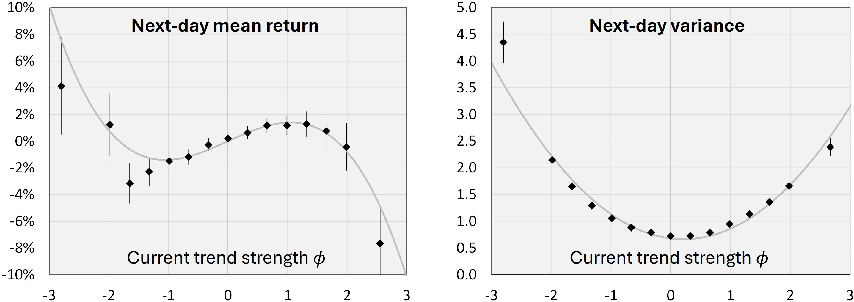
A key finding of [15] is illustrated in fig. 1 (left): trends tend to revert before they become statistically strongly significant. This means
that as soon as a trend has become so obvious that it is clearly visible in a price chart, it is already too late to join it. This is consistent with the hypothesis [16] that any obvious market inefficiency is quickly eliminated by investors. More precisely, for a given market and a given time horizon, we have defined the strength \(\phi\) of a trend as
its \(t\)-statistics. We have found that tomorrow’s return \(r_{t+1}\) (normalized to have variance 1) is modeled well by a cubic polynomial of today’s trend strength \(\phi_t\): \[\begin{align}
r_{t+1}&=&a\;+{b}\cdot \phi_t+{c} \cdot \phi_t^3+\epsilon_{t+1},\label{cubic}\\
\text{with}&&b\;=\;0.013\pm0.004\;,\;\;\;c\;=\;-0.006\pm0.002,\notag
\end{align}\tag{1}\] where the random noise \(\epsilon\) is not required to be identically and independently distributed. Here, \(a\) is a risk premium, which depends on the
asset. However, the kinetic coefficients \(b\) and \(c\) are universal in the sense that they seem to be the same for all assets within the limits of statistical significance. \(b\) is interpreted as the persistence of trends, and \(c\), which is negative, as the strength of trend reversion. Both are statistically highly significant, while quadratic and higher-order
polynomial terms in (1 ) are not or only weakly significant. Model (1 ) is in line with practical experience of the trend-following industry. It has been extended to intraday- and many-year-time scales [10], [13].
In this paper, we empirically analyze the noise \(\epsilon\) in (1 ) in more detail and find that it has a rich and interesting structure. As a simple illustration, fig. 1 (right) plots the
expectation value of tomorrow’s square return \(r_{t+1}^2\) against today’s trend strength. This yields a slightly skewed parabola with only small estimation errors. It shows that the variance of tomorrow’s return is much
higher in times of strong up- or down-trends.
We will quantify and refine this observation by precisely measuring the expected future variance as a function of both today’s trend strength and today’s variance. Similarly, we measure tomorrow’s expected correlation of the returns of different assets as
a function of today’s trend strengths and today’s correlation. We find that the variance and the correlations can be modeled well by second-order polynomials in these explanatory variables.
Our results are based on 33 years of daily futures returns for 24 different markets, diversified across different asset classes (equity indices, interest rates, FX rates and commodities) and across different time zones (Americas, Europe and Asia). These
data, which are marked-to-market daily, are described in more detail in appendix A. Our precise definition of the trend strength and the statistical methodology, including bootstrapping and out-of-sample cross validation, follows that in [15] and is briefly summarized in appendix B.
This paper is organized as follows. Section 2 presents our empirical measurements of the next-day variance. We first perform a nonlinear regression analysis of the variance. The results refine mean-reverting variance models [17], [18] such as the AR(1) variance model or the Heston volatility model [19] by also taking current market trends into account. We then pursue an alternative ansatz, in which we model the log-variance instead of the variance. These results refine mean-reverting
stochastic log-volatility models such as the Hull-White model [20] by including trends.
Section 3 presents our empirical results regarding next-day correlations. In particular, this quantifies the well-known fact that markets are more correlated in times of crises, which are typically accompanied by strong trends. Section 4 measures how the
skewness and kurtosis of the distribution of next-day returns depend on today’s trend strength. While we do not find a highly significant dependence, we show that integrating over the trend strength replicates the overall skewness and kurtosis observed in
financial markets.
Our results allow for a refined prediction of market risk and correlations by also taking current market trends into account. As such, they can contribute to an improvement of market risk management tools, especially for periods of market crises. However,
they are also relevant for the search of a financial market model that can explain all observed stylized facts of finance [21]–[23]. In this context, section 5 shows that our empirical observations are consistent with the recent proposal [24], [25] of modeling financial markets by a lattice gas near its critical point. Section 6 contains a summary and conclusions.
2 Variance↩︎
In this section, we model the future variance of returns as a function of the current trend strength, aggregated across all 24 markets, 10 time scales, and 33 years of data as described in appendix A. We follow the nonlinear regression methodology described in appendix B. A new element is that we must also include the current variance in the regression, as it is an important explanatory variable.
2.1 Visualization of the Data↩︎
We first visualize these data by grouping them into 15 bins \(b_k\) of similar trend strength: \[\phi\in
b_k\;\;\;\text{with}\;\;\;k\in\{-7,+7\},\;\;\;b_k=[\;{k\over3}-{1\over6}\;,\;{k\over3}+{1\over6}\;[\;.\label{buckets}\tag{2}\] I.e., bucket \(b_0\) covers trend strengths from \(-1/6\) to \(+1/6\), \(b_1\) from \(+1/6\) to \(+1/2\), and so on. We extend the outermost
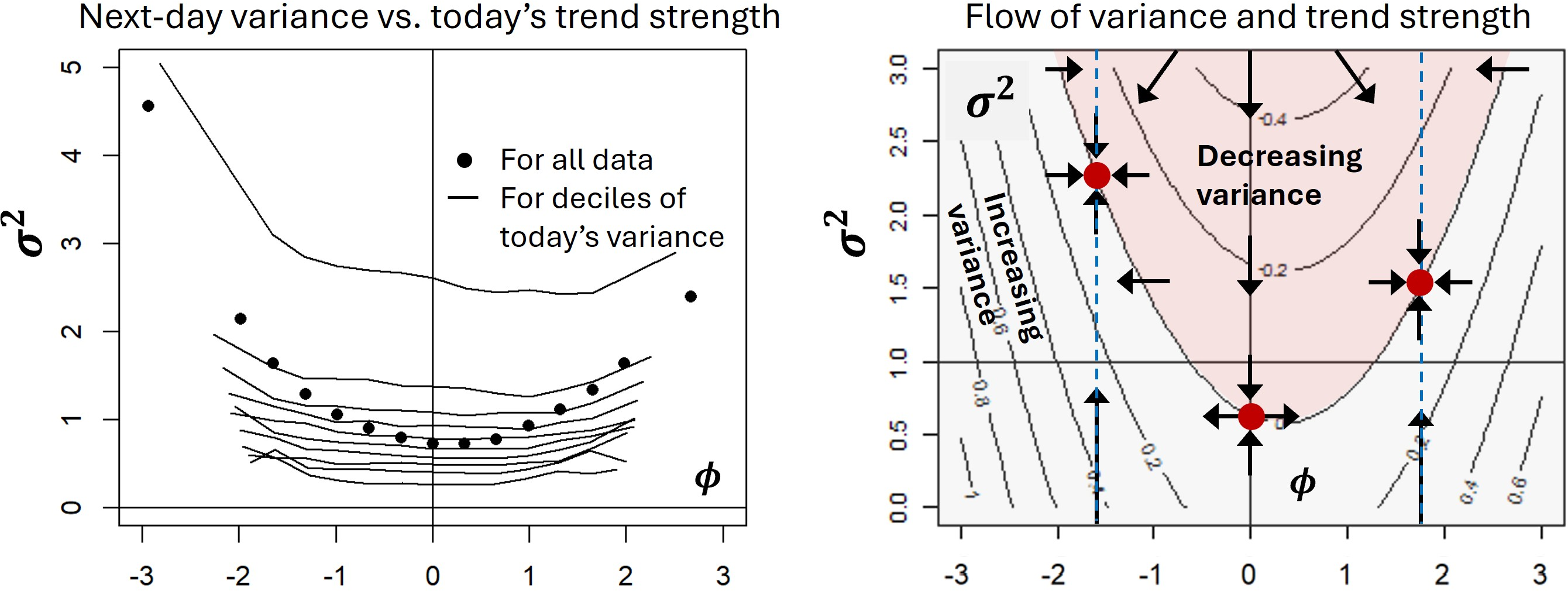
buckets \(b_{\pm7}\) to \(\pm\infty\). We then measure the variance of next-day returns \(r_{t+1}\), given that the trend strength lies in bin \(b_k\) on day \(t\). For daily data, the dots in fig. 1 (right) and in fig. 2 (left) show this variance for each bin as a function of the average trend strength in that bin. The results are
aggregated across the 10 different trend horizons \(T\in\{2,4,8,...,1024\}\) days. The figures suggest to model tomorrow’s variance by an at least second-order polynomial of today’s trend strength. This polynomial appears
to have a negative linear component: the parabola in fig. 2 (left) looks like a skewed "smile".
The variance \(\sigma_t^2\) of financial market returns on day \(t\) is well-known to be auto-correlated and to come in clusters. Therefore, we should also include today’s variance as
another important explanatory variable for tomorrow’s variance. We measure the variance by an exponentially-weighted moving average (EWMA), defined as \[\sigma_{t+1}^2\;=\;(1-\alpha)\sum_{i=0}^\infty \alpha^i\cdot
r_{t+1-i}^2\;=\;\sigma_{t}^2+\alpha (r_{t+1}^2-\sigma_t^2)\;\;\;\text{with}\;\;\;\alpha=1-e^{-1/16}.\] Here, we neglect the tiny mean of \(r_{t+1}\) that we have modeled in (1 ). Fig. 2 (left)
repeats the above analysis for each decile of the past 60-day variance (solid lines). The dependence of tomorrow’s variance on today’s trend strength still looks like a skewed smile, but with much smaller curvature. In addition, there is a dependence on
today’s variance, which grows monotonously with today’s trend strength. Apparently, much of the quadratic dependence of tomorrow’s variance on today’s trend strength is already contained in today’s variance.
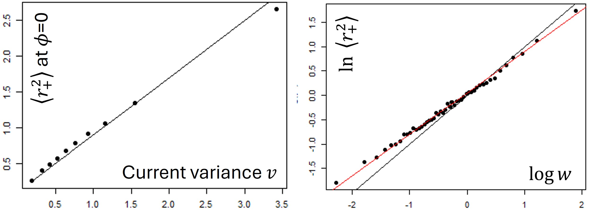
Fig. 3 (left) plots the average of tomorrow’s square return \(\langle r_{t+1}^2\rangle\) (as an estimate of the future variance) against today’s variance \(\sigma_t^2\). At first sight,
\(\langle r_{t+1}^2\rangle\) seems to be an almost linear function of \(\sigma_t^2\). However, a more fine-grained log-log plot (fig. 3, right) suggests that \(\langle r_{t+1}^2\rangle\) could alternatively be modeled as a power \((\sigma_t^2)^\kappa\) with \(\kappa\approx0.8-0.9\). We will try out both models below.
The simple linear model is the subject of subsections 2.2 and 2.3, while the alternative power-law model is discussed in subsection 2.4.
Fig. 2 (right) shows a contour plot of the change of the variance \(\sim \langle r_{t+1}^2-\sigma_t^2\rangle\) as a function of both the trend strength (horizontal axis) and today’s variance (vertical axis). Arrows indicate
the changes of the variance and the trend strength; it follows from (1 ) that the trend strength is driven to \(\phi=\sqrt{b/c}\approx\pm1.5\), where the expected next-day return minus the long-term
risk premium is zero. This yields a fixed line in the flow diagram of fig. 3 (right) with 2 stable and 1 unstable fixed points. In times of strong trends, the variance tends to increase day after day towards the fixed line. This explains why the variance
is high after strong trends have been developing: it is natural to identify the fixed line in fig. 2 (right) with the parabola in fig 2 (left).
2.2 Regression Analysis↩︎
We now quantify these qualitative observations. Figure 2 (left) suggests to model the square of tomorrow’s return by a linear function of today’s variance and a quadratic polynomial of today’s trend strength: \[r_{t+1}^2=a+d\sigma_t^2+e\phi_t+f\phi_t^2+\epsilon_{t+1}^2, \label{volatrend}\tag{3}\] where \(\epsilon\) is the noise. We have also tried out other functions of the trend strength, such
as trigonometric functions, \(n\)-th roots, etc., but the second order polynomial regression has yielded the best adjusted R-squared, as measured empirically by out-of-sample cross validation as described in appendix
B.
| Variance Regression | Trends and variance | Only trends | Only variance | |||
|---|---|---|---|---|---|---|
| Coefficient | Value | t-stat. | Value | t-stat. | Value | t-stat. |
| \(a\) | \(+0.131\) | 3.2 | \(+0.675\) | 58.3 | \(+0.166\) | 3.2 |
| \(d\) | \(+0.793\) | 16.1 | - | - | \(+0.833\) | 15.3 |
| \(e\) | \(-0.061\) | 8.0 | \(-0.148\) | 11.5 | ||
| \(f\) | \(+0.094\) | 11.7 | \(+0.396\) | 34.8 | ||
| \(R^2\) single/aggr. | 0.120 | 0.125 | 0.029 | 0.039 | 0.118 | - |
| \(R^2_{adj}\) single/aggr. | 0.118 | 0.122 | 0.027 | 0.034 | 0.116 | - |
Table 1 shows the regression results, aggregated across trend horizons \(T\) ranging from 2 days to 4 years. We observe that the variance is the most significant factor, with \(d-1\approx-0.2\) measuring how strongly the variance tends to revert to its equilibrium value. However, the linear (\(e\)) and quadratic (\(f\)) dependencies on
the trend strength are also highly significant. \(f\) is positive, which explains why the variance keeps growing during strong trends. \(e\) is negative, which reflects the asymmetry of
fig. 2 (left). This is in line with the so-called "leverage effect" in equity markets, given that trends measure cumulative recent returns: strong negative returns tend to trigger a subsequent rise of volatility.
For comparison, table 1 also shows the regression results with only trends or only variance as explanatory factors. We see that all three factors are needed to maximize the out-of-sample \(R^2\). The \(R^2\) is reported in table 1 both for using only a single trend horizon ("single"), and for using all 10 trend horizons simultaneously to predict the variance ("aggr."). In the latter case, the parameters \(d, e\) in (3 ) multiply the sums of 10 \(\phi_t\) and \(\phi_t^2\) terms, respectively. Although this slightly improves the
out-of-sample R-squared, for simplicity we will focus on the case "single" in the following.
Let us interpret these results. Simple mean-reverting variance models (see, e.g., [17], [18]) predict the
next-day variance from today’s variance \(\sigma^2\) and the long-term variance \(\sigma_0^2\) as \[\sigma^2_{t+1}=\lambda\sigma_0^2+(1-\lambda)\sigma_t^2,\] such that the variance reverts to its equilibrium value \(\sigma_0^2\) within a time span of order \(1/\lambda\) trading days. In our case, \(\sigma_0^2=1\). The results without trend terms in table 1 imply that \(\lambda=0.17\). Ansatz (3 ) refines such models by taking not only the current variance, but also the current trend strength \(\phi_t\) into account. This can be generalized to refine models such as the Heston volatility
model [19]. Our empirical results should also help to develop GARCH models [26] that account for trends in a time-asymmetric way and thereby include the leverage effect, as suggested in [27]. This
should have important applications in financial market risk management, as it allows for a better prediction of market risk.
2.3 Refinements by Time Horizon and Asset Class↩︎
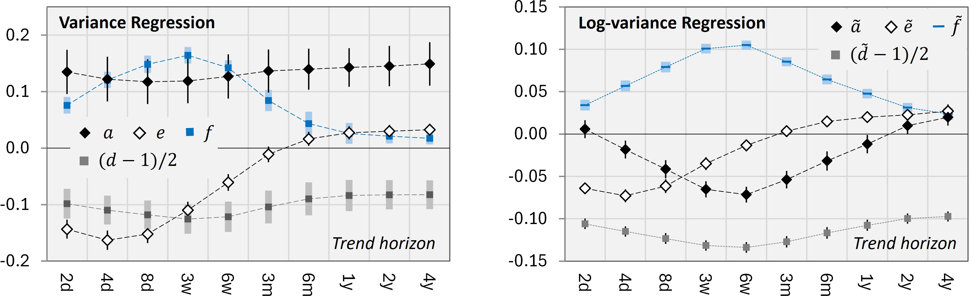
The regression results of table 1 are aggregated over trend time horizons \(T=2^k\) days with \(k\in\{1, ..., 10\}.\) We have repeated this analysis for each \(k\) individually (fig. 4, left). One observes that the coefficients related to the trend strength (\(e,f\)) become insignificant for \(T\ge2^7\) days \(\approx 6\) months. Thus, only trends with horizons up to 3 months have significant predictive power for the future variance. The linear term, which is responsible for the asymmetry of fig. 2 (left), mostly stems from even
shorter trend horizons up to a few weeks.
| Variance | Equities | Interest rates | Currencies | Commodities | ||||
|---|---|---|---|---|---|---|---|---|
| Coefficient | Value | t-stat | Value | t-stat | Value | t-stat | Value | t-stat |
| \(a\) | \(+0.10\) | 2.5 | \(+0.16\) | 4.9 | \(+0.16\) | 3.1 | \(+0.14\) | 1.3 |
| \(d\) | \(+0.82\) | 14.9 | \(+0.76\) | 19.3 | \(+0.76\) | 13.4 | \(+0.79\) | 5.8 |
| \(e\) | \(-0.17\) | 10.9 | \(-0.03\) | 2.8 | \(-0.03\) | 1.9 | \(-0.03\) | 1.5 |
| \(f\) | \(+0.13\) | 6.6 | \(+0.08\) | 7.8 | \(+0.08\) | 6.6 | \(+0.09\) | 3.3 |
| \(R^2,R^2_{adj}\) | 0.166, 0.158 | 0.100, 0.099 | 0.092, 0.086 | 0.101, 0.099 | ||||
To check if the results depend on the asset class, we have repeated the analysis separately for equity indices, interest rates, currencies and commodities. The results are shown in table 2. One observes that the results for interest rates, currencies, and commodities are universal within estimation errors (the errors can be reproduced by dividing the values by the \(t\)-statistics). However, equities seem to have a much stronger linear dependence on the trend strength than the other asset classes. In fact, each of our six equity indices turns out to yield the same high value of \(e\) within the limits of statistical significance. This confirms that the leverage effect is mostly an equity phenomenon.
| Period | a | \(t_a\) | d | \(t_d\) | e | \(t_e\) | f | \(t_f\) | \(R^2\) | \(R^2_{adj}\) |
|---|---|---|---|---|---|---|---|---|---|---|
| 1 day | 0.13 | 3.2 | 0.79 | 16.1 | \(-0.06\) | 8.0 | 0.09 | 11.7 | 0.120 | 0.118 |
| 2 days | 0.13 | 3.8 | 0.79 | 15.1 | \(-0.07\) | 6.3 | 0.10 | 8.5 | 0.185 | 0.183 |
| 1 week | 0.17 | 4.4 | 0.74 | 12.1 | \(-0.07\) | 4.5 | 0.11 | 8.1 | 0.272 | 0.270 |
| 2 weeks | 0.23 | 3.6 | 0.67 | 8.3 | \(-0.06\) | 3.0 | 0.12 | 8.0 | 0.336 | 0.330 |
| 1 month | 0.29 | 4.2 | 0.61 | 6.7 | \(-0.05\) | 1.9 | 0.12 | 5.1 | 0.360 | 0.354 |
| 3 months | 0.34 | 4.2 | 0.60 | 5.6 | \(-0.00\) | 0.04 | 0.08 | 3.6 | 0.420 | 0.380 |
Finally, we have repeated the analysis to predict the variance not just for the next day, but for the next 2 days, 1 week, 2 weeks, 1 month and 3 months. This is relevant for longer-term investors who trade and risk-manage their assets on a weekly, monthly, or quarterly rather than a daily basis. The results are shown in table 3. Since the variance now reverts to its long-term mean over \(n\) consecutive days, we expect the weight \(a\) of the long-term variance to increase with \(n\), while \(d\) decreases. This is indeed what we observe. The linear and quadratic trend-dependence \(e\) and \(f\) is quite stable, but starts to become less significant for \(T>3\) months. This is in line with our observation from fig. 4 (left) that only shorter-term trends significantly influence the future variance.
2.4 Log Variance Model↩︎
In this section, we explore an alternative model of the future variance that is more natural from the viewpoint of stochastic log-volatility models, as opposed to stochastic volatility models. We have seen in fig. 3 (right) that, in the absence
of trends, the next-day square-return can be modeled slightly more accurately as \[\ln\langle r_{t+1}^2\rangle\;\approx\;\tilde{d}\cdot \ln \sigma_t^2\;\;\;\text{with}\;\;\;\tilde{d}\;\approx\;0.8.\] We therefore set up
another regression for the change of the log variance, \[\ln\langle r_{t+1}^2\rangle-\ln\langle r_{t}^2\rangle\;\approx\;{\langle r_{t+1}^2\rangle-\langle r_{t}^2\rangle\over\langle r_{t}^2\rangle}={\langle
r_{t+1}^2\rangle\over\sigma_{t}^2}-1.\] Including powers of the current trend strength \(\phi_t\) as explanatory factors as before yields the alternative regression ansatz \[{\langle r_{t+1}^2\rangle\over \sigma_t^2}\sim 1+\tilde{a}+(\tilde{d}-1)\cdot\ln\sigma_t^2
+\tilde{e}\phi_t+\tilde{f}\phi_t^2+\text{noise}.
\label{logvar}\tag{4}\] Table 4 show the corresponding regression results with and without the trend terms. As expected, \(\tilde{d}\) is indeed of order 0.8 in both cases. \(\tilde{d}-1\) measures the tendency of the log-variance to revert. This quantifies the nonlinear scaling \(\langle r_+^2\rangle\sim d\cdot v^{0.8}\) in fig. 3 (right) more precisely.
Regarding the trend terms, both \(\tilde{e}\) and \(\tilde{f}\) are statistically highly significant. As in the linear model, \(\tilde{e}\) is negative,
reflecting the leverage effect. \(\tilde{f}\) is again positive, reflecting the fact that the variance grows in times of strong trends.
Fig. 4 (right) shows the same coefficients for each trend horizon. As for the variance in fig. 4 (left), only shorter-term trends are helpful in predicting the log-variance.
| Table | Trends and variance | Only variance | ||
|---|---|---|---|---|
| Coeff. | Value | t-stat. | Value | t-stat. |
| \(\tilde a\) | \(-0.024\) | 2.5 | \(+0.043\) | 3.5 |
| \(\tilde d\) | \(+0.760\) | 71.8 | \(+0.815\) | 79.7 |
| \(\tilde e\) | \(-0.022\) | 4.5 | ||
| \(\tilde f\) | \(+0.066\) | 20.1 | ||
| \(R^2, R^2_{adj}\) | 0.0054, 0.0053 | 0.0039, 0.0038 | ||
Modeling the log-variance or log-volatility is natural in stochastic log-volatility models such as the Hull-White stochastic volatility model [20], the SABR model [28], or the more refined multifractal random walk [29]. There, the volatility \(\sigma^2(t)=e^{\xi(t)}\) is an independent random variable, in addition to the asset price \(\pi(t)\). \(\sigma(t)\) multiplies the original returns \(\dot{\hat{\pi}}(t)\) (the changes of the normalized asset price), whose variance is assumed to be constant. In the simplest cases, its logarithm \(\xi(t)\) is a free or mean-reverting random walk: \[\dot{\pi}(t)= \dot{\hat{\pi}}(t)\cdot e^{\xi(t)/2}, \;\;\;{\dot{\xi}}=a+(\tilde{d}-1)\xi+\eta,\] where \(\eta\) is Gaussian noise. This simple model, in which \(\xi\) and \(\hat{\pi}\) are independent, cannot explain the observed leverage effect, according to which negative market returns increase the future variance. Our ansatz (4 ) generalizes this simple model by including the trend strength. It can thereby also replicate the leverage effect. In section 5, we show that it naturally arises in a random network model of financial markets near its critical point.
3 Correlations↩︎

In the previous section, we have measured the next day’s variance of an asset as a function of the strength of the current price trend of that asset. In this section, we measure the correlation of two assets as a function of their respective trend strengths. A complication is that our daily futures prices are recorded at different closing hours, depending on the exchange on which they are traded. This significantly underestimates correlations across regions (US, Europe, Asia). We cannot retroactively synchronize the data, as we have no 33-year history of intraday prices. To at least reduce this error, we therefore build 1560 blocks of weekly asset returns (5 business days) from the daily returns, and work with the correlations of those weekly returns in this section.
3.1 Data Visualization↩︎
We again first take a qualitative look at the data. For this first look, we focus on a trend horizon of \(T=2^6=64\) days; we will later discuss how the results depend on the horizon. There are \(24\cdot23/2=276\) pairs of our \(24\) assets. For each asset pair and each of the \(1560\) weeks in our data set, we measure the pair of trend strengths (\(\phi_t,\psi_t\)) at the end of the week, as well as the pair of next-week returns \((r_{t+1},s_{t+1})\). We group each of the two trend strengths into 6 buckets corresponding to trend strengths
(\(\phi<-2, -2\le\phi<\-1, ..., 2<\phi\)). This leaves us with \(36\) bucket pairs, each of which covers, on average, each of the 276 asset pairs on \(1560/36\approx 43\) weeks. For each bucket and each asset pair, we measure the deviation of the correlation \(\rho_{t+1}\) of the next-week returns from their long-term correlation \(\rho_0\) (which is independent of the trend strength). We then average this deviation over all asset pairs.
The heat map in fig. 5 shows the resulting average deviation of the correlation from its long-term average as a function of the two trend strengths. We observe a saddle-like pattern: the correlation is about 0.15 higher than the long-term correlation, when
both trends are strong and point down. It is also higher, although to a lesser extent, when both trends point up. When one asset is in a strong up-trend and the other is in a strong down-trend, the correlation is about 0.2 lower. It is close to the
long-term correlation in the absence of significant trends. We find similar patterns for other trend horizons (see below).
These observations have a natural interpretation: our data set includes various market crises. As commonly perceived by investors, assets are more strongly correlated in crises: all equities and other risky assets tend to "go down together", while bonds
and safe-haven assets such as gold (which are negatively correlated with equities at least in crises) sharply appreciate. The corners of fig. 5 apparently reflect these crisis periods.
3.2 Regression Analysis↩︎
Let us now quantify the pattern observed in fig. 5 in analogy with the variance model of section 2. We regress the next-week correlation \(\rho_{t+1}\) of the returns \(r_{t+1}, s_{t+1}\) of two assets with volatilities \(\sigma, \omega\) against bivariate polynomials of up to second order in their two current trend strengths \(\phi,\psi\), and also include the current week’s correlation \(\rho_{t}\). Here we measure the correlation as the EWMA average of the covariance divided by a product of the square roots of the two EWMA variances with the same parameter \(\alpha\) as before. The most general ansatz that is symmetric in the two assets is: \[\rho_{t+1}\sim\langle{r_{t+1}\over\sigma_t}{s_{t+1}\over\omega_t}\rangle =a+g\cdot \rho_t+h\cdot (\phi_t+ \psi_t)+h_2\cdot(\phi_t^2+\psi_t^2)+o\cdot \phi_t\cdot\psi_t. \label{correg}\tag{5}\] Here, we approximate the next-day volatilities \(\sigma_{t+1}, \omega_{t+1}\) by today’s volatilities \(\sigma_t,\omega_t\) in the denumerator on the left-hand side. Using our ansatz (3 ), it is shown in appendix C that this simplifying approximation does not affect the regression coefficients significantly. Ansatz (5 ) does not automatically ensure that correlations remain within \([-1,+1]\). We therefore only regard it as an approximation to a future correlation model that refines mean-reverting correlation models such as [30], [31] by also taking current market trends into account.
The regression results are shown in table 5. We observe that the coefficients \(a\) and \(g\) are statistically highly significant. Since \(g<1\), the
correlation mean-reverts to its longer-term value, which depends on the asset pair. However, \(g\) is smaller than the analogous parameter \(d\) for the variance \(\sigma^2\) in table 3 (weekly result), so the correlation reverts more quickly to its longer-term value than the variance.
As for the trend dependence, the coefficient \(o\) is highly significant and positive, in line with the saddle-like heat map of fig. 5 for the correlation. \(h\) is negative and reflects an
asymmetry between up- and down-trends: correlations are particularly high when both trends are down, in line with fig. 5. \(h_2\) is also negative, which implies that the curvature along the diagonal of fig. 5 is smaller
than along the counter-diagonal. However, \(h\) and \(h_2\) are only weakly significant, so we cannot prove these statements with statistical significance for our overall data set. We
therefore also record the regression results without these two trend factors in the right columns.
| Correlation regression | Value | Error | t-stat. | Value | Error | t-stat. |
|---|---|---|---|---|---|---|
| \(a\;\;\;(1)\) | \(+0.063\) | \(0.013\) | 4.7 | \(+0.062\) | 0.021 | 3.1 |
| \(g\;\;\;(\rho)\) | \(+0.583\) | \(0.027\) | 21.8 | \(+0.569\) | 0.029 | 19.3 |
| \(h\;\;\;(\phi+\psi)\) | \(-0.006\) | \(0.004\) | 1.4 | - | - | - |
| \(h_2\;\;(\phi^2+\psi^2)\) | \(-0.001\) | \(0.001\) | 1.3 | - | - | - |
| \(o\;\;\;(\phi\cdot\psi)\) | \(+0.026\) | \(0.006\) | 4.1 | \(+0.026\) | 0.007 | 3.5 |
| \(R^2,\;R^2_{adj}\) | 0.0291, | 0.0278, | ||||
We have also tried out cubic terms such as \(\phi^3, \phi^2\psi\) in the regression, as well as trigonometric functions instead of polynomials, but this did not improve the out-of-sample \(R^2\).
3.3 Refinements by Time Scale and Asset Class↩︎

Next, we measure how the above regression coefficients depend on the trend horizon \(T=2^k\) days. The results are shown in fig. 6. The value \(g\) of the reversion term is quite
independent of the trends (to fit it in the graph, its value is divided by 5). \(h_2\) is insignificant at all scales, while the linear trend dependence \(h\) is significant only for short
horizons, similarly to the leverage effect in the case of the variance. On the other hand, the most important trend coefficient \(o\) is insignificant for short horizons but significant for long-term horizons.
We have also repeated the analysis for each of the 4 individual asset classes (table 6). Of course, the average correlation within an asset class and therefore \(a\) differs widely between the asset classes. Somewhat
surprisingly, the reversion coefficient \(g\) also differs among asset classes, and for each asset class it is smaller (i.e., the reversion is stronger) than for the overall set of assets.
Regarding the trend coefficients, the cross-term \(o\) is statistically significant for each asset class. Interestingly, the coefficients \(h,h_2\) are highly significant for equities, while
they were only weakly significant overall. Thus, the asymmetric pattern observed in fig. 5 stems mostly from the equity sector, for which it can actually be proven with 95% confidence.
| Correlation | Equities | Interest rates | Currencies | Commodities | ||||
|---|---|---|---|---|---|---|---|---|
| Coefficient | Value | t-stat. | Value | t-stat. | Value | t-stat. | Value | t-stat. |
| \(a\) | \(+0.61\) | 6.5 | \(+0.39\) | 6.7 | \(+0.21\) | 5.3 | \(+0.10\) | 6.1 |
| \(g\) | \(+0.19\) | 1.3 | \(+0.47\) | 5.0 | \(+0.52\) | 12.3 | \(+0.25\) | 4.8 |
| \(h\) | \(-0.02\) | 2.0 | \(-0.00\) | 0.7 | \(-0.01\) | 0.6 | \(+0.00\) | 1.2 |
| \(h_2\) | \(-0.09\) | 2.9 | \(-0.03\) | 1.7 | \(-0.02\) | 1.3 | \(+0.01\) | 0.7 |
| \(o\) | \(+0.10\) | 2.0 | \(+0.07\) | 2.2 | \(+0.06\) | 2.8 | \(+0.02\) | 2.0 |
Finally, we have carried out an analogous regression to predict the next-two-week, next-month and next-quarter correlations (table 7). As for the variance, the reversion to the long-term correlations becomes stronger for longer horizons, i.e., \(a\) increases while \(g-1\) becomes more negative. Regarding the trend terms, we see that the trend coefficients \(h,h_2\) remain statistically insignificant for
longer horizons, but the cross-term \(o\) remains significant (although our limited data set cannot prove this for \(T=3\) months). This is consistent with our observations from
fig. 6.
To summarize, when predicting correlations, the significant influence of trends is restricted to the cross term (coefficient \(o\)), except for equities, where \(h\) and \(h_2\) are also highly significant for short trend horizons.
| Period | a | \(t_a\) | g | \(t_g\) | h | \(t_h\) | \(h_2\) | \(t_{h2}\) | o | \(t_o\) |
|---|---|---|---|---|---|---|---|---|---|---|
| 1 week | \(+0.063\) | 3.4 | \(+0.583\) | 18.1 | \(−0.006\) | 1.0 | \(−0.001\) | 0.8 | \(+0.026\) | 3.7 |
| 2 weeks | \(+0.075\) | 5.3 | \(+0.471\) | 12.6 | \(-0.006\) | 1.3 | \(-0.001\) | 0.6 | \(+0.018\) | 3.8 |
| 1 month | \(+0.111\) | 3.2 | \(+0.324\) | 8.3 | \(-0.012\) | 0.6 | \(-0.001\) | 0.5 | \(+0.033\) | 2.7 |
| 3 months | \(+0.203\) | 3.8 | \(+0.203\) | 4.4 | \(+0.008\) | 0.6 | \(-0.021\) | 0.9 | \(+0.034\) | 1.3 |
4 Skewness and Kurtosis↩︎
In this section, we briefly also discuss the skewness and the kurtosis of the distribution of tomorrow’s market returns as a function of today’s trend strength. To this end, we use the bins of similar trend strength defined in (2 ). For each bin, we consider the daily returns of all assets, normalized to have standard deviation 1, subject to the condition that their trend strength was in the given bin on the previous day. We aggregate over all 24 assets,
all 33 years, and all 10 different trend horizons.
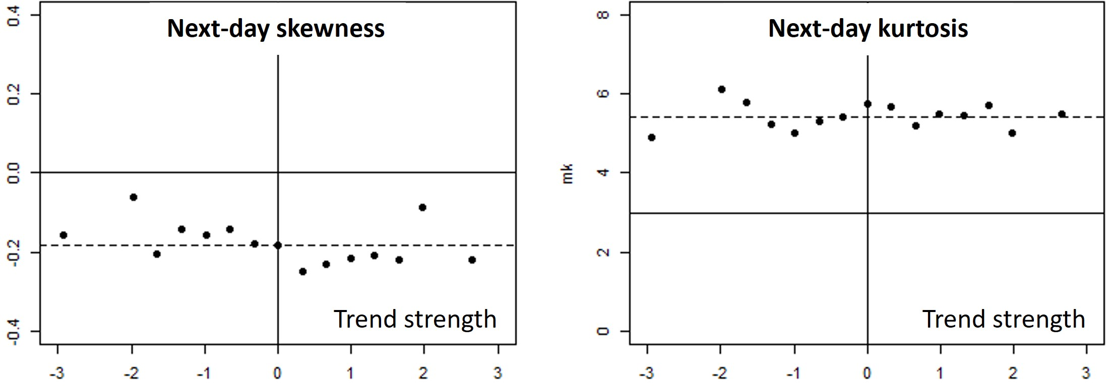
The skewness and kurtosis of the return distributions in each bin is shown in fig. 7. In the left graph, we observe an average negative skewness of \(-0.18\), reflecting the general negative skewness of financial market
returns. However, the skewness does not visibly depend on the trend strength. In the right graph, we observe an average kurtosis of \(+5.4\), which is significantly higher than the Gaussian value of 3. For comparison, a
Student’s t-distribution \(p(x)\) with \(\nu\) degrees of freedom has tails that fall off as \(\vert x\vert^{-\nu-1}\) and kurtosis \(3+6/(\nu-4)\), so our average kurtosis corresponds to a tail index of 6.5. However, there is also no visible dependence of the kurtosis on the trend strength.
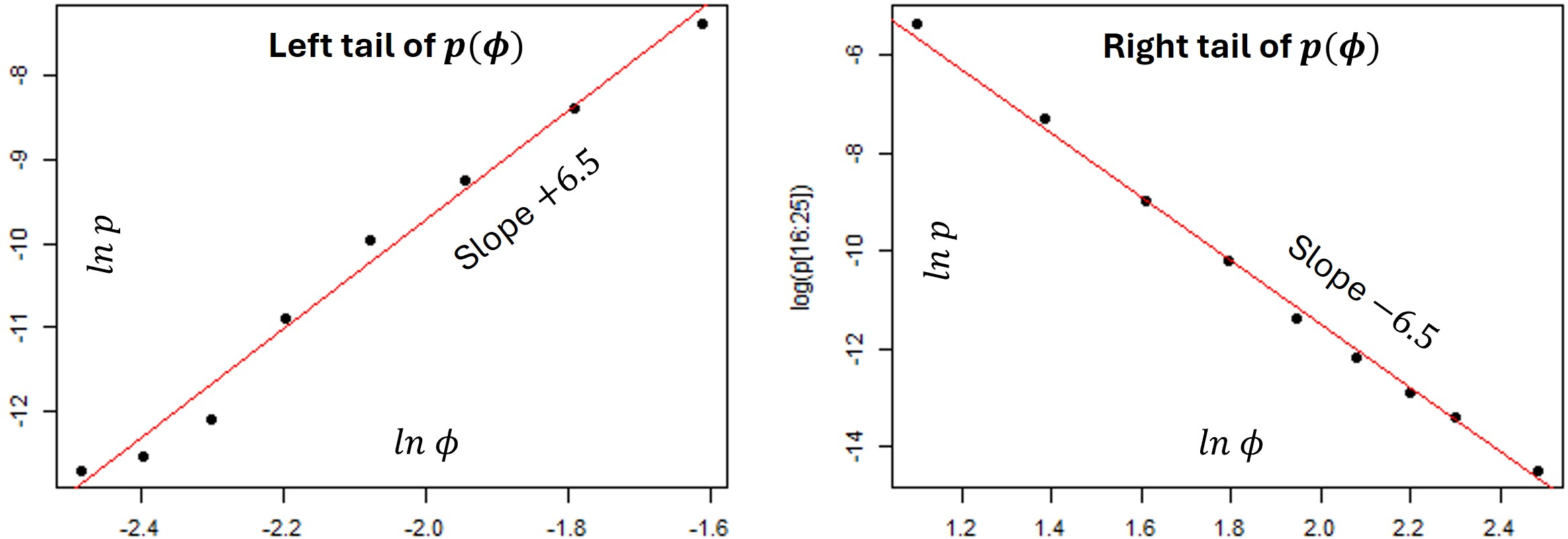
Note that this does not mean that the kurtosis of the overall return distribution \(\rho(r)\) is just \(+5.4\). This overall distribution is obtained by integrating the next-day return distribution \(\rho_\phi(r)\) for a given trend strength \(\phi\) over all \(\phi\). However, as we have seen, the variance of \(\rho_\phi(r)\) is the quadratic function (3 ) of the trend strength \(\phi\). Thus, \(\rho(r)\) is a mixture of distributions of different variances. Let the probability of trend strength \(\phi\) be \(p(\phi)\). Even if the distribution \(\rho_\phi\) was Gaussian (skewness 0, kurtosis 3) with mean 0, this integration would result in a mixed distribution with kurtosis \(>3\): \[\rho(r)=\int d\phi\;p(\phi)\;\rho_\phi(r)=\int d\phi\;p(\phi)\cdot{1\over\sqrt{2\pi}\sigma_\phi}\exp\{-{1\over2}{r^2\over\sigma_\phi^2}\} \label{mixed}\tag{6}\] Our model (3 ) and table 1 determine the variance up to a trend-independent constant \(c\): \[\sigma_\phi^2\sim\;c-0.06\phi+0.09\phi^2 \rightarrow\;(0.3\phi)^2\;\;\;\text{for}\;\;\;\vert\phi\vert\rightarrow\infty.\] Fig. 8 shows a log-log plot of \(p(\phi)\) against \(\phi\) for our data. We empirically read off: \[p(\phi)\sim\vert\phi\vert^{-\gamma}\;\;\;\text{with}\;\;\;\gamma\approx6.5,\] Changing variables from \(\phi\) to \(\phi/r\), (6 ) translates this into power-law tails of \(\rho(r)\): \[\rho(r)\sim\int d\phi\;\vert\phi\vert^{-\gamma-1}\exp\{-{1\over2}\Big({r\over0.3\cdot\phi}\Big)^2\} \sim\vert r\vert^{-\gamma}.\] Those are the tails of a Student’s t-distribution with \(\nu=\gamma-1\approx5.5\) degrees of freedom. However, the fact that \(\rho_\phi(r)\) is not Gaussian, but is already fat-tailed with kurtosis \(\approx5.4\) makes the tails of the overall distribution \(\rho(r)\) even thicker. This explains why the tail index of the overall distribution of our daily market returns is smaller, namely closer to 4.
5 Statistical-Mechanical Interpretation↩︎
Our previous results (1 ) for next-day returns have led us to develop a lattice gas model of financial markets [24], [25]. Its goal is to explain the empirically observed interplay of trends and reversion in (1 ), as well as other observed analogies between financial markets and critical phenomena, from first
principles. In this section, we show how our current results are also consistent with this lattice gas model near criticality.
Let us first briefly summarize the model, referring to [24], [25] for further explanations. The lattice represents
the social network of investors, while the gas molecules represent the shares of an asset (such as a stock) that are distributed across this network. In efficient markets [16], arbitrageurs should drive the lattice gas to its critical temperature, where the persistence of trends just goes to zero. This can be viewed as a form of self-organized criticality [32]. It is in line with the observed evolution of financial markets: trend-following no longer works as well as it used to.
The market capitalization of the stock is identified with the total number of molocules, and price-minus-value \(\hat{\pi}(t)\) is identified with the deviation of the molecule density from its critical value. If one
naively assumes a static hypercubic lattice, whose nodes and links do not change, \(\hat{\pi}(t)\) can be shown to evolve in time like the magnetization in the Ising model near its critical point: it performs a random walk
in a quartic "Landau potential" \[V(\hat{\pi})\sim a\cdot\hat{\pi}+{b\over2}\cdot\hat{\pi}^2+{c\over4}\hat{\pi}^4,\] whose derivative is (a rescaled version of) the cubic driving force (1 ). Here,
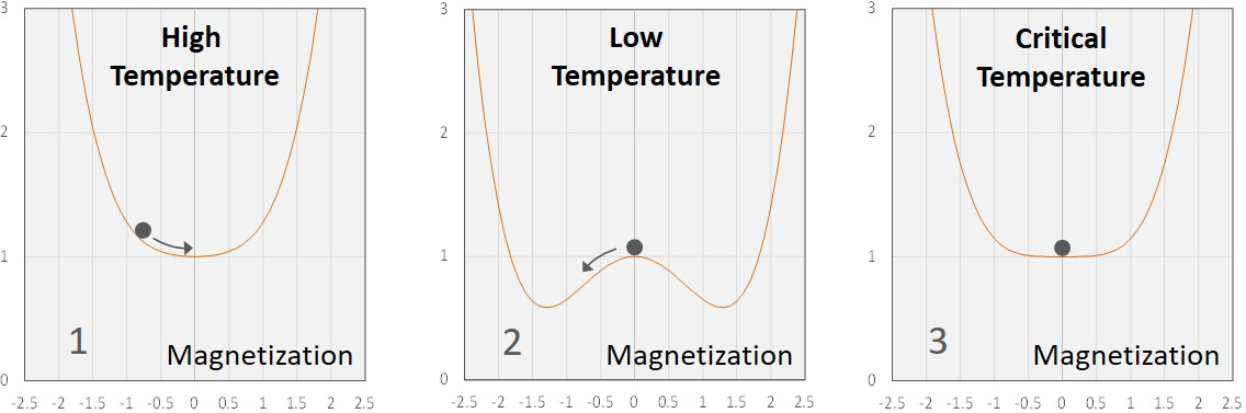
the risk premium \(a\) corresponds to a small magnetic field, the persistence \(b\) of trends corresponds to the deviation from the critical temperature, and the strength \(c\) of trend reversion is related to the renormalization group fixed point value of the coupling constant of \(\hat{\pi}^4\) field theory. At the critical point \(a=b=0\), a second-order phase transition occurs (fig. 9). Historically, \(b\) in (1 ) has been small and positive, which translates into a lattice gas slightly below its
critical temperature. This model has the potential to explain why some empirically observed phenomena in financial markets are strikingly reminiscent of critical phenomena [24].
In reality, of course, the social network is not a static hypercubic lattice but a dynamical random lattice: its nodes and links change in time. According to [25], this random network has two phases. In phase 1, it reduces to small-world network that does not lead to nontrivial critical phenomena. However, in phase 2, it is effectively described by a random surface at large
scales (in the renormalization group sense). The conformal factor \(e^{\alpha\phi}\) on this surface (for some \(\alpha\in R\)) is a new random variable, in addition to the molecule density.
It originates from a new local degree of freedom on the network: the number of links of each node.
The overall mode of the conformal factor \(e^{\alpha\phi(t)}\) measures the dynamic size of the network. For details, we refer to [25]. What is relevant in the present context is that \(\phi\) can be shown to perform a random walk in a Liouville potential. Moreover, on a random surface, some terms in the Landau
potential receive a so-called “gravitational dressing" by powers of \(e^\phi\): \[V(\hat{\pi},\phi)\sim {Q\over2}\phi+l^2e^{-\alpha\phi}
+a\cdot e^{\gamma\phi}\cdot\hat{\pi}+{b\over2}\cdot e^{\beta\phi}\cdot\hat{\pi}^2+{c\over4}\cdot \hat{\pi}^4,\] where the parameters \(\alpha,\beta,\gamma,Q\) depend on the details of the model. E.g., for the Ising
model, one obtains from the theory of random surfaces [33]–[35]: \[\alpha^2={2\over3}\;\;\;,\;\;\;{Q\over\alpha}={7\over3}\;\;\;,\;\;\;{\gamma\over\alpha}={5\over6}\;\;\;,
\;\;\;{\beta\over\alpha}={1\over3}.\] In our model, the logarithm of the conformal factor plays the role of a dynamic log-volatility in the sense that the returns (i.e., the changes of the price in time) are replaced by \[\dot{\hat{\pi}}(t)\;\rightarrow\;\dot{\pi}(t)=\dot{\hat{\pi}}(t)\cdot e^{\gamma\phi(t)},\] as in the stochastic log-volatility models mentioned in subsection 2.4. In simple stochastic log-volatility models, \(\phi\) evolves independently of \(\pi\). This cannot explain the the back-reaction of asset returns \(\dot{\pi}\) on the volatility, which is empirically
observed, e.g., in the leverage effect mentioned in section 2. However, in the lattice gas model, \(\phi\) is independent of \(\pi\) only at the critical point \(a=b=0\). Away from this point, the dynamic equations of motion for \(\pi\) and \(\phi\) follow from the purely dissipative”model A" of critical dynamics [36]: \[\begin{align}
\dot{\hat{\pi}} \sim -{\partial\over \partial\hat{\pi}} V(\pi,\phi)\;\;\;,\;\;\;
\dot{\phi} \sim -{\partial\over \partial\phi} V(\pi,\phi).\label{modelA}
\end{align}\tag{7}\] Near the critical point, \(a\) and \(b\) in the potential \(V\) are small. Then the potential for \(\phi\) has a minimum at \(\alpha\phi_0=\ln(2\alpha l^2/Q)\). Shifting \(\phi\rightarrow\phi-\phi_0\), such that the minimum lies at \(\phi_0=0\), and expanding the second equation around this minimum yields, to linear order in \(\phi\): \[\dot{\phi}\sim-{Q\over2}\phi-a\cdot c_1\pi-b\cdot
c_2\pi^2\] with some constants \(c_1, c_2\). This is precisely the form of our ansatz (4 ), with \(2\gamma\dot{\phi}\) in the role of the change of the
logarithm of the expected variance \(\ln \langle r^2_{t+1}\rangle-\ln \langle r^2_{t}\rangle\).
Of course, this only shows that the lattice gas model can, to first order, replicate the form of the dependence of the future variance on the current trends and the current variance, as quantified in this paper. It remains to theoretically work out the
signs and values of the coefficients \(c_1,c_2\) and to compare them with the measurements in this paper. To this end, the lattice gas model, which describes only a single asset, must first be generalized to other conformal
field theories that can be interpreted as models of several correlated assets. Work in this direction is in progress.
6 Summary and Conclusions↩︎
To summarize, we have supplemented the previous forecast (1 ) of expected next-day returns \(r_{t+1}\) in financial markets by analogous forecasts of the next-day variance and the next-day
correlations. While tomorrow’s expected return is modeled by a cubic polynomial in today’s trend strength \(\phi_t\), second-order polynomials in \(\phi_t\) seem to be sufficient to model
tomorrow’s variance and correlations. However, in these cases it is important to also include today’s variances \(\sigma_t^2\) and correlations \(\rho_t\) as important explanatory factors,
as both the variance and correlations are well-known to be auto-correlated and to revert to their longer-term values.
Regarding the variance, we have found that the following model yields the best out-of-sample R-squared for forecasting the square \(\langle r_{t+1}^2\rangle\) of the next-day return: \[\begin{align}
\langle r_{t+1}^2\rangle&=&a+d\cdot \sigma_t^2+e\cdot \phi_t+f\cdot \phi_t^2\;\;\;\notag\\
\text{with}&&a=0.13\pm0.04,\;\;\;d = 0.79\pm0.05,\;\;\;e = -0.06\pm0.01,\;\;\;f = 0.09\pm0.01.\notag
\end{align}\] The \(a\) and \(d\) terms are already present in common mean-reverting variance models such as [19], [26], where \(d-1\) is also negative and measures how quickly the variance reverts to its equilibrium value, which has been normalized to 1
in the above.
The \(e\) and \(f\) terms refine such models by also taking current trends into account. The positive value of \(f\) implies that the variance tends to grow
day after day in times of strong trends, which explains why it is high after trends have built up, as shown in fig. 1, right. The negative value of \(e\) shows that the variance grows faster in times of strong down-trends
as opposed to up-trends. We have found that this asymmetry is particularly strong for equities and mostly stems from short-term trends. Since trends measure cumulative recent returns, this can be interpreted as the “leverage effect": strong negative
returns tend to be followed by an increase of the variance.
However, we have also found that the alternative ansatz (4 ), in which the variance is replaced by the log-variance, also fits our empirical data well. The results can be used to refine stochastic log-variance
models such as [20], [28], [29] by also taking current trends
into account. As pointed out in section 5, this ansatz naturally arises in the recent proposal [24], [25] of modeling
financial markets by a lattice gas near its critical point. This could be an important clue in the search for a statistical-mechanical model of financial markets that can explain all stylized facts of finance [21]–[23] from first principles.
Regarding the future correlation \(\rho_{t+1}\) of two assets, we have modeled it as a polynomial of the current trend strengths \(\phi_t,\psi_t\) of the two assets, as well as today’s
correlation \(\rho_t\). We find the best out-of-sample \(R\)-squared with the quadratic polynomial \[\begin{align}
\rho_{t+1}&\sim&a+g\cdot \rho_t+o\cdot \phi_t\psi_t\;\;\;\notag\\
\text{with}&&g=0.58\pm0.03,\;\;\;o\;=\;0.026\pm0.006.\notag
\end{align}\] This ansatz should be seen as an approximation to a more complex future correlation model that ensures that correlations remain within the range\([-1,+1]\). The coefficient \(a\) reflects the average long-term correlation of the two assets and depends on the asset pair. Since \(g<1\), the correlation tends to revert to the long-term correlation. The \(o\)-term refines such models by taking trends into account. It implies, e.g., that the next-day correlation of two assets is about \(0.1-0.2\) higher (lower) than their average correlation, when
both trends are strong (\(\phi,\psi\ge2\)) and point in the same (opposite) direction.
Apart from the cross-term \(\phi\cdot\psi\), for equity markets and short trend horizons we also find significant linear and quadratic terms \((\phi+\psi),(\phi^2+\psi^2)\). They confirm
that equity markets are particularly highly correlated during crises, i.e., in times of strong down-trends.
The observation that current trends can help to predict future returns has successfully been exploited for decades by the trend-following industry. As reported here, trends are even better in predicting future risk in the sense of volatilities and
correlations. This should have equally important applications in market risk management. Moreover, combining the forecasts for future expected returns and for the covariance matrix will lead to improved methods for portfolio construction. We leave these
applications for future work.
Acknowledgements↩︎
We would like to thank Ashkan Nikeghbali, Thomas Lehéricy, Maximilian S. Janisch, Gisela Reichmuth, and Stefan Ask for discussions. This research is supported by the Swiss National Science Foundation under grant no. PT00P2_206333.
Appendix A: Markets and Data↩︎
Our analysis is based on historical daily log-returns for the set of futures markets shown in table 8. This set is diversified across four asset classes (equity indices, interest rates, currencies, commodities), three regions (Americas, Europe, Asia)
and three commodity sectors (energy, metals, agriculture).
| Table 8: Markets | America | Europe | Asia |
|---|---|---|---|
| Equities | S&P 500 | DAX 30 | Nikkei 225 |
| TSE 60 | FTSE 100 | Hang Seng | |
| Interest rates | US 10-year | Germany 10-year | Japan 10-year |
| Canada 10-year | UK 10-year | Australia 3-year | |
| Currencies | CAD/USD | EUR/USD | JPY/USD |
| GBP/USD | AUD/USD | ||
| NZD/USD | |||
| Commodities | Crude Oil | Gold | Soybeans |
| Natural Gas | Copper | Live Cattle | |
| Com.-Sectors: | Energy | Metals | Agriculture |
For all contracts, we consider 33 years of daily prices from Jan 1, 1991, to June 28, 2023. Daily prices \(P_i(t)\) were taken from Bloomberg, where \(i\) labels the asset and futures are rolled 5 days prior to first notice. Our data are a slightly updated version of the data set [37], which has been used and described in more detail in [15].
Appendix B: Methodology↩︎
B1: Trend Horizons↩︎
We consider trends with 10 different time horizons: \[T_k=2^k\;\text{business days with}\; k\in \{1,2,3,...,10\}\notag\] This represents periods of approximately 2 days, 4 days, 8 days, 3 weeks, 6 weeks, 3 months, 6 months, 1 year, 2 years, and 4 years. Thus, there are 10 different trend strengths at each point in time. A given asset may well be, e.g., in a long-term up-trend at the 1-year time scale, and at the same time in a short-term down-trend at the 3-week time scale.
B2: Definition of the Trend Strength↩︎
We define the trend strength as follows: Let \(P_i(t)\) be the daily closing price of market \(i\). We define normalized log-returns \(R_i(t)\): \[R_i(t)={r_i(t)\over \sigma_i}\;,\;\;\;r_i(t)=\ln {P_i(t)\over P_i(t-1)}\;,\;\;\;\sigma_i^2=\text{var}(r_i)\;,\;\;\;\mu_i=\text{mean}(r_i)\;,\notag\] where the long-term daily risk premium \(\mu_i\) and the long-term daily standard deviation \(\sigma_i\) of a market \(i\) are measured over a preceding 10-year period. For a given horizon \(T\) and a given market \(i\), the trend strength \(\phi_{i,T}(t)\) at the close of trading on day \(t\in Z\) is a weighted average of previous log-returns of that market in excess of the long-term risk premium: \[\phi_{i,T}(t)=\sum_{n=0}^\infty w_T(n)\cdot \hat{R}_i(t-n)\;\;\;\text{with}\;\;\;\hat{R}_i(t-n)=R_i(t-n)-{\mu_i\over\sigma_i}.\notag\] Here, \(w_T(n)\) is a weight function. We normalize it such that the trend strength \(\phi_{i,T}\) has standard deviation 1. Assuming that returns on different days are independent of each other (which is true to high accuracy), this implies: \[\sum_{n=0}^\infty w_T^2(n)=1.\notag\] With this normalization, \(\phi_{i,T}\) is the t-statistics of the trend. All trend strengths are then comparable with each other, so we can aggregate across all markets and time scales. As in [15], we use the following weight function for the trend strength \(\phi_T\): \[\begin{align} \tilde{w}_T(n)&=&M_T\cdot\;n\cdot e^{-2n/T} \;\;\;\text{with normalization factor} \;\;M_T. \notag \end{align}\] While the precise definition of the weight function does not matter much, we use this one, because it has only one single free parameter \(T\) (which reduces the risk of overfitting historical data), and because it can efficiently be computed recursively. It is essentially equivalent to a moving average cross-over, where the trend strength is proportional to the average price over a short time period \(T/6\) minus the average price over a long time period \(T\). To reduce the effect of outliers, we put a ceiling/floor on the trend strength at \(\pm 2.5\). We also put a ceiling/floor on returns that are more than 20 standard deviations from the mean.
B3: Statistical Analysis↩︎
Given the small values of many of our regression coefficients, and the huge amount of noise in financial market data, we must be very careful in assessing the statistical significance of the results. Since market returns cannot be assumed to be
independent, identically distributed normal random variables, we cannot trust standard formulas for the t-statistics, adjusted R-squared’s, and other statistics. Instead, the test statistics reported in this paper have been measured empirically as
follows:
The error of all regression coefficients (\(a,b,c,...\)) and their t-statistics are computed by bootstrapping: we draw 100 samples with replacement from the 8192 trading days covered by our analysis. Regression on these 100
samples of days yields a distribution of 100 regression coefficients. The estimation errors we report are half of the difference between the 84th and the 16th quantile of this distribution. These actual errors are typically 3-4 times as large as the errors
reported by standard regression tools, which strongly under-estimate them.
The adjusted R-squared is computed by 16-fold cross validation: we split our 8192-day time period into 16 512-day periods. We then combine 15 of these sub-periods into a training sample. This yields an out-of-sample prediction of the target variable for
the 16th period (the validation sample). Repeating this 16 times such that each sub-period appears once as the validation sample, we get an out-of-sample prediction for the target variable over the whole period. The out-of-sample R-squared \(R^2_{adj}\) that we report is the square of the correlation of this predicted target variable with the actual target variable. It is significantly further below the in-sample \(R^2\), compared
with the output of standard regression tools.
Table 1 also reports \({R}^2\) and \({R}^2_{adj}\) "aggregated across time scales". Those are based on using the equally-weighted mean of the 10 trend strengths on each day to predict the
next-day return for each market. I.e., we combine the 10 different trend factors into a single one, which has a higher predictive power than each single factor by itself.
Appendix C: Refined Correlation Regression↩︎
In the correlation regression (5 ), we have replaced tomorrow’s standard deviations \(\sigma_{t+1}, \omega_{t+1}\) by today’s standard deviation \(\sigma_t,\omega_t\) on the left-hand side. Using our previous results for (3 ) to correct this, table 9 shows that the corrected results (right) do not differ significantly from the approximate results of table 5 (shown again on the left).
| Approximate correlation regression | Corrected correlation regression | ||||||
|---|---|---|---|---|---|---|---|
| Coeff. | Value | Error | t-stat. | Coeff. | Value | Error | t-stat. |
| \(a\) | \(+0.063\) | \(0.013\) | 4.7 | \(\tilde a\) | \(+0.066\) | \(0.018\) | 3.6 |
| \(g\) | \(+0.583\) | \(0.027\) | 21.8 | \(\tilde g\) | \(+0.574\) | \(0.025\) | 22.6 |
| \(h\) | \(-0.006\) | \(0.004\) | 1.4 | \(\tilde h\) | \(-0.007\) | \(0.006\) | 1.2 |
| \(h_2\) | \(-0.001\) | \(0.001\) | 1.3 | \(\tilde h_2\) | \(-0.002\) | \(0.002\) | 0.8 |
| \(o\) | \(+0.026\) | \(0.006\) | 4.1 | \(\tilde o\) | \(+0.026\) | \(0.006\) | 4.0 |
| \(R^2\) | 0.0291 | \(R^2_{adj}\) | 0.0289 | \(R^2\) | 0.0279 | \(R^2_{adj}\) | 0.0276 |