1 Introduction↩︎

Precise timing of radio pulsars has long been proposed as a promising method of detecting gravitational waves (GWs) [1], [2]. Millisecond pulsars (MSPs), characterized by their short (\(<30\) ms) and highly stable spin periods, are particularly suitable for use in pulsar timing. To distinguish genuine GW signals from noise, it is necessary to monitor multiple pulsars (i.e., a pulsar timing array, or PTA) and analyze the correlations in their timing residuals [3], [4]. Decades of dedicated timing campaigns have improved the precision of timing residual measurements to the nanosecond (ns) level, which has recently led to the detection of a potential nanohertz GW background [5]–[9].

Pulsar discoveries are particularly efficient in globular clusters (GCs). Since the first detection of a pulsar in a GC [10], over \(330\) pulsars have been observed in these dense stellar systems ¹. Remarkably, more than \(95\%\) of these pulsars are MSPs, reflecting rich dynamical processes in GCs to spin up neutron stars. In fact, N-body simulations predict that each GC may host \(10-100\) MSPs [11]. Correspondingly, future more sensitive telescopes, such as the Square Kilometre Array (SKA), are expected to increase the total number of GC pulsars to about \(1700\) [12].

The abundance of MSPs in GCs has motivated the idea of using their timing residuals to search for compact binary GW sources within the same clusters [13]. This approach holds particular promise for probing intermediate-mass black holes (IMBHs, \(10^3-10^5M_\odot\)). They are theoretically predicted to form in GCs, and may form binaries with stellar-mass black holes (\(10M_\odot\)) or other IMBHs (see early studies such as [14]–[17] and more recent works including [18]–[26]).

However, one theoretical problem arises when an MSP is located near a GW source. The wavefront curvature becomes significant [13], [27], invalidating the plane-wave approximation. To overcome this issue, several works have extended the theory into the “near-field” regime, where the minimum distance between the GW source and the line of sight to the pulsar (this distance is called “impact parameter”, denoted by \(b\)) can be as small as a few wavelengths of the GW. It was found that in the case of small \(b\), the leading-order effect on the propagation of pulsar signals decays rapidly as \(1/b^3\) [28], [29]. Later studies recognized that this rapid decay results from assuming both the pulsar and the observer to be infinitely far from the GW source. If the pulsar is placed near the wave zone boundary, the signal can be substantially stronger [30]. This “edge effect” is relevant in realistic GC configurations where the GW wavelength could be comparable to the size of the cluster. Indeed, in this case the timing residuals can reach \(500\) ns under favorable conditions [31], [32].

Beyond the near-field challenge, the full potential of PTAs is realized when multiple MSPs are timed simultaneously. For GC MSPs, it has been suggested that combining timing data from several MSPs within the same cluster can enhance sensitivity to an isotropic GW background [33] or to GW bursts originating within the cluster [34]. Recently, a detailed near-field calculation incorporating the edge effect identified promising conditions for detecting IMBH binaries in clusters such as M15 and \(\omega\) Cen, where multiple MSPs have been found near the cluster center and could collectively achieve a timing-residual sensitivity at the microsecond (\(\mu\)s) level [35].

The idea and methodology have also been applied to MSPs in galactic centers. Earlier proposals suggested that timing MSPs near the Galactic Center could reveal a binary companion of Sgr A\(^*\) [36], [37]. The observational consequence of a curved wavefront was also studied [38], [39], though initially in a different context [40], and these studies suggest that monitoring a sample of MSPs within about \(1\) pc of Sgr A\(^*\) could yield high signal-to-noise detections of a potential binary companion. Similar analyses have been extended to MSPs in nearby galaxies such as the Large Magellanic Cloud, M31, M32, and M87, suggesting that future observations with the SKA could detect binary GW sources if MSPs within \(0.1-1\) pc of the centers are monitored over a decade [41].

In this work, we take a further step toward a comprehensive model of the PTA response to an internal GW source by incorporating four elements essential for realistic astrophysical configurations. (i) Binary eccentricity: existing models typically assume circular binaries as the GW sources, whereas dynamical simulations of star clusters favor eccentric orbits. (ii) Second-order stress-energy tensor: previous calculations (including ours [35]) sometimes retain only the lowest-order terms in the stress-energy tensor, but higher-order contributions may be equally important (e.g., see Ref. [32]). (iii) Non-radiative self-field: close to the GW source the near-field non-wave part of the strain induced by varying gravitational potential becomes non-negligible but has sometimes been overlooked in previous works. (iv) Pulsar term: the effect of GWs on the pulsar itself is often neglected but becomes important when the pulsar lies within a few GW wavelengths of the source.

The paper is organized as follows. Section 2 presents our theoretical framework, including the derivation of the timing residual in the near-field regime, the expansion of the GW strain to second order, and the calculation of the mass quadrupole moment for eccentric binaries. In Section 3, we analyze the near-field effects and compute the timing residuals for specific astrophysical systems including the GCs M15 and \(\omega\) Centauri, as well as the galactic nuclei Sgr A\(^*\) and M31. We also examine the phase differences between MSPs and discuss the detectability of the signal. Section 4 discusses our results, compares our model predictions with previous works, and presents our conclusions. The code and the numerical data used to produce the figures are available at ².

2 Near-field Timing Residual↩︎

2.1 Timing Residual↩︎

Fig. 1 illustrates the system of our interest. It includes a black-hole binary as the GW source, an MSP (emitter), and Earth (observer). The MSP and the GW source are located in a GC far from the observer with \(r_e\ll r_o\). We choose a coordinate system such that the center-of-mass of the black-hole binary is static and located at the origin. We further assume that the MSP and the Earth are also static, and their locations are \((b,0,z_e)\) and \((b,0,z_o)\), respectively. The pulses emitted by the MSP propagate along the \(z\) axis with an impact parameter of \(b\). If we consider nanohertz GWs, the wavelength is approximately \(\lambda_{\mathrm{GW}}\sim\mathrm{pc}\), comparable to the size of a typical GC. Consequently, both the MSP and the pulse signals it emits reside in the near-field zone, where the non-radiative component of the gravitational field is significant.

The passing GW perturbs the spacetime between the pulsar and the Earth, thereby causing the observed pulse arrival times to deviate from those in flat spacetime. The time difference, also known as the timing residual \(R(t)\), is given by \[\begin{align} R(t)=\int_{0}^{t}\frac{\nu_0-\nu(t_{\rm obs})}{\nu_{0}}\,\mathrm{d} t_{\rm obs}, \end{align}\] where \(\nu_0=\left.-g^{\mu\nu}K_{\mu}V_{\nu}\right|_{e}\) is the emitted frequency in the rest frame of the pulsar, and \(\nu=\left.-g^{\mu\nu}K_{\mu}V_{\nu}\right|_{o}\) is the frequency measured at the observer at the time \(t_{\rm obs}\). Here, \(g^{\mu\nu}=\eta^{\mu\nu}-h^{\mu\nu}\) denotes the perturbed metric of spacetime, \(K_{\mu}\) is the dual to the photon’s four-momentum, and \(V_{\mu}\) is the dual to the four velocity, where \(e\) and \(o\) denote the emitter (pulsar) and the Earth, respectively.

In the weak-field limit we have \(h^{\mu\nu}\ll1\), and the four-vectors take the form \(K_{\mu}=\bar{K}_{\mu}+\delta K_{\mu}\), \(V_{\mu}=\bar{V}_{\mu}+\delta V_{\mu}\). The barred vectors \(\bar{K}_{\mu}=\nu_0/c\,(-1,0,0,1)\) and \(\bar{V}_{\mu}=c\,(-1,0,0,0)\) represent unperturbed values in flat spacetime, satisfying \(-\eta^{\mu\nu}\bar{K}_{\mu}\bar{V}_{\nu}=\nu_0\).

With the above definitions, we find that in leading order, \[\begin{align} \frac{\nu_0-\nu}{\nu_0}=&\left.\frac{-h_{\mu\nu}\bar{K}^{\mu}\bar{V}^{\nu}+\bar{K}^{\mu}\delta V_{\mu}+\bar{V}^{\mu}\delta K_{\mu}}{\nu_0}\right|_{o}\nonumber\\ =&\left.\left[-h_{tt}-h_{tz}+\frac{1}{c}(\delta V_{t}+\delta V_{z})+\frac{c}{\nu_0}\delta K_{t}\right]\right|_{o}, \end{align}\] where the term \(-h_{\mu\nu}\bar{K}^{\mu}\bar{V}^{\nu}\) was neglected in our previous work [35]. For \(\delta K_{\mu}\) and \(\delta V_{\mu}\), they are governed by geodesic equations \[\begin{align} \frac{d\,\delta K_\alpha}{d\lambda}=&\frac{1}{2}h_{\mu\nu,\alpha}\bar{K}^{\mu}\bar{K}^{\nu},\\ \frac{d\,\delta V_{\alpha}}{d\tau}=&\frac{1}{2}h_{\mu\nu,\alpha}\bar{V}^{\mu}\bar{V}^{\nu}. \end{align}\] Neglecting the motion of the pulsar and the observer, we have \[\begin{align} \left.\delta K_{t}\,\right|_o=&\left.\delta K_t\,\right|_e+\frac{\nu_0}{c}\int_{z_e}^{z_o}\frac{h_{tt,t}+h_{zz,t}+2h_{tz,t}}{2}\,dz,\tag{1}\\ \delta V_{t}=&c^2\int_0^t\frac{h_{tt,t}}{2}\,dt,\qquad\delta V_{z}=c^2\int_0^t\frac{h_{tt,z}}{2}\,dt.\tag{2} \end{align}\] In Equation (1 ), \(\left.\delta K_{t}\right|_{e}\) arises from the GW perturbation of a photon just emitted from the pulsar, and can be solved from \(-\left.g^{\mu\nu}(\bar{K}_{\mu}+\delta K_{\mu})(\bar{V}_{\nu}+\delta V_{\nu})\right|_e=\nu_0\). To linear order, it is \[\begin{align} \left.\delta K_{t}\right|_{e}=\left.\frac{\nu_0}{c}(h_{tt}+h_{tz})-\frac{\nu_0}{c^2}(\delta V_t+\delta V_z)\right|_{e}. \end{align}\] The two perturbations shown in Equation (2 ) are applicable not only to the four velocity of the observer but also to that of the pulsar.

Finally, the frequency difference can be expressed using \(h_{\mu\nu}\) as \[\begin{align} \frac{\nu_0-\nu}{\nu_0}=&\int_{z_e}^{z_o}\frac{h_{tt,t}+h_{zz,t}+2h_{tz,t}}{2}\,\mathrm{d}z\nonumber\\ &+\left.\left[-h_{tt}-h_{tz}+c\int\frac{h_{tt,t}+h_{tt,z}}{2}\,\mathrm{d}t\right]\right|^{o}_{e},\label{eq:Rt} \end{align}\tag{3}\] where the first integration is along the photon’s geodesic, and the second one is along the observer’s and pulsar’s geodesics. The bracket evaluated at the observer is called the Earth term, and that evaluated at the pulsar is called the pulsar term. For the photon, we choose \(z\) and the observed time \(t_{\rm obs}\) as parameters, so the local time \(t\) is given by \(t=t_{\rm obs}-(z_o-z)/c\). The upper limits of integration in the Earth term and in the pulsar term are \(t_{\rm obs}\) and \(t_{\rm obs}-(z_o-z_e)/c\).

So far, we have shown that the complete form of the timing residual contains both the Earth and the pulsar terms. However, in the context studied in this paper, where the pulsar is relatively close to the GW source and the Earth is far from the source and the pulsar (typically satisfying \(r_o/r_e\gtrsim10^5\)), the Earth term can be neglected, so we omit it in the later calculations.

2.2 GW Strain to the Second Order↩︎

Now we evaluate the GW strain \(h_{\mu\nu}\) at a position \(\mathbf{r}\) and the local time \(t\). We start from the linearized Einstein equation \[\square \bar{h}_{\mu\nu}=-\frac{16\pi G}{c^4}T_{\mu\nu},\] where \(T_{\mu\nu}\) is the stress-energy tensor of the GW source and \(\bar{h}_{\mu\nu}=h_{\mu\nu}-\frac{1}{2}\eta_{\mu\nu}h\) is the trace-reversed GW strain. The retarded solution at \((t,\mathbf{r})\) is given by \[\bar{h}_{\mu\nu}(t,\mathbf{r})=\frac{4G}{c^4}\int\frac{T_{\mu\nu}(t-|\mathbf{r}-\mathbf{r}'|/c,\mathbf{r}')}{|\mathbf{r}-\mathbf{r}'|}\,\mathrm{d}^3\mathbf{r}',\label{eq:hretarded}\tag{4}\] where \(\mathbf{r'}\) refers to the source position, with \(|\mathbf{r'}|\) comparable to the size of the GW source. Notice that the solution is not in the transverse-traceless gauge.

In this work, the GW source is an IMBH binary on bounded Keplerian motion with a semimajor axis of \(a\). Moreover, we are interested in the case where \(|\mathbf{r}|\ge b \gg |\mathbf{r}'| \sim a\), where \(b\) is the impact parameter defined in Section 1. Under these conditions, we can Taylor expand the integrand in Equation (4 ) in different orders of \(\mathbf{r'}\), which gives

Here, we have adopted the convention that the Latin letters, such as \(i\) and \(j\), refer only to the three spatial components.

To understand the magnitudes of the time derivatives in the above equation, one can use \(\partial_tT\sim\omega T\), where \(\omega\) is the average angular frequency of the binary. Since \[\begin{align} \frac{x'}{r}\sim\frac{a}{b}\ll 1,\quad \frac{x'\partial_t}{c}\sim\frac{a\omega}{c}\sim\frac{v}{c}\ll 1, \end{align}\] where \(v\) is the typical orbital velocity of the binary, the \((n+1)\)-th term from the Taylor expansion is smaller than the \(n\)-th term by a factor of either \(x'/r\) or \(v/c\). We find that in our near-field cases the two factors \(v/c\) and \(a/b\), although small, can be comparable to each other, so we keep both the \(v/c\) and the \(a/b\) terms in our calculation.

It is important to note that besides the terms at different Taylor orders, the components of \(\bar{h}_{\mu\nu}\) are also of different orders of \(v/c\). More specifically, \(\bar{h}_{\mu\nu}\) is proportional to \(T_{\mu\nu}\) according to Einstein’s equation, and the leading terms of \(T_{\mu\nu}\) in Newtonian approximation are \[\begin{align} T_{\mu\nu}\sim\rho \begin{pmatrix} c^2&cv_i\\ cv_j&v_iv_j \end{pmatrix}. \end{align}\] Therefore, \(\bar{h}_{ij}\sim (v/c)\bar{h}_{ti}\sim(v/c)^2\bar{h}_{tt}\), i.e., the \(0\)th order term (in the Taylor expansion) of \(\bar{h}_{ij}\) is comparable to the first order term of \(\bar{h}_{ti}\) and the second order term of \(\bar{h}_{tt}\). For this reason and to be complete up to the second order of \(v/c\) or \(a/b\), in the following we retain \(\bar{h}_{ij}\) up to the leading order, \(\bar{h}_{ti}\) up to the next order, and \(\bar{h}_{tt}\) up to the second order after the leading one. This model is different from our previous one [35] in which all the \(\bar{h}_{\mu\nu}\) components only contain the leading order terms, and more similar to the original model proposed in Ref. [32]. We will show later that this difference will significantly affect the results.

Including all the terms up to the second order, we find that the integration gives \[\begin{align} \bar{h}_{tt}&=&\frac{4GM}{rc^2}+\frac{2G}{r^3c^2}\frac{3x_ix_j-r^2\delta_{ij}}{r^2}Q_{ij}\nonumber\\ &+&\frac{2G}{r^2c^3}\frac{3x_ix_j-r^2\delta_{ij}}{r^2}\dot{Q}_{ij}+\frac{2G}{rc^4}\frac{x_ix_j}{r^2}\ddot{Q}_{ij},\tag{5}\\ \bar{h}_{tz}&=&-\frac{2G}{r^2c^3}\frac{x_j}{r}\dot{Q}_{zj}-\frac{2G}{rc^4}\frac{x_j}{r}\ddot{Q}_{zj},\tag{6}\\ \bar{h}_{zz}&=&\frac{2G}{rc^4}\ddot{Q}_{zz},\tag{7} \end{align}\] where \(M=\int (T_{00}/c^2)d^3\mathbf{r}'=m_1+m_2\) is the total mass of the binary GW source, \(Q_{ij}=Q^{ij}=\int T_{00}x'^i x'^j/c^2d^3\mathbf{r}'\) is the mass quadrupole moment of the source, and we have set the total momentum \(P_i=0\) and the center of mass \(x_{c,i}=0\). Using these expressions, one can verify that \(\partial^\mu\bar{h}_{\mu\nu}=0\), which agrees with the continuity equation of \(T_{\mu\nu}\). Another useful finding is that only the second-order terms of \(\bar{h}_{tt}\) and the first-order terms of \(\bar{h}_{tz}\) are time dependent, so that even though the lower-order terms are larger, they do not affect the timing residual.

2.3 Calculating the Mass Quadrupole↩︎

Now we derive the expressions for the quadrupole terms, bearing in mind that the binary orbit can be eccentric. Given a binary with a reduced mass of \(\mu=m_1m_2/(m_1+m_2)\), a semimajor axis of \(a\), and an eccentricity of \(e\), the quadrupoles are given by \[Q_{ij}=\mu x_ix_j,\] where \(\mathbf{x}=\mathbf{x}_1-\mathbf{x}_2\) is the relative position of the two members. The orientation can be described using Euler angles, with \(\theta,\phi,\psi\) representing the nutation angle, the precession angle, and the rotation angle of the perihelion, respectively. We further assume that the orbital plane of the binary is the \(x'-y'\) plane, the center of mass coincides with the origin, and the perihelion is along the positive \(x'\)-axis. Then the coordinates \(x_i'(t)\) (\(i=1,2,3\)) in the orbital plane are related to the coordinates \(x_i(t)\) in the source frame by a rotation, \[\begin{align} \mathbf{x}=R_{1}(\phi)R_{2}(\theta)R_{3}(\psi)\mathbf{x'}\equiv R_{\rm rot}\mathbf{x'}, \end{align}\] where \(R_i\) is the rotation matrix corresponding to a Euler angle. With this coordinate transformation, \(Q_{ij}\) can be expressed as \[\begin{align} Q_{ij}=\mu (R_{\rm rot}\mathbf{x'}\mathbf{x'}^{T}R_{\rm rot}^{T})_{ij}. \end{align}\]

For an elliptical Keplerian motion, the components of \(\mathbf{x'}\mathbf{x'}^{T}\) can be decomposed into Fourier series: \[\begin{align} \mathbf{x'}\mathbf{x'}^{T}=\mathfrak{Re}(\sum_{n=0}^\infty a^2\tilde{A}_n\mathrm{e}^{\mathrm{i}n\omega t}), \end{align}\] where \(\omega=\sqrt{GM/a^3}\) is the average angular frequency of the motion. If the orbit is circular, there are only \(n=0,2\) components. In more general cases, we have \[\begin{align} \tilde{Q}_{ij}=\mu a^2\sum_{n=0}^\infty\tilde{q}_{ij,n}\mathrm{e}^{\mathrm{i}n\omega t},\label{eq:Qij} \end{align}\tag{8}\] where \(\tilde{q}_{ij,n}=(R_{\rm rot}\tilde{A}_nR_{\rm rot}^{T})_{ij}\) is the factor determined by orientation and eccentricity, and we have introduced the complex form of \(\tilde{Q}_{ij}\) for simplicity, which satisfies \(\mathfrak{Re}(\tilde{Q}_{ij})=Q_{ij}\). The explicit form of \(\tilde{A}_n\) is provided in Appendix 5.

2.4 Expression of \(R(t)\)↩︎

Having specified the system of our interest, now we can calculate the timing residual \(R(t)\) to the second order of \(v/c\) or \(a/b\). The calculation is carried out in a complex representation, and the physical results are given by the corresponding real parts. Since we are interested in the oscillating part of the timing residual, terms that do not vary with time will be neglected. Choosing \(x=b\), \(y=0\), and using Equations (5 ), (6 ), (7 ) and (8 ), we can rewrite the GW strains appearing in Equation (3 ) as \[\begin{align} h_{tt}+h_{zz}&+2h_{tz}=\frac{2\mu a^2G}{r^3c^2}\sum_{n=1}^\infty\tilde{\xi}_n\mathrm{e}^{\mathrm{i}n\omega t_r}\tag{9},\\ h_{tt}&=\frac{\mu a^2 G}{r^3c^2}\sum_{n=1}^\infty\tilde{\zeta}_n\mathrm{e}^{\mathrm{i}n\omega t_r},\tag{10}\\ h_{tz}&=\frac{\mu a^2G}{r^3c^2}\sum_{n=1}^{\infty}\tilde{\eta}_{n}\mathrm{e}^{\mathrm{i}n\omega t_r}, \end{align}\] where we have defined the dimensionless functions

From the expression of \(\tilde{\xi}_n\) we find that it scales as \(r\), so that \(h_{tt}+h_{zz}+2h_{tz}\sim O(1/r^2)\). Therefore, significant contribution to the integral only arises at small \(r\), in contrast to the conventional understanding of quadrupole terms which decay as \(O(1/r)\). For this reason, the impact of GW on light is localized.

Now we calculate the two parts of the timing residual in Equation (3 ). For the first part, using Equation (9 ) and integrating over time gives \[\begin{align} \tilde{R}_1(t)&= \frac{\mu a^2G}{c^3}\sum_{n=1}^\infty\int_{z_e}^{z_o}\frac{\tilde{\xi}_n(z)}{r^3}\nonumber\\ &\qquad\times\exp[\mathrm{i}\omega n(t-\frac{z_o-z}{c}-\frac{r}{c})]\,\mathrm{d}z. \end{align}\] For the second part, the integration operates along the pulsar’s geodesic. Actually, the integrand can be written as \[\begin{align} \frac{c}{2}(&h_{tt,t}-h_{tt,z}+2h_{tz,t})=\nonumber\\ &\frac{\mu a^2G}{c}\sum_{n=1}^{\infty}\mathrm{e}^{\mathrm{i}n\omega t} \Biggl[\frac{1}{2}\biggl(\frac{\mathrm{i}n\omega}{c}-\partial_z\biggr)\Biggl(\frac{\tilde{\zeta}_n(z)}{r^3}\mathrm{e}^{-\mathrm{i}n\omega r/c}\Biggr)\nonumber\\ &+\biggl(\frac{\mathrm{i}n\omega}{c}\frac{\tilde{\eta}_{n}(z)}{r^3}\mathrm{e}^{-\mathrm{i}n\omega r/c}\biggr)\Biggr]. \end{align}\] Integrating twice over time, the oscillating part gives \[\begin{align} \tilde{R}_{2}(t)=&-\frac{\mu a^2G}{c\omega^2}\sum_{n=1}^\infty\frac{1}{n^2}\mathrm{e}^{\mathrm{i}n\omega(t-(z_o-z_e)/c)}\nonumber\\ &\times\Biggl[\frac{1}{2}\biggl(\partial_z-\frac{\mathrm{i}n\omega}{c}\biggr)\Biggl(\frac{\tilde{\zeta}_n(z)}{r^3}\mathrm{e}^{-\mathrm{i}n\omega r/c}\Biggr)\nonumber\\ &-\biggl(\frac{\mathrm{i}n\omega}{c}\frac{\tilde{\eta}_{n}(z)}{r^3}\mathrm{e}^{-\mathrm{i}n\omega r/c}\biggr)\Biggr]\Biggr|^o_{e}. \end{align}\]

To account for systems of different parameters, such as binary mass, pulsar position, and orbital period (\(P\)), we scale length (\(r\), \(z\) and \(b\)) using the wavenumber \(k=2\pi/\lambda_{GW}=2\pi/(cP)\). Then the timing residuals can be expressed in dimensionless quantities such as \(kr\), \(kz\), and \(kb\), and the results are \[\begin{align} \tilde{R}_1(t)&=\frac{G^2m_1m_2}{ac^5}\sum_{n=1}^{\infty\nonumber}\\ &\qquad\int_{kz_e}^{kz_o}\,\mathrm{d}(kz)\,\frac{\tilde{\xi}_n(kz)}{(kr)^3}\mathrm{e}^{\mathrm{i}n(kz-kr-kz_o)}\mathrm{e}^{\mathrm{i}n\omega t}\nonumber\\ &=\mathrm{Amp}\cdot\sum_{n=1}^{\infty}\int_{kz_o}^{kz_e}\tilde{r}_{1,n}\mathrm{e}^{\mathrm{i}n\omega t}\,\mathrm{d}(kz)\tag{14}\\&=\mathrm{Amp}\cdot\sum_{n=1}^{\infty}\tilde{R}_{1,n}\mathrm{e}^{\mathrm{i}n\omega t}\tag{15}, \end{align}\] and \[\begin{align} \tilde{R}_2(t)=&\frac{G^2m_1m_2}{ac^5}\sum_{n=1}^{\infty}\frac{1}{n^2}\mathrm{e}^{\mathrm{i}n\omega t}\mathrm{e}^{\mathrm{i}n(kz-kz_o)}\nonumber\\ \times&\Biggl[\frac{1}{2}\biggl(\mathrm{i}n-\frac{\partial}{\partial(kz)}\biggr)\Biggl(\frac{\tilde{\zeta}_n(kz)}{(kr)^3}\mathrm{e}^{-\mathrm{i}n(kr)}\Biggr)\nonumber\\ &+\biggl(\mathrm{i}n\frac{\tilde{\eta}_{n}(kz)}{(kr)^3}\mathrm{e}^{-\mathrm{i}n(kr)}\biggr)\Biggr]\Biggr|^o_e\\ =&\mathrm{Amp}\cdot\sum_{n=1}^{\infty}\tilde{R}_{2,n}\mathrm{e}^{\mathrm{i}n\omega t}.\label{eq:R2t} \end{align}\tag{16}\] The scaling amplitudes are the same in both equations, \[\begin{align} \mathrm{Amp}&=\frac{G^2m_1m_2}{ac^5}\\ &\simeq\frac{0.23q~\mu{\rm s}}{(1+q)^2}\left(\frac{P}{1~{\rm yr}}\right)^{-2/3} \left(\frac{M}{10^4~M_\odot}\right)^{5/3}\\ &\simeq\frac{1.1~{\rm ms}}{(1+q)^2}\left(\frac{q}{10^{-3}}\right)\left(\frac{P}{1~{\rm yr}}\right)^{-2/3} \left(\frac{M}{10^8~M_\odot}\right)^{5/3}\label{eq:Amp}, \end{align}\tag{17}\] and it depends on the orbital period \(P\), the total mass \(M\), and the mass ratio \(q=m_2/m_1\) of the two compact objects in the binary GW source. Notice that the dimensionless function \(\tilde{R}_2(t)\) can be computed readily, and \(\tilde{R}_1(t)\) also has an analytical expression. The analytical expressions of them are presented in Appendix 6. If the binary is circular, we only need to consider the \(\tilde{R}_{1,n=2}\) and \(\tilde{R}_{2,n=2}\) terms.

3 Results↩︎

3.1 Near-field Effects↩︎

Because the pulsar in our model is close to the GW source, the wavefront is curved at the pulsar and the non-radiative self-field of the GW source is also important. To highlight these “near-field effects”, Fig. 2 shows the real part of the integrand, \(\tilde{r}_{1,n}\), which is used in the calculation of \(\tilde{R}_{1,n}\) (see Eq. (14 )). For illustrative purposes, we set \(n=2\), i.e., we assume a circular binary.

The result depends on \(kb\). When \(kb\) is small (blue curve), the function at the location of \(|kz|\lesssim 1\) can significantly exceed unity, highlighting the strong effect within a distance of one wavelength from the source. Compared to our earlier calculation (dashed curve, see Ref. [35]) where we kept only the leading term of the stress-energy tensor, the effect in the current complete model is more prominent. For a more general \(kb\) (orange or green curve), we see that the function decays as \(O(1/r^2)\) for positive \(z\), as we have discussed before. For negative \(z\), the function \(\tilde{r}_{1,2}\) is oscillating and the magnitude decreases as \(O(1/r)\). Because of the oscillation, the net contribution to timing residual is small.

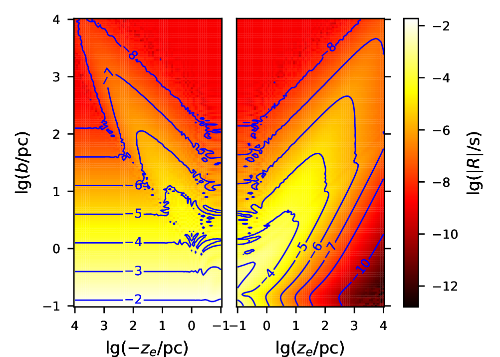
To see the net effect and its dependence on pulsar position, we show in the left panel of Fig. 3 the integrated dimensionless timing residual \(|\tilde{R}_{1,n=2}|\) as a function of \(kz_e\) and \(kb\). The observer is put at infinity. Notice that both positive and negative \(kz_e\) are considered. When \(kz_e\) is positive, the pulsar lies between the GW source and the observer, and the residual is large if both \(kz_e\) and \(kb\) are small. When \(kz_e\) is negative, the pulsar lies behind the source. In this case, as long as \(kb\) is small, the emitted light will pass closely by the GW source and produce a large timing residual (indicated by a large area with bright yellow color).

The right panel of Fig. 3 shows the dimensionless pulsar term, \(\tilde{R}_{2,n=2}\), for the same system configuration. The symmetry between positive and negative \(kz_e\) reflects the dependence on the distance \(\sqrt{b^2+z_e^2}\). This dependence is also the reason that \(|\tilde{R}_{2}|\) is large when the pulsar is close to the source. In fact, this pulsar term can be comparable to \(|\tilde{R}_1|\) even at large \(kb\), e.g., \(kb\sim10\), if one compares the two panels in Fig. 3. This result indicates that the longer the period of the GW source is, the more important the pulsar term becomes.

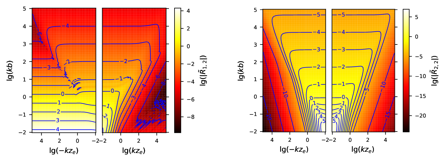
It is worth noting that when the orbital period of the GW source is long (or \(kb\) is small), our earlier assumption, that \(a/b\) is sufficiently small, may break down. To be self-consistent, we therefore require that \[\begin{align} kb\gg0.0461\left(\frac{P}{1\,\mathrm{yr}}\right)^{-1/3}\left(\frac{M}{10^8\,M_{\odot}}\right)^{1/3}. \end{align}\] In this regime, our results are accurate.

3.2 Timing Residuals for MSPs in Globular Clusters↩︎

Now we apply the complete model presented above to MSPs in GCs. We consider an IMBH binary with a total mass of \(m_1+m_2=(10^3-10^4)\,M_{\odot}\) and an orbital period of \(P=(0.1-10)\,\mathrm{yr}\). If the binary orbit is circular, the merger timescale due to GW radiation is \[\begin{align} T_{\mathrm{GW}}&\simeq\frac{a}{4|\dot{a}|}=\frac{5c^5a^4}{256G^3m_1m_2(m_1+m_2)}\\ \simeq&6.94\times10^{10}\,\mathrm{yr\,}\frac{(1+q)^2}{q}\left(\frac{M}{10^4\,M_{\odot}}\right)^{-5/3}\left(\frac{P}{1\,\mathrm{yr}}\right)^{8/3} \end{align}\] [42]. Therefore, the binary evolves slowly and remains stable over the PTA observational period. We now consider two representative GCs, M15 and \(\omega\) Cen.

M15 is a core-collapsed GC located \(10\,\mathrm{kpc}\) from Earth, with a core radius of \(r_c=0.41\,\mathrm{pc}\). The existence of an IMBH in M15 remains inconclusive given current observations, with models estimating a possible mass ranging from \(500\,M_{\odot}\) to \(4000\,M_{\odot}\) [43]–[45]. So far, 15 pulsars have been discovered in M15, and \(9\) of them are MSPs. Most pulsars are within a few core radii of M15, and some have projected distances as small as \(0.05\,r_c\). The recent timing of them has reached a precision of about \(20\,\mathrm{\mu s}\) [46], [47].

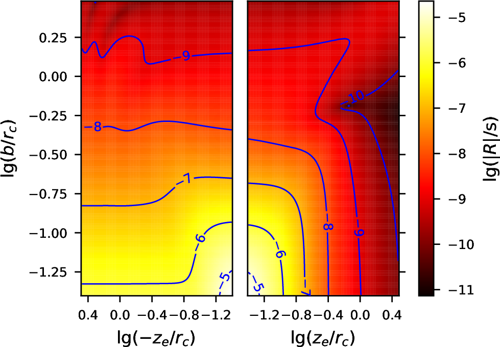
We assume that the IMBH binary in M15 has a total mass of \(m_1+m_2=4000\,M_{\odot}\), and a mass ratio \(q=1\). Within the range where our approximation holds, a longer orbital period of the binary \(P\) leads to a larger \(R(t)\). However, considering observational constraints, we assume that \(P=5\,\mathrm{yr}\) and that the orbit is circular. And we assume that MSPs are distributed within a region where \(b\geq0.04\,r_c\) and \(|z_e|\leq3\,r_c\). Moreover, we keep the orientation angles \(\theta=\pi/4\) and \(\phi=\psi=0\).

The resulting magnitude of \(R(t)\) as a function of the pulsar position is shown in Fig. 4. We find that \(R(t)\) can exceed \(100\,\mathrm{ns}\) at \(b\lesssim0.2\,r_c\), and reach \(1\,\mathrm{\mu s}\) at \(b\lesssim0.1\,r_c\). Besides, \(R(t)\) decays with increasing \(b\), and also drops rapidly for \(z_e>0\). Therefore, we conclude that the MSPs projected near the GC center, well within the core radius, are likely to exhibit a detectable timing residual, if the IMBH binary exists.

\(\omega\) Cen is the largest known GC in the Galaxy with a core radius of \(r_c=3.58\,\mathrm{pc}\). It is well-observed due to its relatively close distance of \(5.2\,\mathrm{kpc}\) from Earth. Therefore, \(\omega\) Cen is one of the best-studied GCs and is considered a prime candidate to host an IMBH in its core [48]. Observations of fast-moving stars in the central \(0.08\,\mathrm{pc}\) of \(\omega\) Cen imply a lower limit of \(8.2\times10^3\,M_{\odot}\) to the IMBH mass [49]. In contrast, studies on the motion and distribution of MSPs point to an extended central mass and put the IMBH mass below \(6\times10^3\,M_{\odot}\) [50]. A total of 18 MSPs have been discovered and confirmed in \(\omega\) Cen, most of which are located within one core radius. The smallest projected distance among them is \(0.2\,r_c\) [51]. Observations of these MSPs have achieved a timing precision of \(\sim10\,\mathrm{\mu s}\) [52].

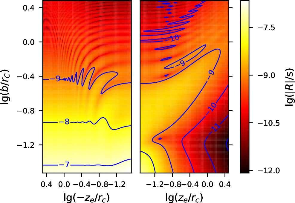
Given the uncertainties above, we take \(m_1+m_2=10^4\,M_{\odot}\) and \(q=1\). Similar to the M15 case, we assume an orbital period of \(P=5\,\mathrm{yr}\) and an orientation of \(\theta=\pi/4\). We further assume that MSPs are distributed in the range where \(b\geq0.03\,r_c\) and \(|z_e|\leq 3\,r_c\). The result is shown in Fig. 5. We see a somewhat weaker response than the M15 case at the same \(r_c\)-normalized position, mainly due to the larger core radius. Given a distance of \(0.2\,r_c\) from the center, the timing residual of an MSP is expected to reach \(\sim 10\,\mathrm{ns}\), which is much more challenging to detect than in the case of M15 MSPs.

3.3 Timing Residuals Around Sgr A\(^*\)↩︎

Now we study MSPs in the nuclei of galaxies. Sgr A\(^*\), located at the center of the Galaxy at a distance of \(8\,\mathrm{kpc}\), is an SMBH with a mass of \(4\times10^6\,M_{\odot}\) [53], [54]. Previous X-ray and \(\gamma\)-ray observations hint at a population of \(\sim10^3\) MSPs located within \(1\,\mathrm{pc}\) [55], [56]. The existence of MSPs in the Galactic Center is corroborated by a theoretical cluster-inspiral model, which predicts a population of \(\sim2.7\times10^3\) MSPs within a radius of \(20\,\mathrm{pc}\). However, according to this model, only \(\sim5\%\) of the MSPs lie in the central parsec. Of these hundreds of MSPs, approximately \(50\) are expected to be detectable by SKA, among which about \(2\) are predicted to lie within \(1\,\mathrm{pc}\) [57], [58]. Timing these pulsars can help constrain the mass and distance of the possible companion of Sgr A\(^*\).

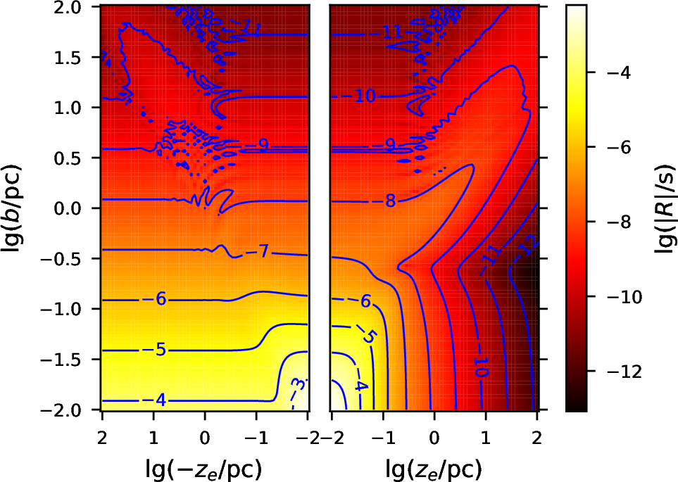
The observation of the S2 star over \(23\) yrs has excluded an IMBH companion with \(m\gtrsim400\,M_{\odot}\) at \(a\lesssim200\,\mathrm{au}\) [59]. Therefore, for our calculation, we assume that the binary has a total mass of \(m_1+m_2=4\times10^6\,M_{\odot}\), a mass ratio of \(q=10^{-4}\), and an orbital period of \(5\,\mathrm{yr}\). The merger timescale of the system is \(T_{\mathrm{GW}}\sim2.34\times10^{12}\,\mathrm{yr}\). The other parameters are set identically to those in M15. Given the above estimation of the MSPs’ distribution, we consider MSPs located at distances ranging from \(0.01\,\mathrm{pc}\) to \(100\,\mathrm{pc}\) from the binary. The result is shown in Fig. 6. We find that the MSPs within \(1\,\mathrm{pc}\) have \(R(t)\gtrsim10\,\mathrm{ns}\), and \(R(t)\) can exceed \(1\,\mathrm{\mu s}\) for the MSPs within \(0.1\,\mathrm{pc}\). At such small distances, MSPs may be accelerating due to the gravitational pull of Sgr A\(^*\). The consequence for pulsar timing will be discussed in Section 4.

3.4 Timing Residuals in M31↩︎

M31 is the nearest massive spiral galaxy, located at a distance of \(765\,\mathrm{kpc}\) from Earth. Observations indicate that M31 hosts an SMBH in the center with a mass within the range of \((0.5\sim1.4)\times10^8\,M_{\odot}\) [60], [61]. Although the current observations have not resolved any individual pulsar in M31, simulations suggest that telescopes such as FAST and SKA have the potential to detect MSPs there [62].

We assume that the SMBH binary in M31 has a total mass of \(m_1+m_2=10^8\,M_{\odot}\), a mass ratio of \(q=0.01\), and an orbital period of \(P=3\,\mathrm{yr}\). Other parameters are set identically to those in M15. The merger timescale of the system is \(T_{\mathrm{GW}}\sim2.86\times10^7\,\mathrm{yr}\). We consider MSPs located at distances ranging from \(0.1\,\mathrm{pc}\) to \(10\,\mathrm{kpc}\) from the center of M31. The timing residuals are shown in Fig. 7. Due to the binary’s large mass, the emitted GWs are strong enough to produce significant timing residuals (\(\gtrsim 1\,\mathrm{\mu s}\)) even for an MSP located at \(1\,\mathrm{kpc}\) from the center. Moreover, \(R(t)\) can reach \(\gtrsim1\,\mathrm{ms}\) for an MSP with \(b\lesssim1\,\mathrm{pc}\). The magnitudes of these timing residuals qualitatively differ from those derived in the absence of non-radiative self-fields or pulsar terms [41]. Our results suggest that finding MSPs in M31 and timing them can help us effectively constrain the binarity of the central SMBH.

3.5 Phase Difference Between MSPs↩︎

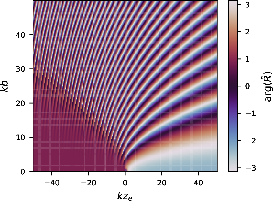
PTAs detect GWs by revealing correlated patterns in the timing residuals of different pulsars. Therefore, not only are the magnitudes of the timing residuals at different positions important, but also their phase differences.

Fig. 8 shows how the relative phase depends on pulsar positions. The bottom-left and bottom-right corners of the plot show small variation. The cause can be found in Fig. 2, which shows that the GW effect is concentrated around \(kz\approx0\) for small \(b\). Therefore, outside this central region, the phase and magnitude of the timing residual are largely insensitive to the value of \(z_e\). The rest part of the plot shows regular, stripe-like patterns. These stripes are more densely spaced in the region \(z_e<0\) than in \(z_e>0\), because when \(z_e<0\), the light is traveling in a direction opposite to the propagation direction of the GW so that the integrand \(\tilde{r}_{1,n=2}\) is more oscillatory.

4 Discussion and Conclusion↩︎

Motivated by (i) the abundance of MSPs in GCs, (ii) the observational prospect of discovering MSPs in the centers of the Milky Way and M31, and (iii) the theoretical expectation that binary GW sources reside in these dense stellar systems, we investigate the response of an array of MSPs to a GW source inside the PTA. Our work completes the earlier ones by integrating four ingredients in the same model: (i) eccentricity of the binary, (ii) second-order stress-energy tensor, (iii) non-radiative self-field of the binary, and (iv) the pulsar term. They are essential for modeling a realistic system, especially when the pulsar is only a few wavelengths away from the GW source.

Recent works sometimes neglect the pulsar term and the self-field close to the GW source [34], [38]. In this case, the timing residual is affected only by the far-field wave-like component during the propagation of the pulse. By averaging over the pulsar direction on a sphere of radius \(r_e\) (centered on the source) and over source orientation, we find that the residual is proportional to \(1/r_e\), or more specifically \[\begin{align} \langle R\rangle\sim\bar{\chi}\frac{h_o}{\omega}=0.365\times4\,\frac{\mathrm{Amp}}{kr_e}, \end{align}\] where \(\bar{\chi}=0.365\,r/r_e\) is a factor that represents the geometric effect of the relative position of the MSP and the source when \(r\gg r_e\), and \(h_o\) is the characteristic strain at the observer [38]. This result, derived from a simplified model, is more or less consistent with our model prediction when \(kr_e\gg10\), as is shown in Fig. 9 where \(\alpha\) represents the angle between \(\mathbf{r_o}\) and \(\mathbf{r_e}\). However, when \(kr_e<10\), our full model predicts a much steeper rise (between \(1/r_e^2\) and \(1/r_e^4\)) of timing residual than \(1/r_e\), highlighting the importance of the pulsar term and the self-field. Notice that when \(\alpha\simeq\pi\), significant difference can appear at a place as far as \(kr_e\sim10^3\), indicating that the near-field effect is more prominent for those MSPs behind the GW source.

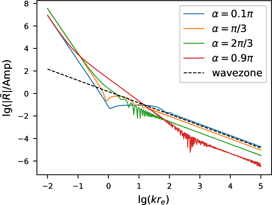
The dependence of timing residual \(R(t)\) on \(M\) and \(q\) is given directly by Eq. (17 ). However, it is worth noting that although the binary’s period \(P\) appears in Eq. (17 ), the dependence of \(R(t)\) on \(P\) is not fully captured by \(\mathrm{Amp}\) alone. Besides the scaling amplitude, the dimensionless distance \(kr=2\pi r/cP\) which appears in other terms is also \(P\)-dependent. Therefore, the proper scaling of \(P\) must also include the dependence of \(R(t)\) on \(kr\) shown in Fig. 9. The dependence evolves from \(R(t)\propto P^{1/3}\) at far field to \(P^{10/3}\) at near field.

Applying our model to GC systems such as M15 and \(\omega\) Cen, as well as the nuclei of the Milky Way and the nearby galaxy M31, we find that for MSPs located within the near field regime, the timing residual can reach \(100\,\mathrm{ns}\) to \(\mathrm{\mu s}\) in GCs, and \(\mathrm{\mu s}\) to \(\mathrm{ms}\) in galactic centers. The exact value depends on source mass and scaled distance. For comparison, the timing residuals induced by the same GW sources on the MSPs in the Galactic field (conventional PTA) fall in the range of \(10^{-3}-10\) ns because the characteristic strain is of the order \(10^{-20}\sim10^{-16}\). Detecting such signals is challenging using conventional PTA method. This comparison highlights the advantage of using a miniature PTA in a star cluster or galactic nucleus to detect potential GW sources inside the same system.

According to our previous work [35], detecting a binary GW source in a star cluster with false alarms less than \(5\%\) requires that the amplitude of the timing residual should reach \(A\gtrsim4.65\sigma/\sqrt{NN_p}\), where \(N_p\) is the number of MSPs in the near field (in the same stellar cluster), \(N\) denotes the total number of measurements, and \(\sigma\) is the precision of each measurement. If we assume \(10\) MSPs in the cluster and a total of \(100\) measurements over an observational period of five years, a measurement precision of about \(\sigma\lesssim6.8\,\mathrm{\mu s}\) will enable us to detect a signal of \(A=1\,\mathrm{\mu s}\). Interestingly, such a precision is becoming achievable in recent years in timing observations of MSPs in GCs (e.g., [63]–[65]). A longer observational period will further enhance the detectability by increasing \(N\).

In our calculation we have assumed that the MSPs are not moving relative to the GW source. However, those close to the source may undergo Keplerian motion and show additional timing residuals. For such an MSP, due to the gravity of the nearby GW source, the orbital period \(P_{\mathrm{orb}}\) around the GW source and the time derivative of the MSP’s apparent spin period \(P_{\mathrm{app}}\) are given by \[\begin{align} P_{\mathrm{orb}}\simeq&3.1\times10^4\,\mathrm{yr}\,\left(\frac{r_{e}}{0.01\,\mathrm{pc}}\right)^{3/2}\left(\frac{M}{10^4\,M_{\odot}}\right)^{-1/2}\\ =&9.7\times10^3\,\mathrm{yr}\,\left(\frac{r_{e}}{1\,\mathrm{pc}}\right)^{3/2}\left(\frac{M}{10^8\,M_{\odot}}\right)^{-1/2}, \end{align}\] where \(r_e\) denotes the average distance from the MSP to the GW source. According to the above estimations, an MSP over a typical observational period of five years has approximately a constant velocity \(v\), corresponding to a constant Doppler shift \(\Delta\nu\). This induces a linear, non-periodic accumulation in \(R(t)\), which can be removed from the timing model.

In the future, as the sensitivity of radio telescopes improves, a microsecond-level timing residual may become detectable for the MSPs in GCs and galactic nuclei. Then the model developed here will enable direct constraints on the binarity of the intermediate-mass and supermassive black holes in these systems, revealing GW sources that would otherwise remain invisible to traditional PTA analyses.

5 Expressions of orientation factors↩︎

The rotation matrices are given by \[\begin{align} &R_3(\psi)= \begin{pmatrix} \cos\psi&-\sin\psi&0\\ \sin\psi&\cos\psi&0\\ 0&0&1 \end{pmatrix},\\ &R_2(\theta)= \begin{pmatrix} 1&0&0\\ 0&\cos\theta&-\sin\theta\\ 0&\sin\theta&\cos\theta \end{pmatrix},\\ &R_1(\phi)= \begin{pmatrix} \cos\phi&-\sin\phi&0\\ \sin\phi&\cos\phi&0\\ 0&0&1 \end{pmatrix}. \end{align}\]

For a Keplerian motion in the \(x-y\) plane, \(\mathbf{x}'\mathbf{x}'^{T}\) can be written in the form of a Fourier series: \[\begin{align} \mathbf{x'}\mathbf{x'}^{T}&= \begin{pmatrix} x'^2&x'y'&0\\ x'y'&y'^2&0\\ 0&0&0 \end{pmatrix}=\mathfrak{Re}(\sum_{n=0}^\infty a^2\tilde{A}_n\mathrm{e}^{\mathrm{i}n\omega t}). \end{align}\]

In our case, the nonzero components of \(\tilde{A}_n\) are given by [66] \[\begin{align} \tilde{A}_{xx,n}&=\frac{1}{n}[J_{n-2}(ne)-J_{n+2}(ne)\nonumber\\&\qquad\qquad\quad-2e(J_{n-1}(ne)-J_{n+1}(ne))],\\ \tilde{A}_{yy,n}&=\frac{1-e^2}{n}[J_{n+2}(ne)-J_{n-2}(ne)],\\ \tilde{A}_{xy,n}&=\tilde{A}_{yx,n}=-\mathrm{i}\frac{\sqrt{1-e^2}}{n}[J_{n+2}(ne)+J_{n-2}(ne)\nonumber\\&\qquad\qquad\quad-e(J_{n+1}(ne)+J_{n-1}(ne))], \end{align}\] where \(J_n\) is the \(n\)-th order Bessel function of the first kind.

6 Analytical form of \(\tilde{R}(t)\)↩︎

Here we show the analytical expression of \(\tilde{R}(t)\) from Eq. (15 , 16 , 11 , 12 , 13 ). The complex amplitude \(\tilde{R}_{1,n}\) is given by \[\begin{align} \tilde{R}_{1,n}=\int_{kz_e}^{kz_o}\,\mathrm{d}(kz)\frac{\tilde{\xi}_n(kz)}{(kr)^3}\mathrm{e}^{\mathrm{i}n(kz-kr-kz_o)}\label{eq:R1n}. \end{align}\tag{18}\]

To integrate analytically, it is more convenient to introduce a dimensionless variable \(x\) and a scale factor \(\beta\), defined by \[\begin{align} x=&\frac{\omega}{c}(\sqrt{z^2+b^2}-z)=kr-kz,\\ \beta=&\frac{\omega b}{c}=kb=\left.\frac{v}{c}\right/\frac{a}{b}, \end{align}\] and Eq. (18 ) becomes \[\begin{align} \tilde{R}_{1,n}=\int_{x_o}^{x_e}\frac{4x\tilde{\xi}_n(x)}{(x^2+\beta^2)^2}\exp[-\mathrm{i}n(x+kz_o)]\,\mathrm{d}x. \end{align}\]

We can rewrite \(\tilde{R}_{1,n}\) by separating the orientation factor \(\tilde{q}_{ij,n}\): \[\begin{align} \tilde{R}_{1,n}=\sum_{ij}[\tilde{U}_{ij,n}(x_e)-\tilde{U}_{ij,n}(x_o)]\tilde{q}_{ij,n}, \end{align}\] and the nonzero components of \(\tilde{U}_{ij,n}(x)\) are

which is equivalent to the results in [32].

Similarly, for \(\tilde{R}_{2,n}\) we have \[\begin{align} \tilde{R}_{2,n}&=-\frac{\mathrm{e}^{\mathrm{i}n(kz-kz_o-kr)}}{2n^2(kr)^3}\biggl[\biggl(\mathrm{i}n \biggl(\frac{kz}{kr}+1\biggr)\nonumber\\ &\qquad\qquad+3\frac{kz}{(kr)^2}\biggr)\tilde{\zeta}_n -\partial_{kz}\tilde{\zeta}_n+2\mathrm{i}n\tilde{\eta}_{n} \biggr]\Biggr|^{e}_{o}\\ &=\sum_{i,j}[\tilde{V}_{ij,n}(z_e)-\tilde{V}_{ij,n}(z_o)]\tilde{q}_{ij,n}, \end{align}\] and the nonzero components of \(\tilde{V}_{ij,n}(z)\) are

This result differs from Eq. (8) in [32] by an additional term \(3(\frac{b^2}{r^2}\dot{Q}_{xx}+\frac{z^2}{r^2}\dot{Q}_{zz}+2\frac{zb}{r^2}\dot{Q}_{zx})/(2r^2)\).

References↩︎

---

1. Pulsars in GCs: https://www3.mpifr-bonn.mpg.de/staff/pfreire/GCpsr.html↩︎

2. https://github.com/HouyuanQi/PTA-Near_field_timing_residual↩︎