A Stochastic-Thermodynamic Constraint on the Seasonal Phase Locking of the El Niño–Southern Oscillation
June 18, 2026
1 Introduction↩︎
The El Niño–Southern Oscillation (ENSO) is the dominant mode of interannual variability in the tropical Pacific and influences the global atmosphere and ocean [1]–[4]. ENSO is characterized by sea surface temperature anomalies (SSTAs) in the eastern equatorial Pacific, which tend to peak in boreal winter during El Niño and La Niña (the warm and cold phases of ENSO, respectively). This seasonal peak, known as phase locking, remains a key challenge for climate models to reproduce [5]–[7] and motivates a deeper understanding of the underlying dynamics.
The recharge oscillator [8] is an idealized model widely used to study the temporal evolution of ENSO, including phase locking; for recent reviews, see [9] and [10]. With its parameters estimated from observational or climate model data, the RO is inferred to be a damped oscillator driven by stochastic noise [11]–[17], although robustly distinguishing a damped from a self-sustained regime may be difficult [18]. In this realistic parameter regime, the seasonality of the SSTA growth rate is considered the dominant cause of phase locking [5], [12]–[17], [19]. Other factors include the seasonality of the oscillation frequency [12], [15], [20], external forcing by the annual cycle [13], and nonlinearity [14], [16], but none has been well established as the dominant factor. The former two are omitted in most recent RO formulations, whereas the remaining factor, nonlinearity, is still necessary to reproduce the asymmetry between El Niño and La Niña [14], [16], [17].
[16] (hereafter ) examined the noise-driven RO and proposed the seasonal energy index (SEI) as a diagnostic measure of phase locking. In the noise-driven RO (stochastic RO; SRO), phase locking is reflected in the seasonality of SSTA variance: ENSO events peak in boreal winter, when the variance is largest. To analyze this seasonality, noted that the SRO has two degrees of freedom and interpreted SSTA as momentum in classical mechanics. In this analogy, the SSTA variance corresponds to kinetic energy. They showed that the time-integrated growth rate determines the seasonal modulation of SSTA variance and defined the SEI based on this integral (see also Fig. 1). However, the SEI is mainly discussed from a deterministic viewpoint, and a stochastic analysis of phase locking remains less developed in the SRO.
Such a stochastic analysis is naturally framed in terms of entropy, whose production quantifies the irreversibility of a stochastic process [21]. In general, energy and entropy impose distinct constraints on a physical system: energy is required to drive a change, whereas entropy governs whether the change is possible. For the SRO, a damped oscillator driven by stochastic noise, phase locking should therefore be subject not only to an energy constraint but also to an entropy-based constraint. Quantifying such a constraint requires a framework that connects entropy production to fluctuations.
Over the past two decades, the study of fluctuations in nonequilibrium systems has advanced within the framework of stochastic thermodynamics [22]–[25]. Despite its name, this framework also applies to nonthermal systems and can be used for multivariable nonlinear systems driven by stochastic noise. Such noise is present in climate dynamics, where small-scale motions in the atmosphere and ocean can be modeled as stochastic forcing [26], [27], and thus stochastic thermodynamics may be applicable. Indeed, [28] applied this framework to interannual-to-decadal synchronization between the Gulf Stream and the Kuroshio [29] and suggested that information-to-energy conversion [30], [31] may occur even in the climate system. Such new physical insights may emerge through stochastic thermodynamics, but this framework is relatively new and has hardly been used in climate research.
We analyze the SRO using stochastic thermodynamics and show that ENSO phase locking is constrained by the partial entropy production rate, which quantifies irreversibility. Section 2 introduces a linear SRO and its parameter values. Section 3 reviews a thermodynamic uncertainty relation (TUR), a fundamental inequality in stochastic thermodynamics that bounds the magnitude of fluctuations in stochastic systems [32]. Section 4 applies the TUR to the SRO, and Section 5 then discusses the implications for real ENSO. Finally, Section 6 presents the conclusions.
2 Linear stochastic recharge oscillator (SRO)↩︎
We use the following linear SRO [10]: \[\begin{align} \frac{{\rm d} T(t)}{{\rm d} t}&=R(t) T(t)+F_1 h(t)+\sigma^T \xi^T(t), \tag{1}\\ \frac{{\rm d} h(t)}{{\rm d} t}&=-\varepsilon h(t)-F_2 T(t)+\sigma^h \xi^h(t), \tag{2}\\ R(t)&=R_0 - R_a \sin(\omega t + \phi), \tag{3}\\ \left\langle\xi^T(t)\xi^T(t')\right\rangle &= \left\langle\xi^h(t)\xi^h(t')\right\rangle = \delta(t-t'), \tag{4}\\ \left\langle\xi^T(t)\xi^h(t')\right\rangle &= 0,\tag{5} \end{align}\] where \(T\) denotes the SSTA in the eastern equatorial Pacific, and \(h\) denotes the thermocline depth anomaly over the entire equatorial Pacific, corresponding to ocean heat content. The Gaussian white noises \(\xi^T\) and \(\xi^h\) are mutually independent, and the angle brackets \(\langle \cdot \rangle\) denote the ensemble average over noise realizations. All coefficients are constant except \(R(t)\). The SSTA growth rate \(R(t)\) encapsulates multiple physical processes, including the Bjerknes feedback [9]. It has an annual cycle that peaks around September (Fig. 1). The parameter \(R_0\) is the annual mean, and \(R_a\) is the amplitude of the annual-cycle component. We discuss causes of the annual cycle in \(R(t)\) later (Section [5]5.1). Our notation follows a recent review [10]. We may also write the time \(t\) as a subscript when there is no confusion, following the convention for stochastic processes [e.g., \(R_t = R(t)\)].
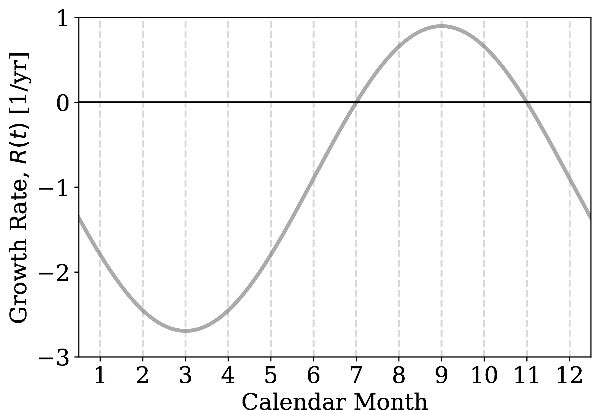
The parameters of the linear SRO are taken from , [10], or [17] (Table ¿tbl:table:sro-parameters?). The parameter set is our main case, whereas the other two sets are used to test the robustness of our results. These parameters were obtained mainly by fitting to observational or reanalysis data; [17] additionally estimated them through parameter-sweep experiments. Here, we use only the parameter values that appear in the linear SRO [Eqs. (1 )–(5 )], not those of any additional terms [17].
| KA21 | V25 | H26 | |
|---|---|---|---|
| \(T\) region | central–eastern | eastern | eastern |
| \(h\) region | basinwide | basinwide | western |
| \(R_0\) [1/yr] | \(-0.898\) | \(-1.13\) | 0.360 |
| \(R_a\) [1/yr] | 1.80 | 2.26 | 1.92 |
| \(\omega\) [1/yr] | 6.28 | 6.28 | 6.28 |
| \(\phi\) [rad] | 0.262 | 0.262 | 0.262 |
| \(F_1\) [K/m/yr] | 0.242 | 0.190 | 0.180 |
| \(\varepsilon\) [1/yr] | 0.379 | 0.380 | 1.56 |
| \(F_2\) [m/K/yr] | 11.0 | 17.6 | 17.4 |
| \(\sigma^T\) [K yr\(^{-1/2}\)] | 0.797 | 2.22 | 0.610 |
| \(\sigma^h\) [m yr\(^{-1/2}\)] | 5.82 | 14.4 | 5.54 |
| BWJ Index (Re Part) [1/yr] | \(-0.638\) | \(-0.755\) | \(-0.600\) |
| BWJ Index (Im Part) [1/yr] | 1.61 | 1.79 | 1.49 |
| Intrinsic Period [yr] | 3.90 | 3.51 | 4.23 |
In Table ¿tbl:table:sro-parameters?, the Bjerknes–Wyrtki–Jin (BWJ) index represents the eigenvalues of the SRO coefficient matrix at \(R(t) = R_0\) [9], [33], [34]. The eigenvalues are complex numbers with negative real parts. Thus, the SRO is a damped oscillator driven by stochastic noise. Indeed, even with a time-dependent \(R(t)\), the system relaxes toward \(T=h=0\) when the noise amplitudes are zero (\(\sigma^T=\sigma^h=0\)). Although \(R(t)\) can become positive and amplify \(T\) through the \(R(t)T\) term in Eq. (1 ), this effect is not sufficient to drive the SRO.
The three parameter sets differ mainly in the noise amplitudes and in the values of \(R_0\) and \(\varepsilon\) (Table ¿tbl:table:sro-parameters?). The noise amplitudes \(\sigma^T\) and \(\sigma^h\) of [10] are about three times as large as those of and [17]. Moreover, uses a positive \(R_0\) and an \(\varepsilon\) value that is about four times as large as those of and . This difference arises because defines \(h\) as the thermocline depth anomaly in the western equatorial Pacific, whereas and define it over the entire equatorial Pacific; see for a discussion of this choice. Despite these differences, all three parameter sets yield similar results in the analyses below, suggesting that our results are not sensitive to the choice of \(h\) or to the specific parameter values. The case of the parameter set, in which \(h\) is taken in the western equatorial Pacific, is discussed in Appendix C.
In the linear SRO, El Niño and La Niña are symmetric (e.g., ). By linearity, the sign-reversed state \((-T, -h)\) is also a solution; thus, the statistical properties of local maxima and minima are identical. Although nonlinear terms are necessary to model the El Niño–La Niña asymmetry [14], [17], their effects are not dominant in reproducing phase locking [14]. Hereafter, we focus mainly on El Niño events (that is, local maxima of \(T\)) and refer to the linear SRO simply as the SRO.
Our numerical setup follows . The unit of time is one model year of 360 days (30 days per month). Numerical integration was performed with the Euler–Maruyama method, using a time step of 1 day (\(=1/360\) yr). The initial conditions were set to \(T = 0\) K and \(h = 10\) m, although the results are not sensitive to this choice. Similar results were obtained for Gaussian random initial conditions, because the influence of the initial state decays rapidly under stochastic noise. The integration length and ensemble size differ across experiments and are given in each figure caption. We used sufficiently long integrations and large ensembles so that the results are insensitive to these choices. All results can be reproduced with our public code (see Data Availability).
We first confirm that the SRO simulation results are similar to those in . For comparison, we also numerically integrated a stationary SRO with constant growth rate \(R(t) = R_0\). Each integration was run for 200 years with 10,000 ensemble members. Figure 2 shows the last 5 years of one ensemble member (thin lines) together with the standard deviation across all members (thick lines). For the single member shown, \(h\) leads \(T\), and \(T\) tends to increase after the thermocline has deepened. A lagged-correlation analysis using the ensemble confirms that \(h\) tends to lead \(T\) in both the steady and unsteady SRO (not shown). The standard deviations also vary seasonally: that of \(h\) peaks around May and that of \(T\) around November. Between these times, both \(h\) and \(T\) tend to be positive, which is reflected in the maximum of the covariance \(\left\langle T h \right\rangle\) around August. These results suggest that the SRO models the phase evolution of ENSO well [10].
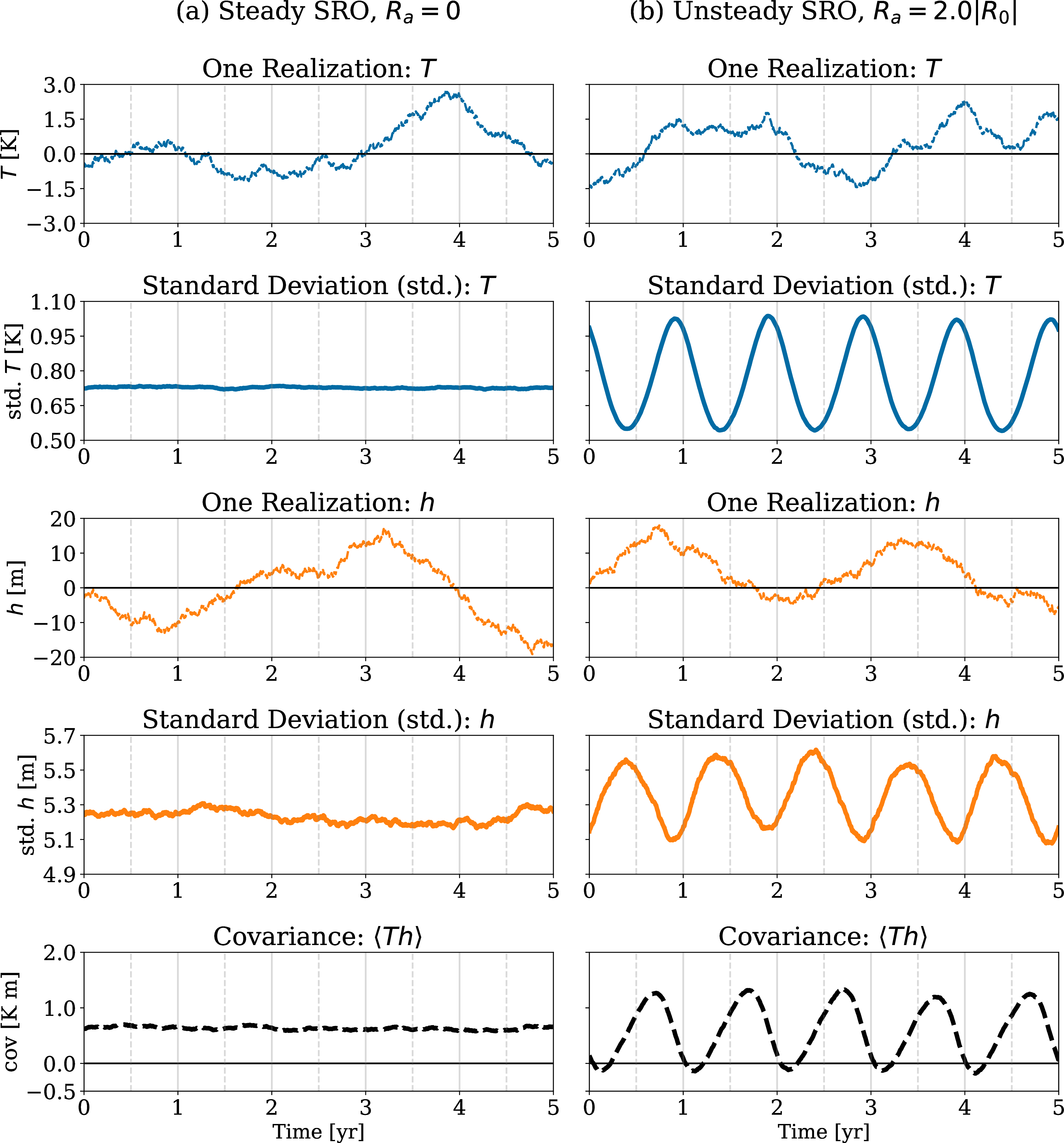
A common measure of phase-locking strength is the seasonal variance (or standard deviation) of \(T\) [12]–[14]. When the growth rate is constant, the standard deviation of \(T\) relaxes to about 0.7 K (Fig. 2a), consistent with Fig. 1e of . As \(R_a\) increases, an annual cycle emerges in the standard deviation of \(T\). For \(R_a = 2.0 \lvert R_0 \rvert\), the standard deviation of \(T\) reaches a maximum of about 1.0 K around November (Fig. 2b), consistent with Fig. 1f of . This seasonal standard deviation corresponds to the concentration of El Niño peaks in a particular season and serves as a phase-locking strength index. Indeed, although \(T\) driven by stochastic noise does not exhibit exact periodicity, its peaks tend to concentrate in November–December (Section 4). In this study, we apply stochastic thermodynamics to the SRO and examine the seasonal variance of \(T\).
3 Thermodynamic uncertainty relation (TUR)↩︎
Stochastic thermodynamics investigates the fundamental properties of fluctuations in nonequilibrium systems [22]–[25]. Despite its name, it also applies to nonthermal systems. In fact, the fluctuation theorem, which plays a central role in stochastic thermodynamics, can hold for general nonlinear stochastic systems [35]. As an important consequence of the fluctuation theorem, thermodynamic uncertainty relations (TURs) have been actively studied in recent years [32], [36]–[38]. Applying a TUR to the SRO yields the following inequality for the variance of \(T\): \[\frac{\dot{\cal P}}{2} \ge \frac{1}{\left(\sigma^T\right)^2\left\langle T^2 \right\rangle} \left( \frac{1}{2} \frac{{\rm d}}{{\rm d}t} \left\langle T^2 \right\rangle \right)^2.\] This section introduces this inequality and describes its terms, including the partial entropy production rate \(\dot{\cal P}\).
TURs are regarded as fundamental inequalities that can hold even for multivariable nonlinear systems or systems driven by multiplicative noise [39], [40]. The specific form of the inequality, however, depends on the problem setting; for details, see a review and subsequent studies [32], [40], [41]. Applied to the SRO, the above inequality means that \(\dot{\cal P}\) provides an upper bound on the squared tendency of \(\left\langle T^2 \right\rangle\), normalized by \(\left(\sigma^T\right)^2\) and \(\left\langle T^2 \right\rangle\). The partial entropy production rate \(\dot{\cal P}\) reflects the system’s irreversibility (Sections [3]3.1 and 4). Thus, this inequality links irreversibility to the seasonal variance.
We review a TUR for the subsystem \(T\) of the full \((T,h)\) state [40]. After introducing the general form of the TUR (Section [3]3.1), we discuss the specific form used in this study (Section [3]3.2). We then describe limitations of the TUR-based analysis (Section [3]3.3). Both the general and specific forms are re-derived in Appendix A. [40] obtained a TUR for time-integrated currents and argued that an instantaneous form, without time integration, can be obtained from it. Alternatively, we use a short-time-limit method [41] and show that this instantaneous TUR can be derived directly (Appendix A).
3.1 General form of the TUR↩︎
In general, TURs describe how the uncertainty of a current (defined below) is lower bounded by entropy production [32]. Reducing this lower bound requires increasing entropy production. Following [40], we apply the TUR to the subsystem \(T\) (the full system consists of \(T\) and \(h\)).
We first introduce the current \({\cal J}\) associated with \(T\): \[\begin{align} {\cal J} := g(T,h) \circ {\rm d}T, \end{align}\] where \(g(T,h)\) is an arbitrary weight function. In this subsection, we do not restrict the form of \(g\), so the TUR is general. A specific choice, \(g = T\), is discussed in Section [3]3.2. Stochastic-thermodynamic quantities are denoted by calligraphic symbols (e.g., \({\cal J}\)). The symbol \(\circ\) denotes the Stratonovich product, defined as follows [42]: \[g(T,h) \circ {\rm d} T := \lim_{{\rm d} t \rightarrow 0} \frac{g(T_{t+{\rm d} t},h_{t+{\rm d} t}) + g(T_{t}, h_{t})}{2} \left(T_{t+{\rm d} t} - T_t\right),\] where subscripts denote time. With the Stratonovich product, the chain rule holds for the noise-driven, nonsmooth time series \(T_t\) [25].
The mean and variance of the current characterize the net change in \(T\) and the fluctuations of \(T\), respectively. The increment \({\rm d}T\) can be either positive or negative, reflecting the stochastic nature of \(T\). Taking the mean of the current yields \[\left \langle {\cal J} \right \rangle = \left \langle g(T,h) \circ {\rm d}T \right \rangle.\] Even when this mean is zero, the increment \({\rm d}T\) itself may still fluctuate. The variance of the current quantifies the magnitude of these fluctuations: \[\begin{align} {\rm Var}[{\cal J}] &:= \left \langle {\cal J}^2 \right \rangle - \left \langle {\cal J} \right \rangle^2. \end{align}\]
The TUR is the following inequality for the mean and variance of the current: \[\begin{align} \frac{{\rm Var}[{\cal J}]}{\left \langle {\cal J} \right \rangle^2} {\rm d} t &\ge \frac{2}{\dot{\cal P}}, \tag{6} \\ \frac{\dot{\cal P}}{2} &\ge \frac{{\left \langle {\cal J} \right \rangle^2}}{{\rm Var}[{\cal J}]\;{\rm d}t}. \tag{7} \end{align}\] The quantity \(\dot{\cal P}\) is called the partial entropy production rate and is always nonnegative [43]–[45]; this nonnegativity follows from the second law of information thermodynamics (Appendix A6.1). It is called partial because it represents the entropy production associated only with transitions of \(T\). The inequality (6 ) means that, for currents with nonzero mean, the variance normalized by the squared mean of the current (that is, the relative uncertainty) is lower bounded by \(2/\dot{\cal P}\). To reduce this relative uncertainty, one must reduce the lower bound, which requires increasing \(\dot{\cal P}\). The name TUR reflects this interpretation as an inequality about uncertainty [32], [36].
In nonequilibrium physics, the TUR is often presented as Eq. (6 ), whereas Eq. (7 ) is equivalent and can be interpreted as a reformulation in terms of precision. We use the latter form, Eq. (7 ). The precision, expressed as a signal-to-noise ratio (the squared mean divided by the variance), is upper bounded by \(\dot{\cal P}/2\). In general, stochastic noise induces both the net displacement \(\left \langle {\cal J} \right \rangle\) and the “back-and-forth” fluctuations \({\rm Var}[{\cal J}]\); their ratio quantifies the relative dominance of the two. If \(\dot{\cal P} = 0\), then the mean current \(\left \langle {\cal J} \right \rangle\) is zero and no net displacement occurs (provided that \({\rm Var}[{\cal J}]\) is finite). In other words, a net displacement must be accompanied by a positive \(\dot{\cal P}\).
The partial entropy production rate \(\dot{\cal P}\) consists of the following three quantities [40], [46]: \[\begin{align} \dot{{\cal P}} &:= \frac{2\dot{\cal Q}}{\left(\sigma^T\right)^2}+\frac{{\rm d} {\cal S}}{{\rm d} t}-\dot{{\cal I}}, \tag{8} \\ \dot{\cal Q} &:=\left\langle \left( R_t T+F_1 h \right) \circ \frac{{\rm d} T}{{\rm d} t}\right\rangle, \tag{9} \\ {\cal S} &:=-\int {\rm d} T_t \; p_t(T_t) \ln p_t(T_t), \tag{10} \\ \dot{{\cal I}} &:= \frac{{\cal M}(T_{t+{\rm d}t}:h_t)-{\cal M}(T_t:h_t)}{{\rm d} t}. \tag{11} \end{align}\] The quantity \(\dot{\cal Q}\) is an indicator of irreversibility for the change in \(T\) and is given by the ratio of the forward and backward transition probabilities [21], [47], [48]. We use the dot notation for time-dependent quantities that cannot be expressed as total time derivatives (e.g., \(\dot{\cal Q}\)). The Shannon entropy \({\cal S}\) represents the uncertainty of the continuous variable \(T\) and is a differential entropy defined in terms of the probability density function \(p_t(T_t)\) at time \(t\) [49]. The quantity \(\dot{{\cal I}}\) is called the information flow and represents the change in the mutual information \({\cal M}(T_t:h_t)\) induced by the time evolution of \(T\) [43], [45], [46], [50]. Here, \({\cal M}(T_t:h_t)\) is defined as: \[\begin{align} {\cal M}(T_t:h_t) := \int {\rm d} T_t\,{\rm d} h_t\;p_t(T_t, h_t)\ln \frac{p_t(T_t, h_t)}{p_t(T_t)p_t(h_t)}. \label{eq:def-m} \end{align}\tag{12}\] Mutual information quantifies statistical dependence between variables, which can be interpreted as their correlation [49]. Thus, the information flow \(\dot{{\cal I}}\) can be interpreted as the change in the correlation between \(T\) and \(h\) induced by changes in \(T\) alone. Further discussion of these quantities (\(\dot{\cal Q}\), \({\cal S}\), and \(\dot{{\cal I}}\)) is given in Appendix A6.1.
In the SRO, \(\dot{\cal Q}\) is dominant in \(\dot{{\cal P}}\) (Section 4). In the remainder of this subsection, we discuss why \(\dot{\cal Q}\) is an indicator of irreversibility. In general, the relative importance of the terms in \(\dot{{\cal P}}\) differs from system to system. For example, when nonstationarity is strong, the time derivative \({\rm d}{\cal S}/{\rm d}t\) may be important [51], [52]. As another example, in Maxwell’s demon (a central problem in stochastic thermodynamics), the sign and magnitude of the information flow \(\dot{{\cal I}}\) are essential [28], [53].
The quantity \(\dot{\cal Q}\) in Eq. (9 ) is given by the ratio of the forward and backward transition probabilities of \(T\) [22], [54], [55]. Here we briefly discuss the result; Appendix A6.4 reviews the derivation. Suppose that the state at time \(t\) is \((T_t, h_t)\). The independence of \(\xi^T\) and \(\xi^h\) allows the transitions of \(T\) and \(h\) to be treated separately [46]. When \(T_{t+{\rm d}t} = T_t + {\rm d}T\), the corresponding transition density is written as \(p(T_{t+{\rm d}t} \mid T_t, h_t)\), and the backward transition density as \(p(T_t \mid T_{t+{\rm d}t}, h_t)\). Then, \(\dot{\cal Q}\) is given by: \[\begin{align} \left\langle \ln \frac{p_t(T_{t+{\rm d}t} \mid T_t, h_t)}{p_t(T_t \mid T_{t+{\rm d}t}, h_t)} \right\rangle &= \frac{2}{\left(\sigma^T\right)^2} \dot{\cal Q} \, {\rm d}t. \label{eq:def-q-alternative} \end{align}\tag{13}\] The more irreversible the transition, the larger \(\dot{\cal Q}\). Here, irreversibility means that the forward transition is more likely than the backward. Sections 4 and [5]5.1 discuss the interpretation of \(\dot{\cal Q}\) for the SRO and for real ENSO, respectively.
3.2 Specific form of the TUR↩︎
We choose the weight function \(g(T,h)\) as follows: \[\begin{align} g(T,h) = T. \end{align}\] In this case, the mean current becomes \[\left \langle {\cal J} \right \rangle = \left\langle T \circ {\rm d}T \right\rangle = \frac{1}{2} \left\langle \frac{{\rm d}T^2}{{\rm d}t} \right\rangle {\rm d}t = \frac{1}{2} \left(\frac{{\rm d}}{{\rm d}t} \left\langle T^2\right\rangle\right) {\rm d}t, \label{eq:mean-current-specific}\tag{14}\] where we use the fact that the Stratonovich product \(\circ\) satisfies the chain rule of differentiation [42]. The current \({\cal J}\) generally represents a net displacement; with \(g(T,h)=T\), the mean current \(\left \langle {\cal J} \right \rangle\) is proportional to the tendency of \(\left\langle T^2\right\rangle\). Next, \({\rm Var}[{\cal J}]\) becomes (see Appendix A6.3 for the derivation): \[\begin{align} {\rm Var}[{\cal J}] &= \left(\sigma^T\right)^2\left\langle T^2 \right\rangle {\rm d}t, \label{eq:tur-variance-specific} \end{align}\tag{15}\] which is proportional to \(\left\langle T^2 \right\rangle\) and explicitly contains the squared noise amplitude \(\left(\sigma^T\right)^2\).
Thus, the TUR (7 ) reduces to: \[\begin{align} \frac{\dot{\cal P}}{2} &\ge \frac{1}{\left(\sigma^T\right)^2\left\langle T^2 \right\rangle} \left(\frac{1}{2} \frac{{\rm d}}{{\rm d}t} \left\langle T^2 \right\rangle \right)^2.\label{eq:tur-main1} \end{align}\tag{16}\] The left-hand side involves the partial entropy production rate \(\dot{\cal P}\) [Eq. (8 )], whereas the right-hand side is the precision (Section [3]3.1). For the normalized squared tendency of \(\left\langle T^2 \right\rangle\) to be large, \(\dot{\cal P}\) must be sufficiently large. In particular, if \(\dot{\cal P} = 0\), then \(\left\langle T^2 \right\rangle\) must be constant in time. This inequality holds at any time and for any initial condition [40], provided that \({\rm Var}[{\cal J}]\) in Eq. (15 ) is nonzero. Since the derivation only assumed \(g(T,h)=T\), it did not use the linearity of the SRO (see Appendices A6.2 and A6.3). Thus, an inequality of the same form holds even if nonlinear terms are added to the governing equations, as long as the noise remains additive.
By contrast, the explicit expressions for the terms in \(\dot{\cal P}\) [i.e., Eqs. (9 )–(11 )] depend on the form of the SRO governing equations. For example, \(\dot{\cal Q}\) is generally given by the ratio of the forward and backward transition probabilities (Section [3]3.1), but its explicit expression follows from the governing equations. These expressions are given in Appendix B, as they are needed for the analysis in Section 4. By the linearity of the SRO, \(\langle T \rangle\) and \(\langle h \rangle\) converge to zero as the influence of the initial conditions decays, so \(\left\langle T^2 \right\rangle\) can be identified with the variance of \(T\). Hereafter, we refer to \(\left\langle T^2 \right\rangle\) as the variance of \(T\) when there is no confusion.
3.3 Limitations in applying the TUR↩︎
Although TURs hold broadly for nonlinear systems driven by stochastic noise [32], they have at least four limitations. First, the TUR (16 ) is an inequality, and thus the tightness of the bound is important. For example, if \(\dot{\cal P}\) greatly exceeds the right-hand side of Eq. (16 ) over a realistic parameter range, the TUR is trivially satisfied and provides little insight. Conversely, the TUR is more useful when the bound is tight.
Second, the TUR constrains statistical averages, not individual realizations. For example, even when the variance of a quantity is strongly suppressed, the probability of observing a large value is generally nonzero. In this sense, the TUR describes statistical tendencies.
Third, the TUR (16 ) is a diagnostic relation and does not describe causality. It states that a rapid change in \(\left\langle T^2 \right\rangle\) requires a sufficiently large \(\dot{\cal P}\). That is, the TUR constrains the time evolution of \(\left\langle T^2 \right\rangle\).
Fourth, the TUR (16 ) alone cannot determine the sign of the tendency of \(\left\langle T^2 \right\rangle\), because it involves only the square of \({\rm d}\left\langle T^2 \right\rangle/{\rm d}t\). In Section 4, noting that \(\left\langle T^2 \right\rangle\) is an indicator of uncertainty, we use the Shannon entropy in Eq. (10 ) to diagnose the sign of the tendency.
4 Results↩︎
The TUR constrains the temporal evolution of the SRO. Here, we show that with increasing annual-cycle amplitude \(R_a\), seasonality emerges in the partial entropy production rate \(\dot{\cal P}\), dominated by the irreversibility indicator \(\dot{\cal Q}\). The seasonality of \(\dot{\cal Q}\) arises mainly through air–sea interaction in the SRO. These results suggest that the seasonal variation of \(\left\langle T^2 \right\rangle\) is constrained by air–sea irreversibility.
Figure 3 shows the annual cycles of the growth rate \(R(t)\), the variance \(\left\langle T^2 \right\rangle\), and the TUR terms. We numerically integrated the evolution equations for the means and covariance matrix of \(T\) and \(h\), and then computed the TUR terms from these quantities (Appendix B). After spin-up, the system is nearly cyclostationary.
As \(R_a\) increases, the annual-cycle amplitude of \(\left\langle T^2 \right\rangle\) also increases (Fig. 3, gray and blue lines), consistent with (their Fig. A1) and indicating stronger phase locking. The black lines in Fig. 3 show the normalized squared tendency of \(\left\langle T^2 \right\rangle\) on the right-hand side of the TUR: \[\begin{align} \dot{\cal P} &\ge \frac{\left(\frac{1}{2} \frac{{\rm d}}{{\rm d}t} \left\langle T^2\right\rangle \right)^2}{\frac{1}{2}{\left(\sigma^T\right)^2\left\langle T^2 \right\rangle}}.\label{eq:tur-main2} \end{align}\tag{17}\] The variance \(\left\langle T^2 \right\rangle\) increases from July to November and decreases from December to April (blue lines); the square of its tendency thus attains maxima around September and February (black lines; a wavenumber-2 structure). The partial entropy production rate \(\dot{\cal P}\) closely tracks this structure (orange dashed lines). The rate \(\dot{\cal P}\) consists of three terms [Eq. (8 )], whose time series are shown in the bottom row of Fig. 3. The irreversibility indicator \({2\dot{\cal Q}}/{\left(\sigma^T\right)^2}\) dominates, whereas the other two terms, \({{\rm d} {\cal S}}/{{\rm d} t}\) and \(\dot{{\cal I}}\), contribute little.
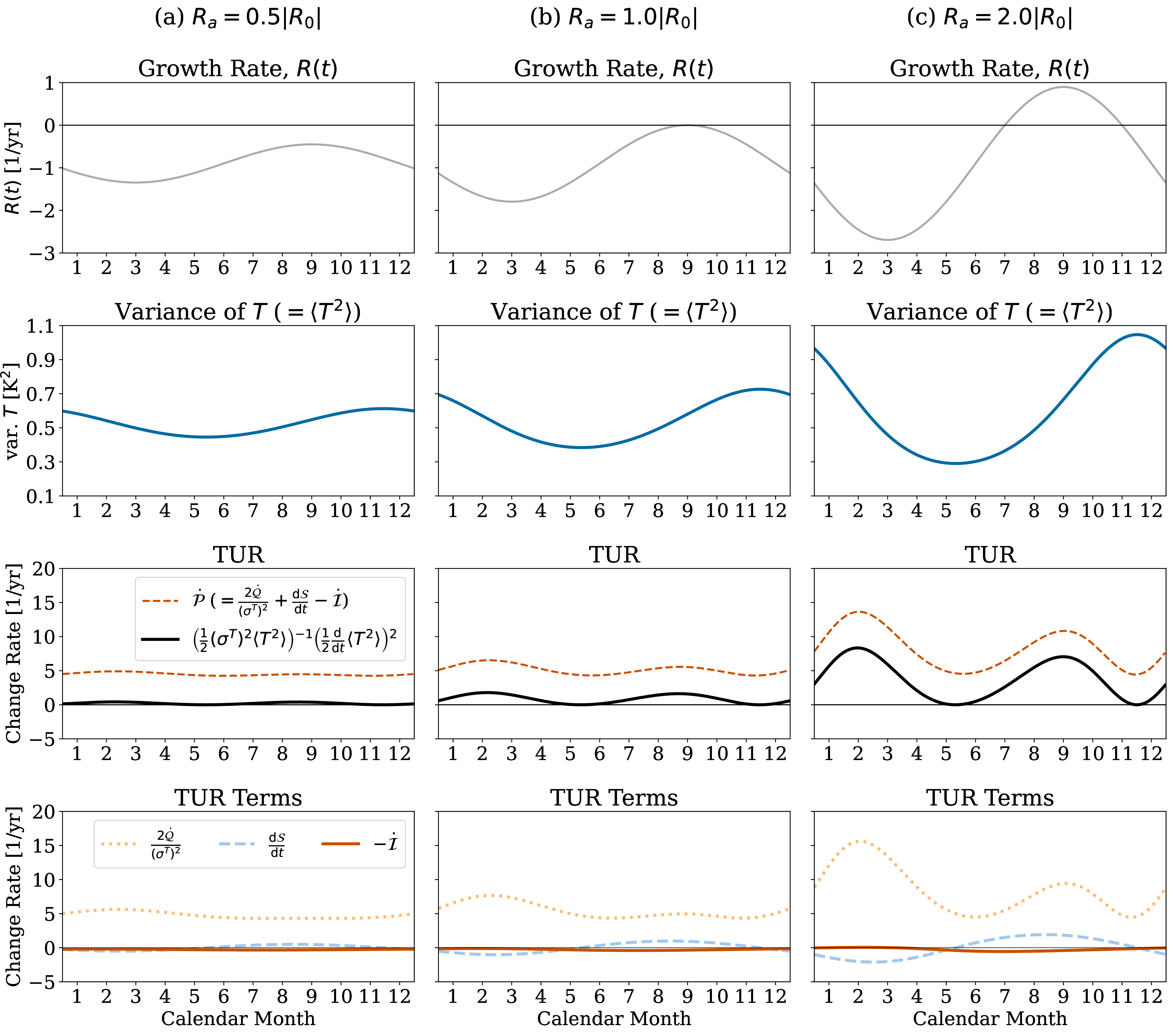
The TUR (17 ) means that net changes in \(\left\langle T^2 \right\rangle\), whether increases or decreases, are constrained by \(\dot{\cal P}\). Noise induces both net changes and fluctuations, which appear in the numerator and denominator of the right-hand side, respectively (Section [3]3.1). The rate \(\dot{\cal P}\) must be large enough to overcome the fluctuations and produce a net change; when it is insufficient, this constraint inhibits the net change. The minimum of \(\dot{\cal P}\) varies little with \(R_a\), whereas its maximum increases with \(R_a\) (Fig. 3a–c). Around September and February, \(\dot{\cal P}\) becomes large, relaxing the TUR constraint and permitting a net change in \(\left\langle T^2 \right\rangle\). The variance \(\left\langle T^2 \right\rangle\) then reaches its maximum around November, corresponding to the concentration of El Niño peaks (discussed in more detail below). Conversely, for small \(R_a\), the rate \(\dot{\cal P}\) is nearly uniform across seasons, and the seasonality of \(\left\langle T^2 \right\rangle\) is weak. In this case, fluctuations become dominant, and \(T\) can peak in any calendar month.
The leading term of \(\dot{\cal P}\), namely \({2\dot{\cal Q}}/{\left(\sigma^T\right)^2}\), peaks around September and February mainly because \(\lvert R(t) \rvert\) becomes large near these times: \(R(t)\) attains its maximum around September and its minimum around March (Fig. 1). Intuitively, when \(R(t)\) is minimal (that is, when it is most negative), \(R(t)T\) acts as damping of \(T\) in Eq. (1 ), increasing its irreversibility. Conversely, when \(R(t)\) is maximal, \(R(t)T\) acts as amplification of \(T\), also increasing its irreversibility. Both the minimum and the maximum of \(R(t)\) therefore correspond to maxima of irreversibility, together producing the wavenumber-2 structure of \({2\dot{\cal Q}}/{\left(\sigma^T\right)^2}\).
The next component of \(\dot{\cal P}\), the Shannon entropy tendency \({\rm d}{\cal S}/{\rm d}t\), diagnoses whether \(\left\langle T^2 \right\rangle\) is increasing or decreasing, because \({\cal S}\) is a monotonic function of \(\left\langle T^2 \right\rangle\) in the SRO by Gaussianity [49]. This sign information cannot be obtained from the TUR alone (Section [3]3.3). The entropy tendency peaks in August–September, when \(\left\langle T^2 \right\rangle\) is increasing; \({\cal S}\) itself then peaks in November–December, when \(\left\langle T^2 \right\rangle\) is large.
The final component of \(\dot{\cal P}\), the information flow \(\dot{{\cal I}}\) [Eq. (11 )], is the smallest and almost negligible. The information flow represents the change in the correlation between \(T\) and \(h\) induced by changes in \(T\) (Section [3]3.1). In the SRO, \(T\) and \(h\) fluctuate under noise but tend to be out of phase, with \(h\) leading \(T\) (Section 2). Although the correlation itself is strong, its tendency is small, likely keeping \(\dot{\cal I}\) small.
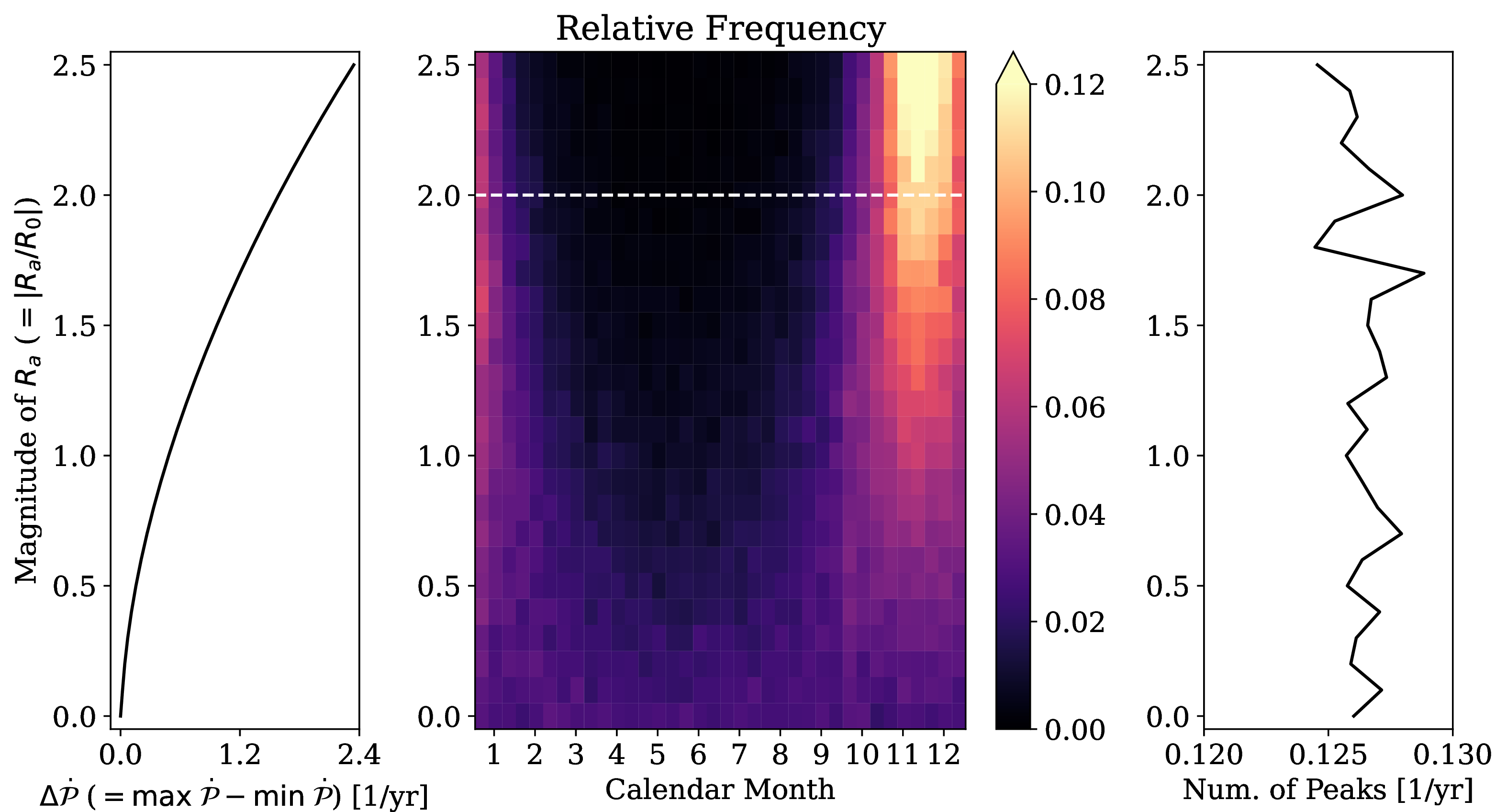
We next examine the calendar months in which El Niño peaks tend to occur in the SRO. We follow the procedure of . We varied \(R_a\) from 0 to \(2.5 \lvert R_0 \rvert\) and, for each value, integrated a single ensemble member for 50,000 years. For each time series, we computed the standard deviation of \(T\) and used it as the El Niño threshold. We then applied a 5-month running mean to \(T\) and defined an El Niño event as a time interval during which \(T\) continuously exceeds this threshold for at least 6 months. We extracted the local maxima of \(T\) within each event and counted them for each calendar month. Multiple maxima within a single event were counted separately if they were at least 5 months apart. The results are not sensitive to the integration length or running-mean window: similar peak distributions were obtained with a 10,000-yr integration, with different running-mean windows, and when only the global maximum of \(T\) in each event was counted.
Figure 4 shows the peak distributions. As \(R_a\) increases, the peaks become concentrated in November–December (middle panel), consistent with . The white horizontal dashed line marks \(R_a = 2.0 \lvert R_0 \rvert\), the value corresponding to observed ENSO . The number of peaks is approximately 0.125 per year (right panel) and is nearly independent of \(R_a\): their total changes little while their seasonal concentration strengthens. We characterize this concentration by the difference \(\Delta \dot{\cal P}\) (left panel), defined as \[\Delta \dot{\cal P} := \max \;\dot{\cal P} - \min \;\dot{\cal P}.\] Larger \(\Delta \dot{\cal P}\) corresponds to stronger seasonality of \(\left\langle T^2 \right\rangle\) and to stronger phase locking of El Niño in the SRO (Fig. 4, left). Thus, \(\Delta \dot{\cal P}\) is analogous to the seasonal energy index (SEI) of (Section 1) and serves as a phase-locking strength index.
In preparation for the climatological interpretation in Section [5]5.1, we discuss the cause of the wavenumber-2 structure based on the SRO expression for \({2\dot{\cal Q}}/{\left(\sigma^T\right)^2}\): \[\begin{align} \frac{2}{\left(\sigma^T\right)^2}\dot{\cal Q} &= \underbrace{\frac{2}{\left(\sigma^T\right)^2} R(t)^2 \left\langle T^2 \right\rangle}_{=A} + \underbrace{\frac{2}{\left(\sigma^T\right)^2} {2 R(t) F_1} \left\langle T h \right\rangle}_{=B} + \underbrace{\frac{2}{\left(\sigma^T\right)^2} \left(F_1\right)^2 \left\langle h^2 \right\rangle}_{=C} + \underbrace{R(t)}_{=D}.\label{eq:decompose-q-a-to-d} \end{align}\tag{18}\] See Appendix B for the derivation. The terms \(A\), \(B\), and \(C\) arise from expanding \(\langle \left[R(t) T+F_1 h\right]^2\rangle\). The remaining term \(D\) comes from the nonsmoothness of \(T\) and is introduced as a correction term through the Stratonovich product [25].
Figure 5 shows the time series of \(A\)–\(D\). As \(R_a\) increases, the seasonality of \(A\)–\(D\) strengthens, consistent with that of \({2\dot{\cal Q}}/{\left(\sigma^T\right)^2}\) (Fig. 3). The correction term \(D\) is not directly associated with physical processes; we therefore focus on \(A\), \(B\), and \(C\).
The seasonality of \({2\dot{\cal Q}}/{\left(\sigma^T\right)^2}\) is produced mainly by \(A\) and \(B\) [Eq. (18 )], whose relative contributions depend on the choice of \(h\). As in the preceding sections, we take \(h\) to represent the heat content over the entire equatorial Pacific (Section 2); the case of the western equatorial Pacific is discussed in Appendix C. The term \(A\) has a wavenumber-2 structure originating from \(R(t)^2\). The growth rate \(R(t)\) attains its extrema around September and March, with a larger absolute value in March, so \(A\) peaks in both seasons and is largest in late winter, although the precise timing and amplitude are modulated by the variance \(\langle T^2 \rangle\) (Fig. 5). The term \(B\) has a wavenumber-2 structure originating from the product \(R(t)\left\langle T h \right\rangle\): the covariance \(\left\langle T h \right\rangle\) is largest around August and smallest around early March, approximately in phase with \(R(t)\) (Figs. 1 and 2).
![Figure 5: Time series of the terms A, B, C, and D of the irreversibility indicator {2\dot{\cal Q}}/{\left(\sigma^T\right)^2} [Eq. (18 )]. (a) R_a = 0.5 \lvert R_0 \rvert, (b) R_a = 1.0 \lvert R_0 \rvert, and (c) R_a = 2.0 \lvert R_0 \rvert. In each panel, the black solid line shows the corresponding term (A, B, C, or D), and the orange dotted line shows {2\dot{\cal Q}}/{\left(\sigma^T\right)^2}. These terms were computed from the same simulation as in Fig. 3; see Appendix B for the derivation of Eq. (18 ).](/article/2606.19778/fig05.png "fig:")
We interpret the combined contribution \(A+B\) as the seasonal variation of irreversibility associated with air–sea interaction in the SRO: the growth rate \(R(t)\) includes the Bjerknes feedback (Section [5]5.1), and \(h\) and \(T\) interact through atmospheric processes such as wind stress [9], [10].
In the SRO, this air–sea irreversibility arises through a stochastic mechanism. The SRO is driven entirely by stochastic noise (Section 2). The growth rate \(R(t)\) acts as a “noise rectifier” that selectively amplifies or damps noise-driven fluctuations depending on the season. Although each ensemble member fluctuates randomly, an ensemble-wide seasonal bias toward increasing \(\left\langle T^2 \right\rangle\) emerges only through this rectification. A necessary condition for the emergence of this bias is an increase in the irreversibility indicator \(\dot{\cal Q}\).
Finally, the term \(C\) in \({2\dot{\cal Q}}/{\left(\sigma^T\right)^2}\) involves the variance \(\left\langle h^2 \right\rangle\) of the heat content [Eq. (18 )]. Although \(\left\langle h^2 \right\rangle\) itself peaks around May–June (Fig. 2), \(C\) contributes little to the seasonality of \({2\dot{\cal Q}}/{\left(\sigma^T\right)^2}\) (Fig. 5). Thus, a sufficient heat content alone does not guarantee the strong irreversibility required for rapid growth of \(\left\langle T^2 \right\rangle\). An energy-based perspective relies on heat content, whereas our entropy-based perspective focuses on irreversibility; these complementary viewpoints are discussed further in Section [5]5.1.
5 Discussion↩︎
5.1 Climatological interpretation↩︎
In Section 4, we showed that irreversibility in the SRO constrains the temporal evolution of SSTA variance and serves as an indicator of phase-locking strength. When the system is driven by noise, the realized SSTA time series are random. However, for \(\langle T^2 \rangle\) to increase or decrease in a given season, \(\dot{\cal P}\) [Eq. (8 )] must be large enough in that season. In the SRO, \(R(t)\) reaches its maximum and minimum around September and March, respectively; irreversibility (and hence \(\dot{\cal P}\)) peaks around these times.
The growth rate \(R(t)\) can be computed from climatology and characterizes how anomalies interact with the climatological background state. The temporal variation of \(R(t)T\) can be decomposed into multiple physical processes [9], [12], [15], [56]. To our knowledge, no consensus has yet been reached on which process is dominant, but the zonal advective feedback (ZA), for example, has been identified as a major term [15], [56]. ZA represents the advection of the climatological SST by anomalous zonal currents. If the anomalous zonal current is driven mainly by wind stress, ZA is attributed to the Bjerknes feedback. The seasonality of ZA has been linked to the seasonal variation of the air–sea coupling coefficient [15] and to the seasonal migration of the Intertropical Convergence Zone [56].
Within the SRO framework, the partial entropy production rate \(\dot{\cal P}\) depends on the climatology through the SRO coefficients and constrains the temporal variation of the SSTA variance. This is an entropic constraint: in general, entropy quantifies the possibility of any change, whereas energy is required to drive it. adopted an energetic perspective and showed that the seasonal energy index (SEI) peaks in boreal winter, providing the energy needed for the SSTA variance to grow. In contrast, we adopt an entropic perspective and find that \(\dot{\cal P}\) peaks in boreal autumn and late winter, relaxing the entropy bound on the tendency of \(\left\langle T^2 \right\rangle\). A definite seasonal change in \(\left\langle T^2 \right\rangle\) thus requires both sufficient available energy and a relaxed entropy constraint; the two perspectives are complementary but distinct. Indeed, \(\left\langle h^2 \right\rangle\), which corresponds to oceanic thermal energy, has only a small effect on \(\dot{\cal Q}\), the dominant term in \(\dot{\cal P}\) (Section 4).
Although energy and entropy are generally related, their connection in the SRO is not straightforward. In nonequilibrium physics, when the noise source is a heat bath, \(\dot{\cal Q}\) equals the energy dissipated as heat [22], [54]. It is unclear, however, whether the noise source of the SRO can be interpreted as a heat bath, so this dissipated-energy interpretation may not directly apply. At present, \(\dot{\cal Q}\) is understood as an indicator of irreversibility, given by the ratio of the forward and backward transition probabilities (Section [3]3.1). Even so, air–sea interaction typically involves dissipation [57], [58], and thus \(\dot{\cal Q}\) may also correspond to dissipated energy.
If \(\dot{\cal Q}\) were assumed to correspond to some kind of dissipated energy, then our results would be interpreted as follows (Fig. 6). In this case, \(\dot{\cal Q}\) would represent heat dissipated from the subsystem (the equatorial Pacific) to its environment (the rest of the climate system); the equatorial Pacific would then be energetically open. During the growth phase of ENSO, that is, when the variance \(\left\langle T^2 \right\rangle\) increases, the dissipation generated by irreversible motions would have to be exported from the equatorial Pacific. During the decay phase, when \(\left\langle T^2 \right\rangle\) decreases, an analogous export constraint would apply. However, energy is supplied to the subsystem during growth but released during decay, so the dissipation may differ between the two phases. This could underlie the asymmetry of \(\dot{\cal Q}\) between September and March (Fig. 3). Such export could proceed, for example, horizontally to the extratropics via teleconnections, to the other tropical basins (the Indian and Atlantic Oceans) via interbasin interactions, or vertically to space via atmospheric radiation. This dissipated-energy interpretation remains hypothetical, so a more realistic model is needed to test its validity and to further explore the physical connection between energy and entropy.
![Figure 6: Schematic of the irreversibility constraint on ENSO phase locking. In boreal summer (left), the SSTA distribution in the eastern Pacific is narrow, corresponding to small variance \left\langle T^2 \right\rangle. In boreal winter (right), the distribution broadens and \left\langle T^2 \right\rangle is large. For the variance to grow or decay between seasons, the TUR requires the irreversibility indicator \dot{\cal Q} (wavy arrows) to be sufficiently large. The SST climatology maps and SSTA histograms are computed from the CESM Large Ensemble [59], [60].](/article/2606.19778/fig06.png "fig:")
5.2 Future work↩︎
A natural first extension of the SRO toward a more realistic ENSO model is to incorporate nonlinear terms, state-dependent (multiplicative) noise, or red noise [17], [61]–[63]. TURs have also been formulated in broader stochastic settings that may be relevant to such extensions [40], [41], [64], [65]. Applying these results to the SRO, however, would require reformulating the variance of the current and the partial entropy production rate. Moreover, ENSO may be a noisy self-sustained oscillator rather than a damped one [18]; in that case, a TUR-like inequality could still constrain the coherence of the resulting stochastic limit cycle through its entropy production [66].
Another extension is to multivariable systems that include other ocean basins or atmospheric variables. For example, linear inverse models or extended ROs can capture the influence of interbasin interactions on ENSO [67], [68]. Full-system TURs have been obtained for multivariable systems [39], [41], but the subsystem TUR used in our study was derived only for the bivariate case [40], so further extension would be needed.
Finally, TURs hold for arbitrary high-dimensional systems [39], [41] and may apply to gridded ensemble data from general circulation models. This assumes that the resolved variables can be modeled as a Markov process. A practical challenge is that the entropy production rate requires the probability density function, which is difficult to estimate from finite ensemble data in high dimensions. The TUR can instead be used to estimate the entropy production rate from the mean and variance of a suitably chosen current [41]. These extensions would broaden the applicability of entropy-based constraints from idealized ROs to the full complexity of climate variability.
6 Conclusions↩︎
We analyzed the SRO using the TUR and showed that the SSTA variance, an indicator of phase-locking strength, is constrained by the partial entropy production rate \(\dot{\cal P}\). The dominant component of \(\dot{\cal P}\) is the irreversibility indicator \(\dot{\cal Q}\), given by the ratio of forward and backward transition probabilities of SSTA. The growth rate \(R(t)\) governs this irreversibility: \(R(t)\) reaches its maximum and minimum in boreal autumn and late winter, respectively, and \(\dot{\cal P}\) peaks at both times, relaxing the TUR constraint on the SSTA variance. As a result, the variance increases through boreal autumn, peaks in boreal winter, and then decreases toward late winter, corresponding to the observed seasonal concentration of SSTA peaks. Conversely, when irreversibility is insufficient, the TUR constraint prevents ENSO from growing or decaying.
We further provided a dissipated-energy interpretation for real ENSO. If \(\dot{\cal Q}\) were assumed to correspond to dissipated energy, the constraint on ENSO growth and decay would require this dissipation to be exported from the equatorial Pacific. Unlike standard settings in nonequilibrium physics, however, it is unclear whether the noise source of the SRO can be interpreted as a heat bath, so this interpretation remains hypothetical. A more realistic model is needed to test this hypothesis and to further explore the physical connection between entropy and dissipated energy.
Y. Yasuda was supported by Japan Society for the Promotion of Science (JSPS) KAKENHI (JP26K07197). T. Kohyama was supported by JSPS KAKENHI (JP23H01241, JP23K13169), the MEXT Program for the Advanced Studies of Climate Change Projection (SENTAN) (JPMXD0722680395), and the Sumitomo Foundation (Environmental Research Project).
The data and source code that support the findings of this study are preserved at the Zenodo repository (https://doi.org/10.5281/zenodo.20712622) and developed openly at the GitHub repository (https://github.com/YukiYasuda2718/enso_sro_stochastic_constraint).
We re-derive the instantaneous TUR of [40] using the short-time-limit method of [41]. We first set up the problem and then introduce the second law of information thermodynamics [46], [50] (Appendix A6.1). By applying the Cauchy–Schwarz inequality to this second law, we obtain the TUR based on a general weight function \(g(T,h)\) (Appendix A6.2). We then derive the TUR for the case \(g(T,h) = T\) (Appendix A6.3). We finally show that \(\dot{\cal Q}\) is given by the ratio of the forward and backward transition probabilities (Appendix A6.4).
6.1 Second law of information thermodynamics↩︎
We consider the following bivariate stochastic differential equation (SDE): \[\begin{align} {\rm d} T &= -a^T(T, h, t) {\rm d} t + \sigma^T {\rm d} W^T, \tag{19}\\ {\rm d} h &= -a^h(T, h, t) {\rm d} t + \sigma^h {\rm d} W^h. \tag{20} \end{align}\] As in the SRO, \(T\) and \(h\) denote the sea surface temperature anomaly and thermocline depth anomaly, respectively. The quantities \(a^T\) and \(a^h\) are nonlinear functions that may explicitly depend on \(t\), and \(W^T\) and \(W^h\) are mutually independent standard Wiener processes. They are related to the Gaussian white noises \(\xi^T\) and \(\xi^h\) by \({\rm d} W^T = \xi^T {\rm d}t\) and \({\rm d} W^h = \xi^h {\rm d}t\). This system includes the linear SRO [Eqs. (1 )–(5 )] as a special case: for example, setting \(-a^T = R(t) T + F_1 h\) recovers Eq. (1 ). The TUR holds independently of the specific form of the drift, and thus we consider a general nonlinear SDE here. We assume additive noise (that is, \(\sigma^T\) and \(\sigma^h\) are constants), as in the SRO analyzed in this study. TURs can also be formulated in broader Langevin settings [40], [41], but multiplicative noise would require re-deriving the probability flux, current variance, and explicit partial-entropy-production terms.
For this SDE, the joint probability density function \(p^{T,h}\) of the state variables \((T,h)\) obeys the Fokker–Planck equation [42]: \[\begin{align} \frac{\partial p^{T,h}}{\partial t} &= -\frac{\partial J^T}{\partial T} -\frac{\partial J^h}{\partial h}, \\ p^{T,h} &:= p(T,h,t), \\ J^T &:= -a^T p^{T,h}-\frac{\left(\sigma^T\right)^2}{2} \frac{\partial p^{T,h}}{\partial {T}},\tag{21} \\ J^h &:= -a^h p^{T,h}-\frac{\left(\sigma^h\right)^2}{2} \frac{\partial p^{T,h}}{\partial {h}}.\tag{22} \end{align}\] This is a continuity equation in the \((T,h)\) state space: the time derivative of \(p^{T,h}\) equals minus the divergence of the probability flux \((J^T, J^h)\). In the main text, we write \(p^{T,h}\) as \(p_t(T_t, h_t)\) [e.g., Eq. (12 )]. When the coefficients of the SDE explicitly depend on \(t\) (for example, \(R(t)\) in the SRO), \(p^{T,h}\) can also explicitly depend on \(t\); the subscript \(t\) in \(p_t\) expresses this time dependence. We impose the boundary condition that the probability flux vanishes at infinity in the \((T,h)\) state space. In what follows, we derive the TUR for \(T\); analogous formulas hold for \(h\).
The following inequality, the second law of information thermodynamics, holds for \(T\) [46], [50]. For a detailed review, see [28]. Although that review assumes that \(a^T\) and \(a^h\) do not explicitly depend on \(t\), this assumption is not used in the derivation, so the same argument extends to time-dependent \(a^T\) and \(a^h\): \[\begin{align} \dot{{\cal P}} := \frac{2\dot{\cal Q}}{\left(\sigma^T\right)^2}+\frac{{\rm d} {\cal S}}{{\rm d} t}-\dot{{\cal I}}&=\left\langle\frac{2J^T}{p^{T,h} \left(\sigma^T\right)^2} \circ \frac{{\rm d} T}{{\rm d} t}\right\rangle=\int {\rm d}T{\rm d}h \; \frac{2\left(J^T\right)^2}{p^{T,h} \left(\sigma^T\right)^2} \geq 0. \label{eq:second-law-in-app} \end{align}\tag{23}\] The quantity \(\dot{{\cal P}}\) is called the partial entropy production rate and is always nonnegative [43]–[45]. Equality holds when \(J^T = 0\), that is, when the probability flux associated with the \(T\) transitions vanishes (zero partial entropy production) [50]. The quantities in the inequality are defined as follows: \[\begin{align} \dot{\cal Q}&:=\left\langle -a^T \circ \frac{{\rm d} T}{{\rm d} t}\right\rangle, \tag{24} \\ {\cal S} &:=-\int {\rm d} T \; p(T,t) \ln p(T,t), \\ p(T,t) &:=\int {\rm d}h \; p(T, h, t), \\ \dot{{\cal I}} &:= \int {\rm d}T{\rm d}h \; \frac{\partial J^T}{\partial T} \ln \left[ \frac{p(T,t)}{p(T,h,t)}\right]. \tag{25} \end{align}\] The quantity \(\dot{\cal Q}\) is an indicator of irreversibility [21], [47], [48], [54] and is further discussed in Appendix A6.4. The Shannon entropy \({\cal S}\) represents the uncertainty of the continuous variable \(T\), that is, a differential entropy [49]. In the main text, we write \(p(T,t)\) as \(p_t(T_t)\) [e.g., Eq. (10 )]. The quantity \(\dot{{\cal I}}\) is called the information flow from \(h\) to \(T\) and represents the contribution to the rate of change of the correlation between \(T\) and \(h\) induced by the time evolution of \(T\) [43], [45], [46], [50]. It is not the total time derivative of their mutual information, because that total tendency also includes the contribution induced by the time evolution of \(h\). Equation (11 ) may seem more intuitive, but Eq. (25 ) is more general because it also holds for multivariable systems [50].
6.2 TUR based on a general weight function \(g(T,h)\)↩︎
We derive the TUR for the following current \({\cal J}\) based on a general weight function: \[\begin{align} {\cal J} &:= g(T,h) \circ {\rm d}T \\ &= \left[ -a^T g + \frac{\left(\sigma^T\right)^2}{2} \frac{\partial g}{\partial T} \right] {\rm d} t + g \sigma^T {\rm d} W^T, \end{align}\] where we substitute the definition of the Stratonovich product, perform a Taylor expansion, and neglect terms of higher order in \({\rm d}t\). The mean of the current then becomes [41]: \[\begin{align} \left \langle {\cal J} \right \rangle &= {\rm d} t \left \langle -a^T g + \frac{\left(\sigma^T\right)^2}{2} \frac{\partial g}{\partial T} \right \rangle \\ &= {\rm d} t \int {\rm d}T{\rm d}h \; \left[ -a^T g + \frac{\left(\sigma^T\right)^2}{2} \frac{\partial g}{\partial T} \right] p^{T,h} \\ &= {\rm d} t \int {\rm d}T{\rm d}h \; gJ^T. \end{align}\] The last equality follows by integration by parts, expressing the result in terms of the probability flux \(J^T\) [Eq. (21 )]. Next, the variance of the current becomes [41]: \[\begin{align} {\rm Var}[{\cal J}] &:= \left \langle {\cal J}^2 \right \rangle - \left \langle {\cal J} \right \rangle^2 \\ &= \left \langle {\cal J}^2 \right \rangle + O\left(\left({\rm d}t\right)^2\right) \\ &= {\rm d} t \left[\int {\rm d}T{\rm d}h \; \left(\sigma^T\right)^2 g^2 p^{T,h}\right]. \end{align}\] Here, we use \(({\rm d} W^T)^2 = {\rm d}t\) [42] and neglect terms of second order or higher in \({\rm d}t\).
With these preparations, the TUR follows by applying the Cauchy–Schwarz inequality [41]: \[\begin{align} {\rm Var}[{\cal J}] \dot{\cal P} \; {\rm d} t &= ({\rm d} t)^2 \left( \int {\rm d}T{\rm d}h \; \left(\sigma^T\right)^2 g^2 p^{T,h} \right) \left( \int {\rm d}T{\rm d}h \; \frac{2\left(J^T\right)^2}{p^{T,h} \left(\sigma^T\right)^2} \right) \\ &\ge ({\rm d} t)^2 \left( \int {\rm d}T{\rm d}h \; \cancel{\sigma^T} \; g \; \cancel{\sqrt{p^{T,h}}} \frac{\sqrt{2}J^T}{\cancel{\sqrt{p^{T,h}}}\;\cancel{\sigma^T}} \right)^2 \\ &= 2\left \langle {\cal J} \right \rangle^2. \end{align}\] Assuming \({\rm Var}[{\cal J}] > 0\), we obtain the following TUR [40]: \[\begin{align} \frac{\dot{\cal P}}{2} \ge \frac{\left \langle {\cal J} \right \rangle^2}{{\rm Var}[{\cal J}] \; {\rm d} t}. \label{eq:tur-in-appendix} \end{align}\tag{26}\] The right-hand side is the squared mean of the current normalized by the variance, corresponding to a signal-to-noise ratio. If this ratio is regarded as a measure of precision, then the TUR can be interpreted as stating that increasing precision requires paying the thermodynamic cost of increasing the partial entropy production rate \(\dot{\cal P}\). For the full system \((T,h)\), a TUR can be derived in the same way [41], but a characteristic feature of the subsystem TUR for \(T\), Eq. (26 ), is that \(\dot{\cal P}\) contains the information flow \(\dot{\cal I}\). This means that information transfer from \(h\) to \(T\) can modify the upper bound on the precision [40].
6.3 TUR based on the specific weight function \(g(T,h)=T\)↩︎
We derive the TUR for the case in which the weight function is \(g(T,h)=T\). First, the mean and variance of the current \({\cal J}\) become: \[\begin{align} \left \langle {\cal J} \right \rangle &= \left\langle T \circ {\rm d} T \right\rangle = \frac{1}{2} \left\langle {\rm d}(T^2) \right\rangle = \frac{1}{2} \left\langle \frac{{\rm d} T^2}{{\rm d}t} \right\rangle {\rm d}t = \frac{1}{2} \left( \frac{{\rm d}}{{\rm d}t} \left\langle T^2 \right\rangle \right) {\rm d}t, \tag{27} \\ {\rm Var}[{\cal J}] &= \left[\int {\rm d}T{\rm d}h \; \left(\sigma^T\right)^2 T^2 p^{T,h}\right] {\rm d}t = \left(\sigma^T\right)^2\left\langle T^2 \right\rangle {\rm d}t.\tag{28} \end{align}\] In Eq. (27 ), we use the fact that the Stratonovich product satisfies the chain rule of differentiation [42]. In general, the current \({\cal J}\) represents a net displacement, but by using \(T\) as the weight function, its mean \(\left \langle {\cal J} \right \rangle\) becomes the net change in \(\left\langle T^2 \right\rangle\). Positive and negative changes are both possible, and the sign corresponds to the direction of the current. In Eq. (28 ), the variance of the current, \({\rm Var}[{\cal J}]\), involves the squared noise amplitude \(\left(\sigma^T\right)^2\) and the mean square of \(T\).
Thus, the TUR becomes the following inequality: \[\begin{align} \frac{\dot{\cal P}}{2} \ge \frac{1}{\left(\sigma^T\right)^2\left\langle T^2 \right\rangle} \left( \frac{1}{2} \frac{{\rm d}}{{\rm d}t} \left\langle T^2 \right\rangle \right)^2. \end{align}\] The partial entropy production rate \(\dot{\cal P}\) provides an upper bound on the normalized squared tendency of \(\left\langle T^2 \right\rangle\). After this normalization, a large tendency of \(\left\langle T^2 \right\rangle\) must be accompanied by a sufficiently large \(\dot{\cal P}\). In this derivation, we neither use the specific form of the SRO’s governing equations nor assume any specific initial condition. The derived TUR holds at any time, for any initial condition, and for any \(T\) obeying an arbitrary nonlinear SDE with additive noise, provided that the current variance is nonzero. For the specific current used here, this condition requires \(\sigma^T>0\) and \(\left\langle T^2 \right\rangle>0\).
6.4 \(\dot{\cal Q}\) as a ratio of transition probabilities↩︎
We show that \(\dot{\cal Q}\) is given by a ratio of transition probabilities [22], [48], [54]. First, the probability density function of \({\rm d} W^T\) is a Gaussian [25]: \[p({\rm d} W^T) = \frac{1}{\sqrt{2\pi {\rm d}t}} \exp\left\{ -\frac{1}{2} \frac{\left({\rm d} W^T\right)^2}{{\rm d}t} \right\}.\] This expression holds for an infinitesimal increment \({\rm d} W^T\) at any time. Suppose that the state at time \(t\) is \((T_t, h_t)\). By discretizing the governing equation (19 ) for \(T\) using the Euler–Maruyama method and solving for \({\rm d} W^T\), we obtain the transition density of \(T\) from \(p({\rm d} W^T)\). The noise coefficient matrix in the governing equations [Eqs. (19 ) and (20 )] is diagonal, and thus the noise \({\rm d} W^T\) contributes only to the transition of \(T\) [46]: \[\begin{align} p_t(T_{t+{\rm d}t} \mid T_t, h_t) = \frac{1}{\sqrt{2\pi \left(\sigma^T\right)^2 {\rm d}t}} \exp\left\{-\frac{1}{2} \frac{\left[T_{t+{\rm d}t} - T_t + a^T(T_t, h_t, t){\rm d}t\right]^2}{\left(\sigma^T\right)^2{\rm d}t}\right\}. \end{align}\] Here, we set \({\rm d} T = T_{t+{\rm d}t} - T_t\) and use the fact that the Jacobian of the variable transformation is \(1/\sigma^T\). When \(a^T\) explicitly depends on \(t\), \(p_t\) also explicitly depends on \(t\). We next consider the backward transition. The variable \(T\) does not change sign under time reversal, and thus the backward transition density is given by \[\begin{align} p_t(T_t \mid T_{t+{\rm d}t}, h_t) = \frac{1}{\sqrt{2\pi \left(\sigma^T\right)^2 {\rm d}t}} \exp\left\{-\frac{1}{2} \frac{\left[T_t - T_{t+{\rm d}t} + a^T(T_{t+{\rm d}t}, h_t, t){\rm d}t\right]^2}{\left(\sigma^T\right)^2{\rm d}t}\right\}. \end{align}\]
Taking the logarithm of the ratio of the forward and backward transition densities yields: \[\begin{align} \ln \frac{p_t(T_{t+{\rm d}t} \mid T_t, h_t)}{p_t(T_t \mid T_{t+{\rm d}t}, h_t)} &= -\frac{2}{\left(\sigma^T\right)^2}\frac{a^T(T_t, h_t, t) + a^T(T_{t+{\rm d}t}, h_t, t)}{2} \left( T_{t+{\rm d}t} - T_t \right) + O({\rm d}t) \\ &= -\frac{2}{\left(\sigma^T\right)^2}\frac{a^T(T_t, h_t, t) + a^T(T_{t+{\rm d}t}, h_{t+{\rm d}t}, t+{\rm d}t)}{2} \left( T_{t+{\rm d}t} - T_t \right) + O({\rm d}t) \\ &= - \frac{2}{\left(\sigma^T\right)^2} a^T(T_t, h_t, t) \circ {\rm d}T + O({\rm d}t). \end{align}\] Taking the ensemble average and using the definition of \(\dot{\cal Q}\) [Eq. (24 )], we obtain [22], [48], [54]: \[\begin{align} \left\langle \ln \frac{p_t(T_{t+{\rm d}t} \mid T_t, h_t)}{p_t(T_t \mid T_{t+{\rm d}t}, h_t)} \right\rangle &= \frac{2}{\left(\sigma^T\right)^2} \dot{\cal Q} {\rm d}t. \end{align}\] The neglected \(O({\rm d}t)\) term becomes \(o({\rm d}t)\) through the ensemble average and thus does not contribute to \(\dot{\cal Q}\). The quantity \(\dot{\cal Q}\) is proportional to the logarithm of the ratio of the forward and backward transition probabilities. The more likely the forward transition is relative to the backward transition (that is, the more irreversible the transition), the larger \(\dot{\cal Q}\). When the noise source is a heat bath in equilibrium, \(\dot{\cal Q}\) equals the heat per unit time dissipated from the system to the bath [22], [48], [54]. However, when the noise source is not a heat bath (i.e., noise is not thermal), it is not clear whether \(\dot{\cal Q}\) can be interpreted as heat. In Section [5]5.1, we discuss the interpretation of \(\dot{\cal Q}\) for real ENSO.
This appendix presents the expressions for the stochastic-thermodynamic quantities based on the SRO’s governing equations [Eqs. (1 )–(5 )]. For general bivariate linear SDEs with time-dependent coefficients, these quantities were derived by [51] and [52]. Here, we present only those used in this study.
The stochastic-thermodynamic quantities (e.g., \(\dot{\cal Q}\)) are given by the means and covariance matrix of \(T\) and \(h\). We therefore discuss the time evolution of these statistical quantities. The evolution equations for the means are obtained by taking the ensemble average of the SRO [Eqs. (1 ) and (2 )]: \[\begin{align} \frac{{\rm d}\left\langle T \right\rangle}{{\rm d} t}&=R(t) \left\langle T \right\rangle +F_1 \left\langle h \right\rangle, \\ \frac{{\rm d}\left\langle h \right\rangle}{{\rm d} t}&=-\varepsilon \left\langle h\right\rangle -F_2 \left\langle T \right\rangle. \end{align}\] The means at each time \(t\) are obtained by numerically solving these equations. Since the SRO is a damped oscillator (Section 2), the means relax to zero. Next, we denote the covariance matrix by \(\mathsf{\Sigma}\): \[\mathsf{\Sigma} :=\left( \begin{array}{cc} \Sigma^{TT} & \Sigma^{Th} \\ \Sigma^{hT} & \Sigma^{hh} \end{array} \right),\] where \(\Sigma^{Th}=\Sigma^{hT}\). Using the linearity of the SRO, the time evolution of \(\mathsf{\Sigma}\) is given by [42], [52]: \[\begin{align} \frac{{\rm d} \mathsf{\Sigma}}{{\rm d} t} &= -\mathsf{A}\mathsf{\Sigma} - \mathsf{\Sigma}\mathsf{A}^{\rm T} + \mathsf{B}, \\ \mathsf{A} &:= \left( \begin{array}{cc} -R(t) & -F_1 \\ F_2 & \varepsilon \end{array} \right), \\ \mathsf{B} &:= \left( \begin{array}{cc} \left(\sigma^{T}\right)^2 & 0 \\ 0 & \left(\sigma^h\right)^2 \end{array} \right). \end{align}\] The covariance matrix at each time \(t\) is obtained by numerically solving these equations. For Figs. 3, 5, and 8, we integrated the mean and covariance equations with the explicit Euler method using a time step of \(1/360\) yr for 200 yr. The initial mean was \(\left(\langle T\rangle,\langle h\rangle\right)=(0~{\rm K},10~{\rm m})\). The initial covariance matrix was the steady covariance matrix obtained by fixing the coefficients at the initial time. We then used the last 360 time steps as the final model year.
After spin-up, this covariance matrix determines the covariance-only expressions for the stochastic-thermodynamic quantities used in the TUR. This reduction assumes that \((T,h)\) is in the cyclostationary Gaussian state reached by the linear additive-noise SRO after the effect of the initial condition has decayed [42]. The resulting expressions are [51], [52]: \[\begin{align} \dot{\cal Q} &= -\left\langle a^T \circ \frac{{\rm d} T}{{\rm d} t}\right\rangle \\ &= \left\langle (a^T)^2 \right\rangle - \left\langle \frac{\partial a^T}{\partial T} \right\rangle \frac{\left(\sigma^T\right)^2}{2} \\ &= R(t)^2 \left\langle T^2 \right\rangle + 2 R(t) F_1 \left\langle T h \right\rangle + \left(F_1\right)^2 \left\langle h^2 \right\rangle + \frac{R(t)\left(\sigma^T\right)^2}{2}, \\ \frac{{\rm d} {\cal S}}{{\rm d} t} &= \frac{1}{2\Sigma^{TT}} \frac{{\rm d} \Sigma^{TT}}{{\rm d} t} \\ &= R(t) + \frac{F_1\Sigma^{Th}}{\Sigma^{TT}} + \frac{\left(\sigma^T\right)^2}{2\Sigma^{TT}}, \\ \dot{{\cal I}} &= \frac{F_1\Sigma^{Th}}{\Sigma^{TT}} - \frac{\left(\sigma^T\right)^2 \Sigma^{hh}}{2\det \mathsf{\Sigma}} + \frac{\left(\sigma^T\right)^2}{2\Sigma^{TT}}. \end{align}\] In the above expressions, the explicit time dependence is written only for the growth rate \(R(t)\), but the means and covariance matrix also depend on \(t\). These quantities (\(\dot{\cal Q}\), \({\rm d}{\cal S}/{\rm d}t\), and \(\dot{{\cal I}}\)) yield the partial entropy production rate \(\dot{\cal P}\) via Eq. (23 ), and the TUR (26 ) can then be evaluated.
We discuss the results obtained with the parameter set of [17], in which \(h\) is taken as the thermocline depth anomaly in the western equatorial Pacific. In the main text, following , \(h\) is taken as the thermocline depth anomaly over the entire equatorial Pacific. Here, we show only the figures that differ qualitatively from those in the main text.
Figure 7 shows the simulation results of the SRO. The main difference from Fig. 2 is the sign of the covariance \(\left\langle T h \right\rangle\), which is always negative regardless of the time dependence of \(R\). Note that the phase structure of the covariance itself is similar when \(R(t)\) varies in time: it reaches a maximum toward summer. This negative covariance reflects a statistical tendency of the trajectory in the state space \((T,h)\) [17]. The trajectory \((T_t, h_t)\) tends to have a negative slope when \(h\) is taken as the thermocline depth anomaly in the western equatorial Pacific, but a positive slope when taken over the entire equatorial Pacific. See [17] for details.
![Figure 7: Simulation results of the SRO with the parameter set of [17], where h is the thermocline depth anomaly in the western equatorial Pacific. (a) Steady SRO with R_a = 0. (b) Unsteady SRO with R_a = 5.3 \lvert R_0 \rvert. All other settings are the same as in Fig. 2.](/article/2606.19778/fig07.png "fig:")
Figure 8 shows the time series of \(A\)–\(D\) composing \({2\dot{\cal Q}}/{\left(\sigma^T\right)^2}\) [Eq. (18 )]. As in Fig. 5, \({2\dot{\cal Q}}/{\left(\sigma^T\right)^2}\) exhibits a wavenumber-2 structure. We again focus on \(A\)–\(C\). First, \(C\) involves the thermocline-depth variance \(\left\langle h^2 \right\rangle\), but its seasonality is weak. This result suggests that the magnitude of \(\left\langle h^2 \right\rangle\) does not necessarily correspond to the magnitude of irreversibility.
As in Fig. 5, the seasonality of \({2\dot{\cal Q}}/{\left(\sigma^T\right)^2}\) is produced mainly by \(A\) and \(B\), but their relative contributions differ. The term \(A\) has a wavenumber-2 structure originating from \(R(t)^2\). The growth rate \(R(t)\) attains its extrema around September and March, so \(A\) peaks in both seasons, although the precise timing and amplitude are modulated by the variance \(\langle T^2 \rangle\). By contrast, the term \(B\) has a wavenumber-1 structure, unlike its wavenumber-2 structure in Fig. 5. The covariance \(\left\langle T h \right\rangle\) is always negative; thus, \(B\) varies as \(-R(t)\) [Eq. (18 )]. The physical picture of ENSO should not depend on the choice of variables; therefore, the difference between Figs. 5 and 8 suggests that \(A\) and \(B\) should not be interpreted separately. The combined contribution \(A+B\) represents the seasonal variation of irreversibility associated with air–sea interaction in the SRO.
![Figure 8: Time series of the terms A, B, C, and D of the irreversibility indicator {2\dot{\cal Q}}/{\left(\sigma^T\right)^2} [Eq. (18 )] with the parameter set of [17], where h is the thermocline depth anomaly in the western equatorial Pacific. (a) R_a = 1.0 \lvert R_0 \rvert, (b) R_a = 3.0 \lvert R_0 \rvert, and (c) R_a = 6.0 \lvert R_0 \rvert. The amplitudes increase from (a) to (c); the largest case, R_a = 6.0 \lvert R_0 \rvert, is close to the actual H26 ratio R_a \simeq 5.3 \lvert R_0 \rvert used in Fig. 7. All other settings are the same as in Fig. 5.](/article/2606.19778/fig08.png "fig:")