A Flat Connection:
The Pooling Factor and the Geometry of Centring in Hierarchical MCMC1
June 17, 2026
Abstract
Standard MCMC diagnostics (\(\hat{R}\), effective sample size, divergence counts) detect whether a chain has mixed, but not why it has not. We ask whether the centring/non-centring obstruction in hierarchical models has
a geometric cause beyond the metric. The joint parameter space is a fiber bundle (hyperparameters the base, group-level parameters the fibers), and the Fisher information metric induces an Ehresmann connection \(A =
-G_{FF}^{-1}G_{BF}\); the natural hypothesis is that the obstruction is its curvature, felt by the sampler as holonomy. We prove this false. The connection is flat for any smooth hierarchical posterior, not only the Gaussian or
conjugate case, because its horizontal leaves are the level sets of the fiber score \(\partial_{\boldsymbol{\alpha}}\log p\): there is no geometric obstruction above the metric. What remains is statistical, not geometric,
and the flat connection identifies it as a single quantity: the conditional dependence of fiber on base, governed per group by the prior fraction \(\pi_j\), the classical pooling factor. From it the framework
recovers the established picture, that the prior-dominated groups are the ones that mix slowly and that the optimal per-group non-centring weight follows in closed form, and a simulation study then separates this base–fiber coupling from the funnel, a
distinct base-space pathology, by their opposite dependence on the hierarchical variance. A direct attribution test confirms that NUTS does not transport the fiber: the chain-level footprint is excess conditional autocorrelation in prior-dominated groups,
exactly as \(\pi_j\) predicts. Genuine, even rotational, curvature does appear — but only for connections built from a sampler’s working metric (a fixed mass matrix), where holonomy re-enters as an
algorithmic rather than geometric phenomenon. The prior-fraction diagnostic is distributed as the open-source R package fibr, with the geometric methods as accompanying reproduction code.
Keywords: Markov chain Monte Carlo, hierarchical models, fiber bundles, Ehresmann connection, flat connection, holonomy, prior fraction, pooling factor, centering, convergence diagnostics.
1 Introduction↩︎
A central challenge in Bayesian computation is the hierarchical model. The joint parameter space of a two-level model \(-\) hyperparameters \((\mu, \sigma)\) and group-level parameters \((\alpha_1, \ldots, \alpha_J)\) \(-\) has a geometry that makes it simultaneously natural to write and difficult to sample from. The pathology is well documented: the centred parameterisation develops a funnel, non-centred parameterisations help when the prior dominates, and the right choice depends on a balance of prior and likelihood information that varies by group and dataset.
A geometric account of this trade-off already exists, at the level of the metric. [1] anatomised the funnel and showed that the optimal parameterisation is governed by the relative contribution of prior and likelihood to a group’s posterior (centred when the likelihood dominates, non-centred when the prior does) and [2] characterised the centred/non-centred trade-off in the same terms. [3] sharpened this into an equivalence: an incomplete reparameterisation such as centering versus non-centering is equivalent to modifying the Riemannian metric directly, so the two parameterisations are mirror-image metric geometries rather than genuinely different targets. At the metric level, then, the obstruction is well understood.
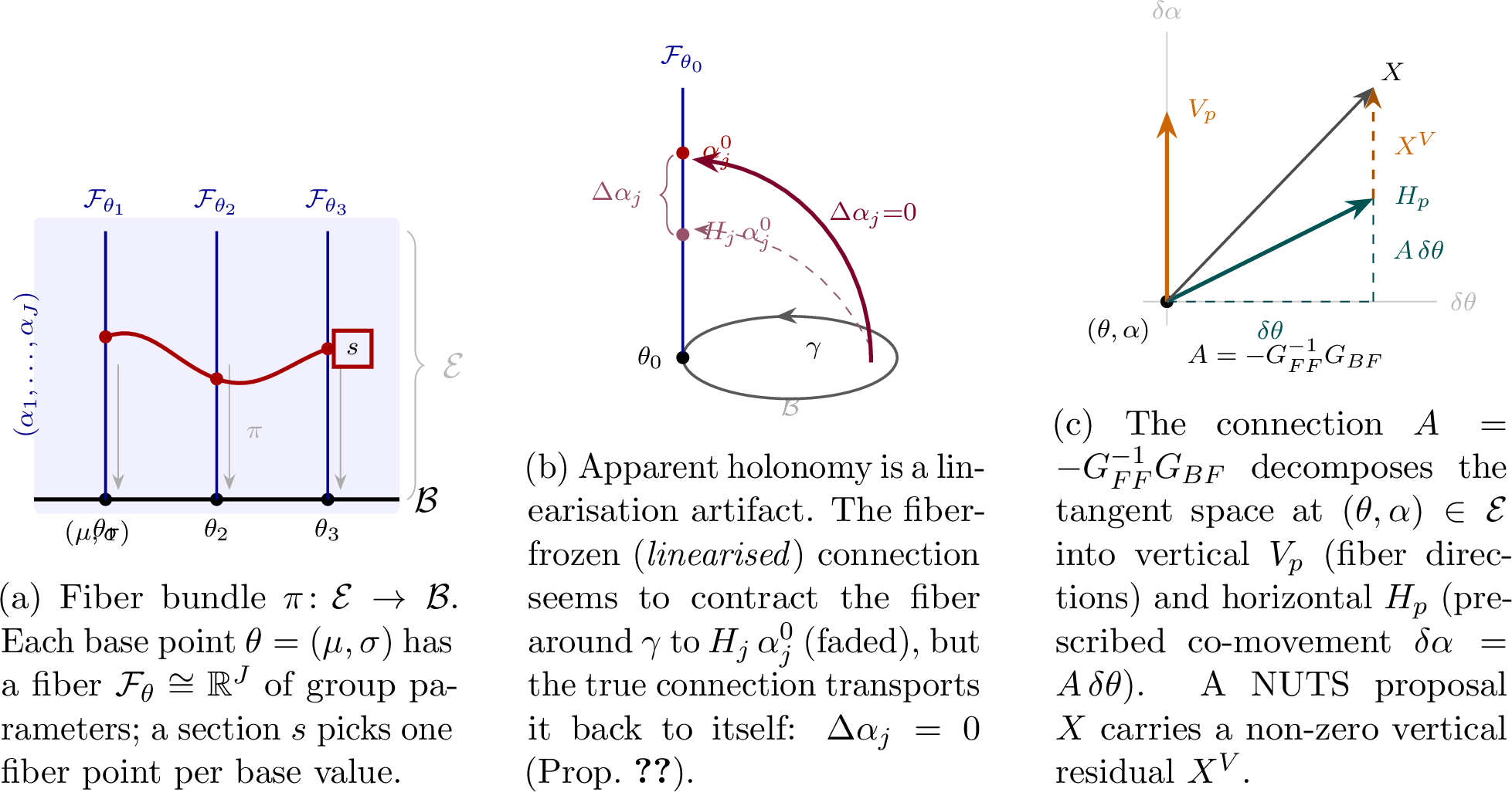
What is not yet settled is whether there is structure beyond the metric. The base–fiber split of the joint space is a fiber bundle, and a metric on the total space induces not only a Riemannian geometry but a connection, a rule for how the fiber must co-move with the base as the hyperparameters change. A natural hypothesis, which we state here as our own, since to our knowledge it does not appear in the statistics literature, is that the residual obstruction is the curvature of this connection, carried into the chain as holonomy: a net contraction of the fiber after the hyperparameters traverse a closed loop (Figure 1). Were it true, this would be a connection-level account sitting above the metric-level one, and it would tell the sampler something the metric does not: that closed excursions in \((\mu,\sigma)\) leave a systematic, transportable imprint on the group parameters.
This hypothesis belongs to the geometric program in MCMC, and it is that program the proof is aimed at. Riemannian-manifold HMC [4] and the differential-geometric account of Hamiltonian flow [5], [6] navigate hierarchical posteriors by exploiting the curvature of the Fisher metric, while a parallel line learns reparameterising transformations that absorb the funnel automatically [7]. A connection-curvature account of centering would slot directly into this program: it would licence samplers that parallel-transport the fiber as the hyperparameters move, rather than only reparameterise, and would motivate proposals built from the connection. Whether that structure exists is therefore worth settling before such a method is built.
Our central finding is that this hypothesis is false, and not just for the canonical model. The object is the metric-orthogonal Ehresmann connection \(A= -G_{FF}^{-1}G_{BF}\), the horizontal distribution \(G\)-orthogonal to the fibers, and we prove it is flat for any smooth hierarchical posterior (Proposition 1): its horizontal leaves are the level sets of the fiber score \(\partial_{\boldsymbol{\alpha}}\log p\), so a global flat trivialisation always exists and there is no holonomy to obstruct mixing. Gaussianity, conjugacy, and the dimension of the fiber are irrelevant; the logistic GLMM (Proposition 4) is one closed-form instance. The connection-level account collapses onto the metric-level one. What survives is not geometric but statistical: the conditional dependence of the fiber on the base, governed per group by the prior fraction \(\pi_j\), the pooling factor of [8], the precise form of the prior/likelihood balance whose role [1] established geometrically, which the bundle geometry now produces in closed form, and which, once the connection is known to be flat, is the only thing left governing the obstruction. The Fisher information actually carries several connections, of which only this one is at issue; we keep them apart in Section 3.4. The geometry is not thereby vacuous, however: genuine, even rotational, curvature reappears as soon as one transports along a sampler’s working metric rather than the true Hessian, and that is where holonomy returns — as an algorithmic rather than a geometric phenomenon (Section 9.2).
Standard diagnostics do not identify this mechanism. \(\hat{R}\) [9], [10] measures chain-to-chain variability. ESS measures autocorrelation. Divergence counts flag regions of high curvature in the Hamiltonian, not in the parameter-space geometry. All of these register the symptoms of the obstruction (slow mixing in the affected coordinates), but none localises the base–fiber coupling to specific groups, and none indicates the remedy (which groups to reparameterise). The empirical sections show that the mechanism’s chain-level signature is structured conditional autocorrelation localised in prior-dominated groups and predicted by the analytic prior fraction \(\pi_j\), rather than transport-following drift — consistent with the connection being flat.
1.1 Contributions↩︎
This paper makes the following contributions.
Geometric framework and a universal flatness theorem (Section 3). We formalise the fiber bundle structure of hierarchical posterior parameter spaces, on which the Fisher information metric induces a natural Ehresmann connection \(A = -G_{FF}^{-1}G_{BF}\). Our main geometric result (Proposition 1) is that this connection is flat for any smooth hierarchical posterior, of any fiber dimension and any prior: its horizontal leaves are the level sets of the fiber score \(\partial_{\boldsymbol{\alpha}}\log p\), so the holonomy is trivial and the closed-form logistic-GLMM case (Proposition 4) is a corollary. The nonzero exterior-derivative curvature \(F_j = -2/(\sigma^5 G_{FF,j}^2)\) is only the fiber-frozen linearisation; the true connection transports trivially, and the synthetic “holonomy” it appears to show is that linearisation artifact.
The prior fraction as the operative quantity (Section 5). With the connection flat, the obstruction reduces to the conditional dependence of fiber on base, governed per group by the prior fraction \(\pi_j = (1/\sigma^2)/G_{FF,j}\). This quantity is not new: it is exactly the pooling factor \(\omega\) of [8] and the per-group form of the prior/likelihood balance that [1] tied to the optimal parameterisation. Our contribution is to derive it from the bundle geometry as the only quantity left governing the obstruction once the connection is known to be flat, to give it in closed form for the GLMM, and to compute it per coordinate from a fitted model.
A loop-conditional dependence diagnostic and an attribution null (Section 4). We propose a chain-based diagnostic that estimates per-group loop-conditional dependence coefficients \(\hat{\rho}_j\) by weighted least squares over approximate loops in the hyperparameter chain. A direct attribution test, comparing observed fiber displacements with parallel-transport predictions along the same chain segments, returns a null result, exactly as flatness requires: NUTS does not transport the fiber, so the chain-level signature is excess conditional autocorrelation localised in prior-dominated groups, not transport-following drift.
Where curvature genuinely lives: working-metric connections (Section 9.2). Flatness holds for the connection of the true Hessian metric. For a connection built from a working metric (a sampler’s fixed mass matrix), the curvature is generically nonzero and can be rotational, which we demonstrate with derivatives validated against automatic differentiation. A fixed-metric sampler transports along this curved connection, so holonomy re-enters as an algorithmic rather than geometric phenomenon — the natural bridge to connection-aware sampling.
Simulation study (Section 6). A \(4 \times 4\) factorial study over observations per group (\(n_j \in \{3,10,30,100\}\)) and hierarchical standard deviation (\(\sigma_\text{true} \in \{0.5,1,2,3\}\)), 10 replicates per cell, confirms that the diagnostic signal tracks the analytic prior fraction. The relationship with \(\sigma\) is non-monotone, separating funnel severity (a base-space pathology) from the base–fiber coupling that \(\pi_j\) measures.
Practitioner guidance and a controlled comparison (Section 7). We situate \(\pi_j\) within established remedies, per-group partial non-centering [7], [11], interweaving [12], and fiber marginalisation, so a flagged group comes with a standard-tool response, with \(w_j \approx \pi_j\) supplying the per-group weight analytically. A controlled mixed-design comparison shows this rule is a safe interpolator that tracks the better uniform parameterisation without surpassing it when the min-ESS bottleneck is the \(\sigma\)-funnel. A connection-corrected block sampler (
horizontal_mcmc) is included as a proof of concept.The
fibrR package (Section 8). The prior fraction (with abrmsadapter) and thesmoothbp_advisor()companion are distributed as the open-source R packagefibr[13]; the connection, dependence, and sampler methods accompany the paper as reproduction code in the repository.
1.2 Notation↩︎
Scalars are unadorned (\(\mu, \sigma, \alpha_j\)). Vectors are lower-case bold (\(\boldsymbol{\alpha}\)). Matrices are upper-case (\(G, A, H\)). We write \(J\) for the number of groups, \(K\) for the dimension of the base space (\(K=2\) throughout: \(\theta = (\mu, \sigma)\)), \(M\) for the number of detected loop pairs, and \(N\) for the total number of observations. The notation \([J]\) denotes \(\{1, \ldots, J\}\). \(\left\|\cdot\right\|_F\) is the Frobenius norm.
2 Background↩︎
2.1 Hierarchical models and the centering problem↩︎
The two-level normal hierarchy, and its generalisations to GLMMs, are the canonical setting where posterior geometry creates sampling difficulty. [2], [11] characterised the centering/non-centering trade-off: the centred parameterisation is efficient when the likelihood identifies the group-level parameters well, while the non-centred parameterisation is efficient when the prior dominates. [1] described the geometric anatomy of the resulting funnel and established the role of the prior/likelihood balance in determining the optimal parameterisation. [3] gave the sharpest geometric statement to date: centering versus non-centering is an incomplete reparameterisation, equivalent to a change of the Riemannian metric, so the two parameterisations are mirror-image metric geometries. These are metric-level accounts, and they are essentially complete at that level; what they leave open, and what we take up, is whether the base–fiber connection adds anything beyond the metric. The per-group quantity at the centre of our answer, the prior fraction \(\pi_j\), makes this balance precise and coincides with the shrinkage / pooling factor of [8]; Sections 3 and 5 derive it from the bundle geometry.
2.2 Riemannian manifold HMC↩︎
[4] proposed Riemannian manifold Langevin and Hamiltonian Monte Carlo (RMHMC), using the Fisher information metric as a position-dependent mass matrix. This adapts the sampler to the local curvature of the posterior manifold and dramatically improves performance in the funnel and related geometries. [14] extended this to a general metric framework. [15] proposed a semi-separable decomposition for hierarchical models, splitting the Hamiltonian into base and fiber contributions with a Schur complement correction. [16] showed that the log-density gradient covariance provides a practical proxy for the Fisher metric without requiring analytical computation.
These are all metric-adaptation methods: they precondition with the Fisher metric or a proxy for it. Our results bear on them in two opposite ways. First, the base–fiber Schur-complement correction of [15] is built from the same blocks as our connection \(A= -G_{FF}^{-1}G_{BF}\), which is the horizontal lift of a base move; Proposition 1 shows this connection is flat, so for the true Fisher metric there is no horizontal information beyond the metric to exploit — consistent with the reparameterisation–metric equivalence of [3]. Second, and conversely, a sampler that fixes its mass matrix, as adaptive HMC does after warmup, transports the fiber along the connection of that working metric, which is generically curved (Section 9.2). That is the regime in which a connection-aware correction has genuine content, and it is the subject of a companion paper.
2.3 Fiber bundles in statistics↩︎
Differential and information geometry have a long history in statistics: the dually-flat structure of exponential families and the \(\alpha\)-connections of [17] are standard, and tangent-bundle constructions appear throughout that literature. What is new here, to our knowledge, is the specific object: the metric-orthogonal Ehresmann connection of the base–fiber split of a hierarchical posterior, \(A=-G_{FF}^{-1}G_{BF}\), together with its curvature analysis and the resulting flatness theorem. The connection describes how fibers are parallel-transported as the base moves. We give a self-contained treatment of the necessary geometry in Section 3; accessible references include [18] and [19].
3 The Geometric Framework↩︎
3.1 Fiber bundle structure of hierarchical posteriors↩︎
Consider a two-level hierarchical model with hyperparameters \(\boldsymbol{\theta} \in \mathcal{B}\subseteq \mathbb{R}^K\) (the base space) and group-level parameters \(\boldsymbol{\alpha} \in \mathbb{R}^J\) (the fiber). The joint parameter space is the total space \(\mathcal{E}= \mathcal{B}\times \mathbb{R}^J\), equipped with the projection \(\pi: \mathcal{E}\to \mathcal{B}\), \(\pi(\boldsymbol{\theta}, \boldsymbol{\alpha}) = \boldsymbol{\theta}\).
The fiber over a point \(\boldsymbol{\theta} \in \mathcal{B}\) is \(\mathcal{F}_{\boldsymbol{\theta}} = \pi^{-1}(\boldsymbol{\theta}) \cong \mathbb{R}^J\), representing the group-level parameters conditioned on the hyperparameters. In the canonical GLMM: \[\begin{align} \mathcal{B}&= \{(\mu, \sigma) : \mu \in \mathbb{R},\, \sigma > 0\}, \quad K = 2, \\ \mathcal{F}_{(\mu,\sigma)} &= \mathbb{R}^J \quad \text{with prior } \alpha_j \mid \mu, \sigma \sim \mathcal{N}(\mu, \sigma^2). \end{align}\] Fixed effects \(\boldsymbol{\beta}\) may be treated as part of the base space or marginalised; for clarity we include them in the base throughout and write \(\boldsymbol{\theta} = (\mu, \sigma, \boldsymbol{\beta})\) when they are relevant.
Remark 1. The bundle \(\mathcal{E}\to \mathcal{B}\) is topologically trivial (\(\mathcal{E}\cong \mathcal{B}\times \mathbb{R}^J\)). The off-diagonal Fisher metric blocks \(G_{BF}\) couple base and fiber in a way that depends on the current parameter values, so the induced connection is non-trivial as a distribution; whether it is curved* is a separate question, and Section 5 shows that for the GLMM it is not (the connection is flat). The centering/non-centering debate is, geometrically, a search for a trivialisation that flattens the induced connection; flatness guarantees one exists.*
3.2 The Fisher metric and its block structure↩︎
The Fisher information metric on \(\mathcal{E}\) is the expected negative Hessian of the log-posterior: \[G_{pq}(\boldsymbol{\theta}, \boldsymbol{\alpha}) = -\mathbb{E}_{y \mid \boldsymbol{\theta}, \boldsymbol{\alpha}}\!\left[ \frac{\partial^2 \log p(y, \boldsymbol{\theta}, \boldsymbol{\alpha})}{\partial \xi_p \, \partial \xi_q} \right], \label{eq:fisher95metric}\tag{1}\] where \(\boldsymbol{\xi} = (\boldsymbol{\theta}, \boldsymbol{\alpha})\) concatenates all parameters. The block structure of \(G\) in the base–fiber decomposition is \[G = \begin{pmatrix} G_{BB}& G_{BF}^\top \\ G_{BF}& G_{FF}\end{pmatrix}, \label{eq:G95block}\tag{2}\] where \(G_{FF}\in \mathbb{R}^{J \times J}\) is the fiber metric block, \(G_{BF}\in \mathbb{R}^{J \times K}\) is the off-diagonal coupling block, and \(G_{BB}\in \mathbb{R}^{K \times K}\) is the base metric block. The off-diagonal block \(G_{BF}\) encodes how base and fiber directions are coupled: it is non-zero whenever the prior creates statistical dependence between \(\boldsymbol{\theta}\) and \(\boldsymbol{\alpha}\).
Two points fix the precise object the connection is built from. First, \(G_{BF}\) arises only from the prior \(p(\boldsymbol{\alpha}\mid\boldsymbol{\theta})\), the likelihood does not depend on the hyperparameters, so it carries no expectation over \(y\): \(G_{BF}= -\partial_{\boldsymbol{\alpha}}\partial_{\boldsymbol{\theta}}\log p(\boldsymbol{\alpha}\mid\boldsymbol{\theta})\). Second, the connection 3 and the flatness analysis below use the negative Hessian of the realised log-posterior, the observed information the sampler sees at a point. This coincides with the expected Fisher metric 1 whenever the likelihood Hessian is data-independent, as it is for canonical-link GLMs, including the logistic GLMM of Section 5, where \(-\partial^2_{\alpha_j}\log p(y\mid\alpha_j) = \sum_i p_{ji}(1-p_{ji})\) does not depend on \(y\). We keep the name Fisher information metric for both, in keeping with the RMHMC literature; the distinction matters only for non-canonical links, where the observed-information connection is the relevant object.
3.3 The Ehresmann connection↩︎
Definition 1 (Ehresmann connection). Given the block metric 2 , the Ehresmann connection form* is the \(J \times K\) matrix-valued function \[A(\boldsymbol{\theta}, \boldsymbol{\alpha}) = -G_{FF}(\boldsymbol{\theta}, \boldsymbol{\alpha})^{-1}\, G_{BF}(\boldsymbol{\theta}, \boldsymbol{\alpha}). \label{eq:connection}\tag{3}\] The horizontal lift of a base tangent vector \(\boldsymbol{v}_B \in T_{\boldsymbol{\theta}}\mathcal{B}\) to a point \((\boldsymbol{\theta}, \boldsymbol{\alpha}) \in \mathcal{E}\) is the total-space vector \(\tilde{\boldsymbol{v}} = (\boldsymbol{v}_B,\, A\boldsymbol{v}_B)\): the unique direction in \(T\mathcal{E}\) that is \(G\)-orthogonal to the fiber.*
Geometrically, \(A\) tells us how the fiber must co-move with the base to remain “stationary” relative to the posterior geometry. Moving the hyperparameters by \(\delta\boldsymbol{\theta}\) while keeping the fiber on the horizontal slice requires a simultaneous fiber displacement of \(\delta\boldsymbol{\alpha} = A\,\delta\boldsymbol{\theta}\).
Remark 2 (Relationship to centering). In the centred parameterisation of a normal–normal hierarchy, \(A_{j,\mu} = 1/(\sigma^2 G_{FF,j})\) (derived in Section 5). This is positive and large when \(\sigma\) is small (tight prior, high prior precision), meaning the conditional posterior of every \(\alpha_j\) tracks \(\mu\) tightly. The centred chain explores this slowly; we show below that the obstruction is this conditional dependence rather than any holonomy of \(A\).
3.4 Which connection? A disambiguation↩︎
The Fisher information carries several connections, and our results concern one of them specifically. We separate three objects on which the words “flat” and “curved” have different answers.
(i) The Levi-Civita connection of the Fisher–Rao metric on the base. The intrinsic Riemannian geometry of the location-scale family \((\mu, \sigma)\) is hyperbolic: the Fisher–Rao metric has constant negative curvature and is not flat [17]. This is the genuine curvature of the base manifold, and it is the geometric content of the funnel. Nothing in this paper removes or trivialises it.
(ii) The Amari \(e\)- and \(m\)-connections. Because the Gaussian is an exponential family, the dual \(\alpha = \pm 1\) connections are flat: affine (natural and expectation) coordinates exist in which they vanish [17]. That the \(\alpha = \pm 1\) connections are flat while the \(\alpha = 0\) (Levi-Civita) connection of (i) is not is the standard fact that dual flatness does not imply Riemannian flatness.
(iii) The metric-orthogonal Ehresmann connection \(A\) of 3 . This is not an affine connection on a statistical manifold but an Ehresmann connection on the parameter bundle \(\mathcal{E}\to \mathcal{B}\): a horizontal distribution, \(G\)-orthogonal to the fibers. Propositions 1 and 4 concern this object, and only this object: its curvature, the obstruction to integrability of the horizontal distribution, vanishes identically.
Every “flat”, “curvature”, and “holonomy” statement in Sections 4–9 refers to \(A\) of (iii). The nonzero \(F_j\) of 5 below is the curvature of the linearised connection \(\tilde{A}(\boldsymbol{\theta}) := A(\boldsymbol{\theta}, \boldsymbol{\alpha}_0)\) obtained by freezing the fiber, a different Ehresmann connection that approximates \(A\) near a fixed fiber point, and is the quantity our synthetic-loop validation integrates. When we later call this nonzero \(F_j\) an “artifact,” we mean precisely that it is the curvature of \(\tilde{A}\), not of \(A\); we do not mean the Fisher–Rao curvature of (i), which is real and which we leave untouched. Why \(A\) is flat, its horizontal leaves are the level sets of the fiber score, is the subject of Section 3.6. The flat coordinate that results is the conditional score, which for the GLMM is the precision-weighted residual \((\alpha_j-\mu)/\sigma^2\), not the SD-weighted non-centering \((\alpha_j-\mu)/\sigma\); both reparameterise the fiber, but only the score is horizontal for \(A\).
3.5 Holonomy and curvature↩︎
Definition 2 (Holonomy). Let \(\gamma: [0,1] \to \mathcal{B}\) be a closed loop in the base (\(\gamma(0) = \gamma(1) = \boldsymbol{\theta}_0\)). Starting from a fiber point \(\boldsymbol{\alpha}_0 \in \mathcal{F}_{\boldsymbol{\theta}_0}\), the parallel transport* of \(\boldsymbol{\alpha}_0\) along \(\gamma\) is the path \(t \mapsto \boldsymbol{\alpha}(t)\) in \(\mathcal{E}\) satisfying \[\dot{\boldsymbol{\alpha}}(t) = A(\gamma(t), \boldsymbol{\alpha}(t))\,\dot{\gamma}(t), \quad \boldsymbol{\alpha}(0) = \boldsymbol{\alpha}_0, \label{eq:transport}\tag{4}\] and the holonomy is the net displacement \(\Delta\boldsymbol{\alpha} = \boldsymbol{\alpha}(1) - \boldsymbol{\alpha}_0\) after traversing the loop.*
The curvature of the connection is the obstruction to integrability of its horizontal distribution, equivalently, the vertical component of the Lie bracket of two horizontal lifts, and it governs holonomy: for a small loop enclosing area \(\mathcal{A}\), the holonomy is \(\Delta\boldsymbol{\alpha} \approx (\text{curvature}) \cdot \mathcal{A} + O(\mathcal{A}^{3/2})\), so a connection of zero curvature, a flat connection, has trivial holonomy around contractible loops. The entire centring/non-centring intuition rests on the hypothesis that \(A\) is curved. The next subsection shows it is not.
3.6 Universal flatness: the score is a first integral↩︎
The curvature in 5 –6 is the linearised one. The full curvature of \(A\) is governed by a single fact that does not depend on the model at all.
Proposition 1 (Universal flatness of the metric connection). Let \(\ell(\boldsymbol{\theta}, \boldsymbol{\alpha})\) be a smooth log-posterior on \(\mathcal{E}= \mathcal{B}\times \mathbb{R}^J\) with fiber-precision block \(G_{FF}= -\partial^2_{\boldsymbol{\alpha}}\ell\) nonsingular on an open region \(U \subseteq \mathcal{E}\), and \(G_{BF}= -\partial_{\boldsymbol{\alpha}}\partial_{\boldsymbol{\theta}}\ell\). The metric-orthogonal Ehresmann connection \(A= -G_{FF}^{-1}G_{BF}\) is flat* on \(U\): its horizontal distribution is integrable, with the fiber score \(\boldsymbol{s}(\boldsymbol{\theta},\boldsymbol{\alpha}) = \partial_{\boldsymbol{\alpha}}\ell\) as a (vector) first integral. On any simply connected subregion the holonomy is trivial; and where the conditional score \(\boldsymbol{\alpha} \mapsto \partial_{\boldsymbol{\alpha}}\ell\) is a diffeomorphism (in particular when the conditional posterior is log-concave, as in the logistic GLMM), the map \((\boldsymbol{\theta}, \boldsymbol{\alpha}) \mapsto (\boldsymbol{\theta}, \boldsymbol{s})\) is a global flat trivialisation; otherwise it is local.*
Proof. The horizontal lift of \(\boldsymbol{v} \in T_{\boldsymbol{\theta}}\mathcal{B}\) is \((\boldsymbol{v}, A\boldsymbol{v})\). Differentiating the score along it, \[d\boldsymbol{s}(\boldsymbol{v}, A\boldsymbol{v}) = \partial^2_{\boldsymbol{\alpha}\boldsymbol{\alpha}}\ell\,(A\boldsymbol{v}) + \partial^2_{\boldsymbol{\alpha}\boldsymbol{\theta}}\ell\,\boldsymbol{v} = (-G_{FF})(-G_{FF}^{-1}G_{BF}\boldsymbol{v}) + (-G_{BF})\boldsymbol{v} = \boldsymbol{0}.\] So \(\boldsymbol{s}\) is constant along horizontal curves and the horizontal distribution lies in \(\ker d\boldsymbol{s}\). Where \(G_{FF}\) is nonsingular, \(d\boldsymbol{s}\) has rank \(J\) (its fiber block \(-G_{FF}\) is invertible), so \(\ker d\boldsymbol{s}\) has dimension \(K\), equal to the rank of the horizontal distribution; the two coincide. The horizontal distribution is therefore the tangent distribution of the foliation of \(U\) by the level sets of the globally defined map \(\boldsymbol{s}\), hence integrable, and its curvature vanishes. ◻
Three consequences are worth stating. First, the flatness has nothing to do with conjugacy, Gaussianity, or the dimension of the fiber: the proof uses only that \(\ell\) is smooth and \(G_{FF}\) is nonsingular. The closed-form GLMM computation of Section 5 (Proposition 4) is one instance, retained because the explicit cancellation is instructive and because it pins down the linearised curvature \(F_j\) (Section 3.7). Second, the flat coordinate is the conditional score \(\boldsymbol{s} = \partial_{\boldsymbol{\alpha}}\ell\), equivalently the residual to the conditional mode (where \(\boldsymbol{s} = \boldsymbol{0}\)); for a Gaussian prior this is the precision-weighted residual \((\alpha_j - \mu)/\sigma^2\). Third, the hypotheses are sharp. Flatness can fail only where \(G_{FF}\) is singular (a degenerate or unidentified conditional, the fiber-degeneracy mode of Section 9) or for a connection built from a metric other than the true Hessian. The latter is where genuine, and even rotational, curvature appears; we return to it in Section 9.2.
3.7 The linearised curvature↩︎
A non-zero curvature reappears the moment one freezes the fiber. Treating \(A\) as a function of the base alone, holding \(\boldsymbol{\alpha}\) at a fixed \(\boldsymbol{\alpha}_0\), its exterior derivative gives, for the \(K = 2\) base, a \(J\)-vector \[F_j = \frac{\partial A_{j,2}}{\partial \theta^1} - \frac{\partial A_{j,1}}{\partial \theta^2}, \quad j \in [J], \label{eq:curvature}\tag{5}\] where \(A_{j,k}\) is the \((j,k)\) entry of \(A\) (for a base of dimension \(K\) the curvature is a \(J \times K \times K\) antisymmetric tensor; only \(K = 2\) is needed here). This is the curvature of the linearised (fiber-frozen) connection \(\tilde{A}(\boldsymbol{\theta}) = A(\boldsymbol{\theta}, \boldsymbol{\alpha}_0)\). The full curvature of \(A\) adds the vertical terms \(A\,\partial_{\boldsymbol{\alpha}}A\) that Proposition 1 cancels exactly; \(F_j\) keeps only the first piece. Its Stokes prediction, \[\Delta\alpha_j \approx F_j(\boldsymbol{\theta}_0,\boldsymbol{\alpha}_0)\,\mathcal{A} + O(\mathcal{A}^{3/2}), \label{eq:stokes}\tag{6}\] is therefore the holonomy of \(\tilde{A}\), not of \(A\), whose holonomy is zero. The linearised object is not a fiction: it is what one obtains by evaluating the connection at a fixed fiber point and ignoring its motion, which is exactly what a numerical validation that holds \(\boldsymbol{\alpha}_0\) fixed computes (Section 5.6) and what the chain diagnostic sees at the loop time-scale. We compute \(F_j\) in closed form for the GLMM in Section 5.
3.8 What the framework requires of a model↩︎
To apply the dependence diagnostic (Section 4) to a new hierarchical model, the practitioner needs only a posterior chain: the diagnostic algorithm uses the chain draws themselves and requires no analytical computation. To compute the analytic connection and curvature (Section 5), one additionally needs closed-form or automatic-differentiation-computed expressions for \(G_{FF}\) and \(G_{BF}\). For the two-level logistic GLMM, both are available analytically; the extension to models where AD must be used is future work (Section 9).
4 The Loop-Conditional Dependence Diagnostic↩︎
Because the connection is flat (Section 5), the chain-level quantity this diagnostic estimates is not geometric holonomy but loop-conditional fiber dependence: the residual dependence of the fiber at
the end of an approximate base-space loop on its value at the start. We denote the per-group coefficient \(\hat{\rho}_j\) to distinguish it from the (trivial) geometric holonomy \(H_j\) of
Section 5. The diagnostic is implemented as holonomy_diagnostic() in fibr; the function name is retained for continuity.
Why estimate this at all, given that Proposition 1 already settles the geometry and the analytic prior fraction \(\pi_j\) (Section 5) localises the coupling more cleanly? The diagnostic is secondary to \(\pi_j\) and we treat it as such, but it earns a place on three grounds. First, it is model-agnostic: it uses only the posterior draws and needs no closed-form or differentiated metric blocks, so it applies to models where \(G_{FF}\) and \(G_{BF}\) are unavailable and \(\pi_j\) cannot be computed. Second, it is loop-conditional — it measures fiber dependence conditioned on the hyperparameters returning to (approximately) where they started, which is not the same as a plain per-group effective sample size: that conditioning is what isolates the base–fiber coupling from generic fiber autocorrelation. Third, it is the empirical counterpart of \(\pi_j\), and the agreement between the two (Section 6) is what ties the analytic theory to chain behaviour. Where \(\pi_j\) is available it is the primary, more robust per-group flag (Section 9); the diagnostic corroborates and extends it.
4.1 Overview↩︎
Given a posterior chain on \((\boldsymbol{\theta}, \boldsymbol{\alpha})\), the diagnostic proceeds in four steps: (1) detect approximate loops in the base space \(\mathcal{B}\), (2) estimate per-group loop-conditional dependence coefficients \(\rho_j\) from the fiber values at loop endpoints, (3) assess sensitivity to the minimum loop gap \(g\), and (4) corroborate flatness empirically (the attribution test) by comparison with the analytically integrated parallel transport (Section 4.7).
A point of interpretation governs everything that follows, so we state it up front. For a chain in equilibrium, the fiber value at the end of a detected loop is a draw from the conditional posterior given (approximately) the same base point as at the start. If the chain mixed instantly, \(\boldsymbol{\alpha}_e\) and \(\boldsymbol{\alpha}_s\) would be independent draws from that conditional, and the best linear dependence map would be \(P \approx 0\) (after residualisation; Section 4.3). A slowly mixing chain instead retains memory of \(\boldsymbol{\alpha}_s\), giving \(P\) closer to the identity. The raw coefficients therefore measure loop-conditional fiber dependence at the loop time-scale. In principle this could be driven by connection geometry (systematic, signed, area-dependent transport) as well as by generic autocorrelation (unsigned persistence); the flatness result rules out the former, but we retain the attribution step in Section 4.7, which tests directly whether the direction and magnitude of fiber displacement across each loop matches the analytic parallel-transport prediction, and which returns the null result that flatness predicts.
4.2 Loop detection↩︎
A loop pair is a pair of chain iterations \((s, e)\) with \(e - s \geq g\) (minimum gap \(g\)) such that the base-space distance \(\left\|\boldsymbol{\theta}_e - \boldsymbol{\theta}_s\right\|_2\) is small. The gap \(g\) ensures that loop endpoints are not simply adjacent autocorrelated states.
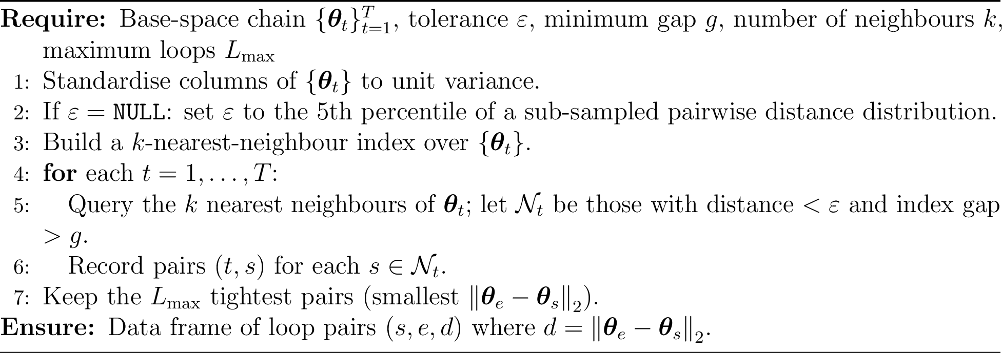
Loop detection is run per chain so that independent chains are never spliced. Pairs from all chains are pooled for the subsequent regression.
4.3 Transport map estimation↩︎
By Remark 5, the transport map for the GLMM class is diagonal with real entries: parallel transport scales each fiber coordinate independently. We therefore estimate \(J\) per-group scalars rather than a full \(J \times J\) matrix. Given \(M\) loop pairs with fiber start values \(\alpha_{s_k,j}\) and end values \(\alpha_{e_k,j}\), the weighted least squares estimate for group \(j\) is \[\hat{\rho}_j = \frac{\sum_{k=1}^{M} w_k\, \alpha_{e_k,j}\, \alpha_{s_k,j}}{\sum_{k=1}^{M} w_k\, \alpha_{s_k,j}^2 + \delta}, \label{eq:wls95H}\tag{7}\] where \(w_k\) are loop weights and
\(\delta > 0\) is a small ridge penalty. We write \(\hat{P} = \mathrm{diag}(\hat{\rho}_1, \ldots, \hat{\rho}_J)\). The fibr implementation retains the unrestricted \(J \times J\) estimator \(\hat{P} = (E W S^\top)(S W S^\top + \delta I)^{-1}\) as an option (structure = "full") for models with genuinely coupled fibers, but for diagonal-transport
models the full estimator fits \(J^2\) parameters to \(M\) noisy pairs and manufactures spurious off-diagonal structure, including spurious complex eigenvalues that can be mistaken for
rotational holonomy. All results in this paper use the diagonal estimator.
Weights are based on loop tightness: \(w_k \propto \exp(-d_k / \bar{d})\), where \(d_k = \left\|\boldsymbol{\theta}_{e_k} - \boldsymbol{\theta}_{s_k}\right\|_2\) and \(\bar{d}\) is the mean distance, so that tighter loops (better approximations to true closed loops) contribute more.
4.3.0.1 Residualisation.
Before estimating \(\hat{P}\), the fiber draws are residualised against the base draws via OLS, removing the linear base-to-fiber effect (e.g., \(\alpha_j \approx \mu\) in the centred GLMM). This isolates the vertical fiber component where geometric holonomy lives.
4.3.0.2 Interpretation.
The model \(\boldsymbol{\alpha}_e \approx P \boldsymbol{\alpha}_s\) is the simplest linear summary of loop-conditional dependence. For a well-mixed chain the endpoints are independent draws from the same conditional, so \(\hat{\rho}_j \approx 0\); a slowly mixing chain gives \(\hat{\rho}_j\) closer to unity. Note that geometric holonomy would also have produced \(\hat{\rho}_j \neq 0\), but with a loop-orientation- and area-dependent signature; since the connection is flat, no such geometric contribution exists, and any nonzero \(\hat{\rho}_j\) is conditional autocorrelation. This is what the attribution test of Section 4.7 confirms.
4.4 Per-group dependence coefficients and scalar summary↩︎
The estimated coefficients \(\hat{\rho}_1, \ldots, \hat{\rho}_J\) are read as follows:
\(\hat{\rho}_j \approx 0\): loop endpoints are approximately independent draws from the conditional posterior; the chain mixes faster than the loop time-scale and no signal survives.
\(\hat{\rho}_j\) substantially above 0: the fiber retains loop-conditional dependence at the loop time-scale. Under flatness this is conditional autocorrelation; the attribution step (Section 4.7) and the gap profile (Section 4.6) confirm there is no additional geometric component.
\(\hat{\rho}_j > 1\): indicates numerical instability or insufficient residualisation rather than a genuine effect.
The mean coefficient \(\bar{\rho} = J^{-1}\sum_j \hat{\rho}_j\) is our primary scalar summary, ranging from 0 (independent endpoints) toward 1 (full persistence). The Frobenius deviation \(\left\|\hat{P} - I\right\|_F\) is also reported but is a less discriminating summary: it equals \(\sqrt{J}\) in both the \(P \approx 0\) and \(P \approx I\) limits. Because the coefficients are group-aligned, \(\hat{\rho}_j\) can be compared directly with per-group analytic quantities: the prior fraction \(\pi_j\) 13 and the integrated transport prediction (Section 4.7).
4.5 Bootstrap uncertainty↩︎
Uncertainty is quantified by resampling loop pairs with replacement. For each of \(B\) bootstrap replicates, equation 7 is re-solved on the resampled pairs, and the resulting factors are recorded. Because the diagonal estimator preserves group identity, the bootstrap distribution of each \(\hat{\rho}_j\) is directly interpretable as per-group uncertainty, displayed as intervals on the per-group transport plot.
4.6 Gap sensitivity↩︎
The minimum gap \(g\) sets the time-scale at which loops are detected. If \(g\) is inside the integrated autocorrelation time (IACT) of the fiber chain, \(\hat{\rho}_j\) is dominated by ordinary autocorrelation; as \(g\) grows past the IACT, the autocorrelation contribution decays. Had the connection been curved, a systematic transport contribution would re-accumulate on every loop regardless of elapsed time and persist beyond the IACT; the gap profile was designed to expose such a component. Flatness implies there is none, and the profiles bear this out. We report \(\hat{\rho}_j\) as a profile over a grid of gaps (e.g.\(g \in \{3, 10, 25, 50\}\)) rather than at a single value, alongside the estimated IACT of the base and fiber chains. Two components can contribute to a signal surviving at \(g\) beyond the IACT: ordinary autocorrelation (decays with gap) and residualisation leakage (gap-independent, arising because OLS removes only the linear base-to-fiber dependence, while loop endpoints share the same base point and hence the same nonlinear conditional mean). A negative-control experiment reported in Section 4.7 separates these contributors empirically.
4.7 Attribution: empirical transport vs.integrated connection↩︎
A sharper test of the geometric interpretation bypasses the transport factors entirely. For each detected loop, integrate_transport() numerically integrates the analytic connection 4 along the actual chain
trajectory between the loop endpoints, producing a per-loop, per-group prediction of the fiber displacement attributable to parallel transport, together with the signed enclosed area of the base trajectory. Holonomy predicts displacements whose
sign tracks loop orientation and whose magnitude tracks the enclosed area and local curvature \(F_j\); generic autocorrelation predicts displacements uncorrelated with orientation and area.
On the sparse GLMM benchmark analysed here, this attribution test yields a null result. Regressing empirical displacement on the integrated-connection prediction gives slopes near zero for all groups (range \(-0.001\) to \(0.005\); one borderline significant at \(p = 0.025\)), and empirical displacements show no dependence on signed loop area in any group.
Two caveats scope this null. Test harshness: integrated parallel-transport predictions reach \(|\Delta\alpha| \approx 100\)–\(200\) against observed displacements of \(2\)–\(5\), because the linear-transport approximation breaks down along long, jagged MCMC paths through high-curvature regions. A restricted test on only the shortest, tightest loops (length \(\leq 50\), tightest distance quartile) also yields null results: 38 loops survived the filter and per-group slopes are of order \(10^{-5}\) per posterior SD.
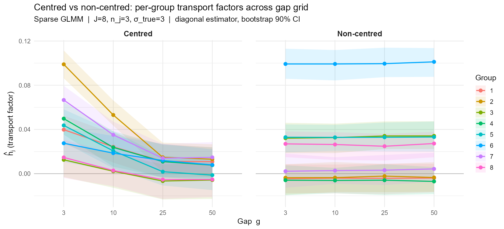
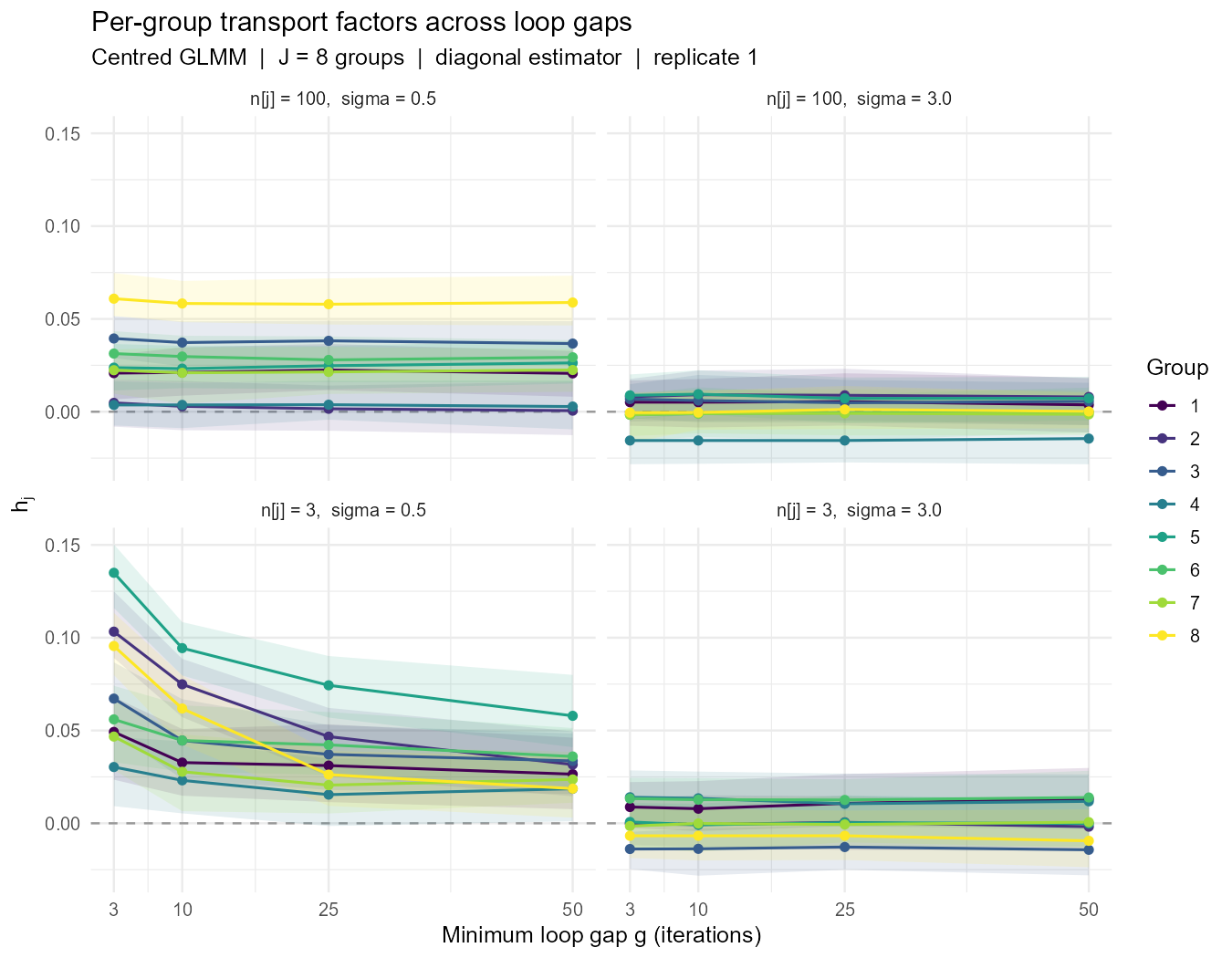
Negative control: for each gap \(g\), we construct matched-gap control pairs chosen to have large base distance (above the median of pairwise distances at that gap). On the prior-dominated cell (\(n_j = 3\), \(\sigma_\text{true} = 0.5\), high \(\pi_j\)), true loops give \(\bar{\rho}_j \approx 0.03\)–\(0.07\) while controls give \(\bar{\rho}_j \approx 0\): base-closure conditioning carries signal in exactly the cell where \(\pi_j\) predicts it. On the likelihood-dominated cell (\(\sigma_\text{true} = 3.0\), low \(\pi_j\)), both arms give \(\bar{\rho}_j \approx 0\). Figure 3 shows the full gap profile for all four experimental cells: the contrast between true-loop \(\hat{\rho}_j\) and the near-zero control band is confined to the high-\(\pi_j\) cell, in quantitative agreement with the analytic prediction.
This null is exactly what the flatness of the connection (Proposition 4) requires: there is no curvature, so there is no parallel-transport displacement for the chain to track, whether or not the sampler follows horizontal lifts. The geometry’s chain-level signature is instead excess conditional autocorrelation localised in prior-dominated groups—precisely what base-closure conditioning isolates and what the analytic \(\pi_j\) predicts. The analytic \(\pi_j\) is the primary and more robust diagnostic output: it requires no chain-based estimation, is free of residualisation leakage, and directly identifies which groups will show elevated \(\hat{\rho}_j\). The chain-based \(\hat{\rho}_j\) and its gap-sensitivity profile serve as empirical corroboration of the \(\pi_j\) prediction, confirming that the conditional dependence is detectable in actual chains, but \(\pi_j\) remains the headline flag. The diagnostic workflow (loop detection, estimation of \(\hat{\rho}_j\), and gap-sensitivity profiling) remains a valid probe of loop-conditional fiber dependence; flatness tells us that what it measures is conditional autocorrelation rather than holonomy.

4.8 Comparison: centred vs.non-centred↩︎
Figure 4 shows the per-group dependence coefficients across the gap grid for the centred and non-centred parameterisations of a sparse logistic GLMM (\(J = 8\) groups, \(n_j = 3\) observations each, \(\sigma_\text{true} = 3\)). At the shortest gap (\(g = 3\)), the centred chain shows a modestly larger mean coefficient (\(\bar{\rho} \approx 0.044\)) than the non-centred chain (\(\bar{\rho} \approx 0.022\)). The centred profile decays with gap (to \(\approx 0.005\) at \(g = 50\)), while the non-centred profile is flat across all gaps (\(\approx 0.022\)–\(0.023\)). The gap-independence of the non-centred factors, for a parameterisation in which \(\tilde{\alpha}_j\) is conditionally independent of \((\mu,\sigma)\) by construction, is consistent with residualisation leakage rather than geometric signal (Section 4.7). At long gaps the centred profile falls below the non-centred level; the short-gap excess in the centred chain (\(\approx 0.044\) at \(g=3\) vs \(\approx 0.005\) at \(g=50\)) is the autocorrelation contribution that decays with lag, while the flat non-centred baseline (\(\approx 0.022\)–\(0.023\) across all gaps) is the leakage floor, confirmed by the negative-control experiment.
5 Analytic Connection for the Centred Logistic GLMM↩︎
5.1 Model↩︎
We work throughout with the two-level logistic GLMM: \[\begin{align} y_{ji} &\sim \mathrm{Bernoulli}\!\left(\text{logit}^{-1}(\alpha_j + \boldsymbol{x}_{ji}^\top\boldsymbol{\beta})\right), \quad j \in [J],\; i = 1,\ldots,n_j, \tag{8} \\ \alpha_j &\sim \mathcal{N}(\mu, \sigma^2), \tag{9} \\ \mu &\sim \mathcal{N}(0, 25), \quad \sigma \sim \text{Exponential}(1), \quad \boldsymbol{\beta} \sim \mathcal{N}(\boldsymbol{0}, 4I). \tag{10} \end{align}\] The base space is \(\mathcal{B}= \mathbb{R}\times \mathbb{R}_{>0}\) with coordinates \((\mu, \sigma)\), and the fiber is \(\mathbb{R}^J\) with coordinates \(\boldsymbol{\alpha} = (\alpha_1,\ldots,\alpha_J)\). We write \(p_{ji} = \text{logit}^{-1}(\alpha_j + \boldsymbol{x}_{ji}^\top\boldsymbol{\beta})\) for the success probability of observation \(i\) in group \(j\).
5.2 Fisher metric blocks↩︎
We instantiate the block metric 2 for the GLMM. Because the logistic link is canonical, the observed information used below equals the expected Fisher information (Section 3), so naming these “Fisher metric blocks” is unambiguous here.
Proposition 2 (Fisher metric blocks for the centred GLMM). The negative Hessian of the log-posterior for model 8 –10 has the following blocks, evaluated at a single parameter point \((\mu, \sigma, \boldsymbol{\alpha}, \boldsymbol{\beta})\): \[\begin{align} G_{FF,jj} &= \frac{1}{\sigma^2} + \sum_{i=1}^{n_j} p_{ji}(1-p_{ji}), \label{eq:GFF} \\ G_{BF,j1} &= -\frac{1}{\sigma^2}, \quad\text{(base direction: \mu)} \label{eq:GBF95mu} \\ G_{BF,j2} &= -\frac{2(\alpha_j - \mu)}{\sigma^3}, \quad\text{(base direction: \sigma)} \label{eq:GBF95sigma} \end{align}\] {#eq: sublabel=eq:eq:GFF,eq:eq:GBF95mu,eq:eq:GBF95sigma} where \(G_{FF}\) is diagonal and \(G_{BF} \in \mathbb{R}^{J \times 2}\).
Proof. The log-posterior is \[\log p \propto \sum_{j \in [J]}\sum_{i=1}^{n_j} \bigl[y_{ji}\log p_{ji} + (1-y_{ji})\log(1-p_{ji})\bigr] - \sum_j \frac{(\alpha_j - \mu)^2}{2\sigma^2} - J\log\sigma - \text{priors on } \mu, \sigma, \boldsymbol{\beta}.\] Taking second derivatives: the cross term between \(\alpha_j\) and \(\alpha_k\) (\(j \neq k\)) vanishes because observations within group \(j\) do not depend on \(\alpha_k\). The diagonal \(\partial^2/\partial\alpha_j^2\) gives ?? . Cross terms \(\partial^2/\partial\alpha_j\,\partial\mu\) and \(\partial^2/\partial\alpha_j\,\partial\sigma\) give ?? and ?? respectively, from the prior term \(-(\alpha_j - \mu)^2/(2\sigma^2)\). ◻
Remark 3. The full base–base block \(G_{BB}\) is not positive definite outside the posterior mode in the centred parameterisation. This is the fingerprint of the funnel: the realised geometry of the total space is indefinite in the \((\mu, \sigma)\) directions when the chain is in the neck of the funnel. The indefiniteness is confined to \(G_{BB}\), however; the fiber block \(G_{FF,jj} = 1/\sigma^2 + \sum_i p_{ji}(1-p_{ji})\) is strictly positive throughout, so the connection \(A= -G_{FF}^{-1}G_{BF}\) and its \(G\)-orthogonality are globally well-defined and never see the funnel. This is the two-pathologies distinction already visible in the metric: the fiber geometry is always benign, the funnel is purely base-space. The SoftAbs regularisation [14] resolves the base indefiniteness for the RMHMC sampler (Section 2.2).
5.3 Connection form↩︎
From 3 and Proposition 2, the connection coefficients are: \[\begin{align} A_{j,\mu} &= \frac{1}{\sigma^2 G_{FF,j}}, \tag{11} \\ A_{j,\sigma} &= \frac{2(\alpha_j - \mu)}{\sigma^3 G_{FF,j}}. \tag{12} \end{align}\] Both depend on the current fiber point \(\alpha_j\), confirming that the connection is genuinely non-linear.
5.4 Curvature: linearised and full↩︎
Proposition 3 (Curvature of the linearised connection). Let \(\tilde{A}(\boldsymbol{\theta}) := A(\boldsymbol{\theta}, \boldsymbol{\alpha}_0)\) be the fiber-frozen linearisation of \(A\) at a fixed fiber point \(\boldsymbol{\alpha}_0\). Its curvature 5 , for the centred GLMM, is \[F_j = \frac{\partial A_{j,\sigma}}{\partial \mu} - \frac{\partial A_{j,\mu}}{\partial \sigma} = -\frac{2}{\sigma^5 G_{FF,j}^2}. \label{eq:curvature95glmm}\qquad{(1)}\] Equivalently, \(F_j\) is the exterior derivative of \(A\) taken with the fiber held fixed.
Proof. From 12 , noting that \(G_{FF,j}\) does not depend on \(\mu\) (the likelihood term involves \(\alpha_j\), \(\boldsymbol{\beta}\), and the data, but not \(\mu\)): \[\frac{\partial A_{j,\sigma}}{\partial \mu} = \frac{-2}{\sigma^3 G_{FF,j}}.\] From 11 , noting that \(\partial G_{FF,j}/\partial\sigma = -2/\sigma^3\) (from the prior term \(1/\sigma^2\)): \[\frac{\partial A_{j,\mu}}{\partial \sigma} = \frac{-2}{\sigma^3 G_{FF,j}} + \frac{1}{\sigma^2} \cdot \frac{2/\sigma^3}{G_{FF,j}^2} = \frac{-2}{\sigma^3 G_{FF,j}} + \frac{2}{\sigma^5 G_{FF,j}^2}.\] Subtracting: \(F_j = -2/(\sigma^5 G_{FF,j}^2)\). ◻
This linearised curvature is always negative (\(F_j < 0\)), and \(|F_j|\) grows as the prior dominates (small \(\sigma\), few data). Read naively, this suggests a contractive holonomy of \(\tilde{A}\) that worsens as the prior tightens. But \(\tilde{A}\) is not the connection the sampler would have to follow; the true connection is the fiber-dependent \(A\). By Proposition 1 its full curvature vanishes; for the GLMM this can be seen explicitly, and the cancellation is instructive.
Proposition 4 (Flatness of the GLMM connection, instance of Proposition 1). The full curvature of the metric-orthogonal Ehresmann connection \(A\) of 11 –12 , including the vertical (fiber-derivative) terms, is identically zero for every group \(j\): \[F_j^{\mathrm{full}} = \underbrace{\frac{\partial A_{j,\sigma}}{\partial \mu} - \frac{\partial A_{j,\mu}}{\partial \sigma}}_{=\,-2/(\sigma^5 G_{FF,j}^2)} + \underbrace{A_{j,\mu}\frac{\partial A_{j,\sigma}}{\partial \alpha_j} - A_{j,\sigma}\frac{\partial A_{j,\mu}}{\partial \alpha_j}}_{=\,+2/(\sigma^5 G_{FF,j}^2)} = 0 . \label{eq:flat}\qquad{(2)}\] Consequently the horizontal distribution is integrable (Frobenius), and since the base \(\mathcal{B}= \mathbb{R}\times \mathbb{R}_{>0}\) is simply connected, the holonomy of every loop is trivial: a global flat trivialisation exists.
Proof. The first pair is Proposition 3. For the vertical pair, write \(S_j = \sum_i p_{ji}(1-p_{ji})\) so that \(G_{FF,j} = 1/\sigma^2 + S_j\) and \(\partial G_{FF,j}/\partial\alpha_j = S_j' = \sum_i p_{ji}(1-p_{ji})(1-2p_{ji})\). Then \[A_{j,\mu}\frac{\partial A_{j,\sigma}}{\partial \alpha_j} = \frac{1}{\sigma^2 G_{FF,j}}\!\left[\frac{2}{\sigma^3 G_{FF,j}} - \frac{2(\alpha_j-\mu)S_j'}{\sigma^3 G_{FF,j}^2}\right] = \frac{2}{\sigma^5 G_{FF,j}^2} - \frac{2(\alpha_j-\mu)S_j'}{\sigma^5 G_{FF,j}^3},\] \[A_{j,\sigma}\frac{\partial A_{j,\mu}}{\partial \alpha_j} = \frac{2(\alpha_j-\mu)}{\sigma^3 G_{FF,j}} \!\left[-\frac{S_j'}{\sigma^2 G_{FF,j}^2}\right] = -\frac{2(\alpha_j-\mu)S_j'}{\sigma^5 G_{FF,j}^3}.\] The \(S_j'\) terms cancel in the difference, leaving \(+2/(\sigma^5 G_{FF,j}^2)\), which is exactly the negative of the first pair. Hence \(F_j^{\mathrm{full}} = 0\). ◻
Remark 4 (Why the linearised curvature is nonzero). The discrepancy between \(F_j \neq 0\) and \(F_j^{\mathrm{full}} = 0\) is the vertical variation of \(A\) along the transported fiber. Freezing the fiber (equivalently, holding \(G_{FF,j}\) at its value at the loop centre) discards the second pair in ?? and recovers the nonzero \(F_j\). This is precisely what the synthetic-loop validation of Section 5.6 does, so the “holonomy” it reports is the holonomy of the linearised connection, not of the true one. We
confirm the result numerically in data-raw/verify_flat_connection.R: integrating the true transport ODE around closed loops returns displacement of order \(10^{-14}\), while freezing \(G_{FF,j}\) reproduces the linearised holonomy of Figure 5. Both \(F_j\) and \(F_j^{\mathrm{full}}\) are curvatures of the Ehresmann
connection (iii) of Section 3.4; neither is the Riemann curvature of the Fisher–Rao metric, which is hyperbolic and nonzero and which the flatness of \(A\) does not
affect.
Remark 5 (The structure group is abelian: no rotational holonomy). Because \(G_{FF}\) is diagonal and the rows of \(G_{BF}\) decouple across groups, parallel transport acts on each fiber coordinate independently: any loop’s transport is a per-group scaling \(\alpha_j \mapsto h_j \alpha_j\) with \(h_j \in \mathbb{R}_{>0}\) (and, by Proposition 4, \(h_j = 1\) for the true connection). The structure group of this bundle is abelian, and genuinely rotational* holonomy (complex transport eigenvalues) is impossible for this model class. This has a practical consequence for estimation: the diagnostic’s dependence matrix \(\hat{P}\) is diagonal with real entries, so it should estimate \(J\) scalars rather than a full \(J \times J\) matrix (Section 4.3).*
5.5 Prior fraction↩︎
The ratio of the prior precision to the total fiber precision \[\pi_j = \frac{1/\sigma^2}{G_{FF,j}} = \frac{1/\sigma^2}{1/\sigma^2 + \sum_{i=1}^{n_j}p_{ji}(1-p_{ji})} \label{eq:prior95fraction}\tag{13}\] takes values in \((0,1)\) and measures how much of the fiber metric at group \(j\) is attributable to the prior. When \(\pi_j \to 1\) the prior dominates (sparse data or large \(\sigma\)); when \(\pi_j \to 0\) the likelihood dominates. This is exactly the pooling factor \(\omega\) of [8], the fraction of a group’s posterior precision contributed by the prior: their \(\omega = 1 - \sigma_\alpha^2/(\sigma_\alpha^2 + \sigma_y^2)\) is \((1/\sigma_\alpha^2)/(1/\sigma_\alpha^2 + n_j/\sigma_y^2)\), which is Equation 13 for the Gaussian case. It is thus a classical quantity, not a new one: recoverable by hand from a fitted multilevel model’s variance components and per-group information, and reported in related (population-level) form as the intraclass correlation by standard tools. What we add is its geometric derivation as the residual obstruction once the connection is flat, and its per-coordinate computation; the package simply returns it. (We use “pooling factor” rather than “shrinkage factor” deliberately: some authors call the complement \(1-\pi_j\) the shrinkage factor, a usage [8] flag as confusing, since a shrinkage factor of zero then means complete pooling.) It is also the per-group form of the prior/likelihood balance that [1] tied to the optimal parameterisation. In plain terms, \(\pi_j\) is the share of what the posterior knows about group \(j\) that comes from the prior rather than from that group’s own data: near 1, the data barely constrain the group and a non-centred parameterisation helps; near 0, the group is well identified and centring is fine. What the bundle derivation adds locally is the observation that \(\pi_j\) is determined by prior precision \(1/\sigma^2\) rather than prior variance — the source of the non-monotone behaviour in \(\sigma\) documented in Section 6. Substituting into the linearised curvature ?? gives \(|F_j| = 2\pi_j^2/\sigma\): even the spurious linearised curvature is controlled by \(\pi_j\), so the diagnostic and the analytic flag agree on where any signal must concentrate.
Remark 6. The prior fraction \(\pi_j\) is computed analytically from a subsample of posterior draws and serves as a diagnostic in its own right: groups with \(\pi_j >
0.6\) are good candidates for non-centred reparameterisation (Section 7.4). This is the geometric basis for the per-group parameterisation advice implemented in fibr.
5.6 Synthetic loop validation↩︎
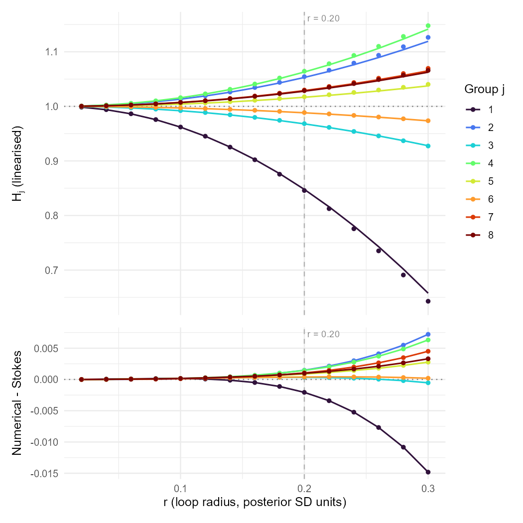
We check the linearised curvature formula ?? against Stokes’ theorem 6 using synthetic circular loops in \((\mu, \sigma)\) space, bypassing any MCMC noise. We stress that this validates the linearised connection only: the integration below holds the fiber fixed at \(\boldsymbol{\alpha}_0\) (equivalently, freezes \(G_{FF}\)), which is the linearisation whose curvature is nonzero. Integrating the true connection, with \(G_{FF}\) updated as the fiber moves, returns zero displacement to integrator precision, consistent with Proposition 4.
For a circle of radius \(r\) centred at the posterior mean \((\mu_0, \sigma_0, \boldsymbol{\alpha}_0, \boldsymbol{\beta}_0)\):
Numerically integrate the ODE 4 around the circle (discretised into \(n_s = 400\) steps) to obtain \(\Delta\alpha_j^{\text{num}}\).
Compute the first-order Stokes prediction \(\Delta\alpha_j^{\text{Stokes}} = F_j(\mu_0,\sigma_0,\boldsymbol{\alpha}_0) \cdot \pi r^2\).
Figure 5 shows the comparison for radii \(r \in [0.02, 0.30]\) (approximately \(0.02\)–\(0.30\) posterior standard deviations), displayed separately for each of the \(J = 8\) groups. The numerically integrated linearised transport and its first-order Stokes prediction agree closely for \(r \leq 0.20\) across all groups, and diverge for larger radii where the quadratic Stokes term becomes relevant. The divergence is not uniform: groups with higher \(|F_j|\) depart from the linear Stokes prediction at smaller \(r\), while groups with near-flat linearised curvature remain in agreement throughout the range. This agreement validates the internal consistency of the connection 11 –12 and the linearised curvature ?? . It is not evidence of geometric holonomy: by Proposition 4 the true holonomy is zero, and Figure 5 reports the linearised object that the freezing of \(\boldsymbol{\alpha}_0\) creates.
6 Simulation Study↩︎
6.1 Design↩︎
We ran a \(4 \times 4\) factorial simulation study varying observations per group \(n_j \in \{3, 10, 30, 100\}\) and true hierarchical standard deviation \(\sigma_\text{true} \in \{0.5, 1.0, 2.0, 3.0\}\), with \(J = 8\) groups and 10 replicates per cell (160 Stan fits in total). For each replicate: data were simulated from model 8 –10 with \(\boldsymbol{\beta}_\text{true} = (0.8, -0.5)\), \(\mu_\text{true} = 0\); the centred Stan model was fitted with
4 chains \(\times\) 2,000 post-warmup iterations; the dependence diagnostic (diagonal estimator) was evaluated at each gap in the grid \(g \in \{3, 10, 25, 50\}\), alongside the estimated
IACT of the base and fiber chains; and the analytic prior fraction was computed from 200 subsampled draws via compute_connection().
The primary scalar is the mean dependence coefficient \(\bar{\rho} = J^{-1}\sum_j \hat{\rho}_j\) at each gap. As established in Section 4, this is near 0 when loop endpoints are independent (well-mixed at the loop time-scale) and grows toward 1 with loop-conditional persistence. The gap profile separates the two contributors that flatness leaves: ordinary autocorrelation, which decays once \(g\) exceeds the IACT, and residualisation leakage, which is gap-independent (Section 4.7). With flatness established analytically, the simulation is not a search for a geometric signal but a check of two things: that the conditional dependence \(\pi_j\) predicts is detectable and correctly localised in finite chains, and that it is geometrically separable from the funnel.
6.2 Results↩︎
The headline of the study is the geometric separation of the two pathologies (the non-monotone \(\sigma\) behaviour below); the theory–empirical agreement confirms that the predicted dependence is detectable in finite chains, but it is the weaker, expected half of the picture.
6.2.0.1 Heatmap.
Figure 6 shows the median \(\bar{\rho}\) over 10 replicates. The signal is strongest in the upper-left corner (\(n_j = 3\), \(\sigma_\text{true} = 0.5\)–\(1.0\)) and decreases monotonically with \(n_j\) at every \(\sigma_\text{true}\) value.
6.2.0.2 The \(\sigma\)-direction is non-monotone and illuminating.
Within the \(n_j = 3\) row, \(\bar{\rho}\) is highest at \(\sigma_\text{true} = 0.5\)–\(1.0\) (0.040 and 0.036 at the
headline gap \(g = 50\)) and drops sharply for \(\sigma_\text{true} \in \{2.0, 3.0\}\) (0.013, 0.015). This is not a failure of the diagnostic but a genuine distinction: the prior fraction
\(\pi_j = (1/\sigma^2)/G_{FF,j}\) is determined by the ratio of prior precision to total precision. Increasing \(\sigma\) reduces \(1/\sigma^2\),
which reduces the prior fraction (Table 1) even as it worsens the funnel. The funnel pathology (large \(\sigma\), slow mixing in \(\sigma\)) and the
coupling pathology (large \(\pi_j\), strong base-conditional fiber dependence) are related but distinct: the former is a problem of base-space geometry; the latter is a problem of the base–fiber coupling. Standard
diagnostics (divergences, low ESS) detect the former; the per-group \(\hat{\rho}_j\) and analytic \(\pi_j\) from fibr localise the coupling pathology to specific groups, its
chain-level signature being structured conditional autocorrelation, per Section 4.7.
![Figure 6: Simulation study: median mean dependence coefficient \bar{\rho} over 10 replicates, by gap g. Tile labels show median [Q25, Q75]. The signal (dark tiles) is concentrated in the prior-dominated upper-left corner (n_j small, \sigma_\text{true} small to moderate). The \sigma-axis is non-monotone: the coupling signal is driven by prior precision 1/\sigma^2, not by \sigma itself.](/article/2606.19655/figures/simstud_heatmap.png "fig:")
6.2.0.3 Theory vs.empirical.
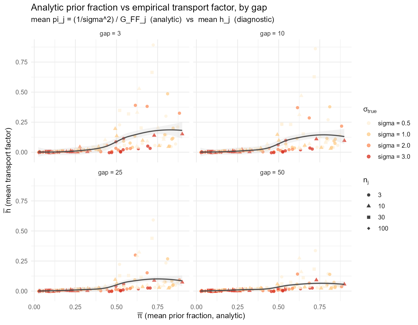
Figure 7 plots the mean prior fraction \(\bar{\pi}\) (analytic) against \(\bar{\rho}\) (diagnostic), faceted by gap, for all 640 cell-replicate–gap combinations. The LOESS trend is positive, consistent with the analytic prior fraction being a leading predictor of the empirical signal. Given flatness, we read this straightforwardly: prior dominance slows mixing, so \(\pi_j\) predicts the strength of the conditional autocorrelation that the diagnostic measures, with no geometric component to disentangle. The attribution test of Section 4.7 yielded the corresponding null result; this figure establishes that the analytic quantity and the empirical diagnostic move together across the design. Scatter around the trend reflects simulation variability in the data and chain.
| \(n_j\) | \(\sigma_\text{true}\) | \(\bar{\rho}\) | \(\rho_{\max}\) | \(\bar\pi\) | % Div |
|---|---|---|---|---|---|
| 3 | 0.5 | 0.040 | 0.090 | 0.784 | 100 |
| 3 | 1.0 | 0.036 | 0.070 | 0.802 | 100 |
| 3 | 2.0 | 0.013 | 0.028 | 0.537 | 100 |
| 3 | 3.0 | 0.015 | 0.033 | 0.533 | 100 |
| 10 | 0.5 | 0.034 | 0.057 | 0.635 | 100 |
| 10 | 1.0 | 0.023 | 0.044 | 0.444 | 100 |
| 10 | 2.0 | 0.011 | 0.026 | 0.276 | 90 |
| 10 | 3.0 | 0.005 | 0.016 | 0.250 | 40 |
| 30 | 0.5 | 0.032 | 0.062 | 0.474 | 100 |
| 30 | 1.0 | 0.010 | 0.022 | 0.166 | 50 |
| 30 | 2.0 | 0.002 | 0.016 | 0.113 | 0 |
| 30 | 3.0 | 0.002 | 0.015 | 0.094 | 0 |
| 100 | 0.5 | 0.011 | 0.034 | 0.172 | 50 |
| 100 | 1.0 | 0.001 | 0.010 | 0.051 | 10 |
| 100 | 2.0 | 0.001 | 0.013 | 0.029 | 0 |
| 100 | 3.0 | 0.001 | 0.013 | 0.037 | 0 |
7 What to Do About It: Guidance for Practitioners↩︎
The diagnostic identifies which groups suffer a geometric obstruction and why; this section addresses what a practitioner should do next. The good news is that the indicated remedies are well-established methods that require no new sampler: the geometric analysis tells us when and where to apply them.
7.1 Per-group (partial) non-centering, guided by the prior fraction↩︎
The prior fraction \(\pi_j\) 13 is precisely the quantity that determines the optimal parameterisation of group \(j\) [2], [11]. Groups with \(\pi_j\) near 1 (prior-dominated) should be non-centred; groups with \(\pi_j\) near 0 (data-dominated) should remain centred; intermediate groups benefit from partial non-centering, \[\alpha_j = \mu + \sigma^{w_j}\,\tilde{\alpha}_j^{(w_j)}, \qquad w_j \in [0, 1],\] which interpolates between the centred (\(w_j = 0\)) and non-centred (\(w_j = 1\)) coordinates. For the Gaussian case the optimal partial non-centring weight is classical and closed-form [11]; for non-Gaussian models [7] instead learn \(w_j\) by stochastic variational optimisation (the VIP algorithm). The geometric analysis of Section 5 supplies the GLMM analogue in closed form: \(w_j \approx \pi_j\) evaluated at the posterior mean, recovering the variational weight from a pilot run rather than an optimisation. This is the primary practical payoff of the framework: a cheap, analytic, per-group parameterisation rule with a clear justification. We tested this rule directly on a mixed design. Table 2 reports median min-ESS (over all parameters, \(J = 8\) groups, 10 replicates) for the centred, half (\(w_j = 0.5\)), non-centred, and \(w_j = \pi_j\) parameterisations, across uniform-sparse, mixed, and uniform-dense designs at \(\sigma \in \{1, 2\}\). Two findings emerge, both consistent with the two-pathologies view (Section 9).
(i) On min-ESS the non-centred parameterisation wins in every cell. The minimum is taken over all parameters and is dominated by \(\sigma\), whose centred geometry retains a funnel that non-centering removes regardless of group size; in the range tested (\(\sigma \in \{1,2\}\), \(n_j \in \{3,50\}\)) non-centering is never harmful enough elsewhere to forfeit this advantage. The \(\pi_j\)-adaptive rule interpolates in the right direction: at \(\sigma = 1\) sparse, \(\pi_j \approx 0.8\), so its weights are near-non-centred and it reaches min-ESS \(2381\), far above centred (\(187\)) and half (\(1071\)), but it does not match full non-centring (\(3327\)), because the residual centering left by \(w_j < 1\) leaves some \(\sigma\)-funnel. We therefore do not claim \(w_j = \pi_j\) beats both uniform choices: in this regime it is a safe interpolator that improves on the worse uniform choice and moves toward the better as \(\pi_j\) rises, not a uniform winner.
(ii) The prior fraction nonetheless does its job at the level it speaks to, the per-group fiber. On per-group \(\alpha_j\) ESS (Figure 9), \(w_j = \pi_j\) sits at or near the best method for every group: it non-centres exactly the prior-dominated groups whose centred \(\alpha_j\) ESS would otherwise lag, and leaves data-dominated groups alone. The min-ESS bottleneck is the \(\sigma\)-funnel, a base-space pathology that no per-group fiber reparameterisation can touch; the gap between per-group success and min-ESS is the two-pathologies distinction made concrete. A practical aside visible in the same data: in the mixed design the data-rich groups stabilise \(\sigma\) and lift \(\alpha_j\) ESS for all methods, so a few well-identified groups can make centring tolerable for the sparse ones. The value of \(w_j = \pi_j\) over a single uniform choice is thus robustness across regimes (a uniform choice is optimal only within its own regime, and very large \(n_j\) or \(\sigma \to 0\) would reverse non-centring’s advantage, cases not covered here) together with its role as an analytic per-group diagnostic from a single pilot run. This is the typical situation in unbalanced multilevel and panel data, where groups carry very different numbers of observations; there a per-group choice can matter, whereas balanced designs are usually well served by a single uniform parameterisation.
| Method | \(\sigma = 1.0\) | \(\sigma = 2.0\) | ||||
|---|---|---|---|---|---|---|
| 2-4(lr)5-7 | Sparse | Mixed | Dense | Sparse | Mixed | Dense |
| Centred (\(w_j = 0\)) | 187 | 1988 | 1559 | 609 | 1993 | 1395 |
| Half (\(w_j = 0.5\)) | 1071 | 2143 | 1768 | 1457 | 2173 | 1510 |
| Non-centred (\(w_j = 1\)) | 3327 | 2626 | 1858 | 2349 | 2467 | 1628 |
| \(w_j = \pi_j\) (adaptive) | 2381 | 2119 | 1621 | 1432 | 2082 | 1389 |

7.2 Interweaving (ASIS)↩︎
When no single parameterisation works for all groups, or when the practitioner prefers not to commit, the ancillarity–sufficiency interweaving strategy of [12] alternates centred and non-centred updates within each iteration. ASIS is provably robust exactly in the regime the diagnostic flags: where no single parameterisation suits every group simultaneously, because the prior fractions \(\pi_j\) are spread across the unit interval. By combining the sufficient (centred) and ancillary (non-centred) augmentations it is efficient whenever at least one is, group by group. For Stan users, the per-group rule of Section 7.1 is usually simpler to implement; ASIS is the method of choice for Gibbs-style samplers where both conditionals are tractable.
7.3 Marginalising the fiber↩︎
The coupling pathology lives in the base–fiber dependence; it can be removed entirely by integrating the fiber out. For the logistic GLMM the conditional posterior of each \(\alpha_j\) given \((\mu, \sigma, \boldsymbol{\beta})\) is log-concave, so a Laplace or adaptive quadrature approximation to the marginal likelihood of \((\mu, \sigma, \boldsymbol{\beta})\) is accurate and cheap [20]. Sampling the low-dimensional marginal and drawing \(\boldsymbol{\alpha} \mid \mu, \sigma, \boldsymbol{\beta}, y\) afterwards eliminates the connection rather than correcting for it, at the cost of an approximation whose error must be checked. Where it applies, this is the most direct remedy; the diagnostic identifies when the extra machinery is warranted.
7.4 The connection as a fixed linear reparameterisation↩︎
The connection can also be turned into a reparameterisation directly. Evaluating the coefficients \(\{A_{j,\mu}, A_{j,\sigma}\}\) at the posterior mean \((\mu_0, \sigma_0)\) and
introducing horizontally-corrected fiber coordinates \[\tilde{\alpha}_j = \alpha_j - A_{j,\mu}\,(\mu - \mu_0) - A_{j,\sigma}\,(\sigma - \sigma_0)
\label{eq:horiz95reparameterisation}\tag{14}\] removes the linear contribution of the base to the fiber, weakening the base-conditional dependence that \(\pi_j\) measures. This is not the
exact flat coordinate: by Proposition 1 that is the conditional score \(\partial_{\boldsymbol{\alpha}}\ell\), the
precision-weighted residual \((\alpha_j-\mu)/\sigma^2\) for the GLMM, which is nonlinear in the base. Equation 14 is its linearisation, with \(A\) frozen at the posterior mean and kept to first order in \((\mu-\mu_0,\sigma-\sigma_0)\). It is implemented in Stan as glmm_hconnected.stan and needs only the connection
coefficients as data. Table 3 compares effective sample size for the centred, non-centred, and horizontally-corrected models on the sparse GLMM benchmark (\(J=8\), \(n_j=3\), \(\sigma_\text{true}=3\)).
| Parameter | Centred | H-corrected | Non-centred |
|---|---|---|---|
| \(\mu\) | 39.6% | 90.6% | 41.7% |
| \(\sigma\) | 7.7% | 12.3% | 29.3% |
| \(\alpha[1]\) | 66.5% | 100.8% | 100.2% |
| \(\beta[1]\) | 60.8% | 70.6% | 86.4% |
The H-corrected parameterisation dominates on \(\mu\) (90.6% vs.% centred and 41.7% non-centred) and matches non-centred on \(\alpha[1]\): the linear correction removes the \(\mu\)–fiber coupling well, even though it is only the linearisation of the exact trivialisation. It is weaker on \(\sigma\) (12.3%) than non-centering (29.3%), but for a reason distinct from
linearisation error: \(\sigma\) is the funnel, a base-space pathology, and no fiber reparameterisation (the exact score map included) can touch it. Since \(\sigma\) is the
bottleneck here, plain non-centering wins on minimum ESS; the H-correction’s gains are on \(\mu\) and the fiber. We therefore present it as a diagnostic-driven illustration that the connection is directly actionable, not as
a replacement for non-centering, the per-group rule of Section 7.1 is the tool we recommend. The per-group rule is already used in the smoothbp change-point package [21], where \(\pi_j\) guides the parameterisation of each subject’s change-points; a worked example is in the package’s
reproduction materials, with a fuller treatment in a companion paper.
7.5 Connection-corrected proposals (proof of concept)↩︎
Finally, the connection \(A = -G_{FF}^{-1}G_{BF}\) is itself directly actionable: it prescribes how the fiber should co-move when the base moves to remain on the horizontal slice. The fibr package provides
horizontal_mcmc(), a block Metropolis-within-Gibbs sampler in which each base-block proposal \((\mu, \sigma) \to (\mu', \sigma')\) pre-displaces the fiber by \(\Delta\boldsymbol{\alpha} = A(\mu, \sigma, \boldsymbol{\alpha})\,
(\Delta\mu,\,\Delta\sigma)^\top\) before the joint accept/reject step. We include this as a proof of concept that the analytic connection is actionable at negligible cost, not as a recommended production sampler; for applied work the methods of
Sections 7.1–7.3 are mature, available in standard tooling, and should be preferred. Two cautions are warranted. First, naively applying the connection as a
deterministic pre-displacement without the corresponding Jacobian correction is biased: a simulation-based calibration check of that variant fails decisively, whereas the exactly-invertible Laplace transport and a reparameterised HMC in the
Laplace-standardised fiber both pass calibration. This is consistent with flatness: the correct “connection-aware” move is a reparameterisation, not a transport. Second, on the sparse benchmark the calibrated variants are correct but do not outperform
non-centred NUTS in effective sample size per gradient evaluation; they are a demonstration, not a faster sampler. A full treatment of connection-aware sampling (horizontal leapfrog HMC with \(A\) recomputed at every
leapfrog step, ergodicity analysis, and multi-model benchmarking) is developed in a companion paper.
7.6 Reading the prior fraction: influence and sensitivity↩︎
Beyond the centring decision, \(\pi_j\) is an inferential quantity: it is the share of group \(j\)’s posterior precision supplied by the prior, so it localises where prior choices can move conclusions. High-\(\pi_j\) groups are prior-dominated and are the ones to interrogate; low-\(\pi_j\) groups are prior-robust by construction. Two questions follow. Is \(\sigma\) well identified, or is \(\pi_j\) inheriting the hyperprior? Since \(\pi_j = 1/(1 + I_j\sigma^2)\), with \(I_j = G_{FF,j} - 1/\sigma^2\) the group’s own likelihood information, and \(\sigma\) is identified by the number of groups rather than the data per group, a refit under an alternative \(\sigma\)-prior shows whether the high-\(\pi_j\) groups move (a hyperprior artefact) or hold (a data statement). And for those groups, is the population-level prior they are shrunk toward one you would defend for a group with little data of its own? A fuller treatment for applied users is left to a separate paper.
Remark 7 (A frequentist reading). The shrinkage is not itself Bayesian: the REML/BLUP predictor of \(\alpha_j\) shrinks by the same factor, and the flat-prior limit \(\sigma \to \infty\) sends \(\pi_j \to 0\), recovering the per-group maximum-likelihood (no-pooling) estimate. That limit is also where the sparse group becomes awkward — with small \(I_j\) the no-pooling estimate has variance \(\sim 1/I_j\) and is barely admissible, and such groups are routinely discarded. A proper hierarchical prior retains them with a coherent posterior, and \(\pi_j\) states how much of the estimate rests on that prior rather than on the likelihood, making the evidence explicit instead of excluding the case.
8 The fibr R Package↩︎
The fibr package [13] centres on the prior fraction, the quantity this paper concludes is the operative one; it is the
maintained, user-facing tool and is distributed on CRAN. The geometric and sampler methods used to produce the figures (the analytic connection, the loop-conditional dependence diagnostic, the transport integrator, and the connection-corrected sampler)
accompany the paper as reproduction code under paper/ in the source repository: with the connection flat for this model class, they are demonstration apparatus rather than routine diagnostics, and they load by sourcing
paper/setup.R. Table 4 lists the package’s exported functions.
| Function | Description |
|---|---|
| prior_fraction() | Read-only per-coordinate prior fraction \(\pi_j\) (shrinkage / pooling factor) for a fitted hierarchical model, with an adapter for brms fits and a manual path for other Stan models. Reports which group-level coordinates are prior-dominated, without reparameterising or refitting. |
| smoothbp_advisor() | Fisher information decomposition for changepoint random effects in smoothbp fits; returns per-group prior fractions and parameterisation recommendations. |
The package itself depends only on posterior [22] for chain handling and ggplot2 for visualisation; the reproduction
code under paper/ additionally uses FNN for \(k\)-nearest-neighbour search, Matrix, deSolve, and a Stan backend (cmdstanr, [23]). While the connection and dependence machinery target the two-level logistic GLMM, the prior fraction is model-agnostic: prior_fraction() computes it per
coordinate for any fitted hierarchical model, with an adapter for brms fits, as a read-only report of which group-level estimates are prior-dominated (mostly shrinkage) rather than data-driven. Because the per-coordinate computation needs only
the fitted variance components and the per-observation working weights, it extends without special-casing to nested, crossed, and multi-level designs and to non-Gaussian families. This is the regime in which the intraclass correlation requires
case-specific conventions (a latent-scale residual for generalised models, a covariate value for random slopes, separate adjusted and unadjusted forms at each level), and the package’s tests verify the per-coordinate values against an independent
recomputation for nested, crossed, and three-level Gaussian and Bernoulli fits. Because it neither reparameterises nor refits, it carries none of the calibration burden of a reparameterisation and serves as a lightweight prior-influence diagnostic
alongside \(\hat{R}\) and effective sample size. The package is available at https://github.com/ABindoff/fibr.
9 Discussion↩︎
9.1 Coupling vs.the funnel: two distinct pathologies↩︎
The simulation study (Section 6) reveals two related but distinct pathologies, neither of which is geometric holonomy of \(A\). The funnel is a base-space pathology, and it is genuinely geometric: it reflects the intrinsic curvature of the base, whose Fisher–Rao metric is hyperbolic (connection (i) of Section 3.4). When \(\sigma\) is large, the posterior of \(\sigma\) is concentrated at small values (shrinkage) and the conditional distribution \(p(\boldsymbol{\alpha}|\mu,\sigma)\) is narrow, creating a highly non-isotropic target. HMC struggles because leapfrog steps that work in the wide region overshoot in the neck. The flatness of \(A\) says nothing about this curvature and does not remove it.
The second is a base–fiber coupling pathology: when \(\sigma\) is small (tight prior, high prior precision), the connection \(A_{j,\mu} = 1/(\sigma^2 G_{FF,j})\) is large, so the conditional posterior of \(\alpha_j\) tracks \(\mu\) tightly and the centred chain explores it slowly. It is tempting to read this as holonomy, a sampler that does not know the connection cannot make horizontally-corrected proposals, but Proposition 4 shows the connection is flat, so there is no holonomy to follow, and the key empirical finding (Section 4.7) confirms it: NUTS does not transport the fiber, and chain displacements \(\alpha_\text{end} - \alpha_\text{start}\) do not track any parallel-transport prediction. What remains is purely statistical: excess conditional autocorrelation. Prior-dominated groups (\(\pi_j\) large) retain loop-conditional fiber dependence that likelihood-dominated groups do not, and a negative-control experiment confirms this signal is tied to base-closure conditioning rather than to lag autocorrelation alone. The two pathologies can co-occur (sparse data and a wide prior create both a funnel and, at intermediate \(\sigma\), strong coupling), but they are separable: the funnel is a base-space curvature problem, while the coupling is captured entirely by the per-group prior fraction \(\pi_j\).
9.2 The connection is flat; curvature lives in the working metric↩︎
Proposition 1 settles a question an earlier draft of this paper left open. The metric-orthogonal connection is flat for any smooth hierarchical posterior, of any fiber dimension, with any prior — not because of conjugacy but because the fiber score is a first integral. In particular, correlated random effects, spatial or temporal fiber dependence, and vector-valued group effects with a non-diagonal prior covariance all give flat connections; they do not, contrary to what one might expect, produce rotational holonomy of the true connection. The only ways the metric-orthogonal connection fails to be flat are (i) where \(G_{FF}\) is singular (the fiber-degeneracy regime discussed below, where the foliation by score level sets breaks down and obstruction can genuinely re-enter) and (ii) when the connection is built from a metric other than the true Hessian. Case (ii) is not a defect but an opportunity: it is where genuine curvature lives.
Write \(A_M = -M_{FF}^{-1}G_{BF}\) for the distribution orthogonal with respect to a working metric \(M\): a fixed mass matrix, an empirical covariance, or the prior-only metric.
The score argument no longer applies, since \(M_{FF} \neq -\partial^2_{\boldsymbol{\alpha}}\ell\), and \(A_M\) is generically curved. We verify this in a two-fiber example: a bivariate group
effect \(\alpha\in\mathbb{R}^2\) with base-dependent prior correlation \(\Lambda(\boldsymbol{\theta}) = R(\theta_2)\mathrm{diag}(e^{\theta_1},e^{-\theta_1})R(\theta_2)^\top\) and a logistic
likelihood (so the posterior is non-Gaussian and \(G_{FF}\) is fiber-dependent). The metric blocks are computed in closed form and validated against automatic differentiation to machine precision (\(\sim 10^{-16}\)), and the holonomy operator \(H_M\) is obtained by integrating parallel transport with an adaptive high-order solver (DOP853, tolerance \(10^{-12}\)); the true Fisher connection returns to the identity at the integrator floor (\(\left\|H_M-I\right\|_F \sim 10^{-13}\)) at every loop size, confirming Proposition 1 numerically. Taking \(M_{FF}\) to be the identity instead yields a holonomy operator with complex eigenvalues \(0.986 \pm 0.167\,i\); an anisotropic fixed metric \(\mathrm{diag}(1,3)\) gives \(0.998 \pm 0.071\,i\). Crucially, \(\left\|H_M -
I\right\|_F\) grows as the first power of the enclosed base area (fitted log-log slopes \(1.08\) and \(0.99\), Figure 10), the hallmark
of genuine curvature (leading-order holonomy \(=\) curvature \(\times\) area) rather than numerical noise. This is exactly the rotational holonomy that the true connection never produces
(Remark 5), and for which the full-matrix estimator (structure = "full") and the complex eigenspectrum become the right tools; its magnitude measures how far the
working metric is from horizontal. (Reproduced with exact derivatives in data-raw/ad_holonomy.py.)
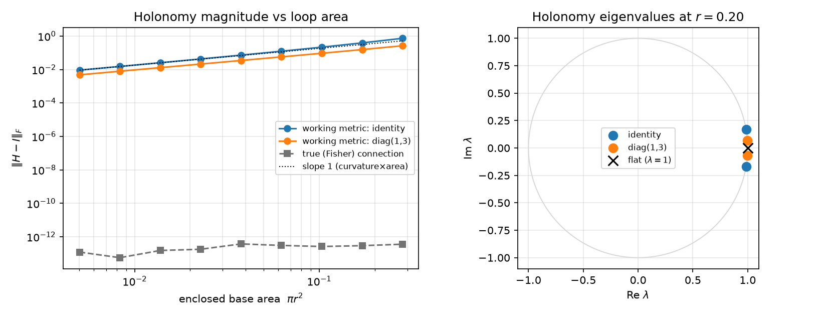
This matters because every practical sampler uses a fixed metric. NUTS adapts a mass matrix once during warmup and then holds it; a blocked sampler uses whatever conditional scale it is handed. Such a sampler does not transport along the flat true connection but along the curved \(A_M\) of its own working metric, so it can experience a genuine algorithmic holonomy (a systematic, orientation- and area-dependent fiber drift after the hyperparameters traverse a loop) even though the underlying geometry is flat. This reframes the empirical signal of Section 4: the loop-conditional dependence \(\hat{\rho}_j\) is an algorithmic, not geometric, footprint, and the attribution test (Section 4.7) asks precisely whether it carries the orientation and area structure that holonomy would imply. For NUTS on the GLMM it does not, which is consistent with NUTS adapting a metric close enough to horizontal that \(A_M\) has little curvature in the explored region. A deliberately mis-scaled sampler should instead show algorithmic holonomy tracking the curvature of its working metric — a concrete, testable prediction. This is the subject of a companion paper: a horizontal leapfrog HMC sampler that recomputes \(A\) at every leapfrog step so that trajectories follow horizontal lifts, keeping the working metric aligned with \(-\partial^2_{\boldsymbol{\alpha}}\ell\) so that \(A_M\) stays flat. That paper develops the full treatment: ergodicity arguments, the Metropolis–Hastings correction, a compiled backend, and multi-model benchmarks against NUTS on coupling-dominated targets.
This closes the loop with the hypothesis we set out to test. For the geometric program in MCMC, the Riemannian and connection-aware samplers that would naturally pursue a curvature account of centring, the flat result is a redirection rather than a dead end: there is no base–fiber holonomy to transport along in a hierarchical posterior, so the effort is better spent keeping a sampler’s working metric aligned with the true Hessian, which is where the exploitable curvature lives.
9.3 Limitations and future work↩︎
9.3.0.1 Model-specific derivations.
The flatness itself is not model-specific (Proposition 1); only the closed-form connection, curvature, and prior fraction of Section 5 are particular to the logistic GLMM. For other models the same quantities follow from \(G_{FF}\) and \(G_{BF}\), which can be obtained by reverse-mode automatic differentiation of the log-posterior gradient; supplying them is the natural next step for a compiled backend, and the prior fraction \(\pi_j = (\partial^2_{\alpha_j}\text{prior})/G_{FF,j}\) generalises directly.
9.3.0.2 Simulation study.
The simulation study uses a single model family and does not include a power analysis for the dependence diagnostic. Characterising the minimum detectable signal as a function of chain length and number of groups is an important practical question left for future work.
9.3.0.3 Fiber degeneracy.
A second failure mode, distinct from residualisation leakage, arises when the fiber itself has collapsed under the funnel pathology. The diagnostic estimates per-group dependence coefficients from residual fiber variation around detected loops; if the fiber has contracted to near a point, as happens when an unidentified group-level parameter is pinned close to its prior mean under a tight prior and near-absent likelihood, there is no variance to autocorrelate and \(\hat{\rho}_j \to 0\) regardless of pathology severity. The diagnostic is therefore blindest in the most severe cases: a collapsed fiber and a well-mixed fiber are observationally equivalent in \(\hat{\rho}_j\). This was observed in a spike-and-slab changepoint model where some subjects’ second changepoint parameter was completely unidentified; those subjects produced \(\hat{\rho}_j \approx 0\) despite sitting in a Neal funnel, while the analytic prior fraction \(\pi_j\) correctly flagged the group. The two failure modes — residualisation leakage (Section 4.7), which inflates \(\hat{\rho}_j\) at short gaps, and fiber degeneracy, which suppresses it in collapsed groups — act in opposite directions and should both be considered when interpreting a low \(\hat{\rho}_j\). The analytic \(\pi_j\), which depends only on the model structure and pilot draws rather than on chain variation, is the more robust per-group flag and should be treated as the primary output.
9.3.0.4 Prior dependence of \(\pi_j\).
We compute \(\pi_j\) at a point estimate of \(\sigma\), so it inherits the \(\sigma\)-hyperprior when \(\sigma\) is weakly identified (few groups). Reporting \(\pi_j\) per posterior draw, its distribution rather than a plug-in value, propagates this uncertainty, and a wide posterior for \(\pi_j\) is itself the signal that a group’s reading is hyperprior-sensitive. This refinement is natural future work.
9.3.0.5 Variational inference.
The same geometric structure applies to variational families: the fibration of the space of variational parameters over the mean-field components has a connection whose curvature determines the holonomy of the variational update. This connection to variational Bayes geometry is speculative but worth pursuing.
9.4 Note on methods of discovery↩︎
This work was developed through an extended, iterative collaboration with Claude Sonnet (Anthropic). The fiber bundle framing, the mathematical derivations, the R package architecture, and the exposition were developed jointly through dialogue rather
than by the author alone. The mathematical results were checked both analytically and numerically (the package test suite and data-raw/verify_flat_connection.R); the flatness result in particular emerged from a critical re-examination of an
earlier draft that had reported only the linearised curvature. The scientific framing, experimental decisions, and responsibility for errors are the author’s. The author views this as an example of AI-collaborative mathematical research, distinct from
using AI as a writing assistant or code generator, and reports it explicitly rather than subsuming it into generic tool-use language, in the hope that transparent description contributes to evolving community norms around human–AI co-production of
scientific knowledge.
Acknowledgements↩︎
Computations were performed using Stan [24] via cmdstanr [23], and the posterior package [22].
References↩︎
Code and package available at https://github.com/ABindoff/fibr.↩︎