Beyond-Third-Order Quantum Coherence in Two-Dimensional Spectroscopy via Order-Selective Isolation
June 11, 2026
A central challenge in nonlinear spectroscopy is the order-selective readout of weak higher-order responses that spectrally overlap with dominant lower-order signals. This bottleneck is particularly severe in two-dimensional (2D) spectroscopy, where extending conventional phase-cycling schemes to higher orders rapidly increases measurement and analysis complexity. Here we introduce a computation-assisted strategy that combines rotating-frame acquisition with a frame-shift tracking algorithm to separate signals by their frame-dependent spectral shifts. In a rubidium vapor experiment, we use this approach to isolate a 7th-order nonlinear contribution from coexisting 3rd-order components, enabling direct access to higher-order quantum-coherence dynamics without sacrificing operation at comparatively high pulse intensities. The method is broadly compatible with multidimensional spectroscopy platforms and provides a practical route to probing many-body and collective ultrafast dynamics beyond third order.
1 Introduction↩︎
A longstanding challenge in nonlinear spectroscopy is to increase the signal-to-noise ratio while retaining order-selective identification of dynamical components. In the weak-field regime, linear absorption and third-order pump–probe signals are often sufficient to describe the response [1]–[3]. At higher excitation, however, additional nonlinear orders emerge and overlap spectrally, obscuring the interpretation of pathways linked to collective excitations and many-body interactions. This trade-off between sensitivity and order specificity is a major bottleneck for pushing multidimensional spectroscopy toward probing higher-order and many-body nonlinear responses.
Two-dimensional (2D) spectroscopy [4]–[10] has enabled the isolation of third-order responses through coherent-control strategies, non-collinear geometries separate pathways via phase matching [4], [11], [12], while collinear implementations use phase cycling to disentangle selected quantum pathways [6], [13], [14]. Yet, when higher-order contributions must be resolved or removed, these approaches typically demand substantially larger phase-cycling steps and heavier post-processing, leading to rapidly growing experimental and computational complexity.
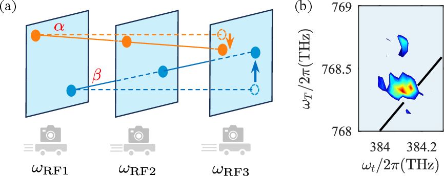
Figure 1: Scheme of the Frame-shift tracking separation algorithm for two-dimensional spectroscopy and the sorted 7-th signals.(a) The scheme for the separation. Three spectra are sampled under different rotation frame frequency \(\omega_{\mathrm{RF}}\), resembling the reduction of relative speed in a moving frame with constant velocity in classical mechanics. Movement of the spectral features (blue and orange points) is created with different slopes \(k_{\alpha}=-1\) and \(k_{\beta}=3\)for the frequency shift \(\omega_{T}^{\mathrm{eff}}\) of the 3rd- and7th-order signals, respectively. (b) The experimentally sorted 7th-order signals for rubidium vapor. The signal is sorted out by tracking the movement of the orange peak in subfigure (a) with the frame-shift tracking algorithm..
Recently, computation-assisted methods have emerged as a powerful alternative to this limitation [15]–[17]. These methods introduce controlled modulations of experimental parameters that generate order-dependent responses, followed by algorithmic separation. For example, intensity cycling in pump–probe measurements exploits nonlinear power scaling to allow disentangling mixed signal components [16]. Such strategies relax intensity constraints while preserving interpretability, and therefore offer a promising route to high-order multidimensional spectroscopy.
Building on this computation-assisted framework, we combine rotating-frame 2D measurements with a frame-shift tracking analysis that extracts order-dependent peak-shift slopes across multiple rotating frequencies. We experimentally validate the method in a rubidium vapor cell [18], [19]. As shown in Fig. 1 (a), the rotating-frame frequency \(\omega_{\mathrm{RF}}\) induces systematic displacements in the effective spectral coordinate \(\omega_{T}^{\mathrm{eff}}\). Tracking these displacements identifies distinct slope classes (lines \(\alpha\) and \(\beta\)), which directly encode nonlinear order. Using this criterion, we isolate a seventh-order contribution [Fig. 1 (b)] from overlapping lower-order backgrounds. Importantly, the separation remains effective at pulse intensities where higher-order signals are experimentally accessible, enabling practical access to beyond-third-order coherence dynamics.
2 Theory for Designing Computation-Assisted Spectroscopy↩︎
2.1 Pump–Probe Configuration and Measured Signal Formulation↩︎
Our current setup for the two-dimensional spectroscopy is under the pump-probe geometry, where two pump pulses, generated by a pulse shaper, are collinear with their wave vectors as \(\mathbf{k}_{1}\) and \(\mathbf{k}_{1'}\) (\(\mathbf{k}_{1'}=\mathbf{k}_{1}\)), and the probe pulse propagates in a non-collinear direction \(\mathbf{k}_{2}\). Here we focus on a modified pulse sequence where the probe pulse is designed to arrive first at the sample with the time intervals between the three pulses denoted as \(\tau\) and \(T\), as illustrated in Fig. 2 (a). The detection is along the direction of the probe pulse with signal \(E_{s}(\tau,T,\omega_{t})\), where \(\omega_{t}\) is the frequency of the signal, obtained directly via a spectrometer. Such a sequence allows the investigation of double-quantum (2Q) coherence [18], [20]–[23] between the doubly excited state and the ground state within the time interval \(T\) .
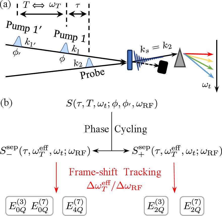
In this sequence, the probe pulse also serves as the local oscillator (LO). The signal is emitted only upon the arrival of the second pump pulse. The signal field lags behind the probe pulse by a time interval of \(\tau+T\), resulting in an additional phase accumulation \(\exp[-i\omega_{t}(\tau+T)]\) during the propagation of the probe pulse. The measured signal consequently takes the form, \[\begin{align} & & S(\tau,T,\omega_{t};\phi,\phi',\omega_{\mathrm{RF}})\nonumber \\ & \approx & 2\text{Re}[E_{s}(\tau,T,\omega_{t};\phi,\phi',\omega_{\mathrm{RF}})E_{2}^{*}(\omega_{t})e^{i\omega_{t}(\tau+T)}],\label{eq:signal} \end{align}\tag{1}\] where \(E_{2}(\omega_{t})\) represents the field of the probe pulse, and \(\phi\) (\(\phi'\)) denotes the phase of the first (second) pump pulse. The multi-quantum 2D spectroscopy \(S(\tau,\omega_{T},\omega_{t};\phi,\phi',\omega_{\mathrm{RF}})\) is obtained by sampling and Fourier transform of \(S(\tau,T,\omega_{t};\phi,\phi',\omega_{\mathrm{RF}})\) with respect to the time variable \(T\).In the signal-processing procedure of the double-quantum spectroscopy framework, a causality enforcement condition is additionally applied to preserve the causal ordering of the emitted signal field, which is a standard treatment in multidimensional coherent spectroscopy [8], [22].
The present experimental design employs relatively strong excitation pulses, giving rise to signals that contain significant contributions beyond the typical third order. The signal \(E_{s}(\tau,T,\)
\(\omega_{t};\phi,\phi',\omega_{\mathrm{RF}})\) along the probe direction ( i.e., \(\mathbf{k}_{s}=\mathbf{k}_{2}\)) can be decomposed into different components as \(E_{s}(\tau,T,\omega_{t};\phi,\phi',\omega_{\mathrm{RF}})=\sum_{n}E_{s}^{(2n+1)}(\tau,T,\omega_{t};\phi,\phi',\omega_{\mathrm{RF}})\) of the \((2n+1)\)th order as \(\mathbf{k}_{s}=\mathbf{k}_{2}+n_{1}\mathbf{k}_{1}-m_{1}\mathbf{k}_{1}+n_{2}\mathbf{k}_{1'}-m_{2}\mathbf{k}_{1'}\), where \(n_{1}+m_{1}+n_{2}+m_{2}=2n\), \(n=1,2,3,\cdots\) with \(n_{1}-m_{1}+n_{2}-m_{2}=0\). We define the configurations satisfying \((n_{1},m_{1},n_{2},m_{2})=(n,0,0,n)\) or \((0,n,n,0)\) as fully symmetric configurations, while all remaining cases are referred to as asymmetric configurations.
These \((2n+1)\)th-order components result from different combinations of \(2n\) interactions with the two collinear pump pulses \(\mathbf{k}_{1}\) and \(\mathbf{k}_{1'}\), while the probe pulse is assumed to be sufficiently weak to interact only once with the sample. In the excitation situations governed by the phase-matching condition, the sign of a wave vector is directly related to the change of excitation numbers in the density matrix element \(\rho_{\alpha,\alpha'}\), where \(\left|\alpha\right\rangle\) and \(\left|\alpha'\right\rangle\) are the eigen-states of the system Hamiltonian. A positive wave vector (e.g., \(+\mathbf{k}_{1}\)) increases the excitation number \(\alpha\) or decreases \(\alpha\prime\), while a negative wave vector (e.g., \(-\mathbf{k}_{1}\)) decreases \(\alpha\) or increases \(\alpha\prime\). The measured signal arises from different \(M\)-th quantum coherences within the time interval \(T\), which correspond to density matrix elements \(\rho_{n_{1}+1,m_{1}}\) with the coherence order \(M=\left|n_{1}+1-m_{1}\right|\), indicating the absolute difference in the number of excitations between the two states \(\left|n_{1}+1\right\rangle\) and \(\left|m\right\rangle\). Critically, under strong pump fields, a given multi-quantum coherence signal (e.g., 2Q) during \(T\) comprises contributions from multiple nonlinear orders.
2.2 Fully Symmetric Configuration and Coherence Separation Strategy↩︎
In this letter, we first and primarily focus on two types of fully symmetric \((2n+1)\)th-order signals, (i) with the phase-matching condition \(\mathbf{k}_{s}=\mathbf{k}_{2}+n\mathbf{k}_{1}-n\mathbf{k}_{1'}\) i.e., \(n_{1}=m_{2}=n\) and \(m_{1}=n_{2}=0\), which induces the highest-order coherence \(\rho_{n+1,0}\) with \(M=n+1\), i.e., and (ii) with \(\mathbf{k}_{s}=\mathbf{k}_{2}-n\mathbf{k}_{1}+n\mathbf{k}_{1'}\) (\(n_{1}=m_{2}=0\) and \(m_{1}=n_{2}=n\)) which results in the second-highest coherence \(\rho_{1,n}\) and \(\rho_{0,n-1}\) with \(M=n-1\), during the delay time \(T\). The corresponding signal fields are denoted as \(E_{(n+1)Q}^{(2n+1)}(\tau,T,\omega_{t};\phi,\phi',\omega_{\mathrm{RF}})\) and \(E_{(n-1)Q}^{(2n+1)}(\tau,T,\omega_{t};\phi,\phi',\omega_{\mathrm{RF}})\), respectively. We note here that any signal with coherence on the order \(M=n\) is cycled out in the subsequent signal processing via phase cycling. Based on this fully symmetric configuration, which supports the generation of both the highest-order and second-highest-order coherences, we develop the corresponding separation scheme. The remaining configurations are discussed in detail in the following section, where we take the seventh-order signal as a representative example for a comprehensive analysis.
The overall signal separation proceeds through two key steps: First, phase cycling separates the acquired signal into two distinct spectra. Then, by combining a rotating-frame scheme with a frame-shift tracking algorithm, high-order signal components are identified and isolated, as illustrated in Fig. 2(b). We now elaborate on these two core procedures as follows.
In our partially collinear geometry, \((n-1)Q\) and \((n+1)Q\) signal fields exhibit phase dependencies, \[E_{(n+1)Q}^{(2n+1)}(\tau,T,\omega_{t};\phi,\phi',\omega_{\mathrm{RF}})\propto\text{exp[in(\phi-\phi')]},\label{eq:n431}\tag{2}\] \[E_{(n-1)Q}^{(2n+1)}(\tau,T,\omega_{t};\phi,\phi',\omega_{\mathrm{RF}})\propto\text{exp[in(-\phi+\phi')].}\label{eq:n-1}\tag{3}\] In our protocol, we implement a four-step phase cycle: \(\Phi_{1}=(\phi=0,\phi'=0)\), \(\Phi_{2}=(\phi=0,\phi'=\pi/2)\), \(\Phi_{3}=(\phi=0,\phi'=\pi)\),and \(\Phi_{4}=(\phi=0,\phi'=3\pi/2)\). The measured signals are combined into \(S_{+}^{\mathrm{sep}}(\tau,T,\omega_{t};\omega_{\mathrm{RF}})=S(\tau,T,\omega_{t};0,0,\omega_{\mathrm{RF}})+iS(\tau,T,\omega_{t};0,\pi/2,\omega_{\mathrm{RF}})\) and \(S_{-}^{\mathrm{sep}}(\tau,T,\omega_{t};\omega_{\mathrm{RF}})=S(\tau,T,\omega_{t};0,0,\omega_{\mathrm{RF}})-iS(\tau,T,\omega_{t};0,\pi/2,\omega_{\mathrm{RF}})\), where \(S(\tau,T,\omega_{t};0,0,\)
\(\omega_{\mathrm{RF}})=S^{0}(\tau,T,\omega_{t};0,0,\omega_{\mathrm{RF}})-S^{0}(\tau,T,\omega_{t};0,\pi,\omega_{\mathrm{RF}})\), and \(S(\tau,T,\omega_{t};0,\pi/2,\omega_{\mathrm{RF}})=S^{0}(\tau,T,\)
\(\omega_{t};0,\pi/2,\omega_{\mathrm{RF}})-S^{0}(\tau,T,\omega_{t};0,3\pi/2,\omega_{\mathrm{RF}})\), with \(S^{0}\) denoting the raw experimentally acquired signals. Such phase cycling
eliminates transient absorption signal [9], and also helps to isolate different coherences [8] as follows. Signals with even \(n\) (e.g., fifth-order with \(n=2\)) are completely suppressed, while signals with odd \(n\) are separated into \(S_{+}^{\mathrm{sep}}(\tau,T,\omega_{t};\omega_{\mathrm{RF}})\) and \(S_{-}^{\mathrm{sep}}(\tau,T,\omega_{t};\omega_{\mathrm{RF}})\)
depending on \(n\): for \(n=1,5,9,\cdots\), the \((n+1)Q\) contributions appear in \(S_{+}^{\mathrm{sep}}(\tau,T,\omega_{t};\omega_{\mathrm{RF}})\), whereas the \((n-1)Q\) contributions appear in \(S_{-}^{\mathrm{sep}}(\tau,T,\omega_{t};\omega_{\mathrm{RF}})\); for \(n=3,7,11,\cdots\), the \((n-1)Q\) contributions appear in \(S_{+}^{\mathrm{sep}}(\tau,T,\omega_{t};\omega_{\mathrm{RF}})\), whereas the \((n+1)Q\) contributions appear in \(S_{-}^{\mathrm{sep}}(\tau,T,\omega_{t};\omega_{\mathrm{RF}})\). For example, the \(E_{2Q}^{(7)}\) and \(E_{2Q}^{(3)}\) are isolated into \(S_{+}^{\mathrm{sep}}(\tau,T,\omega_{t};\omega_{\mathrm{RF}})\), while the \(E_{4Q}^{(7)}\) and \(E_{0Q}^{(3)}\) are isolated into \(S_{-}^{\mathrm{sep}}(\tau,T,\omega_{t};\omega_{\mathrm{RF}})\).
Next, we develop a new method based on the rotating frame to further isolate different signals in \(S_{+}^{\mathrm{sep}}(\tau,T,\omega_{t};\omega_{\mathrm{RF}})\) and \(S_{-}^{\mathrm{sep}}(\tau,T,\omega_{t};\omega_{\mathrm{RF}})\) spectra. To reduce the sampling rate, a rotating frame with frequency \(\omega_{\mathrm{RF}}\) is applied to the first pump pulse via a pulse shaper, which modifies the temporal oscillations of the \((2n+1)\)th-order signal fields during \(T\) as follows: \[\begin{align} E_{(n+1)Q}^{(2n+1)}(\tau,T,\omega_{t};\omega_{\mathrm{RF}}) & \propto & \exp[-i(\omega_{n+1,0}-n\omega_{\mathrm{RF}})T], \end{align}\] and \[\begin{align} E_{(n-1)Q}^{(2n+1)}(\tau,T,\omega_{t};\omega_{\mathrm{RF}}) & \propto & \exp[-i(-\omega_{n,1}+n\omega_{\mathrm{RF}})T]\\ & \mathrm{or} & \exp[-i(-\omega_{n-1,0}+n\omega_{\mathrm{RF}})T],\nonumber \end{align}\] where \(\omega_{\alpha,\alpha'}\equiv\omega_{\alpha}-\omega_{\alpha'}\) is the energy gap between the energy levels with \(\alpha\) and \(\alpha'\) of the density matrix \(\rho_{\alpha,\alpha'}\). Incorporating the propagation phase factor \(\exp[-i\omega_{t}(\tau+T)]\) in Eq. (1 ), we derive the effective oscillation frequency \(\omega_{T}^{\text{eff}}\) that appear in the Fourier transform spectra \(S_{\pm}^{\mathrm{sep}}(\tau,\omega_{T}^{\text{eff}},\omega_{t};\omega_{\mathrm{RF}})\) as \(\omega_{T}^{\text{eff}}=\omega_{n+1,0}-n\omega_{\mathrm{RF}}-\omega_{t}\) for the \((n+1)Q\) signals and \(\omega_{T}^{\text{eff}}=-\omega_{n,1}+n\omega_{\mathrm{RF}}-\omega_{t}\) for the \((n-1)Q\) signals. The shift rate of spectral peaks along the \(\omega_{T}^{\text{eff}}\) axis with respect to \(\omega_{\mathrm{RF}}\), \(\Delta\omega_{T}^{\text{eff}}/\Delta\omega_{\mathrm{RF}}\), provides an intrinsic signature of the nonlinear order. Such a rate difference \(\Delta\omega_{T}^{\text{eff}}/\Delta\omega_{\mathrm{RF}}=\pm n\) between the \((n+1)Q\) and \((n-1)Q\) signal allows for both the separation and unambiguous identification of signal components.
2.3 General Behavior of High-Order Pathways: A Seventh-Order Analysis↩︎
To comprehensively model the isolation of high-order signals, we must account for all nonlinear processes that induce signals along the phase-matching direction \(\mathbf{k}_{s}=\mathbf{k}_{2}\). We therefore adopt the general expression for the signal wave vectors as defined earlier: \(\mathbf{k}_{s}=\mathbf{k}_{2}+n_{1}\mathbf{k}_{1}-m_{1}\mathbf{k}_{1}+n_{2}\mathbf{k}_{1'}-m_{2}\mathbf{k}_{1'}\), where \(\mathbf{k}_{1}=\mathbf{k}_{1'}\). Under this model, the phase-matching condition is satisfied with \(n_{1}+n_{2}=m_{1}+m_{2}\).
To illustrate all the possible pathways related to the current discussion, we divide the pathways for the signals on the \((2n+1)\)th-order into two scenarios, (1) \(n_{1}+m_{1}=n_{2}+m_{2}=n\); (2) \(n_{1}+m_{1}\neq n_{2}+m_{2}\). To clearly demonstrate the properties of these pathways, we take an example for the 7-th order with \(n=3\). We mainly focus on the resulting coherence types, which relate to the frequency \(\omega_{T}\).
1pt
| Situation | Signal Direction \(\mathbf{k}_{s}\) | Coherence Type | Effective Frequency \(\omega_{T}^{\text{eff}}\) | \(\frac{\Delta\omega_{T}^{\text{eff}}}{\Delta\omega_{\mathrm{RF}}}\) | Assigned Spectrum | Separation Scheme | ||
|---|---|---|---|---|---|---|---|---|
| 1 | \(\mathbf{k}_{2}+3\mathbf{k}_{1}-3\mathbf{k}_{1'}\) | \(\rho_{4,0}\)(4Q) | \(\omega_{4,0}-3\omega_{\mathrm{RF}}-\omega_{t}\) | -3 | \(S_{-}^{\mathrm{sep}}\) | Velocity-resolved | ||
| 2 | \(\mathbf{k}_{2}-3\mathbf{k}_{1}+3\mathbf{k}_{1'}\) | \(\rho_{3,1}\)(2Q) | \(-\omega_{3,1}+3\omega_{\mathrm{RF}}-\omega_{t}\) | +3 | \(S_{+}^{\mathrm{sep}}\) | Velocity-resolved | ||
| 3 | \(\rho_{2,0}\)(2Q) | \(-\omega_{2,0}+3\omega_{\mathrm{RF}}-\omega_{t}\) | +3 | |||||
| 4 | \(\mathbf{k}_{2}+2\mathbf{k}_{1}-\mathbf{k}_{1}-2\mathbf{k}_{1'}+\mathbf{k}_{1'}\) | \(\rho_{3,1}\)(2Q) | \(\omega_{3,1}-\omega_{\mathrm{RF}}-\omega_{t}\) | -1 | \(S_{+}^{\mathrm{sep}}\) | Degenerate (with 3rd) | ||
| 5 | \(\rho_{2,0}\)(2Q) | \(\omega_{2,0}-\omega_{\mathrm{RF}}-\omega_{t}\) | -1 | |||||
| 6 | \(\mathbf{k}_{2}+\mathbf{k}_{1}-2\mathbf{k}_{1}-\mathbf{k}_{1'}+2\mathbf{k}_{1'}\) | \(\rho_{2,2}\)(0Q) | \(-\omega_{2,2}+\omega_{\mathrm{RF}}-\omega_{t}\) | +1 | \(S_{-}^{\mathrm{sep}}\) | Frequency-resolved | ||
| 7 | \(\rho_{1,1}\)(0Q) | \(-\omega_{1,1}+\omega_{\mathrm{RF}}-\omega_{t}\) | +1 | Degenerate (with 3rd) | ||||
| 8 | \(\rho_{0,0}\)(0Q) | \(-\omega_{0,0}+\omega_{\mathrm{RF}}-\omega_{t}\) | +1 | Degenerate (with 3rd) | ||||
| 9 | \(\mathbf{k}_{2}+\mathbf{k}_{1}-3\mathbf{k}_{1'}+2\mathbf{k}_{1'}\) | \(\rho_{2,0}\)(2Q) | \(\omega_{2,0}-\omega_{\mathrm{RF}}-\omega_{t}\) | -1 | \(S_{+}^{\mathrm{sep}}\) | Degenerate (with 3rd) | ||
| 10 | \(\mathbf{k}_{2}-\mathbf{k}_{1}+3\mathbf{k}_{1'}-2\mathbf{k}_{1'}\) | \(\rho_{1,1}\)(0Q) | \(-\omega_{1,1}+\omega_{\mathrm{RF}}-\omega_{t}\) | +1 | \(S_{-}^{\mathrm{sep}}\) | Degenerate (with 3rd) | ||
| 11 | \(\rho_{0,0}\)(0Q) | \(-\omega_{0,0}+\omega_{\mathrm{RF}}-\omega_{t}\) | +1 | |||||
| 12 | \(\mathbf{k}_{2}+3\mathbf{k}_{1}-2\mathbf{k}_{1}-\mathbf{k}_{1'}\) | \(\rho_{4,2}\)(2Q) | \(\omega_{4,2}-\omega_{\mathrm{RF}}-\omega_{t}\) | -1 | \(S_{+}^{\mathrm{sep}}\) | Frequency-resolved | ||
| 13 | \(\rho_{3,1}\)(2Q) | \(\omega_{3,1}-\omega_{\mathrm{RF}}-\omega_{t}\) | -1 | Frequency-resolved | ||||
| 14 | \(\rho_{2,0}\)(2Q) | \(\omega_{2,0}-\omega_{\mathrm{RF}}-\omega_{t}\) | -1 | Degenerate (with 3rd) | ||||
| 15 | \(\mathbf{k}_{2}+2\mathbf{k}_{1}-3\mathbf{k}_{1}+\mathbf{k}_{1'}\) | \(\rho_{3,3}\)(0Q) | \(-\omega_{3,3}+\omega_{\mathrm{RF}}-\omega_{t}\) | +1 | \(S_{-}^{\mathrm{sep}}\) | Frequency-resolved | ||
| 16 | \(\rho_{2,2}\)(0Q) | \(-\omega_{2,2}+\omega_{\mathrm{RF}}-\omega_{t}\) | +1 | Degenerate (with 3rd | ||||
| or case 6) | ||||||||
| 17 | \(\rho_{1,1}\)(0Q) | \(-\omega_{1,1}+\omega_{\mathrm{RF}}-\omega_{t}\) | +1 | Degenerate (with 3rd) | ||||
| 18 | \(\rho_{0,0}\)(0Q) | \(-\omega_{0,0}+\omega_{\mathrm{RF}}-\omega_{t}\) | +1 | Degenerate (with 3rd) | ||||
| 19 | \(\mathbf{k}_{2}+3\mathbf{k}_{1}-\mathbf{k}_{1}-2\mathbf{k}_{1'}\), \(\mathbf{k}_{2}+2\mathbf{k}_{1}-3\mathbf{k}_{1'}+\mathbf{k}_{1'}\) | 3Q | — | — | — | Phase-cycled out | ||
| 20 | \(\mathbf{k}_{2}-3\mathbf{k}_{1}+\mathbf{k}_{1}+2\mathbf{k}_{1'}\), \(\mathbf{k}_{2}-2\mathbf{k}_{1}+3\mathbf{k}_{1'}-\mathbf{k}_{1'}\) | 1Q | — | — | — | Phase-cycled out | ||
| 21 | \(\mathbf{k}_{2}+2\mathbf{k}_{1}-2\mathbf{k}_{1}+\mathbf{k}_{1'}-\mathbf{k}_{1'}\), \(\mathbf{k}_{2}+\mathbf{k}_{1}-\mathbf{k}_{1}+2\mathbf{k}_{1'}-2\mathbf{k}_{1'}\) | 1Q | — | — | — | Phase-cycled out | ||
Scenario (1) with \(n_{1}+m_{1}=n_{2}+m_{2}=3\). In this scenario, the first case is \((n_{1}=m_{2}=3\), \(m_{1}=n_{2}=0)\) and \((m_{1}=n_{2}=3\), \(n_{1}=m_{2}=0)\), corresponding to the phase matching conditions \(\mathbf{k}_{s}=\mathbf{k}_{2}+3\mathbf{k}_{1}-3\mathbf{k}_{1'}\) and \(\mathbf{k}_{s}=\mathbf{k}_{2}-3\mathbf{k}_{1}+3\mathbf{k}_{1'}\). These pathways belong to the fully symmetric excitation configuration introduced in the previous subsection, and presented as lines 1 - 3 in the Table. ¿tbl:table195em?. As discussed in the previous subsection, the fully symmetric configuration constitutes the central design principle of our separation framework, since it directly generates the highest- and second-highest-order coherences with well-defined rotating-frame shift rates. For the second phase-matching condition, a distinct coherence \(\rho_{3,1}\) emerges with oscillation frequency \(\omega_{3,1}\). This frequency arises from multi-atom interactions and corresponds to a distinct spectral position, as indicated in line 2 of the Table. ¿tbl:table195em?. However, due to potentially weak interaction strengths or minute energy-level shifts, the corresponding signal may be too weak to be discernible in our spectra. We note this possibility for reference, though it does not manifest as a distinct feature in our current measurements.In the following discussion, we further extend the analysis to asymmetric excitation configurations and examine their corresponding spectral behaviors within the same theoretical framework.
The second case includes two phase matching conditions, \(\mathbf{k}_{s}=\mathbf{k}_{2}+2\mathbf{k}_{1}-\mathbf{k}_{1}+\mathbf{k}_{1'}-2\mathbf{k}_{1'}\) and \(\mathbf{k}_{s}=\mathbf{k}_{2}+\mathbf{k}_{1}-2\mathbf{k}_{1}+2\mathbf{k}_{1'}-1\mathbf{k}_{1'}\). For the first phase matching condition, the second pulse, interacting with the system three times, results in the coherence \(\rho_{3,1}\) or \(\rho_{2,0}\) during the waiting time \(T\). For the signal related to coherence \(\rho_{2,0}\) (line 5 in Table. ¿tbl:table195em?), the oscillation frequency \(\omega_{T}=\omega_{2,0}\) is exactly the same as that created by the third order response along the phase matching condition \(\mathbf{k}_{s}=\mathbf{k}_{2}+\mathbf{k}_{1}-\mathbf{k}_{1'}\). Such a signal cannot be separated with the current method, yet may be distinguished with the power cycling in Ref. [16]. We also would like to remark that the isolation of these types of high-order signals will not provide any additional information due to the exact dynamics. And we name this type of high-order signal as the “shielding” effect on the low-order signal. The signal related to the coherence \(\rho_{3,1}\) (line 4 in Table. ¿tbl:table195em?) may have a different oscillation frequency \(\omega_{T}=\omega_{3,1}\), which may be different from the interaction between Rb atoms. Such a difference shall result in a different position on the 2D spectra. The second phase matching condition may also give rise to a different coherence \(\rho_{f,D_{2}+D_{2}}\) (line 6 in Table. ¿tbl:table195em?), where the state \(\left|f\right\rangle\) is the \(5^{2}S_{1/2}\leftrightarrow5^{2}D\) transition state created by the probe and pump pulse, and the state \(\left|D_{2}+D_{2}\right\rangle\) denotes a double \(D_{2}\) transition.
These observation lead to a general rule for higher-order signals, whenever the pump-probe pulses generate higher-oder signals with the same dynamics as lower-order signal, these signals cannot be distinguished by the current methods. These shielding signals may not provide additional information, and shall not require extra effort to isolate them.
Scenario (2) with \(n_{1}+m_{1}\neq n_{2}+m_{2}\). This scenario includes four cases: (\(n_{1}+m_{1}=1,n_{2}+m_{2}=5\)), (\(n_{1}+m_{1}=2,n_{2}+m_{2}=4\)), (\(n_{1}+m_{1}=4,n_{2}+m_{2}=2\)), and (\(n_{1}+m_{1}=5,n_{2}+m_{2}=1\)). The cases (\(n_{1}+m_{1}=2,n_{2}+m_{2}=4\)) and (\(n_{1}+m_{1}=4,n_{2}+m_{2}=2\)) resemble the even \(n\) situation and are canceled by phase-cycling procedure; they correspond to lines 19, 20, and 21 in Table. ¿tbl:table195em?, respectively.
For the remaining cases (\(n_{1}+m_{1}=1,n_{2}+m_{2}=5\)) and (\(n_{1}+m_{1}=5,n_{2}+m_{2}=1\)), the first case (\(n_{1}+m_{1}=1,n_{2}+m_{2}=5\)) includes two phase matching conditions, \(\mathbf{k}_{s}=\mathbf{k}_{2}+\mathbf{k}_{1}-3\mathbf{k}_{1'}+2\mathbf{k}_{1'}\) and \(\mathbf{k}_{s}=\mathbf{k}_{2}-\mathbf{k}_{1}+3\mathbf{k}_{1'}-2\mathbf{k}_{1'}\), in which the second pulse interacts once with the system. For the first phase matching condition, the second pulse generates the coherence \(\rho_{2,0}\) (line 9 in Table. ¿tbl:table195em?) during the waiting time \(T\), oscillating at \(\omega_{T}=\omega_{2,0}\). This frequency is identical to that produced by the 3rd-order signal with \(\mathbf{k}_{s}=\mathbf{k}_{2}+\mathbf{k}_{1}-\mathbf{k}_{1'}\), and therefore cannot be separated. For the second phase matching condition, the coherence is either \(\rho_{1,1}\) (line 10 in Table. ¿tbl:table195em?) or \(\rho_{0,0}\) (line 11 in Table. ¿tbl:table195em?), oscillating at \(\omega_{1,1}\) or \(\omega_{0,0}\), which likewise coincides with the third order signal along \(\mathbf{k}_{s}=\mathbf{k}_{2}-\mathbf{k}_{1}+\mathbf{k}_{1'}\); hence it also cannot be separated.
The second case (\(n_{1}+m_{1}=5,n_{2}+m_{2}=1\)) also includes two phase matching conditions, \(\mathbf{k}_{s}=\mathbf{k}_{2}+3\mathbf{k}_{1}-2\mathbf{k}_{1}-\mathbf{k}_{1'}\) and \(\mathbf{k}_{s}=\mathbf{k}_{2}+2\mathbf{k}_{1}-3\mathbf{k}_{1}+\mathbf{k}_{1'}\), where the second pulse interacts with the system for five times. For the first phase matching condition, the second pulse yields coherence \(\rho_{4,2}\) (line 12 in Table. ¿tbl:table195em?), \(\rho_{3,1}\) (line 13 in Table. ¿tbl:table195em?), or \(\rho_{2,0}\) (line 14 in Table. ¿tbl:table195em?), oscillating at \(\omega_{4,2}\), \(\omega_{3,1}\), or \(\omega_{2,0}\). The signals oscillating at \(\omega_{4,2}\) and \(\omega_{3,1}\) arise from distinct atomic interactions and are thus expected to appear at different positions in the 2D spectra. In contrast, the component oscillating at \(\omega_{T}=\omega_{2,0}\) is degenerate with the third-order signal along \(\mathbf{k}_{s}=\mathbf{k}_{2}+\mathbf{k}_{1}-\mathbf{k}_{1'}\) and cannot be separated. For the second phase matching condition, the second pulse yields coherence \(\rho_{3,3}\) (line 15 in Table. ¿tbl:table195em?) \(\rho_{2,2}\) (line 16 in Table. ¿tbl:table195em?), \(\rho_{1,1}\) (line 17 in Table. ¿tbl:table195em?), or \(\rho_{0,0}\) (line 18 in Table. ¿tbl:table195em?), oscillating at \(\omega_{3,3}\), \(\omega_{2,2}\), \(\omega_{1,1}\), or \(\omega_{0,0}\).The frequency oscillating at \(\omega_{3,3}\) is also expected to be spectrally distinct. The component at \(\omega_{2,2}\) yields the same result as the line 6 in Table. ¿tbl:table195em? discussed above. Finally, the components at \(\omega_{1,1}\) and \(\omega_{0,0}\) are degenerate with the third order signal along \(\mathbf{k}_{s}=\mathbf{k}_{2}-\mathbf{k}_{1}+\mathbf{k}_{1'}\) and thus cannot be separated with current methods.
To conclude, a vast majority of signals not related to \(\mathbf{k}_{s}=\mathbf{k}_{2}\pm n\mathbf{k}_{1}\mp n\mathbf{k}_{1'}\), degenerate into lower-order signals, resulting in complete spectral overlap. This makes them intrinsically inseparable in our measurement. The remaining few special situations are readily identifiable through their dynamics, as exemplified by \(\mathbf{k}_{s}=\mathbf{k}_{2}+\mathbf{k}_{1}-2\mathbf{k}_{1}+2\mathbf{k}_{1'}-1\mathbf{k}_{1'}\).
2.4 Experimental Signal Extraction↩︎
To extract spectral shifts across different orders, we employ a frame-shift tracking algorithm, which is used in computer science to determine the position changes by comparing subsequent frame during the movement. Here, the movement of the spectra is created by changing the frequency \(\omega_{\mathrm{RF}}\) of the rotating frame. The procedure of our frame-shift tracking for spectra begins by applying an absolute threshold of 0.095 to the 2D spectra to suppress weak background signals. The remaining features are clustered to isolate distinct peaks. Each peak is then fitted with a two-dimensional Gaussian function to determine its center coordinates \((\omega_{x},\omega_{y})\)
\[S(\omega_{t},\omega_{T}^{\text{eff}})=a_{0}\exp[-\frac{(\omega_{t}-\omega_{x})^{2}}{\sigma_{x}^{2}}-\frac{(\omega_{T}^{\text{eff}}+\omega_{t}-\omega_{y})^{2}}{\sigma_{y}^{2}}]+b_{0},\label{eq:6}\tag{4}\] where \(a_{0}\) is the amplitude, \(\sigma_{x}\) and \(\sigma_{y}\) are the corresponding widths, and \(b_{0}\) is a constant background. The term \(\omega_{T}^{\text{eff}}+\omega_{t}\) captures the tilt of the signal induced by the phase factor \(\exp[i\omega_{t}(\tau+T)]\) in Eq. (1 ).
To track the displacement of peak centers \((\Delta\omega_{x},\Delta\omega_{y})\) between two rotating frames, we employ the Hungarian algorithm[24], [25], which solves the optimal assignment between peak sets by minimizing the total pairwise distance cost, similar to the algorithm of an optical mouse. This ensures robust and consistent peak matching as signals shift. The order of each signal is subsequently determined by comparing the observed relative shift \(\Delta\omega_{y}/\Delta\omega_{\mathrm{RF}}\) along the \(\omega_{T}^{\mathrm{eff}}\) axis, as shown in Fig. 1 (a) with the representative lines \(\alpha\) and \(\beta\). Further details of the tracking and isolation are presented later along with the experimental verification. We would remark that the current scheme with the rotating frame relies on differences in phase evolution or dynamics during the waiting time \(T\). When signals of different orders are fully degenerate in frequency and exhibit identical temporal evolution, they remain indistinguishable within the present framework.
3 Experimental verification↩︎
We validate this approach experimentally using a \(^{87}\mathrm{Rb}\) vapor system contained in a borosilicate cell filled with 450 Torr of nitrogen buffer gas to induce collisional broadening. The cell is stabilized at 120.0 °C (0.1 °C), yielding a high-density thermal vapor (approximately \(1.65\times 10^{13}\mathrm{cm}^{-3}\)).
Pump and probe pulses are generated by a Ti:Sapphire amplifier laser system producing pulses (800 nm, 30.8 fs) at a 1 kHz repetition rate. The central wavelength is tuned using an optical parametric amplifier (OPA), which allows spectral shifting to 382.9THz (783nm) for the present experiment.
The pump–probe excitation scheme is implemented using a pulse-shaping system consisting of an acousto-optic modulator (AOM), two parabolic mirrors, and a pair of gratings in a 4-f configuration. This setup converts a single pump pulse into two phase-controlled collinear pump pulses with a variable temporal separation T. The delay \(\tau\) between the probe pulse and the first pump pulse is controlled by a mechanical delay stage in the probe arm. Both pump and probe beams are focused onto the sample using a parabolic mirror to ensure optimal spatial overlap, and their polarizations are aligned horizontally using half-wave plates and polarizers prior to entering the sample.
The probe pulse after interaction with the sample is spectrally resolved using a spectrometer equipped with a charge-coupled device (CCD) camera. These pulses have a bandwidth (FWHM) of 11.9THz and spectrally cover the Rb \(D_{1}\) transition (\(377.1\text{THz}\), \(795\text{nm}\)), \(D_{2}\) transition (\(384.2\text{THz}\), \(780\text{nm}\)) and the excited state \(5^{2}P_{3/2}\leftrightarrow5^{2}D\) transition (\(386.3\text{THz}\), \(776\text{nm}\)) as shown in Fig. 3 (a). Experiments are conducted under three rotating-frame frequencies: \(380.9\text{THz}\) \((787\text{nm}\)), \(379.5\,\text{THz}\) (\(790\text{nm}\)), and \(378.05\text{THz}\) (\(793\text{nm}\)).
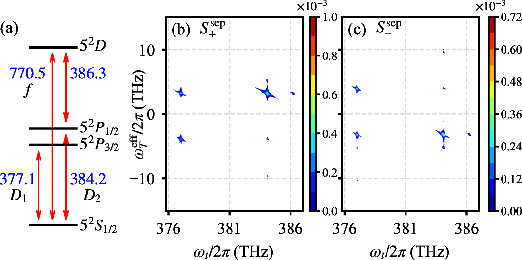
We apply the four-step phase cycling scheme with phase settings: \(\Phi_{1}\), \(\Phi_{2}\), \(\Phi_{3}\), and \(\Phi_{4}\). The separated spectra \(S_{+}^{\mathrm{sep}}(\tau,\omega_{T}^{\mathrm{eff}},\omega_{t};\omega_{\mathrm{RF}})\) and \(S_{-}^{\mathrm{sep}}(\tau,\omega_{T}^{\mathrm{eff}},\omega_{t};\omega_{\mathrm{RF}})\) of \(^{87}\textrm{Rb}\) atoms with different combination of measured data are shown in Figs. 3 (b) and (c), with the rotating frames \(\omega_{\mathrm{RF}}/2\pi=380.9\text{THz}\) (\(787\text{nm}\)). The emission frequencies of the signal are \(\omega_{t}/2\pi=377.1\text{THz}\), \(384.2\text{THz}\) and \(386.3\text{THz}\), corresponding to the frequencies of \(D_{1}\) transition, \(D_{2}\) transition and an excited state transition of an individual \(^{87}\mathrm{Rb}\) atom, respectively.
We first focus on the signal isolation for the spectrum \(S_{+}^{\mathrm{sep}}(\tau,\omega_{T}^{\mathrm{eff}},\omega_{t})\) in the following discussions. With the Gaussian fitting in Eq. (4 ), we identify 6 peaks, illustrated with the red circles in Fig. 4 (a), show the fitting results for the spectra \(S_{+}^{\mathrm{sep}}(\tau,\omega_{T}^{\mathrm{eff}},\omega_{t})\) with the rotating frame set at \(787\text{nm}\). With the same method, we also find the peak centers \((\omega_{x},\omega_{y})\) for the rotating frame at \(790\text{nm}\), illustrated as the blue points in Fig. 4 (b), along with the peak centers for \(787\mathrm{nm}\) as red points. Fig. 4 (b) clearly illustrates the different shift rates \(\Delta\omega_{T}^{\text{eff}}/\Delta\omega_{\mathrm{RF}}\) for peak centers.
Then we apply the Hungarian algorithm to determine the shift rates \(\Delta\omega_{T}^{\text{eff}}/\Delta\omega_{\mathrm{RF}}\) for all the 6 peaks with the results shown as blue pentagrams in Fig. 4 (c), where one peak has different rate \(\Delta\omega_{T}^{\text{eff}}/\Delta\omega_{\mathrm{RF}}=3\) from other 5 peaks cluster around a common value of \(-0.99 \pm 0.03\). With such differences, we will isolate the signal by introducing a mask functions for the \(i\)-th peak as \[\textrm{MF}_{i}(\omega_{t},\omega_{T}^{\mathrm{eff}})=\begin{cases} 1 & \textrm{if}\:d<d_{0},\\ 2/(1+\gamma\exp[d-d_{0}]) & \textrm{if}\:d\geq d_{0}, \end{cases}\] where the index distance \(d\) of the point (\(\omega_{t},\omega_{T}^{\mathrm{eff}}\)) from \(i\)-th signal center \((\omega_{x}^{(i)},\omega_{y}^{(i)})\). And \(d_{0}=20\) is a spatial threshold value and \(\gamma=0.05\) controls the smoothness of the mask function. Then, the mask function for the same shift rate \(\Delta\omega_{T}^{\text{eff}}/\Delta\omega_{\mathrm{RF}}\) is generated by the summation as \(\mathrm{MF}(\omega_{t},\omega_{T}^{\mathrm{eff}};-1)=\sum_{i=2}^{6}\textrm{MF}_{i}\) and \(\mathrm{MF}(\omega_{t},\omega_{T}^{\mathrm{eff}};3)=\textrm{MF}_{1}\). And the different order signals are obtained by multiplying the original spectrum \(S_{+}^{\mathrm{sep}}(\tau,\omega_{T}^{\mathrm{eff}},\omega_{t})\) with the two mask functions \(\mathrm{WF}(\omega_{t},\omega_{T}^{\mathrm{eff}};-1)\) and \(\mathrm{WF}(\omega_{t},\omega_{T}^{\mathrm{eff}};3)\). And the frequencies for the spectra are retrieved by adding \(\omega_{t}+\omega_{\mathrm{RF}}\) to \(\omega_{T}^{\text{eff}}\) for the shift rate \(\Delta\omega_{T}^{\text{eff}}/\Delta\omega_{\mathrm{RF}}=-1\) and adding \(\omega_{t}-3\omega_{\mathrm{RF}}\) to \(\omega_{T}^{\text{eff}}\) for the shift rate \(\Delta\omega_{T}^{\text{eff}}/\Delta\omega_{\mathrm{RF}}=3\). Figure 4 (d) shows the frequency-retrieved 2Q spectra for the 3rd-order signal (\(\Delta\omega_{T}^{\text{eff}}/\Delta\omega_{\mathrm{RF}}=-1\)), while Fig. 4 (e) shows the 2Q spectra for the 7th-order signal \((\Delta\omega_{T}^{\text{eff}}/\Delta\omega_{\mathrm{RF}}=3)\).
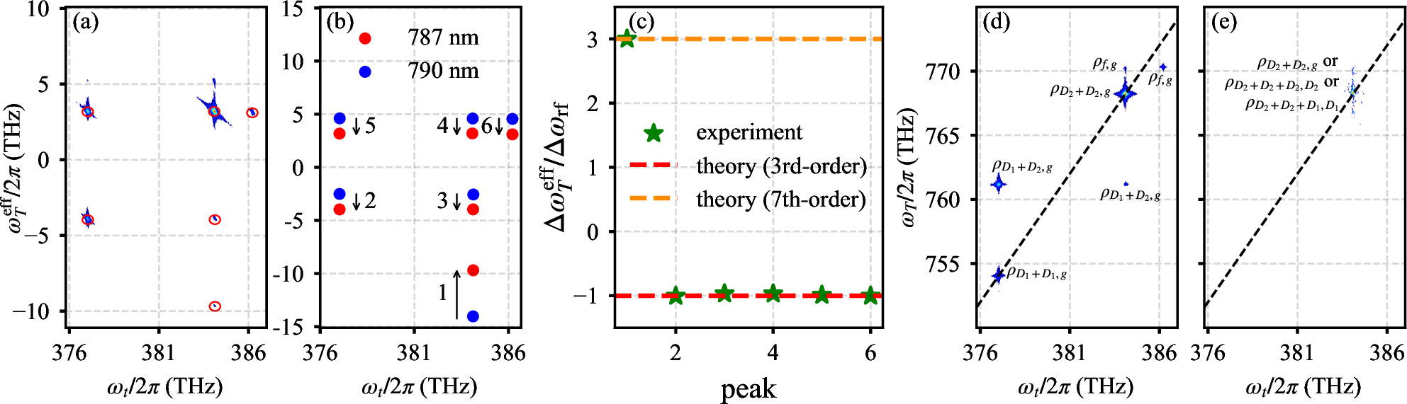
The 2Q spectrum of \(^{87}\text{Rb}\) in the panel (d) exhibit peak locations consistent with those reported in other works [18], [22], [26]. In particular, in Fig. 4 (d), the peaks at \((\omega_{t}/2\pi=384.2\text{THz},\omega_{T}/2\pi=770.5\text{THz})\) and \((\omega_{t}/2\pi=386.3\text{THz},\omega_{T}/2\pi=770.5\text{THz})\) correspond to the doubly excited state of an individual \(^{87}\text{Rb}\) atom. The other four peaks correspond to collective resonances resulting from dipole–dipole interactions in \(D_{1}+D_{1}\), \(D_{1}+D_{2}\), and \(D_{2}+D_{2}\) transitions between two \(^{87}\text{Rb}\) atoms. In Fig. 4 (e), the peak at \((384.2\text{THz},768.4\text{THz})\) arises from collective resonances generated by the dipole-dipole interaction among the multiple \(^{87}\text{Rb}\) atoms. Signals in Fig. 4 (d) are of the third order, with the phase-matching condition \(\mathbf{k}_{s}=\mathbf{k}_{2}+\mathbf{k}_{1}-\mathbf{k}_{1'}\). For the two peaks at \((\omega_{t}/2\pi=384.2\text{THz},\omega_{T}/2\pi=770.5\text{THz})\) and \((\omega_{t}/2\pi=386.3\text{THz},\omega_{T}/2\pi=770.5\text{THz})\), the field pair \(\mathbf{k}_{2}+\mathbf{k}_{1}\) first creates a coherence \(\rho_{f,g}\) during the time interval \(T\), and the subsequent action of \(-\mathbf{k}_{1'}\) generates either \(\rho_{D_{2},g}\) or \(\rho_{f,D_{2}}\) during the detection time \(t\). Here the state \(\left|f\right\rangle\) corresponds to the \(5^{2}S_{1/2}\leftrightarrow5^{2}D\) transition, prepared by the probe and the first pump pulse. The two peaks at \((\omega_{t}/2\pi=377.1\text{THz},\omega_{T}/2\pi=761.3\text{THz})\) and \((\omega_{t}/2\pi=384.2\text{THz},\omega_{T}/2\pi=761.3\text{THz})\) originate from a coherence \(\rho_{D_{1}+D_{2},g}\) prepared by \(\mathbf{k}_{2}+\mathbf{k}_{1}\) during the time interval \(T\). The final interaction with \(-\mathbf{k}_{1'}\) yields either \(\rho_{D_{1}+D_{2},D_{2}}\) (or effectively \(\rho_{D_{1},g}\) ) or \(\rho_{D_{1}+D_{2},D_{1}}\) (or effectively \(\rho_{D_{2},g}\) ), accounting for the two observed spectral positions. The remaining two peaks follow analogous pathways. And the peak in Fig. 4 (e) corresponds the 7th-order signal (see line 2 and 3 of Table ¿tbl:table195em?), which was seldomly isolated in previous studies.

The separation procedure for the \(S_{-}^{\mathrm{sep}}(\tau,\omega_{T}^{\mathrm{eff}},\omega_{t};\omega_{\mathrm{RF}})\) spectra is identical to that applied to \(S_{+}^{\mathrm{sep}}(\tau,\omega_{T}^{\mathrm{eff}},\omega_{t};\omega_{\mathrm{RF}})\) . Starting from the \(S_{-}^{\mathrm{sep}}(\tau,\omega_{T}^{\mathrm{eff}},\omega_{t};\omega_{\mathrm{RF}})\) spectrum, as shown in Fig. 5 (a), 3rd-order and 7th-order contributions are identified in the same manner by identifying different shift rates. By further applying the corresponding frequency-retrieval conditions, the separated 3rd-order 0Q coherence signal and the 7th-order 4Q coherence signal are obtained, as shown in Fig. 5 (b) and Fig. 5 (c), respectively. The observed 7th-order 0Q contribution corresponding to line 6 in Table. ¿tbl:table195em? is successfully isolated within the 0Q spectrum, as shown in Fig. 5 (b).
For other potential signal peaks arising from multi-atom interactions, such as the \(\rho_{3,1}\) coherence corresponding to line 4 in Table. ¿tbl:table195em?, no distinct spectral features were experimentally resolved. This is likely due to weak interaction strengths or minimal energy-level shifts, and these contributions are therefore presented primarily as theoretically possible pathways.
With the \(^{87}\mathrm{Rb}\) vapor system, we demonstrate the experimental isolation of the 7th-order nonlinear signal with the computation-assisted method. And the current method, tailored for multidimensional spectroscopy, uses four phase settings along with experimental acquisitions with three rotating frames, and substantially reduces experimental difficulties with complex phase cycling.
4 Conclusion↩︎
We have demonstrated an order-selective strategy for high-order nonlinear spectroscopy that combines rotating-frame acquisition with frame-shift tracking analysis of frame-dependent spectral shifts. In this framework, the rotating frame is used not only for sampling efficiency but also as a controlled modulation axis that encodes perturbative order through distinct peak-shift slopes. This enables systematic separation of overlapping nonlinear contributions after standard phase-cycling processing.
Using two-dimensional spectroscopy of rubidium vapor, we experimentally isolate a seventh-order response from coexisting third-order backgrounds, thereby establishing direct access to beyond-third-order coherence dynamics in a practical excitation regime. This approach is scalable to higher-order signals, provided that the corresponding pathways exhibit resolvable frame-dependent spectral shifts and sufficient signal-to-noise ratio.
5 Back matter↩︎
This work is supported by the Quantum Science and Technology-National Science and Technology Major Project (Grant No. 2023ZD0300700), and the National Natural Science Foundation of China (Grant Nos. U2230203, U2330401, 12088101).
We thank Dr. Mao-Rui Cai for helpful discussions.
The authors declare no conflicts of interest.
Data underlying the results presented in this paper are not publicly available at this time but may be obtained from the authors upon reasonable request.