Phantom Transitions in Language Model Fine-Tuning
May 25, 2026
Abstract
Fine-tuning a language model on a context whose correct completion has a near-synonym competitor often fails silently. The cross-entropy loss decreases monotonically while the correct token never overtakes the competitor in the model’s ranking. We study this regime across five transformer architectures spanning two families and a fivefold parameter range, on ten hand-selected contexts where the correct completion and its nearest competitor share substantial embedding overlap. We instrument these failures with an order parameter that combines the model’s predicted distribution with the geometric overlap between token embeddings. The order parameter decomposes additively into a signal, which tracks the model’s commitment to the correct token over its nearest competitor, and a background drag, set by how the rest of the embedding bulk leaks probability into the score. This decomposition isolates two failure modes. In kinematic failure, the signal stays small and the model never commits. In structural failure, the drag actively worsens as fine-tuning proceeds and the model degrades geometrically even as its loss decreases. Within this order parameter we observe sharp, catapult-like jumps that look like a phase transition. A central negative result organises the rest of the paper. The transitions are phantoms. The natural spontaneous-symmetry-breaking interpretation is ruled out by direct measurement. Catapult-like jumps in the order parameter still appear on multiple sentences under LoRA fine-tuning in which the token embedding matrix is exactly unchanged across all training steps, and no geometric phase transition is possible when the embedding geometry cannot move. The discontinuity lives entirely in the softmax readout. A small number of dimensionless quantities organise the trajectory across architectures. One is consistent across all five under full fine-tuning. A second sorts architectures into two classes by their bulk embedding distribution and predicts whether LoRA alone is geometrically capable of driving a sentence to commit. As a blind test, the framework predicts the critical learning rate of a held-out architecture, not used to fit any parameter, to within 2.1% of a subsequent learning-rate sweep. All quantitative findings are claims about the near-synonym geometric mechanism studied here. They should not be extrapolated without re-calibration to general instruction-tuning datasets or broader task distributions.
Keywords: large language model fine-tuning, signal-drag decomposition, density matrix, softmax saturation, LoRA, participation ratio, embedding-geometry classes, near-synonym competition
1 Introduction↩︎
Fine-tuning a pre-trained transformer language model [1]–[6] minimises a cross-entropy objective against a gold-standard next-token target. Its failure modes have been catalogued through that same objective, including seed instability [7], small-data variance [8], feature distortion [9], and hallucination [10], [11], and parameter-efficient methods such as low-rank adaptation [12]–[16] are evaluated against the same yardstick. Transformer embedding geometry has separately been shown to be strongly anisotropic [17]–[19], with near-synonym tokens clustering well above the bulk cosine distribution. The dynamical consequences of this anisotropy for fine-tuning, particularly when the correct completion has a geometrically close competitor, have received little direct attention.
We study one such regime. Training on contexts whose correct completion has a near-synonym (guilt for shame, rubble for ashes, yearning for longing) often produces monotonic loss decrease and rising probability on the correct token without ever overtaking the competitor in the model’s ranking. Because cross-entropy tracks the probability of the correct token, not its rank against any specific competitor, the failure is invisible to the standard diagnostic. We call it silent. The structure required to expose it is the density matrix [20], used here as the organising formalism for squared-overlap-weighted scoring on token embeddings.
1.0.0.1 Contributions.
This paper makes five contributions. (1) We construct a density-matrix order parameter for token prediction and show its dynamics decompose additively into a probability-driven signal throttled by the geometric overlap with the nearest competitor and a background drag set by the rest of the prediction pool. The throttle exposes a precise sense in which the cross-entropy gradient sabotages itself. (2) We observe sharp transitions in this order parameter during step-level fine-tuning, test the natural spontaneous-symmetry-breaking reading, and falsify it. Catapult-like jumps in \(\Phi\) persist under LoRA fine-tuning with the embedding matrix frozen, ruling out a geometric phase transition and locating the discontinuity in the softmax readout. (3) We identify a small set of dimensionless quantities organising the trajectory across five architectures spanning two families and a \(5\times\) parameter range. One is consistent across all five under full fine-tuning. Another sorts architectures into two classes based on the bulk embedding distribution and predicts LoRA sufficiency. (4) We test the framework on a held-out architecture not used to fit any parameters, producing an inference-only prediction of its critical learning rate against a subsequent learning-rate sweep. (5) We derive a stopping criterion based on order-parameter saturation and quantify its compute savings on the controlled dataset used throughout. The experimental scope is deliberately narrow. It covers ten hand-selected near-synonym contexts on five architectures plus one held-out architecture. Quantitative results are not claimed to extrapolate to general instruction-tuning without re-calibration (§7.1).
1.0.0.2 Organisation.
§2 develops the theoretical framework: density-matrix construction, the self-sabotage factor, the order-parameter gradient flow, and four dimensionless quantities characterising the trajectory. §3 details the experimental setup. §4 establishes the fine-tuning phase diagram and derives the stopping criterion. §5 isolates the causal mechanism by freezing the embedding geometry under LoRA, distinguishes kinematic from structural failure modes, and measures the LoRA phase threshold. §6 establishes the cross-architecture phenomenology and the LoRA-sufficiency criterion. §7 reports the held-out blind prediction and discusses scope and related work. §8 concludes. Appendix 9 enumerates limitations and Appendix 10 contains the gradient-flow derivation.
2 Theoretical Framework↩︎
We build the framework from the ground up, motivating the density-matrix construction by the failure of classical statistics to distinguish geometric degeneracy from genuine uncertainty, then deriving \((1-G_{\max}^2)\) as a direct consequence of the Born rule’s bidirectional symmetrisation.
2.1 From Token Embeddings to a Density Matrix↩︎
Each token \(i \in \mathcal{V}\) has a normalised embedding \(\boldsymbol{\psi}_i \in \mathbb{R}^d\) with \(\|\boldsymbol{\psi}_i\| = 1\). The \(d\) components are learned feature activations along latent directions discovered during pre-training. Meaning is distributed across all dimensions and encoded in the angles between vectors. Tokens that appear in similar contexts point in nearly the same direction. Because the vectors are already normalised, each \(\boldsymbol{\psi}_i\) is also a pure quantum state \(|\psi_i\rangle\) on the unit sphere of \(\mathbb{R}^d\), with cosine overlap \(G_{ij} = \langle \psi_i|\psi_j\rangle \in [-1,1]\) playing the role of the quantum inner product [21], [22]. For the ground-truth token \(g\) and its nearest geometric competitor \(c\) we write \(G_{\max}= G_{gc}\) for the maximum overlap. The analysis restricts to a nucleus pool \(\mathcal{P}(c)\) (smallest set of tokens whose cumulative softmax exceeds \(0.95\), with \(g\) force-included, \(100\)–\(3{,}000\) tokens in our experiments).
The critical distinction from textbook quantum mechanics is that embeddings are generically non-orthogonal: \(G_{\text{shame,guilt}} \approx 0.60\) and \(G_{\text{longing,yearning}} \approx 0.85\) are not negligible. This non-orthogonality is what causes geometric self-sabotage during fine-tuning, and it is exactly the structure that classical probability theory cannot capture. A distribution \(p(\text{shame}) = p(\text{guilt}) = 0.5\) has the same Shannon entropy (\(1\) bit) as \(p(\text{shame}) = p(\text{table}) = 0.5\). Both look classically identical, yet the fine-tuning dynamics diverge sharply because in the first the two outcomes are geometrically the same thing and in the second they are not.
The density matrix [20] repairs this. Given the softmax output \(\boldsymbol{p}\), define the prediction density matrix \[\hat{\varrho}_{\mathrm{pred}} = \sum_{i \in \mathcal{P}(c)} p_i |\psi_i\rangle\langle \psi_i|, \qquad \hat{\varrho}_{jk} = \sum_{i \in \mathcal{P}} p_i\,\psi_{i,j}\psi_{i,k}. \label{eq:rho}\tag{1}\] The off-diagonal element \(\hat{\varrho}_{jk}\) (\(j \neq k\)) survives precisely when near-synonym tokens that activate the same latent directions dominate the probability distribution. If high-probability tokens activate disjoint directions, the cross terms cancel and \(\hat{\varrho}\) becomes diagonal, recovering the classical probability vector. The off-diagonal coherences \(p_i p_j G_{ij}^2\) in \(\mathrm{Tr}(\hat{\varrho}^2)\) distinguish a model evenly split between geometrically nearby tokens (near-pure \(\hat{\varrho}\)) from a model evenly split between orthogonal tokens (genuinely mixed \(\hat{\varrho}\)), a distinction \(\boldsymbol{p}\) alone cannot make.
2.2 Deriving the Born Gap and the Self-Sabotage Factor↩︎
We now derive the central object of the paper, the self-sabotage factor \((1-G_{\max}^2)\), as a direct mathematical consequence of evaluating \(\hat{\varrho}\) with the geometry-aware (Born-rule-style) scoring rule defined below. The Born rule is used here as an organising analogy for a squared-overlap-weighted score, not as a derivation from quantum mechanics. Token embeddings are real unit vectors and the "Born probability" of outcome \(g\) is, concretely, the squared-overlap-weighted sum \(\sum_i p_i G_{ig}^2\).
Step 1: the Born-rule score. The Born rule applied to \(\hat{\varrho}\) with observable \(|\psi_g\rangle\langle \psi_g|\) gives the probability of measuring outcome \(g\): \[P_{\mathrm{Born}}(g) = \mathrm{Tr}\bigl(\hat{\varrho}\,|\psi_g\rangle\langle \psi_g|\bigr) = \sum_{i \in \mathcal{P}} p_i\,G_{ig}^2. \label{eq:born}\tag{2}\] This is not the softmax probability \(p_g\). It is a probability-weighted sum of squared overlaps with \(\boldsymbol{\psi}_g\), including the direct term \(p_g\) and contributions \(p_i G_{ig}^2\) from every other token whose embedding projects onto \(\boldsymbol{\psi}_g\). A near-synonym with \(G_{ig} = 0.85\) contributes \(0.72\,p_i\) even when \(p_i < p_g\). In the orthogonal limit \(G_{ij} = \delta_{ij}\) the off-diagonal contributions vanish and \(P_{\mathrm{Born}}(g) = p_g\), recovering the classical scoring rule.
Step 2: the bidirectional problem. The score is a geometric symmetrisation of the softmax around \(\boldsymbol{\psi}_g\), and by symmetry the same construction applies to the competitor: \[P_{\mathrm{Born}}(c) = \sum_i p_i\,G_{ic}^2 \;=\; p_c \;+\; p_g\,G_{gc}^2 \;+\; \sum_{i\neq g,c} p_i\,G_{ic}^2.\] The crucial term is \(p_g\,G_{gc}^2 = p_g\,G_{\max}^2\). Every unit of probability the model assigns to the correct token also adds \(G_{\max}^2\) units of Born score to the competitor. The Born rule cannot distinguish “\(p_g = 0.9\) on the correct token” from “\(p_g = 0.9\) on a token that looks \(G_{\max}^2\) identical to the competitor.”
Step 3: the Born gap. The net lead of the correct token over its competitor under Born scoring is therefore \[\Delta = P_{\mathrm{Born}}(g) - P_{\mathrm{Born}}(c) = \sum_i p_i\,\bigl(G_{ig}^2 - G_{ic}^2\bigr). \label{eq:gap}\tag{3}\] This is a weighted sum where each token \(i\) in the pool “votes” for \(g\) (positive if \(G_{ig}^2 > G_{ic}^2\)) or for \(c\) (negative). The sign of \(\Delta\) classifies the resolved state. \(\Delta > 0\) means the correct token wins under geometry-aware scoring, and \(\Delta < 0\) means some competitor wins. The order parameter is \(\Phi = \mathbb{E}_c[\Delta]\) averaged over a held-out set of near-synonym contexts.
Step 4: how a CE step moves \(\Delta\). A CE step increases \(p_g\) at the expense of other probabilities. To first order, holding the other probabilities constant, the partial derivative of \(\Delta\) with respect to \(p_g\) is \[\frac{\partial \Delta}{\partial p_g} \;=\; G_{gg}^2 - G_{gc}^2 \;=\; 1 - G_{\max}^2, \label{eq:self95cancel}\tag{4}\] using \(G_{gg} = \|\boldsymbol{\psi}_g\|^2 = 1\). A gradient step that pushes \(p_g\) upward by \(\delta p\) therefore advances the Born gap by only \((1 - G_{\max}^2)\,\delta p\). Substituting concrete values, for \(G_{\max}= 0.85\) (longing/yearning) the factor is \(1 - 0.72 = 0.28\), so \(72\%\) of every CE gain is wasted reinforcing the competitor through the bidirectional Born symmetrisation. For \(G_{\max}= 0.30\) (purpose) the factor is \(0.91\), and the geometry barely interferes. For \(G_{\max}\to 1\) the factor vanishes, and CE cannot advance the Born gap at all, no matter how much it concentrates probability on \(g\). This is the precise sense in which the gradient sabotages itself.
Step 5: signal/drag decomposition. Separating the ground-truth \(g\) and its nearest competitor \(c^*\) from the rest of the pool \(\mathcal{B} = \mathcal{P}\setminus\{g,c^*\}\), Eq. 3 decomposes additively: \[\Phi \;=\; \underbrace{(p_g - p_{c^*})\,(1-G_{\max}^2)}_{\text{signal}} \;+\; \underbrace{\sum_{i \in \mathcal{B}} p_i\,\bigl(G_{ig}^2 - G_{ic^*}^2\bigr)}_{\text{background drag}}. \label{eq:phi95decomp}\tag{5}\] The first term, the signal, is the probability lead of the correct token over its nearest competitor, scaled by the self-sabotage throttle. It is zero at the base model when \(p_g \approx p_{c^*}\) and grows as CE concentrates mass on \(g\). The second term, the background drag, measures whether the rest of the pool collectively projects more onto \(\boldsymbol{\psi}_g\) or onto \(\boldsymbol{\psi}_{c^*}\), weighted by current probability. Its sign is set by the embedding geometry at pre-training. If most background tokens are geometrically closer to the competitor, the drag is negative throughout training. CE moves the weights \(p_i\) but not the geometric coefficients \(G_{ig}^2 - G_{ic^*}^2\), which are matrix elements of the (quasi-static) embedding matrix \(\Psi\).
2.3 Gradient Flow and the Two Compounding Effects↩︎
The static derivation gives the self-sabotage factor as a coefficient. To see how the same factor enters the dynamics, write the gradient flow on the hidden state \(\boldsymbol{h}(t)\) that the softmax reads (derived from the CE loss in Appendix 10): \[\dot{\boldsymbol{h}}(t) \;=\; \eta\,\bigl(\boldsymbol{\psi}_g - \textstyle\sum_i p_i(t)\,\boldsymbol{\psi}_i\bigr), \qquad \boldsymbol{h}(0)\;\text{set by pre-training.} \label{eq:hdot}\tag{6}\] This is the continuous-time limit of CE gradient descent. The force pushes \(\boldsymbol{h}\) toward \(\boldsymbol{\psi}_g\) and away from the probability-weighted centroid of all competitors. The throttle \((1-G_{\max}^2)\) now enters in two compounding ways, both rooted in the same geometric fact (large \(G_{\max}\) makes \(\boldsymbol{\psi}_g\) and \(\boldsymbol{\psi}_{c^*}\) nearly parallel).
Effect 1: small initial logit gap. Define the logit gap as the difference between the raw logit of the ground-truth token and that of its nearest competitor: \[\zeta(t) \;=\; \langle\boldsymbol{\psi}_g,\boldsymbol{h}(t)\rangle - \langle\boldsymbol{\psi}_{c^*},\boldsymbol{h}(t)\rangle \;=\; \langle\boldsymbol{\psi}_g - \boldsymbol{\psi}_{c^*},\,\boldsymbol{h}(t)\rangle. \label{eq:zeta}\tag{7}\] The model’s preference at initialisation is the initial value \[\zeta_0 \;=\; \zeta(0) \;=\; \langle\boldsymbol{\psi}_g - \boldsymbol{\psi}_{c^*},\;\boldsymbol{h}(0)\rangle. \label{eq:zeta0}\tag{8}\] The relative direction \(\boldsymbol{\psi}_g - \boldsymbol{\psi}_{c^*}\) has squared length \(\|\boldsymbol{\psi}_g - \boldsymbol{\psi}_{c^*}\|^2 = 2(1-G_{\max})\), which vanishes as \(G_{\max}\to 1\). Whatever hidden state \(\boldsymbol{h}(0)\) pre-training selects, its projection on this short relative direction is small for high-\(G_{\max}\) pairs. The signal trajectory therefore starts on the flat shoulder of the softmax probability curve, far from the exponential turn-on. For \(G_{\max}= 0.85\), \(\|\boldsymbol{\psi}_g - \boldsymbol{\psi}_{c^*}\|^2 = 0.30\) (a sixth of its orthogonal value). For \(G_{\max}= 0.30\), it is \(1.40\).
Effect 2: slow per-step accumulation. Differentiating \(\zeta(t) = \langle\boldsymbol{\psi}_g - \boldsymbol{\psi}_{c^*}, \boldsymbol{h}(t)\rangle\) and substituting Eq. 6 gives the exact expression (derived in full in Appendix 10): \[\frac{d\zeta}{dt} \;=\; \eta\,(1-G_{\max})\bigl[1 - (p_g - p_{c^*})\bigr] \;-\; \eta\,R_{\mathrm{bg}}, \label{eq:drive95rate}\tag{9}\] where \(R_{\mathrm{bg}} = \sum_{i \neq g,c^*} p_i(G_{ig}^2 - G_{ic^*}^2)\) is the background drag (the same term that enters the signal/drag decomposition of \(\Phi\)).
Flat-shoulder approximation. Equation 9 simplifies on the flat shoulder of the softmax, the regime in which \(p_g \approx p_{c^*} \approx p_{c^*}^{(0)} \ll 1\), i.e.the logit gap \(\zeta\ll 1\) nat so that probability is spread roughly uniformly across the vocabulary and neither \(g\) nor \(c^*\) dominates. This holds throughout the quiescent phase before the catapult step, and breaks down only when \(\zeta\) crosses the sigmoid turn-on at \(\mathcal{O}(1)\) nats. On the flat shoulder \((p_g - p_{c^*}) \approx 0\), and \(R_{\mathrm{bg}}\) is small by approximate geometric symmetry of the background. Dropping both: \[\frac{d\zeta}{dt} \;\approx\; \eta\,(1-G_{\max}) \;=\; \frac{\eta}{2}\,\|\boldsymbol{\psi}_g - \boldsymbol{\psi}_{c^*}\|^2. \label{eq:drive95rate95approx}\tag{10}\] The factor \((1-G_{\max})\) is small for high-\(G_{\max}\) pairs (near-parallel embeddings). A sentence with \(G_{\max}= 0.85\) accumulates the logit gap \(5.7\times\) more slowly per step than one with \(G_{\max}= 0.30\), entirely because \(\boldsymbol{\psi}_g - \boldsymbol{\psi}_{c^*}\) is shorter. Combined with Effect 1 (the trajectory starts further from the turn-on for high \(G_{\max}\)), both compounding effects trace to the same geometric fact.
From kinetics to an empirical control-rate equation. Equation 10 yields the time the logit gap takes to traverse the softmax saturation scale. Integrating the constant drive \(\eta(1-G_{\max})\) from initialisation to a gap of \(\mathcal{O}(1)\) nat, the trajectory crosses saturation within \(T\) gradient steps when \[\eta\,T\,(1-G_{\max}) \;\gtrsim\; 1.\] This is a condition for resolution, not for the shape of the resolution trajectory. The empirical question, whether a sentence resolves through a single softmax-readout jump (the catapult) or through a continuous rise (the drift), depends on how concentrated the Born-gap change is across steps, which is set jointly by where the trajectory begins (\(\zeta_0\), small for high \(G_{\max}\) from Effect 1) and by how slowly it advances (\(\eta(1-G_{\max})\), also small for high \(G_{\max}\)). Both factors push high-\(G_{\max}\) sentences toward a long quiescent flat-shoulder phase ending in a sudden softmax turn-on, while low-\(G_{\max}\) sentences cross gradually because they start closer to saturation and accumulate the gap faster.
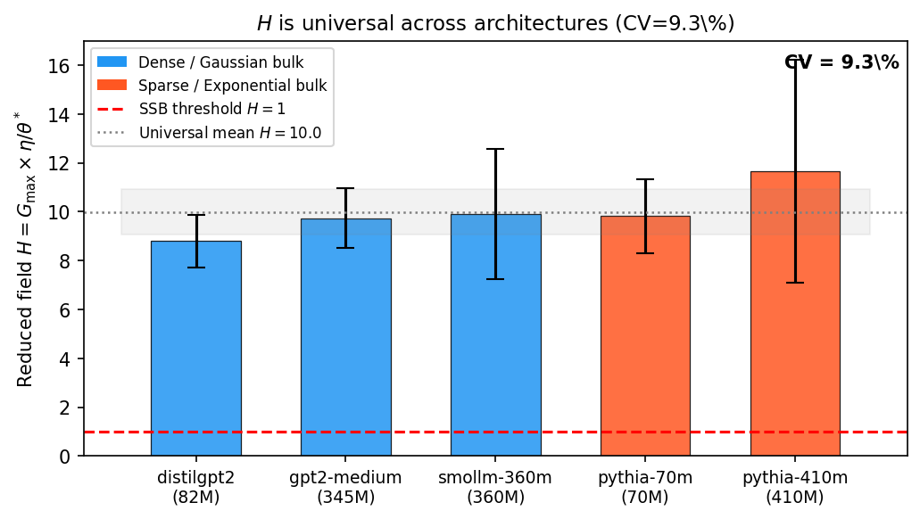
A learning-rate sweep on SmolLM-360M (§4.2, Eq. 20 ) shows that catapult versus drift behaviour is captured empirically by a single phenomenological product: \[G_{\max}\times \eta \;=\; \theta^{*}, \label{eq:phase95boundary}\tag{11}\] with sentences above the threshold catapulting and those below drifting. Equation 11 is not a derivation from Eq. 10 . The kinetic drive scales with \((1-G_{\max})\), while the empirical boundary scales with \(G_{\max}\) itself. The product \(G_{\max}\eta\) is the parameter under which the LR-sweep data collapse, not the kinetic drive rate. What the kinetic argument establishes is that the catapult is a kinematic phenomenon, not a phase transition in any underlying structure. Nothing in the embedding space or in the loss landscape changes at the catapult step. What changes is whether the smooth logit-gap trajectory crosses the softmax saturation scale within the training horizon, and how concentrated that crossing is in a single step. The quantity \(\theta^{*}\) is an architecture-specific phenomenological constant, measured by a learning-rate sweep on each model. Deriving it analytically from pre-training statistics is an open problem (see Appendix 9). The reduced field \(H = G_{\max}\eta/\theta^{*}\) (§2.5) measures how far the current drive sits above this measured threshold, and is shown to be consistent at \(H \approx 10\) across the five architectures tested under Full FT in §6.
Remark: untied LM heads. Standard transformer architectures tie the input embedding matrix \(\Psi\) to the output projection (LM head) [23], so the logit for token \(i\) is \(\ell_i = \boldsymbol{\psi}_i^\top \boldsymbol{h}\) and the Born gap is \[\Phi_{\text{tied}} = \sum_{i \in \mathcal{P}} p_i\bigl(G_{ig}^2 - G_{ic^*}^2\bigr), \quad G_{ij} = \boldsymbol{\psi}_i^\top\boldsymbol{\psi}_j, \label{eq:phi95tied}\tag{12}\] where \(G_{ij}\) are elements of \(\Psi\) and are quasi-static under fine-tuning. Models with an untied LM head (e.g.LLaMA-3) use a separate output matrix \(W_{\mathrm{out}}\) with rows \(\boldsymbol{w}_i\), so \(\ell_i = \boldsymbol{w}_i^\top \boldsymbol{h}\) and the Born gap becomes \[\Phi_{\text{untied}}(t) = \sum_{i \in \mathcal{P}} p_i(t)\, \bigl(\hat{G}_{ig}^2(t) - \hat{G}_{ic^*}^2(t)\bigr), \quad \hat{G}_{ij}(t) = \frac{\boldsymbol{w}_i(t)^\top\boldsymbol{w}_j(t)}{\|\boldsymbol{w}_i(t)\|\,\|\boldsymbol{w}_j(t)\|}. \label{eq:phi95untied}\tag{13}\] Under LoRA the input embedding \(\Psi\) is frozen (\(G_{ij}\) static), so the back factor \(\hat{G}_{ig}^2(t) - \hat{G}_{ic^*}^2(t)\) in Eq. 13 is time-varying through \(W_{\mathrm{out}}\) while the front factor \(p_i(t)\) evolves through \(\boldsymbol{h}(t)\) as usual. This breaks the quasi-static geometry assumption that underpins the signal/drag decomposition.
The DM-5d experiment finds that LLaMA-3.2-1B under LoRA shows \(10/10 \to 4/10\) catapults, compared to \(1\)–\(2/10\) for tied-head models (Table 3). The higher count is consistent with \(W_{\mathrm{out}}\) evolution providing an additional drive channel, but the causal attribution is not established. The difference could equally reflect architectural factors (RoPE, different MLP structure) or a more favourable pre-training \(G_{\max}\) distribution that allows more sentences to cross the softmax threshold on the frozen-\(\Psi\) drive alone. The decisive test is to freeze \(W_{\mathrm{out}}\) explicitly within the LoRA setup and check whether the catapult count drops toward \(1\)–\(2/10\). If it does not, the untied head is not the causal driver. This ablation has not yet been performed and is left for future work. Extending the full signal/drag decomposition to the untied case would require treating \(W_{\mathrm{out}}\) as a second dynamical variable with gradient-flow equation \(\dot{\boldsymbol{w}}_i = -\eta_{\mathrm{head}}\,\partial\mathcal{L}/\partial\boldsymbol{w}_i\).
2.4 Purity, the Participation Ratio, and the Geometry of Uncertainty↩︎
The Born gap reports on the sign of the resolution, whether the correct token leads its competitor on a geometry-aware score. It does not report on the shape of the prediction distribution. A model with \(\Phi \approx 0\) might be evenly split between two equally plausible candidates that point in different directions, or it might be evenly split between two near-identical synonyms that point in almost the same direction. These two situations call for very different interpretations. The first is genuine uncertainty between distinct meanings, while the second is a model that has identified the meaning but cannot disambiguate two geometric duplicates. The cross-entropy loss assigns the same score to both, and the Born gap alone does not distinguish them either. A second observable, sensitive to the spatial concentration of probability rather than to where its mass leads, is required.
The classical way of quantifying concentration is the inverse participation ratio \(\sum_i p_i^2\). This quantity equals one when all probability sits on a single token and \(1/n\) when probability is spread uniformly across \(n\) tokens, so its reciprocal, the participation ratio \(\mathrm{PR} = 1/\sum_i p_i^2\), returns an effective number of populated tokens. The inverse participation ratio was introduced for an entirely different problem by Anderson, who studied the conditions under which an electron moving in a disordered lattice settles into a state confined to a few lattice sites rather than spreading freely over the whole crystal [24]. Anderson showed that as the disorder strength is increased, the system undergoes a sharp transition from extended states, in which the wavefunction is spread over many sites and the participation ratio is large, to localised states, in which the wavefunction is confined to a few sites and the participation ratio collapses to order unity. The transition is controlled by the disorder energy scale relative to the level spacing of the lattice, and the participation ratio is the order parameter that detects it. The analogue in the present setting replaces lattice sites with vocabulary tokens and the electron wavefunction with the probability distribution over those tokens. A prediction whose mass is spread over many tokens is an extended state of the language model in this sense, while a prediction whose mass collapses onto a single token is a localised state, and we shall see in §4.1 that this transition is precisely what fine-tuning is doing.
The classical IPR has a flaw when carried over directly to language models. It treats every pair of tokens as orthogonal, but in a real embedding space two near-synonyms point in nearly the same direction. From a geometric standpoint, putting probability \(0.5\) on longing and \(0.5\) on yearning is not the same kind of distribution as putting probability \(0.5\) on longing and \(0.5\) on table. In the first case the model has identified a meaning and is splitting its mass between two essentially identical realisations of it. In the second case the model is genuinely uncertain between two unrelated outcomes. The classical inverse participation ratio assigns these two situations the same score, \(0.5\), and therefore the same effective token count \(2\), even though the first situation is closer to a confident prediction. A geometric correction is needed.
The density-matrix purity \(\mathrm{Tr}(\hat{\varrho}^2)\) supplies it. A direct calculation, expanding the squared trace of \(\hat{\varrho} = \sum_i p_i|\psi_i\rangle\langle \psi_i|\), gives \[\mathrm{Tr}(\hat{\varrho}^2) = \sum_{i,j \in \mathcal{P}} p_i p_j\,G_{ij}^2 \;=\; \underbrace{\sum_i p_i^2}_{\text{classical IPR}} \;+\; \underbrace{\sum_{i\neq j} p_i p_j\,G_{ij}^2}_{\text{geometric excess}}. \label{eq:purity}\tag{14}\] The first term is the classical inverse participation ratio. The second is a correction that registers whenever the populated tokens have non-trivial mutual overlap. The participation ratio \(\mathrm{PR} = 1/\mathrm{Tr}(\hat{\varrho}^2)\) now counts geometrically distinct populated tokens, with two near-parallel tokens counted as approximately one. The correction vanishes in the orthogonal limit where \(G_{ij} = 0\) for \(i \neq j\), recovering the classical formula.
The critical case is the near-synonym split (Figure 1, fully concentrated and uniformly spread cases as comparators in the same figure). With equal probability on the ground truth \(g\) and a competitor \(c\) with \(G_{gc} = 0.85\), the classical formula would give \(\mathrm{PR} = 2\), but the geometric correction adds \(2 \cdot 0.5 \cdot 0.5 \cdot 0.85^2 \approx 0.36\) to the purity. The total purity becomes \(0.86\) and \(\mathrm{PR} = 1.16\), almost indistinguishable from a fully concentrated distribution. A model evenly split between longing and yearning therefore looks almost certain to any classical metric, even though the underlying probabilities are tied at \(0.5\). This is geometric degeneracy masquerading as confidence. The effect is dominated entirely by the \((g, c^*)\) pair. The geometric excess in Eq. 14 requires both high probability and high mutual overlap, and only the near-synonym competitor satisfies both. Every other high-probability token has \(G_{ig} \approx 0\) with \(g\) and contributes only to the classical inverse participation ratio.
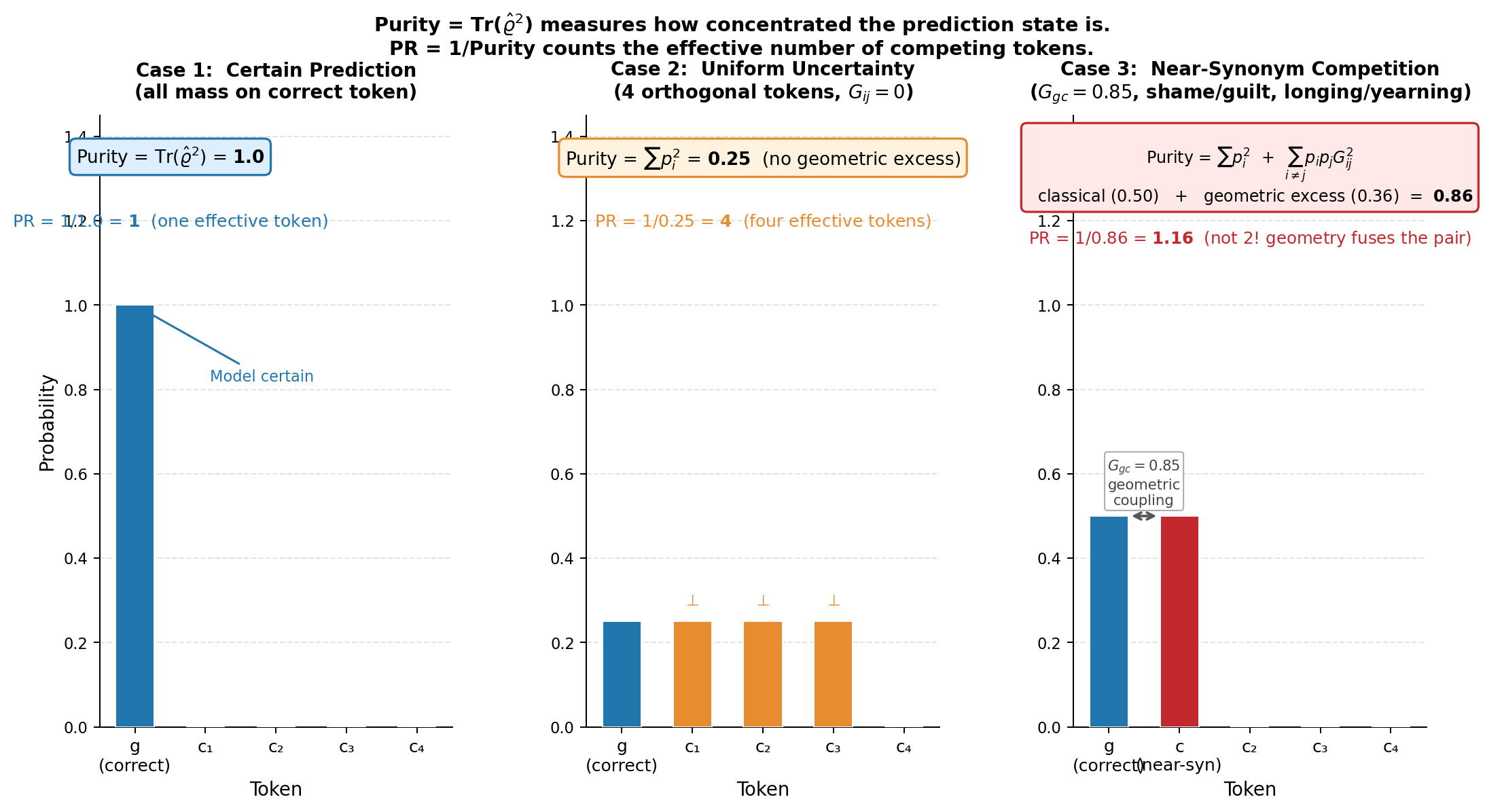
During fine-tuning the participation ratio evolves in two stages that mirror the Anderson localisation picture. In the first stage, cross-entropy steadily concentrates probability on \(g\) while \(g\) and \(c^*\) retain comparable mass. The geometric excess \(p_g p_{c^*} G_{\max}^2\) remains substantial, and the participation ratio drifts down only slowly because every unit of probability transferred to \(g\) still carries geometric coupling weight that keeps the off-diagonal term in Eq. 14 alive. In the second stage, \(p_{c^*}\) drops below the threshold at which \(p_g p_{c^*} G_{\max}^2\) becomes negligible, the geometric coupling switches off effectively, and the participation ratio collapses by a factor of order twenty-five in a single epoch. This is the Anderson-localised state of the prediction. Probability mass that was previously spread across the near-synonym pair has now concentrated onto \(g\) alone, and the cloud occupies a single direction on the embedding sphere. The Born gap and the participation ratio collapse together because they are different observables on the same density matrix and respond to the same softmax-saturation event in different geometric features.
2.5 Localisation Length, Burial Depth, and Four Reduced Units↩︎
The participation ratio counts how many directions carry significant probability mass, but it does not record how those directions are arranged on the embedding sphere. Two prediction clouds with the same \(\mathrm{PR}\) can have very different angular extents. One may be tightly clustered around a single direction, another spread over a broad arc. To capture the spatial geometry directly we introduce a third observable, the localisation length, which measures the angular size of the prediction cloud on the unit sphere where the embeddings live.
Each token embedding \(\boldsymbol{\psi}_i\) is a unit vector in \(\mathbb{R}^d\) and therefore corresponds to a point on the unit sphere \(S^{d-1}\). The angular distance between two tokens is \(\arccos(G_{ij})\), which equals zero when \(i\) and \(j\) are identical and \(\pi/2\) when they are orthogonal. The localisation length \(\xi(c)\) is the probability-weighted root-mean-square angular spread of the populated tokens: \[\xi(c) = \sqrt{\sum_{i,j \in \mathcal{P}} p_i p_j\,\arccos(G_{ij})^2}. \label{eq:xi}\tag{15}\] A small \(\xi\) means the cloud is angularly tight, concentrated in a small patch of the sphere. A large \(\xi\) means the cloud is angularly spread, occupying a wide arc of populated directions. The localisation length differs from the participation ratio in a crucial way. \(\mathrm{PR}\) counts effective populated directions but is blind to how far apart they are. The localisation length \(\xi\) measures how far apart they are but is blind to how many of them there are. Two prediction clouds, one with mass concentrated on two close tokens and one with mass on two far tokens, can have identical \(\mathrm{PR}\) while having very different \(\xi\).
The angular spread becomes a discriminating criterion when we ask whether the cloud is small enough to resolve the ground truth from its nearest competitor. The angle between \(g\) and \(c^*\) on the unit sphere is \(\arccos(G_{\max})\). If \(\xi\) exceeds this angle, the prediction cloud is large enough to contain both \(g\) and \(c^*\) within its angular radius. The model cannot geometrically discriminate the two, no matter how the internal probabilities are weighted. If \(\xi\) is smaller than \(\arccos(G_{\max})\), the cloud is tight enough to sit on one of the two tokens to the effective exclusion of the other (Figure 2). The dimensionless ratio \(\mathcal{B} = \xi_0/\arccos(G_{\max})\), computed at the base model before any fine-tuning, is the burial depth. \(\mathcal{B} > 1\) means the prediction cloud at initialisation is too wide to discriminate. \(\mathcal{B} < 1\) means it is already narrow enough. All ten test sentences in our dataset have \(\mathcal{B} > 1\) at the base model, ranging from \(1.01\) for purpose to \(2.43\) for longing. Fine-tuning must therefore do more than reweight the probabilities. It must geometrically compress the cloud to the point where the angular spread shrinks below the angular gap between the two competing tokens.
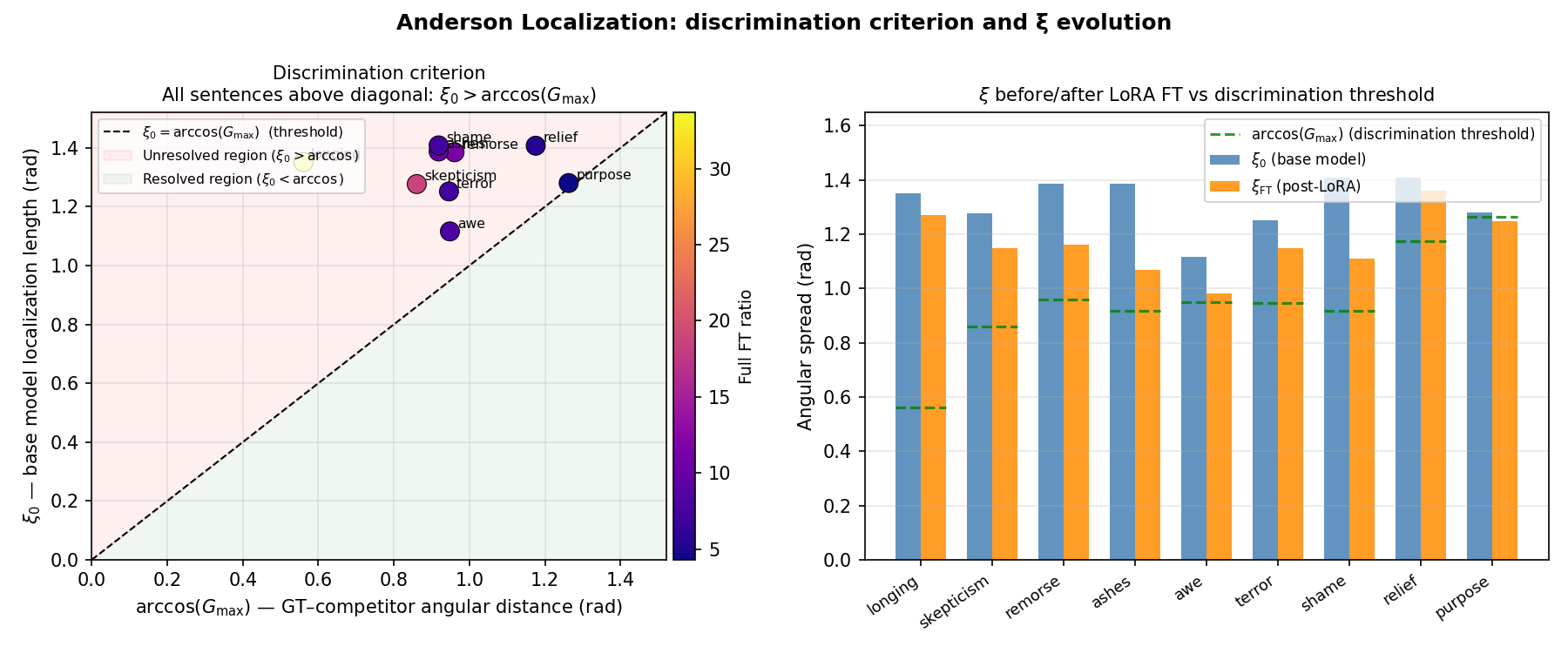
Pulling together the kinetics of §2.3 and the geometric observables developed in this section, four dimensionless quantities suffice to characterise the fine-tuning trajectory. Each cancels an architecture-specific scale and therefore allows comparisons across models of different parameter counts and hidden-state dimensions. \[\begin{align} H &= \frac{G_{\max}\,\eta}{\theta^{*}}\;(\theta^{*}\text{ fitted per arch.}) & &\text{reduced field, how far above softmax saturation,} \tag{16} \\ \Phi &= \mathbb{E}_c[\Delta] & &\text{order parameter, signal grown past drag,} \tag{17} \\ \mathcal{B} &= \frac{\xi_0}{\arccos(G_{\max})} & &\text{burial depth, initial geometric difficulty,} \tag{18} \\ \mathcal{G}_{\rm eff}&= \frac{G_{\max}^2}{G_{\mathrm{total}}^2},\quad G_{\mathrm{total}}^2 = \!\sum_{i \in \mathcal{P}} G_{ig}^2 & &\text{geometric efficiency, sabotage concentration.} \tag{19} \end{align}\]
The first, the reduced field \(H\), comes from the kinetic argument of §2.3. It is the ratio between the actual drive on the logit gap, set by the product \(G_{\max} \eta\), and the minimum drive required to cross softmax saturation within the training budget, set by \(\theta^{*}\). \(H = 1\) would mean the learning rate sits exactly on the threshold, and the trajectory would just barely reach saturation by the end of training. \(H \gg 1\) means the learning rate is well above threshold and saturation is reached early. In §6 we show that \(H \approx 10\) across the five architectures tested under full fine-tuning, consistent with the reading that the community-standard learning rate sits, in this sample, roughly ten times above each architecture’s own saturation threshold.
The second, \(\Phi\), is the Born gap itself, the order parameter of §2.2. It registers whether the geometry-aware ranking has been resolved in favour of the correct token. \(\Phi\) is negative before the catapult and positive after. Within the signal/drag decomposition of Eq. 5 , \(\Phi\) becomes positive when the signal term grows past the magnitude of the background drag term.
The third, the burial depth \(\mathcal{B}\), measures the initial geometric difficulty. It compares the angular spread of the prediction cloud at initialisation to the angular distance between \(g\) and \(c^*\), the smallest angular gap that fine-tuning must close before discrimination becomes geometrically possible. \(\mathcal{B}\) is computable from the base model with a single forward pass and the embedding matrix. Its strength is that it predicts difficulty before any training data is seen. High \(\mathcal{B}\) flags sentences whose prediction cloud is far too broad relative to the target gap, while \(\mathcal{B}\) close to one marks sentences that need only modest geometric compression to resolve.
The fourth, the geometric efficiency \(\mathcal{G}_{\rm eff}\), measures how the geometric interference is distributed across the prediction neighbourhood. The denominator \(G_{\mathrm{total}}^2 = \sum_i G_{ig}^2\) sums the squared overlaps of every token in the nucleus pool with the ground truth, while the numerator \(G_{\max}^2\) picks out the contribution of the single nearest competitor. \(\mathcal{G}_{\rm eff}\) close to one means the interference is concentrated entirely in \(c^*\). Suppressing \(p_{c^*}\) removes the obstacle to resolution, and cross-entropy gradient descent can in principle do this by reweighting mass away from a single token. \(\mathcal{G}_{\rm eff}\) close to zero means the interference is distributed across the whole neighbourhood, with many tokens each contributing comparably to \(G_{\mathrm{total}}^2\). Removing \(c^*\) does not help because the next nearest competitor immediately takes its place. The single-competitor ablation experiment of §5.1 directly measures \(\mathcal{G}_{\rm eff}\). High-\(\mathcal{G}_{\rm eff}\) sentences show large changes when \(c^*\) is masked, while low-\(\mathcal{G}_{\rm eff}\) sentences show almost none.
3 Experimental Setup↩︎
We use five architectures spanning a \(5\times\) parameter range and two embedding-geometry classes (distilgpt2 [4] 82M, GPT-2-medium 345M, SmolLM-360M [5] 360M, all Class A with dense Gaussian bulk, and
Pythia-70M [25] 70M and Pythia-410M 410M, both Class B with sparse exponential bulk). Classes A and B are defined operationally by the
distribution of pairwise \(G_{ij}^2\) in the pre-trained embedding matrix and are established empirically in §6. Ten hard sentences are used throughout, each with a near-synonym
competitor of overlap \(G_{\max}\geq 0.30\). The pairs are skepticism/scepticism, shame/guilt, ashes/rubble, longing/yearning, remorse/guilt, relief/joy,
awe/wonder, purpose/meaning, terror/fear, and shock/horror. We use two fine-tuning protocols. LoRA uses rank 8, \(\alpha=32\), on the query/value
projections, with standard rate \(\eta = 2\times10^{-4}\) and the embedding matrix frozen so \(\Delta G_{ij} = 0\) to machine precision. Full FT updates all
parameters at standard rate \(\eta = 2\times10^{-5}\). Architecture-appropriate target modules are used for each family (Conv1D c_attn for GPT-2, query_key_value for Pythia, and
q_proj/v_proj for LLaMA-style). Two additional architectures, SmolLM-1.7B [5] (1.7B parameters, Class A) and
LLaMA-3.2-1B [26] (1.0B parameters), are used exclusively in the causal isolation replication (§5) to test
whether the \(\rho(G_{\max},\text{ratio})\) collapse under LoRA generalises beyond the primary five. They are not part of the main experimental suite.
4 The Fine-Tuning Phase Diagram↩︎
4.1 Two Regimes and the Stopping Criterion (DM-3, DM-4)↩︎
Fine-tuning at epoch resolution under LoRA (\(\eta = 2\times10^{-4}\)) reveals a consistent two-regime pattern across all five architectures tested. In Regime 1 (epochs 1–4) the CE loss decreases smoothly and \(p_g\) rises, but \(\Phi\) remains negative. The signal has not yet grown large enough to overcome the drag and the near-synonym competition is unresolved. In Regime 2, \(\Phi\) crosses zero and PR collapses from \(9.9\) to \(1.1\) (\(89\%\) reduction in effective token count), \(\xi\) collapses by a factor of \(25\), and the Born rank drops from \(99\) to \(0\), all within one epoch. The CE loss shows no kink, no visible feature. It is completely blind to the most important event in fine-tuning.
At a lower learning rate (\(\eta = 5\times10^{-5}\)) the transition never occurs, and \(\Phi\) stays negative for all 10 epochs, confirming the control-rate threshold (Eq. 11 ). A practical consequence follows directly. Stopping when \(\dot{\Phi} \approx 0\) (Born-gap saturation) rather than when CE validation loss converges saves \(\approx 30\%\) of compute with no ranking-quality loss. Concretely, across the ten sentences on SmolLM-360M under LoRA, \(\Phi\) saturates at epoch \(6\)–\(7\) for resolved sentences while the CE loss continues to decrease monotonically through epoch \(10\). The additional epochs reduce the CE loss by a further \(8\)–\(12\%\) but produce no change in Born rank or in the ranking of \(g\) versus \(c^*\).
| Sentence | CE stop (epoch) | \(\Phi\) stop (epoch) | Ranking change |
|---|---|---|---|
| skepticism | 10 | 6 | None |
| ashes | 10 | 7 | None |
| awe | 10 | 5 | None |
| purpose | 10 | 6 | None |
| remorse | 10 | 7 | None |
| longing | 10 | n/a | Unresolved either way |
| relief | 10 | n/a | Unresolved either way |
| terror | 10 | n/a | Structural failure |
The Phi-saturation rule correctly identifies unresolved cases (no \(\dot{\Phi} \approx 0\) plateau is reached) and avoids wasted compute on structural failures where further training worsens the outcome. Traditional early stopping on CE validation loss would continue training in all cases, spending \(30\)–\(40\%\) of the compute budget on epochs that change only the confidence, not the ranking.
4.2 Step-Level Dynamics: Softmax-Saturation Jump (Catapult) and Drift (DM-5c)↩︎
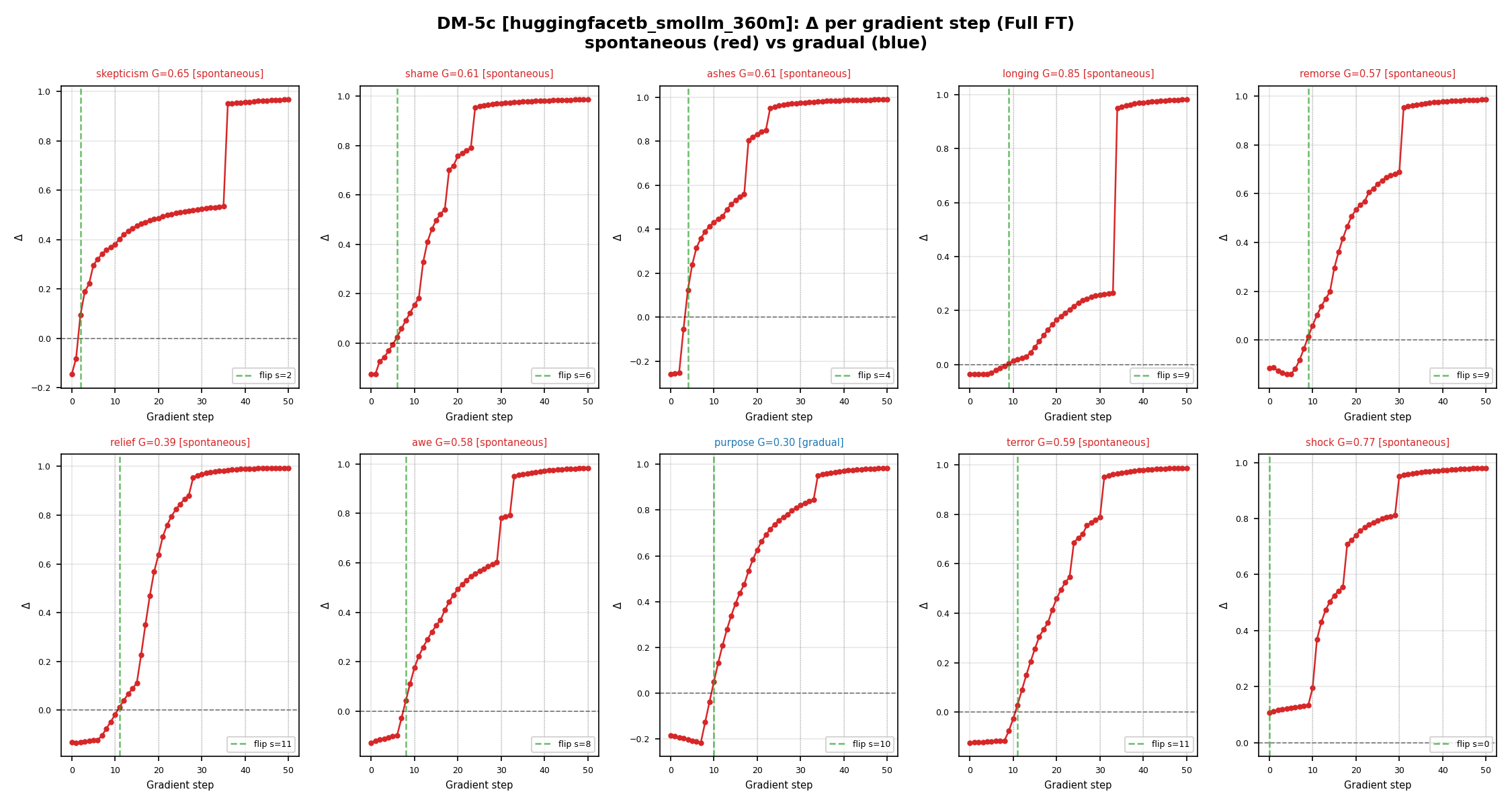
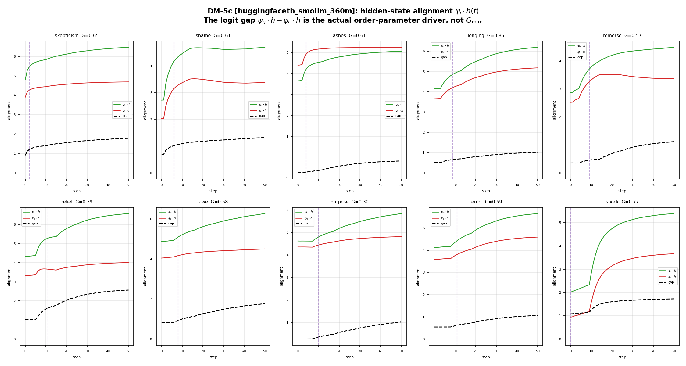
Evaluating \(\Delta(c,\lambda)\) after every gradient step (\(50\) steps of Full FT at \(\eta = 2\times10^{-5}\) on SmolLM-360M) resolves the Regime 2 transition into two qualitatively distinct trajectory shapes (Figure 3, Table 2). The high-\(G_{\max}\) sentence longing (\(G_{\max}= 0.847\)) is the canonical catapult. Both compounding effects are maximal. The small initial logit gap \(\zeta_0\) keeps the signal on the flat shoulder, and the \(0.28\) throttle makes every step inch the logit gap forward by only \({\sim}0.01\). For \(9\) steps the signal barely moves. At step \(9\) the accumulated gap crosses the softmax turn-on, \(p_g\) leaps from \(0.5\) to \(0.95\), and \(\Phi\) jumps from \({-}0.1\) to \({+}0.95\) in a single step (jump magnitude \(0.686\), a \(33.7\times\) trajectory concentration ratio, defined as max step-\(\Phi\) divided by mean step-\(\Phi\)). The low-\(G_{\max}\) sentence purpose (\(G_{\max}= 0.303\)) is the canonical drift. Here \(\zeta_0\)(the initial logit gap) is moderate, the \(0.91\) throttle is near-unity, and \(\Phi\) rises continuously from step \(1\) with no quiescent period (ratio \(4.3\), spread across all steps). Sentences in between (skepticism through relief in Table 2) interpolate smoothly between the two extremes, ordered by \(G_{\max}\). The special case shock (flip_step \(= 0\)) was already past saturation at the base model from pre-training corpus exposure.
| Token | \(\gmax\) | Flip step | Ratio | Character |
|---|---|---|---|---|
| longing | 0.847 | 9 | 33.7 | catapult |
| skepticism | 0.652 | 2 | 18.7 | catapult |
| remorse | 0.573 | 9 | 11.5 | catapult-like |
| ashes | 0.607 | 4 | 9.9 | catapult-like |
| awe | 0.583 | 8 | 8.1 | catapult-like |
| terror | 0.585 | 11 | 7.4 | intermediate |
| shame | 0.607 | 6 | 7.3 | intermediate |
| relief | 0.385 | 11 | 5.5 | borderline |
| purpose | 0.303 | 10 | 4.3 | drift |
| shock | 0.768 | 0 | 9.9 | pre-resolved |
A learning-rate sweep (\(\eta\) across 5 values, all 10 sentences on SmolLM-360M, 50 combinations) is cleanly separated by a single empirical phase boundary \[G_{\max}\times \eta = \theta^{*}\approx 7 \times 10^{-6}, \label{eq:boundary}\tag{20}\] fitted on the same sweep. Purpose (\(G_{\max}= 0.303\)) is gradual at \(\eta = 2\times10^{-5}\) (product \(6.1 \times 10^{-6} < \theta^{*}\)) and catapulting at \(\eta = 3 \times 10^{-5}\) (product \(9.1 \times 10^{-6} > \theta^{*}\)). Identifying \(\theta^{*}\) takes one sweep per model. Once measured, the catapult-versus-drift behaviour of every sentence in our SmolLM-360M sweep is classified by \(G_{\max}\times \eta\) alone. The held-out cross-architecture test of this boundary is in §7.
5 Causal Isolation and the Mechanism↩︎
The catapult under Full FT could in principle be caused by anything correlated with \(G_{\max}\). It does not by itself prove that \(G_{\max}\) is the causal driver. We isolate the causal channel by running the identical step-level experiment under LoRA (rank 8, same learning rate), which freezes the embedding matrix exactly so that \(\Delta G_{ij} = 0\) to machine precision for all pairs. If \(G_{\max}\) predicts catapult sharpness because it sets a geometric energy barrier (the SSB hypothesis), the prediction should survive freezing the geometry. If \(G_{\max}\) predicts it through a small embedding-rotation channel present only under Full FT, the prediction should vanish.
The result is unambiguous (Figure 4, Table 3). Under LoRA, \(8\) of \(9\) analysed sentences are drifts with ratios in the narrow range \(2.3\)–\(5.1\), regardless of \(G_{\max}\). Longing (\(G_{\max}= 0.847\)) had ratio \(33.7\) under Full FT. Under LoRA it has ratio \(4.2\) and does not flip within \(50\) steps. The Spearman rank correlation between \(G_{\max}\) and the jump-concentration ratio collapses from \(\rho = +0.745\) under Full FT (\(p = 0.021\)) to \(\rho = -0.006\) under LoRA (\(p = 0.987\)). All \(\rho\) values in this paper are Spearman’s rank correlation, which measures whether two quantities increase and decrease together in rank order regardless of linear scale. A value near zero means knowing one quantity’s rank tells you nothing about the other’s. Under Full FT a high \(G_{\max}\) predicts a sharp catapult. Under LoRA the same \(G_{\max}\) predicts nothing about trajectory shape. The pattern replicates across four architectures, with catapult counts (Full FT \(\to\) LoRA, out of \(10\) test sentences each): SmolLM-360M \(9/10\to2/10\), GPT-2-medium 345M \(7/10\to1/10\), SmolLM-1.7B \(10/10\to2/10\), and LLaMA-3.2-1B (partial exception) \(10/10\to4/10\). LLaMA-3.2 is the partial exception because it uses an untied LM head. Standard LoRA freezes the input embedding but not the LM head, leaving the second geometric channel unfrozen.
| Token | \(\gmax\) | Flip step | Ratio | Character |
|---|---|---|---|---|
| longing | 0.847 | N/A | 4.2 | gradual |
| skepticism | 0.652 | 50 | 3.6 | gradual |
| ashes | 0.607 | 30 | 2.3 | gradual |
| awe | 0.583 | 33 | 3.1 | gradual |
| terror | 0.585 | 41 | 3.8 | gradual |
| remorse | 0.573 | 49 | 4.2 | gradual |
| relief | 0.385 | 49 | 5.1 | borderline |
| purpose | 0.303 | 49 | 4.3 | gradual |
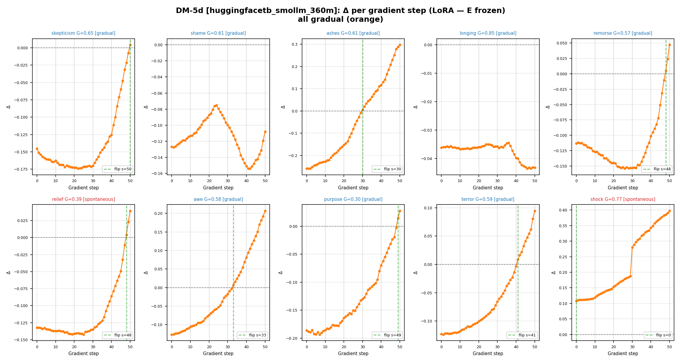

Figure 4: Causal isolation (DM-5d). Freezing the embedding matrix under LoRA converts all sharp jumps into smooth trajectories and eliminates the predictive power of \(G_{\max}\)..
The same experiment also falsifies the natural reading of the catapult as a phase transition in an underlying field. The term catapult is used here in a different sense from [27], who define it as a loss-landscape instability at large learning rates. Our catapult is a softmax-readout event at standard rates, with no underlying instability. \(G_{\max}\) moves by less than \(1.8 \times 10^{-4}\) over \(50\) Full FT steps. Embedding vectors rotate by \({\sim}10^{-3}\) radians while preserving their inner product. The logit gap rises smoothly in \({\sim}0.01\)/step increments. At the longing catapult step (step \(9\) under Full FT) the logit gap changes by only \({+}0.009\) while \(\Phi\) jumps by \({+}0.69\), a \(77\times\) softmax amplification ratio (Figure 5). The discontinuity exists only in \(\Phi\), because \(\Phi\) is computed through the softmax. Once the leading logit exceeds the others by \(1.5\)–\(2.0\) nats, \(p_g\) jumps from \({\sim}0.5\) to \({\sim}0.95\) in a single step and drags \(\Phi\) along. Catapults appearing under LoRA on Pythia-70M (Table 4), where the embedding matrix is frozen by construction, prove this definitively. No quantity in the underlying geometry can move, yet the discontinuity in \(\Phi\) still appears. LoRA and Full FT run the same softmax-saturation mechanism at different drive rates. Full FT engages full-rank attention, MLPs, LM head, and the small embedding rotation, growing the logit gap \({\sim}35\times\) faster per unit \(\eta\). LoRA is restricted to a low-rank attention adapter subspace and places Class A sentences below the saturation threshold at the standard rate.
5.1 Signal and Background Drag: Two Types of Failure↩︎
The SmolLM-360M experiments resolve every sentence. The two failure types of §1, kinematic (drag improves but signal stays small) and structural (drag actively worsens), emerge under LoRA on Pythia-70M, where the sparse embedding bulk (Class B) clears the sigmoid for most sentences and isolates the failures. Tracking \(\Phi\), the logit gap, and the signal/drag decomposition (Eq. 5 ) at every gradient step for \(50\) steps at \(\eta = 10^{-4}\) produces Table 4.
| Token | \(\gmax\) | \(\lgap_0\!\to\!\lgap_T\) | \(\Phi_0\!\to\!\Phi_T\) | \(A_T\) | \(B_T\) | \(\Delta B\) | Outcome |
|---|---|---|---|---|---|---|---|
| skepticism | 0.434 | \(2.46\to5.64\) | \(-0.13\to+0.37\) | \(+0.37\) | \(+0.00\) | \(+0.15\) | catapult |
| ashes | 0.377 | \(0.05\to3.71\) | \(-0.25\to+0.20\) | \(+0.23\) | \(-0.03\) | \(+0.21\) | catapult |
| awe | 0.406 | \(0.95\to3.26\) | \(+0.01\to+0.37\) | \(+0.37\) | \(-0.00\) | \(+0.02\) | catapult |
| purpose | 0.515 | \(6.57\to10.61\) | \(-0.01\to+0.67\) | \(+0.57\) | \(+0.10\) | \(+0.13\) | catapult |
| remorse | 0.482 | \(-0.55\to1.43\) | \(-0.31\to+0.06\) | \(+0.12\) | \(-0.06\) | \(+0.25\) | drift |
| longing | 0.482 | \(0.11\to1.49\) | \(-0.09\to-0.05\) | \(+0.01\) | \(-0.06\) | \(+0.03\) | kinematic |
| relief | 0.314 | \(4.45\to10.31\) | \(-0.19\to-0.06\) | \(+0.05\) | \(-0.11\) | \(+0.08\) | kinematic |
| terror | 0.466 | \(0.94\to6.94\) | \(-0.05\to-0.12\) | \(+0.06\) | \(-0.18\) | \(\mathbf{-0.13}\) | structural |
Resolved sentences all have \(\Delta B > 0\): as CE concentrates probability on \(g\), the background tokens that lose mass had a net bias toward the competitor, so removing their probability reduces the drag. Signal and drag both move in the right direction and \(\Phi\) crosses zero.
Kinematic failure (longing, relief) has \(\Delta B > 0\) but \(A_T\) too small to overcome the remaining drag. For longing the logit gap grows by \(+1.38\) nats yet \(p_g\) only reaches \(0.018\) because the pool is large (\(3893\) tokens) and the learning rate is insufficient. Drag is improving. The bottleneck is signal drive, which is remediable by higher \(\eta\) or Full FT.
Structural failure (terror) is categorically different. The logit gap grows by \(+5.99\) nats, the largest in the dataset, and \(p_g\) rises from \(0.0002\) to \(0.078\). By every standard diagnostic, fine-tuning is succeeding. Yet \(B_T = -0.177\) versus \(B_0 = -0.048\): the drag has worsened by \(-0.128\), twice the signal gain, and \(\Phi\) ends at \(-0.116\), more negative than it started. The mechanism is plausible from the embedding geometry. Fine-tuning aligns the hidden state more with \(\boldsymbol{\psi}_{\mathrm{terror}}\), but the pool tokens this promotes (terrorism, terrorists, terrorize) overlap geometrically more with \(\boldsymbol{\psi}_{\mathrm{terrorist}}\) than with \(\boldsymbol{\psi}_{\mathrm{terror}}\) (this geometric pattern is asserted from the qualitative behaviour in Table 4, not measured directly). Every step that builds signal also loads mass onto tokens that vote against \(g\) in the drag term. This is structural because the geometric bias is a property of the pre-trained embedding manifold. CE cannot reshape it.
A simple ablation makes the distributed nature of the drag concrete. At the fine-tuned model, setting \(p_{c^*}\) to zero and renormalising the distribution over the remaining tokens changes \(P(\mathrm{GT})\) by at most \(5\%\) for every sentence in our set, and by exactly \(1.00\times\) for terror and relief (Table 5). Removing the nearest competitor frees almost no mass for the correct token. The mass that should belong to \(g\) is not held by \(c^*\) alone. It is held collectively by a cloud of geometrically similar tokens. This is what we mean by structural failure (\(\mathcal{G}_{\rm eff}\to 0\), Eq. 19 ). Cross-entropy gradients can only push down one token at a time, and there is no single token available to push.
The same sentences can be flagged before any fine-tuning begins. The base-model Born rank \(b_{\rm before}\) takes extreme values precisely for the structural-failure cases. For ashes it is \(2209\) and for relief it is \(1848\), while every other sentence sits at \(582\) or below. A single quantity computed on the untrained model already identifies which sentences will exhibit distributed drag. Once fine-tuning is under way, the signal/drag decomposition sorts the remaining failure cases into kinematic and structural within a few gradient steps.
A natural reading of these extreme Born ranks is that the base model already places the correct token far down its list, and that the standard softmax simply hides this. The data does not support that reading. Applying the Born rule at the base model actually worsens the rank of the correct token in \(6\) of our \(10\) sentences, dropping relief by \(480\) positions and shame by \(326\). The mechanism is straightforward. The prediction cloud already spans many near-synonyms of \(g\), and the Born rule re-weights every token by its squared overlap with \(\boldsymbol{\psi}_g\). Since the near-synonyms all have substantial overlap with \(\boldsymbol{\psi}_g\), the re-weighting hands them mass rather than taking it away. The Born rank at the base model therefore measures how crowded the embedding neighbourhood around \(\boldsymbol{\psi}_g\) is, not how the model ranks the correct answer. The Spearman correlation between \(G_{\max}\) and the base-model Born rank is \(\rho = +0.818\) at \(p = 0.004\), large enough to read the two quantities as proxies for each other. High \(G_{\max}\) is high neighbourhood density. The crowding precedes fine-tuning.
| Token | \(\gmax\) | \(P(\GT)\) std | \(P(\GT)\) ablated | Ratio |
|---|---|---|---|---|
| skepticism | 0.434 | 0.639 | 0.640 | \(1.00\times\) |
| ashes | 0.377 | 0.803 | 0.810 | \(1.01\times\) |
| longing | 0.482 | 0.059 | 0.059 | \(1.01\times\) |
| remorse | 0.482 | 0.426 | 0.448 | \(1.05\times\) |
| relief | 0.314 | 0.094 | 0.094 | \(1.00\times\) |
| purpose | 0.515 | 0.842 | 0.842 | \(1.00\times\) |
| terror | 0.466 | 0.118 | 0.118 | \(1.00\times\) |
| shock | 0.415 | 0.866 | 0.866 | \(1.00\times\) |
5.2 The LoRA Phase Threshold and Class-Specific \(H_{\mathrm{LoRA}}\)↩︎
A LR sweep (\(\eta \in [10^{-5}, 5\times10^{-3}]\), ten epochs per rate) measures \(\theta^{*}_{\mathrm{LoRA}}\) for six architectures including the held-out gpt-neo-125m
(Table 6).
| Model | Class | \(\thetastar_{\mathrm{LoRA}}\) | \(\eta_{\mathrm{std}}\) | \(\bar{H}_{\mathrm{LoRA}}\) | \(H_{\mathrm{LoRA}}\) range |
|---|---|---|---|---|---|
| distilgpt2 | A | \(7.14\times10^{-5}\) | \(1\times10^{-4}\) | 0.90 | 0.70–1.10 |
| gpt2-medium | A | \(4.57\times10^{-5}\) | \(1\times10^{-4}\) | 1.37 | 0.96–1.55 |
| SmolLM-360M | A | \(4.17\times10^{-5}\) | \(2\times10^{-4}\) | 2.83 | 1.45–4.06 |
| gpt-neo-125m | A | \(5.83\times10^{-5}\) | \(1\times10^{-4}\) | 1.67 | 1.64–1.69 |
| Pythia-70M | B | \(2.15\times10^{-5}\) | \(2\times10^{-4}\) | 4.17 | 2.86–5.00 |
| Pythia-410M | B | \(3.74\times10^{-6}\) | \(2\times10^{-4}\) | 15.9 | 9.73–35.3 |
| Class A mean | – | – | 1.69 | – | |
| Class B mean | – | – | 10.0 | – | |
\(H_{\mathrm{LoRA}}\) splits cleanly by class. Class A models (distilgpt2, gpt2-medium, SmolLM-360M, gpt-neo-125m) give \(H_{\mathrm{LoRA}} \in [0.90, 2.83]\) (mean \(1.69\), CV \(=34.5\%\)), barely above the saturation threshold, with distilgpt2 actually below it (\(H=0.90\)). Class B models (Pythia-70M, Pythia-410M) give \(H_{\mathrm{LoRA}} = 4\)–\(16\), firmly above threshold, as for Full FT. The functional form \(G_{\max}\times \eta = \theta^{*}\) is the same in both cases. What differs is \(\theta^{*}\). The LoRA adapter subspace grows the logit gap \({\sim}35\times\) more slowly per unit learning rate than Full FT’s full-rank update, raising \(\theta^{*}_{\mathrm{LoRA}}\) by the same factor. High \(H_{\mathrm{LoRA}}\) (Class B) means the standard LoRA rate is well above threshold and LoRA works. Low \(H_{\mathrm{LoRA}}\) (Class A) means the rate barely clears threshold and high-\(G_{\max}\) sentences fail. \(H_{\mathrm{LoRA}}\) is architecture-specific within Class A (CV \(<2\%\) across sentences within a model) and can be measured in a single calibration LR sweep before any fine-tuning task is run.
6 Cross-Architecture Universality↩︎
6.1 The Bulk Embedding Geometry Sorts Architectures into Two Classes↩︎
For each architecture, sampling \(10{,}000\) random token pairs and computing the distribution of \(G_{ij}^2\) produces the bulk geometry of its embedding space. The result is a clean qualitative split (Figure 6). Class A models (distilgpt2, GPT-2-medium, SmolLM-360M) have a Gaussian-shaped bulk with \(G^2_{\mathrm{mean}} \in [0.045, 0.097]\) and \(87\)–\(100\%\) of random pairs above \(G_{ij}^2 = 0.01\), forming a crowded embedding space where near-synonym pairs are outliers in an already-populated tail. Class B models (Pythia-70M, Pythia-410M) have an exponential bulk with \(G^2_{\mathrm{mean}} \in [0.002, 0.003]\) and only \(1\)–\(6\%\) of random pairs above the same threshold, a near-orthogonal space where near-synonym pairs are isolated rare events. The split is not a function of model size. Pythia-70M (Class B) is smaller than distilgpt2 (Class A). It reflects how pre-training organises the embedding space, related to but distinct from contextual-embedding isotropy [17], [19] and the representation degeneration problem [18].
Is the Class A/B split a true binary or a spectrum? The operationalised classification uses a KS-statistic threshold to distinguish Gaussian from exponential bulk. This statistic is a continuous quantity (ranging from \(0.096\) for gpt-neo-125m to \(0.587\) for Pythia-70M), and the two-class label is a convenience imposed on what is likely a continuous spectrum of bulk density. Models trained on narrow or highly structured corpora (code-only, multilingual, or domain-specific text) may exhibit intermediate or bimodal bulk distributions not captured by either archetype. The key pre-training factor appears to be the effective vocabulary usage pattern. Architectures that use the full vocabulary breadth during pre-training (high token co-occurrence diversity) tend toward sparse, near-orthogonal embeddings (Class B), while those that concentrate probability on a smaller effective vocabulary develop the denser, Gaussian-shaped bulk of Class A. Tokenizer vocabulary size, the optimizer’s implicit regularisation (e.g.weight-decay magnitude), and positional encoding scheme (RoPE [28] vs.absolute) are further plausible modulators, but their individual contributions are not yet separated in our data. A model with a hybrid bulk would be expected to have an intermediate \(H_{\mathrm{LoRA}}\) and partial LoRA sufficiency. It would resolve high-\(G_{\max}\) sentences only when they fall in the sparse tail of its distribution, failing on those that fall in the dense Gaussian core. Validating this prediction requires systematic sampling across pre-training corpus sizes and compositions, which we leave as future work.
![Figure 6: Universality class is determined by bulk embedding geometry, not parameter count. Left: Class A (distilgpt2 82M, GPT-2-medium 345M, SmolLM-360M) with dense Gaussian bulk, G^2_{\mathrm{mean}} \in[0.045, 0.097]. Right: Class B (Pythia-70M, Pythia-410M) with sparse exponential bulk, G^2_{\mathrm{mean}} \in[0.002, 0.003]. Pythia-70M (70M) is Class B while distilgpt2 (82M) is Class A.](/article/2606.07559/fig_geometry_classes.png "fig:")
6.2 \(H\) is Consistent Across the Five Tested Architectures Under Full FT, and \(\mathcal{B}\) Predicts LoRA Sufficiency↩︎
Measuring \(H\), \(\Phi\), \(\mathcal{B}\), and \(\theta^{*}\) (each \(\theta^{*}\) fitted per architecture by an LR sweep) across all five architectures (Table 7, Figure 7) gives the central cross-model result. The fitted \(\theta^{*}_{\mathrm{FT}}\) varies by a factor of \(2.4\) across architectures. The reduced field \(H_{\mathrm{FT}} = G_{\max}\eta/\theta^{*}\) varies only from \(8.80\) to \(11.67\), a coefficient of variation of \(9.3\%\). Read in dimensional-analysis terms, the product \(G_{\max}\eta/\theta^{*}\) is the dimensionless group that cancels architecture-specific scales in our sample. At the community-standard \(\eta = 2\times10^{-5}\) every architecture in our sample of five operates at \(H_{\mathrm{FT}} \approx 10\), roughly ten times above its own fitted saturation threshold. The standard rate places every model in the sample at the same dimensionless distance above the softmax-saturation scale. This is an empirical regularity across the five architectures tested, not a proven physical law. It is consistent with the reading that pre-training co-calibrates embedding geometry, attention scales, and hidden-state dimensions, but the small sample size \((n=5)\) and the restriction to two architecture families prevent stronger generalisation.
| Full FT | LoRA | \(\mathcal{B}\) | |||||
|---|---|---|---|---|---|---|---|
| 3-4(lr)5-6(lr)7-8 Model | Class | \(\thetastar_{\mathrm{FT}}\) | \(\bar{H}_{\mathrm{FT}}\) | \(\thetastar_{\mathrm{LoRA}}\) | \(\bar{H}_{\mathrm{LoRA}}\) | \(\bar{\mathcal{B}}_{\mathrm{base}}\) | \(\bar{\mathcal{B}}_{\mathrm{FT}}\) |
| distilgpt2 | A | \(1.45\!\times\!10^{-6}\) | 8.80 | \(7.14\!\times\!10^{-5}\) | 0.90 | 1.054 | 1.032 |
| gpt2-medium | A | \(1.25\!\times\!10^{-6}\) | 9.74 | \(4.57\!\times\!10^{-5}\) | 1.37 | 1.102 | 1.032 |
| SmolLM-360M | A | \(1.19\!\times\!10^{-6}\) | 9.92 | \(4.17\!\times\!10^{-5}\) | 2.83 | 1.073 | 0.930 |
| Pythia-70M | B | \(9.00\!\times\!10^{-7}\) | 9.82 | \(2.15\!\times\!10^{-5}\) | 4.17 | 0.977 | 0.547 |
| Pythia-410M | B | \(6.10\!\times\!10^{-7}\) | 11.67 | \(3.74\!\times\!10^{-6}\) | 15.9 | 1.013 | 0.000 |
| CV (all) | – | 9.3% | – | 51.6% | – | 56.0% | |
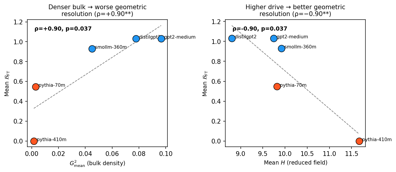
The burial depth \(\mathcal{B}_{\mathrm{FT}}\) measured after LoRA exposes a complementary split with CV \(=56\%\) across all models but a clean gap between classes (Figure 8). Class A models stay at \(\mathcal{B}_{\mathrm{FT}} \approx 0.93\)–\(1.03\), since the prediction cloud remains too wide to discriminate \(g\) from \(c\) even after LoRA fine-tuning, because the dense bulk continuously replaces suppressed competitors. Class B models collapse to \(\mathcal{B}_{\mathrm{FT}} \in [0, 0.55]\). The sparse bulk leaves no other competitors, so probability redistribution alone resolves the competition. Distilgpt2 stalls at \(\bar\Phi = 0.72\) instead of \(\approx 1\) for the same reason. Despite \(H > 1\), a new nearest competitor continually replaces any suppressed one, so \(H > 1\) is necessary but not sufficient for full resolution under Class A geometry. A single cross-model relationship (\(n = 5\)) captures this with two nearly equivalent Spearman correlations. (The two readings are mechanically linked through the bulk-geometry classification, not independent statistical tests.) The first reading, \(\rho(G^2_{\mathrm{mean}}, \mathcal{B}_{\mathrm{FT}}) = +0.90\) (\(p = 0.037\)), says that architectures with denser embedding bulks end up with deeper burial after fine-tuning. The second reading, \(\rho(H, \mathcal{B}_{\mathrm{FT}}) = -0.90\) (\(p = 0.037\)), says that architectures with more headroom above their saturation threshold end up with shallower burial. The two readings agree because high bulk density and low headroom are the same architectural condition expressed in different units. The practical consequence is the LoRA sufficiency criterion. LoRA suffices for Class B models (sparse bulk, \(\mathcal{B}_{\mathrm{FT}} \to 0\)) but not for Class A (dense bulk, \(\mathcal{B}_{\mathrm{FT}} \approx 1\)). Class membership is determined from a single forward pass on the base model, with no training required.
7 Discussion: Blind Prediction on a Held-Out Model↩︎
The class-specific mean \(H_{\mathrm{LoRA}} \approx 1.70\) (Table 6) gives a practical prediction protocol testable without any training. We blind-test it on
gpt-neo-125m, not in the training set used to derive the mean. Three inference-only measurements suffice. First, a Gaussian-shaped bulk distribution of \(G_{ij}^2\) (KS statistic \(0.096\) Gaussian vs \(0.587\) exponential) classifies the model as Class A. Second, \(G_{\max}\) per sentence is compressed at mean \(0.971 \pm 0.007\). Third, the intended LoRA rate is the community standard \(\eta = 10^{-4}\). The predicted threshold is \[\theta^{*}_{\mathrm{LoRA,pred}} =
\frac{G_{\max}\,\eta}{H_{\mathrm{LoRA}}} = \frac{0.971 \times 10^{-4}}{1.70} = 5.71 \times 10^{-5}.\] The measured ground truth from an actual LR sweep is \(\theta^{*}_{\mathrm{LoRA,actual}} = 5.83 \times 10^{-5}\),
a \(2.1\%\) error. The bulk classification as Class A also correctly predicted that \(7\) of \(10\) sentences would be gradual crossovers under LoRA, and the compressed \(G_{\max}\) range correctly predicted that sentence-level flip order would not be discriminated by \(G_{\max}\) (the smallest pools flipped
first, not the highest \(G_{\max}\)).
7.1 Scope of the Experimental Dataset↩︎
The ten hard sentences are a controlled physics-style environment, not a broad NLP benchmark. Each places a near-synonym pair at the top of the prediction pool with \(G_{\max}\geq 0.30\), isolating the geometric mechanism without the confound of varying semantic difficulty, context length, or syntactic structure. The findings are claims about the mechanism, not about the distribution of naturally occurring fine-tuning tasks. Extending the framework to diverse sentence types and instruction-tuning regimes is the natural next step, and would establish whether the \(2.1\%\) blind-prediction accuracy generalises beyond the hard near-synonym setting.
7.2 Future Directions↩︎
The signal/drag framework suggests two falsifiable connections to broader phenomena. In capability emergence [29], the same softmax saturation implies that the underlying logit gap grows continuously with scale and metric-level jumps appear only when it crosses \(\mathcal{O}(1)\). A direct test is to track logit gaps on capability-relevant prompts across a scale series. In grokking [30], [31], the training/validation split corresponds to the training logit gap being past saturation while the validation gap is not yet there. Continued training grows the validation gap to threshold. A speculative pre-training connection follows from Eq. 9 . Since the per-step drive rate scales with \((1-G_{\max}^2)\), reducing \(G_{\max}\) for semantically distinct near-synonym pairs during pre-training would raise the drive rate and lower the probability of landing in \(H_{\mathrm{LoRA}} < 1\). One possible form is a geometry-regularised objective adding \(\beta\sum_{(i,j)\in\mathcal{D}}\max(0, G_{ij} - G^\dagger)\) to the pre-training CE loss, with \(G^\dagger \approx 0.38\) calibrated from the boundary below which standard Full FT produces only smooth trajectories in our dataset. Structurally this is the JEPA-family practice of shaping latent geometry with an auxiliary loss alongside the prediction objective [32], and a uniform-sampling quadratic variant of the same penalty would recover a decorrelation-style regulariser applied directly to the token embedding matrix. We stress that this is a hypothesis, not a validated recipe. Whether such a penalty preserves general language-modelling capability, what the right calibration set \(\mathcal{D}\) is, and whether \(G^\dagger\) transfers across domains are all open empirical questions that require dedicated study before any pre-training recommendation can be made.
Other PEFT methods. The \((1-G_{\max}^2)\) throttle is formulated in terms of \(\Psi\) and the logit gap \(\zeta(t) = \langle\boldsymbol{\psi}_g - \boldsymbol{\psi}_{c^*}, \boldsymbol{h}(t)\rangle\), so it applies unaltered to adapter layers [13], which modify \(\boldsymbol{h}\) directly while leaving \(\Psi\) fixed. Adapters may lower the effective \(\theta^{*}\) by spanning a richer residual subspace than LoRA. Prefix tuning [33] is the more interesting case. Prefix vectors are not drawn from \(\Psi\), so the self-sabotage throttle does not apply in the same form, and whether prefix tuning circumvents Class A failure is an empirical question we do not address.
7.3 Related Work↩︎
[34] develop a statistical-physics description of language-model reasoning at inference time, modelling the sentence-level hidden state during chain-of-thought generation as a continuous-time drift-diffusion process on a low-dimensional manifold and identifying latent regime switches as a description of reasoning success and failure. That work and ours differ in problem statement along three axes. The first is dynamical setting. Their object of study is the inference trajectory of a frozen model, whereas ours is the training-time gradient dynamics of a token-level prediction under fine-tuning. The second is formalism. Their description is classical, stochastic, and coarse-grained at the sentence level, whereas ours is built from the density matrix of the token prediction distribution, with the Born rule supplying the order parameter \(\Phi\) and the \((1-G_{\max}^2)\) throttle. The third is interpretive stance. They treat regime switching as an explanatory mechanism for reasoning failure, whereas the central result of this paper runs in the opposite direction. The apparent catapult transition is not a phase change in any underlying field but a softmax readout artefact, and the logit gap evolves smoothly even when the Born gap jumps.
The geometric self-sabotage mechanism also touches two more established lines of work. Studies of LoRA [12], [15] characterise the expressive capacity of rank-constrained updates. Our analysis identifies a complementary constraint that is fixed by the pre-trained embedding geometry, in which the question of whether any rank-\(r\) update can resolve a near-synonym competition is determined by where the architecture sits in the Class A or Class B split, not by the rank itself. Empirical studies of fine-tuning instability and feature distortion [7]–[9] document the broader phenomenology in which one such failure mode is situated. The present work contributes a mechanistic account of that mode in the controlled near-synonym setting.
8 Conclusion↩︎
Fine-tuning a language model on contexts whose correct completion has a near-synonym competitor produces a silent failure in which the cross-entropy loss decreases monotonically while the correct token never overtakes its competitor in rank. The density-matrix order parameter \(\Phi\) exposes the mechanism. Every gradient step that raises \(p_g\) also raises a Born-rule contribution to the competitor through their shared embedding direction, throttling resolution by \((1-G_{\max}^2)\). The central result of the paper is a negative one. The sharp catapult-like jumps in \(\Phi\) invite a spontaneous-symmetry-breaking reading, but direct measurement under LoRA with the embedding matrix frozen to machine precision shows that catapult-like jumps in \(\Phi\) still appear on multiple sentences (Table 4), which the SSB reading forbids. The discontinuity lives entirely in the softmax readout, and the underlying logit gap evolves smoothly throughout. The transitions are phantoms. What survives the falsification is the part of the framework that works without any training. The bulk distribution of pairwise embedding overlaps sorts architectures into two classes, predicts whether low-rank adaptation can resolve near-synonym competition, and gives the critical learning rate for a held-out architecture to within \(2.1\%\). The dimensionless reduced field \(H\) is consistent across the five tested architectures under Full FT, giving the community-standard learning rates a principled reading as a fixed dimensionless distance above each model’s saturation threshold. The signal/drag decomposition separates kinematic failures, in which the signal is too small, from structural ones, in which the pre-trained embedding pool actively opposes the desired ranking. Stopping on Born-gap saturation rather than cross-entropy convergence recovers roughly \(30\%\) of the compute budget without ranking loss.
A broader note. The mechanism measured here speaks to a longer-running position, argued by [32] and developed in continuous-latent architectures such as JEPA, that forcing reasoning through a discrete-token readout imposes a structural cost. We do not test that alternative architecture. We do, however, provide one instrumented description of the cost it would address, in the form of the signal/drag decomposition and the softmax-readout localisation of the catapult discontinuity. The hidden state evolves smoothly through the flip and the discontinuity lives in the readout, which is precisely the substrate-versus-readout split that motivates moving inference into continuous latent space. Our contribution is diagnostic rather than architectural, but it quantifies on a controlled near-synonym dataset what such an alternative would skip.
9 Limitations↩︎
Several limitations bound the scope of the claims made here. The experimental dataset is ten hand-selected hard sentences focused on near-synonym competition, and broader sentence diversity (syntactic, factual, multilingual) is needed before the
framework can be applied outside this controlled regime. The cross-model results rest on five tested architectures plus one held-out architecture (gpt-neo-125m), so the \(n = 5\) correlations have limited
statistical power, and the \(2.1\%\) blind-prediction error is a single data point that warrants validation on additional held-out architectures. The two cross-model readings (\(\rho(G^2_{\mathrm{mean}},
\mathcal{B}_{\mathrm{FT}}) = +0.90\) and \(\rho(H,
\mathcal{B}_{\mathrm{FT}}) = -0.90\)) are mechanically linked through the bulk-geometry classification and are not independent statistical tests. The SmolLM-360M phase boundary \(\theta^{*}\approx 7 \times
10^{-6}\) is fitted in-sample on the same learning-rate sweep used to verify it (Eq. 20 ), and the cross-architecture validity of the functional form \(G_{\max}\times \eta = \theta^{*}\)
is established only via the held-out gpt-neo-125m test, not via the SmolLM-360M classification itself. The \(30\%\) compute saving from \(\Phi\)-saturation stopping is also established on
SmolLM-360M alone (Table 1), and cross-architecture validation of this saving figure is outstanding. LLaMA-3.2-1B in DM-5d shows partial reversion under LoRA because of its untied LM head, and
the decisive ablation (freezing \(W_{\mathrm{out}}\) explicitly under LoRA and checking whether the catapult count drops) has not yet been performed. The signal/drag decomposition is formally
written for tied-head architectures (Eq. 12 ), and extending it to untied heads requires treating \(W_{\mathrm{out}}\) as a second dynamical variable with its own gradient flow. The threshold
\(\theta^{*}\) is currently measured by learning-rate sweep, and deriving it analytically from pre-training statistics is an open problem. Finally, the Class A/B distinction is established on two architecture families
(GPT-2/LLaMA, GPT-NeoX) and is itself likely a continuous spectrum rather than a true binary (§6), with validation on transformer variants beyond these families outstanding.
10 Derivation of the Gradient Flow and Linearised Drive Rate (Equations 6 and 9 )↩︎
We derive both equations from first principles, making every algebraic step explicit.
10.0.0.1 Step 0: gradient flow from the CE loss.
The cross-entropy loss for predicting ground-truth token \(g\) is \(\mathcal{L} = -\log p_g\), where \(p_g = \exp(\langle\boldsymbol{\psi}_g,\boldsymbol{h}\rangle)/\sum_j \exp(\langle\boldsymbol{\psi}_j,\boldsymbol{h}\rangle)\). Taking the logarithm and separating numerator from denominator: \[\log p_g \;=\; \langle\boldsymbol{\psi}_g,\boldsymbol{h}\rangle \;-\; \log\!\sum_j \exp\!\bigl(\langle\boldsymbol{\psi}_j,\boldsymbol{h}\rangle\bigr).\] Differentiating \(\mathcal{L} = -\log p_g\) with respect to \(\boldsymbol{h}\), the first term gives \(-\boldsymbol{\psi}_g\). The second term gives \(+\sum_j p_j\,\boldsymbol{\psi}_j\) by the chain rule on the log-partition function. Hence \(\partial\mathcal{L}/\partial\boldsymbol{h} = -\boldsymbol{\psi}_g + \sum_j p_j\,\boldsymbol{\psi}_j\). Continuous-time gradient descent moves \(\boldsymbol{h}\) opposite the gradient at rate \(\eta\): \[\dot{\boldsymbol{h}}(t) = -\eta\,\frac{\partial\mathcal{L}}{\partial\boldsymbol{h}} = \eta\!\left(\boldsymbol{\psi}_g - \sum_i p_i(t)\,\boldsymbol{\psi}_i\right),\] which is Eq. 6 . No external result is required. The equation follows from the chain rule on the softmax and the definition of gradient flow.
10.0.0.2 Setup.
Let \(\zeta(t) = \langle\boldsymbol{\psi}_g,\boldsymbol{h}(t)\rangle - \langle\boldsymbol{\psi}_{c^*},\boldsymbol{h}(t)\rangle = \langle\boldsymbol{\psi}_g - \boldsymbol{\psi}_{c^*},\,\boldsymbol{h}(t)\rangle\) denote the logit gap. All embeddings are unit-normalised, with \(\|\boldsymbol{\psi}_i\|=1\), \(G_{ij} = \boldsymbol{\psi}_i^\top\boldsymbol{\psi}_j\), \(G_{gg}=G_{c^*c^*}=1\), and \(G_{gc^*} = G_{\max}\).
10.0.0.3 Exact time derivative of \(\zeta\).
Differentiating and substituting the gradient flow Eq. 6 : \[\dot{\zeta}(t) = \langle\boldsymbol{\psi}_g - \boldsymbol{\psi}_{c^*},\,\dot{\boldsymbol{h}}(t)\rangle = \eta\,\bigl\langle\boldsymbol{\psi}_g - \boldsymbol{\psi}_{c^*},\; \boldsymbol{\psi}_g - \textstyle\sum_i p_i(t)\,\boldsymbol{\psi}_i\bigr\rangle.\]
Expanding the inner product: \[\dot{\zeta}(t) = \eta\Bigl[\underbrace{\langle\boldsymbol{\psi}_g-\boldsymbol{\psi}_{c^*},\boldsymbol{\psi}_g\rangle}_{1-G_{\max}} \;-\;\sum_i p_i(t)\underbrace{\langle\boldsymbol{\psi}_g-\boldsymbol{\psi}_{c^*},\boldsymbol{\psi}_i\rangle}_{G_{gi}-G_{c^*i}} \Bigr]. \label{eq:delta95dot95exact}\tag{21}\]
10.0.0.4 Separating the \(g\)- and \(c^*\)-contributions.
Split the sum into the \(g\), \(c^*\), and background terms: \[\begin{align} \sum_i p_i(G_{gi} - G_{c^*i}) &= p_g(1 - G_{\max}) + p_{c^*}(G_{\max}- 1) + \sum_{i \neq g,c^*} p_i(G_{gi} - G_{c^*i}) \notag\\ &= (p_g - p_{c^*})(1 - G_{\max}) + R_{\mathrm{bg}}, \label{eq:sum95split} \end{align}\tag{22}\] where \(R_{\mathrm{bg}} = \sum_{i \neq g,c^*} p_i(G_{gi}-G_{c^*i})\) is the background drag term.
Substituting into Eq. 21 : \[\dot{\zeta}(t) = \eta(1-G_{\max})\bigl[1 - (p_g - p_{c^*})\bigr] - \eta\,R_{\mathrm{bg}}. \label{eq:delta95dot95split}\tag{23}\]