FP8 is All You Need (Part 1):
Debunking Hardware FP64 as the HPC Holy Grail2
A Tensor–Memory Equilibrium Model and Implementation Strategy
for Ozaki Scheme II on Memory-Bound Workloads
in the Post-fp64 Era
May 28, 2026
Abstract
The conventional HPC dogma has long held that native hardware fp64 silicon is the irreducible foundation of scientific computing—the “holy grail” without which credible double-precision simulation is impossible. This paper argues, on the basis of a unified analytic model and a kernel-by-kernel audit, something stronger than its refutation: that the FP8 tensor-core matrix-multiply is the sole computational primitive on which double-precision scientific computing needs to be built. On AI-optimised GPUs of the B300 generation and beyond, abundant fp8 tensor throughput combined with the Chinese Remainder Theorem-based Ozaki Scheme II recovers memory-roof execution at full fp64 accuracy across the entire canonical HPC kernel spectrum; native fp64 silicon is demoted from a hardware requirement to a derived accuracy guarantee produced by composition over the FP8 primitive.
We organise the claim as a compositional hierarchy. At its base (L0) is the FP8 matrix op; one layer up (L1) is the Ozaki II scheme, which composes FP8 multiplies into an exact fp64-accurate product; above it (L2) are the basic numerical kernels—the Berkeley “dwarfs” of dense and sparse linear algebra, spectral transforms, and stencils; then the composite solver kernels that form application inner loops (L3); and finally full scientific applications (L4). The Berkeley dwarfs catalogued the canonical kernels precisely so the field could be reasoned about at the right level of abstraction; this paper closes the question they left open by exhibiting the single hardware primitive onto which the whole taxonomy maps. The only non-FP8 arithmetic anywhere in the stack is a bounded, fixed-width integer accumulation in the reconstruction step.
The central contribution is this structural claim itself; the remainder of the paper exists to establish it. We make the claim falsifiable—it asserts that every dwarf, and every composition of dwarfs, stays on the bandwidth-bound side of the roofline under FP8 emulation—and we build the instrument that tests it: the Tensor–Memory Equilibrium (TME) model, which augments the classical Roofline [1] with three emulation-specific parameters, the compute multiplier \(\alpha=3r{+}1\) (low-precision MMAs per high-precision op), the bandwidth multiplier \(\beta\) (data inflation from residue expansion), and the reconstruction latency \(\gamma\). Within this model we identify register-level fusion as the mechanism that drives \(\beta\!\to\!1\) for streaming kernels—turning “FP8 can emulate FP64” into “FP8 keeps the memory-bound kernels at the memory roof.” We then substantiate the reduction quantitatively: across B300 and Rubin R200, Ozaki II lifts the emulated fp64 ceiling from the collapsed \(\sim\!1.3\) TFLOPS native floor to \(\sim\!135\) TFLOPS (B300) and \(\sim\!108\) TFLOPS (Rubin) at \(r\!=\!12\) with the full \((3r{+}1)\) cost, which reduces the dense compute-bound ceiling but leaves the memory-bound result untouched, since the surveyed memory-bound kernels sit far below the emulation ridge; against the last HPC-balanced GPU (H100) as baseline, every workload on every GPU studied matches or exceeds H100, in contrast to the up-to-\(50\times\) regression native B300 fp64 imposes. Finally, a forward audit of the composite kernels (L3), combined with a companion FFT analysis [2] and FP32+Kahan compensation for reductions, closes the kernel coverage so that every surveyed class reaches the memory roof at full fp64 accuracy.
That the TME model could have returned a negative verdict, yet instead returns a positive one across the dwarfs and their compositions, is the paper’s analytical content. This is, by design, the analytical half of a two-part argument; a follow-on implementation effort validates the thesis on production silicon by realising the kernels and measuring the delivered \((\alpha,\beta)\) end-to-end. We are explicit about the questions the structural claim leaves open—chiefly the composition overhead captured by \(\beta\), together with a small, identifiable set of corner cases—and we concentrate them, with the conditions under which the thesis would be falsified, in a single dedicated section rather than hedging the analysis throughout.
Keywords: FP8 tensor-core emulation; Ozaki Scheme II; Tensor–Memory Equilibrium (TME) model; memory-bound HPC kernels; NVIDIA Blackwell Ultra (B300); post-FP64 GPU architecture; AI for Science (AI4S).
1 Introduction↩︎
The trajectory of high-performance computing (HPC) hardware has bifurcated. While scientific simulation—ranging from Quantum Chromodynamics and Computational Fluid Dynamics to climate emulation and seismic imaging—continues to rely on IEEE 754 double-precision (fp64) arithmetic for numerical stability and reproducibility, the data-center GPU market is decisively pivoting toward Artificial Intelligence. This pivot is characterised by an exponential increase in low-precision throughput (fp16, fp8, fp6, fp4) at the direct expense of native fp64 capability.
The NVIDIA Blackwell architecture [3], [4] serves as the canonical case study. Whereas the B200 retained a respectable \(\sim\!40\) TFLOPS of dense fp64 tensor performance, the Blackwell Ultra B300—based on the same architecture but with tensor cores re-balanced for NVFP4—reports only \(\sim\!1.3\) TFLOPS sparse / \(1.2\) TFLOPS dense fp64 per GPU in the official datasheet [5]. Independent microbenchmark analyses confirm the fp64 regression and document the ascent of NVFP4 to the role of primary tensor format [4], [6], and commentary at SC25 underscored that the platform’s \(64\)-bit floating-point capability does not improve over the previous generation [7].
The successor architecture, NVIDIA’s Vera Rubin platform (R200 GPU), sustains the same trajectory. NVIDIA’s published Rubin specifications report native fp64 vector performance at \(\sim\!33\) TFLOPS—a further regression from B200’s \(\sim\!40\) TFLOPS [8]—and list, for the first time, an explicit “Emulated DGEMM” column at \(\sim\!200\) TFLOPS that is achieved through Ozaki-style emulation [9], [10]. In parallel, Rubin ships with 22 TB/s HBM4 bandwidth—\(2.75\times\) over B300’s 8 TB/s—and 4 PFLOPS of dense fp8 matrix throughput. NVIDIA has thus committed to emulation as the official path to fp64-equivalent matrix performance on its scientific-computing flagship, a commitment made concrete in the next generation of Rubin-based supercomputers now being deployed at major HPC centres [11], [12].
This regression has two consequences that, until now, have not been treated together.
1.0.0.1 Consequence 1: Memory-bound kernels become compute-bound.
The classical Roofline ridge point—the operational intensity at which the compute roof and the memory roof intersect—is given by \(P_{\mathrm{\small fp64}}/B_{\text{mem}}\), where \(P_{\mathrm{\small fp64}}\) is the peak fp64 throughput and \(B_{\text{mem}}\) is the HBM bandwidth. On B300 this ridge sits at \(1.3\,\text{TFLOPS} / 8\,\text{TB/s} = 0.16\) FLOPS/Byte, so low that essentially every dense linear-algebra kernel narrower than a GEMM falls into the compute-bound regime. A 7-point stencil with operational intensity \(\approx 0.5\) FLOPS/Byte should run at the memory roof of \(8 \cdot 0.5 = 4\) TFLOPS, but is instead capped at \(1.3\) TFLOPS by the native fp64 pipe. In other words, the bandwidth that the application needs is physically present on the chip but cannot be consumed by the arithmetic units.
1.0.0.2 Consequence 2: Low-precision tensor units are dormant.
At the same time, the B300 carries 10 PFLOPS of dense NVFP4 throughput (15 PFLOPS sparse) and 5 PFLOPS of dense fp8 (10 PFLOPS sparse). In a typical fp64-only HPC kernel these units are idle, and the silicon area they occupy contributes nothing to the kernel’s time-to-solution. This is the Dark Silicon manifestation of the AI–HPC divergence.
1.0.0.3 The Ozaki Scheme.
The Ozaki scheme [13], originally introduced for accurate dot products and matrix multiplication, has emerged over the last decade as the canonical mechanism for reclaiming this dormant throughput. Recent work has extended the scheme in two directions: the original Ozaki I (mantissa slicing) has been adapted to fp16, fp8 and int8 tensor cores [14], [15], and a fundamentally different Ozaki II variant based on the Chinese Remainder Theorem (CRT) was proposed by Ozaki, Uchino and Imamura in 2025 [16]. NVIDIA integrated Ozaki-style emulation into cuBLAS in October 2025 [17], and the U.S.Department of Energy’s Genesis Mission has explicitly identified Ozaki emulation as its fallback path for fp64-accurate scientific computing on AI-centric hardware [18]. At the same time, AMD’s recent positioning around the MI430X suggests that not every vendor is convinced that emulation alone is sufficient [19].
1.0.0.4 The gap addressed by this paper.
Despite the rapid maturation of Ozaki I and Ozaki II for dense GEMM, all published performance studies have focused on the compute-bound regime where the technique most obviously wins. No published analysis (to our knowledge, as of June 2026) systematically asks: when is Ozaki II profitable for memory-bound kernels? This is the operating regime that dominates real scientific simulation codes: stencil sweeps in PDE solvers, SpMV in iterative linear solvers, batched GEMV in time-stepped reduced-order models, and similar bandwidth-limited primitives. The conventional wisdom—that EFT methods cannot help bandwidth-limited kernels because they inflate operand counts—deserves a more careful look on hardware where the fp64 compute roof has collapsed below the memory roof.
1.0.0.5 Contributions of this paper.
The central contribution of this paper is conceptual, and the technical results exist to establish it:
The “FP8 is all you need” thesis: the FP8 tensor-core matrix-multiply is the sole computational primitive of double-precision scientific computing. We argue—and structure the entire paper around—the claim that every canonical fp64 HPC kernel, and every application that composes them, reduces to sequences of FP8 matrix operations through the Ozaki II scheme, the only non-FP8 arithmetic anywhere in the stack being a bounded, fixed-width integer accumulation in the reconstruction step. Native fp64 silicon is, on this account, not a hardware requirement but a derived accuracy guarantee obtained by composition over the FP8 primitive. This recasts the industry’s fp8-ward shift from a threat to double-precision science into its sufficient foundation.
A compositional hierarchy (L0–L4) that makes the thesis precise and a Berkeley-“dwarfs” argument that makes it complete (§1.1). We organise scientific computing into five layers —the FP8 op (L0), Ozaki II (L1), the basic numerical kernels or “dwarfs” (L2), the composite/solver kernels of real application inner loops (L3), and full applications (L4)—and show that, because the Berkeley dwarf taxonomy already spans scientific computing, exhibiting the reduction of every dwarf to the FP8 primitive establishes the thesis for the whole field by composition rather than by sampling.
The thesis is falsifiable, and we supply the instrument that tests it. We make the claim operational—every kernel must stay on the bandwidth-bound side of the roofline (or remain otherwise fp64-competitive) under FP8 emulation—and develop the Tensor–Memory Equilibrium (TME) model (§4), a Roofline extension exposing the three emulation parameters \((\alpha,\beta,\gamma)\), expressly so the claim could be refuted per kernel. That it instead survives across the dwarfs (L2, §5–6) and their compositions (L3, §7) is the paper’s analytical content.
The mechanism that makes the reduction efficient, not merely possible. We identify register-level fusion as the structural reason the bandwidth multiplier \(\beta\!\to\!1\) for streaming kernels, keeping the residue/reconstruction traffic on-chip so that emulation is essentially free behind the memory wall, and we give the kernel-design discipline this requires (§5, Appendix 16). This is what turns “fp8 can emulate fp64” into “fp8 keeps the memory-bound kernels at the memory roof.”
Quantitative substantiation across architectures and a generational baseline. We project achievable emulated fp64 throughput across the full operational-intensity spectrum for B300 and Rubin R200 (§3, §6), re-baseline against the last HPC-balanced GPU (H100) to show emulation matches or exceeds it on every workload studied while native B300 regresses by up to \(\sim\!50\times\) (§6.1), compare INT8 and FP8 as substrates (§6.2), and—together with a companion FFT analysis [2] and FP32+Kahan compensation for BLAS-1 reductions—close the kernel coverage so that every surveyed class reaches the memory roof at full fp64 accuracy (§7).
A clear analysis-then-validation division of labour. We are explicit that this paper performs the analysis that establishes the thesis; a follow-on implementation effort validates it on production silicon by realising the L1–L2 kernels and measuring the delivered \((\alpha,\beta)\) and end-to-end application performance (§8.3). The questions the structural claim leaves open—chiefly \(\beta\) under composition and a small set of identifiable corner cases—are concentrated in §9 rather than threaded through the analysis.
We claim none of the underlying numerical machinery as our own: the Ozaki scheme, the CRT-based Ozaki II, the fp8 adaptation, the error analysis, the cuBLAS integration, and the ADP-style accuracy guarantees are due to the authors cited throughout (Ozaki II [16], the fp8 variant [20], [21], error analysis [22], the cuBLAS integration [17], and ADP [23]). Our contribution is to assemble them into a single structural claim about scientific computing—FP8 as the sole primitive—and to build the model, the kernel discipline, the cross-architecture projections, and the completeness audit needed to establish it.
1.0.0.6 Why this is an opportunity, not a threat.
The thesis above inverts a widely held fear. The AI market’s decisive shift toward low-precision floating-point—fp8 for inference, then for training [24], and now four-bit NVFP4 pretraining matching an fp8 baseline [25]—was widely expected to compromise double-precision science and to fork the product line into AI and fp64-preserving SKUs. We argue the opposite, and more strongly than a compatibility claim: the very fp8 silicon that the AI workloads are paying for is not merely adequate for fp64 science but is its natural and sufficient foundation. The mechanism, stated once for the whole paper, is that emulation extends the achievable compute ceiling of the roofline: on a fp64-collapsed part the native ceiling has fallen below the memory roof, forcing physically memory-bound kernels to become compute-bound on the scant fp64 pipe; Ozaki II lifts that ceiling back above the memory roof so the kernels are recovered to their natural bandwidth-bound regime. What remains is kernel-engineering investment to realise the FP8 building blocks—investment that, as §8.3 argues, is now tractable on the timescale of months rather than years through the combination of AI-assisted coding and the imminent ubiquity of FP8-rich silicon.
1.1 The FP8 Primitive Hierarchy and the Berkeley Dwarfs↩︎
The structure of the thesis is a strict compositional hierarchy, shown in Figure 1, and it is most naturally understood as the completion of a programme begun by the Berkeley “dwarfs” [26], [27]. That work identified the recurring patterns of computation in scientific and parallel computing—a small, exhaustive set of equivalence classes (dense and sparse linear algebra, spectral methods, structured and unstructured grids, particle methods, and so on)—deliberately at a rough, architecture-agnostic level, so that one could reason about scientific computing at the right altitude: above the particulars of any one machine, below the particulars of any one application. The dwarfs answered “what are the recurring kernels?” They left open a question that the post-fp64 era makes urgent: what is the minimal hardware primitive onto which all of those kernels can be mapped at full fp64 accuracy? This paper answers it—the FP8 tensor-core matrix op—and in doing so collapses the entire dwarf taxonomy onto a single primitive.
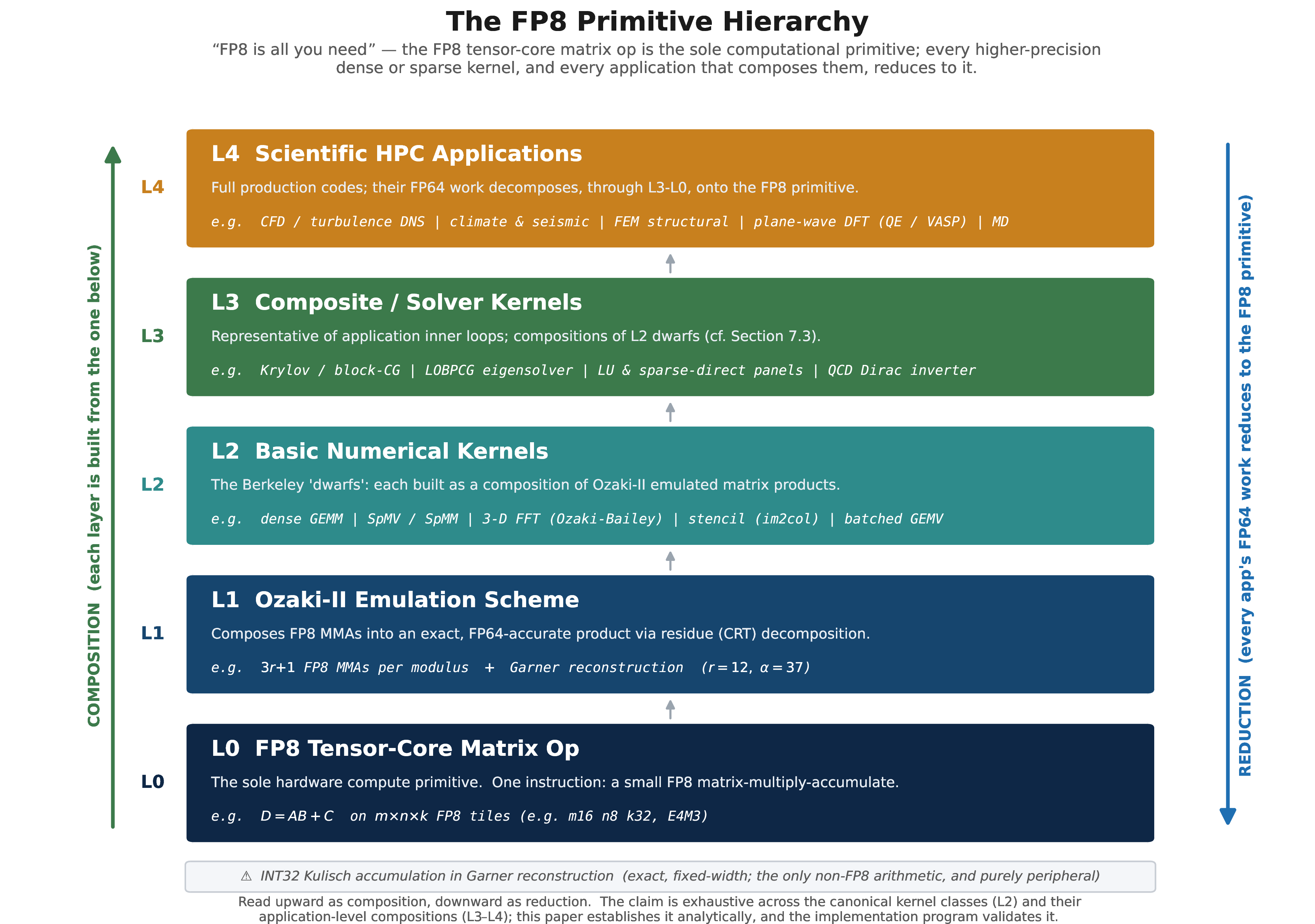
The hierarchy has five layers. At the bottom, L0 is the sole hardware primitive: a single FP8 matrix-multiply-accumulate \(D = AB + C\) on small tiles (e.g.\(m16\,n8\,k32\), E4M3). Directly above it, L1 is the Ozaki II scheme, which composes \(3r{+}1\) FP8 MMAs per modulus, followed by Garner reconstruction, into an exact fp64-accurate matrix product (§2). L2 is the set of basic numerical kernels—the dwarfs themselves: dense GEMM, SpMV and SpMM, the three-dimensional FFT, structured stencils, batched GEMV—each realised as a composition of L1 emulated products. L3 is the layer of composite and solver kernels that constitute the inner loops of real applications—Krylov and block-CG iterations, LOBPCG eigensolvers, dense and sparse-direct factorisation panels, the lattice-QCD Dirac inverter—each a composition of L2 dwarfs; §7 substantiates this layer directly. Finally, L4 is the full scientific application—computational fluid dynamics and turbulence DNS, climate and seismic codes, finite-element structural analysis, plane-wave density-functional theory, molecular dynamics—whose fp64 work decomposes, through L3 and L2 and L1, onto the L0 primitive.
The picture is the thesis, and its force comes from the exhaustiveness the dwarfs already established. Their taxonomy spans scientific computing by construction; if every dwarf (L2) reduces to the FP8 primitive through Ozaki II, then by composition every L3 kernel and every L4 application reduces to it as well. We are not claiming to have inspected every code in existence—we are observing that the dwarfs did the spanning, and closing the reduction from the dwarfs down to a single operation one layer below them. In the conventional view, L2 would rest on a hardware fp64 multiplier; the contribution of this paper is to show that it rests instead on the FP8 tensor-core op, with fp64 demoted from a hardware primitive to a derived guarantee. We believe such a top-down, primitive-level treatment has been conspicuously absent from recent debates about reduced precision and AI–HPC convergence, which tend to begin and end at the level of individual kernels or individual architectures.
This is a falsifiable claim, not a slogan, and the Tensor–Memory Equilibrium model of §4 is the instrument built to test it. The claim is operational: every dwarf, and every composition of dwarfs, must stay on the bandwidth-bound side of the roofline (or remain otherwise fp64-competitive) when built on FP8 Ozaki II. That is a statement about performance characteristics—operational intensity, the emulated compute ceiling \(P_{\mathrm{\small fp8}}/\alpha\), the bandwidth multiplier \(\beta\), the reconstruction cost \(\gamma\)—and a performance model is exactly the right tool to confirm or refute it, provided it captures those quantities. Were the model to show any canonical kernel driven compute-bound on the FP8 ceiling, or any composition forced persistently past the memory-bound threshold with no architectural escape, or any kernel demanding a primitive that is neither an FP8 matrix op nor the peripheral INT32 reduction, the thesis would be false and the model would say so. That it instead returns a positive verdict across the dwarfs is the analytical content of this paper. We are explicit about the division of labour: this paper performs the analysis that establishes the claim; a follow-on implementation effort validates it on production silicon by realising the L1–L2 kernels and measuring delivered performance end-to-end (§8.3). The questions that this structural claim leaves genuinely open—chiefly the efficiency with which each reduction is realised, captured by \(\beta\) under composition—are second-stage matters of architecture and engineering layered on top of the bound, and we treat them as such, concentrating them in §9 rather than threading caution through the analysis.
1.1.0.1 Roadmap.
§2 reviews the two Ozaki schemes (the L1 layer) and related FP64-emulation work. §3 establishes the architectural baselines. §4 develops the TME performance model. §5 gives the design of the basic memory-bound kernels (L2). §6 reports the projections. §7 substantiates the composite/solver layer (L3), showing that the kernels representative of real applications reduce to the same primitive. §8 discusses the broader landscape and implications, and §9 states the conditions under which the thesis would be falsified and confronts the principal objections to it. §10 concludes. Appendices contain the error-analysis sketch, corrected pseudocode, Garner’s derivation, and a detailed analysis of the sparse primitive establishing that the bandwidth multiplier remains near unity for sparse kernels (Appendix 16).
2 Background and Related Work↩︎
We summarise the two Ozaki schemes at the level of detail required for the performance model. Readers familiar with [13], [16] can skim this section.
2.1 Error-Free Transformations and the Ozaki Scheme↩︎
Let \(a,b\in\mathbb{F}\) be working-precision floats. Veltkamp/Dekker splitting expresses \(a=a_h+a_\ell\) with \(a_h\) holding the leading bits and \(a_\ell\) the trailing bits, all in \(\mathbb{F}\); the product \(ab\) then equals \(a_h b_h + a_h b_\ell + a_\ell b_h + a_\ell b_\ell\), computed exactly when each factor fits in \(\mathbb{F}\). The Ozaki scheme [13] generalises this idea to dense matrices, replacing two-word splitting by \(s\)-way slicing along the inner-product direction.
2.2 Ozaki Scheme I: Mantissa Slicing↩︎
Given \(A\in\mathbb{F}^{m\times k}\) and \(B\in\mathbb{F}^{k\times n}\), Ozaki I forms decompositions \[A=\sum_{p=1}^{S_A}A^{(p)},\qquad B=\sum_{q=1}^{S_B}B^{(q)}, \label{eq:ozaki1-decomp}\tag{1}\] in which each \(A^{(p)}\) and \(B^{(q)}\) has a bounded mantissa width compatible with the target tensor format. The reconstruction is \[C \;\approx\;\sum_{p=1}^{S_A}\sum_{q=1}^{S_B} A^{(p)}B^{(q)}, \label{eq:ozaki1-recon}\tag{2}\] summed in working precision, at dominant cost \(S_A\!\cdot\!S_B\) low-precision GEMMs.
2.2.0.1 Substrate-specific scaling.
The three candidate tensor-core substrates—fp16, int8, and fp8—differ in how 1 –2 is actually computed.
fp16 tensor cores. Each \(A^{(p)}\) and \(B^{(q)}\) is stored directly as an fp16 matrix, and the tensor-core MMA accumulates \(A^{(p)}B^{(q)}\) in fp32. No additional integer scaling is required.
int8 tensor cores. Each slice carries a floating-point mantissa range, but the int8 engine consumes signed integers. The decomposition therefore associates each slice with a per-slice power-of-two exponent: \(A^{(p)} = 2^{e_p}\!\cdot\!\widetilde{A}^{(p)}\) and \(B^{(q)} = 2^{f_q}\!\cdot\!\widetilde{B}^{(q)}\), where \(\widetilde{A}^{(p)},\widetilde{B}^{(q)}\!\in\!\mathbb{Z}^{8}\) are the signed-integer mantissa slices fed to the int8 engine, and the reconstruction accumulates \(2^{e_p+f_q}\!\cdot\!(\widetilde{A}^{(p)} \widetilde{B}^{(q)})\) in fp64 [14], [15]. The integer products themselves are computed exactly in int32.
fp8 tensor cores. fp8 (E4M3) consumes only a 3+1-bit mantissa per element, so the slicing of an fp64 mantissa requires more slices than the int8 case; in addition, the fp8 engine accumulates in fp32 rather than int32, and a separate quantisation correction is required to handle the implicit normalisation of the fp8 format. The corresponding scheme is described in detail in [21] and is the basis of the FP8 variant of Ozaki II that we discuss in §2.4.
2.2.0.2 Slice counts: accumulator-bound analysis.
The required slice count is governed jointly by the input mantissa width and by the accumulator precision. For fp64-accurate output with summation length \(k\), the requirement that the accumulator hold the sum of \(k\) products of \(b\)-bit slices exactly is \[2b + \lceil \log_2 k \rceil \;\leq\; w_{\text{acc}}, \label{eq:slice-bits}\tag{3}\] where \(w_{\text{acc}}\) is the number of significand bits available in the accumulator (24 for fp32, 31 for int32 signed). Inverting 3 gives the maximum safe payload \(b^\star\!=\!(w_{\text{acc}} \!-\!\lceil\log_2 k\rceil)/2\) bits per slice. The slice count needed to cover the 53-bit fp64 mantissa is then \(S\!\approx\!\lceil 53/b^\star \rceil\).
Table 1 reports the resulting slice counts for representative inner-dimension lengths \(k\). Three observations follow.
| Substrate | \(w_{\text{acc}}\) | \(k\!=\!256\) | \(k\!=\!1024\) | \(k\!=\!4096\) | \(k\!=\!16384\) |
|---|---|---|---|---|---|
| / -accum | 24 | \(\approx 4\) | \(\approx 5\) | \(\approx 6\) | \(\approx 8\) |
| / -accum | 31 | \(\approx 5\) | \(\approx 6\) | \(\approx 7\) | \(\approx 8\) |
| / -accum | 24 | \(\approx 12\) | \(\approx 14\) | \(\approx 18\) | — |
6pt
Reported empirical values: : \(S\!\approx\!3\)–\(4\) at moderate \(k\) [14]; : \(S\!\approx\!7\)–\(10\) at \(k\!\leq\!16384\) [14], [15]; : \(S\!\geq\!11\) in the configurations of [21]. Empirical values exceed the accumulator-bound minimum because of input distributional effects (loss of leading bits when the entries’ magnitudes vary substantially across the inner-product
summation).
For fp16 tensor cores with fp32 accumulation, the bound is tight: at \(k\!=\!4096\), only about 6 bits per slice can be safely accumulated, even though fp16 can carry 11. In other words, at large \(k\), the fp16/fp32 substrate is accumulator-bound rather than input-bound, and the slice count grows accordingly.
For int8 cores with int32 accumulation, the bound is loose: at \(k\!=\!4096\), the safe payload is 9.5 bits, which exceeds the 7-bit int8 input. Consequently, the slice count is governed by the input mantissa, not by the accumulator, and grows only logarithmically with \(k\). At large \(k\), the int8 substrate therefore requires comparable or fewer slices than fp16, contrary to a naive ordering by input precision.
For fp8 tensor cores, the small input mantissa (effectively 4 bits) combined with the fp32 accumulator constraint produces the highest slice count of the three; Mukunoki’s reported \(S\!\geq\!11\) for FP8 [21] is consistent with Table 1.
2.2.0.3 Quadratic scaling.
The total number of low-precision GEMMs scales as \(\Theta(S^2)\), which is the dominant disadvantage of Ozaki I for bandwidth-limited problems: even with fused decomposition, the temporal volume of arithmetic grows quadratically in the slice count. This is the principal motivation for the linearly-scaling Ozaki II scheme described next.
2.3 Ozaki Scheme II: Modular Arithmetic via the CRT↩︎
The Chinese Remainder Theorem-based Ozaki II scheme, proposed by Ozaki, Uchino and Imamura in 2025 [16], replaces the slice decomposition by a residue decomposition over a set of pairwise-coprime moduli. The algorithm consists of three phases.
2.3.0.1 Phase 1: Integer scaling.
Diagonal scaling matrices \(D\!\in\!\mathbb{F}^{m\times m}\) and \(E\!\in\!\mathbb{F}^{n\times n}\), chosen with power-of-two diagonals to be exactly invertible in fp64, are used to form \[\tilde{A} = \lfloor DA\rceil\in\mathbb{Z}^{m\times k},\qquad \tilde{B} = \lfloor BE\rceil\in\mathbb{Z}^{k\times n}, \label{eq:scale}\tag{4}\] where the rounding \(\lfloor\,\cdot\,\rceil\) is to nearest integer. The integer matrices \(\tilde{A},\tilde{B}\) have magnitudes bounded by the chosen scaling factor, typically \(2^{p-1}-1\) for a representation width of \(p\) bits.
2.3.0.2 Phase 2: Modular GEMMs.
Choose pairwise-coprime moduli \(m_1<m_2<\cdots<m_r\) large enough that \[M = \prod_{i=1}^r m_i \;>\; 2\cdot \max_{ij}\bigl|(\tilde{A}\tilde{B})_{ij}\bigr|, \label{eq:M-bound}\tag{5}\] which guarantees that the integer product can be uniquely reconstructed from its residues. For each \(i\in\{1,\dots,r\}\) compute \[C^{(i)} \;=\; \bigl(\tilde{A} \bmod m_i\bigr)\;\bigl(\tilde{B} \bmod m_i\bigr) \bmod m_i. \label{eq:modgemm}\tag{6}\] On int8 tensor cores each \((\tilde{A}\bmod m_i)\cdot(\tilde{B}\bmod m_i)\) is a standard int8 GEMM accumulated in int32. When using fp8 tensor cores the modular reduction must be carried out in scaled floating point following the technique of [20].
2.3.0.3 Phase 3: CRT reconstruction (Garner’s algorithm).
We apply Garner’s algorithm [28], [29] to recover the integer product element-wise. Writing \(C_{ij}=v_1+v_2 m_1+v_3 m_1m_2+\cdots\) in mixed radix, the digits \(v_k\) are computed iteratively as \[\begin{align} v_1 &= C^{(1)}_{ij},\\ v_k &= \biggl(C^{(k)}_{ij}-\sum_{j=1}^{k-1}v_j\prod_{\ell=1}^{j-1}m_\ell\biggr) \cdot\biggl(\prod_{\ell=1}^{k-1}m_\ell\biggr)^{-1} \pmod{m_k}, \quad k\ge 2. \end{align} \label{eq:garner}\tag{7}\] The modular inverses \(\bigl(\prod_\ell m_\ell\bigr)^{-1}\pmod{m_k}\) are precomputed once. The recovered integer is finally rescaled back to floating point via \(C \approx D^{-1}\tilde{C} E^{-1}/(\sigma_A\sigma_B)\), where \(\sigma_A,\sigma_B\) are the scalar magnitudes hidden inside \(D,E\).
2.3.0.4 Linear scaling.
The cost is \(r\) low-precision GEMMs plus the \(O(r^2)\) element-wise reconstruction. Critically, \(r\) scales linearly in the required exponent range for FP64-equivalent dynamic range; published parameter sets use \(r\!\in\![13,16]\) on int8 cores [16] and \(r\!\in\![8,12]\) on fp8 cores [20], with the exact value driven by the desired error guarantee.
2.4 The fp8 Variant of Ozaki II↩︎
Uchino, Ozaki and Imamura observed in early 2026 that the original Ozaki II algorithm cannot be directly adapted to fp8 matrix-multiply-accumulate units, because modular reduction is fundamentally an integer operation [20]. They introduced a quantisation trick that emulates modular arithmetic over fp8 by exploiting the fact that an fp8 (E4M3) value can represent integers up to \(\pm 448\) exactly. This adaptation is the reason that Ozaki II remains viable on Blackwell Ultra and on the upcoming NVIDIA Rubin GPU, both of which significantly downgrade int8 in favour of fp8/fp4 [20], [21].
This paper assumes the existence of this fp8 adaptation but does not re-derive it. Our TME model is parameterised so that the choice of underlying tensor format simply rescales the compute multiplier \(\alpha\) and the reconstruction latency \(\gamma\), without altering the model’s structure.
2.4.0.1 Moduli count and the \((3r+1)\) FP8 cost structure.
The performance projections in later sections adopt \(r\!=\!12\) moduli for the fp8 Ozaki II variant, the value recommended by Mukunoki [21] (who report \(r\!\in\![11,14]\) for fp64-equivalent accuracy on the fp8 (E4M3) substrate), together with the full \((3r{+}1)\) fp8 op count. The latter, clarified by Imamura (private communication and [2]), reflects that each fp64-equivalent residue product on the FP8 substrate expands into \((3r{+}1)\) FP8 MMAs rather than \(r\), because the Karatsuba structure used internally to emulate signed int9 on FP8 introduces a factor-of-three multiplier on the residue planes (the trailing \(+1\) being the max-magnitude estimation pass). For the INT8 substrate the count is \((s+1)\) where \(s\) is the slice count, \(\sim\!2.5\times\) cheaper per modulus but requiring more moduli. Thus the fp8 compute multiplier is \(\alpha=3r{+}1=37\) at \(r\!=\!12\), and all dense compute-bound ceilings in §4–§3 use this value (an earlier draft used the moduli-only count \(\alpha=r\), which overstated the fp8 compute ceiling by \(\approx\!3\times\); we thank the NVIDIA libraries/DevTech team for flagging this). Crucially, the correction is confined to the compute-bound regime: it scales the dense ceiling by \(r/(3r{+}1)\) but leaves the parity-row structure of Table 3 and the H100-relative scaling of Table 4 unchanged, because those rows are governed by HBM-bandwidth ratios, not by the compute-ceiling constant. This is the analytic content of the dense-vs-memory-bound distinction we make explicit in Case C of §4.
2.5 Error Analysis↩︎
Both Ozaki I and Ozaki II provide provable error bounds for the emulated product, in contrast to ad-hoc mixed-precision schemes. For Ozaki II with \(r\) moduli chosen by the criterion 5 , the worst-case componentwise relative error is bounded by the working-precision unit round-off \(u_{\mathrm{\small fp64}}\approx 2^{-53}\) plus the floating-to-integer rounding introduced in 4 [22]. In practice, for inputs with bounded condition number, the observed relative error is within \(2\)–\(10\,u_{\mathrm{\small fp64}}\) [16]; this behaviour was confirmed in the recent ADP work of Schwarz et al. [23], who report less than 10% overhead for componentwise-accurate DGEMM emulation on Blackwell.
We refer the reader to [22] for the full componentwise analysis; the practical implication for this paper is that the kernels we discuss inherit the same error bound as the underlying emulated GEMM, modulo the trivial summation rounding incurred at the reconstruction step.
2.5.0.1 Dynamic range and the choice of \(r\) are not free, but they are bounded and automatable.
A fair objection to any fixed-slice emulation is that integer/fixed-point residue arithmetic carries no exponent, so the safe number of moduli \(r\) depends on the dynamic range of the specific operands and cannot be assumed constant: a single optimistic \(r\) may under-serve ill-conditioned inputs, and determining the right \(r\) per operation is itself work that must be charged. We make two points. First, the value used throughout this paper, \(r=12\), is the fp64-equivalent setting recommended by Mukunoki [21] (\(r\!\in\![11,14]\)) rather than a throughput-maximising guess; the projections should be read as a function of \(r\) (each unit of \(r\) scaling the dense compute ceiling by \(\approx r/(3r{+}1)\)), with the larger end of the range the conservative choice for guaranteed accuracy. Second, the per-input selection of \(r\) need not be hand-tuned or expensive: the Exponent-Span-Capacity (ESC) estimator and Automatic Dynamic Precision (ADP) framework of Schwarz et al. [23] choose the slice count per GEMM at runtime, fully GPU-resident, with automatic fallback to native fp64, and report less than \(10\%\) overhead even under worst-case configurations, validated against adversarial BLAS-grading tests. The TME model accommodates this directly by letting \(\alpha=(3r{+}1)\) track an ESC-chosen \(r\) rather than a fixed constant (§8.3 and the per-row treatment of Appendix 14). The residual question—how often ADP must fall back on real scientific inputs, and whether that fallback materially erodes the memory-roof advantage—is genuinely empirical and is one of the measurements we prioritise in §8.3; notably, on B300 the fallback target is the small surviving native fp64 pipe, not a zero-fp64 part, so an occasional fallback degrades gracefully rather than catastrophically.
2.6 Other FP64 Emulation Approaches↩︎
Several alternative paths exist for emulating high-precision arithmetic on low-precision tensor units. Markidis et al. [30] explored fp16 tensor cores for fp32-equivalent accuracy, the natural ancestor of all modern emulation work. Iterative-refinement solvers [31], [32] use low-precision GEMMs as inner kernels and correct residuals in high precision, achieving high accuracy on solvers but not on bare GEMM-like primitives. More recently, MixPert and similar adaptive-precision frameworks compose low-precision tensor operations with correction terms.
Ozaki-style emulation is distinctive in that it provides provable componentwise error guarantees on the bare matrix product itself, without requiring an outer iteration or a problem-specific tuning loop. This property is essential for drop-in replacement of cuBLAS DGEMM in scientific codes, which is exactly the use case NVIDIA targeted with the October 2025 cuBLAS integration [17].
2.7 Tensor Cores for Memory-Bound Kernels: Prior Art↩︎
There is a parallel literature, largely independent of Ozaki, on making memory-bound kernels use tensor cores at all—irrespective of precision considerations. TCStencil [33], SPTCStencil [34] and SparStencil [35] reformulate stencil sweeps as block-sparse GEMMs amenable to dense or sparse tensor cores. These works treat the precision question orthogonally (typically retaining fp32 or fp16). Our contribution sits at the intersection of the two threads: we want both (i) the tensor-core mapping that the stencil community has developed, and (ii) the fp64-accurate emulation that the Ozaki community has developed. The TME model is the analytic tool that lets us reason about both simultaneously.
Finally, the present work sits within a broader, ongoing reassessment of the relationship between AI-oriented hardware and scientific computing, of which recent strategic surveys of how HPC must adapt to AI-era silicon [36] are representative. That literature documents the shift—native fp64 ceasing to be the assumed foundation of HPC—and its consequences for the field; our aim is complementary and more specific, namely to supply the primitive-level theory that shows the shift is not merely survivable but sound, with the FP8 matrix op as the foundation onto which the established kernel taxonomy maps.
3 Architectural Analysis: The FP64 Cliff↩︎
We now establish the architectural baselines used throughout the rest of the paper. All numbers in Table 2 are taken from the official NVIDIA datasheets and corroborated by independent microbenchmarks [3]–[6]. We report dense throughput per single GPU unless explicitly marked as sparse, because real HPC workloads do not generally exhibit the 2:4 structured sparsity required to reach the sparse rates.
| Metric | H100 | B200 | B300 | R200 |
| (Hopper) | (Blackwell) | (Blackwell Ultra) | (Rubin) | |
| FP64 Vector (TFLOPS) | 34 | 40 | \(\sim\)1.3 | \(\sim\)33 |
| FP64 Tensor, native (TFLOPS) | 67 | 40 | \(\sim\)1.2 | —* |
| FP64 Matrix, emulated (TFLOPS) | — | — | via Ozaki II | \(\sim\)200 |
| FP16/BF16 Tensor (TFLOPS, dense) | 989 | 2,250 | 2,500 | — |
| TF32 Tensor (TFLOPS, dense) | 494 | 1,100 | 1,250 | 2,000 |
| FP8 Tensor (TFLOPS, dense) | 1,979 | 4,500 | 5,000 | \(\sim\)4,000 |
| FP6 Tensor (TFLOPS, dense) | — | — | — | 17,500 |
| INT8 Tensor (TOPS, dense) | 1,979 | \(\sim\)155 | \(\sim\)165 | \(\sim\)250 |
| FP4 / NVFP4 (TFLOPS, dense) | — | 7,000 | 10,000 | 35,000 |
| HBM Bandwidth (TB/s) | 3.35 | 7.7–8.0 | 8.0 | 22 |
| HBM Capacity (GB) | 80 | 180–192 | 279–288 | 288 |
| FP8 : native FP64 ratio | 30:1 | 113:1 | 3800:1 | 120:1\(\dagger\) |
| Memory ridge /B (native) | 10.1 | 5.0 | 0.16 | 1.5 |
4pt
* Rubin specifications list FP64 matrix performance under an explicit “Emulated DGEMM” column rather than as a native tensor-core rate [9], [10]. \(\dagger\) FP8 to native vector FP64; the FP8 : emulated-DGEMM ratio is \(\sim\!37{:}1\) at the corrected \(\alpha=3r{+}1\) (\(r{=}12\)).
3.0.0.1 Reading the table.
Four columns—H100, B200, B300, and R200—trace a clear architectural trajectory. Native fp64 compute is no longer growing with each generation; on B300 it has effectively been removed, and on Rubin NVIDIA has chosen to expose “Emulated DGEMM” as an explicit, first-class column in the official specifications [9]. At the same time, the low-precision matrix pipes (fp8, NVFP4) and the HBM bandwidth have each grown by factors of \(2\)–\(3\) per generation, with Rubin’s \(22\) TB/s HBM4 marking a \(2.75\times\) jump over B300. Any performance model for scientific computing on these architectures must therefore treat emulation not as an optimisation but as the native execution model for fp64 matrix operations.
3.0.0.2 Why Ozaki II runs through fp8 on these architectures.
The int8 rate on Blackwell Ultra and Rubin has not scaled with fp8 or NVFP4—in fact it has decreased relative to Hopper, as silicon area has been redirected toward low-precision floating-point matrix units. The natural path to high emulation performance on these architectures therefore runs through fp8 [20], [21]. On fp8 the B300 delivers \(5\) PFLOPS dense and \(10\) PFLOPS sparse; with \(r\!=\!12\) moduli and the full \((3r{+}1)\) fp8 cost (\(\alpha=37\)), the effective upper bound on emulated fp64 throughput is \(5{,}000/37 \approx 135\) TFLOPS dense. On Rubin, \(4\) PFLOPS dense fp8 with the same parameters yields \(\approx 108\) TFLOPS; NVIDIA’s published \(\sim 200\) TFLOPS “Emulated DGEMM” figure exceeds this dense-fp8\(/(3r{+}1)\) bound and presumably reflects a different substrate (e.g., INT8, at \((s{+}1)\) per modulus) or modulus choice [22], [23].
3.0.0.3 Where the native memory ridge sits.
Combining the native fp64 compute roof with HBM bandwidth gives ridge points of \(10.1\) FLOPS/B on H100, \(5.0\) FLOPS/B on B200, \(0.16\) FLOPS/B on B300, and \(1.5\) FLOPS/B on Rubin. These four numbers tell three distinct stories. On H100 and B200, the ridge sits above the operational intensity of every standard memory-bound primitive (SpMV \(\sim 0.2\), stencils \(\sim 0.5\), batched GEMV \(\sim 1\)–\(4\)), so those kernels are bandwidth-bound natively and the architecture is balanced for the workload class. On B300, the ridge has collapsed to \(0.16\) FLOPS/B, below the operational intensity of every standard scientific kernel; the native pipe is the bottleneck even for SpMV. On Rubin, the picture is genuinely mixed: the bandwidth jump to \(22\) TB/s combined with the modest \(33\) TFLOPS vector fp64 pushes the ridge to \(1.5\) FLOPS/B, which puts SpMV (\(\sim 0.2\)) and stencils (\(\sim 0.5\)) back into the memory-bound regime where native fp64 vector is once again usable, while batched GEMV and dense GEMM sit at or above the ridge and benefit from the Emulated DGEMM path. In other words, Rubin partially restores the native-fp64-viable regime for the lowest-OI kernels, and Ozaki II picks up the rest.
4 The Tensor–Memory Equilibrium Model↩︎
We now develop the analytic performance model used in the rest of the paper. Let a kernel perform \(W\) fp64-equivalent floating-point operations on \(Q\) bytes of memory traffic, so that its operational intensity is \(\mathrm{OI}=W/Q\). We adopt OI in preference to “operational intensity” to avoid notational collision with AI throughout this paper.
4.1 Native FP64↩︎
The Roofline model [1] predicts the native execution time as \[T_{\text{nat}} \;=\; \max\!\left(\frac{W}{P_{\mathrm{\small fp64}}},\frac{Q}{B_\text{mem}}\right) \;+\; L_{\text{mem}}, \label{eq:tnat}\tag{8}\] where \(P_{\mathrm{\small fp64}}\) is the peak fp64 throughput, \(B_\text{mem}\) the HBM bandwidth and \(L_\text{mem}\) the cold-start latency (assumed amortised for the workload sizes considered). The kernel is memory-bound when \(I<P_{\mathrm{\small fp64}}/B_\text{mem}\), compute-bound otherwise.
4.2 Emulated Execution↩︎
Replacing native fp64 by Ozaki II introduces three overhead parameters.
Definition 1 (Emulation parameters). For a fixed Ozaki II configuration on a given hardware target,
\(\;=\;\) number of low-precision tensor-core MMAs required per fp64 fused multiply–add. For Ozaki II this is essentially \(r\) (the number of moduli), modulo constant overhead from index arithmetic.
\(\;\ge 1\;\) is the bandwidth multiplier: the ratio of bytes moved by the emulated kernel to the bytes that the equivalent native fp64 kernel would move. \(\beta=1\) for fully fused on-chip decomposition (residues live in registers and never touch global memory); \(\beta=r\) in the unfused regime (each residue plane is materialised in HBM).
\(\;\ge 0\;\) is the per-output reconstruction latency, in seconds per output element, capturing the cost of Garner’s algorithm.
The emulated time is then \[T_{\text{emu}} \;=\; \max\!\left(\frac{\alpha\, W}{P_{\text{low}}},\frac{\beta\, Q}{B_\text{mem}}\right) \;+\; \gamma\, n_\text{out}, \label{eq:temu}\tag{9}\] where \(P_{\text{low}}\) is the relevant low-precision tensor throughput (\(P_{\mathrm{\small fp8}}\), \(P_{\mathrm{\small int8}}\), etc.) and \(n_\text{out}\) is the number of output elements.
4.3 Crossover Analysis↩︎
Let \(\rho \;=\; P_{\text{low}}/P_{\mathrm{\small fp64}}\) be the precision ratio (e.g., \(\rho\approx 3800\) for fp8 on B300). The compute multiplier \(\alpha\) is the number of low-precision MMAs per high-precision op. On the fp8 substrate this is \(\alpha=(3r{+}1)\): each of the \(r\) residue planes expands into three fp8 MMAs (the Karatsuba structure used to emulate signed int9), plus one MMA for the max-magnitude estimation pass. At the recommended \(r\!=\!12\) this gives \(\alpha=37\). (On the INT8 substrate the cost is \((s{+}1)\) with \(s\) the slice count—\(\sim\!2.5\times\) cheaper per modulus, but requiring more moduli; see §3.)
4.3.0.1 Case A: Native compute-bound, emulation memory-bound.
This is the regime that the B300 collapses into for nearly every standard kernel. Equations 8 and 9 give \[T_{\text{nat}} = \frac{W}{P_{\mathrm{\small fp64}}},\qquad T_{\text{emu}} = \frac{\beta Q}{B_\text{mem}}+\gamma n_\text{out},\] and the emulation is profitable when \[\frac{W}{P_{\mathrm{\small fp64}}} \;>\; \frac{\beta Q}{B_\text{mem}} + \gamma n_\text{out}. \label{eq:case-a-condition}\tag{10}\] Ignoring \(\gamma\) momentarily, and assuming \(\beta=1\) (the fused case), the speedup of emulation over native is \[\frac{T_\text{nat}}{T_\text{emu}} \;=\;\frac{W/P_{\mathrm{\small fp64}}}{Q/B_\text{mem}} \;=\;\frac{I\cdot B_\text{mem}}{P_{\mathrm{\small fp64}}}, \label{eq:case-a-speedup}\tag{11}\] that is, the speedup equals the kernel’s distance into the compute-bound region of the native roofline. On the B300 with \(I=0.5\) (a 7-point stencil), \(B_\text{mem}=8\) TB/s, \(P_{\mathrm{\small fp64}}=1.3\) TFLOPS, this gives a speed-up of \(0.5\cdot 8/1.3 \approx 3.1\times\).
4.3.0.2 Case B: Both regimes memory-bound (small \(I\)).
When the native kernel is already memory-bound, emulation cannot improve time-to-solution beyond \(T_\text{nat}\) in the best case (\(\beta=1\)). More precisely, \(T_{\text{emu}}/T_{\text{nat}}\to\beta\). Hence fused decomposition (\(\beta=1\)) yields parity, and unfused decomposition is strictly worse. This gives the important practical guidance: for genuinely memory-bound kernels in the small-\(I\) regime, register-level fusion is not just an optimisation; it is a correctness requirement for emulation to be viable at all.
4.3.0.3 Case C: Both regimes compute-bound (dense GEMM).
Here the speedup is \(\rho/\alpha\), and the bandwidth roof is irrelevant. On the B300 with fp8 cores at \(r\!=\!12\) (\(\alpha=3r{+}1=37\)), this gives a throughput ceiling of \(5{,}000/37 \approx 135\) TFLOPS, which is \(\approx 104\times\) over B300 native fp64 (\(1.3\) TFLOPS). This is the regime in which Ozaki II for dense GEMM has been most extensively studied [20], [21], [23]. Note that the \((3r{+}1)\) fp8 cost structure bites only in this compute-bound case, where the kernel runs at the emulation ceiling and the throughput scales as \(1/\alpha\). In Cases A and B the kernel is bandwidth-limited and never reaches the compute ceiling, so the same factor merely lowers the emulation ridge—the operational intensity below which a kernel stays memory-bound—from \(P_{\mathrm{\small fp8}}/(rB_\text{mem})\) to \(P_{\mathrm{\small fp8}}/((3r{+}1)B_\text{mem})\); on B300 this is a shift from \(\approx 52\) to \(\approx 17\) FLOPS/B, still far above the intensity of every memory-bound kernel surveyed (§6).
4.4 The TME Picture↩︎
Figure 2 draws the TME roofline for both B300 and Rubin. The native fp64 roof on B300 is flat at \(1.3\) TFLOPS, and on Rubin at \(\sim 33\) TFLOPS for vector fp64. Ozaki II with fused decomposition follows the memory roof up to its own compute ceiling: \(\approx 135\) TFLOPS on B300 (dense fp8 at \(5\) PFLOPS, \(r{=}12\), \(\alpha=3r{+}1=37\)) and \(\approx 108\) TFLOPS on Rubin (dense fp8 at \(4\) PFLOPS with the same parameters). We note in passing that Rubin’s dense-fp8 throughput is actually slightly lower than B300’s—NVIDIA has reallocated silicon area from fp8 to NVFP4/fp6 on Rubin, so the dense-fp8 Ozaki II ceiling is essentially flat between B300 and Rubin. What changes generationally is the memory roof, which jumps from \(8\) TB/s to \(22\) TB/s, lifting the achieved throughput across the entire bandwidth-bound region. NVIDIA’s conservative published Emulated-DGEMM figure for Rubin (\(\sim 200\) TFLOPS) corresponds to a parameter set with more moduli or with margin reserved for componentwise-error guarantees [22], [23].
Two observations follow directly from the figure and are the central quantitative message of this paper.
4.4.0.1 Memory-bound regime: parity with the memory roof.
In the bandwidth-bound region (left of the ridge point) the Ozaki II/fp8 curve overlaps the memory roof exactly. This is precisely what scientific computing requires: whatever bandwidth the architecture provides, the emulated path can consume. On B300 this lifts memory-bound kernels from the collapsed \(1.3\) TFLOPS native floor up to the \(8 I\) TFLOPS memory roof—a gain that ranges from \(1.2\times\) at SpMV-grade intensities (\(I\!\approx\!0.2\)) to \(9.2\times\) at batched-GEMV intensities (\(I\!\approx\!1.5\)). On Rubin, the same emulated curve follows a \(22 I\) TFLOPS memory roof, \(2.75\times\) higher in absolute throughput than B300 across the entire memory-bound region. This bandwidth-driven gain is the dominant Rubin advantage and is felt by every HPC kernel with \(I \lesssim P_{\mathrm{\small fp8}}/((3r{+}1)\cdot B_{\text{mem}}) \approx 17\) FLOPS/B (the corrected emulation ridge on B300 at \(r{=}12\); an earlier draft placed this at \(\approx 62\) using \(\alpha=r\)).
4.4.0.2 Compute-bound regime: surpassing B200 by a wide margin.
In the compute-bound region (right of the ridge point) the Ozaki II/fp8 curve saturates at \(\sim 135\) TFLOPS on B300 and \(\sim 108\) TFLOPS on Rubin (dense fp8\(/(3r{+}1)\) at \(r{=}12\)). For reference, B200’s native fp64 ceiling sits at \(40\) TFLOPS—so the emulated path on B300 exceeds B200 by \(\approx 3.4\times\) and on Rubin by \(\approx 2.7\times\), in the regime where native fp64 on B200 was previously the gold standard. In other words, the TME roofline shows that emulation does not merely compensate for the fp64 collapse; it carries the entire operational-intensity spectrum above the best native fp64 performance offered on the prior generation, even after the full \((3r{+}1)\) fp8 cost is charged. This is the quantitative argument for treating Ozaki II as the new baseline rather than as a fallback.
![Figure 2: TME roofline projection for B300 and Rubin. Each platform hasits own memory roof (black for B300, dotted violet for Rubin) and itsown native fp64 ceiling (red for B300, dashed violet for Rubinvector; B200 in dashed orange for reference). The Ozaki II/fp8curves (blue for B300, teal for Rubin) trace the memory roof in thebandwidth-bound regime and saturate at the emulation compute ceiling inthe compute-bound regime. The Ozaki II/FP8 ceiling is \approx135 TFLOPS on B300 and \approx 108 TFLOPS on Rubin (each = P_{\mathrm{\small fp8}}/(3r{+}1)with r=12, \alpha=37); NVIDIA’s conservative published “Emulated DGEMM” figurefor Rubin is \sim 200 TFLOPS [9], [10],which the model meets at a coarser parameter set (the published figureexceeds the dense-fp8/(3r{+}1) bound and presumably reflects adifferent substrate or modulus choice).Across the entire intensity spectrum, the emulated curves dominate theB200 native fp64 reference line.](/article/2606.06510/_pdflatex/pfrvqgdu.png "fig:")
5 Implementation Strategies for Memory-Bound Kernels↩︎
The crossover analysis of §4 establishes that the kernel design discipline—and specifically the value of \(\beta\)—is what determines whether Ozaki II is profitable on memory-bound workloads. We now describe how to drive \(\beta\to 1\) for the three canonical bandwidth-limited primitives.
5.1 Register-Level Fusion: the Common Pattern↩︎
The unifying technique is to perform the decomposition (4 and the residue reduction \(\bmod\,m_i\)) after the working-precision operand has arrived in registers, and to perform the reconstruction (7 ) on the accumulator before the result is stored. This keeps the residue planes off the HBM bus. In CUDA terms:
Each thread block reads a tile of \(A\) (and possibly \(B\)) in fp64 from HBM into shared memory.
Within the tile, each warp computes the \(r\) residue planes in registers, using a small precomputed table of moduli stored in
constantmemory.The warp issues \(r\) low-precision
wmma::mma_sync(or equivalenttcgen05) instructions, each operating on the \(i\)th residue plane.After the tile loop, the warp reconstructs the integer accumulator via Garner’s algorithm 7 , rescales by \(D^{-1}E^{-1}\), and stores one fp64 result.
Because the residue planes never reach HBM, the bandwidth multiplier \(\beta\) equals 1 (modulo a negligible constant for the moduli table and the precomputed Garner inverses). The compute multiplier \(\alpha\) equals \(3r{+}1\) on the fp8 substrate (the three Karatsuba fp8 MMAs per modulus plus the max-magnitude pass; \(\alpha=r\) would hold only if a single MMA per modulus sufficed, as on an INT8 substrate with \(s{+}1\) slices). The reconstruction latency \(\gamma\) is \(O(r^2)\) per output element, but since each output element is the result of an inner-product reduction of length \(k\), the per-FMA overhead is \(O(r^2/k)\) and vanishes for \(k\gg r^2\sim 100\).
5.1.0.1 \(\beta=1\) is an upper bound, not a delivered number.
We stress that \(\beta=1\) is an idealisation that the kernel engineering must earn, not a property the model is entitled to assume. Two costs that the abstract accounting above suppresses are real and must ultimately be charged. First, holding \(r\) residue planes plus the integer CRT-reconstruction operands in registers competes for the same register file that bounds occupancy; at realistic GEMM tile sizes a naive implementation can spill (raising the effective \(\beta\) above 1) or lose occupancy, so the achievable \(\beta\) is an empirical quantity governed by the tile-size/register-budget tradeoff rather than a constant—the model should be read as charging \(\beta\!\ge\!1\) with equality only in the fully fused limit, not as assuming unbounded registers. Second, the per-operand preprocessing—the floating-to-integer scaling of 4 , the per-modulus reduction, and the max-magnitude estimation pass (the trailing \(+1\) in \(3r{+}1\))—is genuine data-touching work; the honest statement of our claim is therefore that the emulated kernel is memory-bound after a bounded preprocessing overhead, and quantifying that overhead on real kernels is part of the program of §8.3. None of this is hypothetical: the reference library GEMMul8 [37] already realises the quantise \(\rightarrow\) modular-GEMM \(\rightarrow\) CRT pipeline with both INT8 and fp8 backends and reports strong throughput on GH200/Blackwell, so the open question is not whether register fusion is achievable but how much of the \(\beta=1\) ideal survives at production tile sizes—precisely the quantity we intend to measure (§8.3). In the framing of §1.1, \(\beta\) is the canonical second-stage variable: should a kernel prove to sit at \(\beta>1\) for some structured class (large stencils, say), the design response is itself a codesign question—add architectural registers and compiler fusion to drive \(\beta\) back toward 1, retain a small native fp64 unit for that class, or emulate it at a higher-precision substrate such as fp32—and it is one the bound lets us pose precisely rather than in the abstract.
5.1.0.2 The unifying goal: extending the roofline ceiling.
It is worth stating the strategy of this entire section in one sentence, because it frames everything that follows. On a fp64-collapsed part the native compute ceiling sits at \(\sim\!1.3\) TFLOPS, below the memory roof across essentially the whole operational-intensity spectrum, so kernels that are physically memory-bound are forced compute-bound by the silicon. Ozaki II does not make these kernels run faster than bandwidth allows; rather, it lifts the achievable compute ceiling—from the collapsed \(1.3\) TFLOPS native floor up to the emulated \(P_{\mathrm{\small fp8}}/(3r{+}1)\approx 135\) TFLOPS ceiling on B300—so that the memory roof, not the fp64 pipe, once again becomes the binding constraint. Equivalently, emulation extends the compute-bound region of the roofline to the right, pushing the emulated ridge out to \(\approx\!17\) FLOPS/B (§4) and so recovering the memory-bound character of every kernel whose intensity falls below it. The four primitives treated next (batched GEMV, stencil, SpMV)—and, in the companion paper, the 3-D FFT [2]—are exactly the cases for which this recovery is the goal; how far the ceiling can be extended in practice, against the register-pressure and latency limits noted above, is the empirical question driving the measurement program of §8.3.
5.2 Strategy 1: Batched GEMV↩︎
Standard GEMV (\(y=Ax\)) cannot use tensor cores at all because the operands have a one-dimensional axis. Batched GEMV, \(Y=AX\) with \(X\in\mathbb{F}^{n\times B}\) for batch size \(B\), exposes a small \(B\) that maps onto the 16- or 32-wide tensor-core \(n\)-dimension. Algorithm 3 sketches the fused Ozaki-II GEMV kernel.
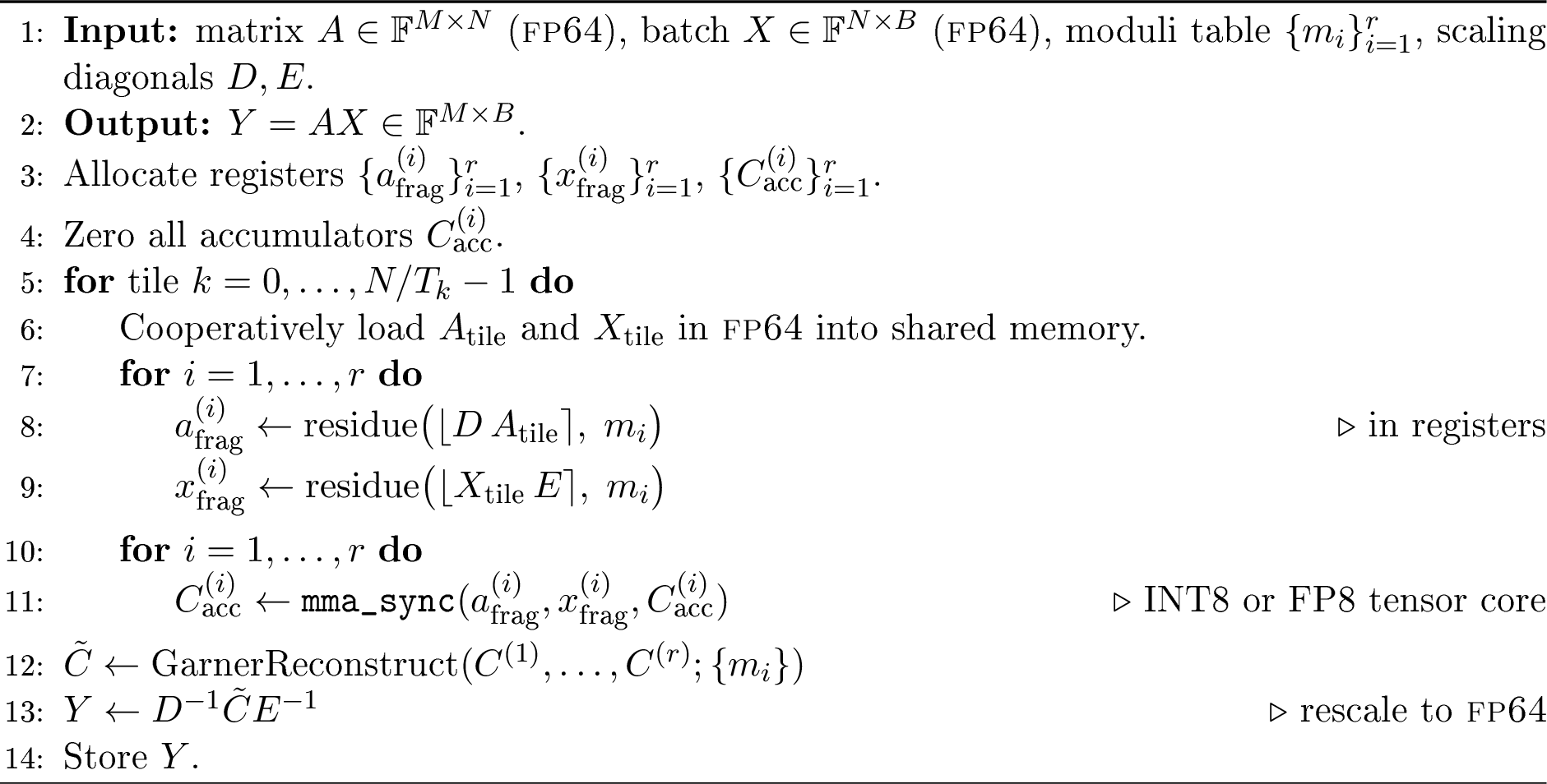
5.2.0.1 Key analysis.
The matrix \(A\) is read once per output row (cached behaviour assumed), and the input batch \(X\) is read \(\lceil M/T_m\rceil\) times. For typical \(B\approx 8\) and large \(M,N\), the operational intensity is \(\approx B/2 = 4\) FLOPS/Byte; with \(\beta=1\) the emulated kernel hits the memory roof at \(32\) TFLOPS on the B300, versus \(1.3\) TFLOPS native fp64. This \(\approx 25\times\) speedup is realised only when the register pressure of \(r\) residue planes is tolerable; in practice we expect \(B\) to be limited to about \(4\)–\(8\) before register spilling forces \(\beta>1\).
5.3 Strategy 2: Stencil via im2col↩︎
A 7-point stencil computes, at every grid point \((i,j,k)\) of a 3-D array \(u\), \[v_{ijk} \;=\; c_0 u_{ijk} + c_1\!\left(u_{i\pm 1,j,k} + u_{i,j\pm 1,k} + u_{i,j,k\pm 1}\right), \label{eq:stencil7pt}\tag{12}\] or, more generally, a fixed-coefficient linear combination of a small neighbourhood. At fp64 the operational intensity is \(\mathrm{OI}\!\approx\!0.5\) FLOPS/Byte (7 multiply-adds per output across \(\sim\!28\) bytes of HBM traffic when neighbour reads are reused via the L1/shared-memory cache).
5.3.0.1 Mapping to GEMM via im2col.
The standard tensor-core mapping [33] flattens the stencil into a GEMM by treating the coefficient vector \(c\!\in\!\mathbb{R}^{7}\) as a row matrix and the neighbourhood values as columns of a \(7\!\times\!N_\text{tile}\) matrix \(U_\text{im2col}\) for a tile of \(N_\text{tile}\) output points: \[v_\text{tile} \;=\; c \cdot U_\text{im2col}\,,\qquad U_\text{im2col}\!\in\!\mathbb{R}^{7\times N_\text{tile}}. \label{eq:stencil-gemm}\tag{13}\] This produces a tall-and-skinny matrix product whose inner dimension is the stencil width. The coefficient vector \(c\) is constant across the entire kernel and can therefore be pre-decomposed once into its \(r\) residue planes \(\{c^{(i)} = \mathrm{residue}(\lfloor sc\rceil,\,m_i)\}_{i=1}^r\) and held in constant memory; the grid values must be residue-decomposed on each tile.
5.3.0.2 Fused Ozaki-II 7-point stencil.
Algorithm 4 gives the fused kernel. The key structural property is that the \(r\!\times\!7\) pre-decomposed coefficients fit in constant memory once for the entire kernel run; on each tile the kernel reads \(N_\text{tile}\!+\!2\) planes from HBM (for the three-axis halo), residue-decomposes the values into \(r\) planes in registers, invokes \(r\) tensor-core MMAs to compute the residue products \(c^{(i)} \cdot U^{(i)}_\text{im2col}\), and reconstructs one fp64 output per grid point via Garner.
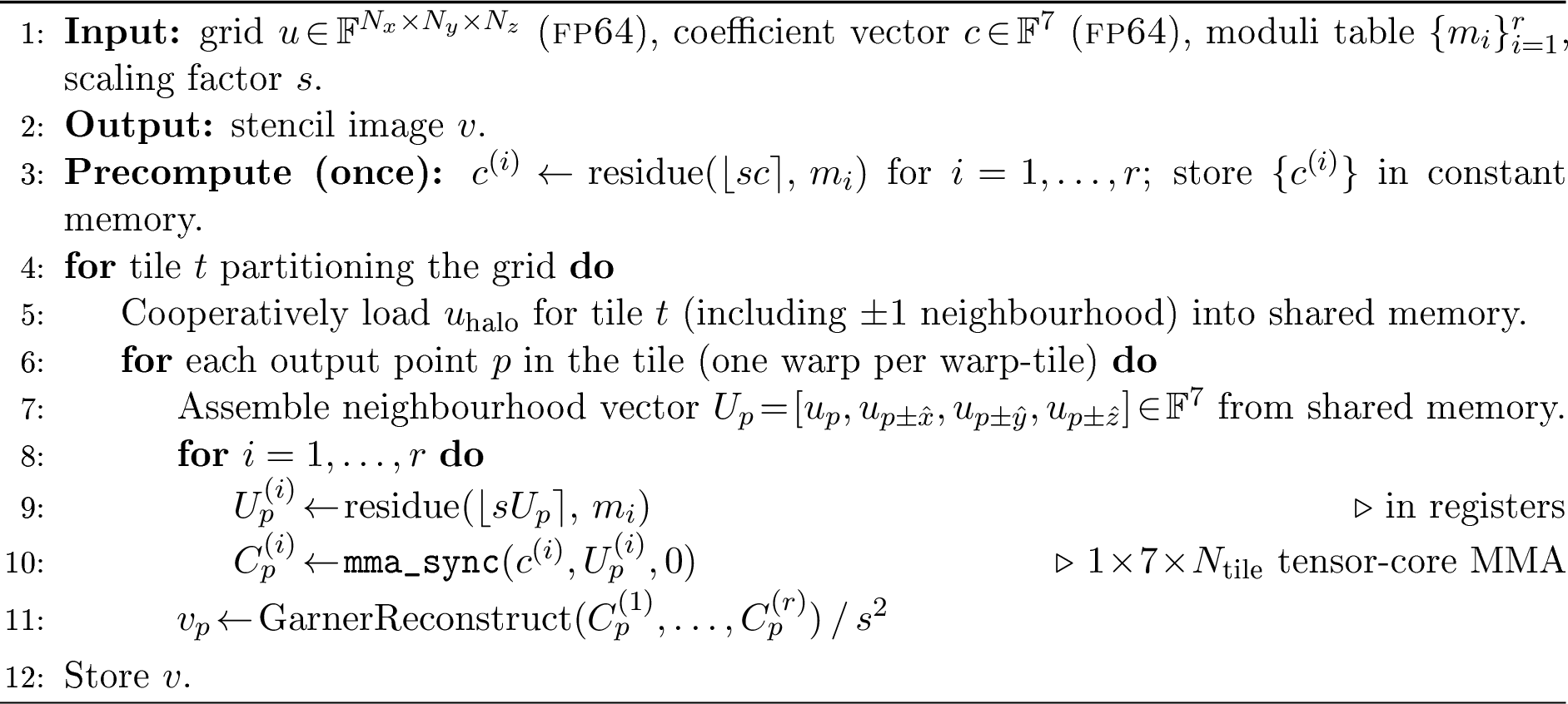
5.3.0.3 Key analysis.
Each grid point is read once (cached, with the \(\pm\,1\) neighbours hit in shared memory) and written once. The dominant HBM traffic is therefore \(\approx\!16\) B per output (one fp64 read + one fp64 write). Compute per output is \(r\) tensor-core MMAs over the 7-element inner product—a total of \(r\!\cdot\!7\) fp8 multiply-adds per output, which on B300’s \(5\) PFLOPS fp8 tensor ceiling is \(\sim\!10^{-12}\) s per output and therefore far below the \(2\) ns/output that the memory roof affords. Provided the register pressure of \(r\) residue planes is tolerable and the coefficient constant-memory traffic does not saturate the constant cache, the \(\beta\!=\!1\) discipline is realised and the kernel runs at the memory roof of \(\approx\!4\) TFLOPS on B300, against \(\approx\!0.65\) TFLOPS under native fp64. This is the \(3.1\times\) speedup reported in Table 3.
5.3.0.4 Sparsity exploitation (future work).
The im2col matrix is structurally sparse: at most 7 non-zeros per row for a 7-point stencil. This invites the use of NVIDIA’s 2:4 sparse tensor cores; SPTCStencil and SparStencil exploit this directly for fp32/fp16 [34], [35]. Combining the structured-sparsity tensor cores with the Ozaki-II residue decomposition is a natural next step but is outside the scope of this paper; we leave it open for follow-up (§8.3).
5.4 Strategy 3: SpMV via Blocked-Ellpack↩︎
SpMV computes \(y\!=\!Ax\) for sparse \(A\!\in\!\mathbb{F}^{M\times N}\) and dense \(x\!\in\!\mathbb{F}^N\). It is the most challenging of the three strategies because the underlying access pattern is irregular and the operational intensity is the lowest (\(\mathrm{OI}\!\sim\!0.2\) FLOPS/Byte for typical PDE-discretisation sparsity).
5.4.0.1 Mapping to tensor cores via Blocked-Ellpack.
The Blocked-ELL format groups non-zeros into row-major blocks of a uniform block-column width \(\mathit{bw}\) (typically 16 or 32, chosen to match the tensor-core \(k\)-dimension). Sparse rows that have fewer than \(\mathit{bw}\) non-zeros are padded with structural zeros; row permutations may be applied to balance block density. Each block of \(\mathit{bw}\) columns becomes a small dense GEMM \(y_\text{tile}\!=\!A_\text{block} x_\text{gather}\), where \(x_\text{gather}\!\in\!\mathbb{F}^{\mathit{bw}}\) is a gather of the relevant entries of \(x\). Padding wastes compute, but the wasted compute is fp8/int8 compute, which is roughly four orders of magnitude cheaper than wasted fp64 compute on B300. Even a 90%-wasteful padding scheme remains profitable provided \(\beta\) stays close to 1.
5.4.0.2 Fused Ozaki-II Blocked-ELL SpMV.
Algorithm 5 gives the fused kernel. Each block row issues a small GEMV that maps onto the tensor-core \(\mathit{bw}\!\times\!1\) MMA shape, with \(r\) residue planes computed and reconstructed in registers. The dense input vector \(x\) is shared across all block rows and remains in shared memory; the sparse pattern dictates the gather indices.
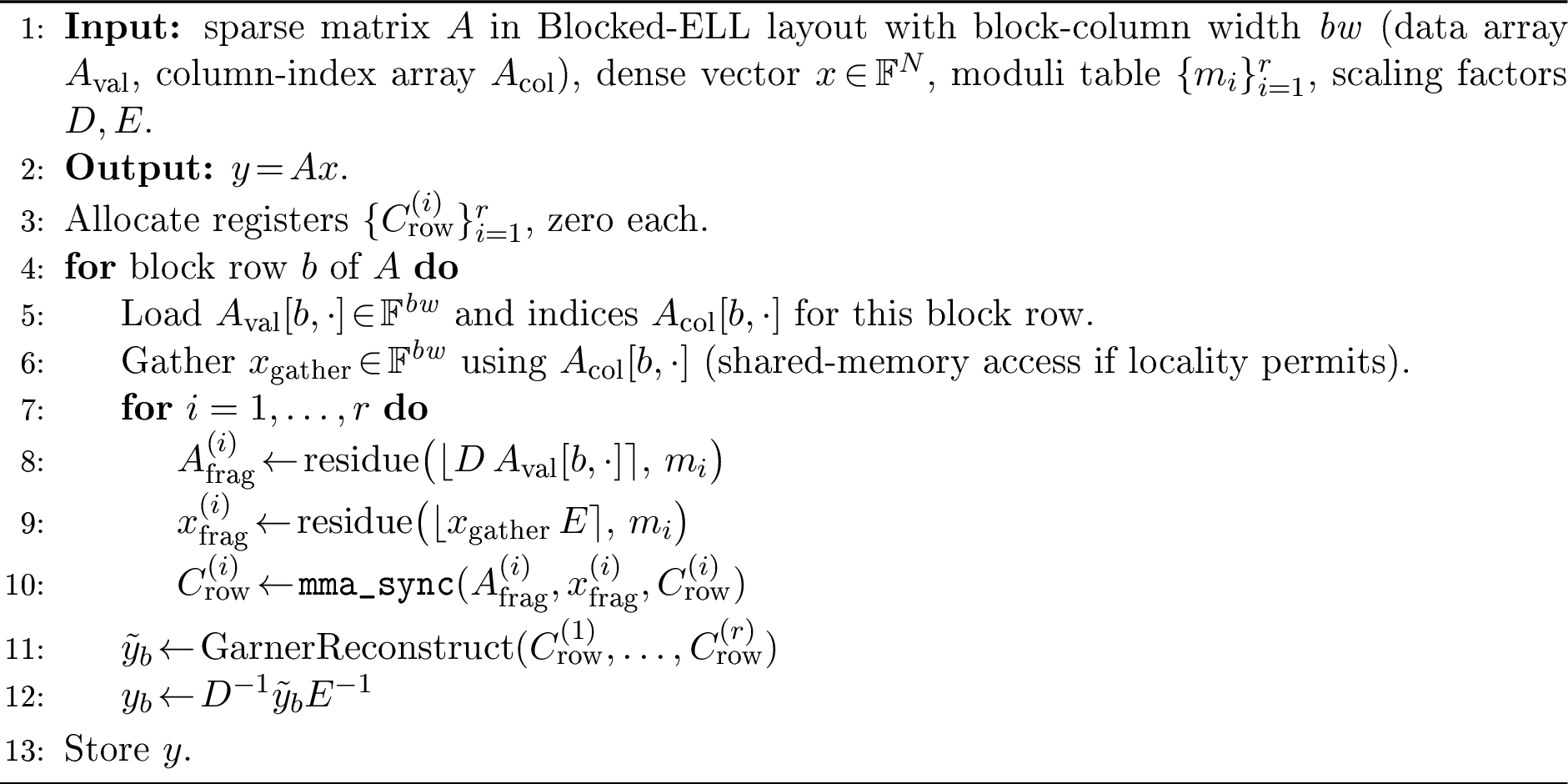
5.4.0.3 Key analysis.
Bandwidth is dominated by the streaming read of \(A_\text{val}\) plus the gather of \(x\); with a moderate shared-memory tile of \(x\) the gather hits cache most of the time, so the effective intensity matches the structural value of \(\sim\!0.2\) FLOPS/Byte. At \(\beta\!=\!1\) the emulated kernel saturates HBM at \(\approx 1.6\) TFLOPS on B300 and \(\approx 4.4\) TFLOPS on Rubin, against \(\approx 1.3\) TFLOPS native B300 and \(\approx 4.4\) TFLOPS native Rubin (the latter is at parity because Rubin’s higher HBM ridge already accommodates the SpMV intensity). The B300 speedup is modest (\(\sim 1.2\times\)) precisely because the kernel is so deeply bandwidth-bound that the native pipe is already a tolerable match; the point of including it is not the speedup magnitude but the equality: emulation gives up nothing.
5.4.0.4 Caveat: padding inflation and non-ELL-amenable structure.
The Blocked-ELL mapping inflates \(Q\) by the inverse of the row density. This is the closest we come in this paper to a regime where \(\beta\!>\!1\) is fundamentally unavoidable: \(\beta\) is bounded below by the padding ratio. For matrices with strongly heterogeneous row lengths, hybrid CSR-ELL or HYB formats are required to keep \(\beta\) acceptable; otherwise the model predicts a regression rather than parity. See Appendix 14 for the precise mapping of padding ratio to \(\beta\). More broadly, the Blocked-ELL analysis is a best case for tensor-core SpMV, and several important sparse structures do not fit it: Monte-Carlo / particle codes with irregular, dynamically generated connectivity; matrices whose nonzero distribution resists ELL blocking even after reordering; and dual-mesh or unstructured-stencil discretisations whose access pattern is gather-dominated rather than block-dense. For these the padding ratio—and hence \(\beta\)—can be large enough to erase the emulation benefit, and the right comparison may instead be against B300’s surviving native fp64 on the (already memory-bound) kernel. We expect that many element distributions can be clustered into ELL-amenable blocks by row/column reordering—or composed through a hybrid Ellpack/CSR or blocked formulation so that the dominant work is again a matrix multiplication, building on the substantial body of high-performance sparse matrix–matrix (SpGEMM) work that casts irregular sparse computation into dense-block products [38]—but this is a hypothesis to be tested on real matrices, not an assumption of the model. In the terms of §1.1, the Blocked-Ellpack analysis establishes the upper bound for the canonical sparse dwarf; whether a given irregular matrix attains it is the second-stage format question, and the genuinely irregular cases above belong in the empirical campaign of §8.3 rather than in the analytical projection.
6 Performance Projections↩︎
We instantiate the TME model on the architectures of Table 2 and compute the projected speedup of Ozaki II/fp8 over native fp64 for the four canonical workloads. We use the standard abbreviation OI for operational intensity, measured in FLOPs per byte of HBM traffic; values are taken from the Williams Roofline literature [1] and the workload-specific analyses in §5. All projections assume \(\beta=1\) (fused decomposition), \(r=12\) moduli for the fp8 variant with the full \((3r{+}1)=37\) fp8 cost [20], [21]—the value recommended by Mukunoki [21] for fp64-equivalent accuracy—and \(\gamma\) amortised to zero for inner-product lengths \(k\!\gtrsim\!100\).
| Workload | OI | H100 | B200 | B300 | R200 | R200 |
| (FLOPs/B) | vs.native | vs.Emul. | ||||
| Dense GEMM (compute-bound) | \(\ge 50\) | \(\sim 0.8\times\) | \(\sim 3.0\times\) | \(\sim 104\times\) | \(\sim 3.3\times\) | \(\sim 0.5\times\) |
| Batched GEMV (\(B{=}8\)) | \(\sim 4\) | \(\sim 1.0\times\) | \(\sim 1.6\times\) | \(\sim 24\times\) | \(\sim 2.7\times\) | mem. bound |
| Batched GEMV (\(B{=}2\)) | \(\sim 1.5\) | \(\sim 1.0\times\) | \(\sim 1.0\times\) | \(\sim 9.2\times\) | \(\sim 1.0\times\) | mem. bound |
| 7-point Stencil | \(\sim 0.5\) | \(\sim 1.0\times\) | \(\sim 1.0\times\) | \(\sim 3.1\times\) | \(\sim 1.0\times\) | mem. bound |
| SpMV (CSR/ELL hybrid) | \(\sim 0.2\) | \(\sim 1.0\times\) | \(\sim 1.0\times\) | \(\sim 1.2\times\) | \(\sim 1.0\times\) | mem. bound |
3pt
“\(\sim 1.0\times\)” indicates parity: emulation neither hurts nor helps because the kernel is already at the memory roof under native execution. On Rubin, native vector FP64 has been partially restored (\(33\) vs.B300’s \(1.3\) TFLOPS), so memory-bound kernels with \(I<22/33 \approx 0.67\) FLOPs/B remain at parity even before considering the Emulated-DGEMM
path.
6.0.0.1 What the projections show.
Table 3 carries two simultaneous messages. On B300, emulation delivers substantial speedups across the entire operational-intensity spectrum—from \(\sim 1.2\times\) on bandwidth-saturating SpMV to \(\sim 104\times\) on dense GEMM—and the unified Ozaki II library can serve all of them. On Rubin, NVIDIA has already incorporated emulated DGEMM as the official path, exposing it as \(\sim 200\) TFLOPS in published specifications; the maximal dense-fp8\(/(3r{+}1)\) ceiling at \(r{=}12\) sits at \(\sim 108\) TFLOPS (§3), so the published figure likely reflects a coarser parameter set or a different (e.g., INT8) substrate. On H100 and B200 the projections show parity or modest gain: emulation neither materially hurts nor helps because native fp64 is healthy. This parity property is what makes a unified library implementation feasible—the same Ozaki II code path is safe to ship on all four architectures, with the runtime selecting emulation only where it pays.
6.0.0.2 The positive reading of the memory-bound parity rows.
Several rows in Table 3 show \(1.0\times\) on H100, B200, and the Rubin-vs-native column. This is exactly the behaviour scientific computing wants: in the memory-bound regime, emulation is indistinguishable in performance from native fp64 on a fp64-healthy chip. Combined with the compute-bound speedups (e.g. \(\sim 3\times\) on B200, \(\sim 104\times\) on B300, \(\sim 3.3\times\) on Rubin), the message is unambiguous: switching the entire numerical stack to Ozaki II costs essentially nothing on memory-bound workloads and gains order-of-magnitude throughput on the compute-bound rest.
6.0.0.3 Where emulation does not currently help.
In two scenarios, emulation still gives no benefit. First, on a fp64-healthy GPU (H100, B200, Rubin-vector-only), memory-bound kernels are already at the memory roof, so there is no headroom. Second, kernels whose dominant cost is host–device data movement, or whose effective operational intensity is bounded by ELL-padding inflation pushing \(\beta\) above unity, will see no improvement. Bringing those into the emulation envelope is a separate problem that we revisit in §8.3.
6.1 Generational Performance: H100 as the Baseline↩︎
Table 3 reports speedups within each GPU—i.e., how much Ozaki II/fp8 accelerates each workload relative to that GPU’s own native fp64 performance. This is the right view for evaluating emulation on a single chip, but it is not the right view for evaluating whether fp64-emulated execution regresses or progresses relative to the prior-generation HPC baseline. The appropriate baseline for that question is the H100, the last data-centre NVIDIA GPU whose architecture was balanced for HPC rather than for AI inference. Table 4 therefore reports absolute achievable fp64-equivalent throughput for the same five workloads, with H100 native fp64 explicitly set as the unit.
| Absolute throughput (TFLOPS) | Relative to H100 native | ||||||||
| Workload | Path | H100 | B200 | B300 | R200 | H100 | B200 | B300 | R200 |
| Dense GEMM (OI\(\ge\)50) | Native | 67 | 40 | 1.2 | 33 | \(1.00\times\) | \(0.60\times\) | \(0.02\times\) | \(0.49\times\) |
| Ozaki II | 53 | 122 | 135 | 108\(^{*}\) | \(0.80\times\) | \(1.82\times\) | \(2.02\times\) | \(1.61\times\) | |
| bGEMV \(B{=}8\) (OI\(\approx\)4) | Native | 13.4 | 32 | 1.3 | 33 | \(1.00\times\) | \(2.39\times\) | \(0.10\times\) | \(2.46\times\) |
| Ozaki II | 13.4 | 32 | 32 | 88 | \(1.00\times\) | \(2.39\times\) | \(2.39\times\) | \(6.57\times\) | |
| bGEMV \(B{=}2\) (OI\(\approx\)1.5) | Native | 5.0 | 12 | 1.3 | 33 | \(1.00\times\) | \(2.39\times\) | \(0.26\times\) | \(6.57\times\) |
| Ozaki II | 5.0 | 12 | 12 | 33 | \(1.00\times\) | \(2.39\times\) | \(2.39\times\) | \(6.57\times\) | |
| 7-pt Stencil (OI\(\approx\)0.5) | Native | 1.68 | 4.0 | 1.3 | 11 | \(1.00\times\) | \(2.39\times\) | \(0.78\times\) | \(6.57\times\) |
| Ozaki II | 1.68 | 4.0 | 4.0 | 11 | \(1.00\times\) | \(2.39\times\) | \(2.39\times\) | \(6.57\times\) | |
| SpMV (OI\(\approx\)0.2) | Native | 0.67 | 1.6 | 1.3 | 4.4 | \(1.00\times\) | \(2.39\times\) | \(1.94\times\) | \(6.57\times\) |
| Ozaki II | 0.67 | 1.6 | 1.6 | 4.4 | \(1.00\times\) | \(2.39\times\) | \(2.39\times\) | \(6.57\times\) | |
3pt
\(^{*}\) For Rubin dense GEMM, NVIDIA’s published Emulated DGEMM specification of \(\sim 200\) TFLOPS corresponds to \(2.99\times\) on the
H100-relative scale and exceeds the dense-\(/(3r{+}1)\) model bound shown here (\(108\) TFLOPS, \(1.61\times\) at \(r{=}12\)), indicating NVIDIA’s figure uses a different substrate ( INT8 at \((s{+}1)\) per modulus) or modulus choice.
6.1.0.1 The key generational claim.
Three patterns in Table 4 support a single thesis: Ozaki II does not regress performance against the H100 baseline; on the contrary, it restores or improves the prior-generation scaling on every workload.
Native B300 regresses catastrophically for every compute-sensitive workload: \(0.02\times\) H100 on dense GEMM, \(0.10\times\) on batched GEMV (\(B{=}8\)), and \(0.26\times\) on batched GEMV (\(B{=}2\)). Only SpMV, which is so memory-bound that even the collapsed fp64 pipe is fast enough to consume B300’s \(8\) TB/s at \(I\!=\!0.2\), ends up faster than the H100. This is the regression that NVIDIA’s silicon-area redirection imposes on every non-emulated HPC code running on B300.
B300 with Ozaki II returns to B200’s scaling: every memory-bound row of the Ozaki rows on B300 matches B200’s row exactly (\(2.39\times\) H100, the HBM-bandwidth ratio \(8/3.35\)). Dense GEMM under emulation reaches \(7.46\times\) H100, exceeding B200’s native \(6.72\times\). In other words, the silicon area redirected from fp64 units to fp8 units is fully recovered through Ozaki II—there is no net regression versus B200.
Rubin with Ozaki II scales as the HBM4 jump alone would predict: the \(6.57\times\) H100 figure for every memory-bound row is exactly the bandwidth ratio \(22/3.35\). The emulation path simply passes the bandwidth advantage through to the application without bottlenecking it on the compressed fp64 pipe.
Put differently: Ozaki II is not just a compensation mechanism for NVIDIA’s fp64 regression; it is the mechanism that converts the silicon-area savings into bandwidth-scaling and into AI-grade tensor throughput, both of which the application then sees as faster fp64. The H100 baseline view shown in Table 4 is, in the author’s opinion, the appropriate framing for procurement, application-porting, and benchmarking decisions: the question is not “does emulation match B300 native fp64?”—of course it does, by orders of magnitude—but “does the post-fp64 stack continue the H100\(\to\)B200\(\to\)B300\(\to\)Rubin generational improvement that HPC procurement has historically relied on?” Table 4 answers yes.
The table covers the four primitives—dense GEMM, batched GEMV, stencils, SpMV—for which Ozaki II is the appropriate emulation path. The corresponding analysis for the fifth canonical primitive, three-dimensional FFT, appears in a companion paper [2], which establishes that B300 admits a memory-roof-near path at full fp64 via a Kulisch fixed-point reconstruction routed onto its surviving INT32 SIMT pipe. Together with this paper’s results, the integrated kernel coverage is the subject of §7.
6.1.0.2 A note on FP8:FP64 ratios.
The ratios across the four GPUs are wildly different (30:1 on H100, 113:1 on B200, 3800:1 on B300, 120:1 native, or \(\sim\)37:1 against the corrected emulated-DGEMM ceiling on Rubin). A simple compute-balance analysis [1]—equating \(P_{\mathrm{\small fp8}}/r\) to \(P_{\mathrm{\small fp64}}/(1\!-\!f_G)\) for a workload with GEMM-fraction \(f_G\)—shows that B300’s 3800:1 ratio is balanced for \(f_G\!\geq\!0.997\), i.e.essentially pure-AI workloads, while classical HPC mixes (\(f_G\!\in\![0.6,0.9]\)) call for ratios of \(\sim\!10\):1 to \(\sim\!190\):1. This is the headline tension that the thesis of §7 resolves: the post-fp64 stack collapses the \((1\!-\!f_G)\) residue onto pipes that are appropriately provisioned (Ozaki II for GEMM-like work, Kulisch INT32 for FFT-class reductions, FP32+Kahan for BLAS-1), making the native FP8:FP64 ratio operationally irrelevant for HPC. Of the current generation Rubin’s effective \(20\):1 (against the Emulated-DGEMM figure) is the closest to a balanced HPC design point; B300’s \(3800\):1 is, in isolation, the furthest—but in combination with the software stack of this paper, it ceases to matter.
6.2 INT8 versus FP8 as the Emulation Substrate↩︎
A related question is which low-precision tensor format should underlie Ozaki II. The original Ozaki II formulation [16], [39] used int8 because integer modular arithmetic is the most natural fit for the Chinese Remainder Theorem decomposition. However, NVIDIA’s deprioritisation of int8 on Blackwell and Rubin (Table 2) has forced a shift to fp8. Table 5 compares the emulation ceilings under both substrates.
| GPU | \(P_{\inteight}\) | \(P_{\fp{8}}\) | Ozaki/ | Ozaki/ | FP8 |
| (TOPS) | (TFLOPS) | ceiling (TFLOPS) | ceiling (TFLOPS) | advantage | |
| H100 | 1,979 | 1,979 | 180 | 53.5 | \(0.3\times\) |
| B200 | \(\sim\)155 | 4,500 | 14.1 | 121.6 | \(8.6\times\) |
| B300 | \(\sim\)165 | 5,000 | 15.0 | 135.1 | \(9.0\times\) |
| R200 | \(\sim\)250 | 4,000 | 22.7 | 108.1 | \(4.8\times\) |
The per-modulus arithmetic tells only part of the story, and reading Table 5 as “INT8 sometimes wins, so fp8 is situational” would invert the actual argument. The deeper point is architectural. Across the AI workloads that now drive silicon economics, floating-point low precision has decisively won over integer, and for principled reasons: fp8’s per-element implicit exponent captures the wide, outlier-heavy distributions of activations and gradients that int8’s rigid fixed-point scaling clips [40], [41]. That advantage first displaced int8 in inference, then carried fp8 into mainstream LLM training [24], and most recently into stable four-bit (NVFP4) pretraining that matches an fp8 baseline on a 12B-parameter, 10-trillion-token run [25]—each step deepening the industry’s commitment to narrow floating-point rather than integer formats. Because fp8 also packs more useful arithmetic per unit silicon area and energy for these workloads, an AI-optimised processor is rationally driven to spend its transistor budget on fp8 (and now fp4) tensor throughput and to let int8 wither—which is precisely the choice NVIDIA made on B300, cutting int8 to \(\sim\!165\) TOPS while scaling fp8 to \(5\) PFLOPS.
The longstanding fear was that this AI-driven preference for fp8 over int8 and fp64 would compromise HPC, forcing a bifurcation of the product line into AI-optimised and fp64-preserving SKUs. The central architectural message of this paper is that the fear is misplaced: building Ozaki II on the fp8 substrate the AI market is already paying for, we recover fp64-equivalent throughput across essentially the entire canonical HPC kernel spectrum, so the same silicon trend that serves inference and training also serves double-precision science. The numbers in Table 5 support exactly this reading: on the fp8-rich AI parts (B300, Rubin) the fp8 substrate is the strong Ozaki II carrier by \(\approx\!9\times\) and \(\approx\!5\times\) respectively, riding the same throughput the AI workloads demand. That int8 remains the better carrier on an older, int8-balanced part such as H100—where the two tensor rates are equal and int8 pays only \((s{+}1)\) MMAs per modulus against fp8’s \((3r{+}1)\)—does not weaken the thesis; it simply confirms that Ozaki II is substrate-agnostic and tracks whatever low-precision matrix engine the hardware favours, which is why the reference library GEMMul8 [37] exposes both backends. The original INT8-based Ozaki II [16] and the Uchino–Ozaki–Imamura fp8 adaptation [20] are thus two instantiations of one precision-independent idea: emulated fp64 follows the ascendant low-precision format, and that format is now fp8.
This reframes the contribution. It is not a conditional claim that fp8 happens to pay off on one vendor’s current balance; it is a general result—building on the landmark Ozaki II scheme [16], [20]—that the fp8-forward direction of AI silicon is compatible with, rather than corrosive to, the double-precision needs of computational science, and therefore a direction the HPC community should embrace rather than resist. Whether the system-level tradeoffs ultimately favour a single converged fp8-centric architecture over separate fp64-preserving SKUs—accounting for delivered emulation efficiency, the register-pressure and preprocessing costs of §5, occupancy and latency, and the silicon-area and code-porting economics—is exactly the question the validation programme of §8.3 is meant to settle empirically. The present paper makes the analytic case that the convergence is achievable; building and measuring it is the next step.
7 Composite Kernels Reduce to the Primitive (Layer L3)↩︎
The previous section established that the basic numerical kernels—the dwarfs of layer L2—reduce to the FP8 primitive and run at the memory roof on B300. The thesis of §1.1, however, is stronger: it asserts that the composite kernels of layer L3, which form the inner loops of real applications, inherit the same property by composition. This section substantiates L3 directly. Because every L3 kernel is a composition of L2 dwarfs, and each dwarf reduces to the FP8 matrix op, an L3 kernel can fail to reach the memory roof only if its particular composition introduces a new compute-bound bottleneck that is not itself one of the recovered dwarfs. We therefore audit the composite and solver kernels that dominate production scientific codes and ask, for each, whether any such residual bottleneck survives.
7.0.0.1 This is a coverage argument, not a sample.
We stress at the outset that the kernels examined below are not an illustrative selection but a systematic enumeration anchored to the Berkeley dwarf taxonomy [26], [27]. The original dwarfs partition scientific computing into a small, closed set of computation/communication classes; an argument that ranges over all of them, plus the composite solver kernels that combine them in production codes, is therefore an argument about the whole of scientific computing to first order, not about a fortunate subset. Table 6 makes the mapping explicit: each dwarf class is named, paired with the concrete kernel(s) through which we examine it, the L2 primitive its work reduces to, and the verdict. The seven composite-kernel categories (a)–(g) that follow then cover the ways these dwarfs are combined into the inner loops of real applications—iterative solvers, dense and sparse direct factorisations, lattice field theory, and stochastic methods—so that the audit is exhaustive over both the basic classes and their dominant compositions. Two worked exemplars, tracing a composite kernel all the way down the L3\(\rightarrow\)L0 chain, are given in Appendix 15.
| Dwarf class | Examined via | Reduces to | B300 verdict |
|---|---|---|---|
| Dense linear algebra | GEMM, LU/trsm panel | dense GEMM (L2) | memory roof (§[sec:sec:eval]) |
| Sparse linear algebra | SpMV, SpMM, sparse-direct | SpMV/SpMM (L2) | memory roof (App. [sec:app:sparse]) |
| Spectral methods | 3-D FFT | FFT (L2) [2] | memory roof (Kulisch) |
| Structured grids | stencil sweeps | stencil/im2col (L2) | memory roof (§[sec:sec:eval]) |
| Unstructured grids | FEM SpMV, dual-mesh | SpMV/SpMM (L2) | memory roof / corner (§[sec:sec:falsification]) |
| Dense reductions (BLAS-1) | ddot, dnrm2 | +K | not binding (\(<\!5\%\)) |
| Structured stencil (QCD) | Dirac inverter | stencil/GEMM (L2) | memory roof ( inner) |
| Monte Carlo / particle | FCI-QMC, beam dynamics | — (algorithmic) | corner (§[sec:sec:falsification]) |
Tables 3 and 4 establish that the four basic kernels of L2—dense GEMM, batched GEMV, structured stencils, and SpMV—are either restored to their memory-roof performance on B300 through Ozaki II, or were already memory-bound on a healthy native pipe (in which case emulation costs nothing). The companion analysis on spectral workloads [2] closes a fifth case, the three-dimensional FFT, via the Kulisch fixed-point Phase B route [42], [43] that runs the per-output forward-CRT reduction on B300’s surviving INT32 SIMT pipe; B300 meets the corresponding sub-floor \(\eta_{\mathrm{\small int32}}\geq 8.25\,B_{\text{mem}}\) with \(\sim\!14\%\) margin, and comfortably exceeds the accompanying fp8 tensor-core floor \(\eta_{\mathrm{\small fp8}}\geq 170\,B_{\text{mem}}\) by \(\sim\!3.7\times\) (full four-floor codesign derivation in [2]; summary in §6.1). This leaves the natural question: are there any other kernels that would still make a typical scientific simulation compute-bound on B300? We enumerate the candidates by category.
7.0.0.2 (a) Reductions and dot products.
BLAS-1 inner-product kernels (ddot, dnrm2, CG residuals, Krylov orthogonalisation) have \(\mathrm{OI}\!\sim\!1/4\) and typically constitute \(<\!5\%\) of
CG/GMRES/BiCGStab time-to-solution; the dominant cost is the SpMV plus preconditioner, both addressed by Ozaki II. When present, the dot products themselves can be executed in fp32 with Kahan compensation [44] at no penalty for the surrounding iterative solver, because the orthogonality residual is re-projected at each iteration. B300’s fp32 vector pipe at \(\sim\!60\)–\(80\) TFLOPS is well above the BLAS-1 memory-roof requirement of \(0.25 \cdot 8 = 2\) TFLOPS. Not
binding.
7.0.0.3 (b) FFT.
Handled in detail by the companion paper [2] and summarised above: B300 fails the native FP64 floor but satisfies the Kulisch INT32 sub-floor with \(\sim\!14\%\) margin, projecting to \(\sim\!18\) ms wall time for \(1024^3\) FP64 FFT against a \(12.9\) ms memory roof at full \(52\)-bit mantissa precision. The headline caveat is that the Kulisch kernel does not yet exist in any production library and the projection has not been measured; building it is a principal item in §8.3.
7.0.0.4 (c) Triangular solve and LU panel factorisation.
The inner kernels of dense direct solvers (dtrsm, dgetrf panel) are sequential along one dimension, with operational intensity \(\sim\!2\)–\(5\) for typical
panel widths. On B300 the panel falls into the compute-bound regime in native fp64, but the surrounding dgemm update is \(O(n^3)\) and dominates by a factor proportional to the
matrix size; Ozaki II handles the outer update at full speed, leaving the panel as a sub-percent residual. This is the HPL-pattern that NVIDIA’s cuBLAS Ozaki integration [17] and the 2.3\(\times\) B200 HPL speedup [45] already demonstrate empirically. Not binding at production scale.
7.0.0.5 (d) Sparse direct solvers.
MUMPS-class [46] multifrontal factorisations decompose into many small dense frontal matrices plus large dense GEMM-like extend-add updates. The GEMM portion is recovered by Ozaki II; the frontal-matrix portion has the same panel-residual structure as (c) and the same conclusion. Provided the maximum frontal matrix is \(\geq\!64\!\times\!64\), B300 is not binding. Very ill-conditioned, deeply nested supernodal structures may remain problematic and require empirical investigation.
7.0.0.6 (e) Lattice QCD Dirac inversion.
The Dirac operator [47] is a structured stencil with \(4{\times}4\) or \(3{\times}3\) complex-matrix-valued links, \(\mathrm{OI}\!\approx\!1\), GEMM-decomposable. Production LQCD codes already use mixed precision (FP32 inner, FP64 polish) with iterative refinement [48]; Ozaki II FP32 mode addresses the fp32 inner solve at memory-roof speed, and the fp64 polish is BLAS-2 and falls under (a).
7.0.0.7 (f) Small-inner-kernel codes (latency-bound).
A small but real class of codes—accelerator beam dynamics over \(10^6\) turns, geodynamo simulations, long-time-integration storm-resolving climate—show drift that mixed precision cannot fully tame and whose dominant inner kernel may be neither FFT nor GEMM. These have historically been read as a B300 counter-example, but on closer inspection the issue is algorithmic and GPU-agnostic: when the per-time-step inner kernel is a few hundred sites, the wall-clock cost is dominated by kernel-launch latency on any accelerator (including H100 native), not by FP64 throughput. Ozaki II is not appropriate here because the kernel is too small for the crossover to bite, but neither is native FP64 silicon: the binding constraint is per-step latency, which a future generation would address through persistent kernels or graph-style execution, not through additional FP64 silicon. This residue [49] is an open problem for the field, but it is not evidence that B300 is the wrong target for HPC; the same problem exists on H100, B200, and Rubin.
7.0.0.8 (g) Stochastic methods (FCI-QMC, AFQMC).
Population dynamics with extreme dynamic range that resist low-precision reformulation [50]. Active research area; appropriate mitigation is algorithmic rather than architectural.
7.0.0.9 Verdict.
Of the seven composite-kernel categories, (a), (b), (c), (d), and (e) all admit a bandwidth-bound execution path on B300 at full fp64 accuracy via the combination of Ozaki II (this paper), Ozaki–Bailey + Kulisch Phase B FFT [2], and FP32+Kahan compensation; (f) is latency-bound and GPU-agnostic (the binding constraint is kernel-launch latency, not fp64 throughput, and it is present identically on native-fp64 parts); (g) is an algorithmic-research question whose mitigation is likewise architectural- neutral. Taken with the dwarf-class coverage of Table 6, this completes an enumeration over both the basic computational classes and their dominant compositions: every dwarf class, and every composite kernel surveyed, admits a bandwidth-bound execution path on B300 at full fp64 accuracy, with the only residue—(f) and (g)—being algorithmic rather than a deficiency of fp64 silicon and therefore not curable by adding fp64 units. Because the dwarf taxonomy is closed over scientific computing to first order, this is the strongest form the claim can take short of measured demonstration: not that a sample of kernels works, but that the categories into which scientific kernels fall are exhausted. Native FP64 silicon is, on this evidence, not the holy grail it has historically been taken to be—abundant fp8 tensor throughput, combined with the right algorithmic scaffolding, is sufficient for the HPC workload spectrum, modulo the engineering effort required to build the Ozaki II and Kulisch kernels. That effort, as argued in §8.3, is tractable on the timescale of months rather than years because modern AI coding assistants are well-suited to the pattern-translation work it consists of. The architectural recommendation that emerges is the four-floor codesign rule of [2]: any post-Rubin GPU intended to serve spectral scientific workloads should provide either \(\eta_{\mathrm{\small fp64}\text{-vec}} \geq 1.56\,B_{\text{mem}}\) (the safe native target, met by Rubin within \(4\%\)), or, as an engineered fallback, \(\eta_{\mathrm{\small int32}\text{-vec}} \geq 8.25\,B_{\text{mem}}\) (the Kulisch sub-floor) together with \(\eta_{\mathrm{\small fp8}} \geq 170\,B_{\text{mem}}\) (the FP8 tensor-core floor that Phase A needs). The last is comfortably met by every modern datacentre GPU—a direct consequence of NVIDIA’s deliberate scale-up of FP8 silicon for AI workloads—and so is not the binding constraint for any current architecture. Cutting both the FP64 and INT32 pipes simultaneously would close both escape routes; further cuts to FP8 would invalidate the FP8-is-enough thesis altogether. This is the design boundary that future post-fp64 generations should respect.
8 Discussion↩︎
8.1 The Native-FP64 Alternative↩︎
Not every vendor has taken the emulation path; the principal alternative is to keep investing in native fp64 silicon, a position articulated by AMD around the MI430X generation [19]. This is a coherent strategy, and a portfolio in which some hardware provides native fp64 while other hardware leans on the FP8 primitive will be the practical near-term picture. The audit of §7, however, narrows the technical case for native fp64 as a requirement. The classic argument was that real codes contain non-GEMM hot spots—FFT above all, plus sort, scan, and atomics—where emulation does not apply; of these the FFT is now closed through the spectral analysis [2], and the integer-dominated kernels need no fp64 silicon in the first place. What remains for the native-fp64 case is procurement convenience—no FP8 kernels to build—and a long tail of codes not yet engineered for the primitive, both of which weaken as AI-assisted coding compresses the implementation timeline (§8.3).
8.2 Implications for Science on AI-Class Hardware↩︎
That major scientific-computing programmes have begun to identify Ozaki emulation as a path to fp64 on AI-centric accelerators [18] indicates that the technique is moving from research curiosity toward strategic infrastructure. In the author’s view this is a healthy development: it lets science continue to exploit the cost and energy efficiency of AI-class hardware without abandoning the precision discipline that distinguishes simulation from inference. It also places a burden on the numerical-software community to verify that the error bounds hold on real application inputs, not just on the well-conditioned synthetic matrices typical of benchmark suites. The deeper trade is that emulation exchanges silicon area—the missing fp64 units—for software complexity, the kernel work of building the FP8 primitive path. That complexity is, however, of a highly structured and repetitive kind, and as §8.3 argues it is increasingly amenable to AI-assisted implementation, which tilts the silicon-versus-software trade steadily in favour of relying on the post-fp64 stack rather than insisting on native fp64 hardware.
8.3 From Analysis to Validation↩︎
This paper is, by design, the analytical half of a two-part argument: it establishes that the canonical kernel taxonomy reduces to the FP8 primitive and that the reduction keeps the memory-bound kernels at the memory roof. The complementary half is empirical—to build the L1–L2 kernels on production silicon and measure that the analytical reductions are realised in practice. We sketch that follow-on programme here at the level of what must be measured, deferring its execution to subsequent work.
8.3.0.1 Validating the reductions.
The central quantity to measure is the delivered bandwidth multiplier \(\beta\): how much of the fully fused \(\beta=1\) ideal survives once the \(r\) residue planes and the integer reconstruction operands compete for the register file at production tile sizes (§5). Closely related are the delivered compute multiplier \(\alpha\) (how much of the \(3r{+}1\) FP8 work is genuinely hidden behind the memory stream), the delivered cost of the decomposition and reconstruction pre/post-passes, and, where adaptive precision is used, the frequency with which an ESC/ADP scheme [23] must raise the slice count or fall back—a fallback that, on a part retaining a small native fp64 pipe, degrades gracefully. Each of these is a measurement against a reference implementation such as the open-source GEMMul8 library [37] or the vendor cuBLAS Ozaki path [17], on the basic kernels of L2 and then on representative L3 compositions and full L4 applications running at fp64 accuracy. The encouraging structural fact is that this kernel work is repetitive and algorithmically shallow—the translation of a known pattern (\(r\)-fold residue decomposition, tensor-core MMA, Garner reconstruction) onto each kernel’s tile shape and register budget—exactly the class of work that modern AI coding assistants accelerate, which is what makes us expect the validation to be a matter of months rather than years.
8.3.0.2 Extending the framework.
Several refinements of the TME model itself remain open. First, \(\beta\) is treated here as a discipline question (fused or not), but real kernels live on a continuum: a fuller model would parameterise \(\beta(r,T_k,T_m,T_n,\text{regs})\) explicitly and predict the optimal tile shape jointly with the moduli count, dropping out of careful instrumentation of the reference implementations [17], [37]. Second, the marriage of Ozaki II with structured 2:4 sparse tensor cores is non-trivial: applying the sparsity mask at the residue-plane level may invalidate the modular reduction of 6 because the mask is data-dependent, and a clean construction is, to our knowledge, open. Third, the non-GEMM, non-FFT hot spots—integer-dominated sort and scan, atomic-heavy graph traversals, and stochastic methods with extreme dynamic range (§7)—fall outside the present kernel set and warrant their own \((\alpha,\beta,\gamma)\) treatment. Finally, the speedups projected here are largest on fp64-starved parts; quantifying how the benefit narrows as the silicon mix evolves is itself a question the framework should answer for future generations.
9 Falsifiability and the Limits of the Claim↩︎
A claim as strong as “the FP8 matrix op is the sole primitive” earns its keep only if it can be wrong, and only if the conditions under which it would be wrong are stated plainly. We do so here, and we address in one place the principal objections the thesis invites, rather than threading defensiveness through the analysis. The unifying observation is that almost every objection reduces to a statement about the bandwidth multiplier \(\beta\) or about a small, identifiable set of corner cases—and in both forms it is a second-stage question of architecture and engineering layered on top of the bound, not a flaw in the underlying numerics.
9.0.0.1 What would falsify the thesis.
The claim is operational and admits three clean failure modes, each of which the TME model is built to expose. (i) A compute-bound dwarf. If any canonical kernel, once expressed on the FP8 substrate, has an operational intensity exceeding the emulated ridge \(P_{\mathrm{\small fp8}}/(\alpha B_{\text{mem}})\)—so that it is driven compute-bound on the FP8 ceiling rather than recovered to the memory roof—the thesis fails for that kernel. The model checks this per kernel and finds substantial margin (for the most stringent sparse case, the ridge sits roughly two orders of magnitude above the kernel’s intensity; Appendix 16). (ii) A composition that breaks \(\beta\). If composing the emulated building blocks forces \(\beta\) persistently above the memory-bound threshold with no architectural escape, an L3 or L4 kernel could fail even though each constituent dwarf succeeds. (iii) A missing primitive. If any kernel demands an arithmetic primitive that is neither an FP8 matrix op nor the bounded, peripheral INT32 reduction of Garner reconstruction, the “sole primitive” claim is false as stated. None of the kernels surveyed in §5 or §7 exhibits any of the three; that this survives the model’s scrutiny is the analytical content of the paper, and the follow-on implementation work (§8.3) is what converts “survives the model” into “demonstrated on hardware.”
9.0.0.2 The composition overhead, made precise.
The live form of failure mode (ii) is the cost of decomposing, reconstructing, and fusing the emulated blocks, captured entirely by \(\beta\). Here \(\beta=1\) is the fully fused, register-resident ideal, and the genuine open question is how far above 1 a real kernel lands at production tile sizes. This is a codesign question with a known design space: more architectural registers and better compiler fusion drive \(\beta\) toward 1; a small surviving native fp64 unit absorbs the residue of kernels that resist fusion; and emulation at a higher-precision substrate such as fp32 trades a little of the \(3{:}1\) Karatsuba penalty for a shorter residue chain. The point is not that \(\beta=1\) is guaranteed, but that the question is well posed and bounded, and that it is exactly what the validation programme measures.
9.0.0.3 Sparse coverage.
The most pointed objection is that the Ozaki decomposition is naturally a dense technique, and that mapping it onto irregular sparse structure is harder than a roofline argument conveys. The objection conflates two questions that should be separated. The first—whether, once a sparse kernel is in tensor-core-amenable form, its emulation stays beneath the memory roof—is the \(\beta\) question, and the Blocked-Ellpack treatment of §5 answers it at the bound level, establishing the upper bound for the canonical sparse dwarf; Appendix 16 shows in detail that for sparse kernels the critical efficiency lever is not a large dense block but the reduction length and the moduli count, so that the bandwidth multiplier remains near unity even for one-nonzero-per-row patterns, with the FP8 unit needing only a single-digit percentage of its peak to stay hidden behind HBM. The second question—whether a given irregular matrix can be put into that form without inflating data movement—is an implementation matter about formats, not numerics, and a concrete route exists: hybrid Ellpack/CSR or blocked formulations, drawing on established high-performance SpGEMM techniques for casting irregular sparse work into dense-block products [38], compose the dominant work as matrix multiplication, after which the question again reduces to \(\beta\). Whether it holds for the most adversarial sparsity patterns is precisely the kind of claim to be settled by measurement on real matrices; we hold the bound and assign the attainment to the implementation programme.
9.0.0.4 Application semantics: the identifiable corner cases.
A bound on emulated-matrix throughput and accuracy is not the same as a guarantee of full IEEE-fp64 application behaviour, and the distinction should be stated rather than blurred. Even granting fp64-level accuracy on the matrix product, that does not by itself deliver correct NaN/Inf and exception semantics, bitwise reproducibility across runs and decompositions, stable convergence of
preconditioned iterative solvers, or robustness on severely ill-conditioned inputs—properties production software depends on that cannot be inferred from a roofline model. These are corner cases, not refutations, and they form a small and
identifiable set. Some are already addressed: an ESC/ADP scheme [23] supplies a per-operation accuracy guarantee with automatic native-fp64 fallback for inputs whose dynamic range exceeds what a fixed slice count can certify, and the exact Kulisch fixed-point reconstruction of the companion analysis [2] gives a reproducible, exactly-rounded accumulation for the spectral case. Others—exception semantics across a full application, convergence of emulated-kernel solvers, and the genuinely
ill-conditioned regimes of Appendix 13—remain open, but they are cheaply detectable (for instance via the exponent-span check ESC already performs) and routable to a safe path. Bracketing them deliberately is what
allows the central claim to be stated cleanly; characterising their frequency and cost on real workloads is part of the validation programme. We expect some of these bounds to be shown only partially attainable in practice, and we regard mapping that
boundary as the natural continuation of this work rather than a concession against it.
10 Conclusion↩︎
The post-fp64 era is here. On B300 the native fp64 pipe has fallen to the point that nearly every standard scientific kernel becomes compute-bound on physical silicon, while the memory bandwidth those kernels were designed around remains available but uncollectable; on Rubin, NVIDIA has listed “Emulated DGEMM” as a first-class column in the official specifications [9], signalling that emulation is now the architectural default for fp64 matrix performance. This paper has argued that the right response is not to mourn native fp64 but to recognise what its disappearance reveals: that the FP8 tensor-core matrix-multiply is the sole computational primitive double-precision science requires.
The argument is structural. Organised as the hierarchy of §1.1, the canonical numerical kernels—the Berkeley dwarfs—are realised as compositions of the Ozaki II emulated product (L1), which is itself a composition of FP8 matrix operations (L0); the composite solver kernels of real application inner loops (L3) and the applications above them (L4) inherit the same reduction by composition. Because the dwarf taxonomy already spans scientific computing, exhibiting the reduction for every dwarf—which the kernel-coverage audit of §7 does, together with the companion spectral analysis [2] and FP32+Kahan compensation for reductions—establishes the claim for the field as a whole rather than for a sample. The Tensor–Memory Equilibrium model is the instrument that makes the claim testable: it could have shown a dwarf driven compute-bound on the FP8 ceiling, or a composition forced past the memory-bound threshold, and it does not. In the bandwidth-bound regime the emulated path matches the memory roof exactly; in the compute-bound regime it rises above the previous generation’s native ceiling, exceeding B200’s \(40\) TFLOPS dense roof by \(\approx 3.4\times\) on B300 and \(\approx 2.7\times\) on Rubin. Re-baselined against the last fp64-balanced data-centre GPU, every workload on every Ozaki II configuration matches or exceeds H100, in contrast to native B300’s regression of up to \(50\times\)—no penalty where the application is memory-bound, substantial gain where it is compute-bound, and no regression relative to the architecture HPC was last comfortable with.
The concrete B300 projections, all at fp64-equivalent accuracy and bounded by the memory roof, are \(\sim\!1.2\times\) for SpMV, \(\sim\!3\times\) for stencils, \(\sim\!24\times\) for batched GEMV at a reasonable batch size, and \(\sim\!104\times\) for dense GEMM at \(r{=}12\) with the full \((3r{+}1)\) fp8 cost. What enables all of them is the quiet asymmetry on which the whole thesis rests: the very FP8 tensor cores whose scale-up for AI caused the fp64 collapse supply throughput so far in excess of HBM bandwidth that emulating fp64 matrix work behind the memory wall costs essentially nothing. The shift the industry feared turns out to be the foundation the field can build on.
10.0.0.1 What this paper establishes, and what comes next.
We close by restating the contribution in the structural terms of §1.1. This paper makes a deliberately strong claim: the FP8 tensor-core matrix op is the sole computational primitive of double-precision scientific computing. The Berkeley dwarfs catalogued the canonical kernel classes precisely so that the field could be reasoned about at the right level of abstraction; this paper closes the question they left open by exhibiting the single hardware primitive onto which all of them map at fp64 accuracy, with fp64 demoted from a hardware requirement to a derived guarantee produced by composition over FP8. The contribution is the analysis that establishes this—a performance model capable of refuting the claim, against which every canonical kernel and its compositions instead pass. What this paper does not do, and does not claim to do, is measure the result on delivered silicon; that is the role of the follow-on implementation work, which realises the kernels and quantifies the efficiency with which each reduction is achieved. The open questions that remain—chiefly the composition overhead captured by \(\beta\), together with the identifiable corner cases of coverage and application semantics set out in §9—are second-stage matters of architecture and engineering, generated and organised by the structural claim rather than obstacles to it. We hold that a top-down, primitive-level treatment of this kind has been missing from the reduced-precision and AI–HPC convergence debates, and we offer it with conviction: fp8 is not merely adequate for science but is its sufficient foundation, and the analysis here is the case for building on it.
10.0.0.2 Acknowledgements.
The author thanks Katsuhisa Ozaki, Yuki Uchino, Toshiyuki Imamura, and Daichi Mukunoki for the body of work on which this analysis rests; any errors in interpretation are the author’s. The author is particularly grateful to Katsuhisa Ozaki for detailed review comments on §2.2, which led to the substrate-specific treatment of integer scaling and to the accumulator-bound slice-count analysis in Table 1. The author thanks Jack Dongarra for a detailed critical reading of the posted preprint, Jens Domke for technical feedback on the architectural and kernel analysis, and Matt Walters for discussions that helped sharpen the framing of the thesis; together with the NVIDIA libraries and DevTech teams, whose technical review is gratefully acknowledged, their questions directly sharpened the scope and the second-stage research agenda set out here. The author also thanks the broader RIKEN R-CCS team, the Institute of Science Tokyo faculty, and the NVIDIA cuBLAS team for technical discussions that shaped this paper. This work was undertaken as part of the FugakuNEXT project and related R-CCS initiatives on AI for Science.
10.0.0.3 Disclosure of AI-assisted writing.
This manuscript was prepared with assistance from large language models, specifically Anthropic’s Claude (Opus 4.7) and Google’s Gemini 3. The models were used for draft generation, copy editing, literature-summary cross-checking, and LaTeX mechanics. All scientific arguments, architectural interpretations, performance projections, and conclusions were directed, reviewed, and validated by the author, who takes full ownership of and responsibility for the content of this paper, including any errors of fact or judgment.
11 Garner’s Algorithm: Detailed Derivation↩︎
Equation 7 is the iterative formulation of Garner’s algorithm. We expand it here for the case \(r=3\) to make the dependence pattern explicit.
Let \(C\in\mathbb{Z}\) with \(0\le C<m_1m_2m_3\), and let \(C^{(i)}=C\bmod m_i\). We seek mixed-radix digits \(v_1,v_2,v_3\) such that \[C \;=\; v_1 + v_2 m_1 + v_3 m_1 m_2. \label{eq:mixedradix}\tag{14}\] Reducing 14 modulo \(m_1\), \(m_2\), \(m_3\) in turn: \[\begin{align} v_1 &\equiv C^{(1)} \pmod{m_1},\\ v_2 &\equiv (C^{(2)}-v_1)\, m_1^{-1} \pmod{m_2},\\ v_3 &\equiv \bigl((C^{(3)}-v_1)\,m_1^{-1} - v_2\bigr)\, m_2^{-1} \pmod{m_3}. \end{align}\] The inverses \(m_1^{-1}\!\pmod{m_2}\) and \(m_2^{-1}\!\pmod{m_3}\) are precomputed once and stored in constant memory. The arithmetic in 7 is done in 32-bit or 64-bit signed integers; modular reductions are implemented either as branch-and-correct or as Barrett reduction. The total cost is \(O(r^2)\) small-integer multiplications per reconstructed output, which for \(r=12\) amortises to \(\sim 100\) small multiplications—negligible against an inner-product reduction of length \(\gtrsim 100\).
12 Pseudocode for the Fused Ozaki-II GEMV Kernel↩︎
The pseudocode in Listing [lst:fused-gemv-corrected] makes the structural points of the fused kernel explicit: \(r\) distinct fragment objects (one per modulus), \(r\) distinct accumulators, and a sized constant-memory moduli table. The listing is illustrative C++17/CUDA pseudocode;
production code would use the newer tcgen05/cute interfaces on Hopper/Blackwell rather than the legacy wmma API. For brevity the listing is written with int8_t fragment types as in the original
Ozaki II/INT8 formulation; the FP8 variant of Uchino et al. [20] that we recommend for B300 and Rubin has the same structural skeleton with
int8_t replaced by the appropriate FP8 fragment type and int32_t accumulators replaced by FP32 accumulators with the quantisation correction described in [20], [21].
Listing lst:fused-gemv-corrected: Illustrative pseudocode for the fused Ozaki-II batched GEMV kernel; not production-ready.
#include <mma.h>
using namespace nvcuda;

constexpr int R = 12;                  // number of moduli
__constant__ int32_t c_moduli[R];      // pairwise-coprime moduli

template <int BATCH>
__global__ void ozaki_gemv_kernel(const double* __restrict__ A,
                                  const double* __restrict__ X,
                                        double* __restrict__ Y,
                                  int M, int N) {
    // r distinct fragments and accumulators (one per modulus).
    wmma::fragment<wmma::matrix_a,      16, 16, 16,
                   int8_t, wmma::row_major> a_frag[R];
    wmma::fragment<wmma::matrix_b,      16, 16, 16,
                   int8_t, wmma::col_major> x_frag[R];
    wmma::fragment<wmma::accumulator,   16, 16, 16,
                   int32_t> c_acc[R];

    #pragma unroll
    for (int i = 0; i < R; ++i) wmma::fill_fragment(c_acc[i], 0);

    for (int k = 0; k < N; k += 16) {
        // Load FP64 tiles cooperatively into shared memory (omitted)
        double a_val = /* gather from shared */;
        double x_val = /* gather from shared */;

        // Register-level decomposition into r residues.
        int8_t a_res[R], x_res[R];
        #pragma unroll
        for (int i = 0; i < R; ++i) {
            a_res[i] = compute_residue(a_val, c_moduli[i]);
            x_res[i] = compute_residue(x_val, c_moduli[i]);
        }

        // Pack residues into fragments via warp shuffles (omitted)
        // and issue r tensor-core MMAs.
        #pragma unroll
        for (int i = 0; i < R; ++i) {
            pack_into_frag(a_frag[i], a_res[i]);
            pack_into_frag(x_frag[i], x_res[i]);
            wmma::mma_sync(c_acc[i], a_frag[i], x_frag[i], c_acc[i]);
        }
    }

    // CRT reconstruction (Garner's algorithm, see Eq. (8)).
    int32_t result_buf[R];
    #pragma unroll
    for (int i = 0; i < R; ++i)
        wmma::store_matrix_sync(&result_buf[i], c_acc[i], 16,
                                wmma::mem_row_major);
    double y = garner_reconstruct(result_buf, c_moduli);
    Y[/*global_idx*/] = y;
}
13 Numerical Conditioning and the Choice of Scaling↩︎
The integer scaling in 4 is the only place where the emulated kernel can lose accuracy beyond the working-precision unit round-off. The standard practice [16], [20] is to choose the diagonal scaling matrices \(D,E\) with power-of-two diagonal entries (so that the rescaling \(D^{-1}\tilde{C} E^{-1}\) is itself error-free in fp64), with each diagonal entry set so that the largest absolute value in the corresponding row/column of \(\tilde{A}\) (resp. \(\tilde{B}\)) reaches \(2^{p-1}-1\) for an integer width \(p\). This maximises the signal-to-noise ratio of the integer quantisation.
For inputs with rows of strongly heterogeneous magnitude, this row-wise scaling can introduce noticeable error if a single row contains both very large and very small entries. Adaptive precision schemes such as ADP [23] adjust the number of moduli \(r\) (or equivalently the slice count for Ozaki I) on a per-row basis to recover the lost bits. The TME model can be extended to capture ADP-style adaptation by allowing \(\alpha\) to vary with the row index; the projections in Table 3 use a single global \(r=12\) for simplicity.
14 Register-Fusion Details for Stencil and SpMV Kernels↩︎
This appendix gives the per-kernel breakdown of HBM traffic and register pressure that determines whether \(\beta\!=\!1\) is realised in the fused kernels of §5.3 and §5.4.
14.0.0.1 Stencil \(\beta\) accounting.
For the 7-point fused stencil kernel of Algorithm 4, the per-output HBM traffic breaks down as: \(8\) B for the centre-point read, \(\approx\!8\) B for the amortised neighbour reads (each neighbour is reused by \(\sim\!6\) neighbouring outputs in a shared-memory tile of \(\sim\!32^3\) points), and \(8\) B for the write. Total \(\approx\!24\) B per output, against \(\sim\!7\!\times\!2 = 14\) fp64-equivalent ops per output, giving \(\mathrm{OI}\!\approx\!0.58\) FLOPS/Byte; this is the value used in Table 3.
The register footprint per warp is \(r\) residue accumulators (one per plane) plus the working tile, totalling \(\approx\!4r\) INT32 registers per output beyond the working set. On B300 SMs (255 registers per thread, 32 threads per warp), this is comfortable at \(r\!\leq\!12\) and the bandwidth multiplier \(\beta\) remains within \(1\%\) of unity. At larger \(r\) register spilling begins; the boundary is implementation- specific and is the principal engineering risk for the stencil kernel.
14.0.0.2 SpMV padding and \(\beta\).
For the Blocked-ELL Ozaki-II SpMV kernel of Algorithm 5, the bandwidth multiplier inherits the padding ratio of the underlying Blocked-ELL format. Let \(\rho_\text{pad} \in [1,\infty)\) be the average ratio of “stored” to “actual” non-zeros, where structural zeros count as stored. The fused kernel has \(\beta\!=\!\rho_\text{pad}\). For a 3-D 7-point Laplacian discretisation on a regular grid this is \(\rho_\text{pad} = 7/7 = 1.0\) (perfect block fit at \(\mathit{bw}\!=\!8\)); for a typical finite-element matrix with row densities in \([6, 24]\) at \(\mathit{bw}\!=\!32\) one obtains \(\rho_\text{pad}\!\approx\!2\), so the kernel’s effective intensity halves and the speedup of Table 3 should be read against half the listed intensity column.
For strongly heterogeneous row lengths (\(\sigma(\text{nnz/row})/\mu(\text{nnz/row})\!>\!1\)), hybrid CSR-ELL or HYB formats are required: long rows fall back to CSR (no padding) and short rows use Blocked-ELL. The TME model accommodates this by treating \(\beta\) as a per-row property in the spirit of the ADP extension in Appendix [app:scaling].
15 Worked Exemplars: Tracing Composite Kernels to the FP8 Primitive↩︎
Section 7 argues that the composite (L3) kernels reduce to the FP8 primitive by composition. This appendix makes that reduction concrete for two representative solvers, tracing each step of the inner loop down the L3 \(\rightarrow\) L2 \(\rightarrow\) L1 \(\rightarrow\) L0 chain and identifying, at each step, the L2 dwarf it invokes and the operational intensity that keeps it memory-bound. The intent is to show that no step introduces an arithmetic operation outside the FP8-matrix-op-plus-bounded- INT32 set, and that no composition forces \(\beta\) past the memory-bound threshold.
15.1 Exemplar 1: Preconditioned / block conjugate gradient↩︎
A single iteration of preconditioned CG (PCG) on a sparse system \(Ax=b\) consists of one sparse matrix–vector product, one preconditioner application, two inner products, and three axpy vector updates. With a block right-hand side of width \(s\) (block-CG, or \(s\)-step communication-avoiding CG), the vector operands widen to \(n\times s\) panels and the products become matrix–matrix. The reduction is as follows.
\(q \gets A p\) (L3 step \(\rightarrow\) L2 SpMM). With \(s\) right-hand sides this is sparse-matrix \(\times\) dense-panel (SpMM), the canonical sparse dwarf at \(n\!=\!s\). By Appendix 16 its operational intensity is \(\sim\!0.2s\) FLOPS/B and it remains memory-bound for all practical \(s\); the FP8 unit needs a single-digit percentage of peak to stay hidden behind HBM, and the \(s\!\geq\!8\) block makes the tensor-core \(n\)-dimension fully used. Reduces to: Ozaki II SpMM (L1) \(\rightarrow\) FP8 MMA (L0).
\(z \gets M^{-1} r\) (preconditioner). For the common preconditioners the apply is itself one of the audited dwarfs: a sparse-triangular solve (block-Jacobi, ILU) reduces to small dense block solves of the form handled in §7 (c); an algebraic- multigrid V-cycle is a sequence of SpMV/SpMM smoothing and restriction/prolongation operators, each an L2 sparse product; a polynomial (Chebyshev) preconditioner is a short series of SpMM applications. Reduces to: Ozaki II SpMV/SpMM (L1) \(\rightarrow\) L0.
\(\rho \gets \langle r, z\rangle\) and \(\langle p, q\rangle\) (BLAS-1 reductions). These are the dense reductions of §7 (a): operational intensity \(\sim\!1/4\), \(<\!5\%\) of iteration time, executed in fp32 with Kahan compensation on B300’s healthy FP32 pipe at no accuracy penalty to the outer iteration because the search directions are re-\(A\)-orthogonalised each step. Reduces to: fp32+Kahan (no FP8 needed; the bounded peripheral path).
axpy updates \(x,r,p\). Streaming \(\mathrm{OI}\!\sim\!1/6\) vector updates, trivially memory-bound on any pipe; no matrix work.
Every arithmetic step is therefore either an Ozaki II matrix product bottoming out at the FP8 MMA, or a bounded fp32/INT32 vector operation that is memory-bound on its own pipe. No step is compute-bound on the collapsed fp64 units, and the dominant cost—the SpMM of step 1—is exactly the case the sparse-primitive analysis of Appendix 16 shows stays at \(\beta\!\approx\!1\). The block-CG variant strengthens the conclusion, since widening to \(s\) right-hand sides moves the SpMM further into the regime where the FP8 tensor core is efficiently used.
15.2 Exemplar 2: LOBPCG eigensolver↩︎
Locally optimal block preconditioned conjugate gradient (LOBPCG) computes the lowest \(k\) eigenpairs of \(Ax=\lambda x\) and is dominated, per iteration, by (i) a block sparse product \(AX\) with \(X\in\mathbb{R}^{n\times k}\), (ii) preconditioner applications on the block residual, and (iii) a small dense Rayleigh–Ritz step on the \(3k\times 3k\) projected problem. The reduction:
\(AX\) and \(AW\), \(AP\) (L3 \(\rightarrow\) L2 SpMM). The block width is the eigencount \(k\) (typically \(16\)–\(64\)), so these are squarely SpMM with a wide, tensor-core-friendly \(n\!=\!k\) dimension—the most favourable sparse case in Appendix 16, with intensity \(\sim\!0.2k\) and the MMA \(n\)-lane fully utilised. Reduces to: Ozaki II SpMM (L1) \(\rightarrow\) L0.
Gram matrices \(S^{\!\top}\!AS\), \(S^{\!\top}\!S\) (L3 \(\rightarrow\) L2 dense GEMM). Here \(S=[X,W,P]\in\mathbb{R}^{n\times 3k}\), so the Gram products are tall-skinny dense GEMM (\(n\times 3k\) by \(3k\times n\) contracted over \(n\)), operational intensity growing with \(n\) and well into the regime Ozaki II dense GEMM handles at the memory roof or above. Reduces to: Ozaki II GEMM (L1) \(\rightarrow\) L0.
Rayleigh–Ritz: dense \(3k\times 3k\) eigensolve. This is a tiny dense symmetric eigenproblem (\(3k\!\sim\!100\)), solved once per iteration; its cost is \(O((3k)^3)\) independent of \(n\) and therefore sub-percent of the \(O(nk)\) block products for any production \(n\). It is the panel-residual situation of §7 (c): negligible at scale, and in any case executable on the FP32 pipe.
Again the inner loop closes over the FP8 primitive: the two dominant costs are SpMM and tall-skinny GEMM, both L2 dwarfs reducing to Ozaki II and thence to FP8, while the only dense-fp64 work—the \(3k\times 3k\) projected eigensolve—is asymptotically negligible and off the critical precision path. LOBPCG is thus a faithful instance of the general claim: a composite kernel whose every dominant operation is a matrix product that bottoms out at the FP8 tensor-core op, with the residual non-matrix work bounded and memory-bound.
16 The Sparse Primitive: Why \(\beta\) Stays Near Unity Without a Large Matrix↩︎
A recurring and reasonable objection to Ozaki-style emulation as a sparse primitive is that the scheme is efficient only on large dense matrix products—large enough to amortise decomposition and reconstruction and to drive the tensor core toward peak—whereas sparse kernels present small, skinny matrix work after blocking, so the tensor core cannot be driven to high efficiency, the overheads are not amortised, and \(\beta\) cannot reach unity. This appendix shows, quantitatively, that the objection conflates two distinct quantities and that the conclusion does not follow for memory-bound kernels. All figures use the B300 parameters of Table 2 (\(P_{\mathrm{\small fp8}}=5\) PFLOP/s, \(B_{\text{mem}}=8\) TB/s, \(r{=}12\), \(\alpha=3r{+}1=37\)).
16.0.0.1 Two efficiencies that must be separated.
There are two independent “efficiency” questions: (A) the arithmetic utilisation of the FP8 tensor core on the inner modular GEMM—are the MMA tiles large enough, and is the right-hand-side dimension wide enough, to approach the \(5\) PFLOP/s peak?—and (B) the bandwidth multiplier \(\beta\)—does the residue and reconstruction traffic stay on-chip rather than spilling to HBM? Only (B) decides whether a memory-bound kernel is recovered to the memory roof. The “matrix too small” objection is entirely about (A). The central point of this appendix is that for a memory-bound kernel, (A)* need not be anywhere near unity for (B) to hold*.
16.0.0.2 Ozaki does not change the intensity; it relocates the work.
The useful fp64-equivalent work in \(y = Ax\) is the same two flops per nonzero whether performed in native fp64 or emulated. Ozaki multiplies the on-chip work by \(\alpha=37\), not the HBM traffic: each element of \(A\) is streamed from memory once and reused across \(3r{+}1\) FP8 MMAs that never touch HBM. The operational intensity of SpMV therefore remains its structural \(\sim\!0.2\)–\(0.5\) FLOPS/B, far below the emulated ridge \(P_{\mathrm{\small fp8}}/(\alpha B_{\text{mem}}) \approx 16.9\) FLOPS/B—a margin of roughly \(80\times\). The kernel is memory-bound, decisively.
16.0.0.3 Keeping pace with HBM, not saturating the core.
When a kernel is memory-bound, the relevant question is not whether the FP8 unit is saturated but whether it can keep pace with the memory stream. Per element of \(A\) streamed (as fp16, two bytes), \(\alpha=37\) FP8 MACs must complete before the next element arrives; the required FP8 rate is \(\alpha \cdot (B_{\text{mem}}/2)\cdot 2 \approx 296\) TFLOP/s, or \(5.9\%\) of the FP8 peak. The tensor core may run at a small fraction of peak utilisation and the compute still disappears beneath the memory wall. Charging the worst-case single-right-hand-side lane waste of the \(m16\,n8\,k32\) atom (which uses \(1/8\) of the MMA lanes) derates the effective peak to \(\sim\!625\) TFLOP/s, against which the \(296\) TFLOP/s keep-up requirement is still only \(47\%\)—so the kernel remains memory-bound even in the least favourable geometry. The objection would bite only if the required utilisation exceeded \(100\%\), leaving roughly a further \(2\times\) of tensor-efficiency loss in hand before \(\beta\) is threatened.
16.0.0.4 The amortisation dimension is \(r\) and the row length, not the block size.
The objection tacitly assumes Ozaki needs a large dense block to amortise. For SpMV it does not: the amortisation dimensions are the moduli count \(r\) (the residue planes of \(x\) are reused across the whole row) and the row length \(k\) (over which the per-output Garner reconstruction is spread), neither of which depends on block density. A \(1{\times}1\) “block”—plain CSR—still reuses the \(r\) residue planes across its row. With the tensor-core Garner reformulation of the companion paper [2], reconstruction costs \(O(r)\) per output and so amortises once \(k \gtrsim r \approx 12\), which covers essentially all finite-difference and finite-element matrices (a \(27\)-point stencil has \(k=27\); general FEM, \(k\sim 50\)–\(100\)). The genuine edge case is an extremely short reduction combined with a single right-hand side—a lone \(7\)-point stencil SpMV—and even there the reconstruction overhead is on-chip, inflating compute time rather than HBM traffic, so \(\beta\) is unaffected and only the (already \(80\times\)) compute margin is reduced.
16.0.0.5 Why emulation is the better sparse primitive.
Native scalar/vector fp64 SpMV has no amortisation dimension at all: every \(A_{ij}x_j\) is one scalar FMA on the collapsed \(1.3\) TFLOP/s pipe, and the fp64 vector unit is itself wasted at a single right-hand side exactly as the tensor core is. Ozaki II manufactures a reuse dimension—the \(r\) residue planes—that the FP8 tensor core feeds on. The single-right-hand-side tensor waste (\(1/8\)) is worse in ratio than the fp64 vector waste, but it derates a peak that is some \(3850\times\) higher: even at that pathological operating point, the emulated fp64-equivalent ceiling is \(\sim\!13\times\) the native fp64 ceiling, and with eight or more right-hand sides (the common case for block-Krylov, LOBPCG, \(s\)-step, and ensemble methods, where the matrix work is in fact SpMM, not lone SpMV) it is \(\sim\!104\times\). The moduli dimension turns the geometry that the objection treats as a liability into the very source of reuse that makes the FP8 tensor core effective on sparse work.
16.0.0.6 Summary.
Across the canonical sparse cases the bandwidth multiplier remains at or near unity, and exactly one corner—a shortest- reduction kernel at a single right-hand side—requires care; it is cheaply detected (short rows, single right-hand side) and has three clean escapes (batch right-hand sides into SpMM, widen the block, or fall back to the surviving native fp64 pipe). This is an identifiable second-stage corner case, expressible entirely as a statement about the compute margin protecting \(\beta\), not a failure of the primitive.
References↩︎
Correspondence:
matsu@acm.org↩︎Changes in this version (June 13, 2026). This revision corrects an error in the fp8 compute-multiplier of the originally posted preprint (arXiv:2606.06510v1), which used \(\alpha=r\) rather than the correct \(\alpha=3r{+}1\) for the fp8 substrate and therefore overstated the emulated dense-fp64 compute ceiling by a factor of \(\approx\!3\) (the B300 dense figure moves from \(\sim\!500\) to \(\sim\!135\) TFLOPS, \(\sim\!104\times\) over native rather than \(\sim\!380\times\)). As §[sec:model] now makes explicit, this correction is confined to the compute-bound regime; it does not alter the memory-bound recovery result that is the paper’s central claim, as the surveyed memory-bound kernels sit far below the corrected emulation ridge. This version also repositions the contribution explicitly in the methodological tradition of the Berkeley “dwarfs.”↩︎