Learning Energy-Based Models from Stochastic Interpolants using Spatiotemporal Differences
May 26, 2026
Abstract
Learning an energy-based model from data samples is a central problem in machine learning. Many recent and popular methods, such as denoising score matching for training energy-based diffusion models, use stochastic interpolants to corrupt data samples at different noise levels indexed by a time variable. This defines a joint density over both the data space and time, and most methods learn its energy through either spatial or temporal differences. We identify distinct failure modes for both of these approaches. To solve them, we propose Spatiotemporal Noise-Contrastive Estimation (stNCE), a framework for learning the energy through joint spatiotemporal differences. stNCE unifies many existing methods and leads to new training objectives. Experiments on images and molecules demonstrate performance competitive with state-of-the-art density estimation methods.
1 Introduction↩︎
1.0.0.1
A central problem in machine learning is to learn the underlying probability density of a data distribution from finite samples. Accurate density models are useful in a wide range of applications. In computational chemistry, for example, they can be used to correct samples from a proposal distribution to the equilibrium distribution [1]. They also enable sampling from compositions of densities (e.g., products or tempered variants) which is used to combine generative models in a modular way [2], [3]. Moreover, they formalize the alignment of an AI system with human preferences in terms of sampling from a tilted data density, obtained by reweighting the data distribution with a reward function that scores human preferences [4], [5]. To support these applications efficiently, recent work has focused on learning likelihoods that can be evaluated in one shot, i.e., with a single neural network evaluation [6]–[8]. A natural approach is to parameterize the likelihood as an Energy-based Model (EBM), where a neural network defines an unnormalized density.
1.0.0.2
Over the past two decades, a wide range of methods has been proposed for training energy-based models [9]–[15]. Despite their apparent diversity, we show that they can be organized into a simple taxonomy based on whether they estimate temporal or spatial variations of the density.
Most approaches proceed in two steps. First, they define corrupted versions of the data by interpolating between data samples and samples from a reference distribution (e.g., a Gaussian) [13], [16]. This introduces a time variable \(t\) indexing corruption levels and defines a joint density \(p(x,t)\) over the data space and time. Second, the model is trained by estimating how this density varies, either across time or across space. This viewpoint yields our taxonomy. Temporal methods estimate variations across corruption levels. For instance, Noise-Contrastive Estimation (NCE) learns large temporal differences between data and reference distributions [9], while subsequent work improves performance by focusing on smaller temporal differences, as in telescoping density ratio estimation and time score matching [13], [14], [17], [18]. Spatial methods, in turn, estimate variations across data points. For instance, Conditional NCE [10] learns spatial difference between nearby data points. When these points are infinitesimally close, this becomes score matching [12] that is used widely used to train diffusion-based EBMs [2], [4].
1.0.0.3
While both approaches for learning energy-based models have been widely applied [12]–[14], [17]–[20], they are known to suffer from catastrophic failure modes that remain poorly understood. For example, spatial methods such as score matching [12] can incur large estimation errors in multi-modal settings [21], [22]. Conversely, temporal methods based on large differences, such as Noise-Contrastive Estimation, can fail when the high-density regions of the data distribution (its “support”) do not overlap with those of the reference distribution. However, these failure modes are rarely stated explicitly or analyzed in a unified manner in the literature. Often the analysis is limited to behavior of a specific method, instead of the broader approach.
A widely held view is that these challenges can be alleviated by learning across multiple corruption levels (or times). The intuition is that some levels are inherently easier than others, and that amortization, through parameter sharing across levels, allows harder tasks to benefit from the easier ones. Empirically, this strategy has led to improvements in both temporal and spatial methods. On the temporal side, multi-level NCE [13] has been shown to improve sample efficiency, with some theoretical support [13], [23]. On the spatial side, multi-level denoising score matching for energy-based diffusion models [4] enjoys emerging theoretical justification [24], [25]. Yet, this perspective is not fully satisfactory. Recent work indicates that such approaches do not fundamentally resolve the underlying issues: [26] show that multi-level NCE does not eliminate support mismatch, while [27] provides empirical evidence that multi-level score matching continues to struggle in very simple multimodal settings.
Overall, our understanding of the failure modes of existing methods remains limited. Progress in the field has largely emphasized the development of new techniques, rather than a principled analysis of the limitations they aim to address. As a result, although recent approaches report strong empirical gains [5]–[7], [28], [29], we still lack a clear understanding of when and why they outperform prior methods. New perspectives are needed, and we provide one by focusing specificaly on the key characteristics of the spatial and temporal differences.
1.0.0.4 Contributions
We revisit the problem of learning EBMs through the lens of spatial and temporal variations. We first introduce a unifying taxonomy that organizes existing methods along these two axes. We then explicitly identify their limitations when used in isolation: temporal methods struggle under support mismatch, while spatial methods fail in multi-modal settings, even when learning across different times (corruption levels), contrary to popular belief.
Motivated by these observations, we propose to jointly learn spatial and temporal variations. We formalize this task Spatiotemporal Noise-Contrastive Estimation (stNCE), a general framework that unifies existing approaches and solves the previous limitations. While some very recent works empirically combine spatial and temporal variations, they lack a clear conceptual justification and a unified framework [5]–[7], [28], [29]. Our framework unifies known methods and shows, perhaps remarkably, that they are all instances of a single binary classification task. Our framework leads also to new training objectives that are competitive with the state-of-the-art across synthetic, image, and molecular benchmarks, while providing a clearer understanding of when and why they succeed.
2 Background↩︎
2.0.0.1 Stochastic Interpolants
Stochastic interpolants [13], [16] can be used to sample from a joint density \(p_d(x, t)\) over data points \(x\) and their corruption levels \(t\) (\(0\) is fully corrupted, \(1\) is clean). To do so, we can interpolate between clean data samples \(x_1 \sim p_1\) and samples \(x_0 \sim p_0\) from a reference distribution \(p_0\), which is often a standard Gaussian. A simple interpolation is [30] \[\begin{align} \label{eq:stochastic95interpolant} x_t = (1-t) x_0 + t x_1, \end{align}\tag{1}\] but other choices are possible too [13]. The joint density can be modelled as \(p_{\theta}(x, t) = p(t) p_{\theta}(x | t)\), where \(p(t)\) is a distribution over corruption levels chosen by the user, for example uniform between \(0\) (fully corrupt data) and \(1\) (clean data). The time-dependent density \(p_{\theta}(x | t)\) is an energy-based model \[\begin{align} p_{\theta}(x, t) = p(t) \, \exp(-E_{\theta}(x, t) - \log Z_t), \end{align}\] where \(E_{\theta}(x,t)\) is typically a neural network and \(Z_t = \int \exp(-E_{\theta}(x,t))\,dx\) is the normalizing constant, which is generally intractable. The goal is to learn a parameter \(\theta\) such that the model of the clean data density \(p_{\theta}(x, 1)\) is accurate. A popular way to estimate \(\theta\) without having to compute the intractable \(Z\) is to model variations of the joint density.
2.0.0.2 Binary classification for learning variations
A seminal approach for learning the difference between two log densities \(\log p_A(x)\) and \(\log p_B(x)\) is to solve a binary classification task. This is core to many algorithms [9], [10], [31], including the ones in this paper. Consider data from two classes \(p_A(x)\) and \(p_B(x)\) and a binary classification task minimizing the logistic loss \[\begin{align} \label{eq:binary95classification} \mathcal{L}_{\mathrm{logistic}}(F) = - \mathbb{E}_{x \sim p_{A}} \left[ \log \mathrm{sigmoid}(F(x)) \right] - \mathbb{E}_{x \sim p_{B}} \left[ \log (1 - \mathrm{sigmoid}(F(x))) \right]. \end{align}\tag{2}\] The optimal classifier is the difference between log densities \(F(x) = \log p_A(x) - \log p_B(x)\) [32].
2.0.0.3 Learning the energy by temporal differences.
One class of methods learns the energy by estimating temporal differences \(E(x, t') - E(x, t) + \log Z(t') - \log Z(t)\). A canonical approach is Noise-Contrastive Estimation (NCE) [9], using a binary classification task as above. First, generate data \(x\) from two classes \(A\) and \(B\) with equal probability, \[\begin{align} p_{A}(x) = p_d(x | t) , \quad p_{B}(x) = p_d(x | t'). \end{align}\] For example, generating data from class \(A\) is done by corrupting a clean data sample \(x_1\) with level \(t\) following Eq. 1 . Then, minimizing the logistic loss yields the optimal classifier \[\begin{align} F(x, t, t') = E(x, t) - E(x, t') + \log Z(t) - \log Z(t'), \end{align}\] that equals the temporal energy difference. In practice, we jointly parameterize \(E_{\theta}(\cdot, \cdot)\) and \(\log Z(\cdot)\) using a single neural network and learn them. In the limit where \(t\) and \(t'\) are infinitesimally close, that energy difference approaches the time score \(\partial_t \log p_t(x)\) [14], [17]. [13] observed that the performances become stronger when \(t\) and \(t'\) are sampled between \(0\) and \(1\) and close to each other; this was later generalized to continuous time [6], [29], where one define a specific \(p(t)\) and sample \(t' \sim p(t'|t)\), where \(p(t'|t)\) can be e.g. close to \(\mathcal{N}(t';t,\sigma^{2})\) for some small \(\sigma\). We provide further details on \(p(t)\) and \(p(t'|t)\) in Appendix 10.1. We refer to this as temporal NCE (tNCE).
2.0.0.4 Learning the energy by spatial differences.
Another class of methods learns the energy by estimating spatial differences \(E(x',t) - E(x,t) + \log Z(t) - \log Z(t)\). A fundamental example is Conditional Noise-Contrastive Estimation (CNCE) [10], which also solves a binary classification task. First, generate data \((x, x')\) from two classes A and B \[\begin{align} p_A(x, x') = p_d(x | t) p_n(x' \mid x) ,\quad p_B(x, x') = p_d(x' | t) p_n(x' \mid x) \end{align}\] To generate data from class \(A\), first generate a data point \(x\) with corruption level \(t\) following Eq. 1 , and then perturb it into \(x'\), using a perturbation kernel \(p_n\) chosen by the user. Switching the positions of \(x\) and \(x'\) yields data from class \(B\). Then, minimizing the logistic loss yields the optimal classifier \[\begin{align} F(x, x', t) = - E(x', t) + E(x, t) + \log p_n(x' \mid x) - \log p_n(x \mid x'). \end{align}\] It equals the spatial energy difference up to the known transition densities. In practice, we parameterize \(E(\cdot, \cdot)\) using a neural network and learn it. In the limit where \(x\) and \(x'\) are infinitesimally close, that energy difference approaches the space score \(\nabla_x \log p_t(x)\) [10], [12]. A natural continuous time extension of CNCE is to sample \(t\) between \(0\) and \(1\) and form the loss as an expectation over \(p(t)\); we refer to this algorithm as temporal CNCE (tCNCE).
3 Limitations of current methods↩︎
Despite their widespread success, current methods can suffer from failure modes. It is well known that methods based on both spatial differences [20], [33] and temporal differences [9] can fail even in simple settings. A common belief is that these issues can be mitigated by learning across multiple corruption levels, whether through temporal schemes [13], [14], [17], [18] or spatial ones [2], [4], [34]. In this section, we argue—and empirically demonstrate—that this is not the case: such approaches still fail in the same simple regimes.
3.0.0.1 A unifying heuristic.
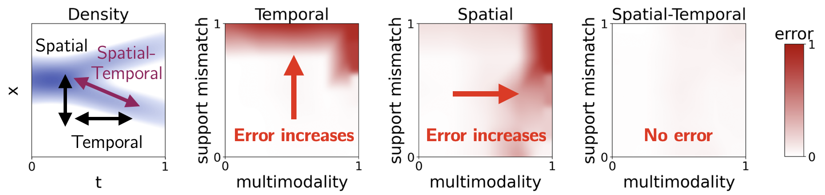
To analyze these failures, we study the ability of a model to relate the log-density of two points. For any two points, \((x,t)\) and \((x',t')\), we decompose the difference into spatial and/or temporal differences that need to be learnt by the model. This viewpoint captures both local properties (e.g., mode geometry for nearby points) and global properties (e.g., relative mode weights for distant points). Crucially, we will show that purely spatial or temporal decompositions inevitably require evaluating \(p(x,t)\) in low-density regions, where samples are scarce and estimation is therefore worse. Figure 1 empirically validates these claims to hold even for a bivariate density.
3.0.0.2 Spatial differences struggle with multimodality.
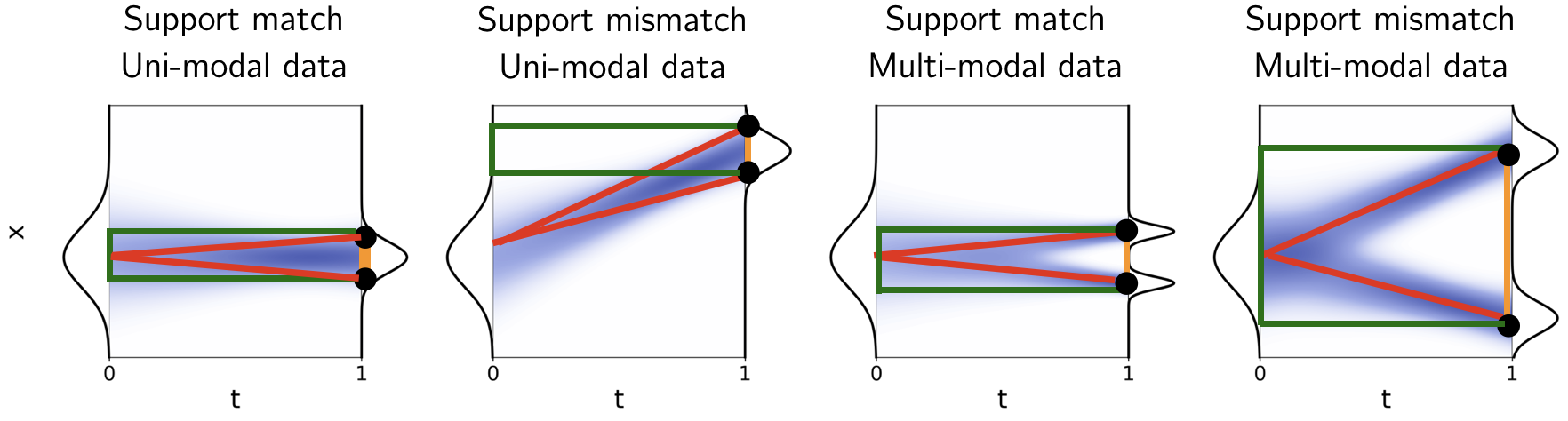
Spatial methods learn \(p_\theta(x,t)\) via differences in \(x\). Using our heuristic, we decompose the log-density difference between \(x\) and \(y\) as \[\begin{align} \log p(x,1)-\log p(y,1) =\sum_{i=0}^{K-1}\!\log p(x_{i+1},1)-\log p(x_i,1). \end{align}\] When \(p_1\) is multimodal (Figure 2, two right panels), these spatial differences in orange necessarily traverse low-density regions (white). Since such regions are poorly sampled, the corresponding spatial differences are poorly estimated. As a result, spatial methods—including energy-based diffusion models—struggle to capture global structure such as mode weights [27].
3.0.0.3 Temporal differences suffer from support mismatch.
Temporal methods learn \(p_\theta(x,t)\) via differences in \(t\). A simple algorithm, which we term tNCE, works by sampling \(t\) and \(t'\), and constructing binary classification problems; this was explored in [6], [29]. Again, using our heuristic, we decompose the log-density difference between \(x\) and \(y\) as \[\begin{align} \log p(x,1)-\log p(y,1) =\log p(x,0)-\log p(y,0)+\Delta, \end{align}\] where \(p(\cdot,0)\) is a known reference distribution, and \[\begin{align} \Delta =\sum_{i=0}^{K-1}\!\bigl(\log p(x,t_{i+1})-\log p(x,t_i)\bigr) -\sum_{i=0}^{K-1}\!\bigl(\log p(y,t_{i+1})-\log p(y,t_i)\bigr). \end{align}\] When the supports of \(p_0\) and \(p_1\) differ (Figure 2, second and fourth panels), these temporal differences in green traverse low-density regions in white. As before, this degrades estimation.
3.0.0.4 Spatiotemporal differences avoid both issues.
We now consider a joint discretization in space and time. Let \(\{(x_i,y_i,t_i)\}_{i=0}^K\) with \(x_i,y_i \sim p_{t_i}\). Then \[\log p(x,1)-\log p(y,1) =\log p(x_0,0)-\log p(y_0,0)+\Delta,\] where \(\Delta =\sum_{i=0}^{K-1}\!\bigl(\log p(x_{i+1},t_{i+1})-\log p(x_i,t_i)\bigr) -\sum_{i=0}^{K-1}\!\bigl(\log p(y_{i+1},t_{i+1})-\log p(y_i,t_i)\bigr).\)
As illustrated in Figure 2, these spatiotemporal differences in red can be chosen to remain within high-density regions in blue. Since such regions are well sampled, the corresponding spatiotemporal differences are accurately estimated.
This observation may explain the success of recent spatiotemporal methods [5]–[7], [28], [29], as they simultaneously address multimodality and support mismatch. We empirically validate this conjecture in Figure 1. This motivates the following unifying framework for spatiotemporal methods.
4 Learning the energy by spatiotemporal differences↩︎
In this section, we introduce a framework for estimating the parameters of an energy-based model by learning its variation jointly in data space and time. Our approach reduces to a single binary classification problem that unifies many popular methods [6], [7], [9], [10], [12]–[14], [17], [18], [20], [29]; see Table 5.
4.0.0.1 Spatiotemporal Noise-Contrastive Estimation (stNCE)
We propose to learn the energy by estimating its spatiotemporal differences, \(E(x’, t’) - E(x, t)\), by solving a binary classification task. We call this approach Spatiotemporal Noise-Contrastive Estimation (stNCE). First, generate data \((x, t, x', t')\) from two classes \(A\) and \(B\) \[\begin{align} p_A(x, t, x', t') = p_d(x, t) p_n(x', t' | x, t), \quad p_B(x, t, x', t') = p_d(x', t') p_n(x', t' | x, t). \end{align}\] To generate data from class \(A\), first sample a data point and its corruption level \((x, t)\) following Eq. 1 , and then perturb them into \((x', t')\) using a perturbation kernel \(p_n\) that is chosen by the user. Switching the positions of \((x, t)\) and \((x', t')\) in the tuple yields data from class \(B\). Efficient strategies for sampling \((x,t,x',t')\) are discussed in Appendix 10.1. Then, minimizing the logistic loss yields the optimal classifier \[\label{eq:stnce95classifier} F(x, t, x', t') = E(x',t')\!-\!E(x,t) +\!\log Z(t')\!-\!\log Z(t) +\!\log p_n(x',t'\mid x,t)\!-\!\log p_n(x,t\mid x',t'),\tag{3}\] which equals the spatiotemporal energy difference up to known terms. In practice, we parameterize \(E(x,t)\) and \(\log Z(t)\) using neural networks and learn them jointly. Note that this can be viewed as the CNCE from Section 2 but on the augmented space \((x, t)\), which we use to establish Theorem 2.
4.0.0.2 Statistical guarantees.
We next present statistical guarantees on the stNCE estimator: it is consistent and we can quantify its sample-efficiency.
Theorem 1 (Non-parametric consistency). Let \(p_\theta(x,t) = \exp(-E_\theta(x,t))/Z_\theta(t)\) be a parametric model, and suppose the data is generated with parameter \(\theta^*\). Then the stNCE estimator \(\hat{\theta}\), obtained by minimizing the empirical logistic loss with \(N\) samples, leads to a pointwise consistent estimator: \[\begin{align} p_{\hat{\theta}} \to p_{\theta^*} \quad \text{as } N \to \infty. \end{align}\]
We prove this in Appendix 8.2, and next characterize the estimator’s asymptotic sample efficiency.
Theorem 2 (Sample efficiency). (Based on [27]) Let \[\begin{align} F_\theta(x,t,x',t') = \log p_\theta(x,t) - \log p_\theta(x',t') + \log p_n(x',t'\mid x,t) - \log p_n(x,t\mid x',t'). \end{align}\] Then the estimator satisfies \[\|\hat{\theta} - \theta^*\|^2 = \frac{1}{N_d}\,\mathrm{Tr}\!\bigl(C_1^{-1} C_2 C_1^{-1}\bigr) + o\!\left(\frac{1}{N_d}\right),\] with the following, where expectations are taken under \(p_d(x,t)p_n(x',t'\mid x,t)\): \[\begin{align} C_1 = \mathbb{E}\!\left[ \nabla_\theta F_\theta \nabla_\theta F_\theta^\top \,\sigma(-F_{\theta^*})\,\sigma(F_{\theta^*}) \right] ,\quad C_2 = \mathbb{E}\!\left[ \nabla_\theta F_\theta \nabla_\theta F_\theta^\top \,\sigma(-F_{\theta^*})^2 \right]. \end{align}\]
4.0.0.3 Design choices.
The main design choice is the perturbation kernel \(p_n\). While our stNCE estimator is consistent for any choice of \(p_n\), its sample efficiency depends critically on this choice. As shown in Table 5, specific choices recover many existing methods based on temporal differences [9], [13], [14], [17], spatial differences [10], [12], [19], and spatiotemporal differences [5]–[7], [29].
In principle, one could optimize the asymptotic variance expression with respect to \(p_n\). As is often the case, this is analytically difficult. Instead, we adopt an empirical approach and propose choices of \(p_n\) that are heuristically well suited to the problem.
5 Choices of perturbation kernels↩︎
In this section, we propose three choices for the perturbation kernels, called mixture, white, and forward-reverse. We argue that the first two are sample-efficient when the perturbation is “small enough", while the last is sample-efficient when a certain quantity called the”space score" is well-approximated. In both cases, the guiding principle is that the pairs \((x,t)\) and \((x', t')\) used to estimate energy difference should remain in the manifold of the target distribution \(p_d(x,t)\) that we wish to estimate; because one of them is sampled from \(p_d(x, t)\) and is therefore likely to be on the data manifold, the perturbation kernel \(p_n\) used to obtain the second should avoid mapping samples outside of the data manifold, see Figure 3. We explain that certain recent methods in the literature [5], [7] can be viewed as special cases or variants on these perturbation kernels.

5.0.0.1 Mixture kernel.
This kernel perturbs either \(x\) or \(t\): \[p_n(x',t'\mid x,t) = \tfrac{1}{2}\, p_n(t'\mid t)\,\delta_{x}(x') + \tfrac{1}{2}\, p_n(x'\mid x)\,\delta_{t}(t').\] We refer to this variant as stNCE-m. It recovers a mixture of tNCE and tCNCE objectives, as we show in Appendix 9.
5.0.0.2 White noise kernel.
This kernel perturbs both \(x\) and \(t\), with the perturbation in terms of \(x\) being isotropic Gaussian noise: \[p_n(x',t'\mid x,t) = \mathcal{N}(x'\mid x,\sigma^2 I)\,p(t'|t).\] We refer to the resulting algorithm as stNCE-w. The intuition is that sufficiently small perturbations keep \((x',t')\) in the data manifold of \(p_d\). In the limit \(\sigma \to 0\), this recovers Dual Score Matching [7], as we prove in Appendix 8.4.
The two previous methods suffer from the same pathology: under the scenario where the perturbation is non-vanishing, \((x',t')\) could naturally be generated off the high density region induced by \(p_{d}(x,t)\). The manifold hypothesis states that real world data often lies on a low dimensional Riemannian manifold, such that adding isotropic Gaussian noises often results in off-manifold samples. Furthermore, counter-intuitively, samples from Gaussian distribution concentrate near a sphere in high dimensions, resulting in non-smooth landscape even for noise-perturbed data. The same issues will affect tCNCE when used with a white noise kernel.
In contrast to the kernels above, the following kernel aims to stay within the manifold of \(p_d(x,t)\).
5.0.0.3 Forward-reverse kernel.
We propose perturbing \((x,t)\) along trajectories consistent with \(p_d(x,t)\): \[p_n(x',t'\mid x,t) = p_n(x'\mid x,t,t')\,p_{n}(t'|x).\] We first perturb \(t\) to \(t'\), then apply a kernel on \(x\): a noising step if \(t'<t\), and a denoising step if \(t'>t\). These kernels are Bayes inverses, as in diffusion-based methods [5], [35], [36].
An explicit construction based on the stochastic interpolant Eq. 1 is: \[\label{eq:forward-reverse-kernel}p_{n}(x'\mid x,t,t') = \begin{cases} \mathcal{N}\!\left(x'\middle| x/t,\; 1 - (1-t)^2/t^2 \right), & t'<t,\\[0.3em] \mathcal{N}\!\left( x'\middle| (t'/t)x + \tfrac{2(1-t)(t'-t)}{t}\,\nabla_x \log p_t(x),\; \tfrac{(t'-t)(t+t'-2tt')}{t^2} I \right), & t'>t. \end{cases}\tag{4}\]
The noising kernel (top) is tractable, while the denoising kernel, obtained using the exponential integrator formula [37], depends on
the space score \(\nabla_x \log p_t(x)\), which is typically unknown and is the key quantity that diffusion models approximate [34]. We approximate it using either: (i) oracle scores (when available), denoted as stNCE-o, or (ii) self scores, obtained from the current model, denoted as stNCE-s. The latter is reminiscent of
consistency models and flow maps [38], [39].We further
note that the recent RNE regularization [5] proposed to regularize energy-based diffusion models is related too, with the following differences: it uses
a squared loss instead of the logistic loss, and sampling is performed directly using the forward process without relying on the scores. However, unlike stNCE, which remains consistent for arbitrary kernels, e.g. the ones induced by
imperfect scores, and can be optimized independently, RNE depends heavily on the quality of the current score estimates: RNE loss based on inaccurate scores fail to remain consistent. Consequently, RNE mandates joint training with denoising score matching
loss or an oracle access to the ground truth socre, whereas stNCE could function as a standalone training objective.
5.0.0.4 Infinitesimal limit.
We now characterize the behavior of stNCE for certain infinitesimal perturbation kernels. Specifically, we study perturbation kernels that are transition probabilities along a trajectory of a Stochastic Differential Equation (SDE) as in Eq. 4 or of a Ordinary Differential Equation (ODE), assuming oracle access to the ground truth scores. We prove the following results in Appendix 8.3.
Proposition 3 (Transition probability of an SDE). Consider a stochastic interpolant as in Eq. 1 whose marginal laws \(p_t\) are simulated by the time-reversal of an SDE, \(\require{physics} \dd X_t = b(X_t, t) \dd t + g(t) \dd W_t\). Define the perturbation kernel to be the transition probability of that SDE. In the limit \(\Delta t \to 0\), stNCE recovers the space score matching loss with maximum-likelihood weighting [40]: \[\begin{align} \mathcal{L}_{\mathrm{stNCE}}(\theta) = 2\log 2 + \frac{\Delta t}{4}\, \mathbb{E}_{p_t}\!\left[ g(t)^2 \|\nabla_x \log p_t(x) - \nabla_x \log p_t^{\theta}(x)\|^2 \right] + o(\Delta t). \end{align}\]
Proposition 4 (Transition probability of an ODE). Consider a stochastic interpolant as in Eq. 1 whose marginal laws \(p_t\) are simulated by an ODE, \(\require{physics} \dd X_t = v(X_t) \dd t\). Define the perturbation kernel to be the transition probability of that ODE. Under this scenario, the transition kernels are Dirac deltas subject to Jacobian scalings. In the limit \(\Delta t \to 0\), stNCE recovers a loss for matching the trajectory-wise rate of change of the true and model log densities: \[\require{physics} \begin{align} \mathcal{L}_{\mathrm{stNCE}}(\theta) = 2\log 2 + \frac{\Delta t^2}{4}\, \mathbb{E}_{p_t}\!\left[ \| \dd_t \log p_t(x) - \dd_t \log p_t^\theta(x) \|^2 \right] + o(\Delta t^2). \end{align}\] where \(\require{physics} \dd_t \log p_t(x) := \partial_t \log p_t(x) + \nabla_{x} \log p_t(x) \cdot v_t(x)\).
6 Experiments↩︎
We empirically evaluate our framework for learning densities of synthetic data, images and molecules. In particular, we report results of the different variants of our Spatiotemporal Noise-Contrastive Estimation (stNCE-m, stNCE-w, stNCE-s, stNCE-o) that are detailed in Section 5. We also use another variant stNCE-s\(+\)DSM which combines stNCE-s with a space score matching loss: the former estimates spatiotemporal differences while the latter estimates infinitesimal spatial differences. See Appendix 10.4 for further details. Across datasets, our stNCE-s and variants are most promising: they are competitive with the state of the art.
6.1 Failure modes↩︎
Many methods for learning energy-based models, including denoising score matching used in diffusion models [4], [41], are typically evaluated on complex datasets. Yet, Figure 1 shows that they can already fail in a simple one-dimensional setting. This experiment highlights two key properties of the data distribution that drive these failures. First, multimodality increases the error of methods based on learning spatial differences. Second, a mismatch between the high-density regions (“supports”) of the data and reference distributions increases the error of methods based on learning temporal differences. Methods based on learning spatiotemporal difference are robust to both sources of error. Details on the simulations are provided in Appendix 11.1.
6.2 Gaussian mixtures↩︎
6.2.0.1 Setup and dataset
Image data are high-dimensional and sparse. To emulate these properties, we build a Gaussian mixture from the MNIST dataset [42] by sampling \(100\) images (\(10\) per digit class) and using them as centroids with diagonal covariance \(0.01 I\). This synthetic yet realistic distribution exhibits the two pathologies identified in Section 3: strong multimodality and minimal overlap with a standard Gaussian reference distribution due to its thin support. We therefore expect purely spatial and purely temporal methods to struggle, while spatio-temporal methods with density-aware kernels should perform well, which is confirmed in Table 1.
6.2.0.2 Evaluation
We use the following metrics to evaluate if model and ground-truth density agree. They are computed as averages over data samples and to the model density and also the data density (which is usually unavailable, but we know it for toy experiments). When we have access to both the ground truth data density and the sampling mechanism that generates samples from it, we can estimate the log constant of the model density at the time corresponding to clean data using importance sampling, denoted as \(\widehat{\log Z_1}\), and evaluate the model density normalized using \(\widehat{\log Z_1}\). \[\begin{align} \mathrm{MSE} &:= \mathbb{E}_{x \sim p_d(\cdot \mid 1)} \!\left[ \bigl( \log p_d(x \mid 1) - \log p_\theta(x \mid 1) \bigr)^2 \right], \\ \mathrm{Ratio} &:= \mathbb{E}_{x,x' \sim p_d(\cdot \mid 1)^{\otimes 2}} \!\left[ \Bigl( \log p_d(x \mid 1) - \log p_d(x' \mid 1) - \log p_\theta(x \mid 1) + \log p_\theta(x' \mid 1) \Bigr)^2 \right], \\ \mathrm{NormMSE} &:= \mathbb{E}_{x \sim p_d(\cdot \mid 1)} \!\left[ \bigl( \log p_d(x \mid 1) - \log p_\theta(x \mid 1) + \widehat{\log Z_1} \bigr)^2 \right], \\ \mathrm{NormNLL} &:= \mathbb{E}_{x \sim p_d(\cdot \mid 1)} \!\left[ - \log p_\theta(x \mid 1) + \widehat{\log Z_1} \right]. \end{align}\] The first is the squared error between the data and model log densities. The second is the squared error between spatial differences of the data and model log densities — this metric is well-suited for evaluating unnormalized densities given that it does not depend on normalizing constants. The third and the fourth evaluate how good the model is as an unnormalized EBM, though naturally depends on the accuracy of the estimated \(\widehat{\log Z_1}\).
6.2.0.3 Results
Among spatiotemporal methods, we study two perturbation kernels: white noise and the forward–reverse kernel from Section 5. Results with white noise match the intuition of Figure 3: finite Gaussian perturbations (stNCE-w) perform poorly because they push samples off the data manifold, whereas infinitesimal perturbations (Dual SM [7]) preserve proximity to the manifold and yield accurate estimates, albeit at higher computational cost due to double differentiation through the network. Results for the forward–reverse kernel further support this interpretation. Even with finite corruption, stNCE-s remains competitive because it stays close to the data manifold. By contrast, as discussed in Section 3, RNE [5] is consistent only when given access to the true scores \(\nabla_{x_t} \log p_t(x_t)\) (RNE-o), which are unavailable in practice; using estimated scores (RNE-s) can lead to substantial degradation. Our implementation of stNCE-m naively adds up tNCE loss and tCNCE loss, leading to slower running time, as indicated using \(^*\); this also applies to later experiments.
Overall, stNCE-s provides a favorable trade-off between accuracy and speed, and is the only NCE-based method that successfully learns this challenging Gaussian mixture.
| Category | Method | MSE \(\downarrow\) | Ratio \(\downarrow\) | NormMSE \(\downarrow\) | NormNLL \(\downarrow\) | Time \(\downarrow\) |
|---|---|---|---|---|---|---|
| Temporal | \(2{\times}10^{5} \pm 4{\times}10^{3}\) | 958.11 \(\pm\) 131.63 | \(7{\times}10^{3} \pm 1{\times}10^{3}\) | -606.76 \(\pm\) 7.83 | 0.39 | |
| \(3{\times}10^{5} \pm 1{\times}10^{5}\) | \(1{\times}10^{3} \pm 608.53\) | \(8{\times}10^{3} \pm 2{\times}10^{3}\) | -602.92 \(\pm\) 9.59 | 0.68 | ||
| Spatial | \(2{\times}10^{5} \pm 5{\times}10^{4}\) | \(3{\times}10^{3} \pm 584.77\) | \(9{\times}10^{3} \pm 2{\times}10^{3}\) | -598.73 \(\pm\) 7.82 | 0.4 | |
| \(1{\times}10^{7} \pm 9{\times}10^{5}\) | \(1{\times}10^{4} \pm 4{\times}10^{3}\) | \(3{\times}10^{4} \pm 1{\times}10^{4}\) | -535.54 \(\pm\) 28.81 | 0.7 | ||
| Spatio- temporal | \(3{\times}10^{4} \pm 4{\times}10^{3}\) | 600.77 \(\pm\) 276.83 | \(2{\times}10^{3} \pm 846.83\) | -644.8 \(\pm\) 8.51 | 0.45\(^{*}\) | |
| \(2{\times}10^{4} \pm 1{\times}10^{3}\) | 412.73 \(\pm\) 148.16 | \(2{\times}10^{3} \pm 458.16\) | -652.43 \(\pm\) 5.22 | 0.4 | ||
| 121.6 \(\pm\) 11.77 | 28.31 \(\pm\) 1.93 | 65.02 \(\pm\) 7.67 | -680.99 \(\pm\) 0.53 | 0.36 | ||
| \(3{\times}10^{6} \pm 1{\times}10^{6}\) | \(3{\times}10^{3} \pm 945.15\) | \(2{\times}10^{4} \pm 702.98\) | -570.51 \(\pm\) 1.09 | 0.44 | ||
| 42.16 \(\pm\) 7.11 | 17.82 \(\pm\) 1.02 | 26.04 \(\pm\) 2.82 | -683.96 \(\pm\) 0.33 | 0.7 | ||
| Oracle | 148.61 \(\pm\) 17.09 | 40.25 \(\pm\) 2.35 | 141.75 \(\pm\) 3.61 | -677.07 \(\pm\) 0.12 | 0.32 | |
| 18.57 \(\pm\) 1.46 | 7.88 \(\pm\) 0.19 | 9.41 \(\pm\) 0.61 | -685.75 \(\pm\) 0.09 | 0.4 |
3pt
6.3 Images↩︎
In this section, we follow previous related works [7], [17] in reporting the Negative Log-Likelihood (NLL) in bits per dimension, for image datasets \[\begin{align} \mathrm{NLL}_{\mathrm{bpd}} := \frac{ -\mathbb{E}_{x \sim p_d(\cdot \mid 1)} \!\left[ \log p_\theta(x \mid 1) \right] }{ D \log 2 }, \end{align}\] where \(D\) is the data dimension (e.g. the number of pixels times channels for images). Note that we do not use the NormNLL for two reasons. First, related works [7] do not use it and we wish to replicate a fair comparison. Second, the idea behind NormNLL is to correct the approximate normalization of the model using a sepearate estimate of the normalizing constant. In Section 6.2, we could obtain a precise estimate because we knew the ground-truth distribution of the dataset. Here, we do not know the ground-truth distribution and the standard way of estimate the normalizing constant is using AIS which in our preliminary experiments and in related literature [17] was very high-variance on image datasets.
6.3.0.1 MNIST
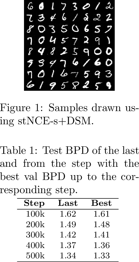
We next train the different algorithms to learn the data density of images from the MNIST dataset of handwritten digits [42]. Results are shown in Table ¿tbl:table:mnist?: our stNCE-s is still the best variant among NCE algorithms and reaches state-of-the-art performance while being fast to train. Here our algorithms were trained for \(100,000\) steps; we verify in Table [tbl:mnist-tstnce-long] that stNCE-s continues to improve when optimized longer. Alternatively, on can use our stNCE-s\(+\)DSM which reaches state-of-the-art results, by jointly estimate the spatial scores of the density. Samples drawn from our model in Figure [tbl:fig:mnist95samples] look realistic.

6.3.0.2 ImageNet
| Method | Anti-aliasing | Augmentation | Discreteness | Type | Single NFE | NLL |
|---|---|---|---|---|---|---|
| Glow [43] | None | Continuous | Normalized | 3.81 | ||
| PixelCNN [44] | None | Discrete | Normalized | 3.57 | ||
| I-DDPM [45] | None | Continuous | Upper bound | 3.54 | ||
| VDM [46] | None | Discrete | Upper bound | 3.40 | ||
| FM [30] | None | Uniform* | Normalized | 3.31 | ||
| NFDM [47] | Horizontal flips | Uniform* | Normalized | 3.20 | ||
| TarFlow [48] | Horizontal flips | Uniform | Normalized | 2.99 | ||
| Dual SM [7] | Horizontal flips | Continuous | Estimate | 3.36 | ||
| Ours () | Horizontal flips | Continuous | Estimate | 2.94 |
![Figure 4: ImageNet test set images with the highest densities (left) and the lowest densities (right) as identified using our model. Higher likelihood images appear to have higher frequencies manifested by sharper contours and shapes, while lower likelihood images appear to have lower frequencies in the form of regular geometric patterns. This is consistent with the literature [7].](/article/2605.26850/image/imagenet/eval2_extreme_log_densities.png "fig:")
As a comparison against the state-of-the-art in larger scale, we repeat the experiment on ImageNet64 [49]. In Table 2, we can see that our stNCE-s\(+\)DSM is competitive with Flow Matching [30] and outperforms approaches such Dual Score-Matching [7], which similarly models the data density as an energy-based model. We verify in Figure 4 that our learnt model assigns high probability to sharper images and lower probability to blurrier images.
6.4 Molecules↩︎
6.4.0.1 Setup and datasets
We wish to model a target distribution (a.k.a. equilibrium distribution) over configurations of a molecule. Concretely, each data point in that space is the collection of three-dimensional positions of the atoms, or rather groups of atoms called chains, that make up the molecule. In our experiments, we consider two “coarse-grained" molecular systems: Alanine dipeptide (ALDP) and Chignolin. Specifically, the ALDP is represented by \(5\) chains and Chignolin by \(10\) chains; because each chain has three-dimensional spatial coordinates, this leads to \(15\)-dimensional and \(30\)-dimensional data, respectively. Data points in”high probability" regions correspond to likely spatial configurations of the atoms. In practice, we have access energy and score function (a.k.a. force field) of the target distribution via physics, but they are expensive to evaluate as they require solving a PDE. To avoid evaluating them for every new data point, there are two prevailing approaches in the literature.
The first approach is Machine Learning Force Fields (MLFFs), which regress a neural network against the energy and score functions on some finite grid of data points [50], [51]. The second approach which we follow here is Energy-Based Models (EBMs) that learn a neural network that matches the energy of the target distribution. Such models are trained on a dataset of samples that approximately follow the target distribution. To form such a dataset, a sampling process such as Langevin Dynamics (a.k.a. Molecular Dynamics), which requires evaluating the target energy and score functions, is run long enough so that the final samples are approximately i.i.d. samples from the target distribution. In practice, we use the datasets provided [28] and [52], following the same architecture and parameterization as [28].
6.4.0.2 Methods
We compare stNCE to another spatiotemporal method from [28] based on the Fokker-Planck Equation (FPE). That method consists in learning spatial differences of the energy using a loss we detail in Appendix 9.11, and temporal differences of the energy by minimizing a PINN loss that effectively forces the energy to follow a certain Partial Differential Equation. Although technically sound, FPE is computationally expensive because it requires optimizing through the second-order derivative of the energy network. Even with the estimator proposed by [28] to bypass explicit second-order derivatives, the FPE approach remains costly due to the multiple additional network evaluations required per loss calculation. In contrast, stNCE is fundamentally more efficient to optimize.
6.4.0.3 Evaluation
To evaluate the quality of the estimated model of the data \(p_{\theta}(x | 1)\), we use the following metrics from [28]. The Potential Mean Field (PMF) is just the mean-squared error between the model energy and true energy, comptued over data samples. The Jensen-Shannon Divergence (JSD) is a statistical divergence between the ground truth and model densities. \[\begin{align} \mathrm{PMF}(\theta) &= \mathbb{E}_{x \sim p_d(\cdot | 1)} \big[ \big( E(x, 1) - E_{\theta}(x, 1) \big)^2 \big] \\ \mathrm{JSD}(\theta) &= \log 2 + \frac{1}{2} \mathbb{E}_{x \sim p_d(\cdot \mid 1)} \bigg[ \log \frac{p_d(x \mid 1)}{p_d(x \mid 1)+p_\theta(x \mid 1)} \bigg] + \frac{1}{2} \mathbb{E}_{x \sim p_\theta(\cdot \mid 1)} \bigg[ \log \frac{p_\theta(x \mid 1)}{p_d(x \mid 1)+p_\theta(x \mid 1)} \bigg]. \end{align}\] In practice, these metrics are not computed over the full data space but on a physically meaningful \(2\)-dimensional subspace: the torsional angles for ALDP, and the principle directions of multi-modality obtained by Time-lagged Independent Component Analysis (TICA) [53], [54] for Chignolin.
To compute these metrics, we proceed as follows. First, we start with samples on the full data samples: ground-truth samples \(x \sim p_d(x | 1)\) are from the the dataset and the samples from our model \(x \sim p_{\theta}(x | 1)\) are obtained by running two score-based samplers, the Langevin sampler which uses the final score \(\nabla \log p_{\theta}(x | 1)\) [55] and the diffusion sampler which uses the intermediate scores \(\nabla \log p_{\theta}(x | t)\) [34]. Second, we project the ground-truth and model samples onto the \(2\)-dimensional subspace. Third, we compute histogram-based density estimates of the corresponding \(2\)-dimensional ground-truth and model distributions. Finally, we compute an empirical version of the above metrics, where the expectations are replaced by a finite-sample average.
6.4.0.4 Results
[tab:aldp-full-results,tbl:chignolin-results] report the Jensen-Shannon (JS) divergence and Potential
of Mean Force (PMF) metrics (lower is better). They show that stNCE effectively generates these consistent samples and achieves performance comparable to FPE. On the other hand, training jointly with DSM consistently improves performance while introducing
only marginal computational overhead. In fact, the estimated training time (in GPU hours of a single NVDIA A100) of different methods is as follows: DSM is the fastest method (8.71) but achieves lower performance. stNCE-s(16.87) is the next
fastest and adding DSM slightly increases its runtime (18.85) while still being \(2.5\)-fold faster than FPE (49.57).
| Method | IID JS \(\downarrow\) | Langevin JS \(\downarrow\) | IID PMF \(\downarrow\) | Langevin PMF \(\downarrow\) |
|---|---|---|---|---|
| \(0.0093 \pm 0.0001\) | \(0.0111 \pm 0.0003\) | \(0.095 \pm 0.001\) | \(0.119 \pm 0.003\) | |
| \(0.0063 \pm 0.0000\) | \(0.0065 \pm 0.0001\) | \(0.063 \pm 0.002\) | \(0.066 \pm 0.003\) | |
| \(0.0098 \pm 0.0002\) | \(0.0111 \pm 0.0001\) | \(0.106 \pm 0.004\) | \(0.139 \pm 0.001\) | |
| \(0.0072 \pm 0.0000\) | \(0.0082 \pm 0.0002\) | \(0.076 \pm 0.002\) | \(0.088 \pm 0.005\) | |
| FPE [28] | \(0.0082 \pm 0.0002\) | \(0.0090 \pm 0.0006\) | \(0.098 \pm 0.003\) | \(0.104 \pm 0.004\) |
| Method | IID JS \(\downarrow\) | Langevin JS \(\downarrow\) | IID PMF \(\downarrow\) | Langevin PMF \(\downarrow\) |
|---|---|---|---|---|
| \(0.0593 \pm 0.0001\) | \(0.2420 \pm 0.0020\) | \(0.654 \pm 0.001\) | \(3.143 \pm 0.031\) | |
| \(0.0073 \pm 0.0019\) | \(0.0181 \pm 0.0055\) | \(0.060 \pm 0.015\) | \(0.162 \pm 0.053\) | |
| \(0.0097 \pm 0.0000\) | \(0.0199 \pm 0.0015\) | \(0.083 \pm 0.000\) | \(0.170 \pm 0.014\) | |
| \(0.0074 \pm 0.0001\) | \(0.0082 \pm 0.0006\) | \(0.059 \pm 0.001\) | \(0.065 \pm 0.005\) | |
| FPE [28] | \(0.0048 \pm 0.0001\) | \(0.0050 \pm 0.0001\) | \(0.037 \pm 0.000\) | \(0.039 \pm 0.001\) |
7 Discussion↩︎
7.0.0.1 Compute burden of the likelihood: training-time versus inference-time
This work highlights how the literature of learning energy-based models falls within three families of learning objectives: temporal, spatial, and spatiotemporal. Another axis for organizing the literature is two parameterizations of the energy-based model differences, both enabling likelihood estimation but differing primarily in when the computational burden is incurred.
A first class defers this cost to inference time by integrating learned quantities, including temporal methods based on \(\partial_t \log p_t(x)\) [14], [17], [56], spatial methods based on \(\nabla \log p_t(x)\), and spatio-temporal approaches integrating \(\frac{\mathrm{d}}{\mathrm{d}t} \log p_t(x_t)\), such as continuous normalizing flows [57] and path-wise formulations [14]. These methods are relatively easy to train, as they avoid higher-order differentiation, but incur significant inference-time cost due to numerical integration, although recent works look into learn to integrate in few steps [8], [39], [58].
A second class instead parameterizes these differences directly with an energy-based model, enabling one-step likelihood evaluation. This includes temporal methods such as NCE [9], spatial methods such as (denoising) score matching [12], [20], and recent spatio-temporal approaches, including ours [5]–[7], [28], [29]. These methods yield cheap inference—often a single network evaluation—but are harder to train, e.g., due to higher-order autodiff.
Overall, these approaches trade training-time for inference-time compute. We focus on the latter regime, favoring expensive training for efficient inference. A systematic study of this trade-off is left for future work.
7.0.0.2 Limitations and future directions
While models trained using NCE loss functions can recover the ground truth energies accurately, the scores may not be learned well when comparing to the score matching variants. Future work could explore better samplers for models trained with NCE losses that either do not rely on gradient information or could better handle noisy gradients.
7.0.0.3
In conclusion, we show that despite their diversity, most energy-based model estimation methods fall into three categories: spatial, temporal, and spatiotemporal. We identify fundamental failure modes of purely spatial and temporal approaches, and show how spatiotemporal methods overcome them. Our unified binary classification framework recovers many existing methods and yields new objectives with near state-of-the-art performance across synthetic, image, and molecular data.
Acknowledgements and Disclosure of Funding↩︎
The authors wish to acknowledge Florentin Guth for interesting discussions on Dual Score Matching [7].
Hanlin Yu and Arto Klami acknowledge the research environment provided by ELLIS Institute Finland, and were supported by the Research Council of Finland Flagship programme: Finnish Center for Artificial Intelligence FCAI. RuiKang OuYang acknowledges the UK Engineering and Physical Sciences Research Council (EPSRC) grant EP/L016516/1 for the University of Cambridge Centre for Doctoral Training, the Cambridge Centre for Analysis. Michael U. Gutmann was supported in part by Gen AI - the AI Hub for Generative Models, funded by EPSRC (EP/Y028805/1).
The authors wish to acknowledge CSC - IT Center for Science, Finland, for computational resources, and acknowledge CSC - IT Center for Science, Finland for awarding this project access to the LUMI supercomputer, owned by the EuroHPC Joint Undertaking, hosted by CSC(Finland) and the LUMI consortium through CSC - IT Center for Science, Finland.
Appendix↩︎
The appendix is organized as follows.
8 Theoretical results↩︎
In this section, we prove the consistency of the estimator obtained by minimizing the empirical stNCE loss. We also derive the simplified expressions of stNCE loss under specific perturbation kernels.
8.1 Useful lemma on the logistic loss↩︎
The following are useful lemma on how to rewrite the logistic classification loss.
Lemma 1 (Logistic loss as a Bregman divergence). Consider the logistic loss \[\begin{align} \mathcal{L}_{\mathrm{logistic}}(F) = - \mathbb{E}_{x \sim p_{A}} \left[ \log \sigma(F(x)) \right] - \mathbb{E}_{x \sim p_{B}} \left[ \log (1 - \sigma(F(x))) \right], \end{align}\] which is minimized by \[F^{*}(x) = \log p_A(x) - \log p_B(x).\] Then, up to an additive constant independent of \(F\), the logistic loss can be written as a Bregman divergence between \(e^{F^*}\) and \(e^F\).
Proof. This is inspired by [59], [60].
Let \(\Phi(u) = u \log u - (1+u)\log(1+u)\). Consider the pointwise Bregman divergence \[\begin{align} D_{\Phi}\big(e^{F^*(x)}, e^{F(x)}\big) = \Phi\big(e^{F^*(x)}\big) - \Phi\big(e^{F(x)}\big) - \Phi'\big(e^{F(x)}\big)\big(e^{F^*(x)} - e^{F(x)}\big). \end{align}\] Integrating against \(p_B(x)\,dx\) yields a divergence between functions: \[\begin{align} D_{\Phi}\big(e^{F^*}, e^{F}\big) = \int D_{\Phi}\big(e^{F^*(x)}, e^{F(x)}\big)\, p_B(x)\,dx. \end{align}\] Substituting \(F^*(x) = \log p_A(x) - \log p_B(x)\), a straightforward calculation shows \[\begin{align} D_{\Phi}\big(e^{F^*}, e^{F}\big) = \mathcal{L}_{\mathrm{logistic}}(F) - \mathcal{L}_{\mathrm{logistic}}(F^*), \end{align}\] which proves the claim. ◻
Lemma 2 (Logistic loss simplified when the model is near zero). Consider the logistic loss \[\begin{align} \mathcal{L}(F_{\theta}) &:= - \mathbb{E}_{p^{+}(x)} \bigl[ \log \sigma(F_{\theta}(x)) \bigr] - \mathbb{E}_{p^{-}(x)} \bigl[ \log \bigl( 1 - \sigma(F_{\theta}(x)) \bigr) \bigr]. \end{align}\] If \(F_\theta(x)\) is close to zero, then \[\begin{align} \mathcal{L}(F_\theta) &= \mathcal{L}(0) - \frac{1}{2} \mathbb{E}_{p^{+}(x)-p^{-}(x)} \left[ F_\theta(x) \right] + \frac{1}{8} \mathbb{E}_{p^{+}(x)+p^{-}(x)} \left[ F_\theta(x)^2 \right] + \mathbb{E}_{p^{+}(x)+p^{-}(x)} \left[ o(F_\theta(x)^2) \right]. \end{align}\]
Proof. For fixed \(x\), define the pointwise loss \[\begin{align} \ell(F_{\theta}) &:= - p^{+}\log \sigma(F_{\theta}) - p^{-}\log \bigl(1-\sigma(F_{\theta})\bigr). \end{align}\] A second-order Taylor expansion around \(F_{\theta}=0\) gives \[\begin{align} \ell(F_\theta) &= \ell(0) - \frac{1}{2} \bigl(p^{+}-p^{-}\bigr) F_\theta + \frac{1}{8} \bigl(p^{+}+p^{-}\bigr) F_\theta^2 + \bigl(p^{+}+p^{-}\bigr) o(F_\theta^2). \end{align}\] Integrating over \(x\) yields the result. ◻
8.2 Non-parametric consistency (Theorem 1)↩︎
Recall that the stNCE population loss is the logistic classification objective \[\begin{align} \mathcal{L}_{\mathrm{stNCE}}(F) = - \mathbb{E}_{x \sim p_{A}} \big[ \log \sigma(F(x)) \big] - \mathbb{E}_{x \sim p_{B}} \big[ \log (1 - \sigma(F(x))) \big]. \end{align}\] By Lemma 1, this can be written (up to an additive constant) as \[\begin{align} \mathcal{L}_{\mathrm{stNCE}}(F) = D_{\Phi}\big(e^{F^*}, e^{F}\big) + \mathrm{const}. \end{align}\] Hence any minimizer \(F^{\theta_{\min}}\) satisfies \[F^{\theta_{\min}} = F^*.\]
Using the definition of the stNCE classifier Eq. 3 , this yields, for all \((x,t)\) and \((x',t')\) in the support, \[\begin{align} \log p_{\theta_{\min}}(x \mid t) - \log p_{\theta_{\min}}(x' \mid t') = \log p_d(x \mid t) - \log p_d(x' \mid t'). \end{align}\] Therefore, \[\begin{align} \log p_{\theta_{\min}}(x \mid t) = \log p_d(x \mid t) + C, \end{align}\] where \(C\) does not depend on \((x,t)\). Enforcing the constraint \(p_\theta(x \mid t=0) = p_0(x)\) fixes \(C\), yielding \[\begin{align} p_{\theta_{\min}}(x \mid t) = p_d(x \mid t). \end{align}\]
This establishes non-parametric consistency. If the model is identifiable, we further obtain parametric Fisher consistency, i.e., \[\theta_{\min} = \theta^*.\]
8.3 Forward-reverse kernel: Infinitesimal Limit (Propositions 3 and Proposition 4)↩︎
8.3.0.1 Simplifying the loss around zero
Let \[\begin{align} p_+(x,t,x',t') &:= p_d(x,t)p_n(x',t' \mid x,t), \\ p_-(x,t,x',t') &:= p_d(x',t')p_n(x,t \mid x',t'). \end{align}\] The logistic loss used in stNCE is \[\mathcal{L}(F_{\theta}) = -\mathbb{E}_{p_+(x, t, x', t')} [\log \sigma(F_{\theta}(x, t, x', t'))] -\mathbb{E}_{p_-(x, t, x', t')} [\log (1 - \sigma(F_{\theta}(x, t, x', t')))] .\] Using Lemma 2, we have, whenever \(F_\theta\) is close to zero, \[\begin{align} \mathcal{L}(F_\theta) &= \mathcal{L}(0) - \frac{1}{2} \mathbb{E}_{p_+ - p_-} \left[ F_\theta \right] + \frac{1}{8} \mathbb{E}_{p_+ + p_-} \left[ F_\theta^2 \right] + \mathbb{E}_{p_+ + p_-} \left[ o(F_\theta^2) \right]. \end{align}\] In contrast with the expansion around the optimum, this expansion generally contains a linear term. However, this term vanishes in the forward-reverse case considered below.
8.3.0.2 Plugging in the forward-reverse kernel
Recall that the forward-reverse kernel satisfies \[\begin{align} p_d(x,t)p_n(x',t'\mid x,t) = p_d(x',t')p_n(x,t\mid x',t'), \end{align}\] due to the Bayes rule. Equivalently, \[\begin{align} p_+(x,t,x',t') = p_-(x,t,x',t'). \end{align}\] Therefore, the linear term vanishes: \[\begin{align} \mathbb{E}_{p_+ - p_-} \left[ F_\theta \right] = 0. \end{align}\] Moreover, by taking logs in the forward-reverse identity, \[\begin{align} \log p_n(x',t'\mid x,t) - \log p_n(x,t\mid x',t') = \log p_d(x',t') - \log p_d(x,t). \end{align}\] Hence \[\begin{align} F_\theta(x,t,x',t') &= \log p_\theta(x,t) - \log p_\theta(x',t') \\ &\quad+ \log p_n(x',t'\mid x,t) - \log p_n(x,t\mid x',t') \\ &= \log p_\theta(x,t) - \log p_\theta(x',t') + \log p_d(x',t') - \log p_d(x,t) \\ &= \bigl( \log p_d(x',t') - \log p_\theta(x',t') \bigr) - \bigl( \log p_d(x,t) - \log p_\theta(x,t) \bigr). \end{align}\] Defining \[\begin{align} e_\theta(x,t) := \log p_d(x,t)-\log p_\theta(x,t), \end{align}\] we obtain \[\begin{align} F_\theta(x,t,x',t') = e_\theta(x',t')-e_\theta(x,t). \end{align}\] Since \(p_+=p_-=p_d(x,t)p_n(x',t'\mid x,t)\), the expansion becomes \[\begin{align} \mathcal{L}(F_\theta) &= \mathcal{L}(0) + \frac{1}{4} \mathbb{E}_{p_d(x,t)p_n(x',t'\mid x,t)} \left[ \bigl( e_\theta(x',t')-e_\theta(x,t) \bigr)^2 \right] \\ &\quad+ \mathbb{E}_{p_d(x,t)p_n(x',t'\mid x,t)} \left[ o\!\left( \bigl( e_\theta(x',t')-e_\theta(x,t) \bigr)^2 \right) \right]. \end{align}\] This expansion is valid when \(F_\theta\) is close to zero. In the infinitesimal-time regime, this follows from the fact that \((x',t')\) is close to \((x,t)\).
8.3.0.3 Case of the SDE
Assume that \(x_t\) follows the SDE \[\require{physics} \begin{align} \dd x_t = b(x_t,t)\dd t + g(t)\dd W_t. \end{align}\] Let \(t'=t+\Delta t\). Conditional on \((x_t,t)=(x,t)\), the next point satisfies \[\begin{align} x' = x + b(x,t)\Delta t + g(t)\Delta W + R_t, \qquad \Delta W\sim \mathcal{N}(0,\Delta t\,I), \end{align}\] where \[\begin{align} R_t = \int_t^{t+\Delta t} \bigl( b(x_s,s)-b(x,t) \bigr)\,ds + \int_t^{t+\Delta t} \bigl( g(s)-g(t) \bigr)\,dW_s . \end{align}\] Therefore, the expectation with respect to the transition kernel \(p_n(x',t'\mid x,t)\) may be written as an expectation with respect to the Brownian increment \(\Delta W\).
By Itô’s lemma, \[\begin{align} e_\theta(x',t')-e_\theta(x,t) &= \partial_t e_\theta(x,t)\Delta t + \nabla_x e_\theta(x,t)^\top b(x,t)\Delta t \\ &\quad+ g(t) \nabla_x e_\theta(x,t)^\top \Delta W + \frac{1}{2} g(t)^2 \operatorname{Tr} \left( \nabla_x^2 e_\theta(x,t) \right) \Delta t + o(\Delta t). \end{align}\] Since \(\Delta W=O(\sqrt{\Delta t})\), the leading term is \[\begin{align} e_\theta(x',t')-e_\theta(x,t) = g(t) \nabla_x e_\theta(x,t)^\top \Delta W + O(\Delta t). \end{align}\] Thus, conditionally on \((x,t)\), \[\begin{align} \mathbb{E}_{\Delta W} \left[ \bigl( e_\theta(x',t')-e_\theta(x,t) \bigr)^2 \mid x,t \right] &= g(t)^2 \mathbb{E}_{\Delta W} \left[ \bigl( \nabla_x e_\theta(x,t)^\top \Delta W \bigr)^2 \right] + o(\Delta t) \\ &= g(t)^2 \left\| \nabla_x e_\theta(x,t) \right\|^2 \Delta t + o(\Delta t). \end{align}\] Substituting into the loss expansion gives \[\begin{align} \mathcal{L}(F_\theta) - \mathcal{L}(0) &= \frac{1}{4} \mathbb{E}_{p_d(x,t)} \mathbb{E}_{\Delta W} \left[ \bigl( e_\theta(x',t')-e_\theta(x,t) \bigr)^2 \mid x,t \right] + o(\Delta t) \\ &= \frac{\Delta t}{4} \mathbb{E}_{p_d(x,t)} \left[ g(t)^2 \left\| \nabla_x e_\theta(x,t) \right\|^2 \right] + o(\Delta t). \end{align}\] Finally, since \[\begin{align} \nabla_x e_\theta(x,t) = \nabla_x \log p_d(x,t) - \nabla_x \log p_\theta(x,t), \end{align}\] we obtain \[\begin{align} \mathcal{L}(F_\theta) - \mathcal{L}(0) = \frac{\Delta t}{4} \mathbb{E}_{p_d(x,t)} \left[ g(t)^2 \left\| \nabla_x\log p_d(x,t) - \nabla_x\log p_\theta(x,t) \right\|^2 \right] + o(\Delta t). \end{align}\]
8.3.0.4 Case of the ODE
Assume now that \(x_t\) follows the ODE \[\require{physics} \begin{align} \dd x_t=b(x_t,t)\dd t. \end{align}\] Let \(t'=t+\Delta t\). Then, conditional on \((x_t,t)=(x,t)\), \[\begin{align} x' = x + b(x,t)\Delta t + o(\Delta t). \end{align}\] Therefore, \[\begin{align} e_\theta(x',t')-e_\theta(x,t) &= \left( \partial_t e_\theta(x,t) + b(x,t)^\top \nabla_x e_\theta(x,t) \right) \Delta t + o(\Delta t). \end{align}\] Defining the total derivative \[\require{physics} \begin{align} \dd_t e_\theta(x,t) := \partial_t e_\theta(x,t) + b(x,t)^\top \nabla_x e_\theta(x,t), \end{align}\] we get \[\require{physics} \begin{align} e_\theta(x',t')-e_\theta(x,t) = \dd_t e_\theta(x,t)\Delta t + o(\Delta t). \end{align}\] Using the Taylor expansion of the logistic loss around zero, and using the forward-reverse identity \(p_+=p_-\), the linear term vanishes and \[\begin{align} \mathcal{L}_{stNCE}(F_\theta) - \mathcal{L}_{stNCE}(0) &= \frac{1}{4} \mathbb{E}_{p_d(x,t)} \left[ \bigl( e_\theta(x',t')-e_\theta(x,t) \bigr)^2 \right] + \mathbb{E}_{p_d(x,t)} \left[ o\!\left( \bigl( e_\theta(x',t')-e_\theta(x,t) \bigr)^2 \right) \right]. \end{align}\] Substituting the ODE expansion gives \[\require{physics} \begin{align} \mathcal{L}_{stNCE}(F_\theta) - \mathcal{L}_{stNCE}(0) &= \frac{\Delta t^2}{4} \mathbb{E}_{p_d(x,t)} \left[ \bigl( \dd_t e_\theta(x,t) \bigr)^2 \right] + o(\Delta t^2). \end{align}\] Finally, since \[\begin{align} e_\theta(x,t) = \log p_d(x,t)-\log p_\theta(x,t), \end{align}\] we have \[\require{physics} \begin{align} \dd_t e_\theta(x,t) = \dd_t \log p_d(x,t) - \dd_t \log p_\theta(x,t). \end{align}\] Therefore, \[\require{physics} \begin{align} \mathcal{L}_{stNCE}(F_\theta) - \mathcal{L}_{stNCE}(0) = \frac{\Delta t^2}{4} \mathbb{E}_{p_d(x,t)} \left[ \left( \dd_t\log p_d(x,t) - \dd_t\log p_\theta(x,t) \right)^2 \right] + o(\Delta t^2). \end{align}\]
We remark that the SDE interpretation is closer to the practical implementation of stNCE with forward-reverse kernel. With the ODE interpretation, one would need to know the velocity field \(b(x,t)\) in advance, and need to keep track of the ground truth \(\require{physics} \dd_{t}\log p_{t}(x)\).
8.4 White noise kernel: infinitesimal limit↩︎
8.4.0.1 Simplifying the loss around zero
Let \[\begin{align} p_+(x,t,x',t') &:= p_d(x,t)p_n(x',t'\mid x,t), \\ p_-(x,t,x',t') &:= p_d(x',t')p_n(x,t\mid x',t'). \end{align}\] The logistic loss used in stNCE is \[\mathcal{L}(F_\theta) = -\mathbb{E}_{p_+} \left[ \log \sigma(F_\theta(x,t,x',t')) \right] -\mathbb{E}_{p_-} \left[ \log\bigl( 1-\sigma(F_\theta(x,t,x',t')) \bigr) \right].\] Using Lemma 2, whenever \(F_\theta\) is close to zero, \[\begin{align} \mathcal{L}(F_\theta) &= \mathcal{L}(0) - \frac{1}{2} \mathbb{E}_{p_+-p_-} \left[ F_\theta \right] + \frac{1}{8} \mathbb{E}_{p_++p_-} \left[ F_\theta^2 \right] + \mathbb{E}_{p_++p_-} \left[ o(F_\theta^2) \right]. \end{align}\]
8.4.0.2 Plugging in the white noise kernel
Assume that the perturbation kernel is an infinitesimal Gaussian kernel in both space and time: \[\begin{align} x' &= x+\sqrt{\varepsilon_x}\,\xi, \qquad \xi\sim \mathcal{N}(0,I), \\ t' &= t+\sqrt{\varepsilon_t}\,\tau, \qquad \tau\sim \mathcal{N}(0,1), \end{align}\] where \(\xi\) and \(\tau\) are independent. Since the Gaussian kernel is symmetric, \[\begin{align} p_n(x',t'\mid x,t) = p_n(x,t\mid x',t'). \end{align}\] Thus \[\begin{align} F_\theta(x,t,x',t') &= \log p_\theta(x,t) - \log p_\theta(x',t'). \end{align}\] A first-order Taylor expansion gives \[\begin{align} F_\theta(x,t,x',t') &= - \sqrt{\varepsilon_x} \nabla_x\log p_\theta(x,t)^\top \xi - \sqrt{\varepsilon_t} \partial_t\log p_\theta(x,t)\tau \\ &\quad+ o( \sqrt{\varepsilon_x} + \sqrt{\varepsilon_t} ). \end{align}\] Therefore \(F_\theta\) is close to zero in the infinitesimal perturbation limit, justifying the Taylor expansion around zero.
8.4.0.3 The linear term
Using symmetry of \(p_c\), we have \[\begin{align} p_+(x,t,x',t')-p_-(x,t,x',t') = \bigl( p_d(x,t)-p_d(x',t') \bigr) p_n(x',t'\mid x,t). \end{align}\] Moreover, \[\begin{align} p_d(x',t') &= p_d(x,t) + \sqrt{\varepsilon_x} \nabla_x p_d(x,t)^\top \xi + \sqrt{\varepsilon_t} \partial_t p_d(x,t)\tau \\ &\quad+ o( \sqrt{\varepsilon_x} + \sqrt{\varepsilon_t} ). \end{align}\] Hence \[\begin{align} p_d(x,t)-p_d(x',t') &= - p_d(x,t) \left[ \sqrt{\varepsilon_x} \nabla_x\log p_d(x,t)^\top \xi + \sqrt{\varepsilon_t} \partial_t\log p_d(x,t)\tau \right] \\ &\quad+ o( \sqrt{\varepsilon_x} + \sqrt{\varepsilon_t} ). \end{align}\] Combining this with the expansion of \(F_\theta\), and averaging over \(\xi,\tau\), gives \[\begin{align} \mathbb{E}_{p_+-p_-} \left[ F_\theta \right] &= \mathbb{E}_{p_d(x,t)} \Bigl[ \varepsilon_x \nabla_x\log p_d(x,t)^\top \nabla_x\log p_\theta(x,t) \\ &\qquad\qquad+ \varepsilon_t \partial_t\log p_d(x,t) \partial_t\log p_\theta(x,t) \Bigr] \\ &\quad+ o(\varepsilon_x+\varepsilon_t), \end{align}\] where the mixed term vanishes because \(\xi\) and \(\tau\) are independent and centered.
8.4.0.4 The quadratic term
Similarly, \[\begin{align} F_\theta^2 &= \varepsilon_x \left( \nabla_x\log p_\theta(x,t)^\top \xi \right)^2 + \varepsilon_t \left( \partial_t\log p_\theta(x,t)\tau \right)^2 \\ &\quad+ 2\sqrt{\varepsilon_x\varepsilon_t} \left( \nabla_x\log p_\theta(x,t)^\top \xi \right) \left( \partial_t\log p_\theta(x,t)\tau \right) \\ &\quad+ o(\varepsilon_x+\varepsilon_t). \end{align}\] Averaging over \(\xi,\tau\) yields \[\begin{align} \mathbb{E}_{\xi,\tau} \left[ F_\theta^2 \right] &= \varepsilon_x \left\| \nabla_x\log p_\theta(x,t) \right\|^2 + \varepsilon_t \left( \partial_t\log p_\theta(x,t) \right)^2 \\ &\quad+ o(\varepsilon_x+\varepsilon_t). \end{align}\] Since \[\begin{align} p_+(x,t,x',t')+p_-(x,t,x',t') = 2p_d(x,t)p_n(x',t'\mid x,t) + o(1), \end{align}\] we get \[\begin{align} \frac{1}{8} \mathbb{E}_{p_++p_-} \left[ F_\theta^2 \right] &= \frac{1}{4} \mathbb{E}_{p_d(x,t)} \Biggl[ \varepsilon_x \left\| \nabla_x\log p_\theta(x,t) \right\|^2 \\ &\qquad\qquad+ \varepsilon_t \left( \partial_t\log p_\theta(x,t) \right)^2 \Biggr] \\ &\quad+ o(\varepsilon_x+\varepsilon_t). \end{align}\]
8.4.0.5 Combining the terms
Substituting the linear and quadratic terms into the expansion gives \[\begin{align} \mathcal{L}_{stNCE}(F_\theta) - \mathcal{L}_{stNCE}(0) &= \frac{1}{4} \mathbb{E}_{p_d(x,t)} \Biggl[ \varepsilon_x \left\| \nabla_x\log p_\theta(x,t) \right\|^2 + \varepsilon_t \left( \partial_t\log p_\theta(x,t) \right)^2 \Biggr] \\ &\quad - \frac{1}{2} \mathbb{E}_{p_d(x,t)} \Biggl[ \varepsilon_x \nabla_x\log p_d(x,t)^\top \nabla_x\log p_\theta(x,t) \\ &\qquad\qquad+ \varepsilon_t \partial_t\log p_d(x,t) \partial_t\log p_\theta(x,t) \Biggr] \\ &\quad+ o(\varepsilon_x+\varepsilon_t). \end{align}\] Completing the square, we obtain \[\begin{align} \mathcal{L}_{stNCE}(F_\theta) - \mathcal{L}_{stNCE}(0) &= \frac{1}{4} \mathbb{E}_{p_d(x,t)} \Biggl[ \varepsilon_x \left\| \nabla_x\log p_\theta(x,t) - \nabla_x\log p_d(x,t) \right\|^2 \\ &\qquad\qquad+ \varepsilon_t \left( \partial_t\log p_\theta(x,t) - \partial_t\log p_d(x,t) \right)^2 \Biggr] \\ &\quad - \frac{1}{4} \mathbb{E}_{p_d(x,t)} \Biggl[ \varepsilon_x \left\| \nabla_x\log p_d(x,t) \right\|^2 + \varepsilon_t \left( \partial_t\log p_d(x,t) \right)^2 \Biggr] \\ &\quad+ o(\varepsilon_x+\varepsilon_t). \end{align}\] Therefore, up to additive terms independent of \(\theta\), \[\begin{align} \mathcal{L}_{stNCE}(F_\theta) &\equiv \frac{1}{4} \mathbb{E}_{p_d(x,t)} \Biggl[ \varepsilon_x \left\| \nabla_x\log p_\theta(x,t) - \nabla_x\log p_d(x,t) \right\|^2 \\ &\qquad\qquad+ \varepsilon_t \left( \partial_t\log p_\theta(x,t) - \partial_t\log p_d(x,t) \right)^2 \Biggr] + o(\varepsilon_x+\varepsilon_t). \end{align}\] Thus, infinitesimal Gaussian perturbations recover the dual score matching objective [7]: one term matches the spatial score \(\nabla_x\log p_d(x,t)\), while the other matches the temporal score \(\partial_t\log p_d(x,t)\).
9 Special cases of our method↩︎
In this section, we detail how many popular losses for learning energy-based models are in fact special cases of our loss.
First, we express the stNCE loss function in a similar form as [10]. Recall the stNCE loss function: \[\mathcal{L}_{stNCE}(F_\theta) = -\mathbb{E}_{p_+} \left[ \log \sigma(F_\theta(x,t,x',t')) \right] -\mathbb{E}_{p_-} \left[ \log\bigl( 1-\sigma(F_\theta(x,t,x',t')) \bigr) \right].\] Since \(p_{+}(x,t,x',t') = p_{d}(x,t) p_{n}(x',t'|x,t)\) and \(p_{-}(x,t,x',t') = p_{d}(x',t')p_{n}(x,t|x',t')\), due to symmetry one can switch \(x, t\) and \(x',t'\) without affecting the correctness. As such, we can simply reuse \(x, t, x', t'\) as \(x', t', x, t\) and write it using a single term, given by \[\begin{align} \mathcal{L}_{stNCE}(F_\theta) &= -2\mathbb{E}_{p_{d}(x,t) p_{n}(x',t'|x,t)} \left[ \log \sigma(F_\theta(x,t,x',t')) \right] \\ &= -2\mathbb{E}_{p_{d}(x|t)p(t) p_{n}(x',t'|x,t)} \left[ \log \sigma(F_\theta(x,t,x',t')) \right],\\ F_\theta(x,t,x',t') &= \log p_{\theta}(x|t) + \log p(t) + \log p_{n}(x',t'|x,t)\\ &\quad - \log p_{\theta}(x'|t') - \log p(t') - \log p_{n}(x,t|x',t'). \end{align}\] Observe that it concerns two choices: the time prior \(p(t)\) and the perturbation kernel \(p_{n}(x',t'|x,t)\). We next show how to recover exisiting methods using the above formulation.
9.1 Summary↩︎
We summarize in Table 5 how many methods in the literature can be viewed as special cases under our stNCE framework. In particular, the proof for Trajectory Score Matching can be found in Section 8.3, and the proof for Dual Score Matching can be found in Section 8.4. In the following we show how the previous methods fall under our stNCE framework.
| Method | Time prior | Perturbation kernel \(x', t' | x, t\) |
|---|---|---|
| Temporal variation | ||
| Noise-Contrastive Estimation (NCE) [9] | \(\tfrac12 \delta_{0}(t) + \tfrac12 \delta_{1}(t)\) | \(\delta_{x}(x')\,\delta_{1-t}(t')\) |
| Flow-Contrastive Estimation (FCE) [15] | \(\tfrac12 \delta_{0}(t) + \tfrac12 \delta_{1}(t)\) | \(\delta_{x}(x')\,\delta_{1-t}(t')\) |
| Temporal NCE ()[6], [13], [29] | \(p_t(t)\) | \(\delta_{x}(x')\, p_n(t' \mid t)\) |
| Time Score Matching [14] | \(p_t(t)\) | \(\delta_{x}(x')\, \delta_{t + \epsilon t}(t'), \quad \epsilon \to 0\) |
| Spatial variation | ||
| Conditional NCE (CNCE) [10] | \(\delta_{1}(t)\) | \(p_n(x' \mid x)\,\delta_{t}(t')\) |
| Contrastive Divergence (CD) [61] | \(\delta_{1}(t)\) | \(p_{\mathrm{MCMC}}(x' \mid x)\,\delta_{t}(t')\) |
| Temporal CNCE () | \(p_t(t)\) | \(p_n(x' \mid x)\,\delta_{t}(t')\) |
| Space Score Matching [12], [20] | \(\delta_1(t)\) | \(\mathcal{N}(x'; x, \epsilon I)\,\delta_{t}(t'), \quad \epsilon \to 0\) |
| Energy-Based Diffusion [4], [34] | \(p_t(t)\) | \(\mathcal{N}(x'; x, \epsilon I)\,\delta_{t}(t'), \quad \epsilon \to 0\) |
| Spatiotemporal variation | ||
| Spatiotemporal NCE () | \(p_t(t)\) | \(p_n(x' \mid x, t, t')\, p_n(t' \mid t)\) |
| + | \(p_t(t)\) | \(\frac12 \delta_t(t')p_n(x'|x) + \frac12 \delta_x(x')p_n(t'|t)\) |
| (forward-reverse, infinitesimal, SDE) | \(p_t(t)\) | see Theorem [th:sm95mle] |
| (forward-reverse, infinitesimal, ODE) | \(p_t(t)\) | see Theorem [th:total95derivative95matching] |
| Dual Score Matching [7] | \(p_t(t)\) | \(\mathcal{N}(x', t'; x, t, \epsilon I) \quad \epsilon \to 0\) |
We next write some additional precisions for the above table. The FCE parameterizes the the reference distribution as a flow-based model \(p_d(x | 0) = p_{\beta}(x)\) that is updated during training. Similarly, the CD updates the perturbation kernel during training as \(p_{\mathrm{MCMC}}(x' | x)\), that is a MCMC kernel with stationary distribution \(\mathrm{stopgrad}(p_{\theta})\).
9.2 Noise-Contrastive Estimation (NCE)↩︎
9.2.0.1 Original loss
The standard Noise-Contrastive Estimation (NCE) objective [9] is given by \[\begin{align} \mathcal{L}_{\mathrm{NCE}}(\theta) = - \mathbb{E}_{p_d(x | 1)} \left[ \log \sigma \!\left( \log p_\theta(x)-\log p_d(x | 0) \right) \right] - \mathbb{E}_{p_d(x | 0)} \left[ \log \left( 1- \sigma \!\left( \log p_\theta(x)-\log p_d(x | 0) \right) \right) \right]. \end{align}\] where \(\sigma\) is the sigmoid function.
9.2.0.2 Our loss
Recall that the generic stNCE loss is \[\begin{align} \mathcal{L}_{\mathrm{stNCE}}(F_\theta) = - \mathbb{E}_{p_d(x, t) p_n(x', t' | x, t)} \left[ \log \sigma(F_\theta(x,t,x',t')) \right] - \mathbb{E}_{p_d(x', t') p_n(x, t | x', t')} \left[ \log \left( 1-\sigma(F_\theta(x,t,x',t')) \right) \right], \end{align}\] where the logit is \[\begin{align} F_\theta(x,t,x',t') = \log p_\theta(x|t) + \log p(t) + \log p_n(x',t'|x,t) - \log p_\theta(x'|t') - \log p(t') - \log p_n(x,t|x',t'). \end{align}\] and the model distribution at time zero is known, \(p_{\theta}(x, 0) := p_0(x)\). Recall that \(p_d(x, t) = p(t) p_d(x | t)\). Choosing the prior on time as \(p(t) = \frac{1}{2} \delta_1(t) + \frac{1}{2} \delta_0(t),\) and the perturbation kernel as \(p_n(x',t'|x,t) = \delta_x(x') \delta_{1-t}(t')\) simplifies the loss. In particular, the perturbation leaves the spatial variable unchanged and swaps the temporal index. We now obtain \[\begin{align} \mathcal{L}_{\mathrm{stNCE}}(F_\theta) &= - \mathbb{E}_{p_1(x)} \left[ \log \sigma \!\left( F_\theta(x,1,x,0) \right) \right] - \mathbb{E}_{p_0(x)} \left[ \log \left( 1- \sigma \!\left( F_\theta(x,0,x,1) \right) \right) \right]. \end{align}\] where \[\begin{align} F_\theta(x,1,x,0) &= \log p_\theta(x|1) + \log p(1) + \log \delta_x(x) + \log \delta_0(0) - \log p_\theta(x|0) - \log p(0) - \log \delta_x(x) - \log \delta_1(1) \\ &= \log p_\theta(x|1) - \log p_0(x) \\ F_\theta(x,0,x,1) &= \log p_0(x) - \log p_\theta(x|1) \end{align}\] Substituting these expressions back into the stNCE loss yields \[\begin{align} \mathcal{L}_{\mathrm{stNCE}} = - \mathbb{E}_{p_d(x | 1)} \left[ \log \sigma \!\left( \log p_\theta(x)-\log p_0(x) \right) \right] - \mathbb{E}_{p_d(x | 0)} \left[ \log \left( 1- \sigma \!\left( \log p_\theta(x)-\log p_0(x) \right) \right) \right], \end{align}\] which exactly recovers the standard NCE objective.
9.3 Flow-Contrastive Estimation (FCE)↩︎
This is a special case of NCE where the reference distribution \(p_d(x|0)\) is not fixed beforehand but is instead updated adaptively during training. In particular, FCE parameterizes the reference distribution as a flow-based model \(p_d(x | 0) = p_{\beta}(x)\) that is updated during the optimization.
9.4 Temporal Noise-Contrastive Estimation (tNCE)↩︎
9.4.0.1 Original loss
The temporal Noise-Contrastive Estimation (tNCE) objective which is heavily inspired by [13] is given by \[\begin{align} \mathcal{L}_{\mathrm{tNCE}}(\theta) &= - \mathbb{E}_{p_d(x,t)p_n(t'|t)} \left[ \log \sigma \!\left( \log p_\theta(x|t)-\log p_\theta(x|t') +\Delta(t,t') \right) \right] \\ &\quad - \mathbb{E}_{p_d(x,t')p_n(t|t')} \left[ \log \left( 1- \sigma \!\left( \log p_\theta(x|t)-\log p_\theta(x|t') +\Delta(t,t') \right) \right) \right], \end{align}\] where \[\begin{align} \Delta(t,t') = \log p(t) + \log p_n(t'|t) - \log p(t') - \log p_n(t|t') \end{align}\] is known to the user. For example, the user can choose \(p(t)\) to be uniform over the interval \([0, 1]\), and \(p_n(t' | t)\) to be a Gaussian perturbation. In that case, \(\Delta(t, t') = 0\).
9.4.0.2 Our loss
Recall that the generic stNCE loss is \[\begin{align} \mathcal{L}_{\mathrm{stNCE}}(F_\theta) = - \mathbb{E}_{p_d(x, t) p_n(x', t' | x, t)} \left[ \log \sigma(F_\theta(x,t,x',t')) \right] - \mathbb{E}_{p_d(x', t') p_n(x, t | x', t')} \left[ \log \left( 1-\sigma(F_\theta(x,t,x',t')) \right) \right], \end{align}\] where the logit is \[\begin{align} F_\theta(x,t,x',t') = \log p_\theta(x|t) + \log p(t) + \log p_n(x',t'|x,t) - \log p_\theta(x'|t') - \log p(t') - \log p_n(x,t|x',t'). \end{align}\] Choosing the perturbation kernel as \(p_n(x',t'|x,t) = \delta_x(x')p_n(t'|t)\) removes all spatial perturbations. In particular, the perturbation leaves the spatial variable unchanged while perturbing only the temporal index. We now obtain \[\begin{align} \mathcal{L}_{\mathrm{stNCE}}(F_\theta) &= - \mathbb{E}_{p_d(x,t)p_n(t'|t)} \left[ \log \sigma \!\left( F_\theta(x,t,x,t') \right) \right] - \mathbb{E}_{p_d(x,t')p_n(t|t')} \left[ \log \left( 1- \sigma \!\left( F_\theta(x,t,x,t') \right) \right) \right]. \end{align}\] Moreover, \[\begin{align} F_\theta(x,t,x,t') &= \log p_\theta(x|t) + \log p(t) + \log p_n(t'|t) - \log p_\theta(x|t') - \log p(t') - \log p_n(t|t') \\ &= \log p_\theta(x|t) - \log p_\theta(x|t') + \Delta(t,t'). \end{align}\] Substituting these expressions back into the stNCE loss yields \[\begin{align} \mathcal{L}_{\mathrm{stNCE}} &= - \mathbb{E}_{p_d(x,t)p_n(t'|t)} \left[ \log \sigma \!\left( \log p_\theta(x|t)-\log p_\theta(x|t') +\Delta(t,t') \right) \right] \\ &\quad - \mathbb{E}_{p_d(x,t')p_n(t|t')} \left[ \log \left( 1- \sigma \!\left( \log p_\theta(x|t)-\log p_\theta(x|t') +\Delta(t,t') \right) \right) \right], \end{align}\] which exactly recovers the tNCE objective.
9.5 Conditional Noise-Contrastive Estimation (CNCE)↩︎
9.5.0.1 Original loss
The Conditional Noise-Contrastive Estimation (CNCE) objective [10] is given by \[\begin{align} \mathcal{L}_{\mathrm{CNCE}}(\theta) &= - \mathbb{E}_{p_d(x | 1)p_n(x'|x)} \left[ \log \sigma \!\left( \log p_\theta(x) + \log p_n(x'|x) - \log p_\theta(x') - \log p_n(x|x') \right) \right] \\ &\quad - \mathbb{E}_{p_d(x' | 1)p_n(x|x')} \left[ \log \left( 1- \sigma \!\left( \log p_\theta(x) + \log p_n(x'|x) - \log p_\theta(x') - \log p_n(x|x') \right) \right) \right]. \end{align}\] where \(\sigma\) is the sigmoid function.
9.5.0.2 Our loss
Recall that the generic stNCE loss is \[\begin{align} \mathcal{L}_{\mathrm{stNCE}}(F_\theta) = - \mathbb{E}_{p_d(x, t) p_n(x', t' | x, t)} \left[ \log \sigma(F_\theta(x,t,x',t')) \right] - \mathbb{E}_{p_d(x', t') p_n(x, t | x', t')} \left[ \log \left( 1-\sigma(F_\theta(x,t,x',t')) \right) \right], \end{align}\] where the logit is \[\begin{align} F_\theta(x,t,x',t') = \log p_\theta(x|t) + \log p(t) + \log p_n(x',t'|x,t) - \log p_\theta(x'|t') - \log p(t') - \log p_n(x,t|x',t'). \end{align}\] Choosing the prior on time as \(p(t)=\delta_1(t)\) and the perturbation kernel as \(p_n(x',t'|x,t)=p_n(x'|x)\delta_t(t')\) removes all temporal perturbations. In particular, the temporal index remains fixed while the perturbation acts only on the spatial variable. We now obtain \[\begin{align} \mathcal{L}_{\mathrm{stNCE}}(F_\theta) &= - \mathbb{E}_{p_d(x)p_n(x'|x)} \left[ \log \sigma \!\left( F_\theta(x,1,x',1) \right) \right] - \mathbb{E}_{p_d(x')p_n(x|x')} \left[ \log \left( 1- \sigma \!\left( F_\theta(x,1,x',1) \right) \right) \right]. \end{align}\] Moreover, \[\begin{align} F_\theta(x,1,x',1) &= \log p_\theta(x|1) + \log p(1) + \log p_n(x'|x) - \log p_\theta(x'|1) - \log p(1) - \log p_n(x|x') \\ &= \log p_\theta(x|1) + \log p_n(x'|x) - \log p_\theta(x'|1) - \log p_n(x|x'). \end{align}\] Identifying \(p_\theta(x|1)\) with \(p_\theta(x)\), we obtain \[\begin{align} F_\theta(x,1,x',1) = \log p_\theta(x) + \log p_n(x'|x) - \log p_\theta(x') - \log p_n(x|x'). \end{align}\] Substituting these expressions back into the stNCE loss yields \[\begin{align} \mathcal{L}_{\mathrm{stNCE}} &= - \mathbb{E}_{p_d(x | 1)p_n(x'|x)} \left[ \log \sigma \!\left( \log p_\theta(x) + \log p_n(x'|x) - \log p_\theta(x') - \log p_n(x|x') \right) \right] \\ &\quad - \mathbb{E}_{p_d(x' | 1)p_n(x|x')} \left[ \log \left( 1- \sigma \!\left( \log p_\theta(x) + \log p_n(x'|x) - \log p_\theta(x') - \log p_n(x|x') \right) \right) \right], \end{align}\] which exactly recovers the CNCE objective.
9.6 Contrastive Divergence (CD)↩︎
[62] observed that this is a special case of CNCE where the perturbation kernel \(p_{n}(x' | x)\) is an MCMC kernel with stationary distribution \(\mathrm{stopgrad}(p_{\theta})\) constantly updated during training.
9.7 Temporal Conditional Noise-Contrastive Estimation (tCNCE)↩︎
9.7.0.1 Original loss
The temporal Conditional Noise-Contrastive Estimation (tCNCE) objective, which is a natural extension of the CNCE objective, is given by \[\begin{align} \mathcal{L}_{\mathrm{tCNCE}}(\theta) &= - \mathbb{E}_{p_d(x,t)p_n(x'|x)} \left[ \log \sigma \!\left( \log p_\theta(x|t) + \log p_n(x'|x) - \log p_\theta(x'|t) - \log p_n(x|x') \right) \right] \\ &\quad - \mathbb{E}_{p_d(x',t)p_n(x|x')} \left[ \log \left( 1- \sigma \!\left( \log p_\theta(x|t) + \log p_n(x'|x) - \log p_\theta(x'|t) - \log p_n(x|x') \right) \right) \right]. \end{align}\] where \(\sigma\) is the sigmoid function.
9.7.0.2 Our loss
Recall that the generic stNCE loss is \[\begin{align} \mathcal{L}_{\mathrm{stNCE}}(F_\theta) = - \mathbb{E}_{p_d(x, t) p_n(x', t' | x, t)} \left[ \log \sigma(F_\theta(x,t,x',t')) \right] - \mathbb{E}_{p_d(x', t') p_n(x, t | x', t')} \left[ \log \left( 1-\sigma(F_\theta(x,t,x',t')) \right) \right], \end{align}\] where the logit is \[\begin{align} F_\theta(x,t,x',t') = \log p_\theta(x|t) + \log p(t) + \log p_n(x',t'|x,t) - \log p_\theta(x'|t') - \log p(t') - \log p_n(x,t|x',t'). \end{align}\] Choosing the perturbation kernel as \(p_n(x',t'|x,t) = p_n(x'|x)\delta_t(t')\) leaves the temporal index unchanged while perturbing only the spatial variable. We now obtain \[\begin{align} \mathcal{L}_{\mathrm{stNCE}}(F_\theta) &= - \mathbb{E}_{p_d(x,t)p_n(x'|x)} \left[ \log \sigma \!\left( F_\theta(x,t,x',t) \right) \right] - \mathbb{E}_{p_d(x',t)p_n(x|x')} \left[ \log \left( 1- \sigma \!\left( F_\theta(x,t,x',t) \right) \right) \right]. \end{align}\] Moreover, \[\begin{align} F_\theta(x,t,x',t) &= \log p_\theta(x|t) + \log p(t) + \log p_n(x'|x) - \log p_\theta(x'|t) - \log p(t) - \log p_n(x|x') \\ &= \log p_\theta(x|t) + \log p_n(x'|x) - \log p_\theta(x'|t) - \log p_n(x|x'). \end{align}\] Substituting these expressions back into the stNCE loss yields \[\begin{align} \mathcal{L}_{\mathrm{stNCE}} &= - \mathbb{E}_{p_d(x,t)p_n(x'|x)} \left[ \log \sigma \!\left( \log p_\theta(x|t) + \log p_n(x'|x) - \log p_\theta(x'|t) - \log p_n(x|x') \right) \right] \\ &\quad - \mathbb{E}_{p_d(x',t)p_n(x|x')} \left[ \log \left( 1- \sigma \!\left( \log p_\theta(x|t) + \log p_n(x'|x) - \log p_\theta(x'|t) - \log p_n(x|x') \right) \right) \right], \end{align}\] which exactly recovers the tCNCE objective.
9.8 Sum of tNCE and tCNCE↩︎
9.8.0.1 Original loss
Consider the sum of the tNCE and tCNCE objectives: \[\begin{align} \mathcal{L} = \mathcal{L}_{\mathrm{tNCE}} + \mathcal{L}_{\mathrm{tCNCE}}. \end{align}\]
9.8.0.2 Our loss
Recall that the generic stNCE loss is \[\begin{align} \mathcal{L}_{\mathrm{stNCE}}(F_\theta) = - \mathbb{E}_{p_d(x, t) p_n(x', t' | x, t)} \left[ \log \sigma(F_\theta(x,t,x',t')) \right] - \mathbb{E}_{p_d(x', t') p_n(x, t | x', t')} \left[ \log \left( 1-\sigma(F_\theta(x,t,x',t')) \right) \right], \end{align}\] where the logit is \[\begin{align} F_\theta(x,t,x',t') = \log p_\theta(x|t) + \log p(t) + \log p_n(x',t'|x,t) - \log p_\theta(x'|t') - \log p(t') - \log p_n(x,t|x',t'). \end{align}\] Choosing the perturbation kernel as \[\begin{align} p_n(x',t'|x,t) = \frac{1}{2} \delta_t(t')p_n(x'|x) + \frac{1}{2} \delta_x(x')p_n(t'|t) \end{align}\] creates two perturbation branches. The first branch leaves the temporal index unchanged while perturbing the spatial variable, whereas the second branch leaves the spatial variable unchanged while perturbing the temporal index. We now split the stNCE loss according to these two branches: \[\begin{align} \mathcal{L}_{\mathrm{stNCE}}(F_\theta) &= -\frac{1}{2} \mathbb{E}_{p_d(x,t)p_n(x'|x)} \left[ \log \sigma \!\left( F_\theta(x,t,x',t) \right) \right] \\ &\quad -\frac{1}{2} \mathbb{E}_{p_d(x',t)p_n(x|x')} \left[ \log \left( 1- \sigma \!\left( F_\theta(x,t,x',t) \right) \right) \right] \\ &\quad -\frac{1}{2} \mathbb{E}_{p_d(x,t)p_n(t'|t)} \left[ \log \sigma \!\left( F_\theta(x,t,x,t') \right) \right] \\ &\quad -\frac{1}{2} \mathbb{E}_{p_d(x,t')p_n(t|t')} \left[ \log \left( 1- \sigma \!\left( F_\theta(x,t,x,t') \right) \right) \right]. \end{align}\] For the spatial perturbation branch, we obtain \[\begin{align} F_\theta(x,t,x',t) &= \log p_\theta(x|t) + \log p(t) + \log p_n(x'|x) \\ &\quad - \log p_\theta(x'|t) - \log p(t) - \log p_n(x|x') \\ &= \log p_\theta(x|t) + \log p_n(x'|x) - \log p_\theta(x'|t) - \log p_n(x|x'), \end{align}\] which is exactly the tCNCE logit. Similarly, for the temporal perturbation branch, \[\begin{align} F_\theta(x,t,x,t') &= \log p_\theta(x|t) + \log p(t) + \log p_n(t'|t) \\ &\quad - \log p_\theta(x|t') - \log p(t') - \log p_n(t|t') \\ &= \log p_\theta(x|t) - \log p_\theta(x|t') + \Delta(t,t'), \end{align}\] where \[\begin{align} \Delta(t,t') = \log p(t) + \log p_n(t'|t) - \log p(t') - \log p_n(t|t'). \end{align}\] This is exactly the tNCE logit. Substituting these expressions back into the stNCE loss yields \[\begin{align} \mathcal{L}_{\mathrm{stNCE}} = \frac{1}{2} \mathcal{L}_{\mathrm{tCNCE}} + \frac{1}{2} \mathcal{L}_{\mathrm{tNCE}}, \end{align}\] which recovers the sum of the tNCE and tCNCE objectives up to a constant rescaling factor independent of \(\theta\).
9.9 Time Score Matching↩︎
9.9.0.1 Original loss
The Time Score Matching objective is given by \[\begin{align} \mathcal{L}_{\mathrm{TSM}}(\theta) = \mathbb{E}_{p_d(x,t)} \left[ \left( \partial_t \log p_\theta(x|t) - \partial_t \log p_d(x|t) \right)^2 \right]. \end{align}\] where \(\partial_t \log p_d(x|t)\) denotes the ground-truth temporal score. In practice, the ground-truth temporal score is not available in closed-form so many have proposed tractable ways to rewrite the objective, using integration by parts [14] or by introducing a conditioning variable [17].
9.9.0.2 Our loss
Recall that the generic stNCE loss is \[\begin{align} \mathcal{L}_{\mathrm{stNCE}}(F_\theta) = - \mathbb{E}_{p_d(x, t) p_n(x', t' | x, t)} \left[ \log \sigma(F_\theta(x,t,x',t')) \right] - \mathbb{E}_{p_d(x', t') p_n(x, t | x', t')} \left[ \log \left( 1-\sigma(F_\theta(x,t,x',t')) \right) \right], \end{align}\] where the logit is \[\begin{align} F_\theta(x,t,x',t') = \log p_\theta(x|t) + \log p(t) + \log p_n(x',t'|x,t) - \log p_\theta(x'|t') - \log p(t') - \log p_n(x,t|x',t'). \end{align}\] To recover Time Score Matching, we choose a purely temporal infinitesimal perturbation. That is, the perturbation kernel leaves the spatial variable unchanged and perturbs time according to \(p_n(x',t'|x,t)=\delta_x(x')\mathcal{N}(t';t,\varepsilon)\), with \(\varepsilon \to 0\). We also assume that the temporal perturbation is symmetric, so \(p_n(t'|t)=p_n(t|t')\) up to boundary effects. We now obtain \[\begin{align} \mathcal{L}_{\mathrm{stNCE}}(F_\theta) = - \mathbb{E}_{p_d(x,t)p_n(t'|t)} \left[ \log \sigma(F_\theta(x,t,x,t')) \right] - \mathbb{E}_{p_d(x,t')p_n(t|t')} \left[ \log \left( 1-\sigma(F_\theta(x,t,x,t')) \right) \right]. \end{align}\] Moreover, \[\begin{align} F_\theta(x,t,x,t') &= \log p_\theta(x|t) + \log p(t) + \log p_n(t'|t) - \log p_\theta(x|t') - \log p(t') - \log p_n(t|t') \\ &= \log p_\theta(x|t) - \log p_\theta(x|t') + \log p(t) - \log p(t'), \end{align}\] where the perturbation-kernel terms cancel by symmetry. If the time prior is locally uniform, or if it is absorbed into the time-dependent density, this reduces to \[\begin{align} F_\theta(x,t,x,t') = \log p_\theta(x|t) - \log p_\theta(x|t'). \end{align}\] Writing \(t'=t+\sqrt{\varepsilon}\xi\) with \(\xi\sim\mathcal{N}(0,1)\), a first-order Taylor expansion gives \[\begin{align} F_\theta(x,t,x,t') = -\sqrt{\varepsilon}\, \partial_t \log p_\theta(x|t)\xi + o(\sqrt{\varepsilon}). \end{align}\] Using the second-order expansion of the logistic loss around \(F_\theta=0\), the infinitesimal temporal perturbation limit gives \[\begin{align} \mathcal{L}_{\mathrm{stNCE}} = \frac{\varepsilon}{4} \mathbb{E}_{p_d(x,t)} \left[ \left( \partial_t \log p_\theta(x|t) - \partial_t \log p_d(x|t) \right)^2 \right] + C + o(\varepsilon), \end{align}\] where \(C\) is independent of \(\theta\). Therefore, up to the constant factor \(\varepsilon/4\) and additive terms independent of \(\theta\), the infinitesimal temporal-only limit of stNCE recovers the Time Score Matching objective.
9.10 Space Score Matching↩︎
9.10.0.1 Original loss
The Space Score Matching objective is given by \[\begin{align} \mathcal{L}_{\mathrm{SSM}}(\theta) = \mathbb{E}_{p_d(x|1)} \left[ \left\| \nabla_x \log p_\theta(x|1) - \nabla_x \log p_d(x|1) \right\|^2 \right]. \end{align}\] where \(\nabla_x \log p_d(x|1)\) denotes the ground-truth spatial score. This quantity is unknown in closed-form so many have rewritten the objective in a tractable way using integration by parts [12] or by introducing a conditioning variable [20].
9.10.0.2 Our loss
Recall that the Energy-Based Diffusion loss derived above is obtained from the infinitesimal spatial-only limit of stNCE: \[\begin{align} \mathcal{L}_{\mathrm{stNCE}} = \frac{\varepsilon}{4} \mathbb{E}_{p_d(x,t)} \left[ \left\| \nabla_x \log p_\theta(x|t) - \nabla_x \log p_d(x|t) \right\|^2 \right] + C + o(\varepsilon). \end{align}\] Restricting the time distribution to the single time point \(t=1\), that is, choosing \(p(t)=\delta_1(t),\) yields \[\begin{align} \mathcal{L}_{\mathrm{stNCE}} = \frac{\varepsilon}{4} \mathbb{E}_{p_d(x|1)} \left[ \left\| \nabla_x \log p_\theta(x|1) - \nabla_x \log p_d(x|1) \right\|^2 \right] + C + o(\varepsilon), \end{align}\] which exactly recovers the standard Space Score Matching objective up to a constant rescaling factor and additive terms independent of \(\theta\).
9.11 Energy-Based Diffusion↩︎
9.11.0.1 Original loss
The Energy-Based Diffusion (EBD) loss [4], [34] is given by \[\begin{align} \mathcal{L}_{\mathrm{EBD}}(\theta) = \mathbb{E}_{p_d(x,t)} \left[ \left\| \nabla_x \log p_\theta(x|t) - \nabla_x \log p_d(x|t) \right\|^2 \right]. \end{align}\] where \(\nabla_x \log p_d(x|t)\) denotes the ground-truth spatial score.
9.11.0.2 Our loss
Recall that the generic stNCE loss is \[\begin{align} \mathcal{L}_{\mathrm{stNCE}}(F_\theta) = - \mathbb{E}_{p_d(x, t) p_n(x', t' | x, t)} \left[ \log \sigma(F_\theta(x,t,x',t')) \right] - \mathbb{E}_{p_d(x', t') p_n(x, t | x', t')} \left[ \log \left( 1-\sigma(F_\theta(x,t,x',t')) \right) \right], \end{align}\] where the logit is \[\begin{align} F_\theta(x,t,x',t') = \log p_\theta(x|t) + \log p(t) + \log p_n(x',t'|x,t) - \log p_\theta(x'|t') - \log p(t') - \log p_n(x,t|x',t'). \end{align}\] To recover the Energy-Based Diffusion loss, we choose a purely spatial infinitesimal perturbation. That is, the perturbation kernel leaves the temporal index unchanged and perturbs the spatial variable according to \(p_n(x',t'|x,t)=\mathcal{N}(x';x,\varepsilon I)\delta_t(t')\), with \(\varepsilon \to 0\). Since the Gaussian perturbation is symmetric, \(p_n(x'|x)=p_n(x|x')\). We now obtain \[\begin{align} \mathcal{L}_{\mathrm{stNCE}} = - \mathbb{E}_{p_d(x,t)p_n(x'|x)} \left[ \log \sigma(F_\theta(x,t,x',t)) \right] - \mathbb{E}_{p_d(x',t)p_n(x|x')} \left[ \log \left( 1-\sigma(F_\theta(x,t,x',t)) \right) \right]. \end{align}\] Moreover, \[\begin{align} F_\theta(x,t,x',t) &= \log p_\theta(x|t) + \log p(t) + \log p_n(x'|x) - \log p_\theta(x'|t) - \log p(t) - \log p_n(x|x') \\ &= \log p_\theta(x|t) - \log p_\theta(x'|t), \end{align}\] where the time-prior terms cancel because \(t'=t\), and the perturbation kernel terms cancel by symmetry. Writing \(x'=x+\sqrt{\varepsilon}\xi\) with \(\xi\sim\mathcal{N}(0,I)\), a first-order Taylor expansion gives \[\begin{align} F_\theta(x,t,x',t) = -\sqrt{\varepsilon}\, \nabla_x \log p_\theta(x|t)^\top \xi + o(\sqrt{\varepsilon}). \end{align}\] Using the second-order expansion of the logistic loss around \(F_\theta=0\), the infinitesimal spatial perturbation limit gives \[\begin{align} \mathcal{L}_{\mathrm{stNCE}} = \frac{\varepsilon}{4} \mathbb{E}_{p_d(x,t)} \left[ \left\| \nabla_x \log p_\theta(x|t) - \nabla_x \log p_d(x|t) \right\|^2 \right] + C + o(\varepsilon), \end{align}\] where \(C\) is independent of \(\theta\). Therefore, up to the constant factor \(\varepsilon/4\) and additive terms independent of \(\theta\), the infinitesimal spatial-only limit of stNCE recovers the Energy-Based Diffusion loss.
9.12 Discussion on RNE [5]↩︎
Next we consider RNE as proposed in [5], which was shown to be capable of regularizing energy-based diffusion models. The RNE loss is roughly given by \[\mathcal{L} = \mathbb{E}_{x_{t}, t, x_{t+\Delta t}, t+ \Delta t} \norm{\text{sg}\left( \log p(x_{t}|x_{t+\Delta t}) - \log p(x_{t+\Delta t} | x_{t}) \right) + \log p_{t+\Delta t}(x_{t+\Delta t}) - \log p_{t}(x_{t})}^{2},\] where the diffusion convention of time is used, and \(\text{sg}\) denotes stop gradient. [5] showed that the regularizer, when combined with denoising score matching loss, allows training normalized energy-based models.
However, when used on its own and using the score estimates as given by the model itself, the RNE loss suffers from a notable pathology. Specifically, the optimum satisfying the Bayes rule constraint induced by RNE is not unique, in contrast to stNCE-s: while the ground-truth time-varying density \(p_{t}\) is one optimum, there exist infinitely many other optimums that may differ arbitrarily from the data distribution. For example, the degenerate solution where \(p_{t} \equiv c\) for some constant \(c\) is an optimum under the Variance-Exploding noising process with Euler-Maruyama discretization, and any time-varying probability density induced by a clean data distribution that differ from the empirical distribution is also a optimum.
10 Implementation considerations↩︎
10.1 Sampling mechanisms↩︎
stNCE logits are determined by \(\log p(x, t) + \log p_{n}(x',t'|x,t) = \log p(t) + \log p(x | t) + \log p_{n}(x'|x, t | t') + \log p_{n}(t'|t)\). As such, one would need to take into account \(\log p(t) + \log p_{n}(t'|t) = \log p_{n}(t,t')\) when forming the logit, unless \(\log p_{n}(t,t') = \log p_{n}(t',t)\), in which case they cancel out with each other. We next introduce the folding mechanism, which will be beneficial afterwards.
10.1.1 Useful identity: folding mechanism↩︎
We would like to sample \(t'\) given \(t\), such that when \(t\) is uniformly distributed between \([0, 1]\), \(t'\) follows the same distribution while remaining reasonably close to \(t\). The following mechanism achieves it: one samples \(\tilde{t}\) by adding Gaussian noise with zero mean and some standard deviation \(\sigma\), and folds \(\tilde{t}\) back to lie between \([0, 1]\) and obtain \(t'\) using \(t' = 1 - | (\tilde{t} \mod 2) - 1 |\).
Proof. Denote \(\epsilon\) to be the Gaussian noise with standard deviation \(\sigma\). Observe that a given value of \(t'\) can be obtained from different \(\tilde{t}\). Specifically, they could be \(\tilde{t} = 2k + t'\) or \(\tilde{t} = 2k - t'\), where \(k \in Z\). We thus have \[p_{t'}(t') = \sum_{k = -\infty}^{\infty} \left[ p_{\tilde{t}}(2k + t') + p_{\tilde{t}}(2k - t') \right],\] i.e. the sum of two terms. Note that \[\require{physics} p_{\tilde{t}}(\tilde{t}) = \int_{0}^{1}p_{\epsilon}(x-t)\dd t,\] and \[\require{physics} p_{t'}(t') = \sum_{k = -\infty}^{\infty} \left[ \int_{0}^{1} p_{\epsilon}(2k + t' - t) \dd t + \int_{0}^{1} p_{\epsilon}(2k - t' - t) \dd t \right].\] For the first term, using a change of variable \(u = t - 2k\), we have \[\require{physics} \sum_{k = -\infty}^{\infty} p_{\tilde{t}}(2k + t') = \sum_{k=-\infty}^{\infty} \int_{-2k}^{-2k + 1} p_{\epsilon} (t' - u) \dd u,\] i.e. it is the sum over all intervals of the form \([2k, 2k+1]\). For the seocnd term, using a change of variable \(u = 2k - t\), we have \[\require{physics} \sum_{k = -\infty}^{\infty} p_{\tilde{t}}(2k - t') = \sum_{k=-\infty}^{\infty} \int_{2k-1}^{2k} p_{\epsilon}(t' - u) \dd u,\] i.e. it is the sum over all intervals of the form \([2k -1, 2k]\).
Summarizing, these intervals cover the entire real line. As such, \[\require{physics} p_{t'}(t') = \int_{-\infty}^{\infty}p_{\epsilon}(t' - u) \dd u = 1,\] i.e. \(t'\) follows uniform distribution. ◻
Furthermore, given two values \(t\) and \(t'\), \(p_{n}(t'|t) = p _{n}(t|t')\), as these probabilities only depend on the distances of the path between \(t\) and \(t'\), while a Gaussian is symmetric around its mean.
Note that there are different approaches to sample \(t\), \(t'\), \(x\) and \(x'\). In the following we describe
two main sampling schemes, which we term default and reuse. We use \(z\) to denote the clean data, and consider as perturbation kernel \(p_{n}(x',t'|x,t) =
p_{n}(t'|t) p_{n}(x'|x,t,t')\).
10.1.2 default↩︎
Perhaps the most natural implementation is to follow the data generation process of stNCE; we note that this is also the sampling mechanism as employed by [6]. Given one \(z\), one \((x, t, x', t')\) is constructed. It can be summarized as follows: \[\begin{align} t \sim p(t), &\quad x \sim p(x | z, t),\\ t' \sim p_{n}(t' | t), &\quad x' \sim p_{n}(x' | x, t, t'). \end{align}\]
However, special care is needed on the logits involving \(t\) and \(t'\). Perhaps the simplest case is \(p(t)\) is uniform and \(p_{n}(t'|t) = p_{n}(t|t')\), as all logits naturally cancel out. Interestingly, when \(p(t)\) is uniform, the folding mechanism from Section 10.1.1 guarantees that \(p_{n}(t'|t) = p_{n}(t|t')\), while ensuring that the marginal distribution \(\require{physics} p(t') = \int p_{n}(t'|t) p(t) \dd t\) remains uniform.
10.1.3 reuse↩︎
Alternatively, one can consider the following mechanism: \[\begin{align} t_{0} \sim p(t_{0}), &\quad t_{1} \sim p_{n}(t_{1}|t_{0}),\\ t = [t_{0}, t_{1}], &\quad t' = [t_{1}, t_{0}],\\ x_{0} \sim p(x_{0} | z, t_{0}), &\quad x_{1} \sim p(x_{1} | z, t_{1}),\\ x'_{0} \sim p_{n}(x'_{0} | x_{0}, t_{0}, t_{1}), &\quad x'_{1} \sim p_{n}(x'_{1} | x_{1}, t_{1}, t_{0}),\\ x = [x_{0}, x_{1}], &\quad x' = [x'_{0}, x'_{1}]. \end{align}\] Given one \(z\), two \((x,t,x',t')\) instances are constructed, using \((t,t')\) and \((t',t)\), respectively. In this case, regardless of the choice of \(p(t_{0})\) and \(p_{n}(t_{1},t_{0})\), the sampling mechanism ensures that \(p_{n}(t,t') = p_{n}(t',t)\). Nevertheless, one may still prefer to employ the folding mechanism from Section 10.1.1 so as to make \(t\) and \(t'\) remain uniform. Furthermore, this enables mechanisms to reduce variances and even save computations, as detailed below.
10.1.3.1 General case
[13] noted that reusing the same noise can reduce variance. As such, we could use the same noise when simulating \(p(x | z, t)\) or \(p_{n}(x' | x, t, t')\). Given one \(z\), we would like to obtain samples from \(t_{0}\) and \(t_{1}\), and we can achieve this by interpolating between \(z\) and the same noise using \(t_{0}\) and \(_{1}\). Certain \(p_{n}(x' | x, t, t')\) adds Gaussian noise of some standard deviations, and we can add the same Gaussian noise to \(x_{0}\) and \(x_{1}\) when simulating \(x'_{0}\) and \(x'_{1}\).
10.1.3.2 stNCE with forward-reverse
In the case of stNCE with forward-reverse kernel, \(p_{n}\) could naturally correspond to diffusion forward process. As such, we could exploit this identity to reduce computations. Specifically, without generality, one can design it so, such that \(t_{0}\) is always smaller than \(t_{1}\). For numerical stability, one additionally ensure that the difference between them is not too small. Observe that one could reuse \(x_{0}\) for \(x'_{1}\), suppose one simulate \(x_{1}\) by following the diffusion forward process for time \(t_{1} - t_{0}\). Furthermore, stNCE with forward-reverse kernel requires the scores always for the smaller \(t\), and we only need the scores for \(t_{0}\). When we combine stNCE loss with DSM loss, these scores are naturally needed for DSM, as \(x_{0}\) are indeed samples from the corresponding distributions.
In order for the forward kernel to perfectly coincide with the forward process while avoiding numerical issues, we additionally employ a mechanism to guarantee that \(t_{1}\) and \(t_{0}\) are apart by at least \(\epsilon\). We follow the convention that this mechanism is employed when we use the reuse scheme, even for algorithms apart from stNCE with
forward-reverse.
10.2 Implementing forward-reverse kernel↩︎
Denote the forward denoising process as \(x_{t} = \alpha_{t} z + \beta_{t} n\), where \(z\) are data samples and \(n\) are noise samples from standard normal distribution.
From the perspective of diffusion and flows, the choice of the kernel in the case where \(t' < t\) is obvious (note that we use the flow matching convention of time), as it can be given by the forward process of diffusion models. In this case, we can choose \[p(x'|x,t',t) = \mathcal{N}\left(x'\middle|\frac{\alpha_{t'}}{\alpha_{t}}x,\beta_{t'}^{2} - \frac{\alpha_{t'}^{2}\beta_{t}^{2}}{\alpha_{t}^{2}}\right),\] which essentially generates samples from \(p(x'|t')\) given samples from \(p(x|t)\).
Under the scenario that \(t' > t\), with the above forward process one might be tempted to use as transition kernel the one that leads to the reverse kernel of diffusions, in which case we would sample from the posterior distribution. However, this posterior is highly non-trivial and is available only under specific data distributions.
10.2.1 Recovery likelihood↩︎
Inspired by diffusion recovery likelihood [35], we can construct approximations to the reverse kernel. In the following, to simplify notations, we denote \(p(x'|x,t',t)\) as \(p(x_{\tau}|x_{t})\), where \(x_{t} = \alpha x_{\tau} + \beta n\), with \(\alpha = \frac{\alpha_{t}}{\alpha_{\tau}}\) and \(\beta = \sqrt{\beta_{t}^{2} - \frac{\alpha_{t}^{2} \beta_{t'}^{2}}{\alpha_{t'}^{2}}}\). We have
\[\begin{align} \log p(x_{\tau}|x_{t}) &= \log p(x_{\tau}) + \log p(x_{t}|x_{\tau}) + c \\ &\approx \log p(x_{t}) + \langle \nabla_{x}\log p(x_{t}),x_{\tau} - x_{t} \rangle - \frac{1}{2\beta^{2}}\lVert x_{t} - \alpha x_{\tau} \rVert^{2} + c\\ &= \langle \nabla_{x}\log p(x_{t}),x_{\tau} \rangle - \frac{\alpha^{2}}{2\beta^{2}}\left\lVert \frac{x_{t}}{\alpha} - x_{\tau} \right\rVert^{2} + c\\ &= \langle \nabla_{x}\log p(x_{t}),x_{\tau} \rangle - \frac{\alpha^{2}}{2\beta^{2}} \lVert x_{\tau} \rVert^{2} + \frac{\alpha^{2}}{2\beta^{2}}2\left\langle x_{\tau} ,\frac{x_{t}}{\alpha} \right\rangle + c\\ &= -\frac{\alpha^{2}}{2\beta^{2}}\left( \langle x_{\tau},x_{\tau} \rangle - 2 \left\langle x_{\tau},\frac{x_{t}}{\alpha} \right\rangle - \frac{2\beta^{2}}{\alpha^{2}}\left\langle x_{\tau}, \nabla_{x}\log p(x_{t}) \right\rangle \right) + c\\ &= -\frac{\alpha^{2}}{2\beta^{2}}\left\lVert x_{\tau} - \left(\frac{x_{t}}{\alpha} + \frac{\beta^{2}}{\alpha^{2}}\nabla_{x}\log p(x_{t})\right) \right\rVert^{2} + c, \end{align}\] which motivates using the following Gaussian approximation: \[p(x_{\tau}|x_{t}) = \mathcal{N}\left( x_{\tau} \middle| \frac{x_{t}}{\alpha} + \frac{\beta^{2}}{\alpha^{2}}\nabla_{x}\log p(x_{t}) ,\frac{\beta^{2}}{\alpha^{2}} I \right).\]
10.2.2 Exponential integrator↩︎
The sampling scheme based on diffusion recovery likelihood builds on the assumption that the score is locally constant across \(x\). However, this assumption may not be ideal. Indeed, works on accelerated diffusion samplers [37], [63] typically assume that the score is locally constant across \(t\).
Here we focus on the exponential integrator for the reverse SDE as presented in [37], specifically the SEEDS-1 variant, which is a first order SDE solver. The update rule is given by \[x_{\tau} = \frac{\alpha_{\tau}}{\alpha_{t}}x_{t} - 2\beta_{\tau}\left(\exp(h) - 1\right) F(x_{t},t) - \beta_{\tau}\sqrt{\exp(2h) - 1} \epsilon,\] where \(F\) is the output of noise prediction model, and \(h = \lambda_{\tau} - \lambda_{t} = \log\left(\frac{\alpha_\tau}{\beta_\tau}\right) - \log\left(\frac{\alpha_t}{\beta_t}\right)\). As such, \(\exp(h) = \frac{\alpha_{\tau}\beta_{t}}{\beta_{\tau}\alpha_{t}}\) and \(\exp(2h) = \left(\frac{\alpha_{\tau}\beta_{t}}{\beta_{\tau}\alpha_{t}}\right)^{2}\).
Observe that the update rule of SEEDS-1 naturally induces a Gaussian distribution. The mean is given by \[\begin{align} &\quad \frac{\alpha_{\tau}}{\alpha_{t}} x_{t} + 2 \beta_{\tau}\left( \frac{\alpha_{\tau}\beta_{t}}{\beta_{\tau}\alpha_{t}} - 1 \right) \beta_{t}\nabla_{x}\log p_{t}(x)\\ &= \frac{\alpha_{\tau}}{\alpha_{t}}x_{t} + 2\left( \frac{\alpha_{\tau}\beta_{t}^{2}}{\alpha_{t}} - \beta_{\tau}\beta_{t} \right)\nabla_{x}\log p_{t}(x)\\ &= \frac{\alpha_{\tau}}{\alpha_{t}}x_{t} + 2\beta_{t}\left( \frac{\alpha_{\tau}}{\alpha_{t}} \beta_{t} - \beta_{\tau} \right)\nabla_{x}\log p_{t}(x), \end{align}\] and the covariance is given by \[\beta_{\tau}^{2}\left( \left(\frac{\alpha_{\tau}\beta_{t}}{\beta_{\tau}\alpha_{t}}\right)^{2}-1 \right) I = \left(\frac{\alpha_{\tau}^{2}\beta_{t}^{2}}{\alpha_{t}^{2}} - \beta_{\tau}^{2}\right) I.\] Compared with the one obtained through recovery likelihood, the only difference is the scaling term in front of the score.
Consider the scenario where \(\alpha_{t} = t\) and \(\beta_{t} = 1-t\). The above expression simplifies, resulting in a Gaussian distribution with mean given by \[\frac{\tau}{t} x_{t} + \frac{2(1-t)(\tau - t)}{t}\nabla_{x}\log p_{t}(x_{t}),\] and covariance given by \[\frac{(\tau - t) (t + \tau - 2 t \tau)}{t^{2}} I.\]
10.3 Parameterization of energy-based diffusion models↩︎
A proper parameterization of energy-based diffusion models, \(E_{\theta}(x,t)\), could be crucial in practice, where the training stability of the high variance of the Denoising Score Matching objective at low noise levels required to be cured [64]. Let \(x_t=\alpha_tx_1+\sigma_tz\). In standard Diffusion models, [65] proposes to parameterize a denoiser with skip connection: \[\begin{align} D_\theta(x_t, t)=c_\mathrm{skip}(t)x_t+c_\mathrm{out}(t)f_\theta(c_\mathrm{in}(t)x_t, c_{t}(t)), \end{align}\] where \(c_\mathrm{skip}(t), c_\mathrm{out}(t), c_\mathrm{in}(t)\) are predefined parameters that depend on the variance of target data and noise schedules. Assumed an optimal denoiser, the denoising score, \(\nabla\log p_t\), is then recovered through Tweedie’s formula: \[\begin{align} c_\mathrm{skip}(t)x_t+c_\mathrm{out}(t)f_\theta(c_\mathrm{in}(t)x_t, c_{t}(t)) = \alpha_t^{-1}\bigl(x_t + \sigma_t^2\nabla\log p_t(x_t)\bigr). \end{align}\] Therefore, one could parameterize an energy network as [4]: \[\begin{align} U_\theta(x_t, t)=\frac{1-\alpha_tc_\mathrm{skip}(t)}{2\sigma_{t}^{2}}\|x_t\|^2-\frac{\alpha_tc_\mathrm{out}(t)}{c_\mathrm{in}(t)\sigma_{t}^{2}}F_\theta(c_\mathrm{in}(t)x_t, c_{t}(t)), \end{align}\] where \(F_\theta\) is an arbitrary scalar network. Then applying Tweedie’s formula, it recovers the EDM preconditioning: \[\begin{align} D_\theta(x_t, t) &= \alpha_t^{-1}\bigl(x_t - \sigma_t^2\nabla U_\theta(x_t, t)\bigr)= c_\mathrm{skip}(t)x_t+c_\mathrm{out}(t)\nabla_{c_\mathrm{in}(t)x_t}F_\theta(c_\mathrm{in}(t)x_t, c_{t}(t)). \end{align}\]
10.3.1 Pathology of model without preconditioning↩︎
In the following, we focus on the case of using Cond OT probability path [30].
One might be tempted to directly parameterize the EBMs using some neural architectures and obtain its gradient as the score. However, recall that the velocity can be expressed using the score as \[v = \frac{x}{t} + \frac{1-t}{t}\nabla\log p_{t}(x_t).\] As such, when \(t\) is small, any small error in the estimated \(\nabla\log p_{t}(x_t)\) is significantly amplified.
10.3.2 Choice of preconditioning↩︎
Next we develop our exact choice of preconditioning. In the following we use \(\sigma\) to denote the standard deviation of data.
\[\begin{align} c_{in}(t) &= \frac{1}{\sqrt{t^{2}\sigma^{2} + (1-t)^{2}}},\\ c_{skip}(t) &= \frac{t\sigma^{2}}{t^{2}\sigma^{2} + (1-t)^{2}},\\ c_{out}(t) &= \frac{(1-t)\sigma}{\sqrt{t^{2}\sigma^{2} + (1-t)^{2}}},\\ c_{t}(t) &= \log \left(\frac{1-t}{t}\right). \end{align}\]
With the above choices, the velocity can be expressed using the model as \[v = \frac{c_{skip}(t) - 1}{1 - t}x + \sigma\nabla_{x}F(c_{in}x,c_{t}(t)),\] which avoids the singularity issue under the vanilla model.
\(c_{in}(t)\) serves to keep the inputs to the network with unit standard deviation. We have \[\begin{align} \text{Var}(x_{t}) &= t^{2}\sigma^{2} + (1-t)^{2},\\ \text{Std}(x_{t}) &= \sqrt{t^{2}\sigma^{2} + (1-t)^{2}},\\ c_{in}(t) &= \frac{1}{\sqrt{t^{2}\sigma^{2} + (1-t)^{2}}}. \end{align}\]
\(c_{skip}(t)\) serves as the optimal linear coefficient to predict \(x_{1}\) based on \(x_{t}\), and its optimal value is given by \[\begin{align} c_{skip}(t) &= \frac{\text{Cov}(x_{1},x_{t})}{\text{Var}(x_{t})}\\ &= \frac{\text{Cov}(x_{1},t x_{1} + (1-t) x_{0}}{t^{2}\sigma^{2} + (1-t)^{2}}\\ &= \frac{t \sigma^{2}}{t^{2}\sigma^{2} + (1-t)^{2}}. \end{align}\]
\(c_{out}(t)\) serves to keep the network output have variance \(1\), and can be derived by considering the variance of \(x_{1} - c_{skip}(t) x_{t}\). Observe that \[\begin{align} &\quad x_{1} - c_{skip}(t) x_{t}\\ &= x_{1} - c_{skip}(t) (t x_{1} + (1-t) x_{0})\\ &= (1 - t c_{skip}(t))x_{1} - (1-t) c_{skip}(t) x_{0}, \end{align}\] and \[\begin{align} \text{Var}(x_{1} - c_{skip}(t) x_{t}) &= \left(1-t c_{skip}(t)\right)^{2}\sigma^{2} + \left((1-t)c_{skip}(t)\right)^{2}. \end{align}\] Denote the denominator of \(x_{1} - c_{skip}(t) x_{t}\) to be \(D = t^{2}\sigma^{2} + (1-t)^{2}\), as such \(c_{skip}(t) = \frac{t\sigma^{2}}{D}\), and \[1 - t c_{skip}(t) = 1 - \frac{t^{2}\sigma^{2}}{D} = \frac{(1-t)^{2}}{D}.\] We have \[\begin{align} \text{Var}(x_{1} - c_{skip}(t) x_{t}) &= \left( \frac{(1-t)^{2}}{D} \right)^{2}\sigma^{2} + \left(\frac{(1-t)t\sigma^{2}}{D}\right)^{2}\\ &= \frac{(1-t)^{4}\sigma^{2} + (1-t)^{2}t^{2}\sigma^{4}}{D^{2}}\\ &= \frac{(1-t)^{2}\sigma^{2}\left((1-t)^{2} + t^{2}\sigma^{2}\right)}{D^{2}}\\ &= \frac{(1-t)^{2}\sigma^{2}}{D}. \end{align}\]
As such, \[c_{out}(t) = \text{Std}(x_{1} - c_{skip}(t) x_{t}) = \frac{(1-t)\sigma}{\sqrt{t^{2}\sigma^{2} + (1-t)^{2}}}.\]
\(c_{noise}(t)\) provides time embedding that reflects the effective noise level. With Cond OT path, the ratio of noise std to signal std is given by \(\frac{1-t}{t\sigma}\), and we have \[c_{noise}(t) = \ln\left(\frac{1-t}{t\sigma}\right).\]
Flow matching model is known to work well without needing \(c_{in}(t)\) and \(c_{t}(t)\). As such, we can drop them from \(F\), while keeping them elsewhere.
It might be tempting to directly employ the above choices to parameterize the energy and velocity. Observe that \(\frac{c_{out}(t)}{c_{in}(t)} = (1-t)\sigma\). We have \[\begin{align} U(x_{t},t) &= \frac{1-t c_{skip}(t)}{2(1-t)^{2}}\norm{x_{t}}^{2} - \frac{\sigma t}{1-t} F,\\ v &= \frac{c_{skip}(t) - 1}{1 - t} x + \sigma\nabla_{x}F. \end{align}\] Note that \(c_{skip}(1) = 1\). As such, when \(t=1\), \(U(x_{t},t)\) has a singularity.
In order to resolve the singularity, we can either sample time not until \(1\) or replace \(1-t\) with \(1-at\) for some \(a < 1\). In this work, we set \(a = 0.75\).
10.4 Score and velocity↩︎
Flow Matching [30] provides an alternative viewpoint for diffusion models. When the noise distribution is Gaussian, we can convert between the score and the velocity. Similar identities have been shown in previous works, e.g. [66].
Consider \(x_{t} = \alpha_{t} x_{0} + \beta_{t} n\). We have \[\begin{align} v_{t}(x) &= \frac{\dot{\alpha}}{\alpha} x_{t} + \left( \frac{\dot{\alpha}\beta^{2}}{\alpha} - \dot{\beta}\beta \right)\nabla \log p_{t}(x),\\ \nabla\log p_{t}(x) &= \frac{v_{t}(x) - \frac{\dot{\alpha}}{\alpha}x}{\frac{\dot{\alpha}\beta^{2}}{\alpha} - \dot{\beta}\beta}. \end{align}\]
Proof. \[\begin{align} \nabla \log p_{t}(x|x_{1}) &= -\frac{1}{\beta^{2}}\left( x - \alpha x_{1} \right),\\ v_{t}(x|x_{1}) &= \dot{\alpha}x_{1} + \dot{\beta}\frac{x - \alpha x_{1}}{\beta} = \dot{\alpha}x_{1} - \dot{\beta}\beta\nabla\log p_{t}(x|x_{1}),\\ \nabla \log p_{t}(x) &= \mathbb{E}\left[-\frac{x-\alpha x_{1}}{\beta^{2}}\right] = -\frac{x-\alpha \mathbb{E}\left[x_{1}\right]}{\beta^{2}},\\ \mathbb{E}\left[x_{1}\right] &= \frac{\beta^{2}\nabla\log p_{t}(x) + x}{\alpha},\\ v_{t}(x) &= \mathbb{E}\left[\dot{\alpha}x_{1} - \dot{\beta}\beta\nabla\log p_{t}(x|x_{1})\right] = \dot{\alpha}\mathbb{E}\left[x_{1}\right] - \dot{\beta}\beta\mathbb{E}\left[\nabla\log p_{t}(x|x_{1})\right]\\ &= \frac{\dot{\alpha}}{\alpha}\left(\beta^{2}\nabla\log p_{t}(x) + x\right) - \dot{\beta}\beta \nabla\log p_{t}(x)= \frac{\dot{\alpha}}{\alpha}x + \left( \frac{\dot{\alpha}\beta^{2}}{\alpha} - \dot{\beta}\beta \right) \nabla\log p_{t}(x),\\ \nabla\log p_{t}(x) &= \frac{v_{t}(x) - \frac{\dot{\alpha}}{\alpha}x}{\frac{\dot{\alpha}\beta^{2}}{\alpha} - \dot{\beta}\beta}. \end{align}\] ◻
The above connection between the score and the velocity also enables one to use flow matching loss to train models under different parameterizations [67]. Therefore, while Dual SM, following [7], uses the original denoising score matching loss, for stNCE-s\(+\)DSM we adapt flow matching loss to train the space score. As it still trains the space score, we refer to it still as a space score matching loss.
11 Experimental details↩︎
Recall that default scheme results in one training instance for each input data, and reuse scheme results in two training instances for each input data. As such, when comparing between reuse and default, we use two times larger batch size for default. Unless otherwise stateed, we train the model for \(100000\) steps and perform evaluation every \(2000\) steps.
The algorithms involve different hyperparameters. Especially, when the algorithm involves comparisons across different times, we need to determine the sampling scheme for \(t'\) given \(t\). Inspired by [6], we consider either using a local Gaussian proposal before wrapping things back to the range of \(t\) or sampling \(t'\) uniformly at random. We denote the standard deviation of the Gaussian proposal as \(\sigma_{time}\), and use \(\sigma_{time} = -1.0\) to denote the case where \(t'\) is sampled uniformly at random. Some algorithms involve adding local Gaussian perturbations to the positions, in which case we tune the standard deviation of the perturbation \(\sigma_{white}\) between \([0.01, 0.1, 1.0]\).
For tNCE, we tune \(\sigma_{time}\). For tCNCE, we tune \(\sigma_{white}\); under reuse scheme, as an ablation we additionally tune \(\sigma_{time}\). We tune stNCE-w in terms of both \(\sigma_{time}\) and \(\sigma_{white}\). stNCE-s and stNCE-o are tuned in terms of \(\sigma_{time}\).
We generally select the best model based on val set results under a single random seed, and report test set results. For each job, we select the step that yields the best val set results and use the test set results at that step as the final metrics. Sometimes we would like to obtain uncertainty estimates, in which case we additionally train the models using the best configs with two additional random seeds.
Unless otherwise stated, we use Adam optimizer [68] with no weight decay.
11.1 Failure modes↩︎
11.1.0.1 Experimental settings
We consider a simple setup where the reference distribution is a standard Gaussian and the data distribution is a Gaussian mixture:
\[\begin{align} p_0 = \mathcal{N}(0, 1), \quad p_1 = 0.5\, \mathcal{N}(\mu_1, 0.1^2) + 0.5\, \mathcal{N}(\mu_2, 0.1^2). \end{align}\] By varying \((\mu_1, \mu_2)\), we control both the multimodality of \(p_1\) and the mismatch between the high-density regions of \(p_0\) and \(p_1\), quantified in \([0,1]\). We measure the error as \(1 - R^2 \in [0, 1]\). Here, the Pearson \(R^2\) measures the correlation between the ground truth and learnt energies of the data points. We evaluate three representative methods: tNCE(temporal differences), tCNCE(spatial differences), and stNCE-m(spatio-temporal). The trends in Figure 1 are robust across specific algorithms and depend primarily on the method family.
11.1.0.2 Multimodality and mismatch scores
We used heuristic scores to measure two properties of the data distribution \(p_1\): its multi-modality and its mismatch with the reference distribution \(p_0\). The multimodality score is computed as \[\begin{align} \mathrm{score}_{\mathrm{multimodality}} = \frac{\mu_2 - \mu_1}{\mu_2 - \mu_1 + 2\sigma}, \in [0,1]. \end{align}\] The mismatch score is computed as \[\begin{align} \mathrm{score}_{\mathrm{mismatch}} = 1 - \frac{\max\bigl(0,\, \min(b,1) - \max(a,-1)\bigr)}{b - a}, \end{align}\] where \[\begin{align} a = \min(\mu_1 - \sigma,\;\mu_2 - \sigma), \quad b = \max(\mu_1 + \sigma,\;\mu_2 + \sigma). \end{align}\] To vary both these scores relatively on a approximately uniform grid on \([0, 1] \times [0, 1]\), we used the following parameters for the data distribution: \(\sigma = 0.01\) and
| \(\mu_1\) | -0.90 | 0.79 | 0.01 | 0.01 | -0.91 | -0.95 | -0.97 | 0.80 | -1.10 | -1.07 | 1.00 | -1.03 | -1.10 | ||||||||||||||||||||||||||
| \(\mu_2\) | -0.90 | 0.85 | 0.21 | 0.61 | 0.91 | -0.95 | -0.90 | 1.00 | -0.50 | 1.42 | 1.00 | -0.97 | -0.89 |
3pt
and
| \(\mu_1\) | -1.30 | -2.29 | -1.05 | -1.10 | 1.00 | -1.50 | -3.00 | -3.00 | -1.98 | -1.98 | -1.98 | -3.00 | ||||||||||||||||||||||||
| \(\mu_2\) | -0.70 | 1.55 | -1.05 | -1.03 | 1.20 | -0.90 | -0.37 | -3.00 | -1.92 | -1.78 | -1.38 | -1.07 |
3pt
11.1.0.3 Model and optimization
The energy function is parameterized by a neural network that is a simple Multi-Layer Perceptron with \(2\) hidden layers and SiLU activations. Its weights are updated using the AdamW optimizer [69] with learning rate \(1e-3\), weight decay \(1e-4\), using a batch size of \(256\) over \(1e4\) epochs. An exponential moving average of the weights is used, with a high parameter of \(0.9999\), to remove the residual variance in the loss. We empirically observed that the residual variance was high when the methods were expected to have a high estimation error, as is the case for example for tCNCE when the data distribution is multi-modal.
11.2 Toy mixture↩︎
We use a batch size of \(250\) for default scheme and \(125\) for reuse scheme. The network structure is based on [2] and shown in Table 8. We tune the learning rates between \([1e-4, 3e-4, 1e-3]\), and select the best model based on NormMSE on the val set.
| Stage | Dimension | Operation |
|---|---|---|
| Input | \(10\) | random GMM sample \(x_t \in \mathbb{R}^{10}\) |
| Time emb. | \(1 \to 32\) | sinusoidal embedding of continuous time \(t\) |
| Input proj. | \(10 \to 128\) | Linear layer |
| ResBlocks | \(128\) | \(4\times\) repeated block: LN, SiLU, Linear \(128\to256\), add time Linear \(32\to256\), SiLU, Linear \(256\to256\), SiLU, zero Linear \(256\to128\), residual |
| Output | \(128 \to 1\) | Linear layer |
| Energy | scalar | \(E_\theta(x,t)=f_\theta(x,t)\) |
4pt
11.3 MNIST mixture↩︎
We use a batch size of \(512\) for default scheme and \(256\) for reuse scheme. We show the network structure in Table 9. We fix the learning rate of all methods to \(1e-4\), and select the best config based on NormMSE. For RNE, we tune \(\Delta t\) between \([1e-5, 1e-4, 1e-3]\), while setting \(\lambda\), the weighting of the RNE regularization loss, to \(1000\), following [5].
| Stage | Resolution / Channels | Operation |
|---|---|---|
| Input | \(28{\times}28,\;1\) | MNIST-mixture image \(x_t\) |
| Time emb. | \(32 \to 128\) | sinusoidal PE, Linear, SiLU, Linear |
| Input proj. | \(28{\times}28,\;1\to32\) | \(3{\times}3\) Conv |
| Enc. 0 | \(28{\times}28,\;32\) | \(2\times\) ResBlock, dropout \(0\) |
| Down 0 | \(28\to14,\;32\) | \(3{\times}3\) Conv, stride 2 |
| Enc. 1 | \(14{\times}14,\;32\to64\) | ResBlock \(32\to64\), ResBlock \(64\to64\) |
| Down 1 | \(14\to7,\;64\) | \(3{\times}3\) Conv, stride 2 |
| Enc. 2 | \(7{\times}7,\;64\) | \(2\times\) ResBlock |
| Middle | \(7{\times}7,\;64\) | ResBlock, self-attention, ResBlock |
| Dec. 2 | \(7{\times}7,\;64\) | \(3\times\) ResBlock with skip concatenation |
| Up 2 | \(7\to14,\;64\) | nearest upsample, \(3{\times}3\) Conv |
| Dec. 1 | \(14{\times}14,\;64\) | \(3\times\) ResBlock with skip concatenation |
| Up 1 | \(14\to28,\;64\) | nearest upsample, \(3{\times}3\) Conv |
| Dec. 0 | \(28{\times}28,\;64\to32\) | \(3\times\) ResBlock with skip concatenation |
| Output | \(28{\times}28,\;32\to1\) | GroupNorm, SiLU, zero \(3{\times}3\) Conv |
| Energy | scalar | preconditioned sum-output energy |
4pt
11.4 MNIST↩︎
We always use reuse scheme, and employ a batch size of \(256\). The model architecture can be found in Table 10. We fix the learning rates of all methods to \(1e-4\), selecting the best configurations using bits-per-dimension on the val set.
| Stage | Resolution / Channels | Operation |
|---|---|---|
| Input | \(28{\times}28,\;1\) | MNIST image \(x_t\) |
| Time emb. | \(64 \to 256\) | sinusoidal PE, Linear, SiLU, Linear |
| Input proj. | \(28{\times}28,\;1\to64\) | \(3{\times}3\) Conv |
| Enc. 0 | \(28{\times}28,\;64\) | \(2\times\) ResBlock, dropout \(0.1\) |
| Down 0 | \(28\to14,\;64\) | \(3{\times}3\) Conv, stride 2 |
| Enc. 1 | \(14{\times}14,\;64\to128\) | ResBlock \(64\to128\), ResBlock \(128\to128\) |
| Down 1 | \(14\to7,\;128\) | \(3{\times}3\) Conv, stride 2 |
| Enc. 2 | \(7{\times}7,\;128\) | \(2\times\) ResBlock |
| Middle | \(7{\times}7,\;128\) | ResBlock, self-attention, ResBlock |
| Dec. 2 | \(7{\times}7,\;128\) | \(3\times\) ResBlock with skip concatenation |
| Up 2 | \(7\to14,\;128\) | nearest upsample, \(3{\times}3\) Conv |
| Dec. 1 | \(14{\times}14,\;128\) | \(3\times\) ResBlock with skip concatenation |
| Up 1 | \(14\to28,\;128\) | nearest upsample, \(3{\times}3\) Conv |
| Dec. 0 | \(28{\times}28,\;128\to64\) | \(3\times\) ResBlock with skip concatenation |
| Output | \(28{\times}28,\;64\to1\) | GroupNorm, SiLU, zero \(3{\times}3\) Conv |
| Energy | scalar | preconditioned inner-product energy |
| Log norm. | scalar | learned time-only MLP \(z_\phi(t)\), subtracted from energy |
4pt
11.5 ImageNet64↩︎
We use \(50000\) samples from the original training set as the val set. Same as [7], we use the original val set as our test set.
We use reuse scheme with batch size \(256\). We additionally employ mixed precision with bf16 to speed up training. We use learning rate of \(2e-4\) with \(\sigma_{time} = 0.01\) in the first \(122000\) steps, while changing the learning rate to \(1e-4\) and \(\sigma_{time}\) to \(0.001\) afterwards.
| Stage | Resolution / Channels | Operation |
|---|---|---|
| Input | \(64{\times}64,\;3\) | ImageNet64 image \(x_t\) |
| Time emb. | \(64 \to 256\) | sinusoidal PE, Linear, SiLU, Linear |
| Input proj. | \(64{\times}64,\;3\to64\) | \(3{\times}3\) Conv |
| Enc. 0 | \(64{\times}64,\;64\) | \(3\times\) ResBlock, dropout \(0\) |
| Down 0 | \(64\to32,\;64\) | \(3{\times}3\) Conv, stride 2 |
| Enc. 1 | \(32{\times}32,\;64\to128\) | ResBlock \(64\to128\), \(2\times\) ResBlock \(128\to128\) |
| Down 1 | \(32\to16,\;128\) | \(3{\times}3\) Conv, stride 2 |
| Enc. 2 | \(16{\times}16,\;128\) | \(3\times\) ResBlock |
| Middle | \(16{\times}16,\;128\) | ResBlock, self-attention, ResBlock |
| Dec. 2 | \(16{\times}16,\;128\) | \(4\times\) ResBlock with skip concatenation |
| Up 2 | \(16\to32,\;128\) | nearest upsample, \(3{\times}3\) Conv |
| Dec. 1 | \(32{\times}32,\;128\) | \(4\times\) ResBlock with skip concatenation |
| Up 1 | \(32\to64,\;128\) | nearest upsample, \(3{\times}3\) Conv |
| Dec. 0 | \(64{\times}64,\;128\to64\) | \(4\times\) ResBlock with skip concatenation |
| Output | \(64{\times}64,\;64\to3\) | GroupNorm, SiLU, zero \(3{\times}3\) Conv |
| Energy | scalar | preconditioned inner-product energy |
| Log norm. | scalar | learned time-only MLP \(z_\phi(t)\), subtracted from energy |
4pt
11.6 Molecules↩︎
Following [28], we optimize the models using AdamW [69], where we directly use the models as employed by [28]. Note that we do not employ the mixture version as in [28].
We fix the weights of tNCE and stNCE-s loss to DSM loss as \(1\), and tune \(\sigma_{time}\) between \([-1.0, 0.1, 0.01]\); in some cases we experimented with the weights of NCE losses and \(\sigma_{time} = 0.001\), but did not observe notable differences.
11.7 Computational resources↩︎
For Failure modes experiments in Section 6.1, we run the experiments for roughly \(2\) days and a half using \(6\) CPU cores of an Apple M4 CPU.
For synthetic Gaussian mixture experiments in Section 12.1, we run the experiments using Intel Xeon Gold 6230. Apart from the jobs to generate the datasets which are generally fast, each job generally uses \(4\) CPU cores and takes roughly \(1 - 2\) hours.
MNIST Gaussian mixture experiments in Section 6.2 and MNIST experiments in Section 6.3.0.1 are run using AMD MI250x GPU and AMD EPYC 7A53 CPU. For MNIST Gaussian mixture experiments, apart from some lightweight preprocessing jobs run using CPUs, each model is trained using \(1\) GPUs, which is composed of \(2\) GCDs. Depending on the method, running times vary between \(9\) hours and \(20\) hours. For MNIST experiments, each model is trained using \(2\) GPUs, containing \(4\) GCDs. Across different methods, the running times vary between around \(3\) hours and round \(8\) hours. The long run for stNCE-s took around \(19\) hours.
ImageNet64 experiments are run using a single NVIDIA H200 GPU for \(200000\) steps, which takes roughly \(5\) days.
For molecule experiments on Chignolin dataset, the models are trained using a single NVIDIA \(A100\) GPU. Each job takes around \(17 - 21\) hours.
11.8 License information↩︎
For experiments apart from Failure modes and molecules, our code is inspired by [34] (Apache-2.0 license), and, notably, some parts are based on [70] (CC BY-NC license) and [7] (BSD-3-Clause license). Our code for molecule experiment is based on [28] (MIT license), which uses OpenMM [55] (MIT license and LGPL license). MNIST dataset (MIT) license, ImageNet64 dataset (non-commercial research and education) and Chignolin dataset (D.E. Shaw Research Trajectory Data License Agreement) are also employed. Our code is based on PyTorch [71] (custom license) or JAX [72] (Apache-2.0 license). Huggingface accelerate [73] (Apache-2.0 license) is used to perform multi-GPU training, and Weights & Biases [74] (MIT license) is used to monitor trainings.
12 Additional experimental results↩︎
12.1 Synthetic Gaussian mixtures↩︎
We consider the problem of modeling a \(20\) mode Gaussian mixture in \(10\) dimensions, where the means of the Gaussian mixture are sampled from a standard normal distribution, and the covariances of the individual mixture components are given by \(0.1^{2} I\). The models are evaluated using the same evaluation metrics as discussed in Section 11.3. The experimental results using the reuse scheme are shown in Table ¿tbl:tbl:synthetic-gmm?.
3pt
| Category | Method | MSE \(\downarrow\) | Ratio \(\downarrow\) | NormMSE \(\downarrow\) | NormNLL \(\downarrow\) | Time \(\downarrow\) |
|---|---|---|---|---|---|---|
| Temporal | 72.1 \(\pm\) 48.78 | 28.67 \(\pm\) 25.24 | 62.16 \(\pm\) 70.56 | -0.29 \(\pm\) 4.15 | 1.78 | |
| Spatial | 34.46 \(\pm\) 18.92 | 10.7 \(\pm\) 0.96 | 33.89 \(\pm\) 3.16 | -0.5 \(\pm\) 0.27 | 1.45 | |
| Spatial- temporal | 8.83 \(\pm\) 2.4 | 5.74 \(\pm\) 0.79 | 5.69 \(\pm\) 1.08 | -4.16 \(\pm\) 0.23 | 2.08\(^{*}\) | |
| 27.72 \(\pm\) 17.25 | 5.47 \(\pm\) 0.98 | 4.79 \(\pm\) 0.92 | -4.4 \(\pm\) 0.16 | 1.62 | ||
| 4.29 \(\pm\) 2.2 | 3.82 \(\pm\) 0.45 | 3.16 \(\pm\) 0.51 | -4.73 \(\pm\) 0.15 | 1.87 | ||
| Oracle | 2.02 \(\pm\) 0.34 | 3.51 \(\pm\) 0.42 | 2.82 \(\pm\) 0.36 | -4.8 \(\pm\) 0.1 | 1.47 |
In Table ¿tbl:tbl:synthetic-gmm-default? we additionally present results using the default scheme as a verification that the results are consistent across different sampling schemes.
3pt
| Category | Method | MSE \(\downarrow\) | Ratio \(\downarrow\) | NormMSE \(\downarrow\) | NormNLL \(\downarrow\) | Time \(\downarrow\) |
|---|---|---|---|---|---|---|
| Temporal | 51.11 \(\pm\) 21.93 | 18.33 \(\pm\) 1.9 | 32.74 \(\pm\) 6.27 | -1.03 \(\pm\) 0.62 | 1.72 | |
| Spatial | 35.24 \(\pm\) 2.26 | 10.63 \(\pm\) 0.84 | 34.55 \(\pm\) 3.17 | -0.44 \(\pm\) 0.28 | 1.42 | |
| Spatial- temporal | 4.2 \(\pm\) 0.33 | 7.29 \(\pm\) 0.78 | 6.79 \(\pm\) 0.84 | -4.06 \(\pm\) 0.16 | 1.95\(^{*}\) | |
| 4.32 \(\pm\) 1.29 | 5.67 \(\pm\) 0.61 | 4.89 \(\pm\) 0.38 | -4.4 \(\pm\) 0.13 | 1.86 | ||
| 2.15 \(\pm\) 0.38 | 3.63 \(\pm\) 0.37 | 2.78 \(\pm\) 0.45 | -4.86 \(\pm\) 0.12 | 2.52 | ||
| Oracle | 2.05 \(\pm\) 0.31 | 3.68 \(\pm\) 0.74 | 2.85 \(\pm\) 0.59 | -4.84 \(\pm\) 0.13 | 1.82 |
We additionally verified that the results are highly consistent across different configurations of the Gaussian mixture, e.g. when the means and / or the covariances are scaled.
12.2 MNIST mixture↩︎
We report samples drawn using the model trained using stNCE-s and DSM in Figure 5. While DSM results in better samples, as shown in Table 1 of main paper and further verified in Figure 6, DSM does not learn the correct energies.
In the main paper, we reported results where the NCE algorithms use the reuse scheme. We also report the results where the NCE algorithms use the default scheme in Table 14. The results are largely consistent regardless of the sampling scheme.


| Category | Method | MSE \(\downarrow\) | Ratio \(\downarrow\) | NormMSE \(\downarrow\) | NormNLL \(\downarrow\) | Time \(\downarrow\) |
|---|---|---|---|---|---|---|
| Temporal | \(6{\times}10^{5} \pm 2{\times}10^{4}\) | 837.42 \(\pm\) 86.74 | \(8{\times}10^{3} \pm 2{\times}10^{3}\) | -604.45 \(\pm\) 13.76 | 0.4 | |
| \(3{\times}10^{5} \pm 1{\times}10^{5}\) | \(1{\times}10^{3} \pm 608.53\) | \(8{\times}10^{3} \pm 2{\times}10^{3}\) | -602.92 \(\pm\) 9.59 | 0.68 | ||
| Spatial | \(1{\times}10^{5} \pm 7{\times}10^{4}\) | \(2{\times}10^{3} \pm 346.59\) | \(7{\times}10^{3} \pm 568.52\) | -608.12 \(\pm\) 2.46 | 0.4 | |
| \(1{\times}10^{7} \pm 9{\times}10^{5}\) | \(1{\times}10^{4} \pm 4{\times}10^{3}\) | \(3{\times}10^{4} \pm 1{\times}10^{4}\) | -535.54 \(\pm\) 28.81 | 0.7 | ||
| Spatial- temporal | \(4{\times}10^{4} \pm 7{\times}10^{3}\) | 658.96 \(\pm\) 255.93 | \(2{\times}10^{3} \pm 215.46\) | -644.25 \(\pm\) 1.36 | 0.44\(^{*}\) | |
| \(2{\times}10^{4} \pm 3{\times}10^{3}\) | 599.05 \(\pm\) 250.02 | \(2{\times}10^{3} \pm 773.45\) | -646.07 \(\pm\) 8.23 | 0.4 | ||
| 179.86 \(\pm\) 21.21 | 38.23 \(\pm\) 1.11 | 91.29 \(\pm\) 9.14 | -679.61 \(\pm\) 0.47 | 0.47 | ||
| \(3{\times}10^{6} \pm 1{\times}10^{6}\) | \(3{\times}10^{3} \pm 945.15\) | \(2{\times}10^{4} \pm 702.98\) | -570.51 \(\pm\) 1.09 | 0.44 | ||
| 42.16 \(\pm\) 7.11 | 17.82 \(\pm\) 1.02 | 26.04 \(\pm\) 2.82 | -683.96 \(\pm\) 0.33 | 0.7 | ||
| Oracle | 148.61 \(\pm\) 17.09 | 40.25 \(\pm\) 2.35 | 141.75 \(\pm\) 3.61 | -677.07 \(\pm\) 0.12 | 0.32 | |
| 18.57 \(\pm\) 1.46 | 7.88 \(\pm\) 0.19 | 9.41 \(\pm\) 0.61 | -685.75 \(\pm\) 0.09 | 0.4 |
3pt
12.3 Molecules↩︎
We report the samples drawn using diffusion sampler and molecular dynamic simulations based on model trained using stNCE-s\(+\)DSM on Chignolin in Figure 7. The samples agree well with each other, highlighting the quality of the learned energies.
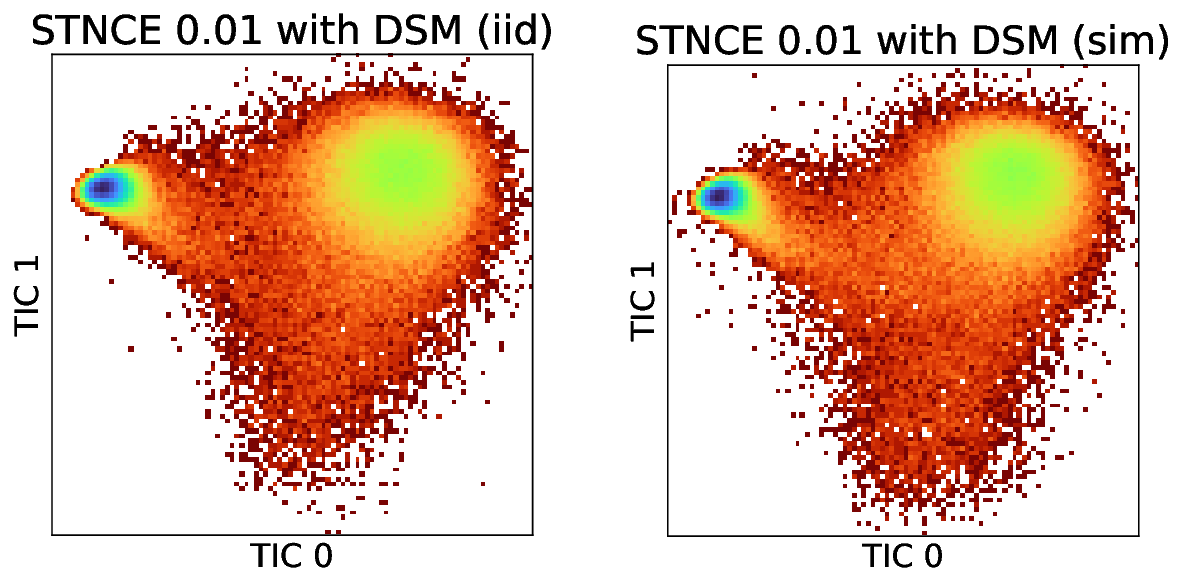
13 Broader impacts↩︎
Our work is relatively theoretical and studies how to train EBMs. Nevertheless, due to the widespread usage of EBMs, it could be used by practioners in malicious manners. We attempt to mitigate such negative impacts by advocating for responsible usage of such trained models.