Branched Signature Kernel Solvers for ODEs with rough Single-Trajectory signals
May 25, 2026
Abstract
We develop a branched signature kernel solver for linear and nonlinear ordinary differential equations driven by a single observed trajectory of a possibly rough forcing signal — a setting common within earthquake engineering, finance, biology, and structural health monitoring, where only one forcing realization is available, and the solver must respect the underlying physical law without an ensemble of realizations. We first introduce a count-sampling construction method to turn the single observation into a hierarchical family of \(N+1\) nested training paths on which the branched signature kernel can be evaluated; this allows the signature kernel machinery, originally designed for multi-realization regression problems, to operate on a single-trajectory observation. Then we build a kernel-collocation framework, which places the ansatz either on the highest-order derivative of the solution or on the solution itself. We prove a universal approximation theorem for the branched signature kernel, leveraging the Hairer–Kelly morphism to express branched signature evaluations through geometric signatures of time-extended paths. The offline solver is extended to a streaming Test/Train/Retrain protocol with optional closed-form online updates in both linear and nonlinear cases. Numerical experiments on six benchmarks show accurate, stable predictions across all regimes.
Keywords: Branched Signature; Branched Signature Kernel; Universal approximation theorem; fractional Brownian motion; Hopf algebra; ODE solver; count sampling; streaming kernel methods.
2000 AMS Mathematics subject classification: 60L10, 60L20, 46E22, 60G17, 65C20, 65C30, 60H10, 91B70.
1 Introduction↩︎
The numerical solution of ordinary differential equations driven by a single observed forcing trajectory arises in many engineering and scientific settings. A structure responding to a recorded ground acceleration during an earthquake, a financial state variable evolving under a single realized market signal, a biological process excited by a particular environmental input, and a coupled oscillator network perturbed by one realization of noise are all instances of the same problem: solve \(\mathcal{N}\mathbf{u}(t)=f(t)\) on \([0,T]\) given a single discrete sample of \(f\). Two features distinguish this regime from the classical setting. First, no ensemble of independent realizations of \(f\) is available, so ensemble-averaged calibration is impossible. Second, the forcing is typically rough: high-frequency seismic accelerations, fractional Brownian motion type volatility, and noisy biological signals all exhibit Hölder regularity well below the bounded-variation assumption of classical numerical analysis. A solver that respects the physical law governing the ODE while learning a representation of the solution from a single rough trajectory is therefore needed.
In the literature, signatures have been successful in encoding path information. Both signatures of geometric rough paths [1], [2] and branched signatures for branched rough paths [3] are fundamental in rough path theory. Uniqueness results of increasing generality were established in [4]–[6], and universal approximation theorems for continuous functions on path space were proved in [6]–[12]. Pairing two signatures via an inner product yields the signature kernel, introduced by [13] by lifting static kernels to path space via the signature transform. [14] characterized the signature kernel as the solution of a Goursat PDE, enabling efficient computation, and [15] developed random Fourier signature features for scalable kernel evaluation. The branched signature model of [16] provides the rough-path foundation for our branched signature kernel; the key difference is that [16] works at the feature-vector level, whereas we work at the reproducing-kernel level, which permits both the universal approximation theorem and the single-trajectory collocation solver developed here.
It is often useful to augment paths before taking signatures, to capture additional structure in data streams. Time, basepoint, and lead–lag augmentations are discussed in [8], [9], [13], [17]; time augmentation guarantees
signature uniqueness and universal approximation [8], [13], while lead–lag augmentation [9], [17], [18] captures quadratic variation and is widely used in finance. [19] introduced learned augmentations via neural networks, leading to the Signatory library. In this paper we view
path augmentation as a transformation that lifts a branched rough path into a geometric rough path; taking the signature kernel of the augmented path then yields the branched signature kernel of the original path. Efficient raw signature implementations
are available in iisignature [20], Signatory [21], PySigLib [22], and KerasSig [23], with Chen’s identity [9] enabling reuse of
sub-path signatures via “stream” features. For signature kernels, KSig [24] provides GPU-accelerated dynamic-programming, low-rank, random-Fourier,
and PDE-based implementations, and PySigLib offers PyTorch-compatible kernel computations with backpropagation. Our count-sampling construction is particularly compatible with these libraries: nested training paths share prefix signatures, so the family
\(\{\boldsymbol{f}_0,\ldots,\boldsymbol{f}_N\}\) can be processed at essentially the cost of the longest path.
Signature-based models have been applied across finance, medicine, and signal processing [7], [9], [25]–[28]. In finance, signatures’ affinity for rough volatility makes them a natural tool for option pricing, nowcasting, and optimal stopping [18], [29]–[33]. For differential equations, the closest precedent to our solver is the signature-kernel path-dependent PDE solver of [34], which fits an RKHS minimum-norm interpolant of the PPDE solution at collocation points but requires multiple realizations of the driving path and does not employ branched signatures. Our framework removes both restrictions: a single trajectory suffices via count-sampling, and the branched signature kernel resolves the higher-order brackets that distinguish branched from geometric roughness. Neural-network signature solvers for path-dependent PDEs have been proposed in [35]–[38] and extended to kernel frameworks in [39]; both again rely on multiple path realizations. The kernel-collocation methodology underlying our solver traces back to the Kansa method [40], [41] for RBF-based PDE solving, with subsequent RBF and RKHS methods for differential equations [42], [43] and Gaussian-process priors for nonlinear PDE solvers [44], which inform our regularization and warm-starting choices in the nonlinear case. Finally, the optional rolling prediction protocol developed here is a kernel-method analogue of online updating: we exploit the block structure of the augmented kernel matrix to update only the newest block in closed form, with periodic full-batch retraining to control drift, paralleling recursive least squares and online kernel ridge regression but, to our knowledge, not previously instantiated for signature-kernel ODE solvers.
Based on the above ideas, we develop a branched signature-kernel collocation solver that operates on a single observed forcing trajectory, the central novelty of this paper. A count-sampling scheme turns one discrete observation into a hierarchical family of nested training paths \(\boldsymbol{f}_0\subset\boldsymbol{f}_1\subset\cdots\subset\boldsymbol{f}_N\), on which the branched signature kernel is natively evaluated and across which Chen’s identity yields prefix-sharing speedups; to our knowledge this single-trajectory training set is new. Building on it, we develop two complementary collocation formulations—a differential ansatz on the highest-order derivative \(\mathbf{u}^{(m)}\) and an integral ansatz on \(\mathbf{u}\) itself, both applicable to multidimensional linear and nonlinear systems. We prove a universal approximation theorem for the branched signature kernel, establishing it as a universal hypothesis class for continuous functionals of the forcing path. Numerically, the branched signature kernel is computed via the Hairer–Kelly morphism [45], whose neural network approximation was first proposed in [16]. The offline solver is extended to a streaming Test/Train/Retrain protocol with either standard Train/Retrain operations or rolling retraining with closed-form \(O(nd^{2}+d^{3})\) online updates in the linear case and scalar Newton steps in the nonlinear case.
The paper is organized as follows. Section 2 introduces signatures and signature kernels. Section 3 presents the branched signature-kernel model and proves a universal approximation theorem. Section 4 develops branched signature-kernel solvers for linear ODE systems, including the linear integral method and its \(m\)-fold-integrated variant, and for nonlinear ODE systems via the nonlinear integral method. Section 5 introduces a standard prediction method along with a streaming protocol with closed-form online updates in the linear case and scalar Newton updates in the nonlinear case, and presents a periodic retraining algorithm. Section 6 presents numerical experiments on an earthquake displacement model, the Solow capital-stock model, an fBM-driven linear ODE, a forced Duffing oscillator, an Arias-intensity-degraded single-degree-of-freedom system with path-dependent coefficients, and a rough Kuramoto phase-oscillator system, with side-by-side comparisons of branched and non-branched constructions.
2 Preliminaries↩︎
In this section, we first provide a self-contained introduction to signatures and signature kernels. We then define the branched signature [16] and the corresponding branched signature kernels.
2.1 Paths and Signatures↩︎
To begin with, we will set some terminology that will help us to talk about signatures and signature kernels.
1. A path \(\mathbf{X}\) from some time interval \([0,T]\) to \(\mathcal{H}\) is a continuous mapping written as \[\mathbf{X}: [0,T] \to \mathcal{H}.\] Also, we define \(\mathbf{X}_{s,t} = \mathbf{X}_t - \mathbf{X}_s\) as an increment of the path.
Unless otherwise stated, we will be working with the paths that take values in the finite dimensional Hilbert space \(\mathcal{H}\) with \(\dim(\mathcal{H}) = d\). Let \(\mathcal{A}\) be the alphabet set corresponding to \(\mathcal{H}\) given as \(\mathcal{A}= \{1,2,\dots,d\}\). We define a word \(\mathbf{w}\) of length \(|\mathbf{w}|=k\) to be sequence \(\mathbf{w}= w_1\cdots w_k\), where \(w_i \in \mathcal{A}\) for \(i=1,2,\dots,k\). Let \(\mathbf{W}\) be the set of all words made from the alphabet \(\mathcal{A}\). Define \[\mathbf{W}_n := \begin{cases} \left\{\mathbf{w}= w_{i_1}\cdots w_{i_k}: |\mathbf{w}| = n\right\}, & n \ne 0,\\ \emptyset, & n=0. \end{cases}\]
2. For two words \(\mathbf{v}= v_1\cdots v_j\) and \(\mathbf{w}= w_1\cdots w_k\) , we define the concatenation \(\mathbf{v}\mathbf{w}\) as \[\mathbf{v}\mathbf{w}= v_1\cdots v_j w_1\cdots w_k.\]
The signature of a path defined on \(\mathcal{H}\) lives in the space called extended tensor algebra over \(\mathcal{H}\) defined as \[T((\mathcal{H})) = \prod_{n=0}^{\infty} (\mathcal{H})^{\otimes n} = \{\mathbf{v}= (v_0, v_1, \dots , v_n, \dots ) \; | \; v_n \in (\mathcal{H})^{\otimes n}, n = 0, 1,\dots \},\] where \((\mathcal{H})^{\otimes 0} := \mathbb{R}\). We also define the tensor algebra over \(\mathcal{H}\) to be the space \(T(\mathcal{H})\) defined by \[T(\mathcal{H}) = \bigoplus_{n=0}^{\infty} (\mathcal{H})^{\otimes n} = \{ \mathbf{v}\in T((\mathcal{H})) \; | \; \forall \; \mathbf{v}\; \exists \; K \in \mathbb{N}\text{ such that } v_n = 0 \; \forall \; n \ge K\},\] where most of the components of the infinite dimensional object \(\mathbf{v}\in T((\mathcal{H}))\) are zero. If we want to restrict the non-zero components then we have the truncated tensor algebra over \(\mathcal{H}\) which is defined as \[T^N(\mathcal{H}) := \left\{ \mathbf{v} \in T(\mathcal{H}) \; | \; v_n = 0 \; \forall \; n > N\right\}.\] Next, define paths of bounded \(p\)-variation for \(p=1\) also called paths of bounded variation.
3. Let \(\mathcal{H}\) be a Hilbert space. We denote the set of \(\mathcal{H}\)-valued paths of bounded variation on \([0,1]\) starting at the origin by \[C^1([0,1], \mathcal{H}):=\left\{\mathbf{X}\in C([0,1], \mathcal{H}): \mathbf{X}(0)=0, \quad\|\mathbf{X}\|_1<\infty\right\}\] where \(\|\mathbf{X}\|_1=\sup _\pi \sum_{i=1}^{l-1}\left\|\mathbf{X}\left(t_{i+1}\right)-\mathbf{X}\left(t_i\right)\right\|_{\mathcal{H}}\) and the supremum is taken over all finite partitions \(\pi=\left\{\left(t_i\right)_{i=1, \ldots, l}: 0=t_1<\cdots<t_l=1\right\}\) of \([0,1]\).
Though we will be working with paths of bounded \(p\)-variation for any \(p \ge 1\), the signature of bounded \(p\)-variation for \(p = 1\) is canonically defined using Riemann–Stieltjes integration.
4. The signature of an \(\mathcal{H}\)-valued path of bounded variation \(\left(\mathbf{X}_t\right)_{t \in [0,T]}\) is an infinite dimensional object \(\mathbf{Sig}(\mathbf{X})_{st}\) that belongs to the space \(T((\mathcal{H}))\) and is defined as \[\mathbf{Sig}(\mathbf{X})_{st} = \left(1, \int_s^t d\mathbf{X}^{w_i}_r, \int_s^t \int_s^{r_2} d\mathbf{X}^{w_i}_{r_1} d\mathbf{X}^{w_j}_{r_2}, \int_s^t \int_s^{r_3}\int_s^{r_2} d\mathbf{X}^{w_i}_{r_1} d\mathbf{X}^{w_j}_{r_2} d\mathbf{X}^{w_k}_{r_3}, \cdots \right)\] Where \({w_i,w_j,w_k, \dots \in \mathcal{A}}\). Equivalently, the signature of a continuous \(\mathcal{H}\)-valued path of bounded variation \((\mathbf{X}_t)_{t \in [0,T]}\) is a \(T((\mathcal{H}))\)-valued process \((s,t) \in \Delta_T^2 \mapsto \mathbf{Sig}(\mathbf{X})_{st} \in T((\mathcal{H}))\) also defined recursively as \[\left\langle \mathbf{Sig}(\mathbf{X})_{st}, \emptyset \right\rangle := 1, \qquad \left\langle \mathbf{Sig}(\mathbf{X})_{st}, \mathbf{w} \right\rangle := \int_{s}^{t} \left\langle \mathbf{Sig}(\mathbf{X})_{sr}, w_1\cdots w_{n-1} \right\rangle d\mathbf{X}^{w_n}_{r},\] for each word \(\mathbf{w}= w_1 \dots w_n \in \mathbf{W}\) and \(\Delta_T^2 := \{ (s,t) \in [0,T]^2 : 0 \leq s \leq t \leq T \}\).
The signature of a path of bounded variation enjoys several structural properties, one being the shuffle product. To describe the shuffle property for signature components, we first define the shuffle product on words \(\mathbf{w}\) in \(\mathbf{W}\).
5. Let \(\emptyset\) denote the empty word. For words \(\mathbf{u},\mathbf{v}\) and letters \(a,b\), the shuffle product is defined recursively by \[\mathbf{u}\shuffle \emptyset = \emptyset \shuffle \mathbf{u}= \mathbf{u}, \qquad (\mathbf{u}a) \shuffle (\mathbf{v}b) = \bigl(\mathbf{u}\shuffle \mathbf{v}b\bigr)a + \bigl(\mathbf{u}a \shuffle \mathbf{v}\bigr)b .\]
Fix a basis \(\{e_1,\dots,e_d\}\) of \(\mathcal{H}\), and for a word \(\mathbf{w}=w_1\cdots w_n\) define \(e_{\mathbf{w}}:=e_{w_1}\otimes\cdots\otimes e_{w_n}\) and \(e_{\emptyset}:=1\). The shuffle product then extends from words to elements of \(T(\mathcal{H})\) by \[\mathbf{x} \shuffle \mathbf{y} = \sum_{\mathbf{u},\mathbf{v}}x_{\mathbf{u}}y_{\mathbf{v}} \left(e_{\mathbf{u}}\shuffle e_{\mathbf{v}}\right),\] where \(\mathbf{x}=\sum_{\mathbf{u}}x_{\mathbf{u}}e_{\mathbf{u}}, \mathbf{y}=\sum_{\mathbf{u}}y_{\mathbf{u}}e_{\mathbf{u}} \in T(\mathcal{H})\). Following this definition, if we endow the space \(T(\mathcal{H})\) with the shuffle product \(\shuffle\) then the quadruple \(\left(T(\mathcal{H}), +, \cdot, \shuffle \right)\) is a commutative associative algebra.
6. Let \((\mathbf{X}_t)_{t \in [0,T]}\) be a continuous \(\mathcal{H}\)-valued path of bounded variation and let \(\mathbf{u}= u_1 \dots u_n\) and \(\mathbf{v}= v_1 \dots v_m\) be two words. The shuffle property states that \[\left\langle \mathbf{Sig}(\mathbf{X})_{st}, \mathbf{u} \right\rangle\, \left\langle \mathbf{Sig}(\mathbf{X})_{st}, \mathbf{v} \right\rangle = \left\langle \mathbf{Sig}(\mathbf{X})_{st}, \mathbf{u}\shuffle \mathbf{v} \right\rangle.\]
7. When \(|\mathbf{u}| = |\mathbf{v}| = 1\), the shuffle property reduces to the classical integration-by-parts identity. See for example, [1].
Another nice property is Chen’s Identity (See [2]). This allows for the concatenation of paths, which we will rely on later in our count method speedup.
8. Let \((\mathbf{X}_t)_{t \in [0,T]}\) be a continuous \(\mathcal{H}\)-valued path of bounded variation. Then the concatenated signature over intervals \([s,u]\) and \([u,t]\) satisfies \[\mathbf{Sig}(\mathbf{X})_{st} = \mathbf{Sig}(\mathbf{X})_{su} \otimes \mathbf{Sig}(\mathbf{X})_{ut}, \qquad 0 \leq s \leq u \leq t \leq T.\] Equivalently, for every word \(\mathbf{w}\in \mathbf{W}\), denote \(\mathbf{u}\mathbf{v}\) as concatenation. We have \[\left\langle \mathbf{Sig}(\mathbf{X})_{st}, \mathbf{w} \right\rangle = \sum_{\mathbf{u}\mathbf{v}= \mathbf{w}} \left\langle \mathbf{Sig}(\mathbf{X})_{su}, \mathbf{u} \right\rangle\, \left\langle \mathbf{Sig}(\mathbf{X})_{ut}, \mathbf{v} \right\rangle.\]
In general, if the signatures of two paths of bounded variation coincide, then the paths agree up to tree-like equivalence [4]. Uniqueness of signatures for time-extended semimartingales was proved in [6]. We will use the following uniqueness theorem for geometric rough paths of time-extended paths (proved in [16]), which is key to using the signature as a feature map that can universally approximate functionals of the underlying path under suitable assumptions.
9. Let \(\mathbf{X},\mathbf{Y}:[0,T]\to\mathbb{R}^d\) be continuous \(\alpha\)-Hölder paths with \(\mathbf{X}_0=\mathbf{Y}_0=0\) for some \(\alpha > \frac{1}{4}\). Form the time-augmented paths \(\widehat{\mathbf{X}}(t):=(t,\mathbf{X}_t)\) and \(\widehat{\mathbf{Y}}(t):=(t,\mathbf{Y}_t)\) in \(\mathbb{R}^{1+d}\). Assume their (geometric) terminal signatures coincide at all levels i.e., \[\mathbf{Sig}(\widehat{\mathbf{X}})_{0,T}=\mathbf{Sig}(\widehat{\mathbf{Y}})_{0,T}.\] Then \(\mathbf{X}_t=\mathbf{Y}_t\) for all \(t\in[0,T]\).
2.2 Kernels and Signature Kernels↩︎
Before defining a signature kernel, we recall standard static kernels and their key properties, since the signature kernel will simply be a kernel on path space.
10. Let \(\mathcal{X}\) be a nonempty set. A function \(\mathbf{K}:\mathcal{X}\times\mathcal{X}\to\mathbb{R}\) is a kernel if there exists a Hilbert space \(\mathcal{H}\) and a map \(\phi:\mathcal{X}\to\mathcal{H}\) such that \[\mathbf{K}(x,x') := \bigl\langle \phi(x),\phi(x') \bigr\rangle_{\mathcal{H}}, \qquad \forall\, x,x'\in\mathcal{X}.\] A kernel \(\mathbf{K}\) is positive definite if it is symmetric and, for every \(n\in\mathbb{N}\), every \(x_1,\ldots,x_n\in\mathcal{X}\), and every \(c_1,\ldots,c_n\in\mathbb{R}\), \[\sum_{i=1}^n\sum_{j=1}^n c_i c_j\,\mathbf{K}(x_i,x_j) > 0.\]
This definition ensures that \(\mathbf{K}\) can be realized as an inner product in some feature space \(\mathcal{H}\), which is exactly the structure we will exploit on path space. Two common example kernels are as follows:
Example 1. The linear kernel between a set of data points \(x,y \in \mathbb{R}^d\) is simply the inner product of the two inputs \[\mathbf{K}(x,y) = \bigl <x,y\bigr>_{\mathbb{R}^d}.\]
Example 2. For \(x,y \in \mathbb{R}^d\), we define the RBF kernel using the squared Euclidean distance \(\|x-y\|_2^2\) and a positive parameter \(\sigma>0\) as follows: \[\mathbf{K}(x,y) = \exp\left(-\frac{\|x-y\|_2^2}{2\sigma^2}\right).\]
The Moore–Aronszajn theorem explains how any positive definite kernel induces a canonical function space, the RKHS, in which kernel methods act as linear models in feature space.
11. For every symmetric positive definite kernel \(\mathbf{K}:\mathcal{X}\times\mathcal{X}\to\mathbb{R}\), there exists a unique Hilbert space \(\mathcal{H}_{\mathbf{K}}\) of functions \(f:\mathcal{X}\to\mathbb{R}\), the reproducing kernel Hilbert space (RKHS)* of \(\mathbf{K}\), satisfying the reproducing property \[\langle f,\,\mathbf{K}(x,\cdot)\rangle_{\mathcal{H}_{\mathbf{K}}} = f(x), \qquad \forall\,f\in\mathcal{H}_{\mathbf{K}},\; x\in\mathcal{X}.\]*
Within an RKHS, the minimum‑norm interpolant formalizes the basic kernel‑collocation idea we will later use with signature kernels.
12. Given distinct points \(x_1,\ldots,x_N\in\Omega\) with values \(y_1,\ldots,y_N\in\mathbb{R}\) and an RKHS \(\mathcal{H}\) over \(\Omega\), the minimum-norm interpolant is \[f^*_{X,Y} = \mathop{\mathrm{argmin}}_{f\in\mathcal{H}}\|f\|_{\mathcal{H}} \quad\text{subject to}\quad f(x_i)=y_i,\quad i=1,\ldots,N.\]
In our setting, we will construct such interpolants on a space of paths, using a kernel built from path signatures.
13. Let \((\mathbf{X}_t)_{t \in [0,T]}\) and \((\mathbf{Y}_t)_{t \in [0,T]}\) take values in \(\mathcal{X}\), and let \(\mathbf{K}:\mathcal{X}\times\mathcal{X}\to\mathbb{R}\) be a positive definite kernel with associated RKHS \(\mathcal{H}\). We lift each path \(\mathbf{X},\mathbf{Y}:[0,T]\to\mathcal{X}\) to the \(\mathcal{H}\)-valued paths \[\mathbf{K}_X(t):=\mathbf{K}(X_t,\cdot)\in\mathcal{H}, \qquad \mathbf{K}_Y(t):=\mathbf{K}(Y_t,\cdot)\in\mathcal{H}.\] Writing \(\mathbf{Sig}(\mathbf{K}_X)\) and \(\mathbf{Sig}(\mathbf{K}_Y)\) for the signatures of the lifted paths, the signature kernel is \[\mathbf{K}_{\mathbf{Sig}}(\mathbf{X},\mathbf{Y}) := \bigl\langle \mathbf{Sig}(\mathbf{K}_X),\mathbf{Sig}(\mathbf{K}_Y)\bigr\rangle_{T((\mathcal{H}))},\] where the inner product is taken over the extended tensor algebra \(T((\mathcal{H}))\) [13].
14. If the paths \(\mathbf{X}_t\) and \(\mathbf{Y}_t\) take values in \(\mathbb{R}^d\), we may take \(\mathcal{X}=\mathbb{R}^d\) and \(\mathbf{K}(x,x')=\langle x,x'\rangle_{\mathbb{R}^d}\), so that \[\mathbf{K}_{\mathbf{Sig}}(\mathbf{X},\mathbf{Y}) = \bigl\langle \mathbf{Sig}(\mathbf{X}),\mathbf{Sig}(\mathbf{Y})\bigr\rangle_{T((\mathbb{R}^d))}.\] Unless otherwise stated, all paths in our consideration will take values in \(\mathbb{R}^d\) for some \(d \ge 1\). For our numerical experiments we use the truncated signature kernel, with the scalar product of the signatures truncated at level \(N\): \[\mathbf{K}^N_{\mathbf{Sig}}(\mathbf{X},\mathbf{Y}) := \bigl\langle \mathbf{Sig}^N(\mathbf{X}),\mathbf{Sig}^N(\mathbf{Y})\bigr\rangle_{T^N(\mathbb{R}^d)},\]
Besides the linear signature kernel, we will also use a Gaussian (RBF) kernel on signature features.
15 (Truncated RBF Signature Kernel). Let \(\mathbf{X}\) and \(\mathbf{Y}\) be paths in \(\mathbb{R}^d\), and let \(\mathbf{Sig}^m(\mathbf{X})\) and \(\mathbf{Sig}^m(\mathbf{Y})\) denote their signatures truncated up to level \(m\). After flattening the truncated signatures into vectors, we define the truncated RBF signature kernel by \[\mathbf{K}_{\mathrm{RBF\text{-}sig}}^{m}(\mathbf{X},\mathbf{Y}) = \exp\left( -\frac{ \left\| \mathbf{Sig}^m(\mathbf{X}) - \mathbf{Sig}^m(\mathbf{Y}) \right\|_2^2 }{2\sigma^2} \right), \qquad \sigma>0.\] Equivalently, using the Euclidean inner product, we can write \[\mathbf{K}_{\mathrm{RBF\text{-}sig}}^{m}(\mathbf{X},\mathbf{Y}) = \exp\left( -\frac{ \left\| \mathbf{Sig}^m(\mathbf{X}) \right\|_2^2 + \left\| \mathbf{Sig}^m(\mathbf{Y}) \right\|_2^2 -2 \left\langle \mathbf{Sig}^m(\mathbf{X}), \mathbf{Sig}^m(\mathbf{Y}) \right\rangle}{2\sigma^2} \right).\]
2.3 Kernel Matrices and Signature Normalizations↩︎
We next describe simple normalizations of signature features and the associated kernel Gram matrices used in our experiments. Throughout this subsection, let \(\mathbf{X}_1,\ldots,\mathbf{X}_n\) be paths in \(\mathbb{R}^d\), let \(S_i := \mathbf{Sig}^m(\mathbf{X}_i) \in \mathbb{R}^M\) denote their flattened truncated signatures, where \(M = \sum_{k=0}^{m} d^k\), and let \(S \in \mathbb{R}^{n\times M}\) be the matrix with \(S_i\) as its \(i\)-th row.
16 (Robust signature matrix). The robust signature matrix \(S_{\mathrm{robust}} \in \mathbb{R}^{n\times M}\) is defined coordinate-wise by \[(S_{\mathrm{robust}})_{ij} = \frac{S_{ij} - \mu_j}{\operatorname{IQR}_j}, \qquad i=1,\ldots,n,\quad j=1,\ldots,M,\] where \(\mu_j\) and \(\operatorname{IQR}_j = Q_{0.75}-Q_{0.25}\) are the column-wise median and inter-quartile range of \(S\).
This transformation rescales each signature coordinate using robust statistics, improving conditioning when constructing the following gram matrices.
17. The linear signature kernel Gram matrix \(\mathbb{K}= SS^\top \in \mathbb{R}^{n\times n}\) has entries \[\mathbb{K}_{ij} = \left\langle \mathbf{Sig}^m(\mathbf{X}_i), \mathbf{Sig}^m(\mathbf{X}_j) \right\rangle, \qquad i,j=1,\ldots,n.\]
Thus \(\mathbb{K}\) is simply the Gram matrix of the truncated signature feature vectors under the Euclidean inner product. We may instead apply the Gaussian kernel, providing a nonlinear similarity measure between paths.
18. The RBF signature kernel Gram matrix \(\mathbb{K}\in \mathbb{R}^{n\times n}\) has entries \[\mathbb{K}_{ij} = \exp\!\left( -\frac{\|S_i - S_j\|_2^2}{2\sigma^2} \right), \qquad i,j=1,\ldots,n,\quad \sigma>0.\]
2.4 Sampling methods and Count Method Speedup↩︎
We now describe a novel way to turn a single discretized path into a nested family of training paths and explain how this structure accelerates signature and signature-kernel computations.
19 (Count-sampling method). Let \(\mathbf{X}= (X^1, \ldots, X^d) : [0, T] \to \mathbb{R}^d\) be a path discretized at \(N\) points \(0 = t_0 < t_1 < \cdots < t_{N-1} = T\), and write \(\mathbf{X}_{0,\, t_j}\) for the restriction of \(X\) to the prefix interval \([0, t_j]\). The count-sampling construction produces the family of \(N\) nested training paths \[\mathbf{X}_0 := \mathbf{X}_{t_0,\, t_0},\qquad \mathbf{X}_1 := \mathbf{X}_{0,\, t_1},\qquad \ldots,\qquad \mathbf{X}_{N} := \mathbf{X}_{0,\, T}.\] The first sample \(\mathbf{X}_0\) is the degenerate two-point path \((\mathbf{X}(0), \mathbf{X}(0))\), so that \(\mathbf{X}_0\) has at least two values and the signature kernel is well-defined on it. This convention lets the initial point be treated uniformly with the longer prefixes and is used by the algorithms below.
20. All count-sampled paths \(\mathbf{X}_0, \ldots, \mathbf{X}_{N-1}\) share the starting point \(\mathbf{X}(0)\) but differ in length: \(\mathbf{X}_j\) is supported on \([0, t_j]\) and contains strictly more path information than its predecessors. From a single observed time series we therefore obtain a hierarchical training set of \(N\) nested paths, ideally suited as inputs to the signature kernel \(\mathbf{K}_{\mathbf{Sig}}\). Throughout the rest of the section, “training paths \(\mathbf{X}_0, \ldots, \mathbf{X}_{N-1}\)” refers to this construction.
When using the count-sampling method, one can exploit Chen’s identity to greatly reduce computational cost. Two popular signature libraries, keras-sig and signatory, expose this speedup through a stream argument
and support GPU acceleration; we rely on these implementations in our numerical experiments.
Suppose we use the count-sampling method to generate \(N\) nested training paths \(\mathbf{X}_0, \mathbf{X}_1, \dots, \mathbf{X}_{N-1}\), each of dimension \(d\). The \(j\)-th path has length \[L_j = \begin{cases} 2, & j=0,\\ j+1, & j \ge 1, \end{cases}\] with \(L_0 = 2\) ensuring that even the shortest path admits a well-defined truncated signature; this convention is immaterial for the asymptotics. (Here \(N\) is the number of count-sampled paths in this section; this corresponds to \(N{+}1\) in the collocation setup, where paths were indexed \(\mathbf{X}_0,\ldots,\mathbf{X}_N\).)
In most numerical libraries, path tensors have shape \((B,L,D)\), where \(B\) is the batch size, \(L\) the path length, and \(D\) the path dimension. The naive approach therefore produces \(N\) separate tensors of size \((1, L_j, d)\) and calls the signature routine on each independently. By the analysis of [21], computing the truncated signature of a single length-\(L\) path to depth \(M\) costs \((L-1)\cdot O(d^M)\), so summing over all prefixes yields a total cost of order \[O\!\left(\sum_{j=0}^{N-1} (L_j - 1)\,d^M\right) = O\!\left(\left(1 + \tfrac{N(N-1)}{2}\right)d^M\right) = O(N^2 d^M).\]
With the count-method speedup, we instead pass only the final prefix tensor of size \((1,N,d)\) to the signature function. It processes the entire stream from left to right, and Chen’s identity \[\mathbf{Sig}^M(\mathbf{X}_{[t_0,t_{j+1}]}) = \mathbf{Sig}^M(\mathbf{X}_{[t_0,t_j]}) \otimes \mathbf{Sig}^M(\mathbf{X}_{[t_j,t_{j+1}]})\] allows us to reuse all previously computed leading increments. The total time complexity becomes \[(N-1)\cdot O(d^M) = O(N d^M),\] an order-\(N\) improvement over the naive \(O(N^2 d^M)\) scaling. These methods are displayed in Table 1.
| Method | Time |
|---|---|
| Naive (independent calls) | \(O(N^2 d^M)\) |
| Count method | \(O(N d^M)\) |
Now consider computing the truncated signature-kernel Gram matrix of the prefix paths up to depth \(M\). Previous methods either rely on dynamic-programming techniques [13] or on PDE approximations exploiting the fact that the signature kernel satisfies a Goursat PDE [14]; both are implemented efficiently in the Python package PySigLib. The Goursat approach has cost \(O(N^2 L^2 d)\), and since the maximum path
length satisfies \(L = N\) in our count-sampled setting, this becomes \(O(N^4 d)\). A dynamic-programming approach yields \(O(N^2 L^2 M d) = O(N^4 M d)\) for
the same \(N \times N\) kernel matrix.
With the count speedup, we first compute the truncated signatures in \(O(N d^M)\) time, producing an \(N \times C\) matrix of signature vectors \(S\), where row \(j\) holds \(\mathbf{Sig}^M(\mathbf{X}_j)\) flattened into a vector of length \(C = \sum_{k=0}^{M} d^k = O(d^M)\). To form the kernel Gram matrix we then compute \(K = S S^{\top}\), a matrix multiplication costing \(O(N^2 d^M)\). The overall runtime is therefore \(O(N^2 d^M)\), in which the matrix multiplication dominates the signature-computation step. Runtimes for all methods are summarized in Table 2.
| Method | Time |
|---|---|
| Goursat PDE | \(O(N^4 d)\) |
| Dynamic programming | \(O(N^4 M d)\) |
| Count method | \(O(N^2 d^M)\) |
The Goursat and dynamic-programming methods inherit only a linear \(d\)-dependence from the static-kernel evaluations they invoke. The count method, by contrast, materializes the full truncated signature vector of length \(O(d^M)\) and pays for it explicitly in the Gram matrix multiplication. The two regimes therefore exchange a quartic \(N^4\) scaling for an exponential \(d^M\) scaling — a favorable trade-off whenever \[N \;\gtrsim\; d^{(M-1)/2},\] obtained by equating \(N^4 d\) with \(N^2 d^M\). Our experiments operate in the regime where \(N\) is large and \(M\) is small — the branched signature framework lets us extract sufficient path-wise information at low truncation depth — so the \(N^4 \to N^2\) improvement dominates the unfavorable \(d \to d^M\) trade-off. This regime is exactly the one encountered in time-series data-driven modeling, where long observation records produce many nested prefix paths but only modest signature depth is needed, and the count-method speedup is therefore decisive.
2.5 Signature kernel for geometric rough path↩︎
In this subsection, we extend the signature kernel from paths of bounded variation to geometric rough paths. In general, \(\alpha\)-Hölder paths with \(\alpha > \frac{1}{4}\) admit geometric rough path lifts, and by Lyons’ extension theorem [2], the signatures of these lifts are well-defined at all higher levels. This allows us to define the signature kernel for such geometric rough paths as follows, see [13].
21. Let \((\mathbf{X}_t)_{t \in [0,T]}\) and \((\mathbf{Y}_t)_{t \in [0,T]}\) be \(\alpha\)-Hölder paths with \(\alpha > \tfrac{1}{4}\) taking values in \(\mathbb{R}^d\), and let \(\mathbf{Sig}(\mathbf{X})\) and \(\mathbf{Sig}(\mathbf{Y})\) be their signatures defined by Lyons’ extension theorem. The signature kernel \(\mathbf{K}_{\mathbf{Sig}}(\mathbf{X},\mathbf{Y})\) is defined for these paths as \[\mathbf{K}_{\mathbf{Sig}}(\mathbf{X},\mathbf{Y}) := \bigl\langle \mathbf{Sig}(\mathbf{X}),\mathbf{Sig}(\mathbf{Y}) \bigr\rangle_{T((\mathbb{R}^d))},\] where \[\bigl\langle \mathbf{Sig}(\mathbf{X}),\mathbf{Sig}(\mathbf{Y}) \bigr\rangle_{T((\mathbb{R}^d))} := \sum_{n=0}^{\infty} \bigl\langle \pi_n\bigl(\mathbf{Sig}(\mathbf{X})\bigr),\pi_n\bigl(\mathbf{Sig}(\mathbf{Y})\bigr) \bigr\rangle_{(\mathbb{R}^d)^{\otimes n}},\] whenever the series is well-defined. Here \(\pi_n(\mathbf{Sig}(\mathbf{X}))\in(\mathbb{R}^d)^{\otimes n}\) denotes the level-\(n\) signature component of \(\mathbf{X}\). Equivalently, if \(\mathbf{w}= w_1\dots w_n\) is a word of length \(n\) from the set of words \(\mathbf{W}\), then \[\mathbf{K}_{\mathbf{Sig}}(\mathbf{X},\mathbf{Y}) = \sum_{n=0}^{\infty} \sum_{|\mathbf{w}|=n} \langle \mathbf{Sig}(\mathbf{X}),\mathbf{w}\rangle\, \langle \mathbf{Sig}(\mathbf{Y}),\mathbf{w}\rangle.\]
We now state and prove a universal approximation theorem for the signature kernel on geometric rough paths by combining this definition with the universal approximation theorem for signatures of geometric rough paths.
22 (Universal approximation theorem for signature kernel). Let \(\mathcal{K}\) be the compact set of paths that admit a geometric rough path lift i.e., \[\mathcal{K}\subset \left\{\mathbf{X}: [0,T] \to \mathbb{R}^d \text{ such that } \mathbf{X}\text{ admits a geometric rough path lift}\right\}.\] Define the compact set of time extended paths \(\widehat{\mathcal{K}}\) as \[\widehat{\mathcal{K}} \subset \left\{\widehat{\mathbf{X}}_t:= (t, \mathbf{X}_t) \text{ such that } \mathbf{X}_t \in \mathcal{K}\right\}.\] Then for every continuous function \(f(\widehat{\mathcal{K}}; \mathbb{R})\) and every \(\epsilon > 0\), there exist an integer \(N \ge 0\), paths \(\widehat{\mathbf{Y}}^1, \dots, \widehat{\mathbf{Y}}^M \in \widehat{\mathcal{K}}\), and scalars \(\alpha_1, \dots \alpha_M\) such that \[\sup_{\widehat{\mathbf{X}} \in \widehat{\mathcal{K}}} \left| f\left(\mathbf{Sig}^p(\widehat{\mathbf{X}})\right) - \sum_{i=1}^{M} \alpha_i \mathbf{K}^N_{\mathbf{Sig}}(\widehat{\mathbf{X}},\widehat{\mathbf{Y}}^i) \right| <\varepsilon,\] where \(\mathbf{Sig}^p(\widehat{\mathbf{X}})\) is the geometric rough path lift of \(\widehat{\mathbf{X}}\) for some \(p \in \mathbb{N}\) depending on the Hölder regularity of \(\mathbf{X}\).
Proof. Leveraging the universal approximation theorem for signatures of geometric rough paths [16],
we have that for every \(f\in C(\widehat{\mathcal{K}};\mathbb{R})\) and every \(\varepsilon>0\), there exist \(N\geq 0\) and \(\ell\in T^{(N)}(\mathbb{R}^{d+1})\) such that \[\label{sig32UAT}
\sup_{\widehat{\mathbf{X}}\in\widehat{\mathcal{K}}}
\left|
f\left(\mathbf{Sig}^p(\widehat{\mathbf{X}})\right)
-
\left\langle
\mathbf{Sig}^N(\widehat{\mathbf{X}})
, \ell \right\rangle
\right|
<\varepsilon.\tag{1}\] Now, let \[M_N
:=
\operatorname{span}
\left\{
\mathbf{Sig}^N(\widehat{\mathbf{Y}})
:
\widehat{\mathbf{Y}}\in\widehat{\mathcal{K}}
\right\}
\subset T^{(N)}(\mathbb{R}^{d+1}).\] Let \(\mathcal{P}_{M_N}\) be the orthogonal projection onto \(M_N\), and define \[\ell_N:=\mathcal{P}_{M_N}\ell.\] For every \(\widehat{\mathbf{X}}\in\widehat{\mathcal{K}}\), we have \[\mathbf{Sig}^N(\widehat{\mathbf{X}})\in M_N.\]
Therefore, \[\left\langle \mathbf{Sig}^N(\widehat{\mathbf{X}}),\ell \right\rangle
=
\left\langle \mathbf{Sig}^N(\widehat{\mathbf{X}}), \mathcal{P}_{M_N}\ell \right\rangle
=
\left\langle \mathbf{Sig}^N(\widehat{\mathbf{X}}), \ell_N \right\rangle.\] Since \(\ell_N\in M_N\), by the definition of \(M_N\), there exist \(\widehat{\mathbf{Y}}^{1},\ldots,\widehat{\mathbf{Y}}^{M}\in\widehat{\mathcal{K}}\) and scalars
\(\alpha_1,\ldots,\alpha_M\in\mathbb{R}\) such that \[\ell_N
=
\sum_{i=1}^{M}
\alpha_i
\mathbf{Sig}^N(\widehat{\mathbf{Y}}^{i}).\] Hence, for every \(\widehat{\mathbf{X}}\in\widehat{\mathcal{K}}\), \[\begin{align}
\left\langle
\mathbf{Sig}^N(\widehat{\mathbf{X}}), \ell
\right\rangle
&=
\left\langle
\mathbf{Sig}^N(\widehat{\mathbf{X}}), \ell_N
\right\rangle
=
\left\langle
\mathbf{Sig}^N(\widehat{\mathbf{X}}),
\sum_{i=1}^{M}
\alpha_i
\mathbf{Sig}^N(\widehat{\mathbf{Y}}^{i})
\right\rangle \\
&=
\sum_{i=1}^{M}
\alpha_i
\left\langle
\mathbf{Sig}^N(\widehat{\mathbf{X}}),
\mathbf{Sig}^N(\widehat{\mathbf{Y}}^{i})
\right\rangle
=
\sum_{i=1}^{M}
\alpha_i
\mathbf{K}_{\mathbf{Sig}}^{N}(\widehat{\mathbf{X}},\widehat{\mathbf{Y}}^{i}).
\end{align}\] Combining this identity with 1 gives \[\sup_{\widehat{\mathbf{X}} \in \widehat{\mathcal{K}}}
\left|
f\left(\mathbf{Sig}^p(\widehat{\mathbf{X}})\right)
-
\sum_{i=1}^{M}
\alpha_i
\mathbf{K}^N_{\mathbf{Sig}}(\widehat{\mathbf{X}},\widehat{\mathbf{Y}}^i)
\right|
<\varepsilon.\] This proves the theorem. ◻
3 Branched Signature Kernel↩︎
In this section we first define the branched signature and the branched signature kernel. We then describe some avaliable ways to construct the branches signature components though lifting paths.
3.1 Branched Signature Kernel↩︎
To begin with, let us define a Hopf algebra and Connes–Kreimer Hopf algebra of rooted trees, a special example of Hopf algebra where branched signature lives.
A Hopf algebra \(\mathscr{H}\) is an algebraic structure that contains a product \(\cdot : \mathscr{H}\hat{\otimes} \mathscr{H}\to \mathscr{H}\), which tells how to combine two objects; a coproduct \(\Delta: \mathscr{H}\to \mathscr{H}\hat{\otimes} \mathscr{H}\), which tells how to split an object; and an antipode \(\mathcal{S}: \mathscr{H}\to \mathscr{H}\), which is the way to encode inverses. Let \(\mathscr{H}^*\) be the dual of \(\mathscr{H}\). The product \(\star\) on the dual space \(\mathscr{H}^*\) is defined via coproduct on \(\mathscr{H}\) as \[\left\langle f \star g, h \right\rangle = \left\langle f \; \hat{\otimes}\; g, \Delta h \right\rangle,\] for any \(f,g \in \mathscr{H}^*\) and \(h \in \mathscr{H}\).
The Connes–Kreimer Hopf algebra of rooted trees is a special type of Hopf algebra which is used in the setting of branched rough paths and branched signatures. The iterated integrals for geometric rough paths are encoded by words \(\mathbf{w}\) made from the alphabet \(\mathcal{A}= \{1,2,\dots,d\}\). However, in the case of branched rough paths, the iterated integrals are encoded by decorated rooted trees, with decorations coming from the set \(\mathcal{A}\). For instance, the iterated integral \[\int_s^t \left(\int_s^u d\mathbf{X}^{i}_r\right) \left(\int_s^u d\mathbf{X}^{j}_r\right) d\mathbf{X}^{k}_u\] is encoded by the tree \[\Forest{decorated[k[i][j]]}.\] The Connes–Kreimer Hopf algebra of rooted trees \(\mathscr{H}\) [46] is the polynomial algebra in which rooted trees play the role of variables. The product of trees is given by placing trees side by side to form a forest, while the coproduct is given by all possible ways of cutting a tree into smaller trees. The Connes–Kreimer Hopf algebra of rooted trees \(\mathscr{H}\) is the appropriate algebraic structure in which the branched signature lives. The definition of the branched signature follows from [3].
23. Let \(\mathcal{A}=\{1,\dots,d\}\) be an alphabet set for a given \(d\)-dimensional path \(\mathbf{X}: [0,T] \to \mathbb{R}^d\). Let \(\mathcal{T}\) be the set of rooted trees with vertices decorated by letters in \(\mathcal{A}\). Let \(\mathscr{H}\) be the Connes–Kreimer Hopf algebra of rooted trees generated by trees is \(\mathcal{T}\), with product given by disjoint union of forests and unit \(\mathbf{1}\). We define branched signature of \(\mathbf{X}\) as a functional on \(\mathscr{H}\) given by \[\mathbf{BSig}(\mathbf{X})_{st} = \sum\limits_{\tau \; \in \; \mathcal{T}, \; |\tau| \; \le \; N} \left\langle \mathbf{BSig}(\mathbf{X})_{st},\tau \right\rangle \mathsf e_{\tau},\] where for each \(\tau \in \mathscr{H}\) the component \(\left\langle \mathbf{BSig}(\mathbf{X})_{st},\tau \right\rangle\) of the branched signature is recursively defined as \[\left\langle \mathbf{BSig}(\mathbf{X})_{st},\mathbf{1} \right\rangle = 1, \quad \text{ and } \quad \left\langle \mathbf{BSig}(\mathbf{X})_{st},\tau \right\rangle = \int_s^t \left\langle \mathbf{BSig}(\mathbf{X})_{su},\tau' \right\rangle d\mathbf{x}^{\mathbf{r}}_u,\] where \(\tau\) is the tree that we get by grafting the root vertex \(\mathbf{r}\) to \(\tau'\) i.e., \(\tau = [\tau']_{\mathbf{r}}\).
24 (Branched signature kernel). Let \(\left(\mathbf{X}_t\right)_{t \in [0,T]}\) and \(\left(\mathbf{Y}_t\right)_{t \in [0,T]}\) be \(\alpha\)-Hölder paths for \(\alpha > \frac{1}{4}\) taking values in \(\mathbb{R}^d\). Let \(\mathbf{BSig}(\mathbf{X})\) and \(\mathbf{BSig}(\mathbf{Y})\) denote their branched signatures, whose components are indexed by decorated rooted forests in the Connes–Kreimer Hopf algebra \(\mathscr{H}\). The branched signature kernel \(\mathbf{K}_{\mathbf{BSig}}(\mathbf{X},\mathbf{Y})\) is defined as \[\mathbf{K}_{\mathbf{BSig}}(\mathbf{X},\mathbf{Y}) := \left\langle \mathbf{BSig}(\mathbf{X}),\mathbf{BSig}(\mathbf{Y}) \right\rangle_{\mathscr{H}^*},\] where \[\left\langle \mathbf{BSig}(\mathbf{X}),\mathbf{BSig}(\mathbf{Y}) \right\rangle_{\mathscr{H}^*} := \sum_{n=0}^{\infty} \left\langle \pi_n\left(\mathbf{BSig}(\mathbf{X})\right), \pi_n\left(\mathbf{BSig}(\mathbf{Y})\right) \right\rangle_{\mathscr{H}_{n}^*},\] whenever the series makes sense. Also, \[\pi_n\left(\mathbf{BSig}(\mathbf{X})\right)\in \mathscr{H}_{n}^*\] denotes the degree-\(n\) component of the branched signature and \(\mathscr{H}_{n}^*\) denotes the dual of the space spanned by decorated rooted forests with exactly \(n\) vertices.
Equivalently, if \(\mathcal{F}_n\) denotes the set of decorated rooted forests of degree \(n\), then \[\mathbf{K}_{\mathbf{BSig}}(\mathbf{X},\mathbf{Y}) = \sum_{n=0}^{\infty} \sum_{\tau\in \mathcal{F}_n} \left\langle \mathbf{BSig}(\mathbf{X}),\tau\right\rangle \left\langle \mathbf{BSig}(\mathbf{Y}),\tau\right\rangle.\]
We prove the universal approximation theorem for the branched signature kernel below.
25. Let \(\mathcal{K}\) be the compact subset of paths that admit a branched rough path lift, \[\mathcal{K}\subset \left\{\mathbf{X}: [0,T] \to \mathbb{R}^d \text{ such that } \mathbf{X}\text{ admits a branched rough path lift}\right\}.\] Define the compact set of time extended paths \(\widehat{\mathcal{K}}\) as \[\widehat{\mathcal{K}} \subset \left\{\widehat{\mathbf{X}}_t:= (t, \mathbf{X}_t) \text{ such that } \mathbf{X}_t \in \mathcal{K}\right\}.\] Then for every continuous function \(f(\widehat{\mathcal{K}}; \mathbb{R})\) and every \(\epsilon > 0\), there exist an integer \(N \ge 0\), paths \(\widehat{\mathbf{Y}}^1, \dots, \widehat{\mathbf{Y}}^M \in \widehat{\mathcal{K}}\), and scalars \(\alpha_1, \dots \alpha_M\) such that \[\sup_{\widehat{\mathbf{X}} \in \widehat{\mathcal{K}}} \left| f\left(\mathbf{BSig}^p(\widehat{\mathbf{X}})\right) - \sum_{i=1}^{M} \alpha_i \mathbf{K}^N_{\mathbf{BSig}}(\widehat{\mathbf{X}},\widehat{\mathbf{Y}}^i) \right| <\varepsilon,\] where \(\mathbf{BSig}^p(\widehat{\mathbf{X}})\) is the branched rough path lift of \(\widehat{\mathbf{X}}\) for some \(p \in \mathbb{N}\) depending on the Hölder regularity of \(\mathbf{X}\).
Proof. Using the universal approximation theorem for signatures of branched rough paths [16], we have
that for every \(f\in C(\widehat{\mathcal{K}};\mathbb{R})\) and every \(\varepsilon>0\), there exist \(N\geq 0\) and \(\tau\in
\mathscr{H}\) such that \[\label{bsig32UAT}
\sup_{\widehat{\mathbf{X}}\in\widehat{\mathcal{K}}}
\left|
f\left(\mathbf{BSig}^p(\widehat{\mathbf{X}})\right)
-
\left\langle
\mathbf{BSig}^N(\widehat{\mathbf{X}})
, \tau \right\rangle
\right|
<\varepsilon,\tag{2}\] where \(\mathscr{H}\) is the Hopf algebra of decorated rooted trees with the decoration coming from \(\mathcal{A}\cup \{0\}\) with \(\mathcal{A}:= \{ 1,2,\dots,d\}\) and \(0\) corresponding to the time component. Now, let \[M_N
:=
\operatorname{span}
\left\{
\mathbf{BSig}^N(\widehat{\mathbf{Y}})
:
\widehat{\mathbf{Y}}\in\widehat{\mathcal{K}}
\right\}
\subset \mathscr{H}^*.\] Let \(\mathcal{P}_{M_N}\) be the orthogonal projection onto \(M_N\), and define \[\tau_N:=\mathcal{P}_{M_N}\tau.\] For every
\(\widehat{\mathbf{X}}\in\widehat{\mathcal{K}}\), we have \[\mathbf{BSig}^N(\widehat{\mathbf{X}})\in M_N.\] Therefore, \[\left\langle
\mathbf{BSig}^N(\widehat{\mathbf{X}}),\tau \right\rangle
=
\left\langle \mathbf{BSig}^N(\widehat{\mathbf{X}}), \mathcal{P}_{M_N}\tau \right\rangle
=
\left\langle \mathbf{BSig}^N(\widehat{\mathbf{X}}), \tau_N \right\rangle.\] Since \(\tau_N\in M_N\), by the definition of \(M_N\), there exist \(\widehat{\mathbf{Y}}^{1},\ldots,\widehat{\mathbf{Y}}^{M}\in\widehat{\mathcal{K}}\) and scalars
\(\alpha_1,\ldots,\alpha_M\in\mathbb{R}\) such that \[\tau_N
=
\sum_{i=1}^{M}
\alpha_i
\mathbf{BSig}^N(\widehat{\mathbf{Y}}^{i}).\]
Hence, for every \(\widehat{\mathbf{X}}\in\widehat{\mathcal{K}}\), \[\begin{align} \left\langle \mathbf{BSig}^N(\widehat{\mathbf{X}}), \tau \right\rangle &= \left\langle \mathbf{BSig}^N(\widehat{\mathbf{X}}), \tau_N \right\rangle = \left\langle \mathbf{BSig}^N(\widehat{\mathbf{X}}), \sum_{i=1}^{M} \alpha_i \mathbf{BSig}^N(\widehat{\mathbf{Y}}^{i}) \right\rangle \\ &= \sum_{i=1}^{M} \alpha_i \left\langle \mathbf{BSig}^N(\widehat{\mathbf{X}}), \mathbf{BSig}^N(\widehat{\mathbf{Y}}^{i}) \right\rangle = \sum_{i=1}^{M} \alpha_i \mathbf{K}_{\mathbf{BSig}}^{N}(\widehat{\mathbf{X}},\widehat{\mathbf{Y}}^{i}). \end{align}\] Combining this identity with 2 gives \[\sup_{\widehat{\mathbf{X}} \in \widehat{\mathcal{K}}} \left| f\left(\mathbf{BSig}^p(\widehat{\mathbf{X}})\right) - \sum_{i=1}^{M} \alpha_i \mathbf{K}^N_{\mathbf{BSig}}(\widehat{\mathbf{X}},\widehat{\mathbf{Y}}^i) \right| <\varepsilon.\] This proves the claim. ◻
Instead of computing the branched signature kernel of the paths \(\mathbf{X}\) and \(\mathbf{Y}\), we compute the geometric signature kernel of the extended paths \(\Bar{\mathbf{X}}\) and \(\Bar{\mathbf{Y}}\) and leverage the Hairer–Kelly morphism [45] to show that the geometric signature kernel of extended paths gives the information that a branched signature kernel contains.
The Hairer–Kelly morphism \(\Psi\) is a Hopf algebra morphism from the Connes–Kreimer Hopf algebra of rooted trees \(\mathscr{H}\) to shuffle Hopf algebra over vector space \(\mathcal{V}\) spanned by rooted trees i.e., \[\Psi: (\mathscr{H}, \cdot, \Delta) \to (T(\mathcal{V}), \shuffle, \Bar{\Delta}).\] For a tree \(\tau \in \mathcal{F}_n\), the morphism \(\Psi\) is defined as \[\Psi(\tau) = \tau + \Psi_{n-1}(\tau),\] where \(\Psi_{n-1}(\tau)\) is all the smaller trees coming from cutting the tree \(\tau\) in all possible ways.
The existence of such a morphism \(\Psi\) and the extended path \(\Bar{\mathbf{X}}\) is proved in [45]. The main theorem in the paper states that for a branched rough path \(\mathbf{BSig}^N(\mathbf{X})\), one can construct the extended path \(\Bar{\mathbf{X}}\) and the geometric rough path \(\mathbf{Sig}^N(\mathbf{X})\) such that \[\left\langle \mathbf{BSig}^N(\mathbf{X})_{st}, \tau \right\rangle = \left\langle \mathbf{Sig}^N(\Bar{\mathbf{X}})_{st}, \Psi(\tau) \right\rangle,\] for all \(\tau \in \mathcal{F}_n\).
This result can also be applied to branched and geometric signatures using the extension theorems from rough paths to signatures. We state and prove the universal approximation theorem that claims that any function of the branched rough path can be approximated by the signature kernel of the extended paths. The precise statement and proof of the theorem are given as follows.
26. Let \(\mathcal{K}\) be the compact subset of time-extended paths that admit a branched rough path lift i.e., \[\mathcal{K}\subset \left\{\mathbf{X}: [0,T] \to \mathbb{R}^{d+1} \text{ such that } \mathbf{X}= (t,\mathbf{X}^-) \text{ and } \mathbf{X}^- \text{ admits a branched rough path lift}\right\}\] Then for every continuous function \(f(\mathcal{K}; \mathbb{R})\) and every \(\epsilon > 0\), there exist an integer \(N \ge 0\), paths \(\mathbf{Y}^1, \dots, \mathbf{Y}^M \in \mathcal{K}\), and scalars \(\alpha_1, \dots \alpha_M\) such that \[\sup_{\mathbf{X}\in \mathcal{K}} \left| f\left(\mathbf{BSig}^p(\mathbf{X})\right) - \sum_{i=1}^{M} \alpha_i \mathbf{K}^N_{\Psi, \mathbf{Sig}}(\Bar{\mathbf{X}},\Bar{\mathbf{Y}}^i) \right| <\varepsilon,\] where \(\mathbf{BSig}^p(\mathbf{X})\) is the branched rough path lift of \(\mathbf{X}\) for some \(p \in \mathbb{N}\) depending on the Hölder regularity of \(\mathbf{X}^{-}\), \(\Bar{\mathbf{X}},\Bar{\mathbf{Y}}^i\) are the extended paths constructed via extension map of Hairer-Kelly, and \(\mathbf{K}^N_{\Psi, \mathbf{Sig}}(\Bar{\mathbf{X}},\Bar{\mathbf{Y}}^i)\) is defined as \[\mathbf{K}^N_{\Psi, \mathbf{Sig}}(\Bar{\mathbf{X}},\Bar{\mathbf{Y}}^i) := \sum_{n=0}^{N} \sum_{\tau\in \mathcal{F}_n} \left\langle \mathbf{Sig}(\Bar{\mathbf{X}}),\Psi(\tau)\right\rangle \left\langle \mathbf{Sig}(\Bar{\mathbf{Y}^i}),\Psi(\tau)\right\rangle.\]
Proof. By the extension of Hairer-Kelly, for a path \(\mathbf{X}\) that admits a branched rough path, there exists a map \(\Psi\) and an extended path \(\Bar{\mathbf{X}}\) such that each component of the branched signature corresponding a tree \(\tau \in \mathscr{H}\) can be identified as the component of signature of \(\Bar{\mathbf{X}}\) corresponding to \(\Psi(\tau) \in T(\mathcal{V})\) i.e., \[\left\langle \mathbf{BSig}(\mathbf{X}), \tau \right\rangle = \left\langle \mathbf{Sig}(\Bar{\mathbf{X}}), \Psi(\tau) \right\rangle.\] This should also be true for truncated signatures. Therefore, for paths \(\mathbf{X}\) and \(\mathbf{Y}_i\) \[\begin{align} \mathbf{K}^N_{\mathbf{BSig}}(\mathbf{X},\mathbf{Y}^i) & = \sum_{n=0}^{N} \sum_{\tau\in \mathcal{F}_n} \left\langle \mathbf{BSig}(\mathbf{X}),\tau\right\rangle \left\langle \mathbf{BSig}(\mathbf{Y}^i),\tau\right\rangle\\ & = \sum_{n=0}^{N} \sum_{\tau\in \mathcal{F}_n} \left\langle \mathbf{Sig}(\Bar{\mathbf{X}}),\Psi(\tau)\right\rangle \left\langle \mathbf{Sig}(\Bar{\mathbf{Y}^i}),\Psi(\tau)\right\rangle = \mathbf{K}^N_{\Psi, \mathbf{Sig}}(\Bar{\mathbf{X}},\Bar{\mathbf{Y}}^i). \end{align}\] Hence, the claim follows by Theorem 25. ◻
3.2 Path Lifts↩︎
The universal approximation theorems above guarantee that any continuous functional of a branched rough path can be approximated via the signature kernel of an extended path \(\Bar{\mathbf{X}}\), but they do not prescribe how to construct the extension. We consider two approaches: an explicit \(t\)–value lift, and a learned neural network lift.
27 (\(t\)–value lift). Suppose we observe a stream of forcing data \((t,F(t)) \in \mathbb{R}^2\). This stream of data can be lifted into \(\mathbb{R}^3\) by augmenting the path to \((t,F(t),t^\alpha) \in \mathbb{R}^3\) where \(\alpha \in (0,1)\).
The motivation for the \(t\)–value lift comes from the case where the forcing \(F(t)\) is modeled by a fractional Brownian motion (fBm) \(\mathbf{B}^H(t)\) with Hurst parameter \(H\in(0,\frac{1}{2})\). In this case, the covariance of fBm satisfies \[\mathbb{E}\left[\mathbf{B}^H(t)\mathbf{B}^H(t)\right]=t^{2H}.\] Thus, the deterministic component \(t^\alpha\) can be viewed as a way to encode the covariance related correction associated with the rough forcing. In particular, when \(\alpha=2H\), this lift agrees with the type of extended component appearing in the branched-to-geometric realization used in [16].
In cases where the form of the driving signal is not known beforehand, one cannot prescribe an explicit path extension by hand. The path following a Brownian motion, fractional Brownian motion, or other rough frameworks would require a different extension framework. We therefore aim to construct an extension in a data dependent way. Neural Network path extensions were first considered in [19] and noted as a way to increase the expressive power of the signature. The general method is mostly applied using convolution layers, recurrent neural networks, and sliding window architectures to lift the path before signatures are taken. In [16], a neural network lift is applied using an MLP to construct a specific mapping that encodes the branched rough path information before taking signatures. We will apply this framework in our paper.
28 (Neural Network Lift). Let \(\mathbf{X}_t: [0,T] \to \mathbb{R}^{d+1}\) be a time–extended path. We define a trainable map \[\Phi_{\theta}: \mathbb{R}^{d+1} \rightarrow \mathbb{R}^{m},\] with learnable parameters \(\theta\). The learned coordinates may be defined as \[\Bar \mathbf{X}^{\theta}_t = \Phi_{\theta} (\mathbf{X}_t) \in \mathbb{R}^m , \quad t \in [0,T].\] The lifted path is then constructed by concatenating the learned features with the original path \[\bar{\mathbb{X}}^{\theta}_t = (\mathbf{X}_t, \Bar \mathbf{X}^{\theta}_t) \in \mathbb{R}^{d+1+m} , \quad t \in [0,T].\]
The goal is to train for an extension which both improves model loss while staying consistent with the branched framework. We use a shuffle loss which enforces the integration by parts identity. The role of the shuffle loss is to make the learned coordinates \(\Bar{\mathbf{X}}_\theta\) closer to geometric signature coordinates. At second order, this means that the product of two increments should agree with the sum of the two ordered iterated integrals, as in the integration-by-parts identity.
29 (Shuffle Loss). For \(a,b\in\{1,\ldots,m\}\) and \(t_i\in\pi[0,T]\), define \[D_i^a(\theta):=\Bar{\mathbf{X}}_\theta^a(t_i)-\Bar{\mathbf{X}}_\theta^a(t_0), \quad \text{ and } \quad I_i^{a,b}(\theta) := \int_{t_0}^{t_i} \bigl(\Bar{\mathbf{X}}_\theta^a(s)-\Bar{\mathbf{X}}_\theta^a(t_0)\bigr)\,d\Bar{\mathbf{X}}_\theta^b(s).\] The second-order shuffle residual is \[R_i^{a,b}(\theta) := D_i^a(\theta)D_i^b(\theta) - I_i^{a,b}(\theta) - I_i^{b,a}(\theta).\] We then define the shuffle loss by \[\mathcal{L}_{\mathrm{shuffle}}(\theta) := \frac{1}{N} \sum_{t_i\in\pi[0,T]} \sum_{a,b=1}^{m} \left|R_i^{a,b}(\theta)\right|^2,\] where \(N=|\pi[0,T]|\) is the number of training time points.
The integrals in \(I_i^{a,b}(\theta)\) are not computed through common signature libraries such as iisignature, signatory or keras_sig, since those libraries return geometric signatures and therefore satisfy the shuffle identities by construction. Instead, we use left-point Riemann sums, so that the non-geometric deviation can be measured directly. More precisely, if \[t_0=s_0<s_1<\cdots<s_{r_i}=t_i\] is a partition of \([t_0,t_i]\), then \[I_i^{a,b}(\theta) := \sum_{\ell=1}^{r_i} \bigl(\Bar{\mathbf{X}}_\theta^a(s_{\ell-1})-\Bar{\mathbf{X}}_\theta^a(s_0)\bigr) \bigl(\Bar{\mathbf{X}}_\theta^b(s_\ell)-\Bar{\mathbf{X}}_\theta^b(s_{\ell-1})\bigr).\]
30. The physics-informed loss is used to fit the observed path values along the training partition. For each \(t_i\in\pi[0,T]\), we first compute the truncated signature of the learned extended path \(\Bar{\mathbb{X}}_\theta\) over \([0,t_i]\), and then pass it through a predictor \(g_\phi\). The loss is defined by \[\mathcal{L}_{\mathrm{phy}}(\theta,\phi) := \frac{1}{N} \sum_{t_i\in\pi[0,T]} \left\| \mathbf{Y}_{t_i} - g_\phi\!\left(\mathbf{Sig}^{k}(\Bar{\mathbb{X}}_\theta)_{0t_i}\right) \right\|^2 .\] Here \(\pi[0,T]\) is a partition of the time interval, \(N=|\pi[0,T]|\) is the number of training time points, \(\mathbf{Sig}^k(\Bar{\mathbb{X}}_\theta)_{0t_i}\) denotes the signature of the learned extended path truncated at level \(k\), and \(g_\phi\) is a trainable predictor, for example a linear layer or a small neural network.
31. This is the most general form of the loss. For the problems of interest in the subsequent sections, we will define the physics–informed loss in different ways, depending on the nature of the problem. However, the shuffle loss will remain the same throughout.
4 Branched Signature Kernel Solver for ODEs↩︎
In this section, we develop a branched signature-kernel solver based on a single observed time series in \(\mathbb{R}^{d}\)—in the numerical experiments below, this corresponds to the forcing term \(f\) sampled at \(N+1\) points on \([0,T]\). From this single observation we generate \(N+1\) training paths by the count-sampling construction of Definition 19, which serves as the foundation for the kernel-based solver developed in the remainder of the section.
4.1 Linear integral method I↩︎
First, let us define the linear ODE systems our method applies to. Fix the invertible matrices \(A_0, A_1, \ldots, A_m \in \mathbb{R}^{d\times d}\), and define the linear operator \(\mathcal{L}\) acting on \(C^{m}([0,T],\mathbb{R}^{d})\) by \[\mathcal{L}\mathbf{u}(t) \;:=\; \sum_{r=0}^{m} A_r\, \mathbf{u}^{(r)}(t).\] The boundary operator \(\mathcal{B}\) collects the first \(m\) derivatives at \(t=0\): \[\mathcal{B}\mathbf{u}\;:=\; \bigl(\mathbf{u}(0),\,\mathbf{u}'(0),\,\ldots,\,\mathbf{u}^{(m-1)}(0)\bigr) \;=\; \bigl(\boldsymbol{g}_0,\boldsymbol{g}_1,\ldots,\boldsymbol{g}_{m-1}\bigr) \;\in\; \mathbb{R}^{md}, \qquad \boldsymbol{g}_p\in\mathbb{R}^{d}.\]
32 (Linear ODE system). A Linear ODE system is defined as \[\mathcal{L}\mathbf{u}(t) \;=\; f(t), \quad\text{for}\quad t\in[0,T],\quad \text{and} \quad \mathcal{B}\mathbf{u}\;=\; \boldsymbol{g},\] for \(\mathbf{u}:[0,T]\to\mathbb{R}^{d}\), forcing \(f:[0,T]\to\mathbb{R}^{d}\), and initial data \(\boldsymbol{g}=(\boldsymbol{g}_0,\ldots,\boldsymbol{g}_{m-1})\in\mathbb{R}^{md}\).
The scalar case \(d=1\) recovers the single-equation form with constants \(k_r:=A_r\in\mathbb{R}\), and is our running example throughout the section.
Let \(\mathbf{K}^{N}_{\mathbf{BSig}}(\cdot,\cdot)\) be the branched signature kernel truncated at order \(N\) defined in the previous section. We now construct an ODE solver based on this kernel (with the geometric signature kernel recovered as a special case) from a single trajectory observation of the forcing \(f\). To our knowledge, this single-trajectory construction is new in the literature.
Let \(0=t_0<t_1<\cdots<t_N=T\) be the observation times. By count-sampling (Definition 19), the single observation of \(f\) generates the \(N+1\) training paths \[\boldsymbol{f}_i \;:=\; \bigl(f(t_0),\,f(t_1),\,\ldots,\,f(t_i)\bigr)\;\in\;(\mathbb{R}^{d})^{i+1}, \qquad i=0,1,\ldots,N.\] For any query time \(t\in[0,T]\) we write \(\boldsymbol{f}(t):=\bigl(f(t_0),\ldots,f(t_{j(t)})\bigr)\) with \(j(t):=\max\{j:t_j\le t\}\), so that \(\boldsymbol{f}(t_j)=\boldsymbol{f}_j\).
We place the component-wise kernel ansatz on the highest-order derivative \(\mathbf{u}^{(m)}\): for each coordinate \(q=1,\ldots,d\), \[\label{eq:ansatz-component} u_q^{(m)}(t) \;=\; \sum_{i=0}^{N}\alpha_i^{(q)}\, \mathbf{K}^{N}_{\mathbf{BSig}}\!\bigl(\boldsymbol{f}_i,\boldsymbol{f}(t)\bigr), \qquad q=1,\ldots,d.\tag{3}\] Stacking the coordinate coefficients into \(\boldsymbol{\alpha}_i:=\bigl(\alpha_i^{(1)},\ldots,\alpha_i^{(d)}\bigr)^{\top}\in\mathbb{R}^{d}\), the ansatz reads in vector form \[\label{eq:ansatz-vector} \mathbf{u}^{(m)}(t) \;=\; \sum_{i=0}^{N}\boldsymbol{\alpha}_i\, \mathbf{K}^{N}_{\mathbf{BSig}}\!\bigl(\boldsymbol{f}_i,\boldsymbol{f}(t)\bigr).\tag{4}\]
Successive integration of 4 together with the boundary data \(\mathcal{B}\mathbf{u}=\boldsymbol{g}\) gives, for \(k=1,\ldots,m\), \[\label{eq:integration} \mathbf{u}^{(m-k)}(t)\;=\;\sum_{i=0}^{N}\boldsymbol{\alpha}_i\, \bigl(\mathcal{I}^{k}\mathbf{K}^{N}_{\mathbf{BSig}}\bigr)\!\bigl(\boldsymbol{f}_i,\boldsymbol{f}(t)\bigr) \;+\;\boldsymbol{p}_{k-1}(t),\tag{5}\] where \(\mathcal{I}^{k}\) is \(k\)-fold integration of the kernel in its second argument, \[\bigl(\mathcal{I}^{k}\mathbf{K}^{N}_{\mathbf{BSig}}\bigr)\!\bigl(\boldsymbol{f}_i,\boldsymbol{f}(t)\bigr) \;:=\;\int_{0}^{t}\!\!\int_{0}^{s_1}\!\!\cdots\!\int_{0}^{s_{k-1}} \mathbf{K}^{N}_{\mathbf{BSig}}\!\bigl(\boldsymbol{f}_i,\boldsymbol{f}(s_k)\bigr)\, \mathrm{d}s_k\cdots\mathrm{d}s_1,\] and \(\boldsymbol{p}_{k-1}(t)\in\mathbb{R}^{d}\) is the degree-\((k-1)\) Taylor polynomial fixed by the prescribed initial conditions, \[\boldsymbol{p}_{k-1}(t)\;=\;\sum_{l=0}^{k-1}\frac{t^{l}}{l!}\,\boldsymbol{g}_{\,m-k+l}.\] With the convention \(\mathcal{I}^{0}\mathbf{K}^{N}_{\mathbf{BSig}}=\mathbf{K}^{N}_{\mathbf{BSig}}\) and \(\boldsymbol{p}_{-1}\equiv 0\), formula 5 is also valid for \(k=0\) and recovers 4 . In particular, \(k=m\) yields \(\mathbf{u}(t)\) itself.
Applying \(\mathcal{L}\) to the ansatz via 5 yields the collocation block system \[\mathcal{L}\mathbf{u}(t)\;=\;\sum_{i=0}^{N}\Bigl[\sum_{r=0}^{m}A_r\, \bigl(\mathcal{I}^{m-r}\mathbf{K}^{N}_{\mathbf{BSig}}\bigr)\!\bigl(\boldsymbol{f}_i,\boldsymbol{f}(t)\bigr)\Bigr]\boldsymbol{\alpha}_i \;+\;\sum_{r=0}^{m-1}A_r\,\boldsymbol{p}_{m-r-1}(t),\] and collocating \(\mathcal{L}\mathbf{u}(t_j)=f(t_j)\) at every count-sampled path \(j=0,\ldots,N\) yields the block linear system \[\label{eq:collocation} \sum_{i=0}^{N}L_{ji}\,\boldsymbol{\alpha}_i \;=\; \tilde{f}(t_j), \qquad j=0,\ldots,N,\tag{6}\] with \(d\times d\) blocks \[\label{eq:block-kernel} L_{ji}\;:=\;\sum_{r=0}^{m}A_r\, \bigl(\mathcal{I}^{\,m-r}\mathbf{K}^{N}_{\mathbf{BSig}}\bigr)\!\bigl(\boldsymbol{f}_i,\boldsymbol{f}_j\bigr)\;\in\;\mathbb{R}^{d\times d},\tag{7}\] and reduced forcing \(\tilde{f}(t_j):=f(t_j)-\sum_{r=0}^{m-1}A_r\,\boldsymbol{p}_{m-r-1}(t_j)\in\mathbb{R}^{d}\). Equivalently, in matrix form, \[L\,\boldsymbol{\alpha} \;=\; \tilde{F}, \qquad L\in\mathbb{R}^{(N+1)d\times(N+1)d},\quad \boldsymbol{\alpha}=\bigl(\boldsymbol{\alpha}_0^{\top},\ldots,\boldsymbol{\alpha}_N^{\top}\bigr)^{\top},\quad \tilde{F}=\bigl(\tilde{f}(t_0)^{\top},\ldots,\tilde{f}(t_N)^{\top}\bigr)^{\top}.\]
For our boundary constraints, evaluating the integrated ansatz 5 at \(t=0\) and using \(\boldsymbol{p}_{k-1}(0)=\boldsymbol{g}_{m-k}\) gives, for \(p=0,\ldots,m-1\), \[\mathbf{u}^{(p)}(0)\;=\;\sum_{i=0}^{N}\boldsymbol{\alpha}_i\, \bigl(\mathcal{I}^{\,m-p}\mathbf{K}^{N}_{\mathbf{BSig}}\bigr)\!\bigl(\boldsymbol{f}_i,\boldsymbol{f}_0\bigr)\Big|_{t=0} \;+\;\boldsymbol{g}_p\;=\;\boldsymbol{g}_p,\] so that the iterated integrals vanish identically at \(t=0\) and the initial conditions are satisfied by construction through \(\boldsymbol{p}_{k-1}\). The free boundary constraints that remain are therefore the natural matching relations at the degenerate first path \(\boldsymbol{f}_0=(f(t_0))\), encoded as the block system \[\label{eq:boundary} B\,\boldsymbol{\alpha} \;=\; \boldsymbol{g}, \qquad B_{p,i}\;:=\;\bigl(\mathcal{I}^{\,m-p}\mathbf{K}^{N}_{\mathbf{BSig}}\bigr)\!\bigl(\boldsymbol{f}_i,\boldsymbol{f}_0\bigr)\, \big|_{t=t_0}\in\mathbb{R}^{d\times d}, \quad p=0,\ldots,m-1,\tag{8}\] where the evaluation \(|_{t=t_0}\) enforces compatibility at the boundary node per Definition 19.
The combined collocation and boundary system form the following augmented least-squares system \[\begin{pmatrix} L \\ B \end{pmatrix}\boldsymbol{\alpha} \;=\; \begin{pmatrix} \tilde{F} \\ \boldsymbol{g}\end{pmatrix}\] has \((N+1)d\) unknowns and \((N+1+m)d\) equations. We close it by the weighted least-squares problem \[\label{eq:lsq} \boldsymbol{\alpha} \;=\;\arg\min_{\boldsymbol{\alpha}\in\mathbb{R}^{(N+1)d}}\, \bigl\lVert L\,\boldsymbol{\alpha}-\tilde{F}\bigr\rVert^{2} \;+\;\lambda_{B}\,\bigl\lVert B\,\boldsymbol{\alpha}-\boldsymbol{g}\bigr\rVert^{2},\tag{9}\] with tunable boundary weight \(\lambda_{B}>0\).
Once \(\boldsymbol{\alpha}\) has been recovered from 9 , the solution evaluated at a new query time \(\tau\in[0,T]\) is obtained by integrating the ansatz \(m\) times, \[\label{eq:prediction} \mathbf{u}(\tau)\;=\;\sum_{i=0}^{N}\boldsymbol{\alpha}_i\, \bigl(\mathcal{I}^{m}\mathbf{K}^{N}_{\mathbf{BSig}}\bigr)\!\bigl(\boldsymbol{f}_i,\boldsymbol{f}(\tau)\bigr) \;+\;\boldsymbol{p}_{m-1}(\tau),\tag{10}\] where the same count-sampled training paths \(\boldsymbol{f}_0,\ldots,\boldsymbol{f}_N\) act as the kernel anchors.
Example 3. Consider the scalar second-order ODE \[\begin{align} &k_2\,u''(t) + k_1\,u'(t) + k_0\,u(t) \;=\; f(t),\qquad t\in[0,T],\\ &u(0) \;=\; a,\qquad u'(0) \;=\; b, \end{align}\] with constants \(k_0,k_1,k_2\in\mathbb{R}\) (\(k_2\neq 0\)), corresponding to the \(d=1\), \(m=2\) instance of Definition 32 with \(A_r=k_r\) and initial data \(g_0=a\), \(g_1=b\).
We use Example 3 to demonstrate our general solver construction. Following the integral method of Section 4.1, we place the kernel ansatz on the highest-order derivative \(u''\) and recover the lower derivatives and the solution itself by integrating the kernel (not the forcing \(f\)): \[\label{eq:ex-ansatz-highest} u''(t) \;=\; \sum_{i=0}^{N}\alpha_i\,\mathbf{K}^{N}_{\mathbf{BSig}}\!\bigl(\boldsymbol{f}_i,\boldsymbol{f}(t)\bigr),\tag{11}\] where \(\boldsymbol{f}_0,\ldots,\boldsymbol{f}_N\) are the count-sampled training paths \(\boldsymbol{f}_i=(f(t_0),\ldots,f(t_i))\) on the grid \(0=t_0<t_1<\cdots<t_N=T\).
Following the method derived in Section 4.1, and the initial condition \(u'(0)=b\), \(u(0)=a\), we get \[\begin{align} u'(t) \;=\; b + \int_{0}^{t} u''(s)\,\mathop{}\!\mathrm{d}s \;=\; b + \sum_{i=0}^{N}\alpha_i\,\bigl(\mathcal{I}\mathbf{K}^{N}_{\mathbf{BSig}}\bigr)\!\bigl(\boldsymbol{f}_i,\boldsymbol{f}(t)\bigr);\\ u(t) \;=\; a + b\,t + \int_{0}^{t}\!\!\int_{0}^{s} u''(r)\,\mathop{}\!\mathrm{d}r\,\mathop{}\!\mathrm{d}s \;=\; a + b\,t + \sum_{i=0}^{N}\alpha_i\,\bigl(\mathcal{I}^{2}\mathbf{K}^{N}_{\mathbf{BSig}}\bigr)\!\bigl(\boldsymbol{f}_i,\boldsymbol{f}(t)\bigr). \end{align}\] which then constructs the equation for equation 5 with boundary polynomials \(\boldsymbol{p}_0(t)=b\) and \(\boldsymbol{p}_1(t)=a+b\,t\).
Collocating the ODE at \(t=t_j\) for \(j=0,\ldots,N\) and substituting the three expressions above gives the matrix linear system \[\sum_{i=0}^{N}\alpha_i\Bigl[ k_2\mathbf{K}^{N}_{\mathbf{BSig}}\!\bigl(\boldsymbol{f}_i,\boldsymbol{f}_j\bigr) +k_1\bigl(\mathcal{I}\mathbf{K}^{N}_{\mathbf{BSig}}\bigr)\!\bigl(\boldsymbol{f}_i,\boldsymbol{f}_j\bigr) +k_0\bigl(\mathcal{I}^{2}\mathbf{K}^{N}_{\mathbf{BSig}}\bigr)\!\bigl(\boldsymbol{f}_i,\boldsymbol{f}_j\bigr) \Bigr]\!=\!f(t_j) - k_1b - k_0\bigl(a + bt_j\bigr).\] Introduce the three \((N+1)\times(N+1)\) Gram matrices \[K_{ji} \;:=\; \mathbf{K}^{N}_{\mathbf{BSig}}\!\bigl(\boldsymbol{f}_i,\boldsymbol{f}_j\bigr),\qquad K^{(1)}_{ji} \;:=\; \bigl(\mathcal{I}\mathbf{K}^{N}_{\mathbf{BSig}}\bigr)\!\bigl(\boldsymbol{f}_i,\boldsymbol{f}_j\bigr),\qquad K^{(2)}_{ji} \;:=\; \bigl(\mathcal{I}^{2}\mathbf{K}^{N}_{\mathbf{BSig}}\bigr)\!\bigl(\boldsymbol{f}_i,\boldsymbol{f}_j\bigr),\] so that the ansatz values at the collocation nodes are \[\mathbf{u}''(\boldsymbol{t}) \;=\; K\,\boldsymbol{\alpha},\qquad \mathbf{u}'(\boldsymbol{t}) \;=\; b\,\mathbf{1} + K^{(1)}\boldsymbol{\alpha},\qquad \mathbf{u}(\boldsymbol{t}) \;=\; a\,\mathbf{1} + b\,\boldsymbol{t} + K^{(2)}\boldsymbol{\alpha},\] with \(\boldsymbol{t}=(t_0,\ldots,t_N)^{\top}\), \(\boldsymbol{\alpha}=(\alpha_0,\ldots,\alpha_N)^{\top}\), and \(\mathbf{1}\in\mathbb{R}^{N+1}\) the all-ones vector. Substituting into the ODE evaluated at \(\boldsymbol{t}\), \[k_2\,K\boldsymbol{\alpha} + k_1\bigl(b\,\mathbf{1}+K^{(1)}\boldsymbol{\alpha}\bigr) + k_0\bigl(a\,\mathbf{1}+b\,\boldsymbol{t}+K^{(2)}\boldsymbol{\alpha}\bigr) \;=\; \boldsymbol{f}, \qquad \boldsymbol{f} := \bigl(f(t_0),\ldots,f(t_N)\bigr)^{\top},\] collecting terms yields the block linear system \[\label{eq:ex-linsys} L\,\boldsymbol{\alpha} \;=\; \tilde{F}, \qquad L \;:=\; k_2\,K + k_1\,K^{(1)} + k_0\,K^{(2)}\;\in\;\mathbb{R}^{(N+1)\times(N+1)},\tag{12}\] with reduced forcing \[\tilde{F} \;:=\; \boldsymbol{f} \;-\; \bigl(k_0\,a + k_1\,b\bigr)\,\mathbf{1} \;-\; k_0\,b\,\boldsymbol{t} \;\in\;\mathbb{R}^{N+1}.\] Equation 12 is the scalar \(m=2\) specialization of the block kernel system 7 , with no integration applied to \(f\). We demonstrate this example in Section 6 with a real-world application.
4.2 Linear integral method II↩︎
In Section 4.1, we place the kernel ansatz on the highest-order derivative \(\mathbf{u}^{(m)}\) and integrate \(m\) times to recover \(\mathbf{u}\). An equivalent formulation is to integrate both sides of the ODE \(m\) times first, turning the differential equation into an integral equation in \(\mathbf{u}\) itself, and then place the kernel ansatz directly on \(\mathbf{u}\). This method is easier to implement, but less robust than the first, as seen in the examples section. We begin with a second-order scalar ODE to demonstrate the main idea. To fix notation, consider a damped oscillator with prescribed parameters \((m,c,k)\) : \[m\,u''(t) + c\,u'(t) + k\,u(t) = f(t),\qquad u(t_0)=u_0,\quad u'(t_0)=v_0.\] Here \(f(t)\) denotes the external forcing signal. Integrating both sides twice from \(t_0\) to \(t\) and applying the fundamental theorem of calculus together with the initial conditions yields the Volterra integral equation \[\label{eq:scalar-volterra} m\,u(t) \;+\; c\!\int_{t_0}^{t}\! u(s)\,\mathop{}\!\mathrm{d}s \;+\; k\!\int_{t_0}^{t}\!\!\int_{t_0}^{s}\! u(r)\,\mathop{}\!\mathrm{d}r\,\mathop{}\!\mathrm{d}s \;=\; \int_{t_0}^{t}\!\!\int_{t_0}^{s}\! f(r)\,\mathop{}\!\mathrm{d}r\,\mathop{}\!\mathrm{d}s \;+\; m u_0 \;+\; (m v_0 + c u_0)(t-t_0).\tag{13}\] The differential equation has been transformed into an integral equation in \(u\) alone, whose right-hand side depends only on the iterated integral of \(f\) and on the initial data. No derivatives of \(u\) remain on the left.
The method may also be extended to a general order-\(m\), \(d\)-dimensional system using the following. Apply the \(m\)-fold integration operator \[\bigl(\mathcal{I}_{t_0}^{m}\phi\bigr)(t)\;:=\; \int_{t_0}^{t}\!\!\int_{t_0}^{s_1}\!\!\cdots\!\int_{t_0}^{s_{m-1}}\!\! \phi(s_m)\,\mathop{}\!\mathrm{d}s_m\cdots\mathop{}\!\mathrm{d}s_1\] to both sides of \(\mathcal{L}\mathbf{u}(t)=f(t)\). Repeated use of the fundamental theorem of calculus, together with the initial conditions \(\mathbf{u}^{(l)}(t_0)=\boldsymbol{g}_l\) for \(l=0,\ldots,m-1\), gives the identity \[\label{eq:taylor-remainder} \bigl(\mathcal{I}_{t_0}^{m}\mathbf{u}^{(r)}\bigr)(t) \;=\;\bigl(\mathcal{I}_{t_0}^{\,m-r}\mathbf{u}\bigr)(t) \;-\;\sum_{l=0}^{r-1}\frac{(t-t_0)^{m-r+l}}{(m-r+l)!}\,\boldsymbol{g}_l, \qquad r=0,1,\ldots,m,\tag{14}\] which for \(r=m\) reduces to Taylor’s theorem with integral remainder and for \(r=0\) is the trivial identity \(\mathcal{I}^{m}\mathbf{u}=\mathcal{I}^{m}\mathbf{u}\). Summing 14 against \(A_r\) and rearranging, \[\label{eq:volterra} \sum_{r=0}^{m} A_r\,\bigl(\mathcal{I}_{t_0}^{\,m-r}\mathbf{u}\bigr)(t) \;=\;\bigl(\mathcal{I}_{t_0}^{m}f\bigr)(t)\;+\;\boldsymbol{q}(t),\tag{15}\] where the boundary polynomial \(\boldsymbol{q}(t)\in\mathbb{R}^{d}\) collects all initial-conditions, \[\label{eq:q-poly} \boldsymbol{q}(t)\;:=\;\sum_{r=1}^{m} A_r\sum_{l=0}^{r-1} \frac{(t-t_0)^{m-r+l}}{(m-r+l)!}\,\boldsymbol{g}_l.\tag{16}\] Equation 15 is the multi-dimensional, order-\(m\) Volterra form of Definition 32: all initial conditions \(\boldsymbol{g}_0,\ldots,\boldsymbol{g}_{m-1}\) are absorbed into \(\boldsymbol{q}\), and only iterated integrals of \(f\) and \(\mathbf{u}\) appear.
33. For \(m=2\), \(d=1\), with \(A_0=k\), \(A_1=c\), \(A_2=m\), formula 16 gives \(\boldsymbol{q}(t)=m u_0 + (m v_0 + c u_0)(t-t_0)\), recovering 13 .
Because 15 contains no derivatives of \(\mathbf{u}\), we place the kernel ansatz directly on the solution \(\mathbf{u}\): for each coordinate \(q=1,\ldots,d\), \[\label{eq:ansatz-component-II} u_q(t) \;=\; \sum_{i=0}^{N}\alpha_i^{(q)}\, \mathbf{K}^{N}_{\mathbf{BSig}}\!\bigl(\boldsymbol{f}_i,\boldsymbol{f}(t)\bigr),\tag{17}\] or, in vector form with \(\boldsymbol{\alpha}_i:=\bigl(\alpha_i^{(1)},\ldots,\alpha_i^{(d)}\bigr)^{\top}\in\mathbb{R}^{d}\), \[\label{eq:ansatz-vector-II} \mathbf{u}(t) \;=\; \sum_{i=0}^{N}\boldsymbol{\alpha}_i\, \mathbf{K}^{N}_{\mathbf{BSig}}\!\bigl(\boldsymbol{f}_i,\boldsymbol{f}(t)\bigr).\tag{18}\] The count-sampled training paths \(\boldsymbol{f}_0,\ldots,\boldsymbol{f}_N\) defined in Section 4.1 are reused as the kernel anchors. Substituting 18 into 15 and collocating at \(t=t_j\) for \(j=0,\ldots,N\) gives \[\label{eq:collocation-II} \sum_{i=0}^{N} L_{ji}\,\boldsymbol{\alpha}_i \;=\; \tilde{f}_{\mathrm{II}}(t_j), \qquad j=0,\ldots,N,\tag{19}\] with the same \(d\times d\) block kernel matrix as in the original method 7 , \[\label{eq:block-kernel-II} L_{ji}\;=\;\sum_{r=0}^{m}A_r\, \bigl(\mathcal{I}_{t_0}^{\,m-r}\mathbf{K}^{N}_{\mathbf{BSig}}\bigr)\!\bigl(\boldsymbol{f}_i,\boldsymbol{f}_j\bigr) \;\in\;\mathbb{R}^{d\times d},\tag{20}\] and integrated forcing \[\tilde{f}_{\mathrm{II}}(t_j)\;:=\; \bigl(\mathcal{I}_{t_0}^{m}f\bigr)(t_j)\;+\;\boldsymbol{q}(t_j)\;\in\;\mathbb{R}^{d}.\] In the Matrix form, we then have \[L\,\boldsymbol{\alpha} = \tilde{F}_{\mathrm{II}},\quad \text{with}\quad \tilde{F}_{\mathrm{II}}=\bigl(\tilde{f}_{\mathrm{II}}(t_0)^{\top},\ldots, \tilde{f}_{\mathrm{II}}(t_N)^{\top}\bigr)^{\top}\in\mathbb{R}^{(N+1)d}.\]
4.3 Nonlinear integral method↩︎
We extend the framework of Section 4.1 to nonlinear systems. Let \(\mathcal{N}\) denote a (possibly nonlinear) \(m\)-th order differential operator acting on \(C^{m}([0,T],\mathbb{R}^{d})\), and recall the boundary operator \(\mathcal{B}\mathbf{u}:=(\mathbf{u}(0),\mathbf{u}'(0),\ldots,\mathbf{u}^{(m-1)}(0))\).
34 (Nonlinear ODE system). A Nonlinear ODE system is defined as \[\mathcal{N}\mathbf{u}(t) \;=\; f(t), \quad \text{for}\quad t\in[0,T],\quad \text{and}\quad \mathcal{B}\mathbf{u}\;=\; \boldsymbol{g},\] for unknown \(\mathbf{u}:[0,T]\to\mathbb{R}^{d}\), forcing \(f:[0,T]\to\mathbb{R}^{d}\), and initial data \(\boldsymbol{g}=(\boldsymbol{g}_0,\ldots,\boldsymbol{g}_{m-1})\in\mathbb{R}^{md}\). A typical splitting is \(\mathcal{N}\mathbf{u}=\mathcal{L}\mathbf{u}+\mathcal{N}_{\mathrm{nl}}(\mathbf{u},\mathbf{u}',\ldots,\mathbf{u}^{(m-1)})\), where \(\mathcal{L}\) is the linear operator of Definition 32 and \(\mathcal{N}_{\mathrm{nl}}\) collects the nonlinear contributions.
We illustrate the method with the Duffing equation, which serves as one of our main numerical examples, before presenting the general multidimensional formulation.
35 (Duffing equation). \[\begin{align} &u''(t) + k_1\,u'(t) + k_0\,u(t) + \gamma\,u(t)^{3} \;=\; f(t),\qquad t\in[0,T],\\ &u(0)=a,\qquad u'(0)=b, \end{align}\] with linear constants \(k_0,k_1\in\mathbb{R}\), nonlinear stiffness \(\gamma\in\mathbb{R}\), and initial data \(a,b\in\mathbb{R}\). This is the \(d=1\), \(m=2\) instance of Definition 34 with linear part \(\mathcal{L}u=u''+k_1 u'+k_0 u\) (so \(A_2=1\), \(A_1=k_1\), \(A_0=k_0\)) and nonlinear part \(\mathcal{N}_{\mathrm{nl}}(u)=\gamma\,u^{3}\).
Following the integral method of Section 4.2, place the kernel ansatz on \(u''\) and recover the lower derivatives by integrating the kernel: \[\begin{align} u''(t) &\;=\; \sum_{i=0}^{N}\alpha_i\,\mathbf{K}^{N}_{\mathbf{BSig}}\!\bigl(\boldsymbol{f}_i,\boldsymbol{f}(t)\bigr), \tag{21}\\[2pt] u'(t) &\;=\; b \;+\; \sum_{i=0}^{N}\alpha_i\,\bigl(\mathcal{I}\mathbf{K}^{N}_{\mathbf{BSig}}\bigr)\!\bigl(\boldsymbol{f}_i,\boldsymbol{f}(t)\bigr), \tag{22}\\[2pt] u(t) &\;=\; a + b\,t \;+\; \sum_{i=0}^{N}\alpha_i\,\bigl(\mathcal{I}^{2}\mathbf{K}^{N}_{\mathbf{BSig}}\bigr)\!\bigl(\boldsymbol{f}_i,\boldsymbol{f}(t)\bigr), \tag{23} \end{align}\] where \(\boldsymbol{f}_0,\ldots,\boldsymbol{f}_N\) are the count-sampled training paths on the grid \(0=t_0<t_1<\cdots<t_N=T\) from Section 4.1, and the boundary polynomials \(b\) and \(a+b\,t\) are the cases \(k=1,2\) of 5 . Plugging 21 –23 into Definition 35 and grouping the linear and nonlinear contributions, \[\begin{align} \label{example:non-linear} \underbrace{\sum_{i=0}^{N}\alpha_i\Bigl[\mathbf{K}^{N}_{\mathbf{BSig}}\!\bigl(\boldsymbol{f}_i,\boldsymbol{f}(t)\bigr) + k_1\bigl(\mathcal{I}\mathbf{K}^{N}_{\mathbf{BSig}}\bigr)\!\bigl(\boldsymbol{f}_i,\boldsymbol{f}(t)\bigr) + k_0\bigl(\mathcal{I}^{2}\mathbf{K}^{N}_{\mathbf{BSig}}\bigr)\!\bigl(\boldsymbol{f}_i,\boldsymbol{f}(t)\bigr)\Bigr]}_{\text{linear part}} \;\nonumber \\ +\; \underbrace{\gamma\Bigl[a + b\,t + \sum_{i=0}^{N}\alpha_i\bigl(\mathcal{I}^{2}\mathbf{K}^{N}_{\mathbf{BSig}}\bigr)\!\bigl(\boldsymbol{f}_i,\boldsymbol{f}(t)\bigr)\Bigr]^{3}}_{\text{nonlinear part}}=\; f(t) \;-\; k_1\,b \;-\; k_0\bigl(a+b\,t\bigr). \end{align}\tag{24}\]
The boundary-data contributions \(k_1 b\) and \(k_0(a+b\,t)\) have been moved to the right-hand side, exactly as in the linear case (equation 12 ). Given the above derivation, we then introduce the three Gram matrices, the time vector, and the unit vector, \[\begin{align} K_{ji} &:= \mathbf{K}^{N}_{\mathbf{BSig}}\!\bigl(\boldsymbol{f}_i,\boldsymbol{f}_j\bigr),\quad K^{(1)}_{ji} := \bigl(\mathcal{I}\mathbf{K}^{N}_{\mathbf{BSig}}\bigr)\!\bigl(\boldsymbol{f}_i,\boldsymbol{f}_j\bigr),\quad\\ K^{(2)}_{ji} &:= \bigl(\mathcal{I}^{2}\mathbf{K}^{N}_{\mathbf{BSig}}\bigr)\!\bigl(\boldsymbol{f}_i,\boldsymbol{f}_j\bigr), \quad \boldsymbol{t} = (t_0,\ldots,t_N)^{\top},\quad \mathbf{1}\in\mathbb{R}^{N+1}, \end{align}\]
so that, at \(t=\boldsymbol{t}\), \[u''(\boldsymbol{t}) = K\boldsymbol{\alpha},\qquad u'(\boldsymbol{t}) = b\,\mathbf{1} + K^{(1)}\boldsymbol{\alpha},\qquad u(\boldsymbol{t}) = a\,\mathbf{1} + b\,\boldsymbol{t} + K^{(2)}\boldsymbol{\alpha}.\] Substituting into the Duffing equation evaluated at \(\boldsymbol{t}\) gives the nonlinear residual equation \[\label{eq:duff-residual} L\,\boldsymbol{\alpha} \;+\; \gamma\,\bigl(a\,\mathbf{1} + b\,\boldsymbol{t} + K^{(2)}\boldsymbol{\alpha}\bigr)^{\circ 3} \;=\; \tilde{F},\tag{25}\] with linear block matrix \[L \;:=\; K + k_1\,K^{(1)} + k_0\,K^{(2)} \;\in\;\mathbb{R}^{(N+1)\times(N+1)},\] reduced forcing \[\tilde{F} \;:=\; \boldsymbol{f} \;-\; \bigl(k_0\,a + k_1\,b\bigr)\,\mathbf{1} \;-\; k_0\,b\,\boldsymbol{t} \;\in\;\mathbb{R}^{N+1},\qquad \boldsymbol{f} = \bigl(f(t_0),\ldots,f(t_N)\bigr)^{\top},\] and \((\,\cdot\,)^{\circ 3}\) denoting the elementwise cube of a vector. Equation 25 reduces to the linear block system 12 when \(\gamma=0\).
For our nonlinear solver, we define the residual map and the training loss \[\begin{align} &\boldsymbol{\mathcal{R}}(\boldsymbol{\alpha}) := L\,\boldsymbol{\alpha} \;+\; \gamma\,\bigl(a\,\mathbf{1} + b\,\boldsymbol{t} + K^{(2)}\boldsymbol{\alpha}\bigr)^{\circ 3} \;-\; \tilde{F}, \\ &\mathrm{Loss}_{\mathrm{ODE}}(\boldsymbol{\alpha}) := \frac{1}{N+1}\,\bigl\lVert \boldsymbol{\mathcal{R}}(\boldsymbol{\alpha})\bigr\rVert_{2}^{2}. \end{align}\] Because \(\boldsymbol{\mathcal{R}}\) is a smooth (cubic) polynomial in \(\boldsymbol{\alpha}\), we recover the optimal weights via a quasi-Newton scheme: \[\boldsymbol{\alpha}^{\star} \;=\;\operatorname*{argmin}_{\boldsymbol{\alpha}\in\mathbb{R}^{N+1}}\,\mathrm{Loss}_{\mathrm{ODE}}(\boldsymbol{\alpha}),\] solved with L-BFGS. Tikhonov regularization \(+\lambda\,\lVert\boldsymbol{\alpha}\rVert_{2}^{2}\) may be added to the loss for stability.
Once \(\boldsymbol{\alpha}^{\star}\) has been recovered, the solution and its derivatives can be evaluated at a new query time \(\tau\in[0,T]\), read off from the ansatz 21 –23 directly,
\[\label{eq:nonlinear-prediction} \begin{gather} u''(\tau) = \sum_{i=0}^{N}\alpha_i^{\star}\,\mathbf{K}^{N}_{\mathbf{BSig}}\!\bigl(\boldsymbol{f}_i,\boldsymbol{f}(\tau)\bigr),\qquad u'(\tau) = b + \sum_{i=0}^{N}\alpha_i^{\star}\,\bigl(\mathcal{I}\mathbf{K}^{N}_{\mathbf{BSig}}\bigr)\!\bigl(\boldsymbol{f}_i,\boldsymbol{f}(\tau)\bigr), \\[0.5em] u(\tau) \;=\; a + b\,\tau \;+\; \sum_{i=0}^{N}\alpha_i^{\star}\,\bigl(\mathcal{I}^{2}\mathbf{K}^{N}_{\mathbf{BSig}}\bigr)\!\bigl(\boldsymbol{f}_i,\boldsymbol{f}(\tau)\bigr). \end{gather}\tag{26}\]
The method may also be applied in the multi-dimensional case. For a general operator \(\mathcal{N}\mathbf{u}=\mathcal{L}\mathbf{u}+\mathcal{N}_{\mathrm{nl}}(\mathbf{u},\mathbf{u}',\ldots,\mathbf{u}^{(m-1)})\) with \(\mathbf{u}:[0,T]\to\mathbb{R}^{d}\), the same recipe yields the multi-dimensional nonlinear residual \[\boldsymbol{\mathcal{R}}(\boldsymbol{\alpha})\;=\;L\,\boldsymbol{\alpha}\;+\;\boldsymbol{\Phi}_{\mathrm{nl}}\bigl(K^{(0)}\boldsymbol{\alpha},K^{(1)}\boldsymbol{\alpha},\ldots,K^{(m-1)}\boldsymbol{\alpha};\,\boldsymbol{p}_{m-1},\ldots,\boldsymbol{p}_{0}\bigr)\;-\;\tilde{F},\] where \(L\) is the linear block-kernel matrix of 7 , \(\boldsymbol{\Phi}_{\mathrm{nl}}\) encodes the nodewise evaluation of \(\mathcal{N}_{\mathrm{nl}}\) at the integrated-kernel reconstructions of \(\mathbf{u},\mathbf{u}',\ldots,\mathbf{u}^{(m-1)}\), and the Taylor polynomials \(\boldsymbol{p}_{k-1}\) account for the initial data. The minimization is again carried out by L-BFGS in the \((N+1)d\) unknowns \(\boldsymbol{\alpha}=(\boldsymbol{\alpha}_0^{\top},\ldots,\boldsymbol{\alpha}_N^{\top})^{\top}\).
5 Test/Train and Retrain Method↩︎
In this section, we build on the branched signature kernel solvers of Section 4, detailing training, prediction, and retraining algorithms for both linear and nonlinear systems of ODEs. We also describe the pipeline for the neural network extension models and discuss the training process. Within the models, one may choose to either employ the linear signature kernel \(\mathbf{K}^{N}_{\mathbf{BSig}}(\boldsymbol{f}_i,\boldsymbol{f}_j)\) defined in Definition 13, or the rbf signature kernel \(\mathbf{K}^{N,\mathrm{RBF}}_{\mathbf{BSig}}(\boldsymbol{f}_i,\boldsymbol{f}_j)\), as defined in Definition 15; the latter being prefered for particularly rough or nonlinear problems. Our Signature kernel construction is based on the count method, where the count sampling paths have different length, thus the RBF kernel is a type of normalization in our framework.
5.1 Linear training and prediction↩︎
We first describe the linear ODE system prediction and retraining methods for a single forcing trajectory \(f(t)\), \(t\ge 0\). Let \(\boldsymbol{f}_0,\ldots,\boldsymbol{f}_n\) be the count-sampled training paths from the first \(n+1\) observations, \(\boldsymbol{f}_i=(f(t_0),\ldots,f(t_i))\), and let \(\boldsymbol{t}^{(n)}=(t_0,\ldots,t_n)^{\top}\), \(\boldsymbol{f}^{(n)}=\bigl(f(t_0)^{\top},\ldots,f(t_n)^{\top}\bigr)^{\top}\in\mathbb{R}^{(n+1)d}\). For the initial batch of \(n{+}1\) observations we solve \[L_n\,\boldsymbol{\alpha}^{(n)} = \tilde{F}^{(n)},\] with \(L_n\), \(\tilde{F}^{(n)}\), \(K^{(k)}\) and \(\boldsymbol{P}_k^{(n)}\) as in Section 4.1, using either a direct solver or Tikhonov-regularized least squares.
In the above training process, we fit a single batch of coefficients \(\boldsymbol{\alpha}\in\mathbb{R}^{N+1}\) on a fixed observation window \(\{t_0,\ldots,t_N\}\). The standard prediction method for the linear cases uses 10 to predict on new points, and periodically retrains using the training method above.
The standard training and prediction method is extremely fast, but may suffer from quickly degrading performance if parameters are not tuned correctly or the retraining interval is not frequent enough. One may instead opt to use a rolling retraining algorithm, trading implementation complexity/speed for better retraining frequency and less hyperparameter tuning.
5.1.1 Rolling Prediction↩︎
In rolling-retrain prediction we update the previous coefficient vector by adding one new \(d\)-dimensional block per incoming observation, using a closed-form update in the linear case, and a scalar Newton step in the nonlinear case.
When the next observation \(f(t_{n+1})\in\mathbb{R}^{d}\) arrives, the collocation system grows to size \((n+2)d\times(n+2)d\). Let \(L_{n+1}\) and \(\tilde{F}^{(n+1)}\) be the augmented block matrix and forcing as in Section 4.1. Instead of refitting all \(n{+}2\) blocks, we freeze \(\boldsymbol{\alpha}_0,\ldots,\boldsymbol{\alpha}_n\) and solve only for \(\boldsymbol{\alpha}_{n+1}\in\mathbb{R}^{d}\) from the new block row \[\sum_{k=0}^{n+1}\Phi_{n+1,k}\,\boldsymbol{\alpha}_k = \tilde{f}^{(n+1)}(t_{n+1}),\] where \[\Phi_{j,i} := \sum_{r=0}^{m}A_r\,\bigl(\mathcal{I}^{\,m-r}\mathbf{K}^{N}_{\mathbf{BSig}}\bigr)(\boldsymbol{f}_i,\boldsymbol{f}_j), \qquad \tilde{f}^{(n+1)}(t_{n+1}) := f(t_{n+1}) - \sum_{r=0}^{m-1}A_r\,\boldsymbol{p}_{m-r-1}(t_{n+1}),\]
Isolating \(\boldsymbol{\alpha}_{n+1}\) gives the closed-form update \[\label{eq:tt-update} \hat{\boldsymbol{\alpha}}_{n+1} \;=\; \Phi_{n+1,n+1}^{-1}\Bigl[\,\tilde{f}^{(n+1)}(t_{n+1}) \;-\; \sum_{k=0}^{n}\Phi_{n+1,k}\,\boldsymbol{\alpha}_k\,\Bigr].\tag{27}\] The diagonal block \(\Phi_{n+1,n+1}=\sum_{r=0}^{m}A_r\,(\mathcal{I}^{\,m-r}\mathbf{K}^{N}_{\mathbf{BSig}})(\boldsymbol{f}_{n+1},\boldsymbol{f}_{n+1})\) is invertible whenever \(A_m\) is invertible and the time step is positive (the iterated integrals \(\mathcal{I}^{\,k}\mathbf{K}^{N}_{\mathbf{BSig}}\) contribute scalar weights that decay with \(k\), so the leading \(A_m\) term dominates for non-degenerate \(t_{n+1}>t_n\)). The solution at the new node follows from the prediction formula 10 , \[\mathbf{u}(t_{n+1}) = \boldsymbol{p}_{m-1}(t_{n+1}) + \sum_{k=0}^{n}\boldsymbol{\alpha}_k\,\bigl(\mathcal{I}^{m}\mathbf{K}^{N}_{\mathbf{BSig}}\bigr)(\boldsymbol{f}_k,\boldsymbol{f}_{n+1}) + \hat{\boldsymbol{\alpha}}_{n+1}\,\bigl(\mathcal{I}^{m}\mathbf{K}^{N}_{\mathbf{BSig}}\bigr)(\boldsymbol{f}_{n+1},\boldsymbol{f}_{n+1}).\]
By induction, 27 produces \(\hat{\boldsymbol{\alpha}}_{n+2},\hat{\boldsymbol{\alpha}}_{n+3},\ldots\) using only previously fitted weights. Each online step costs \(O\bigl(n\,d^{2}\bigr)\) to assemble the new kernel block-row plus \(O(d^{3})\) to invert \(\Phi_{n+1,n+1}\), versus \(O\bigl((nd)^{3}\bigr)\) for a full refit. The frozen-coefficient update is exact in \(\boldsymbol{\alpha}_{n+1}\) given \(\boldsymbol{\alpha}_0,\ldots,\boldsymbol{\alpha}_n\), but not equal to the full batch solution on \(n{+}2\) samples. As a result, the accumulated approximation error motivates the retraining schedule introduced below.
As prediction accuracy degrades or drift becomes apparent, periodic retrains are required. These retrains refit the entire set \(\alpha\) over the new interval using the same method as initial training.
5.2 Non-linear training and prediction↩︎
For the nonlinear ODE system we define in Definition 34, the batch collocation residual from Section 4.3 with operator \(\mathcal{N}\mathbf{u}=\mathcal{L}\mathbf{u}+\mathcal{N}_{\mathrm{nl}}(\mathbf{u},\mathbf{u}',\ldots,\mathbf{u}^{(m-1)})\) is \[\boldsymbol{\mathcal{R}}\bigl(\boldsymbol{\alpha}^{(n)}\bigr) \;=\; L_n\,\boldsymbol{\alpha}^{(n)} \;+\; \boldsymbol{\Phi}_{\mathrm{nl}}\bigl(\boldsymbol{\alpha}^{(n)}\bigr) \;-\; \tilde{F}^{(n)},\]
where \(\boldsymbol{\Phi}_{\mathrm{nl}}(\boldsymbol{\alpha}^{(n)})\in\mathbb{R}^{(n+1)d}\) stacks the componentwise contributions \(\mathcal{N}_{\mathrm{nl}}\bigl(\mathbf{u}(t_j), \mathbf{u}'(t_j),\\ \ldots,\mathbf{u}^{(m-1)}(t_j)\bigr)\) evaluated via the integrated-kernel reconstructions for \(r=0,\ldots,m-1\): \(\mathbf{u}^{(r)}(t_j)=\boldsymbol{p}_{m-r-1}(t_j)+\sum_{k=0}^{n}\boldsymbol{\alpha}_k\,(\mathcal{I}^{\,m-r}\mathbf{K}^{N}_{\mathbf{BSig}})(\boldsymbol{f}_k,\boldsymbol{f}_j)\). Initial training minimizes \(\|\boldsymbol{\mathcal{R}}\|_2^{2}+\lambda\|\boldsymbol{\alpha}\|_2^{2}\) by L-BFGS.
In the nonlinear case, prediction is done using 26 . However, when periodically retraining, instead of reapplying the full training from Section 4.3 a speedup is implemented using previous training values for \(\alpha\) to provide a warm start. When new observations \(\{f_{n+1},\ldots,f_{n+B}\}\) arrive, we warm-start L-BFGS from the padded vector \[\boldsymbol{\alpha}^{(n+B)}_{\mathrm{init}} = \bigl(\boldsymbol{\alpha}^{(n)\top},\,\mathbf{0}_{Bd}^\top\bigr)^\top \in \mathbb{R}^{(n+B+1)d},\] and minimise \(\mathcal{L}_{n+B}\) to obtain \(\boldsymbol{\alpha}^{(n+B)}\), which is then used in 26 .
5.2.1 Rolling prediction (nonlinear)↩︎
For the nonlinear rolling update, when \(f(t_{n+1})\) arrives we freeze \(\boldsymbol{\alpha}_0,\ldots,\boldsymbol{\alpha}_n\) and solve only for the new block \(\boldsymbol{\alpha}_{n+1}\in\mathbb{R}^{d}\). Define the previous-coefficient contributions at the new node \[\mathbf{u}_{\mathrm{prev}}^{(r)}(t_{n+1}) := \boldsymbol{p}_{m-r-1}(t_{n+1}) + \sum_{k=0}^{n}\boldsymbol{\alpha}_k\,\bigl(\mathcal{I}^{\,m-r}\mathbf{K}^{N}_{\mathbf{BSig}}\bigr)(\boldsymbol{f}_k,\boldsymbol{f}_{n+1}),\] for \(r=0,1,\ldots,m\), and the following diagonal self-kernel scalars so that \[\mathbf{u}^{(r)}(t_{n+1}) = \mathbf{u}_{\mathrm{prev}}^{(r)}(t_{n+1}) + \kappa_r\,\boldsymbol{\alpha}_{n+1}. \quad \kappa_r := \bigl(\mathcal{I}^{\,m-r}\mathbf{K}^{N}_{\mathbf{BSig}}\bigr)(\boldsymbol{f}_{n+1},\boldsymbol{f}_{n+1}),\]
Substituting into \(\mathcal{N}\mathbf{u}(t_{n+1})=f(t_{n+1})\) and separating the \(\boldsymbol{\alpha}_{n+1}\)–terms gives the \(d\)-dimensional residual \[\boldsymbol{g}(\boldsymbol{\alpha}_{n+1}) = \Phi_{n+1,n+1}\,\boldsymbol{\alpha}_{n+1} + \boldsymbol{c}_{0} + \mathcal{N}_{\mathrm{nl}}\Bigl( \mathbf{u}_{\mathrm{prev}}^{(0)}+\kappa_0\boldsymbol{\alpha}_{n+1},\ldots, \mathbf{u}_{\mathrm{prev}}^{(m-1)}+\kappa_{m-1}\boldsymbol{\alpha}_{n+1} \Bigr) - f(t_{n+1}) = \boldsymbol{0},\] where \[\Phi_{n+1,n+1} := \sum_{r=0}^{m}A_r\,\kappa_r,\qquad \boldsymbol{c}_{0} := \sum_{r=0}^{m}A_r\,\mathbf{u}_{\mathrm{prev}}^{(r)}(t_{n+1}) = \sum_{r=0}^{m}A_r\,\boldsymbol{p}_{m-r-1}(t_{n+1}) + \sum_{k=0}^{n}\Phi_{n+1,k}\,\boldsymbol{\alpha}_k.\]
Setting \(\mathcal{N}_{\mathrm{nl}}\equiv 0\) recovers the linear closed-form update 27 , \(\boldsymbol{\alpha}_{n+1}=\Phi_{n+1,n+1}^{-1}\bigl(f(t_{n+1})-\boldsymbol{c}_{0}\bigr)\). We solve \(\boldsymbol{g}(\boldsymbol{\alpha}_{n+1})=\boldsymbol{0}\) by Newton’s method in \(\mathbb{R}^{d}\), \[\boldsymbol{\alpha}_{n+1}^{(s+1)} = \boldsymbol{\alpha}_{n+1}^{(s)} - \bigl[\nabla_{\boldsymbol{\alpha}_{n+1}}\boldsymbol{g}\bigl(\boldsymbol{\alpha}_{n+1}^{(s)}\bigr)\bigr]^{-1} \boldsymbol{g}\bigl(\boldsymbol{\alpha}_{n+1}^{(s)}\bigr),\] with Jacobian \[\nabla_{\boldsymbol{\alpha}_{n+1}}\boldsymbol{g}(\boldsymbol{\alpha}_{n+1}) = \Phi_{n+1,n+1} + \sum_{r=0}^{m-1}\kappa_r\,\partial_{r}\mathcal{N}_{\mathrm{nl}}\bigl(\mathbf{u}^{(0)}(t_{n+1}),\ldots,\mathbf{u}^{(m-1)}(t_{n+1})\bigr),\] where \(\partial_{r}\mathcal{N}_{\mathrm{nl}}\) is the Jacobian of \(\mathcal{N}_{\mathrm{nl}}\) with respect to its \(r\)-th argument. We warm-start from the linear-only solution \[\boldsymbol{\alpha}_{n+1}^{(0)} = \Phi_{n+1,n+1}^{-1}\bigl[f(t_{n+1}) - \boldsymbol{c}_{0}\bigr].\] Periodic full retraining is applied as specified previously.
5.3 Branched model training via a neural network↩︎
In the case where we apply the neural network lift to learn the branched extension, we must jointly train to fit both the model and extension. Consider an ODE coupled with a very rough signal \(f(t)\). We first construct the time-extended path \(\mathbf{f} =(t,f(t))\) and feed it through the network \(\Phi_\theta\) to produce the path extension \(\tilde{\mathbf{f}}_{\theta}\). This extension is then used to compute the shuffle loss \[\mathcal{L}_{\mathrm{shuffle}}(\theta) := \frac{1}{N} \sum_{t_i\in\pi[0,T]} \sum_{a,b=1}^{m} \left|R_i^{a,b}(\theta)\right|^2,\] where \[R_i^{a,b}(\theta) := D_i^a(\theta)D_i^b(\theta) - I_i^{a,b}(\theta) - I_i^{b,a}(\theta),\] is the second-order residual. The terms in the residual are defined as \[D_i^a(\theta):=\tilde{\mathbf{f}}_\theta^a(t_i)-\tilde{\mathbf{f}}_\theta^a(t_0), \quad \text{ and } \quad I_i^{a,b}(\theta) := \int_{t_0}^{t_i} \bigl(\tilde{\mathbf{f}}_\theta^a(s)-\tilde{\mathbf{f}}_\theta^a(t_0)\bigr)\,d\tilde{\mathbf{f}}_\theta^b(s),\] for \(a,b\in\{1,\ldots,m\}\), \(t_i\in\pi[0,T]\), and \(N=|\pi[0,T]|\), the number of training time points.
The extended path \(\Bar{\mathbf{f}}_{\theta}\) is then formed by the concatenation of the extension onto the original path i.e., \(\Bar{\mathbf{f}}:= (\mathbf{f}, \tilde{\mathbf{f}}_{\theta})\) . Next, the Kernel Gram matrices are constructed using a kernel choice and optional normalization. The linear or nonlinear collocation system is then solved using the least squares method or nonlinear L-BFGS method in order to produce the solution coefficients \(\alpha\). This allows us to recover both the solution match and the forcing match from the solution and collocation ansatz. The latter is compared with the true forcing to compute the physics-informed model loss for a general (non–)linear problem [defn:nonlin-ode] with operator \(\mathcal{N}\mathbf{u}=\mathcal{L}\mathbf{u}+\mathcal{N}_{\mathrm{nl}}(\mathbf{u},\mathbf{u}',\ldots,\mathbf{u}^{(m-1)})\) . The loss is defined as follows. \[\mathcal{L}_{\mathrm{model}}(\boldsymbol{\alpha}, \theta) \;:=\; \frac{1}{N+1}\,\bigl\lVert \;L\,\boldsymbol{\alpha}\;+\;\boldsymbol{\Phi}_{\mathrm{nl}}\bigl(K^{(0)}\boldsymbol{\alpha},K^{(1)}\boldsymbol{\alpha},\ldots,K^{(m-1)}\boldsymbol{\alpha};\,\boldsymbol{p}_{m-1},\ldots,\boldsymbol{p}_{0}\bigr)\;-\;\tilde{F}_{\theta} \bigr\rVert_{2}^{2},\] where \(\tilde{F}_{\theta}\) is the reduced forcing, \(L\) is the linear block-kernel matrix of 7 , \(\boldsymbol{\Phi}_{\mathrm{nl}}\) encodes the node-wise evaluation of \(\mathcal{N}_{\mathrm{nl}}\) at the integrated-kernel reconstructions of \(\mathbf{u},\mathbf{u}',\ldots,\mathbf{u}^{(m-1)}\), and the Taylor polynomials \(\boldsymbol{p}_{k-1}\) account for the initial data. The dependence of the loss on the parameter \(\theta\) comes from the dependence of extended path on the parameter \(\theta\).
We then define two hyperparameters \(\lambda_{\text{shuffle}}\) and \(\lambda_{\text{model}}\) to place weights on the shuffle loss and model loss respectively. The final model loss is then defined as \[\mathcal{L}_{\text{total}}(\boldsymbol{\alpha},\theta) := \lambda_{\text{shuffle}} \mathcal{L}_{\mathrm{shuffle}}(\theta) + \lambda_{\text{model}}\mathcal{L}_{\mathrm{model}}(\boldsymbol{\alpha}, \theta).\]
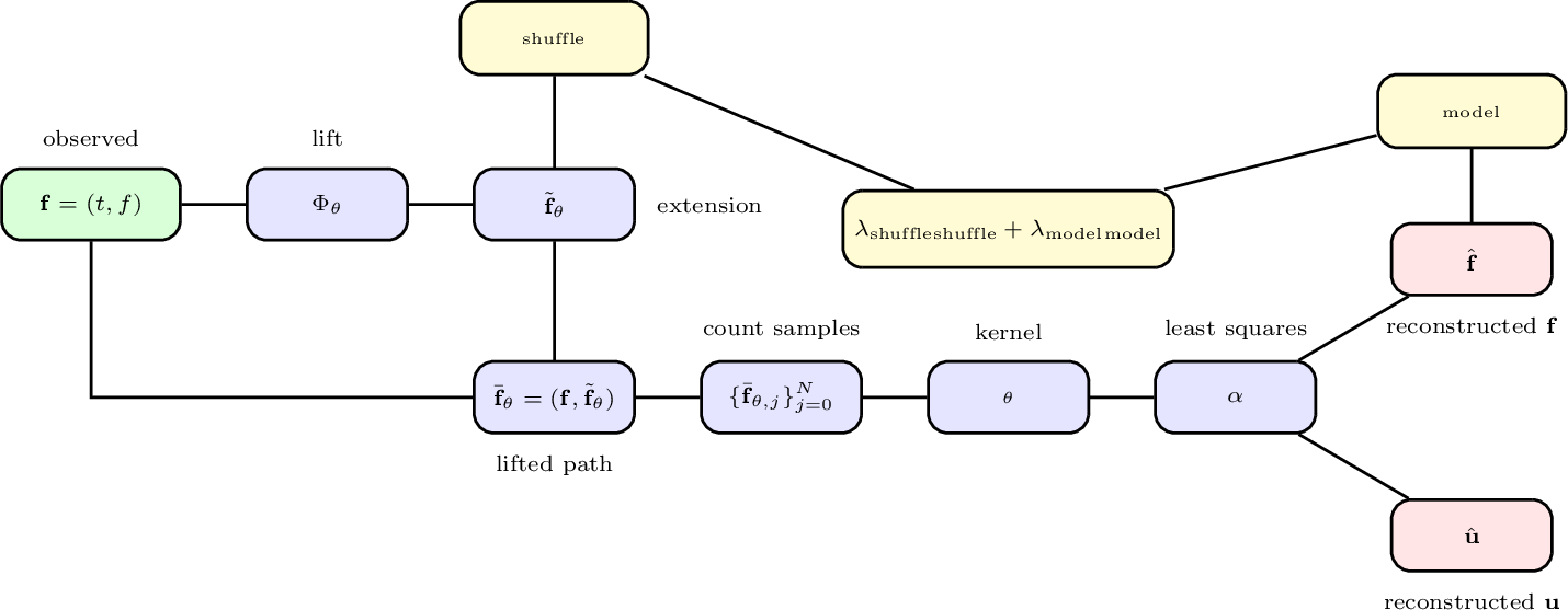
The parameters \(\lambda_{\text{shuffle}}\) and \(\lambda_{\text{model}}\) are tuned so that the model learns an extension which fits the data while still following the branched (non-geometric) signature properties. Often, a higher weight is placed on the model loss than the shuffle loss so that a meaningful extension that actually aids in learning the right representative of the solution of the ODE may be selected. Illustrative diagram of the linear case is presented in Figure 1
5.3.1 Nonlinear Optimizations↩︎
In the case of the nonlinear problem, \(\alpha\) coefficients from the previous iteration are used as a warm start for the next iteration to improve convergence speed. The nonlinear diagram is shown in Figure 2. The computational bottleneck in these models is the \(\alpha\)-optimization step, so we introduce three additional optional hyperparameters to throttle and ramp this
solve. The solve_every parameter freezes the LBFGS updates between calls, reusing the previous \(\alpha\) for a prescribed number of ADAM steps, while the min_iterations and
ramp_portion parameters set a low initial iteration budget and then increase it linearly up to the maximum at a chosen fraction of training. Tuning these parameters helps vastly speed up the initial iterations so that the neural network can
learn expressivity, saving most lfbgs iterations for once the network is expressive. By this point, the warm starts also speed up the final iterations. For highly nonlinear problems, gaps in the frequency of LBFGS solves can cause rapidly spiking model
losses. In these cases, one may opt to simply retrain for \(\alpha\) every iteration and solely employ the ramping-up strategies.
5.3.2 A note on Training Landscape↩︎
Our joint optimization problem trains a neural network to both learning an extension while fitting the constraints of the differential equation. This is in essence the workflow followed by Physics Informed Neural Networks (PINNs). PINNs are well documented for difficulties within the training process. For example, gradient flows of the different loss components are often imbalanced, leading to optimization imbalances [47], [48]. This can be improved through learning rate annealing, network architectures, or gradient normalizations. In our case, specific attention is given to the weighting of shuffle and model loss so that meaningful, nontrivial extensions are learned while sufficient importance is placed on actual model fit. Learning rate schedulers are used when necessary to help re-weight the losses and ensure one does not take over the other. Stiffness and nonlinearity of problems is another essential factor in convergence difficulties [49], [50]. In our cases, we tackle both stiffness and nonlinearity through the use of the RBF signature kernel and tuning of the parameter \(\sigma\). Tuning this parameter gives better fits for highly stiff, oscillatory problems and greatly increases convergence of the L-BFGS optimizer by improving conditioning. However, overtuning this parameter comes at the risk of overfitting the training, leading to poor performance in out of sample predictions. As of now, both the RBF hyperparameters and loss weightings are tuned to address the issues. In future work, one may consider methods introduced in the papers above to stabilize convergence for a wider range of problems.

6 Numerical Experiments↩︎
We test the branched signature kernel solver developed in Section 4 and Section 5 on a range of examples. In particular, we focus on the setting where only a single trajectory of the forcing term is observed, motivated by real-world scenarios in which the forcing signal is typically noisy. We compare the performance of the geometric signature kernel solver and the branched signature kernel solver when the forcing term is highly rough, such as a sample path of fractional Brownian motion. Branched extensions are constructed in the form of the \(t\)-value lift and neural network extension introduced in Definition 27 and Definition 28. These extension methods are compared within experiments, highlighting problems where the T-lift is adequate and demonstrating that in more noisy or complex cases, the neural network extension is needed. Furthermore, both methods from Section 4.1 and Section 4.2 are compared.
Across the experiments, we test and consider variations of the truncation level \(N\) of the signature, kernel matrix normalization (none or robust) and kernel choices (linear or RBF). We note that within each example,
hyper parameters such as regression regularization, L-BFGS tolerance/iteration count, and the RBF sigma value must be tuned correctly. For each section, time lifts are defined by adding a path component of \(t^\alpha\),
where \(\alpha = 2H\) for the holder value H of the underlying generated forcing. The branched neural networks parameters are tuned for each problem for optimal convergence. Each model uses varying hidden depths/layers for
an MLP with a tanh activation function, using Xavier initialization for weights. Integrations of the Kernel Gram Matrices are done using the cumulative trapezoidal integration method unless otherwise stated. Ground truth solutions are generated by either
high order Runge-Kutta integration or implicit multi-step solvers implemented within the scipy library.
6.1 Earthquake displacement model: El-Centro calibration↩︎
We apply the method from Section 4.2 to the 1940 El-Centro strong-motion record sourced from [51]. Structural response is modeled by the damped oscillator, a special case of Example 3: \[\ddot u(t) + 2\xi\omega_n\,\dot{u}(t) + \omega_n^{2}u(t) = -9.81\,a(t), \qquad u(0)=\dot{u}(0)=0,\] where \(a(t)\) is the normalized ground-acceleration record, \(\xi\) is the damping ratio, and \(\omega_n\) is the natural frequency. In the experiment, we take \(\xi=0.02\), \(T_n=5\,\mathrm{s}\), and \(\omega_n=2\pi/T_n\). First calibration is done using a signature depth of 12, a linear kernel, and the robust normalization procedure. Figure 3, displays fits for both the double integrated forcing and solution approximations. The relative MSE for the double integrated forcing was 2.28e-4 while the relative MSE for the solution was 1.47e-04, demonstrating the baseline algorithms effectiveness for moderately rough signals when a high signature depth is used.
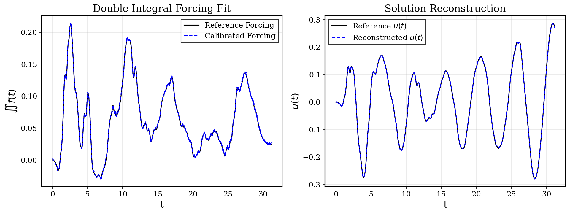
Next, training and testing were applied on a 40/60 split using the rolling-retrain protocol of Section 5, with periodic retraining after 5 predictions. The baseline model is compared to a t-lift model with \(h=.25\) The signature depth is lowered to 5 in order to show the effect of the branched model. The results are summarized in Table 3.
| Training | Testing | |||
|---|---|---|---|---|
| 2-3 (lr)4-5 | Integrated Forcing | Solution | Integrated Forcing | Solution |
| Default Kernel | 4.29e-03 | 4.05e-03 | 1.84e-16 | 1.21e+00 |
| \(t\)-lift branched | 5.68e-04 | 4.63e-04 | 2.53e-21 | 1.19e-01 |
The baseline model fails to accurately predict given the rough signals, while the t-lift greatly improves performance. The t-lift still fails to handle all of the roughness, however, suggesting another extension, such as the neural network may be needed. We note the reason for the testing forcing being fit better than the training forcing is that the training forcing calibrates directly to all of the training data at once, whereas in the rolling retrain, we get new \(\alpha\) values one by one and match them exactly to the new forcing values. We refer to Figure 4 for plots of both models.
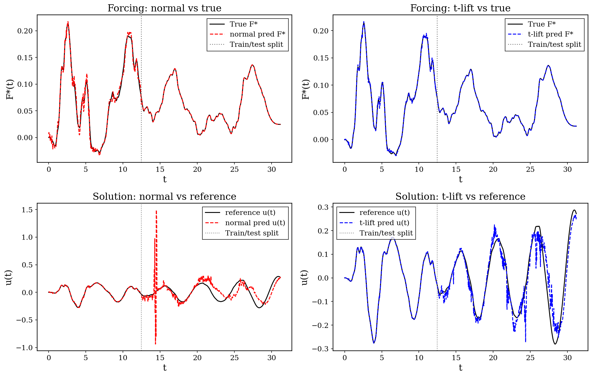
6.2 Solow capital-stock model↩︎
For this example, we use a modified version of the Solow capital-stock growth model [52], where we use real GDP from FRED [53] as the forcing term. The Solow capital-stock dynamics are governed by the first-order linear ODE \[\dot{Y}(t) \;+\; \delta\,Y(t) \;=\; s\,F(t),\qquad Y(0)=Y_0,\] with depreciation rate \(\delta\in[0,1]\), savings rate \(s\in[0,1]\), GDP forcing \(F(t)\), and initial capital stock \(Y_0>0\). In the notation of Definition 32, this is the \(d=1\), \(m=1\) instance with \(A_1=1\), \(A_0=\delta\), forcing \(sF(t)\), and initial data \(g_0=Y_0\). In our experiment, we set an initial condition \(Y_0=3.1\). We apply the linear integral method of Section 4.2 with no normalization and signature truncation level \(N=3\). First consider the results of calibration on the entire interval, shown in Figure 5. The relative integrated forcing and solution errors were 6.59e-08 and 1.14e-06 respectively. The lower truncation level here reflects the smoother, first-order nature of the Solow ODE in comparsion to the el-centro problem, allowing for lower level signatures to capture the dynamics.
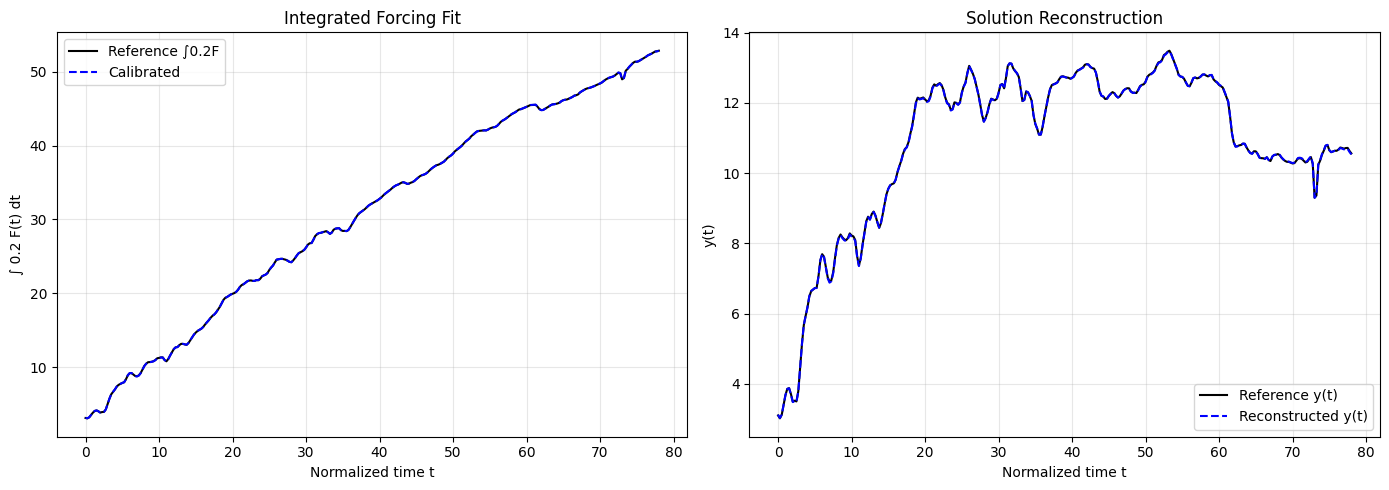
Next, a testing and training experiment is done using the rolling retrain protocol, using the same hyperparameters as before. The first 50 data points are used for training, with periodic retraining applied every 10 steps. The results in Figure 6 and Table 4 confirm the low depth signatures capabilities in this case.
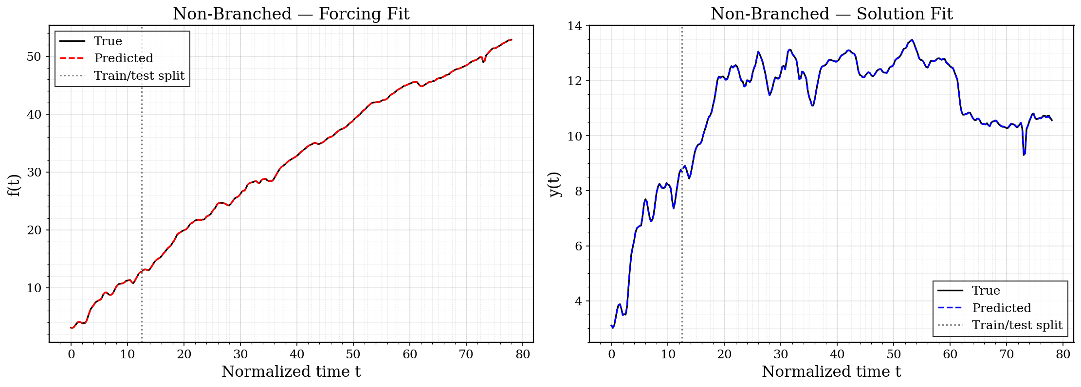
| Training | Testing | |
|---|---|---|
| Forcing | 2.91e-9 | 6.53e-29 |
| Solution | 1.91e-06 | 1.04e-06 |
6.3 Linear ODE with fBM Forcing Example↩︎
Consider a linear second order ODE (SDOF equation) driven by a fractional Brownian motion forcing term. We use the following governing equation. \[m\ddot{U} + c\dot{U} + k U = F(t), \qquad U(0) =a, \quad U'(0) =b,\] In our simulation, \(F(t)\) is a 3000 point fBM on the interval from 0 to 1 with hurst parameter \(H=.25\). \(m,c,\) and \(k\) are set at 1, 10, and 5 respectively. We compare training and prediction performance across the baseline signature model, t-lift, and neural lift models, also comparing across methods from Section 4.1 and Section 4.2, refered to as method 1 and method 2, respectively. For each method, an RBF signature kernel with signature depth 3 and \(\sigma=1\) is employed along with the robust normalization method. The standard training and prediction method are applied to a 90/10 test train split, with periodic retraining every 2 steps. For our neural lift, 3 extensions are trained with hidden depths \((2, 4, 8, 4, 2)\) over 1500 ADAM epochs. Overall learning rate, model loss weight, and shuffle loss weight were set to be 5e-3, 10, and 1e-4 respectively, with a learning rate scheduler reducing losses for every 300 stale iterations.
We first refer to Table 5 for comparisons of the methods. The first method vastly outperforms the second, likely due to the double integration of the forcing introducing approximation errors. The second method also fails to predict well, showing inconsistent results. For problems with such rough forcings or higher orders of integrations required, it is therefore recommended to use Method 1.
| Method 1 | Method 2 | |||||
|---|---|---|---|---|---|---|
| 2-4 (lr)5-7 | Baseline | \(t\)-lift | Branched | Baseline | \(t\)-lift | Branched |
| Training Solution | 4.56e-11 | 2.15e-11 | 1.22e-11 | 1.12e-06 | 2.68e-07 | 5.46e-09 |
| Testing Solution | 4.76e-09 | 3.18e-11 | 1.17e-13 | 6.24e-03 | 6.01e-03 | 3.55e-02 |
Next, we compare the results of Method 1 on the calibration and prediction task. Results are shown in Table 6. Across the training and testing sections, both branched models outperform the baseline model. The neural network extension performs magnitudes better than the t lift in calibration, and performs better in predicting the solution as well. This suggests the neural branched model is able to sufficiently capture the branched structure within the rough paths. We refer to Figure 7 for results of the neural model on testing and prediction.
| Training | Testing | |||
|---|---|---|---|---|
| 2-3 (lr)4-5 | Forcing | Solution | Forcing | Solution |
| Baseline | 1.89e-04 | 4.56e-11 | 1.96e-01 | 4.76e-09 |
| t-lift Solution | 2.57e-05 | 2.15e-11 | 3.32e-03 | 3.18e-11 |
| Branched Solution | 3.36e-07 | 1.22e-11 | 8.91e-03 | 1.17e-13 |
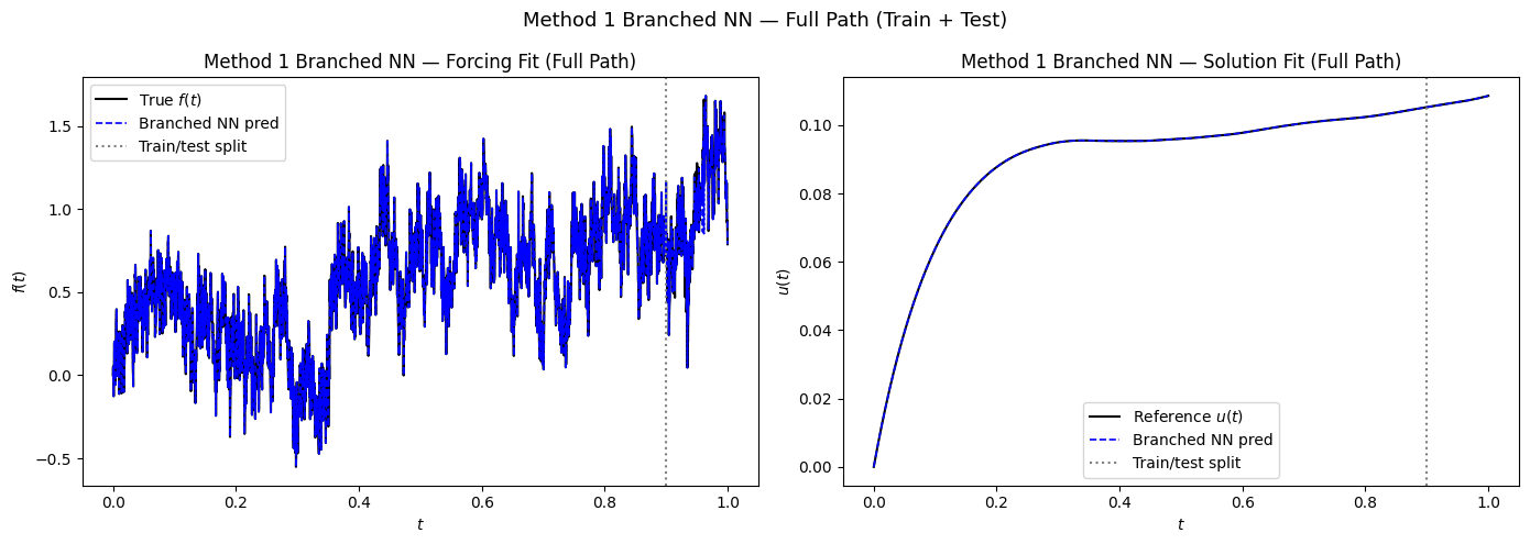
6.4 Modeling Nonlinear ODE driven by FBM (Duffing Model)↩︎
The Duffing oscillator extends the second-order SDOF system with a nonlinear cubic term and has broad applications across many fields. It is used to model nonlinear vibrations in timber structures [54], energy harvesting under magnetic forcing and its noisy extensions [55], [56], financial asset dynamics with fractional Gaussian processes [57], and complex signal processing in high-noise environments [58]. Duffing oscillators driven by Gaussian noise are also employed for stochastic resonance and weak-signal detection, including mechanical fault diagnosis such as rolling bearing and rotor faults [59], [60], and have been further developed within stochastic modeling frameworks [61].
We apply our branched signature kernel method to solve Duffing oscillators of the standard form with Neumann and Dirichlet boundary conditions as specified in Example 35 using the nonlinear approximation method described in 4.3. Our time values consist of 3000 points over the interval 0 to 1. We set \(a=0, b=1, k_0=5, k_1=10, \gamma=10\) as our constants and coefficients. The forcing is taken as a fractional Brownian motion with hurst parameter \(H=.25\). The first 90 percent of values are used for training while testing is done on the last 10 percent. A signature depth of 3 is used together with column-wise robust normalization. The kernel is chosen to be radial basis with bandwidth \(\sigma=3\). The standard prediction procedure is used, with retraining performed every 2 steps. The maximum LBFGS iteration is set to 300. The branched architecture employs hidden layer widths \((2, 4, 8, 4, 2)\) and learns 2 extension channels. Optimization proceeds using ADAM for 2000 iterations with learning rate \(3e-4\) consisting of model loss weight \(10\) and shuffle loss weight \(10e-3\). We use the acceleration procedures from 5.3.1, solving for \(\alpha\) every 100 ADAM iterations while ramping up from 50 to 300 LFBGS iterations over the first 25 percent of ADAM iterations.
The results for both the baseline and branched model are summarized in Table 7. While both models fit extremely well in and out of sample, the branched model showed significant improvement over the baseline signature kernel model. This demonstrates the neural networks ability to encode the branched information not captured by the classical signature. The results for the branched models testing and training fits are presented in Figure 8
| Training | Testing | |||
|---|---|---|---|---|
| 2-3 (lr)4-5 | Forcing | Solution | Forcing | Solution |
| Non-branched | 4.60e-02 | 7.86e-05 | 4.88e-03 | 9.31e-08 |
| Branched | 1.80e-02 | 1.66e-05 | 3.42e-03 | 4.79e-08 |
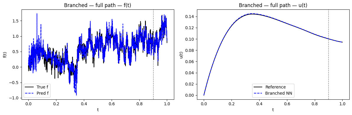
6.5 Variable Coefficient ODE: Arias-Intensity degraded SDOF↩︎
We have considered the case of linear ODEs with constant coefficients. However, we may also examine equations in which the coefficients depend on the time or forcing themselves.
36 (Variable Coefficient Second Order Linear ODE). \[\begin{align} \color{red} &k_1(t,f(t)) u''(t) + k_2(t,f(t)) u'(t) + k_3(t,f(t)) u(t)=f(t), \quad u(0)=a,\quad u'(0)=b, \end{align}\] with functions \(k_1,k_2,k_3\) and \(x\in[0,T]\).
Forms of the SDOF system with time-varying coefficients have been studied in [62]–[64]. As long as the coefficients do not depend on \(u(t)\) or its derivatives, the ODE reamins linear and the signature-kernel algorithm is unchanged: one simply evaluates the coefficient functions on the grid when forming the alphas and kernel matrix ansatz. Our solver therefore applies directly to ODEs with path-dependent coefficients. We illustrate this with an example from earthquake engineering. The Arias intensity [65] \[I_A(t)\;:=\;\frac{\pi}{2g}\int_{0}^{t}a(s)^{2}\,\mathrm{d}s\] is a path functional of the ground acceleration that quantifies the cumulative energy delivered to the structure. Given a damage source \(D(t)\), effective stiffness is often modeled as decaying with damage [66]: \[k_{eff}(t) = (1-D(t))k_0, \qquad \frac{k_{eff}(t)}{m} = \frac{(1-D(t))k_0}{m} = (1-D(t))\omega_0^2.\]
As the Arias intensity strongly correlates with destructive potential [67], we introduce a degradation rate \(\delta\) and use \(I_A(t)\) as the damage variable, yielding the variable stiffness coefficient \[A_0(t)=\omega_n^{\,2}\bigl(1-\delta\,I_A(t)\bigr)_{+},\] where \((\cdot)_{+}:=\max(\cdot,0)\) enforces non-negative stiffness. Substituting this into Definition 36 gives the Arias-intensity degraded SDOF model:
37 (Arias-intensity degraded SDOF). \[\ddot u(t) \;+\; 2\xi\omega_n\,\dot{u}(t) \;+\; A_0(t)\,u(t) \;=\; -9.81\,a(t), \qquad u(0)=0,\quad \dot{u}(0)=0,\] with degradation rate \(\delta\ge 0\). The coefficient \(A_0(t)\) depends on the forcing path through the cumulative integral \(I_A(t)\).
In the collocation framework of 7 , the block matrix becomes \[L_{ji} \;=\; A_2\,K_{ji} \;+\; A_1\,K^{(1)}_{ji} \;+\; A_0(t_j)\,K^{(2)}_{ji},\] where \(I_A(t_j)=\tfrac{\pi}{2g}\sum_{k=0}^{j-1}a(t_k)^{2}(t_{k+1}-t_k)\) is computed once from the count-sampled forcing path \(\boldsymbol{f}_j=(a(t_0),\ldots,a(t_j))\). The integral method and calibration protocol of Section 4.1 and Section 5 remain unchanged.
For the experiment, calibration is compared across the baseline and branched signature kernel models, along with a solver using a point-wise rbf kernel with no signatures. We consider an example in which the acceleration \(a(t)\) is given by a fractional brownian motion with hurst parameter \(H=.2\). We set \(\omega_n = 2\pi, \xi = .05, \delta = 5\). 1000 observations are taken over the interval from 0 to 1. Refer to Figure 9 for plots of the forcing, Arias intensity, and effective stiffness coefficient.
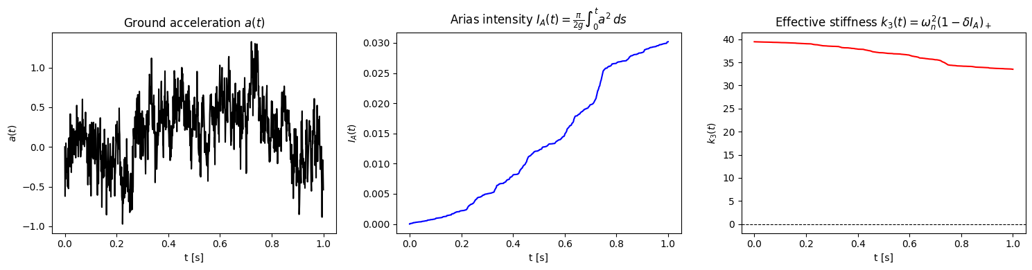
For each case, a radial basis kernel with \(\sigma=1\) is used. Signature solvers use a signature depth of 2 together with a column‑wise robust normalization. The branched model trains 3 extensions using hidden layers \((4, 8, 16, 8, 4, 2)\). Optimization is done for 2000 epochs, employing the ADAM algorithm with learning rate \(10e-4\), a model loss weighted by 10, and a shuffle regularization term weighted by \(10e-4\). A plateau-based learning rate schedule reduces the step size by a factor of 0.5 after 500 epochs without improvement. The results for the three models are summarized in Table 8 and plotted in Figure 10.
| Model | Forcing | Solution |
|---|---|---|
| RBF (No Signatures) Kernel Model | \(5.49\mathrm{e}{-1}\) | \(1.17\mathrm{e}{-3}\) |
| Non-branched Signature Kernel Model | \(2.94\mathrm{e}{-4}\) | \(1.46\mathrm{e}{-8}\) |
| Branched Signature Kernel Model | \(\mathbf{6.34\mathrm{e}{-6}}\) | \(\mathbf{3.37\mathrm{e}{-11}}\) |
The base RBF Kernel fails to adequately model the rough forcing term and misses some of the shaping within the solution. The base signature model sees better results, but is unable to capture all of the branched information within the forcing path. The Branched Model shows the best performance out of all models by significant orders of magnitudes. We note that for the point-wise RBF model, the \(\sigma\) parameter may be "over-tuned", i.e. shrunk extremely small so that the kernel matches the forcing’s roughness. However, this overfitting leads to a complete inability to predict out of sample. The branched signature kernel model remains able to fit both the forcing and predict out of sample without overfitting to the data, as seen in Example 6.4
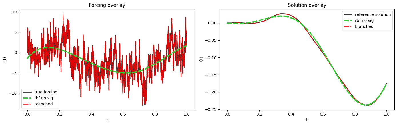
6.6 Noisy Kuramoto oscillator system↩︎
The general Kuramoto oscillator system [68] on \(n\) coupled phase oscillators is given by \[\frac{d\theta_i}{dt} \;=\; \omega_i + \frac{1}{n}\sum_{j=1}^{n} K_{ij}\, \sin(\theta_j - \theta_i), \qquad i = 1, \ldots, n, \label{eq:kuramoto}\tag{28}\] where \(\theta_i(t) \in \mathbb{T}\) is the phase of oscillator \(i\), \(\omega_i \in \mathbb{R}\) its natural frequency, and \(K_{ij} \in \mathbb{R}\) the coupling strength. Here \(n\) is the number of oscillators, distinct from the count-sampled path count \(N\) used elsewhere. Introducing a uniform coupling constant \(K\) and additive white noise \(\zeta_i\) yields the noisy system [69], which can be written either as an ODE or in differential form: \[\frac{d\theta_i}{dt} = \omega_i + \zeta_i + \frac{K}{n}\sum_{j=1}^{n} \sin(\theta_j - \theta_i) \qquad\text{or}\qquad d\theta_i(t) = \Bigl[ \omega_i + \frac{K}{n}\sum_{j=1}^{n} \sin(\theta_j - \theta_i) \Bigr] dt + d B_i^H(t),\] where \(B_i^H(t)\) is a fractional Brownian motion with hurst parameter \(H\). We may write its ODE form as: \[\frac{d\theta_i}{dt} = \omega_i + \frac{K}{n}\sum_{j=1}^{n} \sin(\theta_j - \theta_i) + \zeta_i(t),\quad \text{or}\quad \frac{d\theta_i}{dt} - \omega_i - \frac{K}{n}\sum_{j=1}^{n} \sin(\theta_j - \theta_i) = \zeta_i(t).\]
In the first form, one could observe the right-hand side and use the signature-kernel algorithm to calibrate it and recover \(\theta\), a linear task in which the branched signature captures the fractional Gaussian noise. Here we instead analyze the second form: we observe the noise and use the nonlinear approximation algorithm to calibrate the left-hand side to the right, enforcing the physical law.
First, let us describe how to generate the required data and reference solution. We fix \(n\), frequencies \(\omega_i\) for \(i=1,\dots,n\), and coupling constant \(K\), choose a uniform grid \(0 = t_0, \dots, t_{N-1} = T\), and set the initial phase vector \(\theta(0)=\bigl(\theta_1(0),\ldots,\theta_n(0)\bigr)\). For each oscillator \(i\), we generate a fractional Brownian motion sample path \(B_i^H(t_0), \dots, B_i^H(t_{N-1})\) with Hurst parameter \(H\). Using increments \(\Delta B_i^H(t_k):=B_i^H(t_{k+1})-B_i^H(t_k)\) and time step \(\Delta t=t_{k+1}-t_k\), \(k = 0,\dots,N-2\), we construct the Euler approximation \[\theta_i(t_{k+1}) = \theta_i(t_k) + \Bigl[ \omega_i + \frac{K}{n}\sum_{j=1}^{n}\sin\bigl(\theta_j(t_k)-\theta_i(t_k)\bigr) \Bigr]\Delta t + \Delta B_i^H(t_k),\] for \(k = 0,\dots,N-2\) and \(i = 1,\dots,n\). For the signature-kernel solver via 4.1, we take the raw path and fractional Gaussian noise approximated by \[\mathbf{f}_k = \bigl(t_k,\eta_1^H(t_k),\eta_2^H(t_k),\ldots,\eta_n^H(t_k)\bigr), \qquad \eta_i^H(t_k) \approx \frac{\Delta B_i^H(t_k)}{\Delta t}.\]
For our simulation, we set \(n=3\) oscillators with frequencies of \(-1, -.3\), and \(1.5\), respectively. The coupling constant is set to \(k=3\). Each oscillator is driven by a \(3000\) point fractional Brownian motion with Hurst parameter \(H=0.4\). Initial values of \(\theta\) are selected randomly along the range \([0,2\pi)\). Signature depth for the models is set at 3, and robust normalization is used along with an RBF kernel with parameter \(\sigma=1\) and LBFGS iteration count of 400. For this example, trapezoid integration is replaced by a left point Reimann sum as to be consistent with the generation scheme. The branched model trains 2 extensions with hidden layers \((8, 16, 32, 16, 8)\). Optimization is done with 1000 ADAM iterations with an overall learning rate of \(3e-4\), model loss weight of \(1e3\), and shuffle loss weight of \(1e-3\). The model loss is set higher in this case to compensate for the contribution of all 3 generated paths to the shuffle loss. Acceleration is applied through the methods in 5.3.1. Due to the highly nonlinear sine term causing spikes in losses, we choose to optimize for \(\alpha\) at every ADAM iteration. LFBGS Iterations start off at 20 and linearly ramp up to the maximum of 400 at 75 percent of the iterations.
Results showing fits of the models for the forcing, derivative of the solution, and solution for the branched and non branched models are presented in Table 9. Plots of the branched model fits for each oscillators forcing and solution are presented in Figure 11. Both models fit all oscillators extremely well. However, the branched model shows superior performance in all categories, once again demonstrating its ability to encode information within the branched signature.
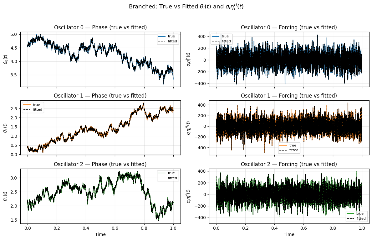
| Model | Forcing | \(d\theta / dt\) | \(\theta\) |
|---|---|---|---|
| Non-branched Signature Kernel Model | \(1.73\mathrm{e}{-6}\) | \(1.73\mathrm{e}{-6}\) | \(1.78\mathrm{e}{-7}\) |
| Branched Signature Kernel Model | \(\mathbf{5.25\mathrm{e}{-15}}\) | \(\mathbf{1.31\mathrm{e}{-11}}\) | \(\mathbf{1.33\mathrm{e}{-8}}\) |
Acknowledgements↩︎
References↩︎
KSig: Gpu-accelerated computation of the signature kernel. arXiv preprint
arXiv:2501.07145.