Point-group symmetry analysis of many-electron wavefunctions on a quantum computer
May 24, 2026
Abstract
A point group is a set of spatial symmetry operations in molecular systems and is an indispensable tool for analyzing molecular orbitals and spectroscopy experiments in chemistry. Several quantum algorithms to exploit this symmetry have been proposed,
but practical implementations of point-group symmetry operations and the detailed symmetry analysis of realistic many-electron wavefunctions are still missing. In this work, we propose an ancilla-free hybrid method to analyze point-group symmetries of
many-electron states, which works for both abelian and non-abelian groups. For a given wavefunction, our method calculates the projection weights of point-group irreducible representations by applying orbital rotations derived from the eigenvectors of the
representation matrices, therefore it is applicable to arbitrary basis functions. The usefulness of our approach is demonstrated through numerical simulations of benzene and ferrocene molecules. Furthermore, we perform a hardware demonstration of the
weight calculation of the ground state and the first excited state of benzene in \(D_{2h}\) symmetry, using up to 32 qubits of IBM’s ibm_kawasaki device. By combining a tensor-network based encoding scheme and
error mitigation techniques, we find the weights of irreducible representations for both states are faithfully reproduced within a few percent error. Our results suggest that the proposed method serves as a practical tool for analyzing symmetry properties
of many-electron wavefunctions in realistic material simulations on near-term and early fault-tolerant quantum computers.
1 introduction↩︎
Symmetry is a fundamental concept in quantum mechanics, and quantum computing algorithms significantly benefit from considering symmetries of a given system. For example, the conservation of the total electron number in the molecular electronic structure Hamiltonian, related to \(U(1)\) symmetry [1], leads to a simplified circuit ansatz [2] or a reduction in the number of qubits [3]. Therefore, finding and utilizing symmetries of a given quantum state is crucially important for realizing quantum simulations on near-term devices and early fault-tolerant quantum computers.
A point group [4] is a finite group of spatial symmetry operations in molecular systems and is widely used in theoretical and experimental chemistry. It also plays key roles in understanding intriguing physical phenomena and chemical reactions, such as the Jahn-Teller effect [5]–[7] and the Woodward-Hoffmann rules [8]. Quantum algorithms have also been proposed to exploit this symmetry [9]–[11]. One of the most useful applications of point group symmetry is the symmetry-adapted projection of many-electron wavefunctions [12]–[14]; by projecting a general many-electron state onto a specific irreducible representation of the point group, this operation allows for obtaining not only the ground state but also excited states of the system. However, while the general methodology of symmetry-adapted projection has been discussed, a concrete implementation of point group symmetry operations and the analysis of symmetry properties of realistic many-electron wavefunctions remain largely underexplored.
In this work, we aim to bridge this gap by presenting a practical framework for analyzing point group symmetry properties of realistic many-electron wavefunctions. For this purpose, we focus on calculating the weights of irreducible representations in a given wavefunction as a tool to analyze its symmetry properties. We propose an ancilla-free, quantum-classical hybrid method to calculate this quantity, which works for both abelian and non-abelian point groups. This method leverages the fact that, under the Jordan-Wigner transformation, point group symmetry operations can be implemented on a quantum circuit with \(O(1)\) depth for commonly used symmetry-adapted molecular orbitals (e.g. Hartree-Fock orbitals) and with \(O(n)\) depth for general orbitals, where \(n\) is the number of spatial orbitals.
The usefulness of this approach is showcased through numerical simulations of two prototype molecules, benzene and ferrocene. To be specific, through a detailed analysis of single Slater determinants and local unitary cluster Jastrow functions [15], we show that our method yields practical information about the point-group symmetries of many-electron wavefunctions, and that it is also useful for assessing the quality of given trial wavefunctions.
Furthermore, as a proof of concept calculation, we present a hardware demonstration of calculating the weights of irreducible representations for benzene in \(D_{2h}\) symmetry, using up to 32 physical qubits of IBM’s
superconducting quantum device ibm_kawasaki. We prepare the ground-state and the first excited-state wavefunctions of this molecule with density matrix renormalization theory (DMRG) [16], [17], and use a tensor-network based technique similar to Ref. [18] to classically convert them into a brick-wall ansatz. We note that for the DMRG wavefunctions expressed in a matrix
product state (MPS) form, the same calculation can be done classically using matrix product operators (MPO) [17]. However, we emphasize
that our approach can be applied to arbitrary many-electron quantum states, including strongly-correlated states or time-evolved states that cannot be described efficiently in tensor-network based methods.
To extract ideal noise-free results, we compare two error mitigation techniques: (i) zero noise extrapolation (ZNE) [19] with gate-folding implemented in Qiskit [20], and (ii) quasi-probabilistic error mitigation approach implemented in QESEM [21], [22]. Our demonstration shows that the proposed approach is useful not only for symmetry analysis of a given many-electron wavefunction, but also for benchmarking real quantum devices and error mitigation techniques.
The rest of the paper is organized as follows. Section 2 outlines point group symmetry and explains our proposed algorithm. Section 3 provides numerical simulations for benzene and ferrocene. Section 4 presents a hardware demonstration of the proposed method on IBM’s quantum hardware. Conclusions are drawn in Sec. 5.
2 theory↩︎
2.1 Finite group and projection operator↩︎
First we consider a general finite symmetry group \(G\). The projection of a general quantum state \(|\Psi\rangle\) onto one of its irreducible representations \(\Gamma\) is [4], [12], [13] \[P_{\Gamma} |\Psi\rangle = \frac{d_{\Gamma}}{|G|} \sum_{C} \chi^{*}_{\Gamma}(C) \sum_{g \in C} \hat{g} |\Psi\rangle, \label{eq:p95gamma}\tag{1}\] where \(d_{\Gamma}\) is the dimension of \(\Gamma\), \(|G|\) is the order of \(G\), \(C\) is a conjugacy class with \(\chi_{\Gamma}(C)\) its character in \(\Gamma\), and \(\hat{g}\) is a symmetry group operation acting on \(|\Psi\rangle\). The state \(|\Psi\rangle\) is projected onto \(\Gamma\) as \[P_{\Gamma}|\Psi\rangle = a_{\Gamma} |\Psi_{\Gamma}\rangle,\] where \(|\Psi_{\Gamma}\rangle\) is a superposition of the basis functions of irreducible representation \(\Gamma\), and \(a_{\Gamma}\) is its coefficient. These states are orthonormalized as \(\langle \Psi_{\Gamma}|\Psi_{\Gamma'}\rangle=\delta_{\Gamma \Gamma'}\), therefore \(\sum_{\Gamma} |a_{\Gamma}|^{2} = 1\). Note that \(P_{\Gamma}\) in Eq. (1 ) is related to a more general operator [4] \[P_{\Gamma,jj'} = \frac{d_{\Gamma}}{|G|} \sum_{g} \bigl[ D_{\Gamma}(g)\bigr]^{*}_{jj'} \hat{g} \quad j,j'=1,2,\dots,d_{\Gamma}, \label{eq:p95gamma95gen}\tag{2}\] where \(D_{\Gamma}(g)\) is the irreducible representation matrix for \(g\) in \(\Gamma\), which is related to \(\chi_{\Gamma}(C)\) as \(\chi_{\Gamma}(C) = \textrm{Tr} D_{\Gamma}(g \in C)\). It can be shown that the state \(|\Psi_{\Gamma,jj'}\rangle = P_{\Gamma,jj'}|\Psi\rangle\) behaves as a \(j\)-th symmetry-adapted basis function of \(\Gamma\) [4].
The central quantity in this paper is the weight of \(\Gamma\), defined as \(w_{\Gamma} = |a_{\Gamma}|^{2}\). This quantity characterizes symmetric properties of the input state \(|\Psi\rangle\), and may be viewed as the power spectrum of the generalized Fourier transform associated with finite group \(G\) [13], [23]. Using Eq. (1 ), \(w_{\Gamma}\) is calculated as \[\begin{align} w_{\Gamma} &=& \langle \Psi |P_{\Gamma}|\Psi\rangle \nonumber\\ &=& \frac{d_{\Gamma}}{|G|} \sum_{C} \chi_{\Gamma}^{*}(C) \sum_{g \in C} \langle \Psi | \hat{g}|\Psi\rangle. \label{eq:w95gamma} \end{align}\tag{3}\] In Appendix, we show that in the above expression \(\sum_{\Gamma} w_{\Gamma} = 1\) is guaranteed as long as \(\langle \Psi |\Psi \rangle = 1\).
2.2 Point group in quantum chemistry↩︎
A point group is a fundamental finite symmetry group of a molecule, and is used to classify its molecular orbitals and electronic states in quantum chemistry. By operating a point-group symmetry element \(\hat{g}\), a general set of one-particle orbitals \(\{\phi_{\nu \sigma}\}\) transform as \[\hat{g} \phi_{\nu \sigma} = \sum_{\mu = 1}^{n} \bigl[ D(g) \bigr]_{\mu\nu} \phi_{\mu \sigma}, \label{eq:g95psi95general}\tag{4}\] where \(D(g)\) is the unitary representation matrix of \(g\) with respect to \(\{ \phi_{\nu\sigma}\}\), \(\mu\) and \(\nu\) are spatial orbital indices, and \(\sigma\in \{\uparrow, \downarrow\}\) is a spin index. We restrict ourselves to the spin-restricted case (i.e., \(\phi_{\nu \uparrow} = \phi_{\nu \downarrow}\)); the generalization to the spin-unrestricted case is straightforward.
In practical calculations, the representation matrices \[\bigl[ D(g)\bigr]_{\mu \nu} = \langle \phi_{\mu \sigma} |\hat{g}|\phi_{\nu \sigma}\rangle\] need to be prepared. When the orbitals are expanded by some basis functions \(\{\mathcal{B}_{I}\}\) as \(\phi_{\nu \sigma} = \sum_{I} x_{I \nu \sigma} \mathcal{B}_{I}\), the matrix elements of \(D(g)\) are calculated as \[\bigl[ D(g)\bigr]_{\mu \nu} = \sum_{IJK} x^{*}_{I \mu \sigma} \mathcal{S}_{IJ} \Bigl[D^{(B)}(g)\Bigr]_{JK} x_{K \nu \sigma},\] where \(\mathcal{S}_{IJ} = \langle \mathcal{B}_{I}|\mathcal{B}_{J}\rangle\) and \(D^{(B)}(g)\) are the overlap and the representation matrices for \(\{\mathcal{B}_{I}\}\), respectively.
When \(\{\phi_{\nu \sigma}\}\) are chosen to be the solution of a one-particle Hamiltonian having the point group symmetry of the system, each degenerate set of orbitals form the basis functions of an irreducible representation of the point group. Examples of such mean-field-like Hamiltonians include the Fock operator in the Hartree-Fock approximation [24] and the Kohn-Sham Hamiltonian in density functional theory [25]. The \(\gamma\)-th set of degenerate orbitals \(S_{\gamma \sigma}=\{\psi_{\gamma j \sigma}\} (j=1,2,\dots,|S_{\gamma \sigma}|)\) hybridize exclusively with one another, as \[\hat{g} \psi_{\gamma k \sigma} = \sum_{j=1}^{|S_{\gamma \sigma}|} \bigl[ \bar{D}_{\gamma} (g) \bigr]_{j k} \psi_{\gamma j \sigma}. \label{eq:g95psi95irrep}\tag{5}\] In this case \(D(g)\) in Eq. (4 ) can be written in a block-diagonal form, and the size of \(\bar{D}_{\gamma}(g)\) in Eq. (5 ) is \(O(1)\) for simple monomer molecules considered in this work.
Many-electron wavefunctions are expanded by a tensor product of one-particle orthonormal wavefunctions \[\sum_{\sigma_{1}\sigma_{2}\dots}\sum_{\nu_{1}\nu_{2}\dots} C^{\sigma_{1}\sigma_{2}\dots}_{\nu_{1} \nu_{2} \dots} \phi_{\nu_{1}\sigma_{1}}\phi_{\nu_{2}\sigma_{2}} \dots,\] and the reducible representation of \(g\) with respect to these tensor product basis states is obtained as \[\begin{align} \hat{g} \phi_{\nu_{1}\sigma_{1}}\phi_{\nu_{2}\sigma_{2}} \dots &=& \sum_{\mu_{1} \mu_{2}\dots} \bigl[ D(g) \bigr]_{\mu_{1} \nu_{1}} \bigl[ D(g) \bigr]_{\mu_{2} \nu_{2}} \dots \nonumber\\ && \qquad \phi_{\mu_{1}\sigma_{1}} \phi_{\mu_{2}\sigma_{2}} \dots \label{eq:g95manybody} \end{align}\tag{6}\]
2.3 Point group symmetry operations on a quantum computer↩︎
As discussed by Yen et al. [12], a point-group symmetry operation on many-electron states, \(\hat{g} |\Psi \rangle = U(g) |\Psi \rangle\), corresponding to Eq. (6 ), is expressed as an orbital rotation \[\begin{align} U(g) &=& \prod_{\sigma} U^{\sigma}(g), \\ U^{\sigma}(g) &=& \exp \Bigl[\sum_{\mu,\nu=1}^{n} \bigl[ \log D(g)\bigr]_{\mu \nu} c^{\dagger}_{\mu \sigma} c_{\nu \sigma} \Bigr]. \label{eq:ug} \end{align}\tag{7}\] Here \(c^{\dagger}_{\mu \sigma}\) and \(c_{\nu \sigma}\) are electron creation and annihilation operators, respectively, and \(D(g)\) is defined in Eq. (4 ). Under the Jordan-Wigner transformation, this rotation can be implemented using the Givens rotations [26] with \(O(n)\) depth for general orbitals (Eq. (4 )). For symmetry-adapted, mean-field orbitals (Eq. (5 )), the depth is reduced to \(O(1)\) by decomposing \(U^{\sigma}(g)\) as \[U^{\sigma}(g) = \prod_{\gamma} U^{\sigma}_{\gamma}(g), \label{eq:ug95ug95gamma}\tag{8}\] where \[U^{\sigma}_{\gamma}(g) = \exp \Bigl[\sum_{j,k = 1}^{|S_{\gamma \sigma}|} \bigl[ \log \bar{D}_{\gamma}(g)\bigr]_{j k} c^{\dagger}_{\gamma j \sigma} c_{\gamma k \sigma} \Bigr] \label{eq:ug95gamma}\tag{9}\] with \(\bar{D}_{\gamma}(g)\) defined in Eq. (5 ).
Using these operators, the projection operation (Eq. (1 )) is implemented using the linear combination of unitary (LCU) technique [27]. The standard LCU requires \(\lceil \log_{2} |G| \rceil\) ancilla qubits, and a single-ancilla LCU approach [28] is also proposed for evaluating expectation values of observables.
2.4 Weight evaluation on a quantum computer↩︎
Here we consider a quantum-classical hybrid approach to calculate \(w_{\Gamma}\) defined in Eq. (3 ), which evaluates \(\langle \Psi | \hat{g} |\Psi \rangle = \langle \Psi | U(g) |\Psi \rangle\) for each \(g\) on a quantum computer and post-processes the results to construct \(w_{\Gamma}\). As discussed in Appendix, \(\sum_{\Gamma} w_{\Gamma} = 1\) is ensured even in noisy simulations, provided that \(\langle \Psi |U(E)|\Psi\rangle = \langle \Psi|\Psi\rangle = 1\) is given exactly. It should be noted that \(w_{\Gamma}\) can be evaluated in a fully quantum way by, for example, measuring ancilla qubits in the generalized symmetry-adapted transform (GSA) proposed in Ref. [13], but these coherent approaches require a deeper circuit with multiply controlled operations.
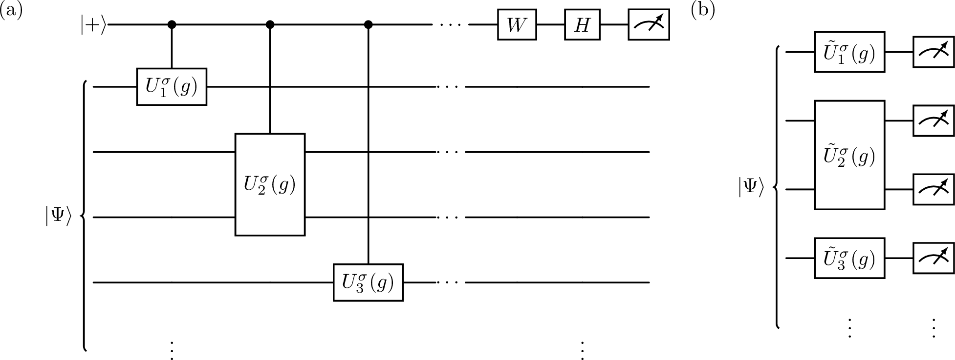
One way to evaluate \(\langle \Psi | U(g) | \Psi \rangle\) is the Hadamard test using one ancilla qubit, as shown in Fig. 1 (a). This approach, however, requires \(O(n)\) long-range controlled \(U^{\sigma}_{\gamma}(g)\) operations, therefore it is not suitable for quantum devices with limited qubit connectivity.
To circumvent this difficulty, we propose an ancilla-free method shown in Fig. 1 (b). This method is based on the diagonalization of each \(\bar{D}_{\gamma}(g)\) \[\bar{D}_{\gamma}(g) = V^{g}_{\gamma} \textrm{diag}\Bigl[ e^{i \varphi^{g}_{\gamma 1}},e^{i \varphi^{g}_{\gamma 2}}, \dots \Bigr] V^{g \dagger}_{\gamma},\] and rewrites \(U^{\sigma}_{\gamma}(g)\) as \[U^{\sigma}_{\gamma}(g) = \bigl(\tilde{U}^{\sigma}_{\gamma}(g)\bigr)^{\dagger} \Bigl[ \prod_{k} e^{i \varphi^{g}_{\gamma k} \tilde{c}_{\gamma k \sigma}^{\dagger} \tilde{c}_{\gamma k \sigma}} \Bigr] \tilde{U}^{\sigma}_{\gamma}(g). \label{eq:ugnu}\tag{10}\] Here \(\tilde{U}^{\sigma}_{\gamma}(g)\) is an orbital rotation \[\tilde{U}^{\sigma}_{\gamma}(g) = \exp \Bigl[ \sum_{jk} \bigl[\log V^{g \dagger}_{\gamma} \bigr]_{jk} c_{\gamma j \sigma}^{\dagger} c_{\gamma k \sigma}\Bigr], \label{eq:tilde95ugnu}\tag{11}\] and \[\tilde{c}^{\dagger}_{\gamma k \sigma} = \sum_{j} \bigl[V^{g}_{\gamma}\bigr]_{j k} c^{\dagger}_{\gamma j \sigma}.\] As \(\prod_{k} e^{i \varphi^{g}_{\gamma k} \tilde{c}^{\dagger}_{\gamma k \sigma} \tilde{c}_{\gamma k \sigma}}\) in Eq. (10 ) is diagonal in the computational basis, \(\langle \Psi |U(g)|\Psi \rangle\) can be obtained by measuring \(|\tilde{\Psi}(g)\rangle = \prod_{\sigma} \prod_{\gamma} \tilde{U}^{\sigma}_{\gamma}(g) |\Psi\rangle\) and combining the results with appropriate phase factors. We note that the qubit tapering technique proposed in Ref. [9] employs a similar methodology for abelian groups. Our approach can also be used for non-abelian groups and for general orbitals (Eq. (4 )) with \(O(n)\) depth overhead for the orbital rotation.
Next we discuss the sample complexity of the method. Noting \[\textrm{Var} \Bigl[ \prod_{\sigma}\prod_{\gamma}\prod_{k} e^{i \varphi_{\gamma k}^{g} \tilde{c}^{\dagger}_{\gamma k \sigma} \tilde{c}_{\gamma k \sigma}} \Bigr] \leq 1,\] the number of total measurements \(M\) for a given total variance \(\epsilon^{2}\) is bounded as [29] \[M \leq \frac{1}{\epsilon^{2}} \Bigl( \sum_{C} \frac{r_{C}}{|G|} |\chi_{\Gamma}(C)| \Bigr)^{2}, \label{eq:m}\tag{12}\] where \(r_{C}\) is defined in Eq. (22 ). Using the orthonormality of \(\chi_{\Gamma}(C)\) (Eq. (20 )) and the Cauchy-Schwarz inequality, Eq. (12 ) becomes \[M \leq \frac{1}{\epsilon^{2}} \Bigl(\sum_{C}r_{C} \cdot \frac{|\chi_{\Gamma}(C)|^{2}}{|G|^{2}}\Bigr) \cdot \Bigl(\sum_{C} r_{C} \cdot 1^{2} \Bigr) = \frac{1}{\epsilon^{2}},\] which indicates that the number of measurements required is independent of \(|G|\) and \(\Gamma\).
For abelian groups, all irreducible representations are one-dimensional. In this case \(\tilde{U}_{\gamma}(g) = I\) for all \(g \in G\), therefore all \(U(g)\) can be measured simultaneously. Furthermore, when \(\bar{D}_{\gamma}(g) = \pm 1\) for all \(g\), \(\langle \Psi |U(g)|\Psi \rangle\) can be obtained by calculating the expectation value of a single Pauli operator \(P(g) = \prod_{\sigma} \prod_{\gamma} P_{\gamma}(g)\), where \[P_{\gamma}(g) = \left\{ \begin{array}{ll} I & \quad \bar{D}_{\gamma}(g) = 1 \\ Z & \quad \bar{D}_{\gamma}(g) = -1 . \end{array} \right.\]
3 Numerical simulations on a classical computer↩︎
| \(D_{6h}\) | \(E\) | \(2 C_{6}\) | \(2C_{3}\) | \(C_{2}''\) | \(3C_{2}\) | \(3C_{2}'\) | \(\sigma_{h}\) | \(3 \sigma_{v}\) | \(3 \sigma_{d}\) | \(2S_{6}\) | \(2 S_{3}\) | \(i\) |
|---|---|---|---|---|---|---|---|---|---|---|---|---|
| \(A_{1g}\) | +1 | +1 | +1 | +1 | +1 | +1 | +1 | +1 | +1 | +1 | +1 | +1 |
| \(A_{1u}\) | +1 | +1 | +1 | +1 | +1 | +1 | -1 | -1 | -1 | -1 | -1 | -1 |
| \(A_{2g}\) | +1 | +1 | +1 | +1 | -1 | -1 | +1 | -1 | -1 | +1 | +1 | +1 |
| \(A_{2u}\) | +1 | +1 | +1 | +1 | -1 | -1 | -1 | +1 | +1 | -1 | -1 | -1 |
| \(B_{1g}\) | +1 | -1 | +1 | -1 | +1 | -1 | -1 | -1 | +1 | +1 | -1 | +1 |
| \(B_{1u}\) | +1 | -1 | +1 | -1 | +1 | -1 | +1 | +1 | -1 | -1 | +1 | -1 |
| \(B_{2g}\) | +1 | -1 | +1 | -1 | -1 | +1 | -1 | +1 | -1 | +1 | -1 | +1 |
| \(B_{2u}\) | +1 | -1 | +1 | -1 | -1 | +1 | +1 | -1 | +1 | -1 | +1 | -1 |
| \(E_{1g}\) | +2 | +1 | -1 | -2 | 0 | 0 | -2 | 0 | 0 | -1 | +1 | +2 |
| \(E_{1u}\) | +2 | +1 | -1 | -2 | 0 | 0 | +2 | 0 | 0 | +1 | -1 | -2 |
| \(E_{2g}\) | +2 | -1 | -1 | +2 | 0 | 0 | +2 | 0 | 0 | -1 | -1 | +2 |
| \(E_{2u}\) | +2 | -1 | -1 | +2 | 0 | 0 | -2 | 0 | 0 | +1 | +1 | -2 |
| \(D_{5d}\) | \(E\) | \(2C_{5}\) | \(2C_{5}^{2}\) | 5\(C_{2}'\) | \(i\) | \(2S_{10}^{3}\) | \(2S_{10}\) | \(5\sigma_{d}\) |
|---|---|---|---|---|---|---|---|---|
| \(A_{1g}\) | +1 | +1 | +1 | +1 | +1 | +1 | +1 | +1 |
| \(A_{1u}\) | +1 | +1 | +1 | +1 | -1 | -1 | -1 | -1 |
| \(A_{2g}\) | +1 | +1 | +1 | -1 | +1 | -1 | +1 | -1 |
| \(A_{2u}\) | +1 | +1 | +1 | -1 | -1 | -1 | -1 | +1 |
| \(E_{1g}\) | +2 | \(+x_{+}\) | \(+x_{-}\) | 0 | +2 | \(+x_{+}\) | \(+x_{-}\) | 0 |
| \(E_{1u}\) | +2 | \(+x_{+}\) | \(+x_{-}\) | 0 | -2 | \(-x_{+}\) | \(-x_{-}\) | 0 |
| \(E_{2g}\) | +2 | \(+x_{-}\) | \(+x_{+}\) | 0 | +2 | \(+x_{-}\) | \(+x_{+}\) | 0 |
| \(E_{2u}\) | +2 | \(+x_{-}\) | \(+x_{+}\) | 0 | -2 | \(-x_{-}\) | \(-x_{+}\) | +1 |
For a better understanding of point-group symmetry properties of many-electron wavefunctions, we present classical simulations on two prototype molecules, benzene (C\(_{6}\)H\(_{6}\)) and staggered ferrocene (FeC\(_{10}\)H\(_{10}\)) [30], [31], which belong to \(D_{6h}\) and \(D_{5d}\) point groups, respectively. The character tables of these two point groups are shown in Tables 1 and 2.
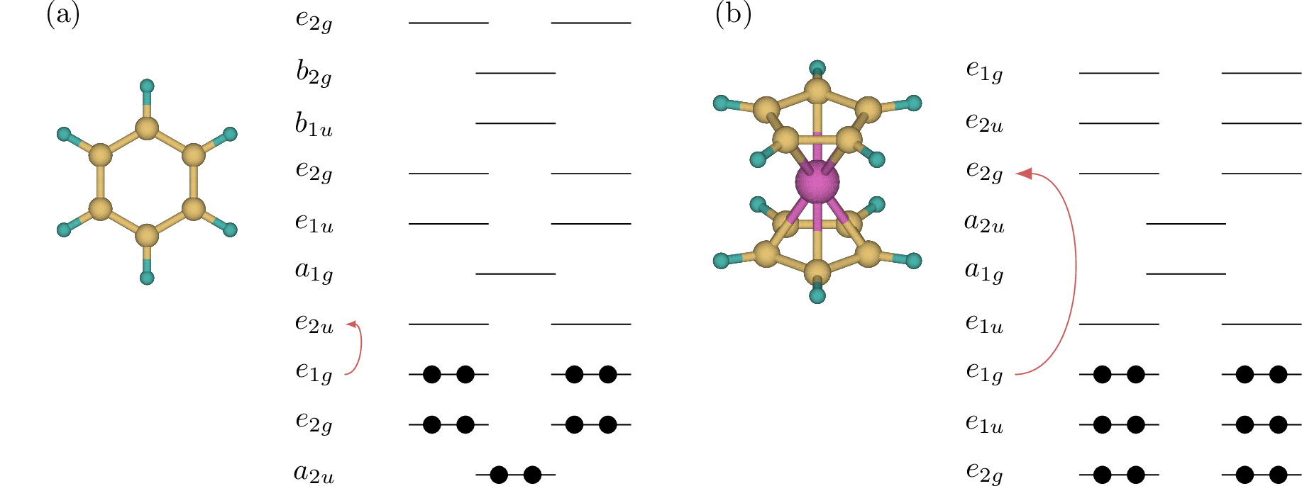
The calculations are conducted using ffsim [32], [33], and the Hamiltonian and the representation matrix elements are calculated using pyscf [34] with 6-31G basis. The bond lengths of benzene used are 1.39 Å and 1.09 Å for C-C and C-H bonds, respectively. The structure of the staggered ferrocene is taken from Ref. [31]. The active spaces of benzene and ferrocene are chosen as (10e,16o) and (12e,16o), respectively. Here, (\(m\)e,\(n\)o) denotes a space spanned by \(m\) electrons in \(n\) spatial orbitals. The structures and the Hartree-Fock one-particle energy diagrams of the two molecules are shown in Fig. 2, together with the irreducible representation labels (in lowercase) of the orbitals.
3.1 Single Slater determinant case↩︎
We start with the case where the wavefunction is expressed as a single Slater determinant \[|\Psi\rangle = \prod_{\sigma \in \{\uparrow, \downarrow\}} \prod_{\mu_{\sigma}=1}^{n_{\sigma}} c^{\dagger}_{p_{\mu_{\sigma}} \sigma} |0\rangle,\] where \(n_{\sigma}\) is the number of electrons in a spin state \(\sigma\), and \(\{p_{\mu_{\sigma}}\}\) denote occupied orbitals. In this case \(\langle\Psi| U(g) |\Psi\rangle\) is easily calculated as \[\langle\Psi| U(g) |\Psi\rangle = \prod_{\sigma \in \{\uparrow, \downarrow\}} \textrm{det} \mathcal{D}_{\sigma}(g), \label{eq:ug95sd}\tag{13}\] where \(\mathcal{D}_{\sigma}(g)\) is an \(n_{\sigma} \times n_{\sigma}\) matrix whose matrix elements are defined as \[\bigl[ \mathcal{D}_{\sigma}(g)\bigr]_{\mu_{\sigma} \nu_{\sigma}} = \bigl[D(g)\bigr]_{p_{\mu_{\sigma}} p_{\nu_{\sigma}}}.\]
We calculate the weights \(w_{\Gamma}\) for the Hartree-Fock ground states and single excited (SE) states of the two molecules. This calculation is inspired by the work in Ref. [35], where the reduction of point-group representations formed from many-electron wavefunctions in benzene and xenon tetrafluoride (XeF\(_4\)) is carried out. The Hartree-Fock ground-state configurations are \((a_{2u})^{2}(e_{2g})^{4}(e_{1g})^{4}\) and \((e_{2g})^{4}(e_{1u})^{4}(e_{1g})^{4}\) for benzene and ferrocene, respectively (see Fig. 2). The SE configurations considered are \((a_{2u})^{2}(e_{2g})^{4}(e_{1g})^{3}(e_{2u})^{1}\) and \((e_{2g})^{4}(e_{1u})^{4}(e_{1g})^{3} (e_{2g})^{1}\), respectively, as indicated by the arrows in Fig. 2. For each molecule, there are eight independent SE configurations with \(S_{z}=0\), where \(S_{z}\) is the \(z\)-component of the total spin.
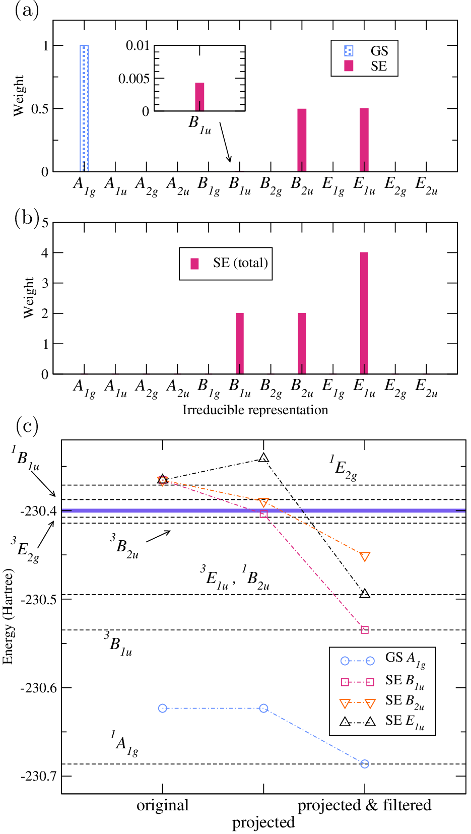
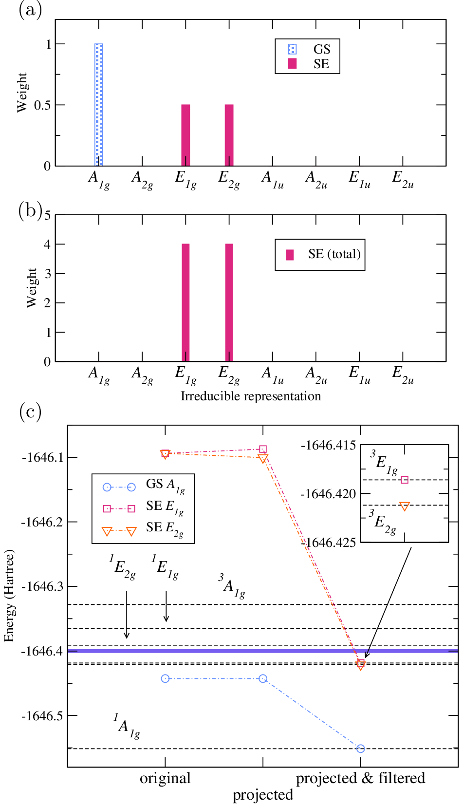
The calculated weights for benzene and ferrocene are plotted in Fig. 3 (a) and Fig. 4 (a), respectively. For the SE states, the results of one configuration (out of eight) are shown for each molecule. The Hartree-Fock ground states of both molecules belong to the perfectly symmetric \(A_{1g}\) irreducible representation, as expected for any closed shell configuration [35]. On the other hand, the SE states in both molecules consist of multiple irreducible representations. For benzene, shown in Fig. 3 (a), the chosen SE state is decomposed as \(\approx 0.005 B_{1u} + 0.495 B_{2u} + 0.5 E_{1u}\). Note that in this partially-filled configuration these values are dependent on the details of the diagonalization routine used in the Hartree-Fock calculation, as they are not invariant with respect to the unitary transformation of the degenerate orbitals \[\psi_{\gamma k \sigma} \to \psi'_{\gamma k \sigma} = \sum_{j} V^{\gamma}_{jk} \psi_{\gamma j \sigma} \label{eq:u95trans}\tag{14}\] with \(V^{\gamma}_{j k}\) an arbitrary unitary matrix.
The reduction of the eight-dimensional representation for the SE states, similar to Ref. [35], can be done by summing the weights for all the eight SE configurations, namely, by calculating \[\begin{align} w^{\textrm{SE-total}}_{\Gamma} &=& \sum_{i \in \textrm{SE}} w^{(i)}_{\Gamma}\nonumber\\ &=& \frac{d_{\Gamma}}{|G|} \sum_{C} \chi^{*}_{\Gamma}(C) \sum_{g\in C} \nonumber\\ && \qquad \sum_{i \in \textrm{SE}} \langle \Psi^{(i)}|U(g)|\Psi^{(i)}\rangle . \label{eq:w95se95total} \end{align}\tag{15}\] Here \(|\Psi^{(i)}\rangle\) is the \(i\)-th SE configuration. Note that \(\sum_{i \in \textrm{SE}} \langle \Psi^{(i)}|U(g)|\Psi^{(i)}\rangle\) corresponds to the character of the (reducible) representation for the SE states, and Eq. (15 ) coincides with the well-known formula for counting the number of occurrences of \(\Gamma\) in a given representation [35], up to a prefactor of \(d_{\Gamma}\). As can be seen in Fig. 3 (b), this eight-dimensional space in benzene is decomposed as \(2 B_{1u} + 2 B_{2u} + 4 E_{1u}\), and this result is invariant with respect to the orbital transformation (Eq. (14 )). Similarly, one SE configuration of ferrocene is decomposed as \(0.5 E_{1g} + 0.5 E_{2g}\), and the total eight-dimensional SE space is decomposed as \(4 E_{1g} + 4 E_{2g}\), as shown in Fig. 4 (b).
To investigate the effect of the symmetry projection (Eq. (1 )), in Fig. 3 (c) and Fig. 4 (c) the energy expectation values of the following three wavefunction sets are calculated for the two molecules:
the original Hartree-Fock ground state and one SE state.
states obtained by applying the symmetry projection \(P_{\Gamma}\) to
states obtained by applying an energy-based filter to 2.
We apply a step-function like filter with cutoff energy as \(\Theta (H - E_{\textrm{cutoff}}) |\Psi\rangle\), where \[\Theta (E) = \left\{ \begin{array}{ll} 1 & E < 0 \\ 0 & E > 0. \end{array} \right.\] This filter can be implemented, for example, with the quantum eigenvalue transformation of unitary matrices (QETU) [36]. In Fig. 3 (c) and Fig. 4 (c), the cutoff energy and the exact eigenstates are shown by thick and dashed lines, respectively.
In both cases, applying the symmetry projection to the Hartree-Fock ground state does not decrease the energy, as the state already belongs to the correct irreducible representation (\(A_{1g}\)) of the ground state. For the SE states, their energy expectation values after the symmetry projection are also higher than the lowest exact eigenstates with the same irreducible representations. By applying the filter, the exact eigenenergies are obtained for all the projected states except the SE state for benzene projected onto \(B_{2u}\) (Fig. 3 (c)). The reason for this discrepancy is that there are two eigenstates below the cutoff belonging to \(B_{2u}\) but with different spin (\(^{1}B_{2u}\) and \(^{3}B_{2u}\)); this example shows the limitation of the current procedure.
This simple numerical experiment confirms that the symmetry projection (Eq. (1 )) is useful to get exact eigenstates with specific irreducible representations, but it has to be combined with other algorithms, such as filtering [36], quantum phase estimation [37], or spin projection [12]. Our proposed method provides a simple yet powerful tool for analyzing symmetries of a trial wavefunction before performing the projection.
3.2 Interacting case: local unitary cluster Jastrow function↩︎
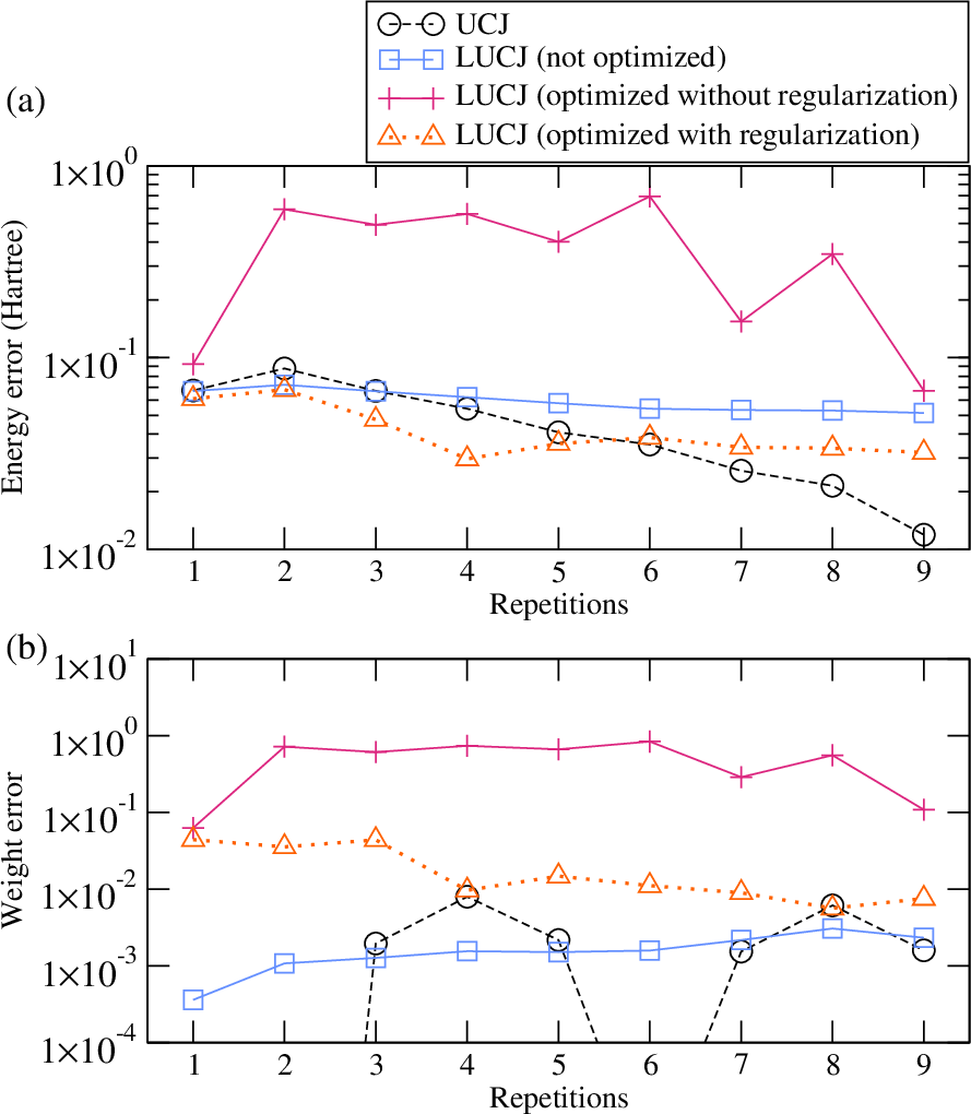
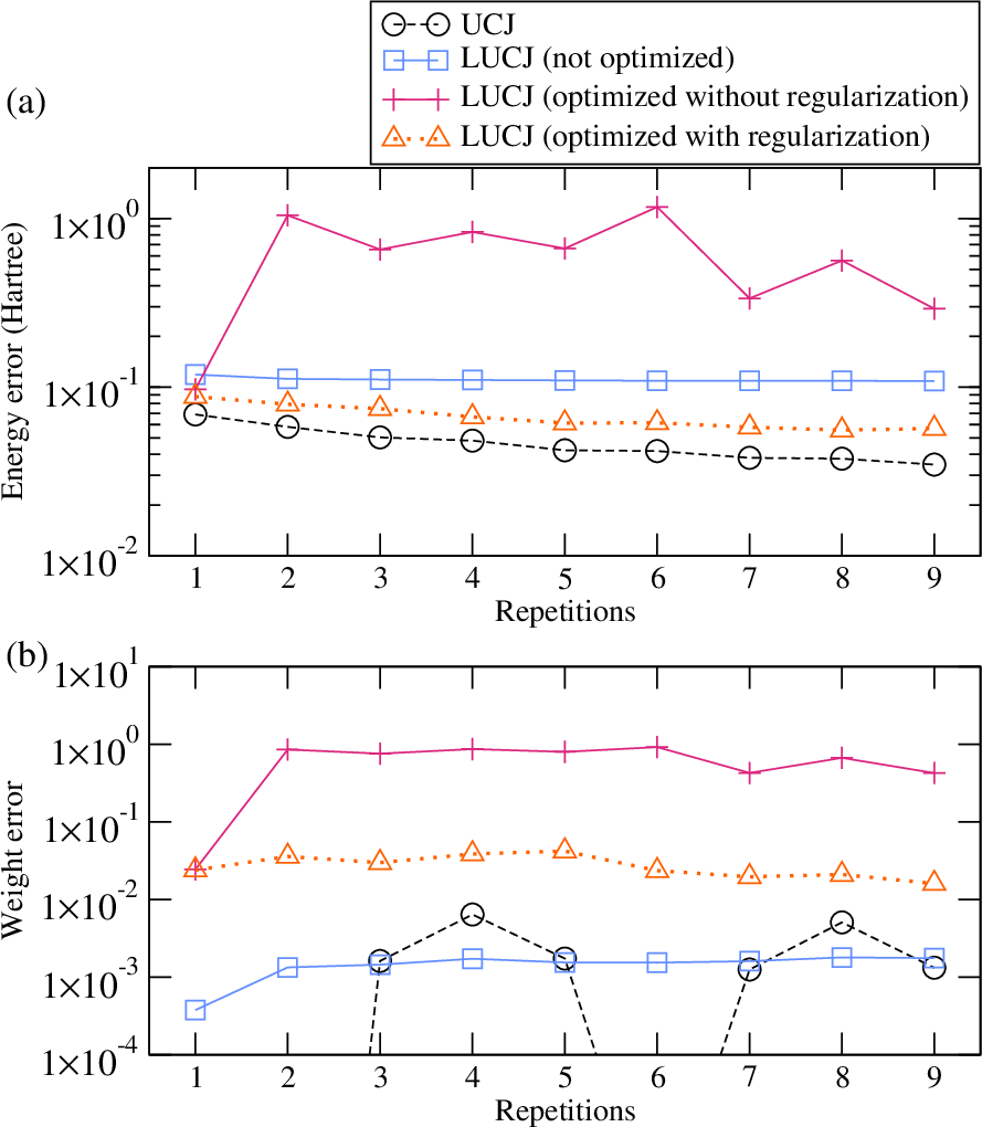
As an example of correlated wavefunctions, we next present a symmetry analysis of the unitary cluster Jastrow (UCJ) function and its local variant known as the local unitary cluster Jastrow (LUCJ) function [15]. These wavefunctions are proposed as an approximation of the unitary coupled-cluster wavefunction, and are often used as a trial state of the sample-based quantum diagonalization [38].
The UCJ wavefunction has the form [15], [38], [39] \[|\Psi\rangle = \prod_{r=1}^{R} \mathcal{U}_{r} e^{i \mathcal{J}_{r}} \mathcal{U}_{r}^{\dagger} |\Psi_{\textrm{0}}\rangle,\] where \(|\Psi_{\textrm{0}}\rangle\) is a reference state which we take as the Hartree-Fock ground state, \(\mathcal{U}_{r}\) is an orbital rotation, \(R\) is the number of repetitions, and \(\mathcal{J}_{r}\) is a density-density interaction operator \[\mathcal{J}_{r} = \frac{1}{2} \sum_{\sigma,\sigma'}\sum_{\mu,\nu} J^{(r)\sigma \sigma'}_{\mu \nu} n_{\mu \sigma} n_{\nu \sigma'} \label{eq:j}\tag{16}\] with \(n_{\mu\sigma} = c^{\dagger}_{\mu \sigma} c_{\mu \sigma}\).
The LUCJ wavefunction is obtained by retaining only selected terms in Eq. (16 ) that are compatible with a specific qubit connectivity. For the heavy-hexagonal connectivity considered in this work, \(J^{(r)\sigma \sigma'}_{\mu \nu}\) is allowed to be nonzero only for the following orbital sets: \[\begin{align} S_{\sigma = \sigma'} &=& \{(p, p+1)| p=1,2,\dots,n - 1\} \\ S_{\sigma \neq \sigma'} &=& \{(p, p)| p=1, 5, 9,\dots, n\}. \end{align}\]
The parameters in the (L)UCJ wavefunctions are often initialized using the truncated double-factorized form of the \(t_{2}\) amplitudes obtained from a classical coupled-cluster singles and doubles (CCSD) calculation [38], [39] \[t_{oo' uu'} \approx i \sum_{r=1}^{R}\sum_{\mu\nu} J^{(r)}_{\mu\nu} U_{u\mu}^{(r)}U_{o\mu}^{(r)*}U_{u'\nu}^{(r)}U_{o'\nu}^{(r)*}.\] Here \(o\) and \(o'\) (\(u\) and \(u'\)) denote occupied (unoccupied) orbitals, \(J^{(r)}\) is a real symmetric matrix used in the interaction operator (Eq. (16 )), and \(U^{(r)}\) is a unitary matrix for an orbital rotation.
In Ref. [39], two methods are proposed to optimize the parameters in the (L)UCJ functions, and we focus on their first method. This method optimizes the sparsified interaction matrices \(\bar{J}^{(r)}\) due to connectivity restriction and the corresponding rotation matrices \(\bar{U}^{(r)}\) by minimizing \[\frac{1}{2}\sum_{oo'uu'} |\bar{t}_{oo'uu'} - t_{oo'uu'}|^{2} + \lambda \Bigl| \sum_{r} || \bar{J}^{(r)}||_{\textrm{F}}^{2} - \sum_{r} || J^{(r)}||_{\textrm{F}}^{2} \Bigr|. \label{eq:min95j}\tag{17}\] Here \(\bar{t}_{oo'uu'}\) are compressed \(t_{2}\) amplitudes [39] constructed from \(\bar{J}^{(r)}\) and \(\bar{U}^{(r)}\), and the subscript \(\textrm{F}\) denotes the Frobenius norm. The second term in Eq. (17 ) is a regularization term used to prevent one term from becoming too large.
Our objective here is to investigate the point-group symmetry properties of the UCJ and LUCJ functions and see the effect of the optimization procedure described above. We prepare the (L)UCJ functions for benzene and ferrocene using ffsim [32], [33], and calculate the energy expectation value and also the weight of \(A_{1g}\), which is the irreducible representation of the exact ground state.
The calculated results as a function of repetitions \(R\) are plotted in Fig. 5 and Fig. 6 for benzene and ferrocene, respectively. For the LUCJ functions, we compare three parameter sets: (i) unoptimized (initialized with the CCSD \(t_{2}\) amplitudes), (ii) optimized without regularization, and (iii) optimized with regularization parameter \(\lambda = 0.005\) [39]. For comparison, the results for the UCJ function without parameter optimization are also plotted.
As also reported in Ref. [39], in both systems the optimized LUCJ wavefunction without regularization results in the largest energy error. The error in the weight of \(A_{1g}\) for this wavefunction is also significantly large in most cases, indicating that the optimization through Eq. (17 ) does not preserve the symmetry of the reference wavefunction. For the other three wavefunctions, the discrepancy is smaller. Perhaps not surprisingly, the UCJ and unoptimized LUCJ wavefunctions provide very high (\(>99\)%) \(A_{1g}\) weights, as the \(t_{2}\) amplitudes in CCSD reflect the symmetries of the orbitals. It can also be seen that the optimized LUCJ wavefunction with regularization yields a smaller \(A_{1g}\) weight than the unoptimized LUCJ, but it improves the energy expectation value. This indicates that having a higher weight of the correct irreducible representation does not guarantee a higher-quality approximation.
In Ref. [39], it is also reported that when used as a trial state for the sample-based energy estimation with quantum-selected configuration interaction (QSCI) [40], the (L)UCJ function optimized without regularization yields a lower energy than those optimized with regularization. Our symmetry analysis suggests that for sample-based approaches using broken-symmetry wavefunctions could enhance the efficiency of sample-based approaches.
4 Demonstration on real quantum hardware↩︎
| Date | April 29, 2026 |
| Number of qubits | 156 |
| Processor type | Heron r2 |
| Basis gates | cz,id,rx,rz,rzz,sx,x |
| Median readout error | 5.49\(\times 10^{-3}\) |
| Median cz error | 1.677\(\times 10^{-3}\) |
| Median sx error | 1.973\(\times 10^{-4}\) |
| Median \(T_{1}\) (\(\mu\)s) | 307.34 |
| Median \(T_{2}\) (\(\mu\)s) | 157.38 |
| \(D_{2h}\) | \(E\) | \(C_{2}\) | \(C_{2}'\) | \(C_{2}''\) | \(i\) | \(\sigma_{h}\) | \(\sigma_{v}\) | \(\sigma_{d}\) |
|---|---|---|---|---|---|---|---|---|
| \(A_{g}\) | +1 | +1 | +1 | +1 | +1 | +1 | +1 | +1 |
| \(A_{u}\) | +1 | +1 | +1 | +1 | -1 | -1 | -1 | -1 |
| \(B_{1g}\) | +1 | +1 | -1 | -1 | +1 | +1 | -1 | -1 |
| \(B_{1u}\) | +1 | +1 | -1 | -1 | -1 | -1 | +1 | +1 |
| \(B_{2g}\) | +1 | -1 | -1 | +1 | +1 | -1 | +1 | -1 |
| \(B_{2u}\) | +1 | -1 | -1 | +1 | -1 | +1 | -1 | +1 |
| \(B_{3g}\) | +1 | -1 | +1 | -1 | +1 | -1 | -1 | +1 |
| \(B_{3u}\) | +1 | -1 | +1 | -1 | -1 | +1 | +1 | -1 |
| \(D_{6h}\) | \(A_{1g}\) | \(A_{1u}\) | \(A_{2g}\) | \(A_{2u}\) | \(B_{1g}\) | \(B_{1u}\) | \(B_{2g}\) | \(B_{2u}\) | \(E_{1g}\) | \(E_{1u}\) | \(E_{2g}\) | \(E_{2u}\) |
|---|---|---|---|---|---|---|---|---|---|---|---|---|
| \(D_{2h}\) | \(A_{g}\) | \(A_{u}\) | \(B_{1g}\) | \(B_{1u}\) | \(B_{2g}\) | \(B_{2u}\) | \(B_{3g}\) | \(B_{3u}\) | \(B_{2g}+B_{3g}\) | \(B_{2u}+B_{3u}\) | \(A_{g}+B_{1g}\) | \(A_{u}+B_{1u}\) |
In this section, we demonstrate the evaluation of the weights \(w_{\Gamma}\) in Eq. (3 ) on IBM’s superconducting quantum device ibm_kawasaki for the ground state and the first
excited state of benzene. The specifications of the device are summarized in Table 3.
We consider three active spaces, (10e,8o), (10e,12o), and (10e,16o) with the Jordan-Wigner encoding, corresponding to 16, 24, and 32 qubits, respectively. For simplicity, we assume abelian \(D_{2h}\) point group (Table 4) instead of \(D_{6h}\). In this reduced point group, the irreducible representations of \(D_{6h}\) transform according to Table 5. We calculate the Hartree-Fock orbitals of benzene, used as the encoding basis, with imposing \(D_{2h}\) symmetry.
We employ the Pauli-based evaluation method explained in Sec. 2.3; each \(\langle \Psi |U(g)|\Psi\rangle\) is evaluated as the expectation value of a single Pauli operator \(P(g)\). In the case of \(D_{2h}\), there are eight mutually commuting Pauli operators, including one identity operation.
4.1 Compression of DMRG wavefunctions↩︎
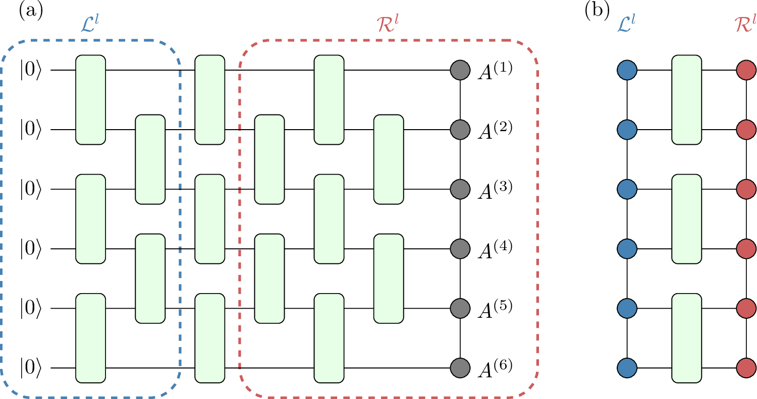
Similarly to Ref. [18], we prepare trial wavefunctions from classical DMRG calculations and convert them into a brick-wall ansatz for approximate circuit encoding. After the Jordan-Wigner transformation, the DMRG wavefunction of \(2n\) spin orbitals is written in an MPS form \[\begin{align} |\Psi_{\textrm{DMRG}}\rangle &=& \sum_{\sigma_{1},\sigma_{2},\dots,\sigma_{2n}} \sum_{m_{2},m_{3},\dots,m_{2n}} \nonumber\\ && A^{(1)}_{m_{1} \sigma_{1} m_{2}} A^{(2)}_{m_{2} \sigma_{2} m_{3}} \dots A^{(2n)}_{m_{2n} \sigma_{2n} m_{2n+1}} \nonumber\\ &&\times|\sigma_{1}\sigma_{2}\dots\sigma_{2n}\rangle, \label{eq:mps} \end{align}\tag{18}\] with \(m_{1}=m_{2n+1}=1\). Here \(\sigma_{p}\) and \(m_{p}\) \((p=1,2,\dots,2n)\) denote physical spin and virtual bond indices, respectively, and \(A^{(p)}_{m_{p}\sigma_{p}m_{p+1}}\) in this work is right-normalized as \[\sum_{\sigma_{p} m_{p+1}} A^{(p) *}_{m_{p}\sigma_{p} m_{p + 1}} A^{(p)}_{m'_{p}\sigma_{p} m_{p + 1}} = \delta_{m_{p} m'_{p}}.\] This wavefunction is encoded in a quantum circuit using a brick-wall ansatz with \(L\) layers \[|\tilde{\Psi}\rangle = \prod_{l=1}^{L} \prod_{b=1}^{B_{l}} U_{l b} | 0 \rangle^{\otimes 2 n},\] where \(U_{l b}\) is a two-qubit unitary, and \(B_{l}\) is the number of \(U_{l b}\) in layer \(l\) \[B_{l} = \left\{ \begin{array}{ll} n & \textrm{odd} \,\, l \\ n-1 & \textrm{even} \,\, l . \end{array} \right.\]
We optimize \(U_{lb}\) iteratively using a scheme similar to Ref. [18]; we introduce the cost function \[\begin{align} \mathcal{C} &=& \bigl|\bigl| \,|\Psi_{\textrm{DMRG}}\rangle - |\tilde{\Psi}\rangle \bigr|\bigr|^{2} \nonumber\\ &=& 2 - 2 \textrm{Re} \langle \Psi_{\textrm{DMRG}}|\tilde{\Psi}\rangle, \label{eq:cost95bw95mps} \end{align}\tag{19}\] and perform a layer-by-layer optimization. As schematically shown in Fig. 7, to optimize \(U_{lb}\) in layer \(l\), two auxiliary MPSs \(\mathcal{L}^{l}\) and \(\mathcal{R}^{l}\) are prepared. The “left” MPS \(\mathcal{L}^{l}\) is calculated by operating \(U_{l' b}\) on \(| 0 \rangle^{\otimes 2n}\) sequentially for \(l'=1,2,\dots,l-1\), and converting the resulting state into an MPS form in each step via the singular value decomposition (SVD) [17], [41]. Similarly, the “right” MPS \(\mathcal{R}^{l}\) is calculated by applying \(U^{\dagger}_{l' b}\) in reverse order, for \(l'=L, L-1, \dots, l+1\) to \(|\Psi_{\textrm{DMRG}}\rangle\).
The optimal \(U_{l b}\) in layer \(l\) is obtained via the SVD [18], [42]; to be specific, Eq. (19 ) is rewritten as \[\mathcal{C} = 2 - 2 \textrm{Re} \textrm{Tr}\Bigl[ \mathcal{E}^{\dagger}_{lb} U_{lb}\Bigr],\] where \(\mathcal{E}_{lb}\) is the environment matrix obtained by contracting \(\mathcal{L}^{l}\) \(\mathcal{R}^{l}\), and \(\{U_{l b' \neq b}\}\). This matrix is decomposed as \[\mathcal{E}_{lb} = \mathcal{U} \Sigma \mathcal{V}^{\dagger},\] where \(\mathcal{U}, \mathcal{V}\) are unitary matrices, and \(\Sigma\) is a diagonal matrix with singular values on the diagonal. The optimal \(U_{lb}\) is obtained as \(U_{lb} = \mathcal{U} \mathcal{V}^{\dagger}\). After all \(U_{l b}\) in layer \(l\) are updated for a predefined number of iterations, the optimization moves to the next layer. This sweeping process is repeated until convergence.
Block2 library [43] is used to calculate the ground state and the first excited state of benzene via state-averaged, electron-number-conserving DMRG with maximum bond dimension \(\chi = 256\). The electron numbers in each spin sector are not preserved. An interleaved spin ordering (i.e., \(1\uparrow, 1 \downarrow, 2 \uparrow, 2 \downarrow, \dots\)) is employed without reordering. The compression of the DMRG wavefunctions is done with a maximum bond dimension \(\chi' = 256\) for \(\mathcal{L}^{l}\) and \(\mathcal{R}^{l}\) and a maximum of 500 sweeps.
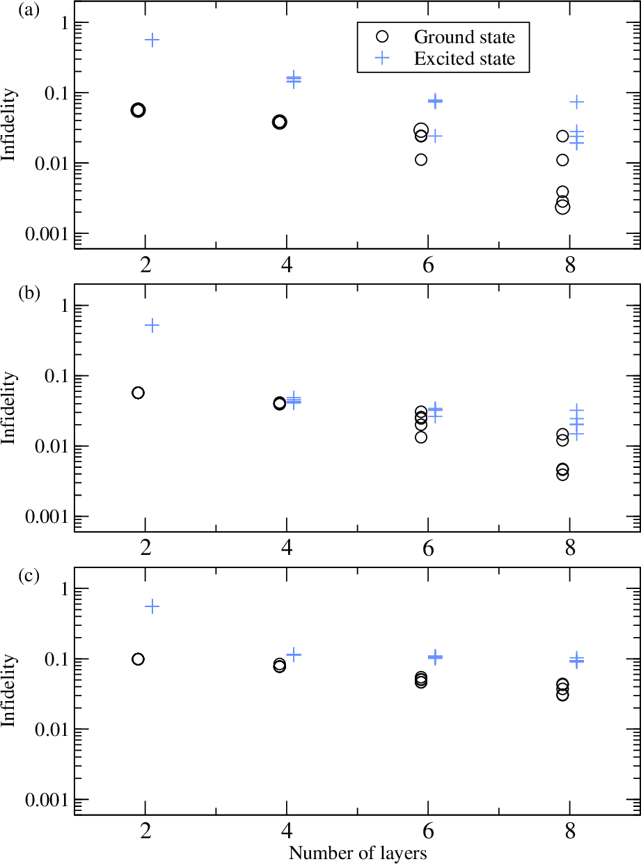
Figure 8 shows the calculated infidelity \(1 - |\langle \Psi_{\textrm{DMRG}}|\tilde{\Psi}\rangle|^{2}\) of the ground state and the first excited state for the three cases as a function of the number of layers \(L\). In each case five different random initial states are used. In all cases the infidelity is below \(\approx 0.05\) for the ground state and \(\approx 0.1\) for the excited state with \(L \geq 6\). We therefore use the \(L=6\) results with the lowest infidelity in our hardware demonstration.
Each two-qubit unitary \(U_{l b}\) is converted into quantum gates with up to three two-qubit gates. We apply qiskit.synthesis.two_qubit_decompose function in Qiskit, which internally uses the KAK
decomposition [44]. For the ground state (the excited state), the quantum circuits transpiled by Qiskit contain 98, 153, and 227
(110, 174, and 227) two-qubit basis gates (cz gates) for 16, 24, and 32 qubits, respectively.
4.2 Error mitigation↩︎
| (10e,8o) | (10e,12o) | (10e,16o) | ||
|---|---|---|---|---|
| No mitigation | Ground state | \(0.742 \pm 0.005\) | \(0.615 \pm 0.003\) | \(0.540 \pm 0.007\) |
| Excited state | \(0.756 \pm 0.005\) | \(0.562 \pm 0.015\) | \(0.526 \pm 0.007\) | |
| ZNE (gate-folding) | Ground state | \(0.940 \pm 0.007\) | \(0.889 \pm 0.011\) | \(0.849 \pm 0.014\) |
| Excited state | \(0.941 \pm 0.004\) | \(0.892 \pm 0.010\) | \(0.824 \pm 0.013\) | |
| QESEM | Ground state | \(0.996 \pm 0.011\) | \(0.969 \pm 0.015\) | \(0.968 \pm 0.010\) |
| Excited state | \(1.008 \pm 0.013\) | \(0.985 \pm 0.017\) | \(0.985 \pm 0.013\) | |
| Exact | Ground state | \(0.998\) | \(0.997\) | \(0.999\) |
| Excited state | \(1.000\) | \(0.996\) | \(0.994\) |
We apply two error mitigation techniques: (i) gate-folding based zero noise extrapolation (ZNE) implemented in Qiskit and (ii) quasi-probabilistic error mitigation approach implemented in QESEM [22] available via Qiskit Function [45].
The gate-folding based ZNE amplifies noise by replacing specific gates (two-qubit gates) with equivalent but redundant gate sequences (e.g. \(U \to U U^{\dagger} U\)). The obtained noisy results are extrapolated to get
noise-free expectation value results. The extrapolated results are not guaranteed to be unbiased. We set Qiskit option resilience_level=2 [46], which uses ZNE noise factors \((1, 3, 5)\). This option also activates readout error mitigation and measurement twirling via the model-free technique called twirled readout error
extinction (TREX) [47].
Unlike ZNE, the quasi-probability error mitigation method underlying QESEM is an unbiased method. QESEM extends the applicability of probabilistic error cancellation (PEC) [19], [48] by incorporating techniques such as the active-volume identification and multi-type quasi-probability decompositions which allows mitigation of non-Clifford two-qubit gates [22]. QESEM first performs device characterization, and this information is used for error suppression, noise-aware transpilation, error model construction, and building quasi-probability decomposition for implementing the inverse noise channels. The mitigated results and their variances are obtained by processing the measurement data of mitigation circuits sampled from the ensemble defined by the quasi-probability decomposition. More details of this approach are described in Ref. [22].
For each setup, we carry out five independent sets of measurements with a target precision of 0.02. The corresponding number of shots per circuit in ZNE is about 2500. In QESEM, the number of total shots for each measurement set, including calibration, noise characterization, and mitigation, with 32 qubits varies from \(1.4 \times 10^6\) to \(2.1 \times 10^6\). The corresponding QPU time for each measurement set ranges approximately from 400 to 600 seconds.
4.3 Hardware results↩︎
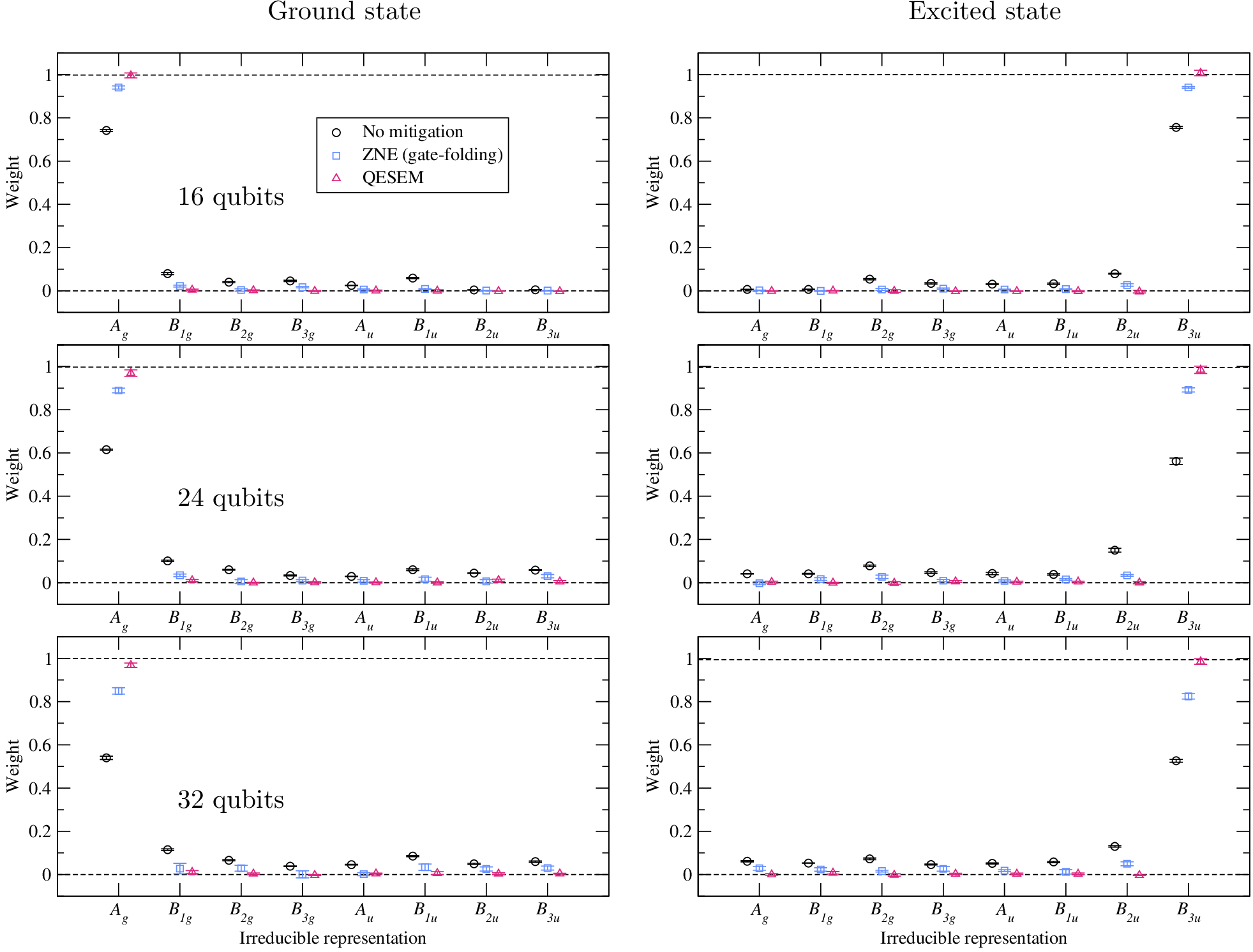
Figure 9 shows the hardware results executed on ibm_kawasaki for the ground state and the first excited state. The correct irreducible representations are \(A_{g}\) and
\(B_{3u}\) for the ground state and the excited state, respectively. The estimated weights of these irreducible representations are summarized in Table 6. Note that the exact results
in Table 6 deviate slightly from unity due to the approximate encoding.
Without error mitigation, the weights of the correct representations decrease as the number of qubits increases. In the 32-qubit results, the weights reduce to 0.540 for the ground state and 0.526 for the excited state. To further assess the quality of raw measurement results, independent measurements are performed which count the number of bitstrings with correct electron numbers, using \(10^{5}\) shots each. The probabilities of obtaining correct bitstrings for the ground state are 0.70, 0.55, and 0.36 for 16, 24, and 32 qubits, respectively. The corresponding values for the excited state are 0.68, 0.46, and 0.35, respectively. These poor results clearly show the importance of error mitigation.
The gate-folding based ZNE improves the quality of the results, but the results are biased. The results with QESEM’s quasi-probabilistic approach show the best agreement, with a maximum discrepancy of only a few percent. This comparison highlights the importance of accurate noise characterization and removal, and also validates the efficacy of our proposed method. This demonstration also suggests that our method can also be used for benchmarking quantum devices and error mitigation techniques, as our method requires no ancilla qubit and no or very little overhead for symmetry-adapted orbitals.
Although the present demonstration is based on the Pauli-based evaluation, which works only for abelian groups, our proposed method can also be applied to non-abelian symmetry groups with arbitrary basis functions. The hardware application of our method to a non-abelian case is an interesting direction for future research.
5 Conclusion↩︎
In this work, we presented a practical framework for studying point-group symmetry properties of many-electron wavefunctions on a quantum computer. We proposed an ancilla-free, basis-agnostic method to evaluate the weights of irreducible representations in a given wavefunction, which works for both abelian and non-abelian groups. Our numerical simulations on single Slater determinants and correlated wavefunctions show the usefulness of our method in preparing a trial state with a specific symmetry, as well as in assessing the quality of a wavefunction.
We also presented a hardware demonstration of our proposed method using up to 32 qubits of IBM’s superconducting quantum device ibm_kawasaki. By combining a tensor-network based state preparation scheme and advanced error mitigation
techniques, we successfully reproduced the correct weights of the irreducible representations for the ground state and the excited state of benzene.
We expect our methodology is useful for analyzing many-electron states prepared with more advanced quantum algorithms, and it also serves as a tool for benchmarking quantum devices and error mitigation techniques. The extension of the proposed method to other symmetry groups is also an interesting topic for future study.
R.S. thanks Ori Alberton, Asaf Berkovitch, Netanel Lindner, and Asif Sinay for technical advice on the use of QESEM. Molecular structures were visualized using VESTA [49].
6 Derivation of \(\sum_{\Gamma} w_{\Gamma} = 1\)↩︎
Here we show \(\sum_{\Gamma} w_{\Gamma} = 1\) is satisfied for \(w_{\Gamma}\) given in Eq. (3 ). The derivation is based on the orthogonality relationships of \(\chi_{\Gamma}(C)\) [4] \[\begin{align} \frac{1}{|G|}\sum_{C} r_{C} \chi^{*}_{\Gamma}(C) \chi_{\Gamma'}(C) &=& \delta_{\Gamma \Gamma'} \tag{20}\\ \frac{1}{|G|}\sum_{\Gamma} \chi^{*}_{\Gamma}(C) \chi_{\Gamma}(C') &=& \frac{1}{r_{C}} \delta_{C C'} \tag{21} \end{align}\] where \[r_{C} = \sum_{g \in C} 1 \label{eq:r95c}\tag{22}\] is the number of elements in \(C\). Noting that \[d_{\Gamma} = \chi_{\Gamma}(E)\] with \(E\) the identity operation, from Eq. (3 ) \[\begin{align} \sum_{\Gamma} w_{\Gamma} &=& \sum_{C}\frac{1}{|G|} \sum_{\Gamma} \chi_{\Gamma}^{*}(C) \chi_{\Gamma}(E) \sum_{g \in C} \langle \Psi |\hat{g}|\Psi\rangle \nonumber\\ &=& \sum_{C} \frac{\delta_{C E}}{r_{E}} \sum_{g \in C} \langle \Psi |\hat{g}|\Psi\rangle \nonumber\\ &=& \langle \Psi |\hat{E}|\Psi\rangle =1. \label{eq:sum95w95gamma} \end{align}\tag{23}\] Here \(r_{E} = 1\) is used. Equation (23 ) shows that \(\sum_{\Gamma} w_{\Gamma} = 1\) is satisfied independently of \(\langle \Psi | \hat{g}|\Psi \rangle\) for \(g \neq E\).