Proof. The strategyproofness of 1 follows from the strategyproofness of \(\cwmed\) ([prop:cwmed-properties]), since the agents have no control over the random rotation matrix the algorithm chooses.

Computing 1 can be done in \(O(d^3 + nd^2)\) as the rotation matrix may be sampled in \(O(d^3)\) (see [69], [70]), the matrix-vector multiplication takes \(O(n d^2)\) and median selection takes \(O(nd)\) time (\(O(n)\) time for median computation in each of the \(d\) coordinates). ◻

Proof. Sampling a random matrix \(R \in SO(2)\) is equivalent to sampling a random \(2 \times 2\) matrix \(R_\theta\) where \(\theta \sim U\crl*{[0,2\pi)}\) [34]. Also, \(\rcwmed\) is \(\frac{\pi}{2}\)-periodic, as any \(\frac{\pi}{2}\) rotation does not change the location of the \(\cwmed\): while the names of the axes may change, the axes lines remain the same. Thus, the median in each axis remains the same as well. ◻

Proof. It follows from the \(\ell_1\) norm definition that \(\norm{R_\theta v}_1 = \abs{(R_\theta v)_1} + \abs{(R_\theta v)_2}\), and thus we get the desired by showing: \[\E\brk*{\abs{(R_\theta v)_1} + \abs{(R_\theta v)_2}} = \frac{4}{\pi} \norm{v}_2.\]

Let \((y,\alpha)\) be the polar representation of \(v\). Then: \[(R_\theta v)_1 = y (cos(\theta) cos(\alpha) - sin(\theta) sin(\alpha)) = y \;cos(\theta+\alpha),\] \[(R_\theta v)_2 = y (sin(\theta) cos(\alpha) + cos(\theta) sin(\alpha)) = y \;sin(\theta+\alpha).\] Thus: \[\begin{align} \E\brk*{\abs{(R_\theta v)_1} + \abs{(R_\theta v)_2}} &= \int_{0}^{\frac{\pi}{2}} \frac{2}{\pi} y \prn*{ \abs{cos(\theta+\alpha)} + \abs{sin(\theta+\alpha)}} d\theta \\ & = \frac{2 y}{\pi} \int_{\alpha}^{\alpha + \frac{\pi}{2}} \prn*{\abs{cos(u)} + \abs{sin(u)}} du \\ & \stackrel{(\star)}{=} \frac{2 y}{\pi} \int_{0}^{\frac{\pi}{2}} \prn*{\abs{cos(u)} + \abs{sin(u)}} du = \frac{2 y}{\pi} \prn*{1 + 1} = \frac{4}{\pi} \;\norm{v}_2, \end{align}\] where equality \((\star)\) holds as \(f(u) = |cos(u)| + |sin(u)|\) is \(\frac{\pi}{2}\)-periodic: \[f\prn*{u + \frac{\pi}{2}} = \abs*{cos\prn*{u + \frac{\pi}{2}}} + \abs*{sin\prn*{u + \frac{\pi}{2}}} = \abs{- sin(u)} + \abs{cos(u)} = f(u).\] ◻

Proof. Let \(g = \geomed(P)\) and let \(h\) be the location returned by the algorithm. For any \(i \in [n]\): let \(v_i = p_i - g\). Let \(OPT = \sum_{i \in [n]} \norm{p_i - g}_q = \sum_{i \in [n]} \norm{v_i}_q\).

For any vector \(v \in \R^2\) let \(v_1\), \(v_2\) denote the \(x\), \(y\) coordinates of \(v\), respectively.

For any \(j \in [2]\): let \((h')_j = median(\crl*{(R p_i)_j})\) be the median of the multiset of \(j\) coordinates of \(P'\) (for \(j=1\) it is the \(x\) axis and for \(j=2\) it is the \(y\) axis obtained after a rotating by \(\theta\)).

\(ALG_\theta\), the cost of the algorithm given \(\theta\) is: \[\begin{align} ALG_{\theta} & = \sum_{i \in [n]} \norm{p_i - h}_q \le \sum_{i \in [n]} \norm{p_i - h}_2 = \sum_{i \in [n]} \norm{R_\theta p_i - R_\theta h}_2 \\ & \le \sum_{i \in [n]} \norm{R_\theta p_i - h'}_1 \le \sum_{i \in [n]} \norm{R_\theta p_i - R_\theta g}_1 = \sum_{i \in [n]} \norm{R_\theta v_i}_1, \numberthis \label{eq:alg-bound-each-comp-by-theta} \end{align}\tag{1}\] where the first inequality holds as \(q \ge 2\) , the second equality is due to the fact that rotation is an isometry for \(\norm{\cdot}_2\), the second inequality is due to the fact that \(\norm{x}_2 \le \norm{x}_1\) for any \(x \in \R^2\), and the last inequality is due to the fact that \(h'_j\) is the minimizer of function \(f_j(x) = \sum_{i \in [n]} \abs{a^{(j)}_i - x}\) (as \(h'_j\) is the median of the projected points).

By taking the expectation (on 1 ) and applying [lem:expected-abs-value-of-each-rotated-component] we get that the expected cost of the algorithm is: \[\E_\theta[ALG_\theta] \le \sum_{i \in [n]} \frac{4}{\pi} \norm{v_i}_2 \stackrel{\text{since } q \ge 2}{\le} \;\sum_{i \in [n]} \frac{4}{\pi} \prn*{2^{\nf{1}{2} - \nf{1}{q}}} \norm{v_i}_q = \frac{4}{\pi} \prn*{2^{\nf{1}{2} - \nf{1}{q}}} OPT.\] ◻

Proof. Consider the instance \(P \subset \R^2\): \(k\) points in \((1,0)\), \(k\) points in \((0,1)\) and \(1\) point in \((-M,-M)\), for \(M\gg1 \in \N\) and \(k = M^2\).

Let \(A = (1,0)\), \(B = (0,1)\) and \(C = (-M, -M)\). Consider the new point locations \(P'\) obtained by a rotation by \(\theta \in [0,\frac{\pi}{2}]\). Let \(s = sin(\theta)\) and \(c = cos(\theta)\). Then the new locations of the points are \(A', B', C'\) where: \(A' = R_\theta \cdot A = (c,s)\), \(B' = R_\theta \cdot B = (-s,c)\) and \(C' = R_\theta \cdot C = (-M(c-s), -M(c+s))\).

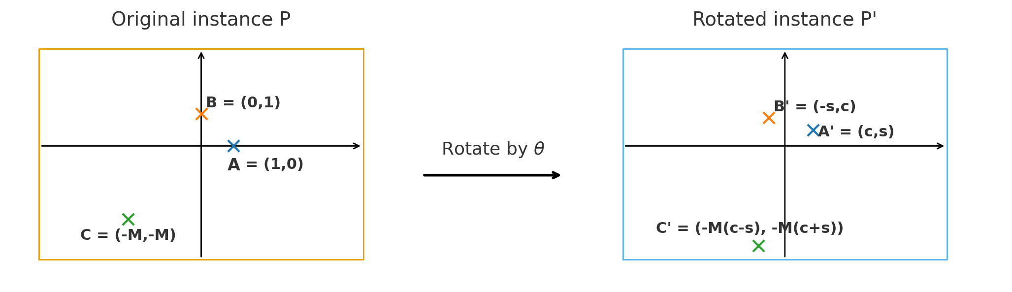
Let \(m_\theta = (x_\theta, y_\theta)\) denote the coordinate-wise median of the multi-set of rotated points \(P'\). Since rotation is an isometry, the social cost of \(m_\theta\) w.r.t. \(P'\) is the same as the social cost of \(m_\theta\) rotated back by \(-\theta\) w.r.t. the original multi-set of points \(P\).

Since there are \(2k+1\) points, the median in each coordinate is the \(k+1\)-st order statistic.

• For \(\theta \in [0,\frac{\pi}{4})\): \(c \ge s\). If \(C'_1 \le -s\) then \(x_\theta = B'_1 = -s\), and otherwise \(x_\theta = C'_1 = -M(c-s)\).

  For the \(y\) axis: \(y_\theta = s\) always, as the median is \(A'_2\).

• For \(\theta \in [\frac{\pi}{4}, \frac{\pi}{2})\): \(c \le s\). if \(C'_1 \ge c\) then \(x_\theta = A'_1 = c\), and otherwise \(x_\theta = C'_1 = -M(c-s)\).

  For the \(y\) axis: \(y_\theta = c\) always, as the median is \(B'_2\).

Let \(W_M := \crl*{\theta \in [0,\frac{\pi}{2}) \mid C'_1 \in (-s, c)}\) be the set of angles for which \(x_\theta = C'_1\). We show that for most angles (all but a \(O(\frac{1}{M})\) fraction) it must be that \(x_\theta \neq C'_1\):

We are now ready to lower bound the expected cost of the algorithm.

The optimal solution cost is at most the cost of the solution of placing the facility at \(A = (1,0)\): \(OPT \le \sqrt{2}k + O(M) = \sqrt{2}k + O(\sqrt{k})\) .

Thus, from [clm:expected-cost-of-alg-at-most-4-pi-sqrt-2-times-k]: \[\frac{\E[ALG]}{OPT} \ge \frac{\frac{4}{\pi} \;k \sqrt{2} - O(\sqrt{k})}{\sqrt{2} k + O(\sqrt{k})} \stackrel{k \to \infty}{\to} \frac{4}{\pi}.\] ◻

Proof sketch of [thm:rrcwmed-expected-approximation-ratio-Rd]. For the upper bound, an approach similar to the one we’ve taken in [lem:R2-ub] for \(\R^2\) may lead to a slightly better \(1.5\) bound for \(\R^3\), but it does not scale well; it leads to a ratio of \(\Omega(\sqrt{d})\) for large \(d\) values (e.g. see the \(\Omega(\sqrt{d})\) analysis for the projection median approximation of [72]). The \(\sqrt{6 \sqrt{3} - 8}\) upper bound follows directly from the approximation ratio upper bound of \(\cwmed\) (see [prop:cwmed-properties]): [1] show that the approximation ratio of \(\cwmed\) is bounded by \(\sqrt{6 \sqrt{3} - 8}\) by analyzing a factor revealing optimization problem. Since \(\rrcwmed\) is \(\cwmed\) with random rotations, its expected cost is upper bounded by the worst-case cost of \(\cwmed\).

We now show that a construction analysis which closes most of the remaining gap. While the idea in the construction is very similar to our two dimensional one (two clusters and an outlier construction), the analysis requires “heavier machinery” — we use random matrix theory and high-dimensional probability to show that the expected distance of each cluster point from the random returned point is large.

Let \(d \gg 1\) and let \(k = \floor{\sqrt{d}}\), \(M = \sqrt{k}\). The instance \(P\) we observe contains: \(k\) copies of \(e_1\), \(k\) copies of \(e_2\) and a single copy of \(-M(e_1 + e_2)\). Our goal is to show that \(\E[ALG] \approx 2k\), which implies that the approximation ratio is roughly \(\sqrt{2}\) (as \(OPT \le k\sqrt{2} + O(\sqrt{k})\)).

Let \(R \in SO(d)\) be the uniformly sampled rotation matrix, let \(a = R e_1\), \(b = R e_2\) and \(c = R (-M(e_1+e_2)) = -M(a+b)\). Let \(m\) be the \(\cwmed\) of the rotated multi-set of points \(R P\). For any \(j \in [d]\), let \(m_j\) be the median for coordinate \(j\). In coordinate \(j\) the distinct locations of the rotated points are \(a_j, b_j, c_j\). Since \[\E[ALG] \ge k \prn*{\E\brk*{\norm{a - m}_2} + \E\brk*{\norm{b - m}_2}}, \numberthis \label{eq:alg-expected-val-sqrt2-lb-of-randcwmed-sketch}\tag{5}\] we will show that \(\E\brk*{\norm{a - m}_2}\) and \(\E\brk*{\norm{b-m}_2}\) are approximately \(1\), which implies the desired.

For each coordinate \(j\in[d]\), define the event \(D_j\) that the outlier coordinate \(c_j\) lies between \(a_j\) and \(b_j\) (i.e., \(\min\{a_j,b_j\}\le c_j\le \max\{a_j,b_j\}\)). On coordinates where \(D_j\) fails, the outlier does not affect the median: \(m_j\in\{a_j,b_j\}\). Using an explicit case analysis (formalized as a claim in the full proof), we obtain the inequality \[\label{eq:abm-quad-sketch} \|a-m\|_2^2+\|b-m\|_2^2 \;\ge\; \|a-b\|_2^2 -\sum_{j=1}^d \frac{(a_j-b_j)^2}{2}\,\mathbf{1}\{D_j\}.\tag{6}\] Since \(a\) and \(b\) are orthonormal columns of \(R\), we have \(\|a-b\|_2^2=\|a\|_2^2+\|b\|_2^2-2\langle a,b\rangle=2\). Taking expectations in 6 and using symmetry (that is, \(\E\brk*{\norm{a-m}_2^2} = \E\brk*{\norm{b-m}_2^2}\)) yields \[\label{eq:Ez2-core-sketch} \mathbb{E}\|a-m\|_2^2 \;\ge\; 1-\frac{1}{4}\sum_{j=1}^d \mathbb{E}\bigl[(a_j-b_j)^2\,\mathbf{1}\{D_j\}\bigr].\tag{7}\] Thus, the key task is to show that the total “bad-event mass” on the RHS is \(O(1/k)\). Define normalized coordinates \(U_j:=\sqrt{\frac{d}{2}}(a_j+b_j),\; V_j:=\sqrt{\frac{d}{2}}(a_j-b_j)\). Then \((a_j-b_j)^2=\frac{2}{d}V_j^2\), and it follows from \(c_j=-M(a_j+b_j)\) that \(D_j\) occurs iff \(|U_j|\le t\,|V_j|\) where \(t:=\frac{1}{2M+1}\).

We now use the Diaconis–Freedman normal approximation theorem for random orthogonal matrices (equivalently, the fact that finitely many coordinates of a Haar-uniform \(R\in SO(d)\) are close in total variation to i.i.d.Gaussians after the \(\sqrt d\) scaling) [33]. Concretely, for each fixed \(j\), the pair \((U_j,V_j)\) is \(O(1/d)\)-close in total variation to \((G_1,G_2)\) where \(G_1,G_2\stackrel{\text{i.i.d.}}{\sim}N(0,1)\). We show this implies \[\label{eq:tv-reduction} \mathbb{E}\!\left[V_j^2\,\mathbf{1}\{|U_j|\le t|V_j|\}\right] \;=\; \mathbb{E}\!\left[G_2^2\,\mathbf{1}\{|G_1|\le t|G_2|\}\right] + O(1/\sqrt{d}).\tag{8}\]

For \((G_1,G_2)\sim N(0,I_2)\), we show (by integral calculations) that \(\E\brk*{G_1^2 \indic{\abs{G_1} \le t \abs{G_2}}} \le O\prn*{\frac{1}{k}}\). Combining with 8 and the identity \((a_j-b_j)^2=\frac{2}{d}V_j^2\), we obtain \[\begin{align} \sum_{j=1}^d \mathbb{E}\bigl[(a_j-b_j)^2\,\mathbf{1}\{D_j\}\bigr] &= \sum_{j=1}^d \frac{2}{d}\,\mathbb{E}\!\left[V_j^2\,\mathbf{1}\{|U_j|\le t|V_j|\}\right]\nonumber\\ &\le 2\cdot O(1/M^3)\;+\;O(1/\sqrt{d})\nonumber\\ &= O(1/k), \label{eq:bad-mass-sketch} \end{align}\tag{9}\] using \(M=\sqrt{k}\) and \(d = \Theta( k^2)\).

Plugging 9 into 7 yields \[\label{eq:Ez2} \mathbb{E}\|a-m\|_2^2\;\ge\;1-O(1/k).\tag{10}\]

We wish to deduce⁸ that \(\E\brk*{\norm{a-m}_2} \ge 1 - O\prn*{\frac{1}{k}}\).

Let \(Z := \norm{a - m}_2\). We already have the second moment lower bound \(\E\brk*{Z^2} \ge 1 - O\prn*{\frac{1}{k}}\), and the goal is to show that \(\E\brk*{Z} \ge 1 - O\prn*{\frac{1}{k}}\). By the definition of the variance of \(Z\): \[\label{eq:sketch-var-Z} \prn*{\E[Z]}^2 = \E[Z^2] - Var(Z).\tag{11}\] The idea in the rest of the lemma is to show that \(Var(Z) = O\prn*{\frac{1}{k}}\) and thus by we’ll get the desired.

Consider the function \(f(R):=\|Re_1-\mathrm{CWM}(RP)\|_2\) on \(SO(d)\) (so \(f(R) = Z\)). We show (in the full proof) that \(f\) is \(L\)-Lipschitz w.r.t.the Frobenius metric, with \(L=O(M)\). Then, we apply a concentration inequality for Lipschitz functions of random variables on \(SO(d)\) and get that \[Var(Z) \le O \prn*{\norm{Z - \E \brk*{Z}}_{\psi_2}^2} \le O\prn*{\norm{f(R) - \E \brk*{f(R)}}_{\psi_2}} \le O\prn*{\frac{1}{k}}.\]

Using \(\mathbb{E}[Z]^2=\mathbb{E}[Z^2]-\Var(Z)\) together with 10 and 11 , we conclude \[\label{eq:EZ} \mathbb{E}\|a-m\|_2\;\ge\;1-O(1/k).\tag{12}\]

Combining 5 with 12 and symmetry, \[\E[ALG] \ge 2k\cdot (1-O(1/k)) = 2k-O(1).\] Since \(OPT \le \sqrt{2}k + O\prn*{\sqrt{k}}\) we get the desired: \[\frac{\E\brk{ALG}}{OPT} \ge \sqrt{2} - O\prn*{\frac{1}{k}} = \sqrt{2} - O\prn*{\frac{1}{\sqrt{d}}}.\] ◻

Proof. Strategyproof is immediate from the fact that the prediction is independent from the agent reports, and from the strategyproofness of \(\rrcwmed\). Let \(ALG_\theta\) denote the cost of \(\rrcmp\) given any sampled \(\theta\), and let \(OPT\) be the cost of the optimal solution.

The approximation ratio of \(\rrcmp\) is upper bounded by that of \(\cmp\). Specifically, for any instance \(I\) and any \(\theta \in [0, \frac{\pi}{4})\) sampled by \(\rrcmp\), the cost incurred by \(\rrcmp\) on instance \(I\) equals the cost incurred by \(\cmp\) on the rotated instance \(I_\theta\), obtained from \(I\) by rotating all points by \(\theta\). Consequently, \(\rrcmp\) directly inherits the approximation guarantees of \(\cmp\) established by [18]: \[\E[ALG_\theta] \le \min\crl*{\frac{\sqrt{2c^2 + 2}}{1+c} + \eta, \frac{\sqrt{2c^2+2}}{1-c}} OPT.\]

W.l.o.g., assume that \(\hat{g} = 0\). Otherwise, we may translate the instance by \(t = -\hat{g}\). The rotated translated instance is equivalent to the original rotated instance translated by \(R_{\theta} t\), where \(R_{\theta}\) denotes the rotation matrix. Consequently, the resulting \(\rcwmed\) is equal to the original one, translated by \(R_{\theta} t\). After rotating back by \(R_{-\theta}\), we obtain the same solution translated by \(t\). Therefore, all pairwise distances remain unchanged, and the transformed instance preserves the same approximation ratio.

Let \(g\) be the geometric median. Then \(OPT = \sum_{i=1}^n \norm{p_i - g}_2\). Let \(m = \floor{cn} \in \N\).

Let \(\hat{h}_\theta\) be the coordinate-wise median of the rotated dataset \(R_\theta(P \cup \hat{P})\), and let \(h'_\theta\) be the coordinate-wise median of the rotated dataset without the copies of the prediction: \(R_\theta P\). Let \(h\) be the location returned by \(\rrcmp\). We start in a similar way to the proof of [lem:R2-ub]: \[\begin{align} ALG_\theta & = \sum_{i\in[n]} \norm{p_i - h}_2 = \sum_{i\in[n]} \norm{R_\theta p_i - R_\theta h}_2 \le \sum_{i\in[n]} \norm{R_\theta p_i - \hat{h}_\theta}_1, \numberthis \label{eq:ALG-theta-tmp-bound-learning-aug} \end{align}\tag{13}\] where the second equality holds as \(\norm{\cdot}_2\) is invariant to rotation and the inequality is due to the fact that \(\norm{x}_2 \le \norm{x}_1\) for any \(x \in \R^2\).

First, we show the consistency improvement. By 13 :

\[\begin{align} ALG_\theta &\le \sum_{i\in[n]} \norm{R_\theta p_i - \hat{h}_\theta}_1 + m \norm{R_\theta \hat{g} - \hat{h}_\theta}_1 - m \norm{R_\theta \hat{g} -\hat{h}_\theta}_1 \\ & \le \sum_{i\in[n]} \norm{R_\theta p_i - R_\theta g}_1 + m \norm{R_\theta \hat{g} - R_\theta g}_1 - m \norm{R_\theta \hat{g} - \hat{h}_\theta}_1 \\ & = \sum_{i\in[n]} \norm{R_\theta p_i - R_\theta g}_1 + m \prn*{\norm{R_\theta g}_1 - \norm{\hat{h}_\theta}_1}, \numberthis \label{eq:alg-theta-rr-cmp-tmp} \end{align}\tag{14}\]

where the inequality is due to the fact that \(\hat{h}_\theta\) is the \(\scost_1\) minimizer solution of \(R_\theta \prn*{P \cup \hat{P}}\), as its \(\cwmed\) (due to [prop:cwmed-properties]), and thus \(R_\theta \;g\) has a larger \(\scost_1\) cost. The last equality holds as \(\hat{g} = 0\).

From 14 and the fact that \(m = \floor{cn}\): \[\label{eq:rrcmp-expected-ub-tmp} \E[ALG_\theta] \le \E\brk*{\sum_{i\in[n]} \norm{R_\theta p_i - R_\theta g}_1} + cn \E\brk*{\norm{R_\theta g}_1 - \norm{\hat{h}_\theta}_1}.\tag{15}\]

\(\norm{R_\theta g}_1 - \norm{\hat{h}_\theta}_1 \le \norm{R_\theta g}_1 = \norm{R_\theta g - R_\theta \hat{g}}_1\), and thus, by plugging [lem:expected-abs-value-of-each-rotated-component] in 15 : \[\begin{align} \E[ALG_\theta] &\le \frac{4}{\pi} OPT + c n \frac{4}{\pi} \E \brk*{\norm{R_\theta g - R_\theta \hat{g}}_2} = \frac{4}{\pi} OPT + c n \frac{4}{\pi} \norm{g - \hat{g}}_2 \\ & = \frac{4}{\pi} \prn*{1 + c \eta} OPT, \end{align}\] where the one before last equality holds by the fact rotation is an isometry, and the last equality is due to the definition of \(\eta\).

For the robustness upper bound, by 13 and [lem:geometric-median-approx-robustness]: \[\begin{align} ALG_\theta & \le \sum_{i\in[n]} \norm{R_\theta p_i - \hat{h}_\theta}_1 = \scost_1(R_\theta P, \hat{h}_\theta) \le \prn*{1 + \frac{2c}{1-c}}\scost_1(R_\theta P, h'_\theta) \\ & \le \prn*{1 + \frac{2c}{1-c}}\scost_1(R_\theta P, R_\theta g) = \prn*{1 + \frac{2c}{1-c}} \sum_{p \in P} \norm{R_\theta (p - g)}_1, \end{align}\] where the last inequality is due to the fact that \(h'_\theta\) is the \(\scost_1\) minimizer solution of dataset \(R_\theta P\). By taking expectation and using [lem:expected-abs-value-of-each-rotated-component] we get: \[\E\brk*{ALG_\theta} \le \prn*{1 + \frac{2c}{1-c}} \E\brk*{\sum_{p \in P} \norm{R_\theta (p - g)}_1} = \prn*{1 + \frac{2c}{1-c}} \frac{4}{\pi} \sum_{p \in P} \norm{p - g}_2 = \frac{4}{\pi} \frac{1+c}{1-c} OPT.\] ◻

Proof. Let \(n \gg 1\). Consider the instance \(P = \crl*{p_0, \ldots ,p_{n-1}}\) where \(p_k = \prn*{cos(\frac{2\pi k}{n}), sin(\frac{2\pi k}{n})}\) for \(k \in \crl*{0,\ldots,n-1}\). The point \(y=0\) has cost \(\scost(P,y) = \sum_{i=0}^{n-1} 1 = n\) and thus the optimal solution has cost at most \(n\): \(OPT \le n\). Let \(A\) be a GRD mechanism, and let \(ALG\) be its cost. We show that for any dictator choice \(p_k \in P\) of \(A\), the social cost of this solution is approximately \(\frac{4}{\pi} n\).

Assume w.l.o.g. that \(p_k = p_0\) (due to symmetry the cost is the same). The distance between \(p_0\) and \(p_j\) separated by the angle \(\frac{2\pi j}{n}\) is the chord length: \[\norm{p_0 - p_j}_2 = 2 sin\prn*{\frac{\pi j}{n}}.\]

Therefore \(ALG = 2 \sum_{j=1}^{n-1} sin\prn*{\frac{\pi j}{n}} =2 \;cot(\frac{\pi}{2n})\) where the last equality follows from the identity:

The proof of [clm:trigo-identity] follows from standard trigonometric identities and the sum of a telescoping series, and we provide it in 10.

By the Taylor expansion of \(cot\), the cost of \(A\) is: \[ALG = 2 \;cot(\frac{\pi}{2 n}) = 2 \prn*{\frac{2n }{\pi} - O\prn*{\frac{1}{n}}} = \frac{4n}{\pi} - O\prn*{\frac{1}{n}}.\]

Since the above holds for any \(p_k\), the above equation yields the desired by taking \(n \to \infty\). ◻

Proof. The idea is similar to the one of [thm:lb-rand-dict-R2], but we use the probabilistic method [35] rather than exhibiting an explicit worst-case instance: instead of choosing evenly spaced points, we sample i.i.d.points from the unit sphere. We will lower bound the algorithm’s cost with high probability and upper bound the optimum deterministically; by the probabilistic method there exists a fixed multi-set achieving the same bounds.

Let \(n \gg 1\). Let us observe the instance of points \(P = \crl*{Y_1, \ldots,Y_{n+1}} \subset \R^d\) where \(Y_1, \ldots,Y_{n+1}\) are i.i.d.random variables such that for each \(i \in [n+1]\): \(Y_i \sim U\crl*{S^{d-1}}\) is chosen randomly from the unit sphere. Let \(A\) be a GRD mechanism with cost \(ALG\).

Fix \(j \in [n+1]\). Without loss of generality assume \(Y_j = e_1 = (1,0,\ldots,0) \in \R^d\): indeed, condition on \(Y_j\) and apply an orthogonal map \(Q\) with \(QY_j=e_1\); the joint law of \(\crl*{QY_i}_{i\ne j}\) is the same as that of \(\crl*{Y_i}_{i\ne j}\) and all pairwise distances are preserved. Consider \(ALG_j\), the sum of distances of the points of \(P\) from point \(Y_j = e_1\). This is the cost of mechanism \(A\) in case it returns point \(Y_j\). Then \[\E[ALG_j] = \E_P [ALG_j] = \E_P \brk*{\sum_{Y_i \in P} \norm{Y_i - e_1}_2} = n \;\E_{X \sim U\prn*{S^{d-1}}}\brk*{\norm{X - e_1}_2}. \numberthis \label{eq:expected-sum-of-distances-from-e1}\tag{16}\]

The following lemma bounds \(\E\brk*{\norm{X-e_1}_2}\) as a function of the even moments of \(X_1\) where \(X = (X_1,\ldots,X_d) \sim U\prn*{S^{d-1}}\):

We defer the proof of [lem:random-sphere-vector-distance-from-e1] to 10.2.

The next lemma states a known fact about the even moments of \(X_1\) (see the proof of Proposition 2.5 in [34]):

Plugging [lem:even-moments-sphere] into [lem:random-sphere-vector-distance-from-e1] gives: \[\mathbb{E}\,\norm{X-e_1}_2 =\sqrt{2}\left( 1-\frac{1}{8d} -\frac{15}{128\,d(d+2)} -\frac{315}{1024\,d(d+2)(d+4)}-\cdots \right).\] In particular, \[\E \brk*{\norm{X-e_1}_2} = \sqrt{2}\prn*{1-\frac{1}{8d}}+O\!\prn*{\frac{1}{d^2}}.\]

Denote \(\mu_d := \E \brk*{\norm{X-e_1}_2} = \sqrt{2}\prn*{1-\frac{1}{8d}}+O\!\prn*{\frac{1}{d^2}}\). By 16 we have \[\E[ALG_j] \;=\; n\,\mu_d.\]

\(ALG_j\) is a sum of independent random variables that lie in \([0,2]\). By Hoeffding’s inequality [73], for any \(t>0\), \[\Pr\prn*{ALG_j \le n\mu_d - t} \;\le\; \exp\prn*{-\frac{t^2}{2n}}.\] By a union bound over \(j\in[n+1]\), \[\Pr\prn*{\min_{j\in[n+1]} ALG_j \le n\mu_d - t} \;\le\; (n+1)\,\exp\prn*{-\frac{t^2}{2n}}.\] Taking \(t=\sqrt{2n}\log\prn*{n+1}\) gives, with probability at least \(1-\tfrac{1}{n+1}\), \[\min_{j\in[n+1]} ALG_j \;\ge\; n\mu_d - t.\]

Since a GRD mechanism returns one of the points \(Y_j\), \(\E_R\brk*{ALG}\) (expectation over the internal randomness \(R\) of \(A\)) is a convex combination of the \(ALG_j\), and hence \[\E_R\brk*{ALG} \;\ge\; \min_{j\in[n+1]} ALG_j.\] Therefore, w.p. at least \(1-\tfrac{1}{n+1}\) over the draw of \(P\), \(\E_R\brk*{ALG} \ge n\mu_d - \sqrt{2n}\log\prn*{n+1}\). By the probabilistic method, there exists a deterministic multi-set \(P\) for which the above inequality holds.

On the other hand, in any such instance \(\mathrm{OPT} \le \abs{P}=n+1\) (placing the facility at the origin yields cost \(n+1\)). Hence for that \(P\), \[\frac{\E_R\brk*{ALG}}{\mathrm{OPT}} \ge \frac{n\mu_d - \sqrt{2n}\log\prn*{n+1}}{n+1} = \mu_d \frac{n}{n+1} - O \prn*{\tfrac{\log n}{\sqrt{n}}}.\] Letting \(n\to\infty\) (with \(d\) fixed) and recalling \(\mu_d=\sqrt{2}\prn*{1-\frac{1}{8d}}+O \prn*{\frac{1}{d^2}}\) proves \[\frac{\E_R\brk*{ALG}}{\mathrm{OPT}} \;\ge\; \sqrt{2}\prn*{1 - O\prn*{\frac{1}{d}}}.\] This completes the proof. ◻

Proof. For the upper bound, an approach similar to the one we’ve taken in [lem:R2-ub] for \(\R^2\) may lead to a slightly better \(1.5\) bound for \(\R^3\), but it does not scale well: it leads to a ratio of \(\Omega(\sqrt{d})\) for large \(d\) values (e.g. see the \(\Omega(\sqrt{d})\) analysis for the projection median approximation of [72]).

The \(\sqrt{6 \sqrt{3} - 8}\) upper bound follows directly from the approximation ratio upper bound of \(\cwmed\) (see [prop:cwmed-properties]): [1] show that the approximation ratio of \(\cwmed\) is bounded by \(\sqrt{6 \sqrt{3} - 8}\) by analyzing a factor revealing optimization problem. Since \(\rrcwmed\) is \(\cwmed\) with random rotations, its expected cost is upper bounded by the worst-case cost of \(\cwmed\).

We now show that a construction analysis which closes most of the remaining gap. While the idea in the construction is very similar to our two dimensional one (two clusters and an outlier construction), the analysis requires “heavier machinery” — we use a result of [33] in random matrix theory which shows that most of the coordinates of the rotated points roughly (up to small total variation distance) follow standard i.i.d. Gaussian distributions for large \(d\) values. We use this to get a lower bound on the expected squared distance of a cluster point from the resulting median. Then we use concentration of measure results in high-dimensional probability to show that the variance of the distance is low, to deduce that the expected distance is low as well.

Let \(d \gg 1\) and let \(k = \floor{\sqrt{d}}\), \(M = \sqrt{k}\). The instance \(P\) we observe contains: \(k\) copies of \(e_1\), \(k\) copies of \(e_2\) and a single copy of \(-M(e_1 + e_2)\).

Like before, \(OPT\) is upper bounded by \(\sqrt{2} k + O(\sqrt{k})\). Our goal is now to show that \(\E[ALG] \approx 2k\), which implies that the approximation ratio is roughly \(\sqrt{2}\).

Let \(R \in SO(d)\) be the uniformly sampled rotation matrix, let \(a = R e_1\), \(b = R e_2\) and \(c = R (-M(e_1+e_2)) = -M(a+b)\). Let \(m\) be the \(\cwmed\) of the rotated multi-set of points \(R P\). For any \(j \in [d]\): Let \(m_j\) be the median in coordinate \(j\). In coordinate \(j\) the distinct locations of the rotated points are \(a_j, b_j, c_j\).

Since \[\E[ALG] \ge k \prn*{\E\brk*{\norm{a - m}_2} + \E\brk*{\norm{b - m}_2}}, \numberthis \label{eq:alg-expected-val-sqrt2-lb-of-randcwmed}\tag{17}\] we will show that \(\E\brk*{\norm{a - m}_2}\) and \(\E\brk*{\norm{b-m}_2}\) are approximately \(1\), which implies the desired (as \(OPT = k\sqrt{2} + O(\sqrt{k})\)).

\(\E\brk*{\norm{a-m}_2} = \E\brk*{\norm{b-m}_2}\) due to symmetry, and thus it is enough to show that \(\E\brk*{\norm{a-m}_2} \approx 1\). More accurately, we show that \(\E\brk*{\norm{a-m}_2} \ge 1 - O\prn*{\frac{1}{\sqrt{k}}}\).

Let \(D_j\) denote the “bad” (rare) event where \(c_j\) lies between \(a_j\) and \(b_j\).

We first give the two following technical claims:

The proofs of [clm:Dj-equiv-condition] and [clm:tech-clm-event-Dj] are quite straightforward, and we defer them to 8.2, 8.3.

We use [clm:tech-clm-event-Dj] and get: \[\begin{align} \norm{a-m}_2^2 + \norm{b-m}_2^2 & = \sum_{j=1}^d \prn*{a_j - m_j}^2 + \prn*{b_j - m_j}^2 \\ & =\sum_{j \in [d]} (a_j - b_j)^2 \\ & \;\;\;\;+ 2 \sum_{j \in [d]} \prn*{\prn*{m_j - \frac{a_j + b_j}{2}}^2 - \frac{\prn*{a_j-b_j}^2}{4}} \indic{D_j} \\ & \ge 2 - \sum_{j \in [d]} \prn*{ \frac{\prn*{a_j-b_j}^2}{2}} \indic{D_j}, \end{align}\]

where the inequality is due to the fact that \(\prn*{m_j - \frac{a_j + b_j}{2}}^2 \ge 0\) and the fact that \(\norm{a-b}_2^2 = \norm{a}_2^2 - 2 \langle a,b\rangle + \norm{b}_2^2 = 2\) as \(\norm{a}_2 = \norm{b}_2 = 1\) and \(a,b\) are orthogonal.

Since \(\E\brk*{\norm{a-m}_2^2} = \E\brk*{\norm{b-m}_2^2}\) (due to symmetry), the above inequality yields: \[\label{eq:bound-norm-of-a-minus-m} \E\brk*{\norm{a-m}_2^2} \ge 1 - \frac{1}{2} \E \brk*{\sum_{j \in [d]} (a_j - b_j)^2 \indic{D_j}} = 1 - \frac{1}{2} \sum_{j \in [d]} \E\brk*{(a_j - b_j)^2 \indic{D_j}}.\tag{18}\]

In the next lemma, we show that the last term in 18 is negligible:

By [lem:negligible-a95j-minus-b95j], and 18 we get that \[\label{eq:squared-norm-a-minus-m-lb} \E\brk*{\norm{a-m}_2^2} \ge 1 - O\prn*{\frac{1}{k}}.\tag{21}\] The following lemma shows that this implies that \(\E\brk*{\norm{a-m}_2} \ge 1 - O\prn*{\frac{1}{k}}\):

By [lem:norm-a-minus-m-lb] and 17 : \(\E[ALG] \ge 2k - O(1)\). Since \(OPT \le \sqrt{2}k + O(1)\) we get the desired: \[\frac{\E\brk{ALG}}{OPT} \ge \sqrt{2} - O\prn*{\frac{1}{k}} = \sqrt{2} - O\prn*{\frac{1}{\sqrt{d}}}.\] ◻

Proof. \(c_j \in [a_j, b_j]\) iff \((a_j - c_j)(b_j - c_j) \le 0\). By writing \(s := a_j + b_j\), \(d := a_j - b_j\), we get \(a = \frac{s+d}{2}, b = \frac{s-d}{2}\). Since \(c_j = -M s\): \[a_j - c_j = \frac{s+d}{2} + Ms = \frac{(2M + 1)s + d}{2}, \quad b_j - c_j = \frac{s-d}{2} + Ms = \frac{s(2M+1) - d}{2}.\] Thus \(c_j \in [a_j, b_j]\) iff \[\prn*{\frac{(2M + 1)s + d}{2}}\prn*{\frac{s(2M+1) - d}{2}} \le 0,\] or equivalently iff \((2M+1)\abs{s} \le \abs{d}\), which implies:

\[c_j \in [a_j, b_j] \iff \abs{a_j + b_j} \le \frac{\abs{a_j - b_j}}{2M + 1},\] ◻

Proof. We wish to show: \[\prn*{a_j - m_j}^2 + \prn*{b_j - m_j}^2 = (a_j - b_j)^2 + 2\prn*{\prn*{m_j - \frac{a_j + b_j}{2}}^2 - \frac{\prn*{a_j-b_j}^2}{4}} \indic{D_j}.\]

For the sake of abbreviation let \(x = a_j, z = b_j\) and \(y = c_j\), \(m = \frac{x+z}{2}\) and \(r = \frac{\abs{x-z}}{2}\). We now have two cases. In the first case, \(y \notin [x,z]\). In this case \(m_j \in \crl*{x,z}\) which implies that \((x-m_j)^2 + (z-m_j)^2 = (x-z)^2\) (as one of the terms cancels out when plugging in the value of \(m_j\)).

In the second case is of event \(D_j\). Let \(s := \frac{x-z}{2}\). In this case: \[\begin{align} (x-m_j)^2 + (z-m_j)^2 & = (x-y)^2 + (z-y)^2 \\ & = \prn*{m + s - y}^2 + \prn*{m - s - y}^2 \\ & = \prn*{\prn*{m-y}^2 + 2s(m-y) + s^2} \\ & \;\;\;+ \prn*{\prn*{m-y}^2 - 2s(m-y) + s^2} \\ & = \prn*{\prn*{(m-y)^2 + s^2}} \\ & = 4s^2 + 2\prn*{\prn*{m-y}^2 - s^2} \\ & = (x-z)^2 + 2\prn*{\prn*{m-y}^2 - r^2} \numberthis \label{eq:tmp1}, \end{align}\tag{25}\] where the last equality is due to the definition of \(s\). ◻

Proof. Let \(g(u,v): \R \times \R \to \R\) be \(g(u,v) := v^2 \indic{\abs{u} \le t \abs{v}}\). For any \(L > 0\) let \(g_L := \min \crl*{g,L}\). Let \((X,Y)\) be a coupling of \((U_1,V_1),(G_1,G_2)\) such that \(\P(X \neq Y) = d_{\mathrm{TV}}((U_1,V_1),(G_1,G_2))\) (there is such coupling, see [75] Proposition 4.7 and remark 4.8 for more information). \[\begin{align} \abs*{\E \brk*{g_L(U_1, V_1)} - \E \brk*{g_L(G_1, G_2)}} &= \abs*{\E \brk*{g_L(U_1, V_1) - g_L(G_1, G_2)}} \\ & \le \E\brk*{\abs{g_L(U_1, V_1) - g_L(G_1, G_2)}} \le 2 L \P(X \neq Y) \\ & = 2 L \cdot d_{\mathrm{TV}} \prn*{((U_1,V_1), (G_1,G_2))} = O\prn*{\frac{L}{d}}, \numberthis \label{eq:O-L-over-d-via-TV-bound} \end{align}\tag{26}\] where the first inequality is due to Jensen’s inequality.

Let \(h_L: \R \times \R \to \R\) be \(h_L := g - g_L\). So \[\begin{align} \abs{\E \brk*{g(U_1, V_1)} - \E \brk*{g(G_1, G_2)}} \\ & = \abs{\E \brk*{h_L(U_1, V_1)} + \E \brk*{h_L(G_1, G_2)} \\ & \;\;\;+ \E \brk*{g_L(U_1, V_1)} - \E \brk*{g_L(G_1, G_2)}} \\ & \le \frac{3}{L} + \frac{3}{L} + O\prn*{\frac{L}{d}}, \numberthis \label{eq:bounding-diff-between-Haar-entries-and-iid-normals} \end{align}\tag{27}\] where the inequality is due to 26 and due to the following claim:

By plugging \(L = \sqrt{d}\) in 27 we indeed get that \(\E \brk*{g(U_1,V_1)} \ge \E\brk*{g(G_1,G_2)} - O\prn*{\frac{1}{\sqrt{d}}}\), which completes the proof of [clm:convergence-to-gaussians]. ◻

Proof. For any \(R, R' \in SO(d)\): Let \(a = a(R) = Re_1\), \(b = b(R) = R e_2\),\(c = c(R) = R(e_1 + e_2)\), \(a' = a(R') = R' e_1\), \(b' = b(R') = R' e_2\), \(c' = c(R') = R'(e_1+e_2)\). Also, \(m = m(R) = \rcwmed(RP)\) and \(m' = m(R') =\rcwmed(R'P)\). By triangle inequality:

\[\begin{align} \abs{f(R) - f(R')} &= \abs{\norm{a-m}_2 - \norm{a' - m'}_2} \le \norm{(a-m) - (a' - m')}_2 \\ & \le \norm{a - a'}_2 + \norm{m - m'}_2. \numberthis \label{eq:Lipchitz-bound-tmp-1} \end{align}\tag{29}\]

We bound each term in RHS.

The first term is \(\norm{a-a'}_2\):

\[\label{eq:bound-on-a-minus-a-tag-norm} \norm{a-a'}_2 = \norm{(R-R')e_1}_2 \le \norm{R - R'}_F,\tag{30}\]

where \(\norm{\cdot}_F\) is the Frobenius norm and thus the inequality holds as for any unit vector \(v\) and matrix \(A\): \(\norm{Ax}_2 \le \norm{A}_F\). Similarly, \[\label{eq:bound-on-b-minus-b-tag-norm} \norm{b-b'}_2 \le \norm{R - R'}_F.\tag{31}\]

We move on to bounding \(\norm{m-m'}_2\):

\[\label{eq:tmp-bound-on-m-minus-m-tag-sq-norm} \norm{m - m'}_2^2 = \sum_{j=1}^d (m_j -m'_j)^2.\tag{32}\] Before proceeding, we give the following claim:

From [clm:medians-diff-bund], for any \(j \in [d]\): \(\abs{m_j -m'_j} \le \max\crl*{|a_j - a'_j|, |b_j - b'_j|, |c_j - c'_j|}\). Together with 32 we get: \[\begin{align} \norm{m - m'}_2^2 & \le \sum_{j=1}^d \prn*{\max\crl*{|a_j - a'_j|, |b_j - b'_j|, |c_j - c'_j|}}^2 \le \sum_{j=1}^d (a_j - a'_j)^2 + (b_j - b'_j)^2 + (c_j - c'_j)^2 \\ & = \norm{a - a'}_2^2 + \norm{b - b'}_2^2 + \norm{c - c'}_2^2 \\ & \le \norm{R - R'}_F^2 + \norm{R - R'}_F^2 + (M \sqrt{2} \norm{R - R'}_F)^2 = (2 + 2M^2)\norm{R - R'}_F^2, \numberthis \label{bound-on-norm-m-minus-m-tag-squared} \end{align}\tag{33}\] where the second inequality is due to the fact that for any \(\alpha, \beta, \gamma \in \R\): \(\prn*{\max{\alpha, \beta, \gamma}}^2 \le \alpha^2 + \beta^2 + \gamma^2\), the third inequality holds due to 30 , 31 and the following claim that gives the bound on \(\norm{c-c'}_2\):

Plugging 30 and 33 into 29 gives: \[\abs{f(R) - f(R')} \le \norm{R - R'}_F + \sqrt{2 + 2M^2}\norm{R - R'}_F = O(M) \cdot \norm{R - R'}_F,\] which concludes the proof of the claim. ◻

Proof. Let \(n := \abs{P}\) and let \(P' = P \cup \hat{P}\) which implies \(\abs{P'} = (1+c)n\). Let \(m = \argmin_{t \in V} C(P,t)\) and \(m' = \argmin_{t \in V} C((P \cup \hat{P}),t)\).

By triangle inequality:

\[\begin{align} & \sum_{p \in P} \prn*{d(m, m') - d(m, p)} + \sum_{\hat{p} \in \hat{P}} \prn*{d(m,\hat{p}) - d(m, m')} \\ & \qquad \le \sum_{p \in P} d(p, m') + \sum_{\hat{p} \in \hat{P}} d(\hat{p}, m') = \sum_{p' \in P'} d(p', m') \\ & \qquad \le \sum_{p' \in P'} d(p', m) = \sum_{p \in P} d(p, m) + \sum_{\hat{p} \in \hat{P}} d(\hat{p}, m), \end{align}\] where the last inequality holds as the definition of \(m'\) implies: \(\sum_{p' \in P'} d(p', m') \le \sum_{p' \in P'} d(p', m)\). It follows from the above that \(\prn*{\abs{P} - \abs{\hat{P}}}d(m,m') \le 2 \sum_{p \in P} d(p, m)\), or equivalently: \[d(m,m') \le \frac{2}{n(1-c)}\sum_{p \in P} d(p, m).\] ◻

Proof. Let \(n := \abs{P}\) and let \(P' = P \cup \hat{P}\) which implies \(\abs{P'} = (1+c)n\). Let \(m = \argmin_{t \in V} C(P,t)\) and \(m' = \argmin_{t \in V} C((P \cup \hat{P}),t)\). \[\begin{align} \sum_{p \in P} d(p, m') & = \sum_{p \in P \cup \hat{P}} d(p, m') - \sum_{p \in \hat{P}} d(p, m') \\ & \le \sum_{p \in P \cup \hat{P}} d(p, m) - \sum_{p \in \hat{P}} d(p, m') \\ & = C \prn*{P, m} + \sum_{p \in \hat{P}} d(p,m) - d(p,m') \\ & \le C \prn*{P, m} + \sum_{p \in \hat{P}} d(m,m') \\ & \le \prn*{1 + \frac{2c}{1-c}} C\prn*{P, m}, \end{align}\] where the first inequality holds by the definition of \(m'\), the second inequality is due to triangle inequality, and the last inequality follows from [lem:geomed-distance-robustness-given-added-points]. ◻

Proof. Let \(S \;=\;\sum_{k=1}^{n-1}\sin\prn*{kx}, \;x = \frac{\pi}{n}\). We will show \(S = \cot\prn*{\tfrac{x}{2}}\).

Multiply both sides by \(\sin\prn*{\tfrac{x}{2}}\): \[S\,\sin \prn*{\tfrac{x}{2}} =\sum_{k=1}^{n-1}\sin\prn*{kx}\,\sin \prn*{\tfrac{x}{2}}.\]

Apply the product-to-sum identity \[2\,\sin\alpha\,\sin\beta =\cos\prn*{\alpha - \beta}\;-\;\cos\prn*{\alpha + \beta},\] with \(\alpha = kx\) and \(\beta = \tfrac{x}{2}\). Then \[\sin\prn*{kx}\,\sin \prn*{\tfrac{x}{2}} =\tfrac12 \brk*{\cos\prn*{(k-\tfrac12)x} -\cos\prn*{(k+\tfrac12)x}}.\] Hence \[S\,\sin \prn*{\tfrac{x}{2}} =\frac{1}{2} \sum_{k=1}^{n-1} \Bigl[\cos\prn*{(k-\tfrac12)x}-\cos\prn*{(k+\tfrac12)x}\Bigr].\]

Observe that the sum on the right telescopes: \[\begin{align} &\brk*{\cos\prn*{\tfrac12x}-\cos\prn*{\tfrac32x}} +\cdots +\brk*{\cos\prn*{(n-\tfrac32)x}-\cos\prn*{(n-\tfrac12)x}}\\ &\quad=\cos \prn*{\tfrac12x}-\cos \prn*{(n-\tfrac12)x}. \end{align}\] Therefore \[S\,\sin \prn*{\tfrac{x}{2}} =\tfrac12\brk*{\cos \prn*{\tfrac{x}{2}} -\cos \prn*{(n-\tfrac12)x}}.\]

Substitute \(x=\tfrac{\pi}{n}\). We get \((n-\tfrac12)x =\pi-\tfrac{\pi}{2n}\) which implies \[\cos \prn*{(n-\tfrac12)x} =-\cos \prn*{\tfrac{\pi}{2n}}.\] Thus \[S \sin \prn*{\tfrac{\pi}{2n}} =\tfrac12\bigl[\cos\prn*{\tfrac{\pi}{2n}} - (-\cos\prn*{\tfrac{\pi}{2n}})\bigr] =\cos \prn*{\tfrac{\pi}{2n}}.\]

Divide both sides by \(\sin \prn*{\tfrac{\pi}{2n}}\): \[S =\frac{\cos \prn*{\tfrac{\pi}{2n}}}{\sin \prn*{\tfrac{\pi}{2n}}} =\cot \prn*{\tfrac{\pi}{2n}}.\] This completes the proof. ◻

Proof. \[\begin{align} \norm{X-e_1}_2 &= \sqrt{\langle X-e_1,X-e_1 \rangle} = \sqrt{\norm{X}_2^2 + 1 - 2 \langle X,e_1 \rangle} \\ & = \sqrt{2-2X_1} = \sqrt{2}\;\sqrt{1-X_1}. \numberthis \label{tmp:X-minus-e951-norm} \end{align}\tag{35}\]

Recall the generalized binomial theorem: for \(\alpha \in \mathbb{R}\) and \(|t| \le 1\), \[(1 - t)^{\alpha} = \sum_{n=0}^\infty \binom{\alpha}{n} (-t)^n.\] For \(\alpha = \frac{1}{2}\), we thus have: \[(1 - t)^{1/2} = 1 - \frac{1}{2} t - \frac{1}{8} t^2 - \frac{1}{16} t^3 - \frac{5}{128} t^4 + O\prn*{t^5}. \numberthis \label{eq:1-minus-t-power-of-half}\tag{36}\]

Taking expectations in 35 , plugging in 36 and noting that odd moments vanish (proved below), we get \[\mathbb{E} \brk*{\norm{X-e_1}_2} =\sqrt{2} \prn*{1-\frac{1}{8}\,\mathbb{E}[X_1^2] -\frac{5}{128}\,\mathbb{E}[X_1^4] -\frac{21}{1024}\,\mathbb{E}[X_1^6]-\cdots}.\]

To see why the odd moments vanish, consider the orthogonal transformation \(R=\mathrm{diag}(-1,1,\dots,1)\). By invariance of \(dS\) to orthogonal isometries: \[\int_{S^{d-1}} x_1^{2k-1}\,dS =\int_{S^{d-1}} \prn*{Rx}_1^{2k-1}\,dS =\int_{S^{d-1}} \prn*{-x_1}^{2k-1}\,dS =-\int_{S^{d-1}} x_1^{2k-1}\,dS,\] hence \(\E\brk*{X_1^{2k-1}} = \int_{S^{d-1}} x_1^{2k-1}\,dS = 0\). ◻

Proof. Let \(P \subseteq \R^d\). \[\begin{align} \scost&\prn*{P,\projmed(P)} \\ & \quad \quad \;\;\;= \scost\prn*{P,\int_{SO(d)} \rcwmed(P,A) \, d\nu(A)} \\ & \quad \quad \;\;\;\le \int_{SO(d)} \scost\prn*{P, \rcwmed(P,A)\, d\nu(A)} \\ & \quad \quad \;\;\;= \E[\scost\prn*{P,\rrcwmed(P)}], \end{align}\] where the second equality holds due to [prop:proj-med-equiv-def] and the inequality is due to Jensen’s inequality (which applies since \(\scost\) is convex). The desired follows from the fact that \[AR_{proj} = \frac{\scost\prn*{P,\projmed(P)}}{OPT}, \qquad AR_{rr} = \frac{\E[\scost\prn*{P,\rrcwmed(P)}]}{OPT}.\] ◻

Proof. We will show that the projected median is \(m_{proj} = (\frac{1}{2}, 0)\) and its expected cost is \(\sqrt{5} + \frac{1}{2}\). Then, we show that the expected approximation ratio of the \(\rrcwmed\) mechanism is bigger, and thus we show that indeed the two can be different.

Let \(R_\theta\) be the rotation matrix by \(\theta\), and let \(p'_i\) be point \(p_i\) rotated by \(R_\theta\) where \(p_1 = (1,0)\), \(p_2 = (0,1)\) and \(p_3 = (-1,0)\). Then \[\begin{align} R_\theta &= \begin{pmatrix}\cos\theta & -\sin\theta\\ \sin\theta & \cos\theta\end{pmatrix},\qquad \theta \in [0,\tfrac{\pi}{2}],\\ p_1' &= (\cos\theta,\;\sin\theta),\quad p_2' = (-\sin\theta,\;\cos\theta),\quad p_3' = (-\cos\theta,\;-\sin\theta). \end{align}\] If \(\theta \in [0,\frac{\pi}{4})\) the \(x\) coordinates are \(\crl*{-cos(\theta), -sin(\theta), cos(\theta)}\) and the \(y\) coordinates are

\(\crl*{-sin(\theta), sin(\theta), cos(\theta)}\). Thus, the resulting \(\cwmed\) of the rotated points would be

\(m'_{\theta} = (-sin(\theta), sin(\theta))\). If \(\theta \in [\frac{\pi}{4},\frac{\pi}{2})\) the \(x\) coordinates are \(\crl*{-sin(\theta), -cos(\theta), cos(\theta)}\) and the \(y\) coordinates are \(\crl*{-sin(\theta), cos(\theta), sin(\theta)}\). Thus, the resulting \(\cwmed\) of the rotated points would be \(m'_{\theta} = (-cos(\theta), cos(\theta))\).

This implies that for \(m(\theta) := \min\{\sin\theta,\;\cos\theta\}\): \(m'_\theta = \big(-\,m(\theta),\;m(\theta)\big)\), which means that \(\rcwmed(P, \theta) = R_{-\theta}\,m'_\theta = m(\theta)\,\big(\sin\theta-\cos\theta,\;\sin\theta+\cos\theta\big)\).

We can now compute the cost of \(\projmed\), denoted by \(m_{proj}\). By the proof of Theorem 4 of [31], the \(\projmed\) equals: \[\begin{align} m_{proj}(P) &= \frac{2}{\pi}\int_{0}^{\pi/2} \rcwmed(P, \theta)\,d\theta \\ &= \frac{2}{\pi}\Bigg[ \int_{0}^{\pi/4} \sin\theta\,(\sin\theta-\cos\theta,\;\sin\theta+\cos\theta)\,d\theta \;\\ & \;\;\;\;\;\;\;\;+\; \int_{\pi/4}^{\pi/2} \cos\theta\,(\sin\theta-\cos\theta,\;\sin\theta+\cos\theta)\,d\theta \Bigg]. \end{align}\] Therefore, we may compute \(m_{proj} = (x(m_{proj}), y(m_{proj}))\): \[\begin{align} x(m_{proj}) &= \frac{2}{\pi}\Bigg[ \int_{0}^{\pi/4}\!\big(\sin^2\theta-\sin\theta\cos\theta\big)\,d\theta \;+\; \int_{\pi/4}^{\pi/2}\!\big(\sin\theta\cos\theta-\cos^2\theta\big)\,d\theta \Bigg] \\ & = 0,\\[4pt] y(m_{proj}) &= \frac{2}{\pi}\Bigg[ \int_{0}^{\pi/4}\!\big(\sin^2\theta+\sin\theta\cos\theta\big)\,d\theta \;+\; \int_{\pi/4}^{\pi/2}\!\big(\sin\theta\cos\theta+\cos^2\theta\big)\,d\theta \Bigg] \\ & = \tfrac{1}{2}. \end{align}\] Hence \(m_{proj}(P) = (0,\tfrac{1}{2})\) and thus: \[\begin{align} \scost(m_{proj}) &= \|(1,0)-(0,\tfrac12)\| + \|(0,1)-(0,\tfrac12)\| + \|(-1,0)-(0,\tfrac12)\| \\ &= \sqrt{1+\tfrac14} + \tfrac12 + \sqrt{1+\tfrac14} = \sqrt{5} + \tfrac12 \approx 2.736. \end{align}\]

We now compute the expected cost of the \(\rrcwmed\), which is the expected value of over all \(\theta\) choices of \(\scost(P,\rcwmed(P,\theta))\) . For any \(\theta\): \[\begin{align} \scost(P, \rcwmed(P, \theta)) &= \|p_1' - m'_\theta\| + \|p_2' - m'_\theta\| + \|p_3' - m'_\theta\|. \end{align}\] For \(0 \le \theta \le \pi/4\) (so \(m(\theta)=\sin\theta\)): \[\begin{align} \|p_1' - m'_\theta\| &= \cos\theta+\sin\theta = \sqrt{\,1+\sin(2\theta)\,},\\ \|p_2' - m'_\theta\| &= |\cos\theta-\sin\theta| = \sqrt{\,1-\sin(2\theta)\,},\\ \|p_3' - m'_\theta\| &= \sqrt{(\sin\theta-\cos\theta)^2 + (2\sin\theta)^2} = \sqrt{\,3 - 2\cos(2\theta) - \sin(2\theta)\,}. \end{align}\] For \(\pi/4 \le \theta \le \pi/2\) (so \(m(\theta)=\cos\theta\)): \[\begin{align} \|p_1' - m'_\theta\| &= \sqrt{\,3 + 2\cos(2\theta) - \sin(2\theta)\,},\\ \|p_2' - m'_\theta\| &= \sqrt{\,1-\sin(2\theta)\,},\\ \|p_3' - m'_\theta\| &= \sqrt{\,1+\sin(2\theta)\,}. \end{align}\] Therefore (we have uniform \(\theta\), symmetry gives the factor \(2/\pi\)) \[\begin{align} \E_\theta[& \scost(P,\rcwmed(P,\theta))] = \\ & \frac{2}{\pi}\Bigg[ \int_{0}^{\pi/4} \Big( \sqrt{\,3 - 2\cos(2\theta) - \sin(2\theta)\,} + \sqrt{\,1+\sin(2\theta)\,} + \sqrt{\,1-\sin(2\theta)\,} \Big)\,d\theta \\ & + \int_{\pi/4}^{\pi/2} \Big( \sqrt{\,3 + 2\cos(2\theta) - \sin(2\theta)\,} + \sqrt{\,1+\sin(2\theta)\,} + \sqrt{\,1-\sin(2\theta)\,} \Big)\,d\theta \Bigg]. \end{align}\] Approximating the above term yields: \[\begin{align} \E[\rrcwmed(P)] & = \E_\theta[\scost(P,\rcwmed(P,\theta))] \\ & \approx 2.83 > 2.736 = \scost(m_{proj}). \end{align}\] ◻