Reinforcement Learning for Risk Adaptation via Differentiable CVaR Barrier Functions
May 20, 2026
Abstract
Planning through crowded environments under uncertain obstacle motions remains difficult, as stochastic interactions often induce overly conservative behavior or reduced efficiency. To address this challenge, we propose an end-to-end risk adaptation framework for crowd navigation under obstacle-motion uncertainty modeled by a Gaussian mixture model. The framework combines reinforcement learning (RL) with a differentiable quadratic-program safety layer based on Conditional Value-at-Risk (CVaR) barrier functions, jointly learning nominal control input, risk level, and safety margin and enforcing explicit probabilistic safety constraints. This design enables context-aware adaptation, promoting efficient behavior while invoking caution only when necessary. We conduct extensive evaluations in dynamic, uncertain, and crowded environments across varying obstacle densities and robot models, and further assess generalization under three out-of-distribution cases. Comparisons across optimization-based, RL-based, and integrated RL and optimization methods are provided, and the proposed method is shown to deliver the strongest overall performance in safety, efficiency, and generalization under uncertainty. [Paper Page] [Code]
1 Introduction↩︎
Safe and efficient robot navigation in crowded environments under uncertain obstacle motion remains challenging. A key difficulty is achieving high efficiency while maintaining safety without excessive conservatism. Risk-neutral objectives optimize expected cost but may overlook dangerous tail events [1], whereas risk-averse robust optimization methods account for worst-case scenarios over distributions [2] potentially at the price of excessive conservatism.
Recent work has adopted cvar, a tail-sensitive risk measure that provides a tunable balance between safety and efficiency [3]–[5]. Motivated by the deterministic guarantees of cbfs, several works combine cbfs with cvar to enforce probabilistic safety under uncertainty [6]–[8]. However, cvarbf methods typically use a fixed risk level throughout the trajectory, limiting adaptability in dense crowds: conservative settings can cause overly cautious behavior or even infeasibility, whereas aggressive settings improve progress at the expense of safety. Prior work partially addresses this limitation by adapting the risk level online within the cvarbf framework [9]. While promising, this approach relies on heuristics, and its performance in more complex settings, such as constrained dynamical robot models and multiple obstacle behavioral modes, remains unclear. These limitations motivate a learning-based method, since adaptive risk parameters are difficult to design analytically across diverse stochastic crowd interactions.
Recently, rl has shown advantages for adaptive decision making, since context-dependent control strategies can be learned directly from interaction data [10], [11]. In addition, rl has demonstrated strong performance by learning diverse and socially compliant behaviors in highly dynamic environments [12]–[14]. However, in safety-critical settings, rl policies typically provide only empirical safety and can degrade under distribution shift, such as denser crowds or previously unseen behaviors.
To address this limitation, several mechanisms have been proposed to incorporate formal safety guarantees into rl [15]. A common approach is to use external safety modules, such as CBF-based safety filters that modify nominal policy outputs to satisfy safety constraints [16], or model-predictive shielding methods that verify policy actions using predictive models and replace unsafe actions when necessary [17], [18]. These methods can improve safety at inference time, but because the safety module is not jointly optimized with the pre-trained RL policy, the resulting closed-loop behavior can remain suboptimal. Instead, we adopt a more integrated alternative, namely a differentiable optimization layer that enables gradients to pass through this safety layer during end-to-end learning [19]. Closely related work such as [20]–[22] adopts a differentiable CBF layer, but primarily targets deterministic settings and does not explicitly model stochastic uncertainty in dynamic environments.
To address these gaps, we propose an end-to-end framework for safe navigation that integrates learning with a differentiable safety layer under uncertain obstacle motion. The main contributions are as follows:
An end-to-end risk-adaptive framework in which an rl policy jointly learns nominal control input, risk level, and safety margin for context-aware adaptation.
A differentiable cvarbfqp safety layer under gmm obstacle-motion uncertainty, yielding tractable qp constraints with explicit probabilistic safety guarantees. To the best of our knowledge, this is the first tractable QP reformulation of a CVaR-based control barrier function under Gaussian-mixture uncertainty.
A broad comparative study of optimization-based, rl-based, and integrated rl and optimization methods in challenging dynamic crowd environments across robot models, obstacle densities, and out-of-distribution cases, showing that the proposed method achieves the strongest overall performance in safety, efficiency, robustness, and generalization.
2 Related Work↩︎
2.1 Robust Optimization↩︎
Robust optimization provides a standard foundation for handling uncertainty and enforcing safety in dynamic environments. For example, [3] developed a sample-based, distributionally robust cvar safety filter that constructs safe half-spaces from predicted obstacle trajectories for uncertain obstacle avoidance. [4] further incorporated predictive motion uncertainty into a distributionally robust, chance-constrained mpc framework for safe robot navigation in crowds. cvar has also been incorporated into cbf frameworks. For example, [6] integrated Kalman filtering and worst-case cvar to derive risk-aware safety constraints for discrete-time stochastic systems. More recently, [7] combined cooperative sensing with a cvarbfqp safety filter for dynamic obstacle avoidance. These methods provide strong risk-aware safety guarantees, but they typically rely on fixed risk specifications and can become conservative in dense, highly dynamic interactions.
To mitigate this conservatism, [9] introduced a risk-adaptive cvarbf that adjusts risk tolerance online and handles general uncertainty via sampling-based cvar. However, this formulation has two limitations. First, sampling-based cvar calculation can be computationally demanding. Closed-form cvar formulations address this issue by improving computational efficiency [3], [6], but they often rely on Gaussian motion assumptions that do not capture multiple behavioral modes. Second, heuristic risk adaptation can be difficult to tune in scenarios involving more complex interactions and multiple obstacle behavioral modes. Learning-based methods address this issue by adapting risk sensitivity from interaction data [10], but they typically provide only empirical safety rather than explicit formal guarantees. These limitations motivate an adaptive cvarbf method that is both computationally tractable and capable of providing real-time probabilistic safety under gmm uncertainty.
2.2 Safe Reinforcement Learning with Optimization↩︎
rl has become a prominent approach for learning risk-adaptive and socially compliant navigation behaviors in dynamic crowds [11]–[13]. Prior work has explored attention-based graph representations for modeling crowd interactions [12], [13], adaptive conformal inference with constrained rl for socially aware navigation [13], and confidence-aware robust dynamical-distance constrained rl for uncertain interactions [11]. Despite strong empirical performance, these methods generally do not provide explicit probabilistic safety guarantees.
To improve safety, some approaches augment learned policies with runtime safety filters. For example, policy actions can be filtered through a cbf-qp controller [16] or safeguarded by mpc-based shielding that verifies and replaces unsafe actions when necessary [17], [18]. Although these mechanisms can improve deployment-time safety, the safety layer is typically not jointly optimized with the pre-trained RL policy, which can lead to conservative or suboptimal closed-loop behavior. A more integrated direction is to embed constrained optimization directly into the learning pipeline through differentiable layers [19]. Prior work leverages differentiable cbf-qp layers to facilitate gradient propagation during training [20]–[22]. Nevertheless, these methods rely on deterministic assumptions and do not explicitly incorporate uncertainty in an end-to-end framework.
3 Preliminaries and Problem Formulation↩︎
3.1 Continuous-Time Control Barrier Functions↩︎
Consider the continuous-time control-affine system: \[\begin{align} \label{eq:sys} \dot{\mathbf{x}}(t) &= f\big(\mathbf{x}(t)\big) + g\big(\mathbf{x}(t)\big)\mathbf{u}(t), \end{align}\tag{1}\] where \(\mathbf{u} \in \mathcal{U} \subset \mathbb{R}^{n_u}\) is the admissible control input and \(\mathbf{x} \in \mathcal{X} \subseteq \mathbb{R}^{n_r}\) denotes the robot state. For notational simplicity, when the time dependence is clear from context, we write \(\mathbf{x}\) and \(\mathbf{u}\) in place of \(\mathbf{x}(t)\) and \(\mathbf{u}(t)\). The functions \(f : \mathcal{X} \to \mathbb{R}^{n_r}\) and \(g:\mathcal{X}\to\mathbb{R}^{n_r\times n_u}\) are both assumed to be locally Lipschitz continuous. Let \(h: \mathbb{R}^{n_r} \to \mathbb{R}\) be a continuously differentiable function. The safe set is defined as the superlevel set \[\label{eq:safeset} \mathcal{X}_\mathrm{safe} = \{ \mathbf{x} \in \mathbb{R}^{n_r} \mid h(\mathbf{x}) \ge 0 \}.\tag{2}\] A set \(\mathcal{X}_\mathrm{safe} \subset \mathbb{R}^{n_r}\) is forward invariant for 1 under a control input \(\mathbf{u}(t) \in \mathcal{U}\) if its solutions starting at any \(\mathbf{x}(0) \in \mathcal{X}_\mathrm{safe}\) satisfy \(\mathbf{x}(t) \in \mathcal{X}_\mathrm{safe}, \forall t \ge 0\).
Definition 1 (Control Barrier Function [23]). Let \(\dot{h} = L_f h(\mathbf{x})+L_g h(\mathbf{x})\mathbf{u}\), where \(L_f h(\mathbf{x})=\nabla h(\mathbf{x})^\top f(\mathbf{x})\) and \(L_g h(\mathbf{x})=\nabla h(\mathbf{x})^\top g(\mathbf{x})\) are the Lie derivatives of the function \(h\) with respect to \(f\) and \(g\). Given the set \(\mathcal{X}_\mathrm{safe}\) in 2 , a continuously differentiable function \(h:\mathbb{R}^{n_r}\to\mathbb{R}\) is a CBF for System 1 if there exists an extended class-\(\mathcal{K}_{\infty}\) function \(\alpha\) such that \[\sup_{\mathbf{u}\in\mathcal{U}}\left[L_f h(\mathbf{x})+L_g h(\mathbf{x})\mathbf{u}\right] \ge -\alpha\big(h(\mathbf{x})\big), \quad \forall \mathbf{x}\in\mathcal{X}_\mathrm{safe}.\]
Following the cbf guarantee in [23], we define the admissible safe-control set \(\mathcal{K}_{\mathrm{CBF}}(\mathbf{x}) := \{\mathbf{u}\in\mathcal{U} \mid L_f h(\mathbf{x}) + L_g h(\mathbf{x})\mathbf{u} + \alpha(h(\mathbf{x})) \ge 0\}\). If \(h\) is a CBF and a locally Lipschitz controller \(\kappa(\mathbf{x})\) satisfies \(\kappa(\mathbf{x}) \in \mathcal{K}_{\mathrm{CBF}}(\mathbf{x})\) for all \(\mathbf{x}\in\mathcal{X}_\mathrm{safe}\), then the set \(\mathcal{X}_\mathrm{safe}\) is forward invariant.
3.2 Probabilistic Constraints↩︎
In dynamic-obstacle scenarios, due to the inherent uncertainty of obstacle motion, the safe set in 2 cannot be computed deterministically. Let \(\mathcal{I}\mathrel{\vcenter{:}}=\{1,\dots,N_{\mathrm{obs}}\}\) denote the set of obstacle indices, where \(N_{\mathrm{obs}}\) is the number of obstacles observed. For each \(i\in\mathcal{I}\), let \(\mathbf{x}^{o}_i\in\mathbb{R}^{n_{o}}\) denote the state of obstacle \(i\). For each obstacle, we use a continuously differentiable barrier function \(h_i:\mathbb{R}^{n_r}\times\mathbb{R}^{n_{o}}\to\mathbb{R}\) and define the safe set as \[\label{eq:s} \mathcal{C}_i=\{\mathbf{x}\in\mathbb{R}^{n_r} \mid h_i(\mathbf{x},\mathbf{x}^{o}_i)\ge 0\}.\tag{3}\] The multi-obstacle safe set is the intersection \(\mathcal{C}=\bigcap_{i\in\mathcal{I}}\mathcal{C}_i\). In the common case where \(h_i\) is constructed from a robot-obstacle distance, it depends on an adjustable safety-margin offset \(\Delta R_i\ge 0\) that inflates the keep-out distance. Following previous work [24], we assume \(\mathbf{x}^{o}_i\) can be observed at the current time, while future obstacle motions are predicted under uncertainty, i.e., \[\dot{\mathbf{x}}^{o}_i=f^{o}_i\big(\mathbf{x}^{o}_i\big)+\mathbf{z}^{o}_i,\] where \(f_i^o:\mathbb{R}^{n_o}\to\mathbb{R}^{n_o}\) denotes a prediction model of obstacle \(i\), and for each fixed \(t\), \(\mathbf{z}^{o}_i\) is a random variable following an estimated distribution \(\mathcal{D}_i\). In this work, we instantiate \(\mathcal{D}_i\) as a gmm to capture multiple possible obstacle-motion modes. Let \(\mathcal{J}\mathrel{\vcenter{:}}=\{1,\dots,M\}\) denote the set of gmm mode indices: \[\begin{align} \label{eq:gmm} \mathbf{z}^{o}_i\sim p_i(\mathbf{z}^{o}_i) =\sum_{m\in\mathcal{J}} w_{i,m} p_{i,m}(\mathbf{z}^{o}_i), \sum_{m\in\mathcal{J}}w_{i,m}=1. \end{align}\tag{4}\] where each mode \(p_{i,m}(\mathbf{z}^{o}_i)\) is a unimodal Gaussian distribution \(\mathcal{N}(\boldsymbol{\mu}_{i,m},\boldsymbol{\Sigma}_{i,m})\) with mean vector \(\boldsymbol{\mu}_{i,m}\) and covariance matrix \(\boldsymbol{\Sigma}_{i,m}\) induced by the \(m\)-th Gaussian component.
Taking the total time derivative of \(h_i(\mathbf{x},\mathbf{x}^{o}_i)\) gives \[\label{eq:h95dot} \dot{h}_i(\mathbf{x},\mathbf{x}^{o}_i,\mathbf{z}^{o}_i) =\nabla_{\mathbf{x}}h_i\big(\mathbf{x},\mathbf{x}^{o}_i\big)^\top\dot{\mathbf{x}} +\nabla_{\mathbf{x}^{o}_i}h_i\big(\mathbf{x},\mathbf{x}^{o}_i\big)^\top\dot{\mathbf{x}}^{o}_i.\tag{5}\] Thus, at each time \(t\), \(\dot{h}_i\) is random and the cbf condition should be formulated as a probabilistic constraint. Let \[\label{eq:H} H_i \mathrel{\vcenter{:}}= \dot{h}_i(\mathbf{x},\mathbf{x}^{o}_i, \mathbf{z}^{o}_i) +\alpha(h_i(\mathbf{x},\mathbf{x}^{o}_i)).\tag{6}\] We next introduce the probabilistic cbf condition used to enforce safety under obstacle-motion uncertainty.
Definition 2 (Probabilistic cbf). Let \(\beta_i \in (0,1)\) be the allowable violation probability for obstacle \(i\). The collection of functions \(\{h_i\}_{i\in\mathcal{I}}\) is a \(\beta_i\)-probabilistic cbf if there exists an extended class-\(\mathcal{K}\) function \(\alpha(\cdot)\) such that for each \(\mathbf{x} \in \mathcal{C}\) there exists \(\mathbf{u} \in \mathbb{R}^{n_u}\) satisfying \[\label{eq:pcbf} \mathbb{P}\left(H_i \ge 0 \right) \ge 1-\beta_i,\quad \forall i\in\mathcal{I},\qquad{(1)}\] where \(\mathbf{z}^{o}_i \sim \mathcal{D}_i\) and \(H_i\) is defined in 6 .
For notational simplicity, the following definitions are stated for a generic random variable \(H\). In the multi-obstacle setting, they are applied to each \(H_i\). Following [25], the associated Value-at-Risk (VaR) of \(H\) is \[\operatorname{VaR}_{\beta}(H)=\sup_{\zeta\in\mathbb{R}}\left\{\zeta\mid \mathbb{P}\bigl(H \ge \zeta\bigr)\ge 1-\beta\right\}.\] The cvar is then defined as follows:
Definition 3 (Conditional Value-at-Risk [25]). The expected tail value of \(H\) below the threshold \(\operatorname{VaR}_{\beta}(H)\) is \[\label{eq:cvar95ct} \operatorname{CVaR}_{\beta}(H) \mathrel{\vcenter{:}}= \mathbb{E}\!\left[H \mid H \le \operatorname{VaR}_{\beta}(H)\right].\qquad{(2)}\]
An equivalent optimization form is given in [25]: \[\label{eq:cvar95opt95ct} \operatorname{CVaR}_{\beta}(H)=-\inf_{\zeta\in\mathbb{R}}\mathbb{E}\!\left[\zeta+\frac{(-H -\zeta)_+}{\beta}\right],\tag{7}\] where \((\cdot)_+=\max\{\cdot,0\}\). Note that \(\beta\to 1\) corresponds to the risk-neutral case, i.e., \(\operatorname{CVaR}_{\beta}(H)\to\mathbb{E}[H]\); whereas \(\beta\to 0\) corresponds to the risk-averse case, i.e., \(\operatorname{CVaR}_{\beta}(H)\to \operatorname{VaR}_{\beta}(H)\) [26]. Compared with VaR, cvar satisfies the axioms of a coherent risk measure, which are essential for rational risk assessment [27]. It is also convex [25], which is important in our proposed method, as it enables a tractable convex optimization formulation. The connection between the probabilistic constraint and cvar constraint is [9]: \[\begin{align} \label{eq:psafe} \operatorname{CVaR}_{\beta}(H) \geq 0 \;\Rightarrow \;\mathbb{P} (H \geq 0) \geq 1 - \beta. \end{align}\tag{8}\]
3.3 Problem Formulation↩︎
We now formalize the finite-horizon navigation objective: to synthesize a control policy that maintains probabilistic safety under stochastic obstacle motion with multiple behavioral modes while efficiently reaching the navigation goal.
Directly enforcing the condition in ?? over the continuous horizon \([0,T]\) is intractable. Next, we introduce our method, which uses the probabilistic cbf condition in ?? and reformulates these chance constraints into tractable mode-wise cvar constraints under the gmm uncertainty model. Proposition 2 then shows that enforcing these constraints with a proper risk level guarantees ?? .
4 Proposed Method↩︎
This section presents the proposed risk-adaptive control method for Problem 1. Using the gmm introduced in 4 , the resulting chance constraints are reformulated as a cvarbfqp with probabilistic safety guarantees. This cvarbfqp is enforced through a differentiable optimization layer, enabling safe control and end-to-end policy learning.
4.1 cvar Constraint under gmm↩︎
Since \(\dot{h}_i(\mathbf{x},\mathbf{x}^{o}_i,\mathbf{z}^{o}_i)\) in 5 is affine in \(\mathbf{z}^{o}_i\), the \(H_i\) in 6 is also Gaussian under each GMM mode, i.e., \[\begin{align} \label{eq:H95mode} H_i\sim p_i(H_i) = \sum_{m\in\mathcal{J}} w_{i,m} p_{i,m}(H_i),\, \sum_{m\in\mathcal{J}}w_{i,m}=1, \end{align}\tag{9}\] where each mode \(p_{i,m}(H_i)\) is also a scalar Gaussian distribution \(\mathcal{N}(\mu_{i,m}^H,(\sigma_{i,m}^H)^2)\) with mean and variance \[\begin{align} \label{eq:H95mode95mu95cov} &\mu_{i,m}^H = \nabla_{\mathbf{x}} h_i(\mathbf{x},\mathbf{x}^{o}_i)^\top \big(f(\mathbf{x})+g(\mathbf{x})\mathbf{u}\big) + \alpha h_i(\mathbf{x},\mathbf{x}^{o}_i)\\ &\quad + \nabla_{\mathbf{x}^{o}_i}h_i(\mathbf{x},\mathbf{x}^{o}_i)^\top \big(f^{o}_i(\mathbf{x}^{o}_i)+\boldsymbol{\mu}_{i,m}\big),\\ &(\sigma_{i,m}^H)^2 = \nabla_{\mathbf{x}^{o}_i}h_i(\mathbf{x},\mathbf{x}^{o}_i)^\top \boldsymbol{\Sigma}_{i,m} \nabla_{\mathbf{x}^{o}_i}h_i(\mathbf{x},\mathbf{x}^{o}_i). \end{align}\tag{10}\]
For each obstacle’s gmm, Lemma 1 gives a sufficient mode-wise condition for the chance constraint [28].
Lemma 1 (Mode-Wise Chance Constraint[28]). Suppose that, for each mode \(m\in\mathcal{J}\) of obstacle \(i\), the mode-wise chance constraint \[\mathbb{P}_{p_{i,m}}(H_{i,m}\ge 0)\ge 1-\beta_{i,m},\quad \forall m\in\mathcal{J}, \label{eq:gmm95mode95chance}\qquad{(4)}\] holds, where the risk allocation variables satisfy \[\sum_{m\in\mathcal{J}} w_{i,m}\beta_{i,m} = \beta_i. \label{eq:gmm95risk95budget}\qquad{(5)}\] Then, the mixture chance constraint in ?? holds.
Using the mixture representation of \(H_i\), we obtain \[\begin{align} \mathbb{P}(H_i\ge0) &=\sum_{m\in\mathcal{J}}w_{i,m}\mathbb{P}(H_{i,m}\ge0) \ge\sum_{m\in\mathcal{J}}w_{i,m}(1-\beta_{i,m}) \\ &=1-\sum_{m\in\mathcal{J}}w_{i,m}\beta_{i,m} =1-\beta_i, \end{align}\] where the last equality follows from ?? .
Following [28], we choose uniform risk allocation, which sets \(\beta_{i,m}=\beta_i\) for all modes \(m\in\mathcal{J}\). Since \(\sum_{m\in\mathcal{J}} w_{i,m}=1\), this satisfies the budget condition \(\sum_{m\in\mathcal{J}} w_{i,m}\beta_{i,m}=\beta_i\). In previous work, under a gmm distribution, cvar can be computed following [29], but doing so requires a numerical search for the VaR of the gmm, which increases the online computational cost. To obtain a tractable formulation, we instead impose the following mode-wise cvar: \[\operatorname{CVaR}_{\beta_{i,m}}(H_{i,m}) \ge 0, \quad \forall m\in\mathcal{J}. \label{eq:gmm95mode95cvar}\tag{11}\] For each \(H_{i,m}\), cvar admits a closed-form expression [30]: \[\label{eq:cvar95one95gaussian} \operatorname{CVaR}_{\beta_{i,m}}(H_{i,m})=\mu_{i,m}^H-\frac{\phi(\Phi^{-1}(\beta_{i,m}))}{\beta_{i,m}}\sigma_{i,m}^H,\tag{12}\] where \(\phi\) and \(\Phi^{-1}\) are the standard normal PDF and inverse CDF, respectively. Since \(\mu_{i,m}^H\) is affine in \(\mathbf{u}\) and \(\sigma_{i,m}^H\) is independent of \(\mathbf{u}\), each constraint \(\operatorname{CVaR}_{\beta_{i,m}}(H_{i,m})\ge 0\) is a linear inequality in \(\mathbf{u}\).
Proposition 1 (Mode-Wise cvar Constraint). If 11 holds for obstacle \(i\) and the risk budget satisfies ?? , then the corresponding chance constraint in ?? holds for obstacle \(i\).
By 8 , 11 implies ?? . The result then follows from Lemma 1.
4.2 Probabilistic Safety Guarantee↩︎
Building on Proposition 1, we formulate the following tractable cvarbfqp. Given a nominal input \(\mathbf{u}_{\mathrm{nom}}\), risk levels \(\{\beta_i\}_{i\in\mathcal{I}}\), and safety margins \(\{\Delta R_i\}_{i\in\mathcal{I}}\), this yields the following cvarbfqp, which computes a control input close to \(\mathbf{u}_{\mathrm{nom}}\) while satisfying the risk constraints: \[\begin{align} \raisetag{6.0ex} \label{eq:cvarbfqp} \mathbf{u}^*= \arg \min_{\mathbf{u}\in\mathcal{U}}\quad & \frac{1}{2}\left\|\mathbf{u}-\mathbf{u}_{\mathrm{nom}}\right\|_2^2 \\ \mathrm{s.t.}\quad & \eqref{eq:gmm95mode95cvar} \, \text{and} \, \eqref{eq:gmm95risk95budget}. \end{align}\tag{13}\]
We now prove that solving 13 yields the finite-horizon probabilistic safety guarantee in ?? . In implementation, since the controller is actually applied at discrete sampling instants, we partition the continuous horizon \([0,T]\) into sampling intervals and prove safety recursively over these intervals. Let \(t_k=k\Delta t\) for \(k=0,\dots,K-1\) and \(t_K=T\), where \(\Delta t>0\) and \(K=\lceil T/\Delta t\rceil\). For each \(k\), define the safety event up to time \(t_k\) as \[\Gamma_k\mathrel{\vcenter{:}}= \bigcap_{i\in\mathcal{I}} \left\{ h_i(\mathbf{x}(t),\mathbf{x}_i^o(t))\ge0,\; \forall t\in[0,t_k] \right\}.\]
Assumption 1. The probabilistic cbf condition in ?? , enforced at sampling time \(t_k\), is assumed to remain satisfied over the interval \([t_k,t_{k+1})\), conditioned on \(\Gamma_k\), i.e., \[\mathbb{P}\Bigl(H_i(t)\ge0,\;\forall t\in[t_k,t_{k+1})\,\Big|\,\Gamma_k\Bigr)\ge1-\beta_i.\]
Assumption 1 can be verified under standard sampled-data CBF assumptions [31]: (i) zero-order-hold control and (ii) Lipschitz continuity of \(H_i\) along trajectories, \(|H_i(t)-H_i(t_k)|\le L_{i,k}|t-t_k|\). These imply that inter-sample safety holds when the sampling interval \(\Delta t\) is sufficiently small that \(\mathbb{P}(H_i(t_k)\ge L_{i,k}\Delta t\mid\Gamma_k)\ge 1-\beta_i\).
Proposition 2 (Probabilistic safety over a finite horizon). Suppose Assumption 1 holds over each interval \([t_k,t_{k+1})\). At each sampling time \(t_k\), the control input is computed from 13 . If \(\mathbb{P}(\Gamma_0)=1\) and \(\beta\mathrel{\vcenter{:}}=\sum_{i\in\mathcal{I}}\beta_i<1\), then \[\mathbb{P}\!\left(\Gamma_K\right)\ge (1-\beta)^K.\] In particular, for any target horizon risk \(\epsilon\in(0,1)\), if \(\beta\le 1-(1-\epsilon)^{1/K}\), then \[\mathbb{P}\!\left(\Gamma_K\right)\ge 1-\epsilon.\]
According to Proposition 1, the solution of 13 enforces ?? for every \(k\in\{0,\dots,K-1\}\). For each obstacle \(i\in\mathcal{I}\), define \[E_{k,i}\mathrel{\vcenter{:}}=\{H_i(t)\ge0,\;\forall t\in[t_k,t_{k+1})\},\] and let \(E_k\mathrel{\vcenter{:}}=\bigcap_{i\in\mathcal{I}}E_{k,i}\). By Assumption 1, \[\mathbb{P}(E_{k,i}\mid\Gamma_k)\ge1-\beta_i,\quad \forall i\in\mathcal{I}.\] Thus, by De Morgan’s law and the union bound, \[\begin{align} \mathbb{P}(E_k\mid\Gamma_k) &=1-\mathbb{P}(E_k^c\mid\Gamma_k)=1-\mathbb{P}\!\left(\bigcup_{i\in\mathcal{I}}E_{k,i}^c\,\middle|\,\Gamma_k\right)\\ &\ge 1-\sum_{i\in\mathcal{I}}\mathbb{P}(E_{k,i}^c\mid\Gamma_k)\ge 1-\sum_{i\in\mathcal{I}}\beta_i =1-\beta. \end{align}\] Define the interval safety event \[F_{k,i}\mathrel{\vcenter{:}}= \left\{ h_i(\mathbf{x}(t),\mathbf{x}_i^o(t))\ge0,\; \forall t\in[t_k,t_{k+1}) \right\},\] and let \(F_k\mathrel{\vcenter{:}}=\bigcap_{i\in\mathcal{I}}F_{k,i}\). By the cbf theory [23], we have \(\Gamma_k\cap E_{k,i}\subseteq F_{k,i}\). Taking the intersection over all \(i\in\mathcal{I}\) gives \[\Gamma_k\cap E_k\subseteq F_k.\] Since \(\Gamma_{k+1}=\Gamma_k\cap F_k\), we have \[\mathbb{P}(\Gamma_{k+1}\mid\Gamma_k) =\mathbb{P}(F_k\mid\Gamma_k) \ge \mathbb{P}(E_k\mid\Gamma_k) \ge1-\beta.\] Since \(\Gamma_{k+1}\) augments \(\Gamma_k\) with safety over the entire interval \([t_k,t_{k+1})\), the events \(\{\Gamma_k\}_{k=0}^{K}\) are nested continuous-time safety events. Thus, using \(\mathbb{P}(\Gamma_0)=1\), the chain rule gives \[\mathbb{P}(\Gamma_K) =\prod_{k=0}^{K-1}\mathbb{P}(\Gamma_{k+1}\mid\Gamma_k) \ge (1-\beta)^K.\] If \(\beta\le 1-(1-\epsilon)^{1/K}\), then \((1-\beta)^K\ge 1-\epsilon\), and hence \(\mathbb{P}(\Gamma_K)\ge 1-\epsilon\). Since \(t_K=T\), the definition of \(\Gamma_K\) gives \[\Gamma_K= \bigcap_{i\in\mathcal{I}} \left\{ h_i(\mathbf{x}(t),\mathbf{x}_i^o(t))\ge0,\; \forall t\in[0,T] \right\}.\]
4.3 Adaptive cvarbfqp↩︎
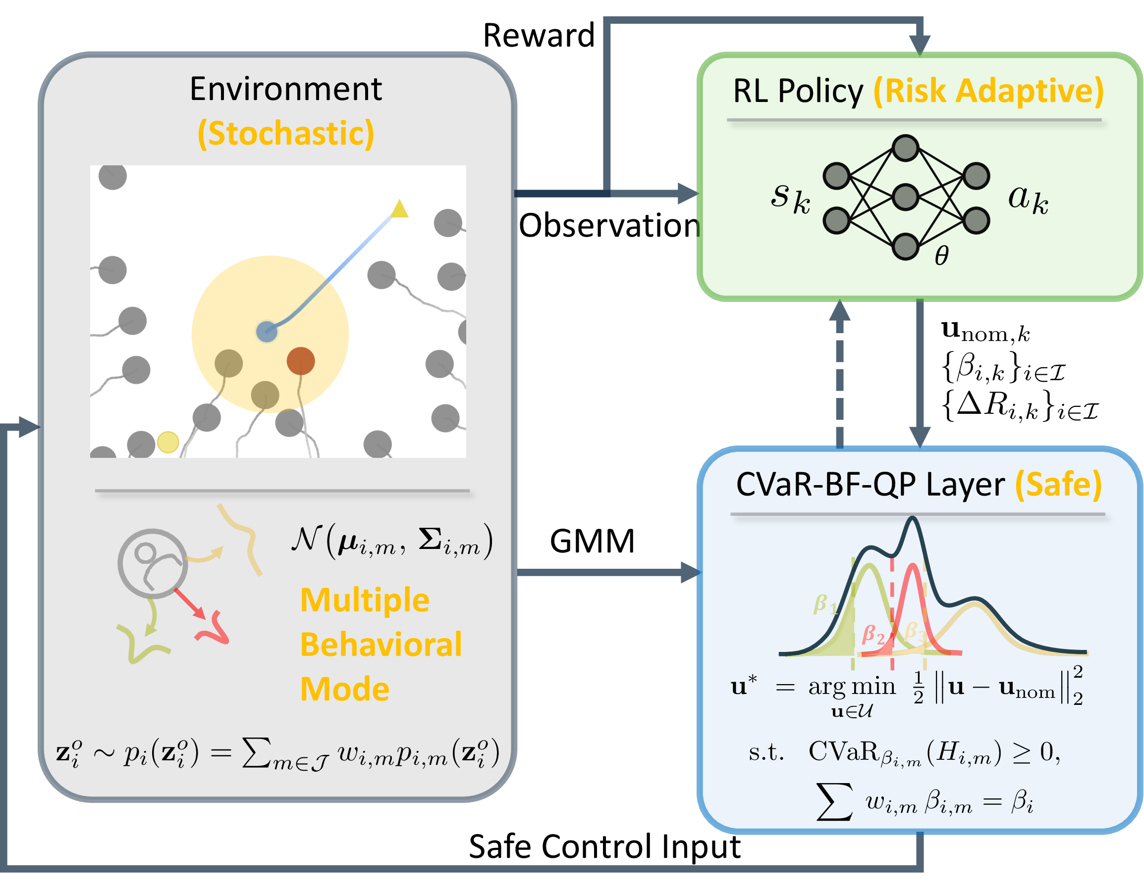
The proposed optimization in 13 can be implemented as a differentiable safety layer, enabling end-to-end policy learning while maintaining probabilistic safety guarantees. The resulting closed-loop system is modeled as a Markov decision process \((\mathcal{S},\mathcal{A},\mathcal{P},r,\gamma)\) and trained with an actor-critic algorithm. At sampling step \(k\), \(s_k\in\mathcal{S}\) is the state and \(a_k\in\mathcal{A}\) is the actor output; \(\gamma\in(0,1)\) is the discount factor. The actor policy \(\pi_\theta(a_k\mid s_k)\) produces a nominal control input and adaptive qp parameters, while the critic \(V_\omega(s_k)\) estimates the expected return.
Unlike standard rl, the action in our framework is not the final control input applied to the system. Instead, the actor outputs the adaptive parameters of the differentiable safety layer, \(a_k=\left(\mathbf{u}_{\mathrm{nom},k}, \{\beta_{i,k}\}_{i\in\mathcal{I}}, \{\Delta R_{i,k}\}_{i\in\mathcal{I}}\right),\) where \(\mathbf{u}_{\mathrm{nom},k}\) is the nominal control input, and \(\beta_{i,k}\) and \(\Delta R_{i,k}\) are the risk level and adaptive safety-margin offset for obstacle \(i\). We constrain the learned parameters to \(\beta_{i,k}\ge0\), \(\sum_{i\in\mathcal{I}}\beta_{i,k}\le\beta_{\max}\), and \(\Delta R_{i,k} \in [0,\Delta R_{\max}]\), where \(\beta_{\max}\in(0,1)\) is a user-defined total risk budget and \(\Delta R_{\max}\) is the maximum admissible safety-margin offset. The closed-loop controller consists of a neural-network actor followed by the differentiable cvarbfqp safety layer. As shown in Fig. 1, the per-step forward map is \(s_k \xrightarrow{\pi_\theta} a_k \xrightarrow{\eqref{eq:cvarbfqp}} \mathbf{u}_k^*.\)
The policy is trained with an actor-critic objective that maximizes expected discounted return. Because the cvarbfqp layer is differentiable, gradients backpropagate through the safety layer to the policy outputs \(a_k\) and the actor parameters \(\theta\). This allows the policy to optimize task performance while the cvarbfqp layer enforces a risk-aware probabilistic safety guarantee at each step.
5 Simulation↩︎
5.1 Simulation Settings↩︎
5.1.1 Environment↩︎
We evaluate our method in a crowd-navigation simulator on a \(12\,\mathrm{m} \times 12\,\mathrm{m}\) workspace with time step \(\Delta t = 0.1\,\mathrm{s}\). We train our policy using 20 dynamic obstacles, each modeled as a circle of radius \(0.4\,\mathrm{m}\), with speeds sampled from \([0.5,1.5]\,\mathrm{m/s}\) and randomized initial positions and velocities. Test results are averaged over 10 independent runs (random seeds), each evaluated on 50 episodes with randomized initial conditions.
Obstacle motion follows the Social Force Model (SFM) with uncooperative behavior. Each obstacle uses the three-mode gmm in 4 : one forward mode and two lateral-deviation modes. For simplicity, all obstacles use the same gmm, with weights \([w_1,w_2,w_3]=[0.6,0.2,0.2]\) and standard deviations \([\sigma_1,\sigma_2,\sigma_3]=[0.1,0.2,0.2]\), although the framework supports obstacle-dependent parameters. The forward mode follows the SFM direction, whereas the two lateral modes represent sudden left or right deviations. Across multiple obstacles, these modes induce combinatorial uncertainty that can accumulate over time and create tail-risk collisions absent under deterministic obstacle-motion assumptions in prior environments [12], [13]. To isolate the contribution of the cvarbfqp layer, we assume oracle access to obstacle uncertainty, i.e., the simulator provides gmm parameters that are propagated with constant-velocity prediction and then passed to the cvar computation module. In real deployments, the same interface can be provided by a learned predictor, such as Trajectron++ [24].
5.1.2 Robot Models and Barrier Functions↩︎
We consider a single-integrator (\(\dot{\mathbf{p}}=\mathbf{u}\), \(\mathbf{p}=[x,y]^\top\), \(\mathbf{u}=[v_x,v_y]^\top\)) and a unicycle (\(\dot{x}=v\cos\theta\), \(\dot{y}=v\sin\theta\), \(\dot{\theta}=\omega\), \(\mathbf{u}=[v,\omega]^\top\)), with look-ahead point \(\mathbf{p}_{\ell}=[x+\ell\cos\theta,\,y+\ell\sin\theta]^\top\) for the unicycle. Both models use \(v_{\max}=1.5\) m/s; the unicycle additionally has \(|\omega|\le\omega_{\max}=1.5\) rad/s. Collision avoidance with obstacle \(i\) (position \(\mathbf{p}_i^o\), radius \(R^o\)) uses the quadratic barrier \(h_i(\mathbf{p}_c,\mathbf{p}_i^o)=\|\mathbf{p}_c-\mathbf{p}_i^o\|_2^2-R_i^2\), with \(R_i=R_r+R^o+\Delta R_i\) and \(\mathbf{p}_c=\mathbf{p}\) (single-integrator) or \(\mathbf{p}_c=\mathbf{p}_\ell\) (unicycle) [32]. This \(h_i\) is substituted into \(H_i\) in 6 and enforced through ?? .
5.1.3 Observation and Action Space↩︎
The observation is \(o_k=[o_k^{\mathrm{rg}},o_k^{\mathrm{obs}}]\in\mathbb{R}^{8+6N_{\mathrm{obs}}}\), where \(o_k^{\mathrm{rg}}=[x_k,y_k,x_g,y_g,v_{x,k},v_{y,k},\theta_k,R_r]\) contains the robot state, goal, and radius, and \(o_k^{i}=[x_k^{o,i},y_k^{o,i},v_{x,k}^{o,i},v_{y,k}^{o,i},R^o,m_k^i]\) contains obstacle position, velocity, radius, and an activity mask indicating whether obstacle \(i\) is taken into account. We set \(N_{\mathrm{obs}}=1\), i.e., only the nearest visible obstacle within the local sensing range is included. Observations with multiple obstacles (\(N_{\mathrm{obs}}>1\)) can be encoded using, e.g., graph neural networks, and we leave this extension to future work. As defined in Section 4.3, the policy action parameterizes the differentiable safety layer. The policy outputs \(\mathbf{u}_{\mathrm{nom},k}\in\mathbb{R}^2\), corresponding to \([v_{x,k},v_{y,k}]^\top\) for the single-integrator and \([v_k,\omega_k]^\top\) for the unicycle. We set \(\beta_{\max} = 0.5\) and \(\Delta R_{\max} = 1.5(R_r+R^o)\) at each step.
5.1.4 Reward↩︎
Following [12], the reward gives \(+10\) at the goal, \(-20\) on collision, and otherwise a progress term \(r_{\mathrm{prog},k}=2(d_{k-1}^{\mathrm{goal}}-d_k^{\mathrm{goal}})\) with \(d_k^{\mathrm{goal}}=\|\mathbf{p}_k-\mathbf{p}_{\mathrm{goal}}\|_2\) and \(\mathbf{p}_{\mathrm{goal}}\) denotes the goal position. For the unicycle, we also include rotation and backward-motion penalties \(r_{\mathrm{rot},k}\) and \(r_{\mathrm{back},k}\), with \(\alpha_s, \alpha_b > 0\): \[r_{\mathrm{rot},k} = -\alpha_s(\omega_k\Delta t)^2, \quad r_{\mathrm{back},k} -\alpha_b|v_k|,\, \text{if}\,\, v_k<0.\]
5.1.5 Performance Metrics↩︎
Each test case \(j\) terminates at time \(T_j\le T_j^{\max}\) upon reaching the goal neighborhood (\(\|\mathbf{p}_j-\mathbf{p}_{\mathrm{goal}}\|_2<\delta\)) or upon collision. Let \(m_t\), \(m_s\), and \(m_c\) denote the total, successful, and collision counts, respectively, with \(\mathcal{M}\) the index set of successful cases. The episodic return is \(G_j=\sum_{k=0}^{K_j}\gamma^k r_{j,k}\) where \(K_j=\lfloor T_j/\Delta t \rfloor\), and the minimum distance is \(d_j^{\min}=\min_{t\in[0,T_j]}\min_{i\in\mathcal{I}}\bigl(\|\mathbf{p}_j(t)-\mathbf{p}_i^o(t)\|-R_r-R^o\bigr)\). We report five metrics: \[\mathrm{SR}=\frac{m_s}{m_t},\;\; \mathrm{CR}=\frac{m_c}{m_t},\;\; \mathrm{Avg.\,Ret.}=\frac{1}{m_t}\!\sum_{j=1}^{m_t} G_j,\] \[\mathrm{Traj.\,Time}=\frac{1}{m_s}\!\sum_{j\in\mathcal{M}} T_j,\;\; \mathrm{Min.\,Dist.}=\frac{1}{m_s}\!\sum_{j\in\mathcal{M}} d_j^{\min}.\]
5.2 Baselines↩︎
| Robot | Type | Policy | SR | CR | Avg. Ret. | Traj. Time | Min. Dist. |
|---|---|---|---|---|---|---|---|
| Single Integrator | Opt. | ORCA [33] | |||||
| CBF-QP [23] | |||||||
| cvarbfqp [8] | |||||||
| Adaptive-CVaR-BF [9] | |||||||
| RL | Vanilla rl | ||||||
| CrowdNav++ (const vel) [12] | |||||||
| CrowdNav++ (inferred) [12] | |||||||
| RL+Opt. | Vanilla rl + SF | ||||||
| CrowdNav++ (const vel) + SF | |||||||
| CrowdNav++ (inferred) + SF | |||||||
| BarrierNet [20] | |||||||
| Proposed | |||||||
| Unicycle | Opt. | ORCA [33] | |||||
| CBF-QP [23] | |||||||
| cvarbfqp [8] | |||||||
| Adaptive-CVaR-BF [9] | |||||||
| RL | Vanilla rl | ||||||
| CrowdNav++ (const vel) [12] | |||||||
| CrowdNav++ (inferred) [12] | |||||||
| RL+Opt. | Vanilla rl + SF | ||||||
| CrowdNav++ (const vel) + SF | |||||||
| CrowdNav++ (inferred) + SF | |||||||
| BarrierNet [20] | |||||||
| Proposed |
5pt
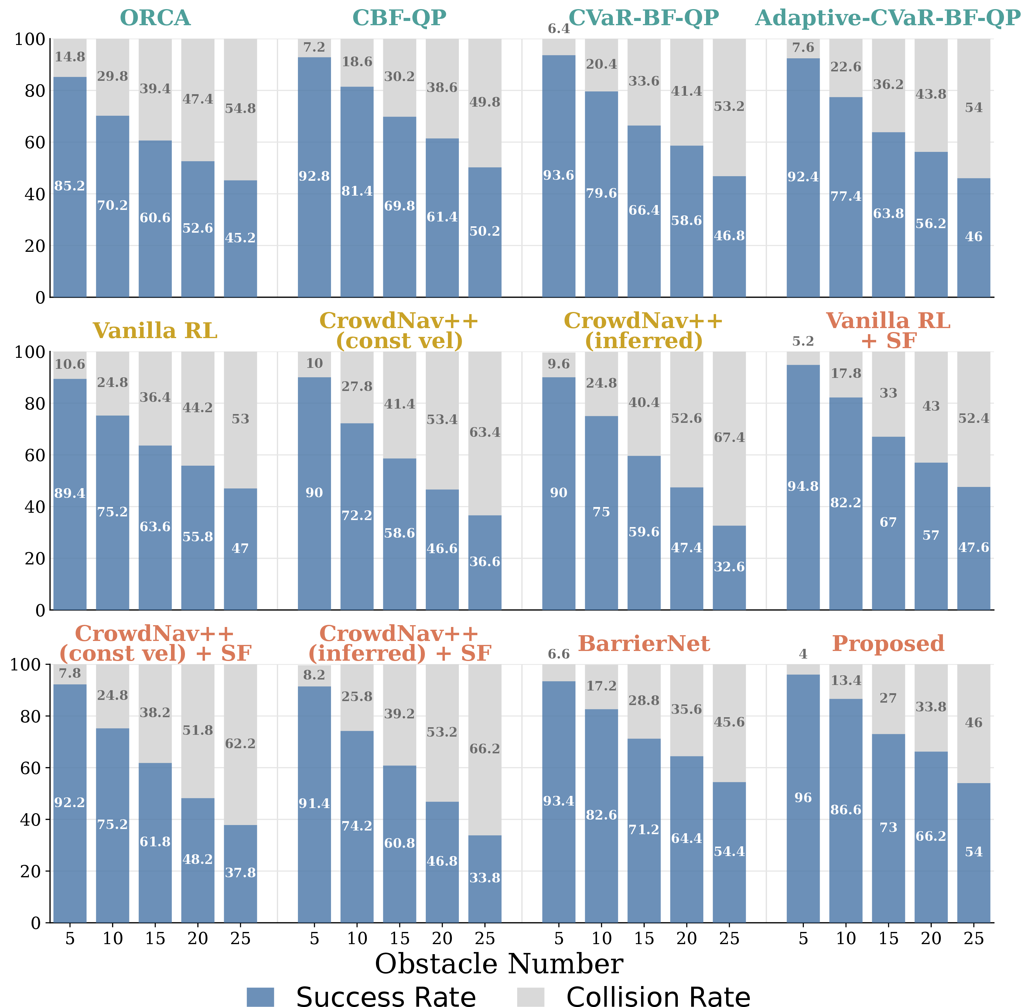
Table 1 presents comparisons with 12 baselines under 20 obstacles for both robot models: Optimization: ORCA [33] (rule-based reciprocal collision avoidance), CBF-QP [23] (deterministic safety control), cvarbfqp [8] (risk-aware safe control with a fixed risk level), and Adaptive-CVaR-BF [9] (CVaR-BF with adaptive risk tuning). RL: Vanilla rl is a standard end-to-end policy that outputs control actions directly from observations without explicit safety mechanisms. CrowdNav++ (const vel) [12] incorporates a socially aware interaction encoder, while CrowdNav++ (inferred) [12] extends this with a modular prediction of obstacle intentions. RL+Optimization: We evaluate two RL+optimization variants: post-hoc safety filtering and differentiable-layer integration. In SF baselines, nominal rl actions are projected through 13 to satisfy probabilistic safety constraints. BarrierNet [20] is trained end-to-end with a differentiable CBF-QP layer, but assumes deterministic environments without stochastic obstacle uncertainty.
In general, our method outperforms all baselines on the key metrics, achieving the highest success rate. Although the trajectory time is not the shortest, this is expected as the reward function discourages short yet impolite behaviors. Nevertheless, the proposed method remains efficient, achieving the highest return while maintaining a comfortable distance and comparable trajectory time. Here, we further distill the following key insights from our results.
Q1: How do different categories of methods perform in dynamic environments? Optimization-based methods generally struggle in highly dynamic environments because the underlying control problems can become infeasible, particularly when surrounding obstacles exhibit uncooperative behavior. In such cases, the robot cannot generate an evasive action, leading directly to collisions and lower success rates. In contrast, pure rl methods improve task performance in some cases but still exhibit relatively high collision rates without explicit safety constraints. Approaches that combine rl with optimization leverage the strengths of both and achieve more reliable overall performance.
Q2: How do different ways of integrating safety into rl affect performance? For rl methods, a post-hoc SF improves the success rate, but remains suboptimal compared to end-to-end safety integration, as it only corrects actions after learning and does not enforce safety during training, potentially degrading policy optimality. In contrast, both the proposed method and BarrierNet [20] jointly optimize the policy and safety constraints through a differentiable safety layer, enabling adaptive behavior. However, unlike BarrierNet, the proposed method explicitly models stochastic uncertainty and learns adaptive risk parameters, which leads to stronger performance.
Q3: How robust are all methods across different robot models and obstacle densities? Similar performance trends are observed for both the single-integrator and unicycle models. While all methods experience some degradation under the more challenging unicycle dynamics, this is expected due to its more constrained control dynamics. The relative performance ordering remains largely consistent. Fig. 2 further evaluates performance as the number of obstacles increases. As obstacle density grows, all methods exhibit a clear decline in success rate, reflecting the increased difficulty of navigation in dense environments. However, the rate of degradation varies across methods: the proposed method is comparatively more stable, while other methods degrade more rapidly.
5.3 Generalization↩︎
Table 2 evaluates generalization under ood scenarios in obstacle behavior, density, and size. We compare four representative methods spanning optimization-based, rl-based, post-hoc safety filtering, and differentiable-layer approaches.
Q4: How robust are different types of methods under ood cases? Vanilla rl exhibits a noticeable degradation in performance, often performing worse than optimization-based methods such as cvarbfqp. This suggests that optimization-based approaches provide greater robustness to environmental variations compared to purely learned policies. At the same time, incorporating optimization-based safety mechanisms into rl (e.g., rl with SF) significantly mitigates this degradation, recovering much of the lost performance and bringing it closer to that of optimization-based methods. However, a performance gap still remains. The proposed method consistently outperforms the baselines using SF, achieving higher success rates and returns while maintaining competitive safety. This robustness arises from the end-to-end learning of adaptive risk parameters, which enables the policy to adjust its behavior in response to changing scenarios. Additional qualitative results and video demonstrations are available on the [Paper Page].
| Case | Method | SR | Avg. Ret. | Traj. Time | Min. Dist. |
|---|---|---|---|---|---|
| I | cvarbfqp | ||||
| rl | |||||
| rl + SF | |||||
| Proposed | |||||
| cvarbfqp | |||||
| rl | |||||
| rl + SF | |||||
| Proposed | |||||
| cvarbfqp | |||||
| rl | |||||
| rl + SF | |||||
| Proposed |
2.8pt
5.4 Computational Efficiency↩︎
We benchmark our closed-form cvarbfqp against a sampling-based baseline [9] on an Apple M4 CPU (single thread), as shown in Fig. 3. The per-step cost is \(\mathcal{O}(N_{\mathrm{obs}} M)\) versus the baseline’s \(\mathcal{O}(N_{\mathrm{obs}} N \log N)\), where \(N\) is the number of Monte-Carlo samples drawn from the gmm to estimate cvar. Remarkably, the measured per-step computational time stays nearly flat across the tested \(N_{\mathrm{obs}}\) range, confirming that our closed-form cvar formulation is tractable and well suited to real-time control.
6 Conclusions↩︎
This paper presented an end-to-end risk-adaptive framework for safe robot navigation in uncertain dynamic crowds. By coupling an rl policy with a differentiable cvarbfqp safety layer under a gmm obstacle-motion uncertainty model, the method jointly learns nominal control input, risk level, and safety margin, enabling adaptive conservatism with probabilistic safety guarantees. Experiments with both single-integrator and unicycle robots show that the method maintains safety while improving efficiency relative to optimization-based, rl-based, and integrated rl with optimization methods. The gains remain evident in ood cases: under the high obstacle density case (30 obstacles) with the single-integrator robot, the proposed method improves the success rate, corresponding to an approximately 30.8% relative improvement over vanilla rl. Future work will extend this to encode multiple surrounding obstacles jointly via graph neural networks, and to incorporate multi-step predictive safety constraints for longer planning horizons.
