Foundation Models for Credit Risk Prediction: A Game Changer?
May 18, 2026
Abstract
Predictive models play a pivotal role in credit risk management, guiding critical decisions through accurate estimation of default probabilities and losses. Their performance influences the profitability of lending operations and the stability of the financial system. The relevance of predictive modeling has generated extensive interest in credit risk research, with numerous studies introducing new modeling techniques. Large-scale benchmarking studies complemented these endeavors by periodically consolidating the state-of-the-art and systematically uncovering the merits and demerits of methodological advancements. Today, quasi-standards such as a gradient-boosting model for prediction, often paired with a SHAP explainer, have emerged for specific contexts. However, the continuous improvement of risk models and modeling practices remains a top priority.
Concurrently, the rapid advancements in AI, most notably through large language models, have disrupted predictive modeling paradigms in many fields. Foundation models, pretrained on extensive datasets from diverse domains, have demonstrated remarkable performance by leveraging prior knowledge acquired during pretraining. While prevalent in natural language processing and computer vision, foundation models specifically designed for tabular data have only recently emerged and may hold great potential for credit risk management. We conjecture that pretraining on out-of-domain data is particularly beneficial in small-data settings, such as SME lending or managing specialized corporate portfolios. More technically, foundation models may help address longstanding credit-scoring challenges, including low default portfolios or class imbalance. However, the actual value of foundation models for credit risk prediction remains an open question.
This paper focuses on recently proposed foundation models for tabular data. We benchmark these models against a broad set of competitors, including established and advanced machine learning techniques in two core prediction tasks: PD and LGD modeling. Our evaluation extends on the design of previous benchmarking studies, encompassing various datasets, performance indicators, and experimental conditions to clarify pretraining benefits across relevant risk modeling challenges. We find that tabular foundation models generally perform best across datasets and tasks in comparison with state-of-the-art alternatives. Moreover, we find that tabular foundation models offer significant improvement in predictive performance when the size of the dataset in terms of number of observations grows smaller. These results are remarkable, since the tabular foundation models are tested out-of-the-box, without applying any hyperparameter tuning, ensuring ease of use and mitigating the computational costs associated with employing foundation models.
1 Introduction↩︎
Foundation models are large-scale machine learning systems that have been trained on vast and heterogeneous corpora and, as such, acquire representations and inductive biases that transfer to a wide range of downstream tasks (possibly after fine-tuning through further training on application-specific data) [1]. Foundation models have transformed domains such as natural language processing (NLP) and computer vision. In NLP, large language models such as GPT-4 have redefined the state of the art in tasks such as next-word prediction and text generation [2]; in computer vision, models such as CLIP [3] and diffusion-based generators have enabled zero-shot classification—classification of previously unseen classes or tasks without task-specific training—and high-fidelity synthesis that were previously out of reach [4]. These advances exemplify a shift away from traditional model-training approaches towards developing and using general-purpose models with broad applicability and, potentially, improved task performance.
Analogous developments have recently reached tabular data—the workhorse format of credit risk analytics. Tabular learning differs markedly from unstructured domains due to heterogeneous feature types, disparate scales, and dataset-specific semantics that have historically impeded knowledge transfer. Tree-based ensembles such as gradient boosting machines (GBMs) have long dominated tabular benchmarks, consistently outperforming deep learning alternatives in extensive comparative studies [5]–[7]. Prior-Data Fitted Networks (PFNs), however, extend the foundation model idea to the tabular setting by pretraining on large numbers of synthetic datasets drawn from priors over data-generating processes [8], [9]. At inference, a PFN processes an entire dataset, including labeled and unlabeled instances, in a single forward pass and outputs predictive distributions without further training or tuning.
This paper examines whether the foundation model paradigm benefits credit risk modeling. Credit risk management is critically dependent on accurate predictions of risk parameters, notably the probability of default (PD) and the loss given default (LGD). Improvements in predictive accuracy directly affect capital calculation, allocation, and portfolio steering under the Basel framework, provisioning under IFRS 9, and risk-adjusted pricing. If PFNs can deliver competitive accuracy without task-specific training, they could simplify model development, monitoring, and maintenance, reduce operational costs, and improve time-to-model, especially in small-data contexts.
PFNs promise advantages that are particularly relevant for credit risk modeling practice. First, as zero-shot forecasters, they avoid repeated hyperparameter tuning and retraining across tasks and portfolios. This property is attractive for portfolios with limited data availability, such as low-default portfolios, specialized corporate segments, or new credit products. Second, PFNs could enable a consistent modeling approach across risk parameters (PD, LGD, and potentially exposure at default, EAD), thereby benefiting governance by simplifying validation, monitoring, and model risk management. From a supervisory perspective, cross-parameter consistency within financial institutions and methodological uniformity across institutions may reduce the burden of model review. Third, by combining broad synthetic pretraining with in-context learning on institutional data, PFNs may temper historical biases embedded in local datasets and thereby support fairer, more inclusive decision making [10]–[12].
Despite this potential, there are reasons for caution. Credit risk modeling presents specific challenges—severe class imbalance, heterogeneous borrower populations, economic non-stationarities, and regulatory constraints—that may not be fully addressed by current tabular foundation models (TFMs). Moreover, a systematic evaluation of PFNs for credit risk prediction has been lacking. While anecdotal evidence suggests strong performance on small datasets, it remains unclear whether PFNs can consistently match tuned baselines across diverse credit portfolios and targets.
We address this gap with an extensive empirical benchmark. We compare PFNs against classical and advanced machine learning methods on a collection of PD and LGD datasets that vary in size, dimensionality, and label characteristics. Our evaluation protocol follows the benchmarking tradition in credit scoring, uses cross-validation, and assesses a comprehensive set of performance metrics. We further conduct statistical tests to assess the significance of algorithm comparisons across datasets. As a by-product, our benchmark provides the first credit-risk assessment, to the best of our knowledge, of several recent non-PFN deep learning algorithms for tabular data. The remainder is organized as follows. Section 2 reviews credit risk modeling and recent advances in deep learning for tabular data. Section 3 introduces PFNs and their Bayesian interpretation. Section 4 details the experimental setup in terms of datasets, preprocessing steps, the evaluated learners, and the evaluation protocol. Section 5 presents empirical results and discusses practical implications. Section 6 concludes.
2 Literature review↩︎
This paper contributes to the empirical credit scoring literature by providing original results concerning the predictive performance of TFMs in two crucial prediction applications, PD and LGD modeling. In doing so, the paper draws on a large body of prior work on credit risk prediction and extends it by introducing a new family of predictive methods. Beyond credit risk and, more generally, financial applications, the paper also draws on prior work on deep learning for tabular data, which paved the way for the recently introduced PFNs, which are central to this study. Below, we review prior work in these two fields and elaborate on our contributions.
2.1 Credit risk modeling↩︎
Credit risk refers to the potential loss arising from a counterparty’s failure to meet contractual obligations [13]. In retail and wholesale banking, risk models quantify key risk parameters used for pricing, capital, provisioning, and portfolio management: the PD, which estimates the likelihood of a borrower defaulting over a fixed horizon, and the LGD, which measures the proportion of exposure not recovered if default occurs. In both PD and LGD modeling, predictive accuracy is key to the efficiency and effectiveness of credit risk management [6], [14], [15].
Better predictions directly translate into improved capital efficiency (e.g., when estimating expected loss under the Basel Accord’s IRB approach), more precise and timely provisioning under IFRS 9 through improved estimation of lifetime expected credit losses, reduced impairments, and better pricing decisions [16]. Regulators likewise emphasize the discriminatory power and calibration of scorecards, for example through backtesting, monitoring stability, and validation requirements.
Aiming to unlock financial rewards from more accurate predictions, the community routinely assesses the potential of new prediction methods and proposes methodological adjustments tailored to characteristic modeling challenges. For PD, these challenges include class imbalance [17]–[20], reject inference [21], [22], economic cycle dependency [23]–[26], or non-linear interactions in borrower behavior [27], [28]. Compared with PD prediction, fewer studies have considered LGD modeling [29]–[31], which may be due to the limited public availability of LGD datasets. Public datasets that are frequently used in LGD modeling research include the LendingClub and Freddie Mac datasets [32], [33], which provide sufficient information to approximate LGD. Given the characteristic bi-modal shape of real-world LGD distributions, arising, for example, from mixed portfolios comprising both secured and unsecured loans, many studies recommend multi-stage models [34]–[36]. Dynamic models that explicitly recognize capital inflows and outflows throughout the workout period [37] are another popular research topic in the LGD literature, often involving survival modeling [38].
Given the prevalence of machine learning and advanced predictive methods in the credit scoring literature, several benchmarking studies have periodically consolidated the state of the art by applying an arsenal of statistical and machine learning methods across multiple datasets, performance metrics, and experimental conditions. Prominent examples include [5], [6], [14], [39] and [15], [40], for PD and LGD prediction, respectively. Closely connected to comparing the predictive performance of alternative methods is the question of how to properly assess predictions. Several attempts have been made to connect the accuracy of model predictions to profitability and other measures of business impact [41]–[43]. While quantification of business impact is more developed in PD modeling, some studies have pursued similar goals in the context of LGD [44].
Conditional on the availability of suitable indicators of a risk model’s business impact, the predictive models themselves can be optimized for cost-minimization [45] or profit maximization [46]–[49]. Beyond the actual risk model, other stages in the modeling pipeline can be optimized for cost/profit objectives. For example, [50], [51] introduce techniques for profit-oriented feature selection. Also targeting the input data of predictive models, recent work aims to extract information from borrower networks that standard methods relying on the IID assumption would fail to capture. Using methods from geospatial econometrics, related studies have, for example, established correlations between default events across geographical neighborhoods [52], [53]. More generally, graph-based algorithms, such as graph neural networks (GNNs), facilitate the processing of comprehensive dependency structures, providing modelers with considerable freedom in how to design an influence network.
[54] pioneered the use of multilayer network analysis in credit-risk modeling, showing that borrower connections can provide substantial predictive gains. This line of work has since developed towards graph-based and graph neural network approaches for credit-risk prediction [55], [56]. The pursuit to incorporate auxiliary information in risk models beyond what classical scorecards embody has also inspired scholars to systematically explore novel sources of data, including social media postings [57], psychometric data [58], and, perhaps most prominently, textual data [59]–[61]. A distinctive advantage of such alternative data is that it may facilitate accurate risk assessment and, by extension, lending to thin-book clients whose limited credit history may otherwise exclude them from accessing financial services [10].
Facing increasing concern related to the omnipresence of advanced, AI-based, decision models in lending—and beyond—much recent work concentrates on explainable AI (XAI) techniques to ensure that the mechanisms underlying such models are well-understood [62]. Model explainability is a regulatory imperative and prerequisite for achieving higher-level objectives, including robustness, safety, and fairness [63]. Recent work on XAI for credit risk examines the interplay between ML-based scorecards and XAI tools in general [16], the robustness of explanations [64], or the moderating effect of longstanding challenges, such as class imbalance [65]. Benefiting from its strong theoretical foundations in cooperative game theory, the SHAP framework for additive feature attribution has gained considerable popularity in credit risk and may be considered a quasi-standard [66], [67]. Unlike SHAP, which decomposes a model’s prediction, be it right or wrong, [68] introduces an interesting challenger approach that inherits the same theoretical underpinnings but decomposes a scorecard’s predictive performance. The corresponding insights might be even more meaningful to decision-makers as, on one hand, performance statistics are easier to interpret than predictions, and, on the other hand, knowing which features drive performance provides directly actionable insights to improve the model. Apart from techniques to explain otherwise opaque machine learning models, several studies devise new, intrinsically interpretable learning algorithms and demonstrate that these often avoid sacrificing (much) predictive accuracy. Representative examples include tree-based approaches [69], [70] , generalized additive models [71], and interpretable deep learning techniques [72], [73].
Regulatory frameworks governing the use of AI in consumer-facing applications, such as the EU AI Act, the EU GDPR, and recent revisions to the Basel capital accord, require financial institutions to demonstrate that their risk models are not only explainable but also free from discriminatory bias against historically disadvantaged groups. Seminal papers provide evidence that scorecards exhibit such biases and that machine-learning-based approaches are especially vulnerable [74], [75]. Focusing on retail lending decisions, [11] systematically analyze available statistical indicators of algorithmic fairness and algorithms to mitigate disparate impact in the machine learning pipeline for their suitability in credit scoring. [76] introduce a powerful tool to test a given scorecard for algorithmic bias, enabling lenders to verify compliance (or the lack thereof) with regulatory requirements.
In summary, it is clear that machine learning and AI play a pivotal role in credit risk modeling. They continuously supply novel technologies that aid lenders in their quest for more effective, efficient, and ultimately profitable decision models that are also compliant with regulation.
This paper contributes to the empirical credit risk modeling literature. Although we focus on established classification and regression settings for PD and LGD modeling, respectively, our goal extends beyond assessing yet another prediction method. Instead, we evaluate a novel paradigm for risk prediction: the use of tabular data foundation models for zero-shot forecasting. Adopting a zero-shot forecasting method to support lending operations entails a fundamental shift in established risk modeling practices, moving from task-specific model training and calibration to the use of pretrained foundation models and in-context learning. Given these consequences and the prevalence of predictive modeling in credit risk, we consider a holistic evaluation of the new paradigm in canonical risk modeling tasks imperative.
2.2 Deep learning for tabular data↩︎
The study follows prior work and established industry practices of approaching PD and LGD modeling as classification and regression problems, respectively. Consequently, we use supervised machine learning algorithms for labeled tabular data [13].
Deep learning (DL) has revolutionized various data modalities and represents the uncontested state-of-the-art in NLP and computer vision, to name only a few [77]. Given that natural language is a specific type of sequential data, it is not surprising that DL has also become a go-to method for time series forecasting [78]. With respect to cross-sectional tabular data, however, classic ML methods, particularly gradient-boosted trees (GBM), may be considered the de facto standard. Benchmarking experiments have shown the superiority of GBM over DL-based approaches in that the former often provide more accurate predictions at lower computational costs and/or with less need for hyperparameter tuning [79], [80]. [81] contextualize this finding by elaborating on the specific conditions (e.g., dataset characteristics) when DL excels. Considering PD modeling, however, [6] argue that the potential of DL lies in unlocking non-standard data sources (e.g., text) to augment risk models rather than serving as a vehicle for model estimation. For model estimation, [6] find that GBM-type approaches excel, which echoes earlier benchmarking results.
We argue that the [6] study represents the credit risk modeling space well, in particular for tabular data. DL has provided excellent results in use cases involving semi-structured and unstructured data modalities [82], such as text data or networks [55], [60], and settings that employ time-varying covariates [72], [83], whereas GBM-type algorithms, often paired with a post-hoc XAI approach, remain the standard solution when the goal is to develop highly accurate risk scorecards.1
The unmatched success of DL in unstructured data settings stands in sharp contrast to its moderate performance on tabular data, which has inspired much recent work aimed at closing the performance gap with GBM-type approaches. Given that the transformer architecture was instrumental to the success of DL in unstructured data settings and that it relies on the attention mechanism, unlocking the power of attention for tabular data was a natural next step. The work by [84], introducing FT-Transformer, may be seen as a seminal paper paving the way for more advanced DL-based tabular data models. The authors demonstrate effective ways to utilize attention when working with tabular data, which is essential because it enables models to flexibly capture heterogeneous feature interactions common in tabular domains. Unlike convolutional or recurrent layers, attention can dynamically weight dependencies across diverse variables, reducing the need for manual feature engineering. Building on FT-Transformer, subsequent work has refined attention variants for tabular data, confirming its role as a central design principle in closing the performance gap with GBMs [85].
[86] provide a comprehensive survey of DL models for tabular data and their evolution. The authors identify three main evolutionary stages of deep tabular learning. The first stage includes approaches similar to FT-Transformer, which are trained and evaluated within a single distribution and focus on feature-level encoding, sample-level interactions, and objective-driven regularization [87], [88]. These approaches introduced innovations such as feature tokenization, attention-based feature selection, and inter-sample retrieval, but their generalization remained limited to the dataset at hand.
The second stage, transferable models, extended this paradigm by pre-training on one or multiple source datasets and fine-tuning on downstream tasks. Such models seek to overcome heterogeneity in feature and label spaces, often leveraging self-supervised objectives or language-model-inspired pretraining to enable cross-dataset knowledge transfer [89]–[91]. For example, TabLLM serializes tabular data by integrating feature names into text and combining them with task descriptions, which enables approaching tabular prediction tasks as language generation problems and, thus, the use of large language models in a few-shot mode [92].
The most recent, third stage is marked by foundation models for tabular data, which provide zero-shot capabilities across diverse domains without the need for fine-tuning. Within this category, Prior-Data Fitted Networks (PFNs) stand out as a pioneering approach that harnesses synthetic pretraining and in-context learning with transformers to deliver robust generalization across a wide range of tabular problems [93]. PFNs approximate Bayesian inference by pretraining on synthetic datasets generated from, for example, structured causal models, thereby endowing the transformer with a learned prior that enables strong in-context learning capabilities [94]. Introducing TabPFNv2, [95] is a landmark paper demonstrating the generality, predictive capability, and scalability of a PFN-based zero-shot learner. The authors conduct comprehensive empirical comparisons to demonstrate that their approach matches the performance of GBM algorithms across a large set of regression and classification problems. Given that in-context learning requires a PFN to process an entire dataset in a single forward pass, the scalability of TabPFNv2 remains limited to moderately sized tables (e.g., 10,000 observations). Addressing this bottleneck is the subject of current research [96], [97].
The three stages illustrate how the field of deep tabular learning has shifted from approaches that adopt the classic ML paradigm of training task-specific models to increasingly versatile architectures, which mimic the generality of contemporary AI models. It is this generality, achieved through in-context learning and pretraining on large out-of-domain data collections, which we consider a paradigm shift with potentially far-reaching implications for credit risk modeling. This prospect, as well as the cautionary remarks of [98], who argue that the impressive results of PFNs in laboratory environments may give a false impression of how easy it is to use corresponding methods in practice, motivate the focal study, in which we undertake a comprehensive empirical evaluation of PFNs for credit risk modeling.
We acknowledge that our work does not advance deep tabular data learning methodology. Instead, we aim to contribute original empirical insights into how that field’s latest innovations compare with established domain standards in credit risk modeling. Such evidence is valuable because the evaluation of PFNs has not moved beyond the standard benchmarking datasets routinely used in machine learning. These dataset collections are comprehensive and aim to be general by combining data from various fields. While clearly effective for demonstrating the potential of a new approach, decision-makers may appreciate targeted results that reflect the characteristics of their domain. Thus, our study provides a critical test of whether PFNs can move from promising benchmarks to delivering real impact in credit risk modeling.
3 Prior-data fitted networks (PFNs)↩︎
PFNs are pretrained models that approximate the Bayesian posterior predictive distribution at inference time [94]. While applicable to various data types, TabPFN, a specific type of PFN, has shown great potential as a foundation model for tabular prediction [93]. The core idea is to encode prior beliefs about likely relationships between inputs and outputs by defining a prior over data-generating processes, which are functions that map features to targets. Next, TabPFN repeatedly samples functions from this prior to generate synthetic datasets, which are subsequently used as training examples. Using these synthetic datasets as training points, a permutation-invariant transformer architecture is trained to map observed training pairs and features to posterior predictive distributions over the targets. Through this training, the model learns to approximate the posterior predictive distribution that is implied by the defined prior, conditioned on the observed data. Conceptually, TabPFN amortizes Bayesian inference: the computationally expensive inference is learned once during pretraining, so that inference on a new dataset reduces to a single forward pass.
Formally, consider a tabular dataset \(\mathcal{D} = \{(x_i, y_i)\}_{i=1}^n\) with features \(x_i \in \mathbb{R}^d\) and targets \(y_i\) (binary for PD, continuous and bounded for LGD). TabPFN receives as input both labeled context examples and unlabeled query examples and outputs predictive distributions \(p(y \mid x, \mathcal{D}_{\mathrm{context}})\) over the target. During pretraining, synthetic tasks are generated by sampling from a prior over joint distributions \(p(x,y)\), including mechanisms that induce missingness, correlations, and noise features, thereby ensuring that TabPFN encounters a diverse range of realistic tabular structures. The model is trained to minimize a proper scoring rule, e.g., log-loss for classification or a suitable continuous target loss for regression, over held-out query examples from each synthetic dataset.
A Bayesian interpretation arises because TabPFN aims to learn a mapping that approximates the posterior predictive distribution \(p(y \mid x, \mathcal{D}_{\mathrm{context}})\) that is implied by the training prior over data-generating processes [94]. In the limit of infinite synthetic data and capacity, TabPFN converges to Bayes-optimal predictions for tasks drawn from the prior. In practice, expressivity, prior misspecification, and optimization constraints introduce approximation errors, causing deviations from the true Bayesian posterior distribution. Nevertheless, empirical results indicate strong performance, especially on small datasets where traditional learners are prone to overfitting or require heavy regularization [9].
Two properties are particularly salient for credit risk modeling. First, TabPFN provides zero-shot predictions on new datasets; it does not require any task-specific training or hyperparameter tuning, as inference reuses the pretrained network. Second, TabPFN can process tabular datasets with varying numbers of features and examples using cell embeddings and masked attention, allowing the same pretrained network to operate across heterogeneous structures. This flexibility is essential for lenders, as they must model risk exposure across heterogeneous credit portfolios, drawing on datasets that vary substantially in size, dimensionality, and distributional characteristics.
4 Experimental design↩︎
4.1 Data↩︎
We evaluate PFNs for PD and LGD estimation, corresponding to classification and regression tasks, respectively. Our experiments use both public and proprietary datasets spanning retail and small-business portfolios. Tables 1 and 2 summarize the key characteristics of the PD and LGD datasets, respectively, including sample size, dimensionality, minority class proportion, and data origin.
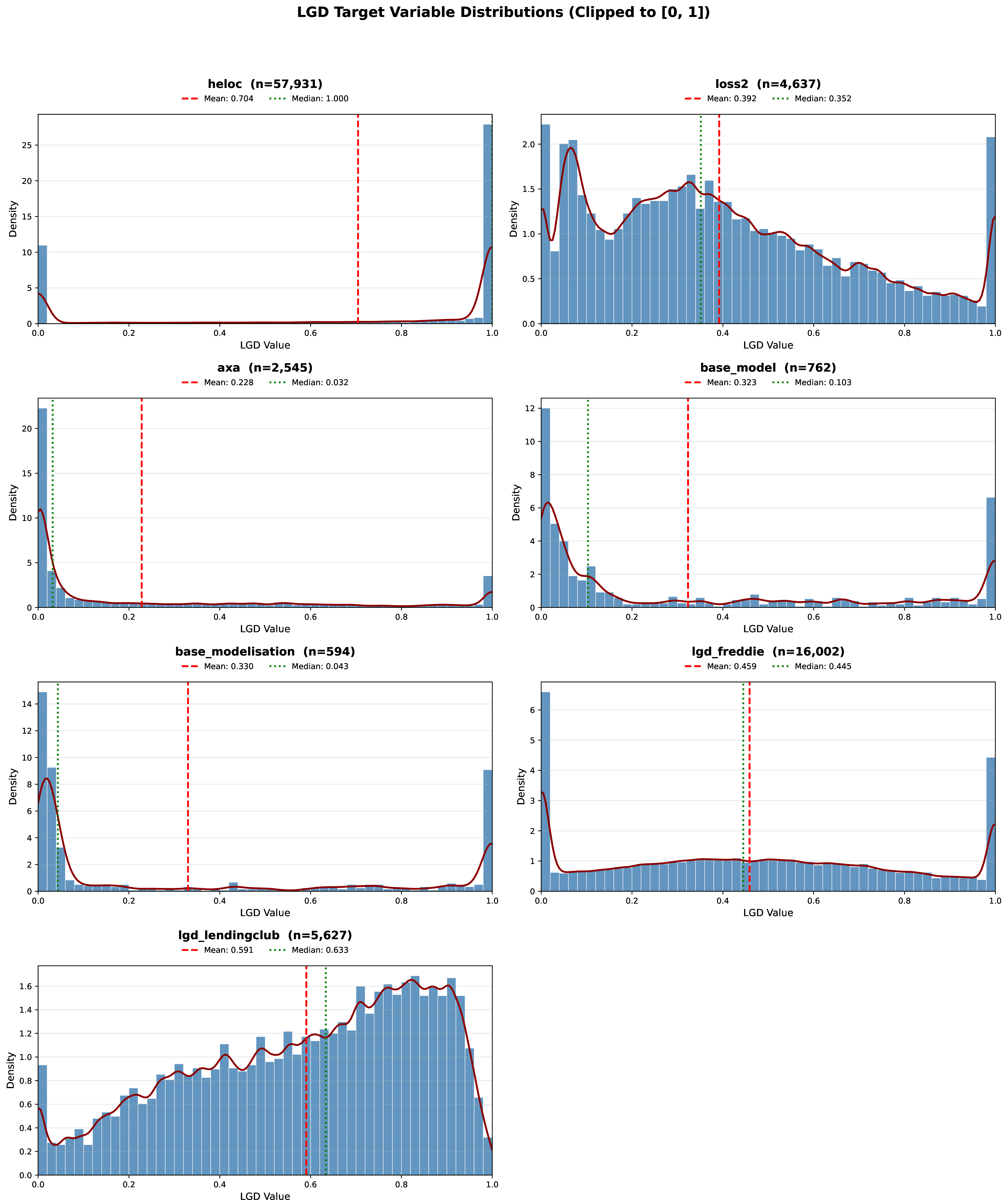
Our datasets vary substantially in the number of observations, the number of features, and the distribution of the target variable. For PD, the default rate differs substantially across portfolios, ranging from approximately \(6.7\%\) to \(40.0\%\) (mean \(\approx 22.1\%\), median \(\approx 22.4\%\)). For the LGD datasets, the target variable exhibits a typical bimodal, zero-one-inflated distribution across most datasets, as reported in [15]. The bimodality of the LGD distribution arises due to, on the one hand, the high risk of losing the entire outstanding amount in the event of default for unsecured exposures, resulting in an LGD value equal to or close to \(100\%\), while for secured loans, on the other hand, the full outstanding amount at time of default is often recovered, resulting in an LGD value equal to or close to \(0\%\). Figure 1 visualizes the distribution of the target variable in the LGD datasets.
| ID | Dataset name | Observations | Variables | Minority % | Source |
|---|---|---|---|---|---|
| PD1 | GMSC (Give Me Some Credit) | 150,000 | 10 | \(6.7\%\) | Kaggle |
| PD2 | Taiwan Credit Card | 30,000 | 23 | \(22.1\%\) | UCI |
| PD3 | Vehicle Loan | 233,154 | 35 | \(21.7\%\) | Kaggle (LTFS) |
| PD4 | LendingClub (PD) | 9,578 | 13 | \(16.0\%\) | LendingClub |
| PD5 | Myhom | 7,000 | 8 | \(40.0\%\) | Kaggle |
| PD6 | Hackerearth | 532,428 | 35 | \(23.6\%\) | Hackerearth |
| PD7 | Cobranded | 80,000 | 47 | \(24.6\%\) | Kaggle |
| PD8 | German Credit | 1,000 | 20 | \(30.0\%\) | UCI |
| PD9 | Bank Status | 100,000 | 16 | \(22.6\%\) | Proprietary |
| PD10 | Thomas | 1,225 | 14 | \(26.4\%\) | [99] |
| PD11 | Loan Default | 105,471 | 759 | \(9.3\%\) | Proprietary |
| PD12 | Home Credit | 307,511 | 120 | \(8.1\%\) | Kaggle |
| PD13 | HMEQ | 5,960 | 12 | \(19.9\%\) | SAS |
| PD14 | MicroFinance | 158,700 | 2,986 | \(37.8\%\) | [22] |
| ID | Dataset name | Observations | Variables | Source | |
|---|---|---|---|---|---|
| LGD1 | HELOC | 57,931 | 8 | FICO | |
| LGD2 | Loss2 | 4,637 | 52 | – | |
| LGD3 | AXA | 2,545 | 2 | AXA | |
| LGD4 | Base Model | 762 | 202 | – | |
| LGD5 | Base Modelisation | 594 | 256 | – | |
| LGD6 | Freddie Mac (LGD) | 16,002 | 20 | Freddie Mac | |
| LGD7 | LendingClub (LGD) | 5,627 | 17 | LendingClub |
4.2 Data preprocessing↩︎
We apply a consistent preprocessing pipeline across all datasets to ensure comparability, implemented in TALENT [100], a unified benchmarking framework for tabular learning that standardizes data handling, method integration, and evaluation across a broad set of algorithms. All preprocessing parameters are learned exclusively from the training data of each cross-validation fold (cf. infra) and applied to the validation and test partitions of the corresponding cross-validation iteration, thereby avoiding data leakage. We impute missing values in numerical features with their median, and introduce a novel category level for missing values in categorical features. We subsequently encode these as integer indices for methods that support categorical inputs natively, or via one-hot encoding for methods that require real-valued inputs; the encoding policy is specified and enforced per method within TALENT. We apply normalization in a method-specific manner: all numerical variables are standardized to zero mean and unit variance, except for TFMs (TabPFN, TabPFNv2, TabPFN-Real, MITRA, TabICL), which operate on raw, non-normalized inputs.
4.3 Benchmarking protocol↩︎
We compare a diverse panel of competitive learners, ranging from classical statistical methods to state-of-the-art deep tabular architectures. For PD, we compare 29 different methods, including foundation models (TabPFN, TabPFNv2, TabPFN-Real, MITRA, and TabICL), several classical methods, particularly tree-based ensembles (XGBoost, LightGBM, CatBoost), and a wide array of deep learning models, including transformers (e.g., FT-Transformer, ExcelFormer) and specialized architectures like TabNet and TabM.
For LGD, the benchmark comprises 22 methods, including foundation models that support regression at the time of evaluation (TabPFNv2), classical regression baselines, gradient-boosting approaches, and advanced deep learning architectures such as ModernNCA, ResNet, and PTARL. Table 3 summarizes the full set of methods considered across both tasks.
| Method Name | PD | LGD |
|---|---|---|
| Foundation Models | ||
| TabPFN | ✔ | |
| TabPFNv2 | ✔ | ✔ |
| TabPFN-Real | ✔ | |
| MITRA | ✔ | |
| TabICL | ✔ | |
| Tree Boosting | ||
| CatBoost | ✔ | ✔ |
| LightGBM | ✔ | ✔ |
| XGBoost | ✔ | ✔ |
| Deep Tabular (Transformers) | ||
| FT-Transformer (ftt) | ✔ | ✔ |
| AutoInt | ✔ | ✔ |
| ExcelFormer | ✔ | ✔ |
| AMFormer | ✔ | |
| T2G-Former | ✔ | ✔ |
| PTARL | ✔ | |
| Deep Tabular (MLP & Specialized) | ||
| MLP | ✔ | ✔ |
| ResNet | ✔ | |
| SNN | ✔ | |
| RealMLP | ✔ | ✔ |
| MLP-PLR | ✔ | ✔ |
| DANets | ✔ | |
| SwitchTab | ✔ | |
| TabNet | ✔ | ✔ |
| DCN2 | ✔ | ✔ |
| TabM | ✔ | ✔ |
| TANGOS | ✔ | ✔ |
| ModernNCA | ✔ | |
| Classical ML | ||
| Logistic Regression | ✔ | |
| Linear Regression | ✔ | |
| K-Nearest Neighbors (KNN) | ✔ | ✔ |
| Random Forest | ✔ | ✔ |
| Support Vector Machine (SVM/SVR) | ✔ | ✔ |
| Naive Bayes | ✔ | |
| Nearest Class Mean (NCM) | ✔ |
Performance is evaluated on the held-out test partition within a five-fold cross-validation scheme. We tune hyperparameters on a validation split comprising 20% of the training fold by maximizing the area under the ROC curve (AUC) for PD models, and by minimizing the mean squared error (MSE) for LGD models. These objectives are used to select hyperparameters within each fold. Hyperparameter optimization is performed independently in each fold using the Optuna framework [101] with up to 20 trials.
For PD modeling, we consider a diverse set of metrics that evaluate discrimination, calibration, and decision performance, including AUC, Gini, KS (Kolmogorov-Smirnov), Brier score, LogLoss, and Average Precision (PR-AUC). We also report threshold-based metrics, including Accuracy, Balanced Accuracy, F1-score, Precision, Recall, and the Matthews Correlation Coefficient (MCC). To compute these, we convert model-estimated PD probabilities to labels using an optimal threshold determined by maximizing the F1-score on the validation set.
For LGD prediction, we measure forecast accuracy in terms of \(R^2\), MSE, RMSE, and MAE, as well as MedAE, Max Absolute Error, Pearson and Spearman correlation coefficients, and Explained Variance. All LGD predictions are clipped to the \([0, 1]\) interval before metric calculation to ensure they remain within the logical bounds of loss given default.2
4.4 Statistical analysis↩︎
Principles for comparing learners across datasets in a statistically sound way have been established by [102]. Recent machine learning benchmarks advocate modifications, involving a pairwise comparison of learners’ performance using a Student’s \(t\)-test (e.g., comparing AUCs over datasets or cross-validation folds) followed by Holm’s step-down adjustment to control the family-wise error rate at \(\alpha=0.05\) in multiple comparisons [85], [100]. We adopt a similar approach, yet we replace the \(t\)-test with the Wilcoxon signed-rank test [103], a non-parametric alternative that does not assume normality of performance differences and accounts for both the direction and magnitude of differences across datasets.
We further summarize the likelihood that a given method “wins” a dataset using the probability of achieving maximum accuracy (PAMA), computed as the relative frequency of a learner to achieve the top performance (in a given metric) across all cross-validation splits and datasets [104]. Whereas the classic statistical tests assess whether performance differences between learners are significant, PAMA highlights the practical dominance frequency, thereby complementing the analysis of differences in learners’ performance and their statistical significance.
5 Results and discussion↩︎
The empirical results comprise estimates of predictive performance across learning algorithms, datasets, and cross-validation folds, using various evaluation metrics.
5.1 PD modeling↩︎
Figure 2 reports the average performance of classification methods in terms of AUC, across the five folds of all PD datasets. A first observation is that TabICL, one of the foundation models considered here, achieves the best performance overall. Although the observed performance differences are small in absolute terms, it is notable that—without any training or hyperparameter optimization—a TFM outperforms widely credited boosting-based ensembles, which may be considered a de facto standard in credit risk modeling.
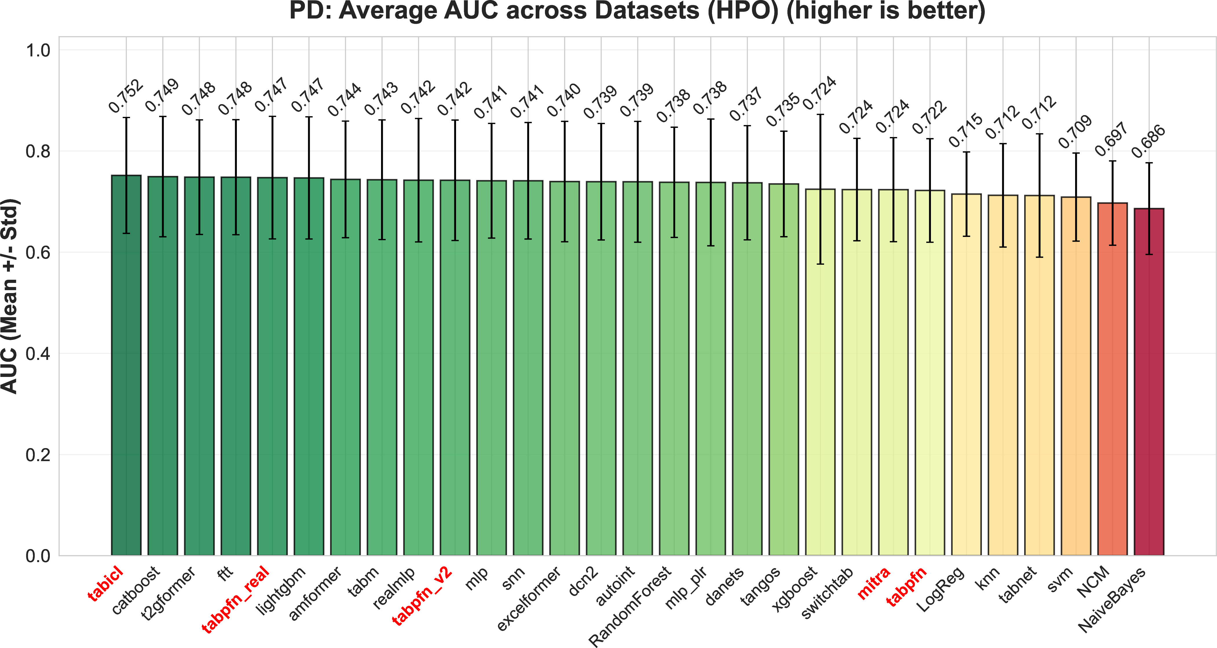
A second observation from Figure 2 concerns the small magnitude of performance differences for a set of well-performing learning algorithms, including GBM-type approaches, PFNs, and Random Forests. We observe a similar trend for other metrics of classification performance, as reported in Table 4.
A third observation concerns the performance differences among TFMs. Whereas TabICL is best in class, TabPFN-Real also ranks among the stronger methods. TabPFNv2 performs in the middle of the distribution, while MITRA and TabPFN rank among the weaker TFMs for default prediction.
Table 4 summarizes the full set of metrics utilized in the PD classification benchmark.
| Method | Discrimination | Calibration | Classification (threshold-based) | |||||||||
|---|---|---|---|---|---|---|---|---|---|---|---|---|
| 2-5(lr)6-7(lr)8-13 | AUC | Gini | KS | AP | Brier \(\downarrow\) | LogLoss \(\downarrow\) | Acc | Bal-Acc | F1 | Precision | Recall | MCC |
| Foundation models | ||||||||||||
| TabICL | 0.7517 | 0.5035 | 0.3987 | 0.4933 | 0.1619 | 0.5081 | 0.7125 | 0.6734 | 0.5047 | 0.4368 | 0.6547 | 0.3265 |
| TabPFNv2 | 0.7421 | 0.4843 | 0.3867 | 0.4891 | 0.1320 | 0.4119 | 0.6970 | 0.6685 | 0.5025 | 0.4364 | 0.6666 | 0.3201 |
| TabPFN-Real | 0.7474 | 0.4948 | 0.3972 | 0.4949 | 0.1612 | 0.5067 | 0.6975 | 0.6732 | 0.5092 | 0.4426 | 0.6744 | 0.3296 |
| MITRA | 0.7236 | 0.4471 | 0.3466 | 0.4563 | 0.1391 | 0.4329 | 0.6449 | 0.6449 | 0.4702 | 0.3944 | 0.6801 | 0.2729 |
| TabPFN | 0.7220 | 0.4440 | 0.3433 | 0.4498 | 0.1407 | 0.4378 | 0.6778 | 0.6491 | 0.4716 | 0.3926 | 0.6510 | 0.2758 |
| Gradient boosting | ||||||||||||
| CatBoost | 0.7494 | 0.4988 | 0.3982 | 0.4923 | 0.1331 | 0.4146 | 0.7129 | 0.6746 | 0.5074 | 0.4425 | 0.6540 | 0.3288 |
| LightGBM | 0.7468 | 0.4936 | 0.3956 | 0.4918 | 0.1318 | 0.4187 | 0.6919 | 0.6714 | 0.5064 | 0.4351 | 0.6826 | 0.3216 |
| XGBoost | 0.7244 | 0.4489 | 0.3595 | 0.4781 | 0.1343 | 0.4319 | 0.6416 | 0.6597 | 0.5010 | 0.4311 | 0.7230 | 0.3051 |
| Classical ML | ||||||||||||
| Logistic Reg. | 0.7148 | 0.4296 | 0.3330 | 0.4294 | 0.1428 | 0.4432 | 0.6700 | 0.6429 | 0.4599 | 0.3760 | 0.6475 | 0.2609 |
| Random Forest | 0.7381 | 0.4763 | 0.3726 | 0.4765 | 0.1358 | 0.4226 | 0.6895 | 0.6588 | 0.4868 | 0.4160 | 0.6567 | 0.2976 |
| Naive Bayes | 0.6861 | 0.3723 | 0.2956 | 0.3974 | 0.3069 | 2.2809 | 0.6124 | 0.6173 | 0.4317 | 0.3387 | 0.6768 | 0.2124 |
| KNN | 0.7124 | 0.4248 | 0.3370 | 0.4438 | 0.1385 | 0.5808 | 0.6573 | 0.6462 | 0.4753 | 0.3948 | 0.6825 | 0.2749 |
| SVM | 0.7089 | 0.4178 | 0.3268 | 0.4239 | 0.1434 | 0.4453 | 0.6601 | 0.6387 | 0.4557 | 0.3712 | 0.6508 | 0.2530 |
| NCM | 0.6971 | 0.3941 | 0.3111 | 0.4094 | 0.2186 | 0.6258 | 0.6471 | 0.6321 | 0.4498 | 0.3620 | 0.6618 | 0.2390 |
| Deep learning | ||||||||||||
| MLP | 0.7412 | 0.4824 | 0.3829 | 0.4816 | 0.1332 | 0.4402 | 0.6928 | 0.6682 | 0.5002 | 0.4334 | 0.6686 | 0.3191 |
| MLP-PLR | 0.7379 | 0.4758 | 0.3844 | 0.4865 | 0.1344 | 0.4688 | 0.6971 | 0.6679 | 0.4995 | 0.4347 | 0.6553 | 0.3181 |
| SNN | 0.7411 | 0.4823 | 0.3829 | 0.4817 | 0.1370 | 0.4550 | 0.7072 | 0.6675 | 0.4970 | 0.4320 | 0.6427 | 0.3154 |
| RealMLP | 0.7423 | 0.4846 | 0.3869 | 0.4884 | 0.1656 | 0.5167 | 0.7085 | 0.6708 | 0.5033 | 0.4461 | 0.6490 | 0.3259 |
| TabNet | 0.7120 | 0.4241 | 0.3363 | 0.4483 | 0.1392 | 0.4342 | 0.6617 | 0.6431 | 0.4728 | 0.4057 | 0.6544 | 0.2716 |
| SwitchTab | 0.7238 | 0.4476 | 0.3501 | 0.4540 | 0.1390 | 0.4324 | 0.6799 | 0.6532 | 0.4772 | 0.4035 | 0.6561 | 0.2862 |
| FTT | 0.7482 | 0.4964 | 0.3942 | 0.4895 | 0.1314 | 0.4129 | 0.7000 | 0.6734 | 0.5041 | 0.4342 | 0.6701 | 0.3248 |
| T2G-Former | 0.7483 | 0.4965 | 0.3930 | 0.4894 | 0.1318 | 0.4159 | 0.7073 | 0.6737 | 0.5056 | 0.4375 | 0.6615 | 0.3274 |
| DCN2 | 0.7393 | 0.4786 | 0.3814 | 0.4775 | 0.1338 | 0.4425 | 0.6963 | 0.6673 | 0.4996 | 0.4308 | 0.6641 | 0.3149 |
| ExcelFormer | 0.7396 | 0.4792 | 0.3809 | 0.4813 | 0.1333 | 0.4162 | 0.6945 | 0.6646 | 0.4960 | 0.4294 | 0.6578 | 0.3114 |
| AutoInt | 0.7391 | 0.4782 | 0.3791 | 0.4816 | 0.3200 | 5.3695 | 0.8112 | 0.6092 | 0.3228 | 0.5500 | 0.2715 | 0.2723 |
| DANets | 0.7372 | 0.4745 | 0.3739 | 0.4778 | 0.1354 | 0.4428 | 0.6921 | 0.6648 | 0.4935 | 0.4328 | 0.6557 | 0.3127 |
| TANGOS | 0.7349 | 0.4697 | 0.3681 | 0.4737 | 0.1362 | 0.4389 | 0.6847 | 0.6602 | 0.4863 | 0.4184 | 0.6611 | 0.3024 |
| AMFormer | 0.7439 | 0.4877 | 0.3879 | 0.4885 | 0.1330 | 0.4243 | 0.7063 | 0.6706 | 0.4992 | 0.4359 | 0.6510 | 0.3206 |
5.2 LGD modeling↩︎
Next, we examine the performance of TFMs for LGD prediction. Figure 3 reports the corresponding results in terms of the average \(R^2\) measure across datasets. Results for (R)MSE and MAE are similar and reported in Table 5.
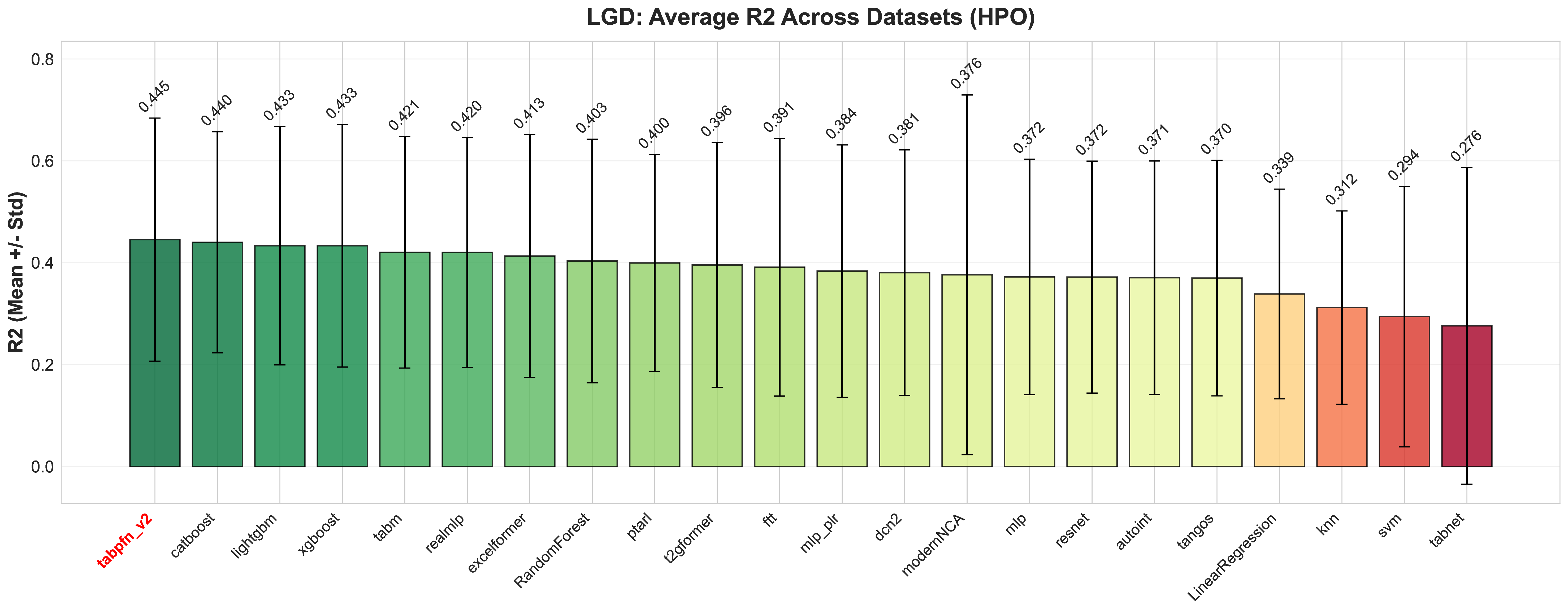
A first observation from Figure 3 is that, as for PD modeling, the best performance is, on average, achieved by a TFM, i.e., TabPFNv2. LGD modeling is a challenging task, which prior work often associates with the peculiar shape of the loss distributions, as observed in Figure 1. Therefore, it is notable to find that also for LGD prediction, despite the challenge involved in this task, TFMs outperform the state-of-the-art methods in the field. This confirms the occurrence of a paradigm shift, both for classification and regression, as highlighted in the previous section.
TabPFNv2 supports regression by discretizing the continuous target into a piecewise-constant probability distribution and training the model to predict this distribution, effectively framing regression as an ordinal classification problem. This approach can be considered conceptually suitable for LGD distributions, as it provides the required flexibility to fit widely varying and non-normal distributions, and is confirmed by our experiments to perform well on the LGD data employed here.
A second observation is that, as for PD estimation, several methods are close in average performance, although more variability is observed compared to the PD results.
A third observation is that our experiments confirm the strong performance of boosting ensemble methods, across PD and LGD modeling tasks, as reported in the literature.
The full set of metrics utilized in the LGD regression benchmark is summarized in Table 5.
| Method | Error / Fit | Correlation & Variance | |||||||
|---|---|---|---|---|---|---|---|---|---|
| 2-7(lr)8-10 | \(R^2\) | MSE \(\downarrow\) | RMSE \(\downarrow\) | MAE \(\downarrow\) | MedAE \(\downarrow\) | MaxErr \(\downarrow\) | Pearson | Spearman | Expl. Var |
| Foundation model | |||||||||
| TabPFNv2 | 0.4455 | 0.0704 | 0.2522 | 0.1889 | 0.1410 | 0.8890 | 0.6596 | 0.6094 | 0.4586 |
| Gradient boosting | |||||||||
| CatBoost | 0.4401 | 0.0702 | 0.2540 | 0.1885 | 0.1369 | 0.9052 | 0.6499 | 0.6023 | 0.4435 |
| LightGBM | 0.4334 | 0.0706 | 0.2545 | 0.1879 | 0.1376 | 0.9076 | 0.6434 | 0.5969 | 0.4407 |
| XGBoost | 0.4334 | 0.0704 | 0.2540 | 0.1911 | 0.1442 | 0.8998 | 0.6393 | 0.5982 | 0.4380 |
| Classical ML | |||||||||
| Linear Reg. | 0.3387 | 0.0832 | 0.2777 | 0.2139 | 0.1725 | 0.9366 | 0.5673 | 0.5359 | 0.3410 |
| Random Forest | 0.4035 | 0.0748 | 0.2619 | 0.1962 | 0.1423 | 0.8925 | 0.6178 | 0.5710 | 0.4100 |
| KNN | 0.3120 | 0.0839 | 0.2815 | 0.2216 | 0.1778 | 0.8488 | 0.5583 | 0.5145 | 0.3185 |
| SVM | 0.2942 | 0.0885 | 0.2856 | 0.2117 | 0.1515 | 0.9238 | 0.5548 | 0.5302 | 0.3187 |
| Deep learning | |||||||||
| MLP | 0.3722 | 0.0798 | 0.2700 | 0.1898 | 0.1200 | 0.9261 | 0.6096 | 0.5704 | 0.3814 |
| MLP-PLR | 0.3836 | 0.0782 | 0.2669 | 0.1787 | 0.1030 | 0.9365 | 0.6231 | 0.5806 | 0.3999 |
| RealMLP | 0.4203 | 0.0730 | 0.2588 | 0.1844 | 0.1268 | 0.9212 | 0.6369 | 0.5958 | 0.4261 |
| TabM | 0.4206 | 0.0727 | 0.2581 | 0.1852 | 0.1290 | 0.9265 | 0.6384 | 0.5914 | 0.4255 |
| TabNet | 0.2763 | 0.0942 | 0.2902 | 0.2278 | 0.1772 | 0.9363 | 0.4799 | 0.4543 | 0.2839 |
| FTT | 0.3912 | 0.0774 | 0.2649 | 0.1801 | 0.1068 | 0.9362 | 0.6314 | 0.5907 | 0.4057 |
| T2G-Former | 0.3957 | 0.0768 | 0.2644 | 0.1811 | 0.1089 | 0.9419 | 0.6354 | 0.5876 | 0.4106 |
| DCN2 | 0.3805 | 0.0793 | 0.2685 | 0.1945 | 0.1409 | 0.9388 | 0.6049 | 0.5657 | 0.3861 |
| AutoInt | 0.3706 | 0.0800 | 0.2701 | 0.1909 | 0.1234 | 0.9326 | 0.6105 | 0.5679 | 0.3882 |
| ExcelFormer | 0.4132 | 0.0739 | 0.2597 | 0.1843 | 0.1270 | 0.9361 | 0.6234 | 0.5780 | 0.4212 |
| ResNet | 0.3719 | 0.0800 | 0.2704 | 0.1917 | 0.1270 | 0.9414 | 0.6095 | 0.5617 | 0.3807 |
| TANGOS | 0.3699 | 0.0798 | 0.2705 | 0.1898 | 0.1195 | 0.9288 | 0.6047 | 0.5652 | 0.3810 |
| Specialised / other | |||||||||
| ModernNCA | 0.3763 | 0.0789 | 0.2616 | 0.1718 | 0.0968 | 0.9356 | 0.6202 | 0.5884 | 0.3904 |
| PTARL | 0.3997 | 0.0763 | 0.2645 | 0.1986 | 0.1497 | 0.9070 | 0.6193 | 0.5808 | 0.4027 |
5.3 Statistical analysis of PFN performance↩︎
To contextualize performance differences across learners and datasets, we employ three complementary statistical analyses, following standard practice in the benchmarking literature [5], [6], [102]. We begin with the PAMA analysis to identify learners that achieve top performance most frequently, then use the Friedman test to formally establish whether performance differences are globally non-random, and finally use pairwise Wilcoxon signed-rank tests with Win/Loss ratios to probe the magnitude and significance of the pairwise differences. All analyses are based on the AUC for PD models and \(R^2\) for LGD models.
A natural first question that emerges is the following: across all datasets, which learner most often yields the best performance? The Probability of Achieving Maximal Accuracy (PAMA) analysis [104] provides an answer to this question by computing, across all learners, the fraction of fold-level observations in which a learner achieves the highest score. This provides an intuitive, rank-based summary of competitiveness that is robust to outlying datasets and does not require us to make any assumptions about the distribution of performance differences.
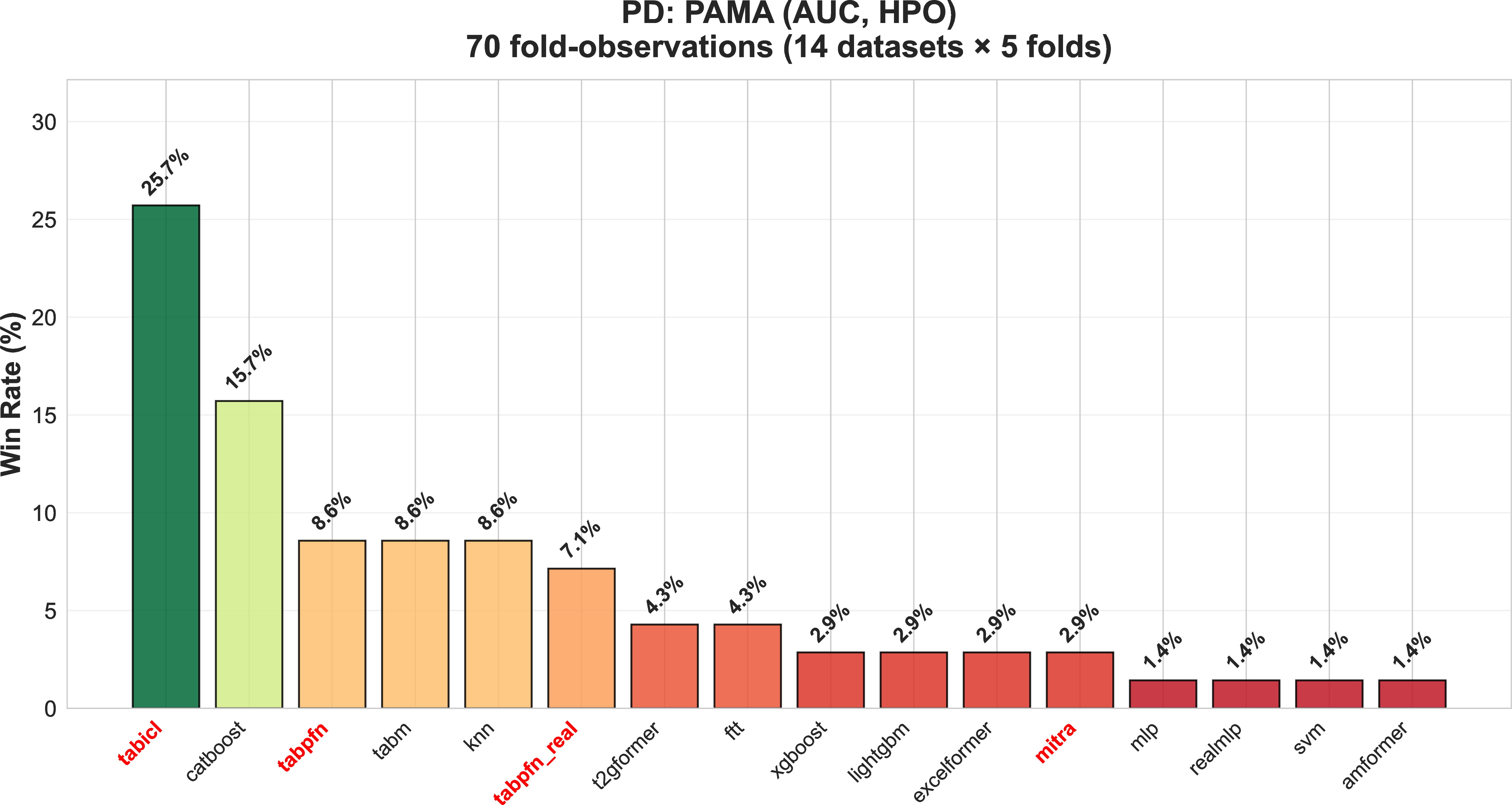
Figures 4 and 5 show the PAMA results for the PD and LGD benchmarks, respectively. For PD, the performance of TabICL stands out. It achieves the highest AUC in \(25.7\%\) of fold-level observations (18 out of 70), followed by CatBoost at \(15.7\%\). Notably, foundation models as a group achieve the best performance in \(44.3\%\) of all folds, indicating their collective competitiveness, even when no single model dominates. For LGD regression, TabPFNv2 is the only foundation model included. It achieves the highest \(R^2\) in \(45.7\%\) of folds (16 out of 35), placing it well ahead of all competitors on this benchmark too.
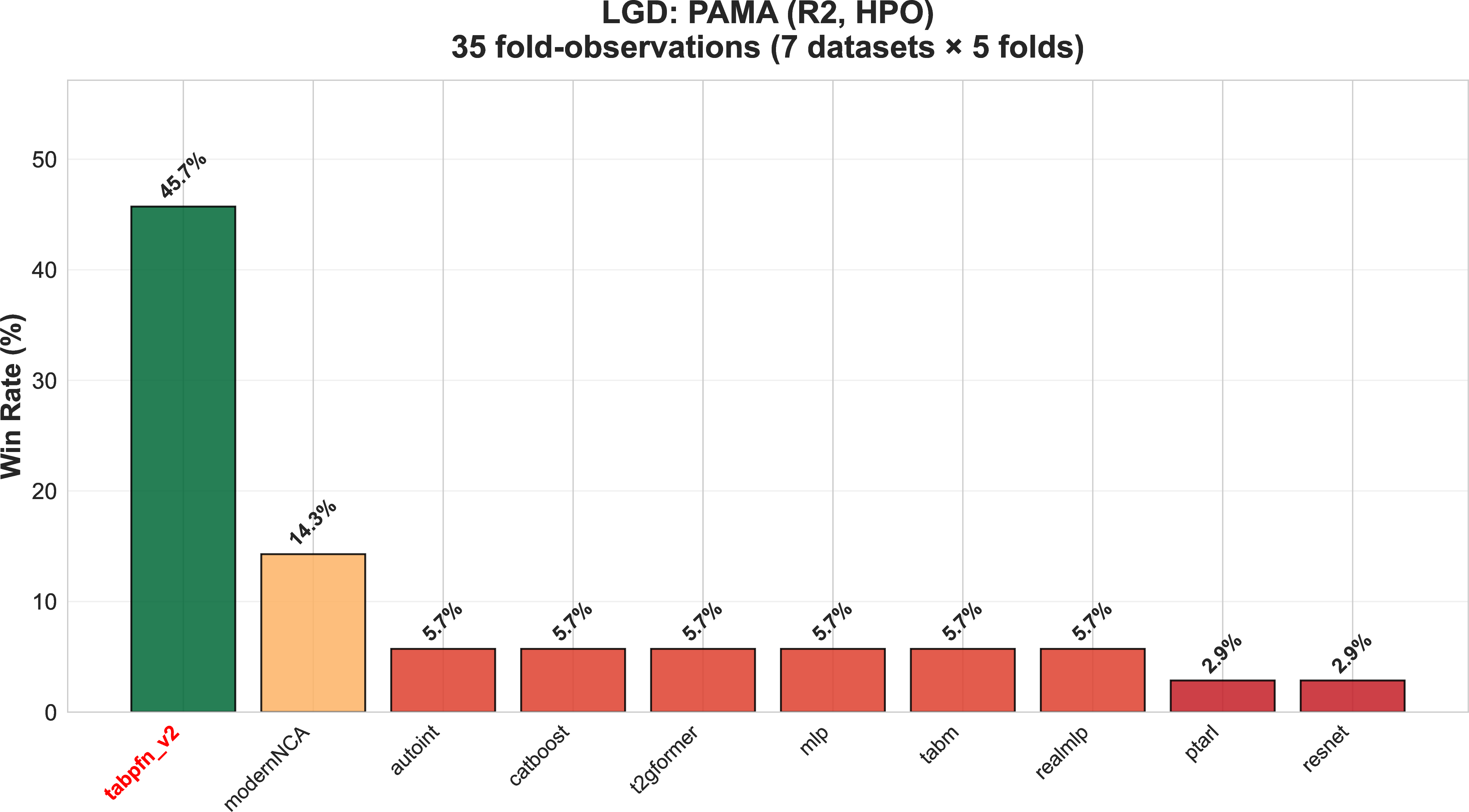
The PAMA analysis is descriptive and does not assess whether observed performance differences could have arisen by chance. To establish this formally, we apply the Friedman test with Iman–Davenport correction [102], [105], [106], a non-parametric test that assesses whether the overall ranking of learners across datasets deviates significantly from what would be expected under the null hypothesis that all methods perform equally. For the PD benchmark (\(N = 14\) datasets, \(k = 29\) methods), \(F_F = 7.01\) (\(p = 1.11 \times 10^{-16}\)); for the LGD benchmark (\(N = 7\) datasets, \(k = 22\) methods), \(F_F = 3.84\) (\(p = 1.12 \times 10^{-6}\)). Both tests strongly reject the null hypothesis, confirming that the performance differences observed in the PAMA analysis are not attributable to chance and that post-hoc pairwise comparisons are warranted.
Having established that global differences are statistically significant, we turn to pairwise comparisons to identify which specific pairs of learners differ statistically significantly in terms of performance. For each pair, we test the null hypothesis that the median performance difference is zero using the Wilcoxon signed-rank test [103], which accounts for both the direction and magnitude of differences across datasets. \(p\)-values are adjusted for multiple comparisons using Holm’s step-down method [107], [108], applied over all 406 PD and 231 LGD pairs, respectively. Figures 6 and 7 display the results where cell text reports the Win/Loss (W/L) ratio, and a trailing asterisk (*) marks pairs with a statistically significant difference (\(p \leq 0.05\), Holm-corrected).
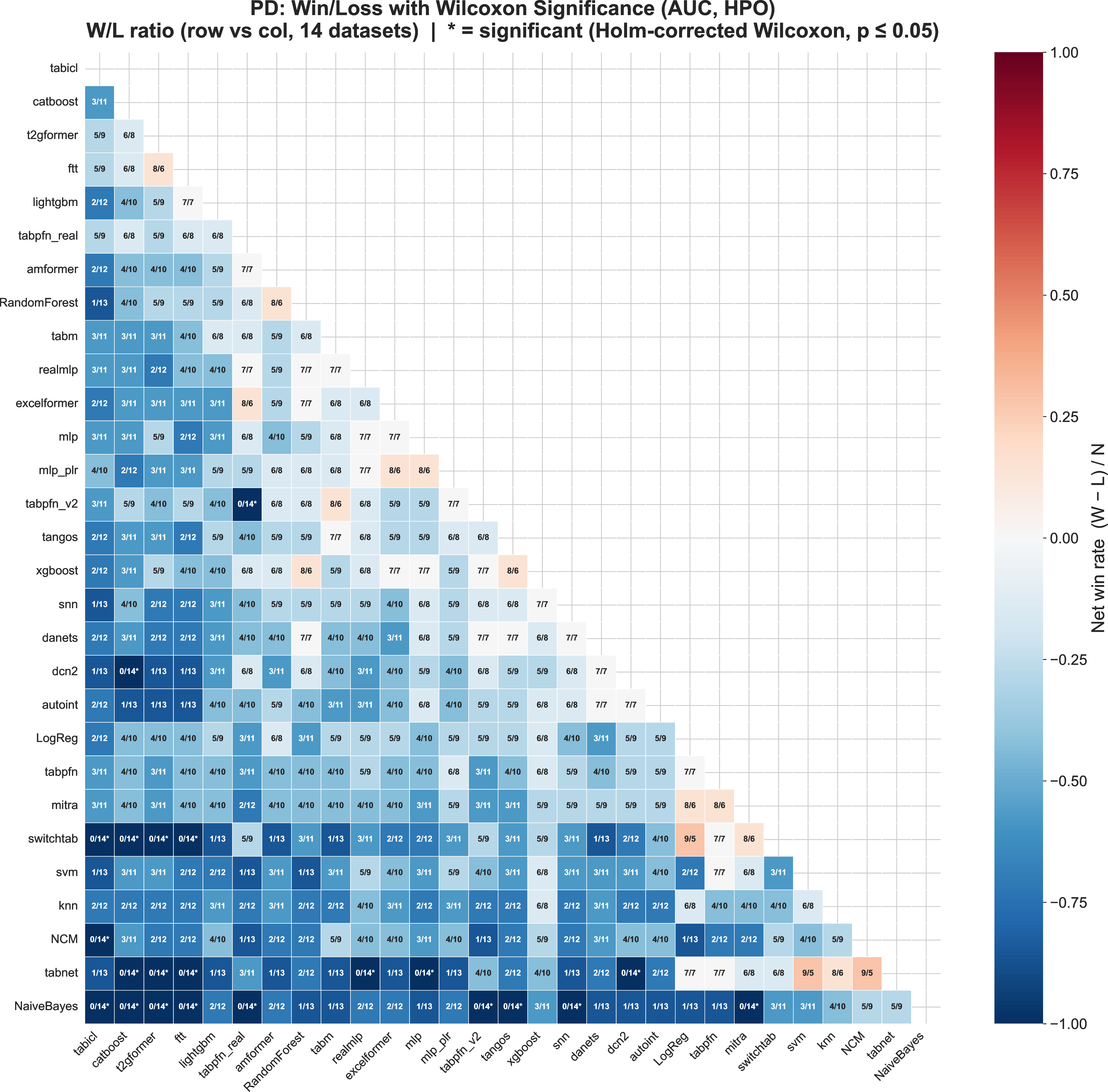
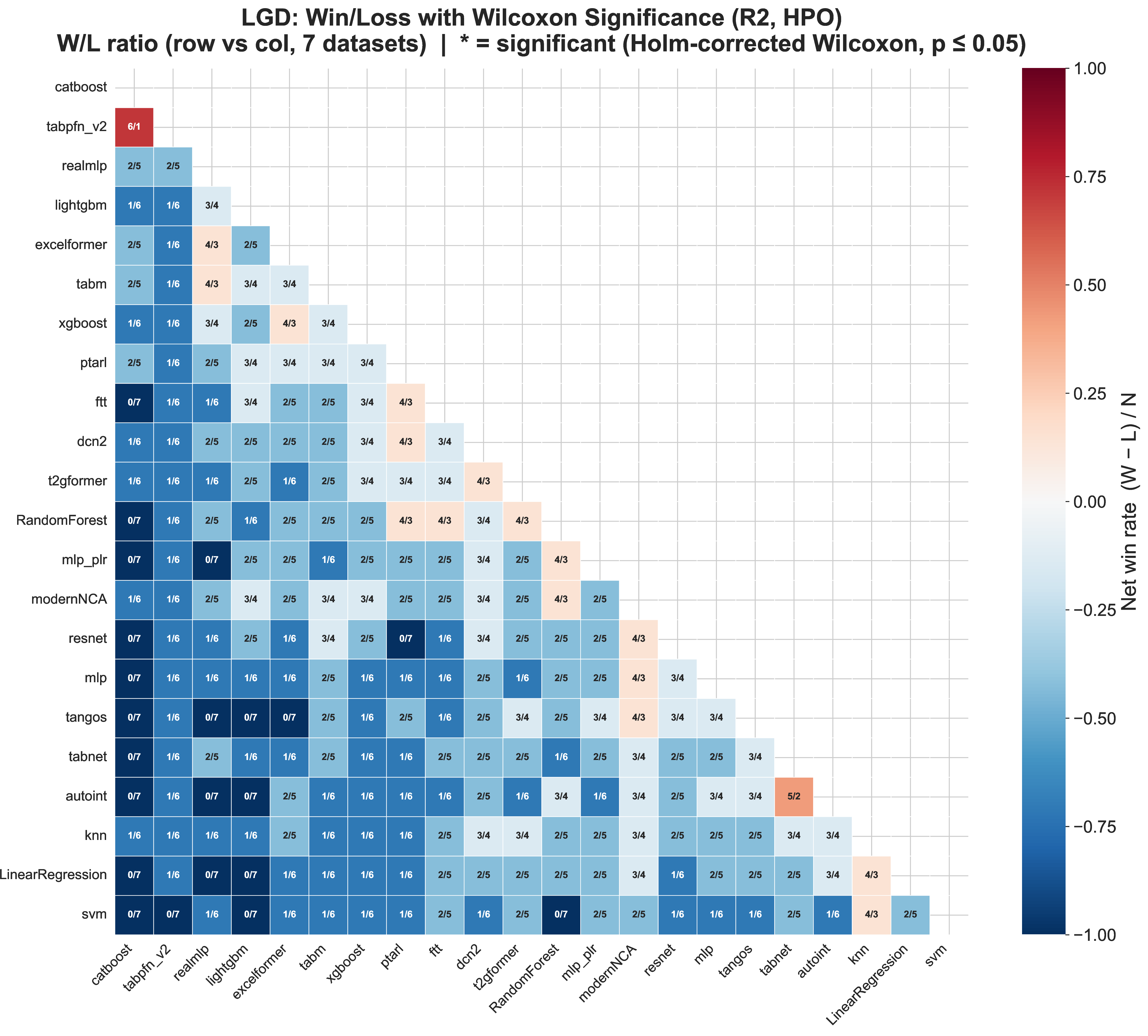
For the PD benchmark, 22 out of 406 pairwise comparisons are statistically significant after Holm correction. For LGD, none of the 231 pairwise comparisons reach significance. The limited number of significant pairwise differences is not surprising and reflects two structural features of the benchmarking setup. First, the number of datasets constrains statistical power: the Wilcoxon signed-rank test requires sufficient paired observations to reliably detect non-zero median differences, and with \(N = 14\) PD datasets and only \(N = 7\) LGD datasets, this power is inherently limited. For LGD in particular, the minimum achievable two-sided \(p\)-value for a single comparison is \(2/2^7 \approx 0.016\), and after Holm correction for 231 simultaneous tests, this threshold rises substantially, making it virtually impossible to find a difference in performance between any individual pair to be statistically significant. Second, the relatively small magnitude of performance differences among the top methods — which can be clearly observed in Figures 2 and 3 — means that even where directional evidence is consistent, differences may not be large enough to cross the significance threshold after multiple-comparison correction. These results, therefore, do not contradict the omnibus Friedman test, which has substantially greater power to detect global heterogeneity than individual pairwise tests have to localize it.
Taken together, the three analyses paint a consistent and favorable picture for TFMs. The PAMA analysis shows that foundation models collectively achieve the highest performance in \(44.3\%\) of PD folds, with TabICL leading individually, and that TabPFNv2 alone wins \(45.7\%\) of LGD folds. The Friedman test confirms that these differences in method rankings are not attributable to chance. Overall, these results provide consistent support for the conclusion that TFMs are competitive challengers to established methods in credit risk prediction.
5.4 Dataset size↩︎
A particular feature of TFMs that may be appealing towards credit risk modeling is their potential use for small portfolios, resulting in small datasets.
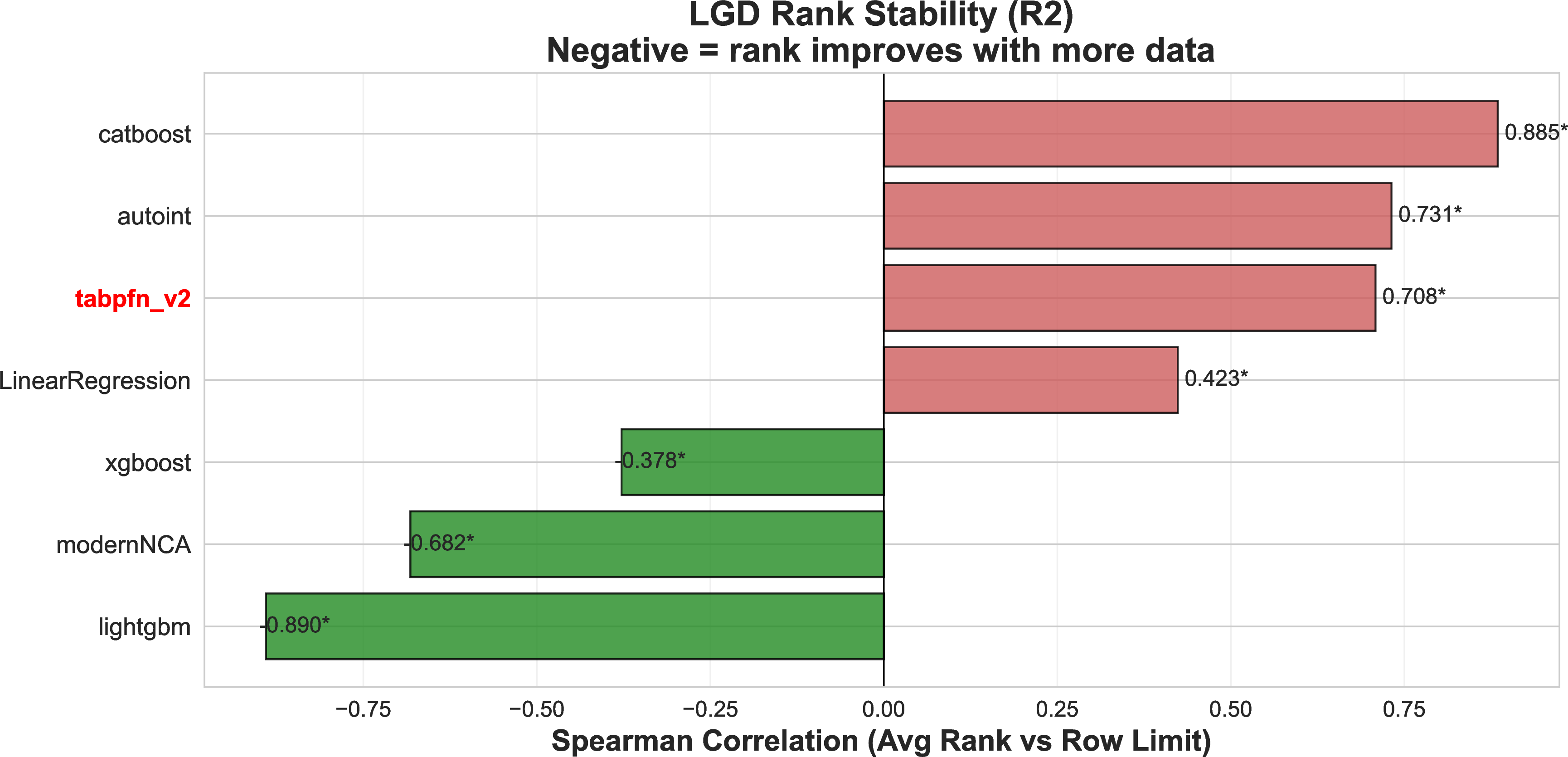
To assess the ability of TFMs for handling small datasets, we next analyze the relation between learner performance, more specifically, the rank of a given method, and dataset size (in number of observations) using Spearman’s rank correlation coefficient. Figures 8 and 9 report the corresponding results for PD and LGD modeling, respectively. The positive correlation observed for TFMs indicates that they rank higher (i.e., show relatively worse performance compared to other methods) on larger datasets. In other words, for smaller datasets, TFMs perform relatively better. We observe this tendency for PD and LGD modeling, supporting our hypothesis that TFMs are particularly appealing for small portfolios, and, more generally, small data settings.
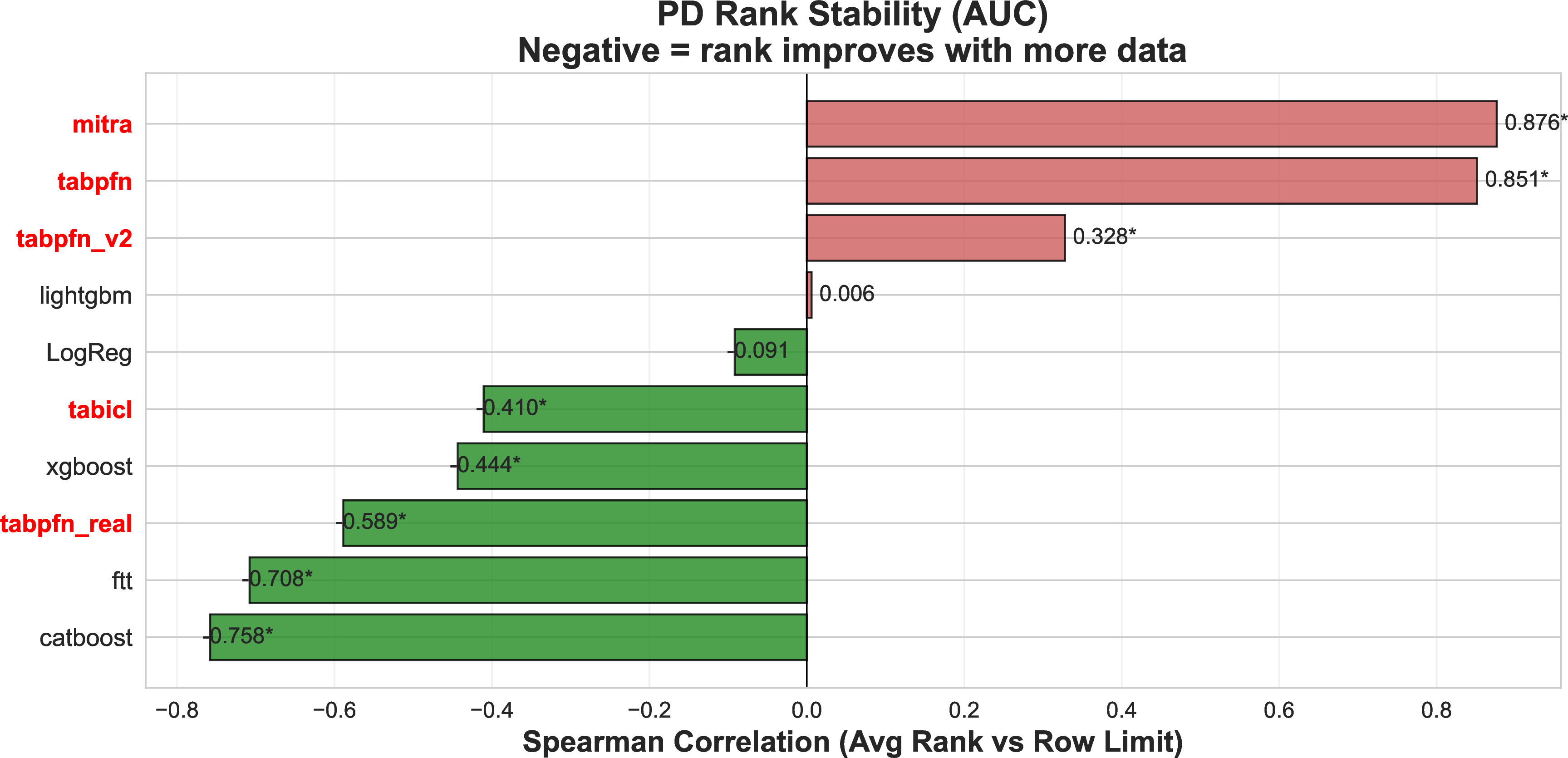
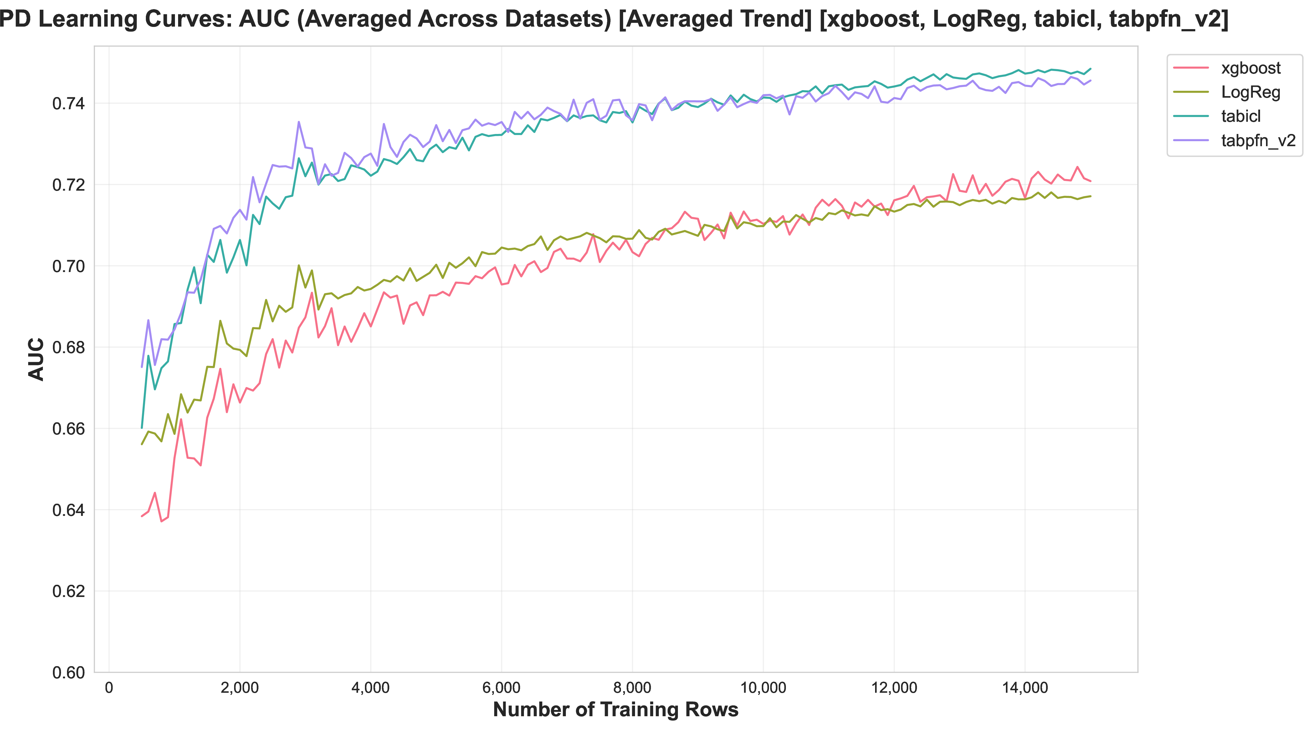
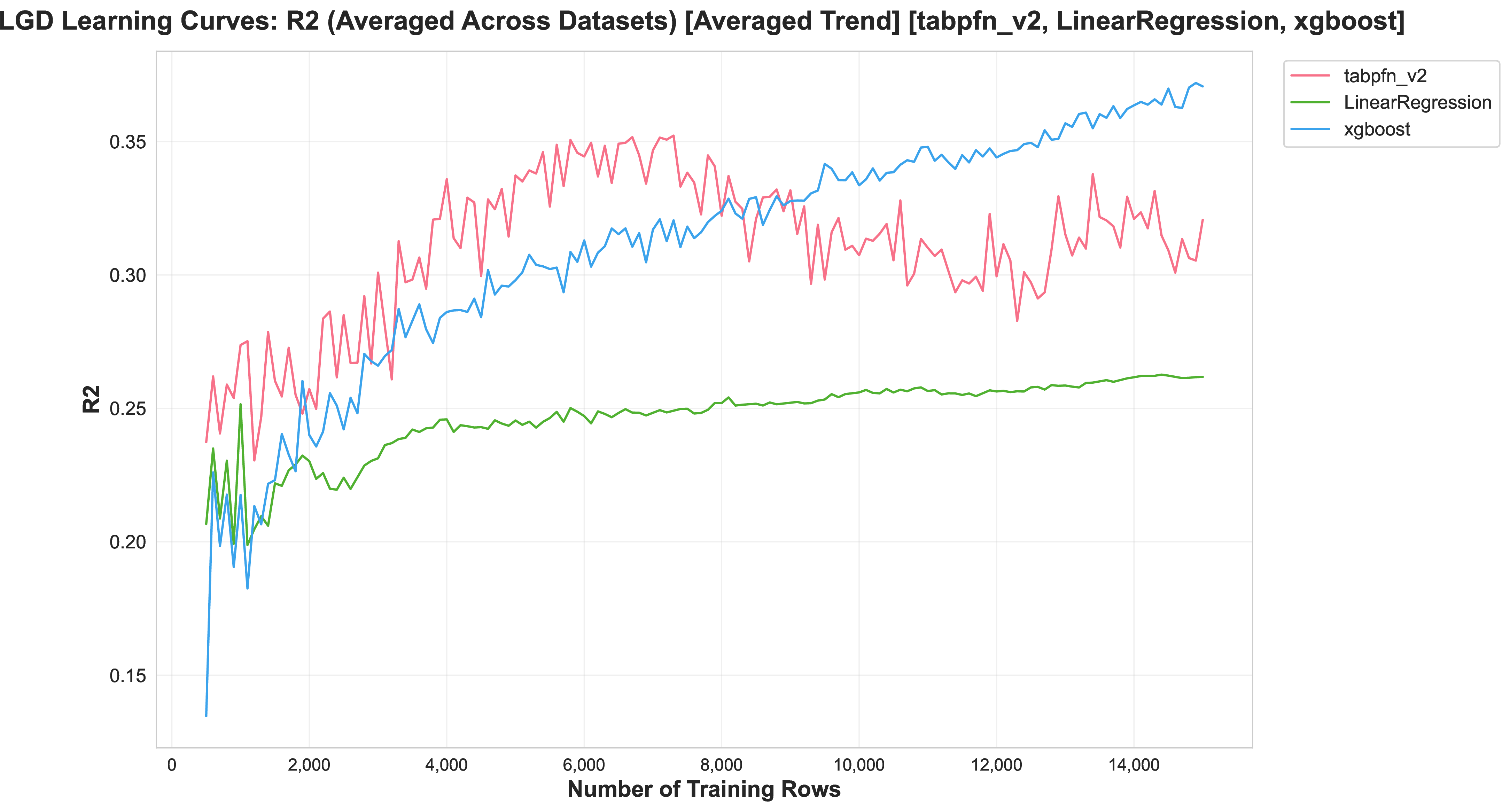
A second experiment to assess the impact of dataset size on the performance of TFMs evaluates the evolution of average performance as the number of randomly sampled observations increases (from 500 to 15,000) for datasets that include more than 15,000 observations. Figures 10 and 11 report the results for PD and LGD modeling, respectively, and include the so-called learning curves for the TFMs and a selected set of baseline methods, i.e., Logistic Regression, CatBoost, FTT, LightGBM, and XGBoost. A general—unsurprising—tendency is that performance increases with dataset size across methods. The performance of TFMs is substantially above the performance of the baseline methods for smaller numbers of observations, and the difference in performance decreases as the size of the dataset increases. For LGD modeling, similar results are found, as shown in Figure 11. Whereas the baseline method, XGBoost, performs substantially worse than TabPFNv2 for small dataset sizes, it eventually overtakes TabPFNv2 when dataset sizes exceed 8,000 observations. It is unclear why TabPFNv2’s performance declines at this point. Further research may focus on confirming and explaining this behavior.
6 Conclusions↩︎
This paper provides an extensive empirical evaluation of TFMs for credit risk prediction, benchmarking them against a broad panel of classical, tree-based, and deep learning methods across 14 PD and 7 LGD datasets. The results consistently favor foundation models. For PD classification, TabICL achieves the highest average rank and leads the PAMA analysis with the highest AUC in \(25.7\%\) of fold-level observations, while foundation models as a group attain top performance in \(44.3\%\) of all folds. For LGD regression, TabPFNv2, the only foundation model evaluated, achieves the highest \(R^2\) in \(45.7\%\) of folds, placing it ahead of all tuned competitors, including GBMs. Statistical analysis via the Friedman test confirms that these differences in learner rankings are not attributable to chance, and Win/Loss comparisons show that top-ranked methods, including foundation models, significantly outperform weaker baselines.
A noteworthy finding concerns the relationship between dataset size and relative performance. TFMs show a consistent advantage on smaller datasets, with their relative performance deteriorating as dataset size grows. This finding directly supports the use case motivating much of the interest in foundation models for credit risk: small-data settings such as SME lending, low-default portfolios, and specialized corporate segments where conventional methods struggle due to limited training signals. The learning curve analysis confirms this pattern, showing that TabPFNv2 leads clearly at small sample sizes before tuned GBMs gradually close the gap as data availability increases.
From a practical perspective, PFNs offer several advantages. They eliminate the need for task-specific hyperparameter tuning and retraining, improving time-to-model and reducing operational costs. Their generality supports consistent modeling across risk parameters, which can simplify governance and may ease supervisory review. Potential benefits from a customer perspective include more stable, consistent decisions across portfolios and institutions and, with appropriate safeguards, opportunities to reduce historical biases by leveraging priors learned from broad synthetic data. Importantly, PFNs can also complement established risk modeling practices, facilitating risk prediction in early stages of the product lifecycle where available data is very limited. A later migration to, for example, a logit- or GBM-based score once a sufficient amount of (repayment) data has been gathered is straightforward, potentially reducing dependency on external credit rating agencies for new product scoring.
Important avenues for future work remain. We plan to include established LGD econometric baselines (e.g., beta regression and two-part models), and evaluate profit-based measures such as EMPC more broadly. We also aim to analyze PFN behavior under specific credit risk challenges, including low-default portfolios, reject inference framed as missing data, distribution shifts, and fairness constraints. Finally, interpretability remains essential: we will compare feature attributions derived from PFN and GBM pipelines using SHAP and alternatives such as XPER [68].