Abstract
This paper considers games where the utilities for agents are the sum of a term proportional to a social utility, and another term that is an individual cost or reward. The agents are assumed to be irrational in their perception of the individual cost or reward. The multi equilibrium game is regularized, and its strictly concave potential function is used to select a unique equilibrium. This selected equilibrium is shown to be an \(\epsilon-\)equilibrium of the original game, where \(\epsilon\) is parametrized by the regularizing function. A minorization-maximization based iterative learning scheme is proposed to learn equilibria in this game. This scheme converges to the potential-optimal equilibrium, and has superior convergence behaviour in comparison to gradient and best response methods.
1 Introduction↩︎
In many games and optimization problems, an agent’s payoff combines an individual cost with a reward proportional to a collective social utility. This captures scenarios where agents independently pursue a shared objective, making success dependent on coordination. Such interactions naturally form coordination games [1] and, in some cases, aggregative games, where each agent responds to an aggregate of others’ actions [2]. Under mild conditions, they admit a (weighted) potential game structure, enabling equilibrium analysis via a global function [3]. Examples for scenarios where such problems arise, include energy markets, where electricity consumers utilize a shared resource while collectively aiming to meet a common carbon emission target [4], and the multi agent exploration problem [5], where multiple agents try to reach a common target or destination, while moving in a coordinated but distributed fashion. A particular example of multi agent exploration is the rendezvous problem [6], in which multiple robots, initially distributed across an unknown or unexplored environment, seek to reach a common destination while incurring individual energy costs. In all these cases, performance ultimately depends on the agents’ ability to coordinate through the effects of their collective actions.
While not all potential games correspond to meaningful social utilities, the closely related class of social purpose games [7] explicitly decomposes utilities into a collective-benefit term and an individual cost, capturing a broad range of problems involving common or public resources.
From another perspective, the presence of a collective objective connects this framework to cooperative game theory [8], where one studies how groups of agents generate and share value. In particular, when the underlying social utility exhibits supermodularity, one can leverage strong structural properties—such as increasing returns—to obtain existence, monotonicity, and robustness guarantees for equilibria (see, e.g., [9]). Finally, in the large-population regime, when the impact of any single agent on the aggregate becomes negligible, the model relates to mean-field games [10]. This approximation is attractive for analyzing asymptotic system behavior, but comes at a cost: by averaging interactions, it tends to wash out individual heterogeneity and may fail to capture nuanced agent preferences or cost perceptions.
In this paper, we consider such an additive utility model. However, we assume that agents are not fully rational in their perception of individual costs. When agents are human, this deviation from rationality may arise from behavioral biases [11]. For non-human agents, bounded rationality may instead stem from limitations in information, perspective, or computational capacity, which can hinder effective coordination. Several modeling paradigms have been proposed to capture such deviations from perfect rationality. Quantal best-response [12] and noisy discrete choice models [13] introduce stochasticity in decision-making, typically assuming that agents respond smoothly to payoff differences (e.g., via logit dynamics). These models are analytically tractable and well-suited for equilibrium learning, but they primarily capture random errors rather than systematic biases in perception. Distributionally robust game [14] formulations, on the other hand, account for ambiguity in agents’ beliefs by considering worst-case distributions over uncertainties. While they provide strong robustness guarantees, they tend to reflect ambiguity aversion at the population level rather than individual-level cognitive distortions, and may lead to overly conservative behaviors.
In contrast, we adopt prospect theory (PT) [15], which explicitly models systematic deviations from expected utility maximization by incorporating reference dependence, loss aversion, and probability distortion. Prospect theory addresses well-documented shortcomings of classical von Neumann–Morgenstern expected utility theory (EUT) [16], whose assumption of fully rational agents is often contradicted by experimental evidence [11]. A variety of prospect-theoretic models exist [17], differing in how they model value functions and probability weighting, and often tailored to specific applications.
Many games, including those with prospect-theoretic utilities [18], admit multiple equilibria, complicating both analysis and learning. To address this, we introduce a regularized (perturbed) game, adding a small term to the utility or potential function. The rgularized potential function has a unique maximum, which selects a unique equilibrium while preserving the structure of the original game. This is analogous to regularization in machine learning to ensure unique maximizers. The regularizer thus acts as a weak equilibrium selection mechanism, linking the perturbed equilibrium to the original set of equilibria. Learning this single equilibrium is the next question of interest. The kind of algorithm that can be used for learning is intricately tied to the structure of the game. Monotone games and potential games show convergence under gradient type learning dynamics [19]. In the case of aggregative games, best response learning converges under strong assumptions on the structure of the interaction between the users’ strategies and utilities [20]. However, the performance of many learning algorithms worsens when the game is non smooth, i.e., the utilities are no longer continuously differentiable. To address this challenge, we propose a minorization–maximization (MM) [21] based learning scheme. The key idea is to replace the original optimization problem with a sequence of surrogate problems whose optima converge to a chosen equilibrium. The required aggregate information is communicated through a coordinating agent, enabling scalable learning despite the presence of non-standard utility functions. We see that MM improves convergence speed while leveraging the game’s potential structure. Since it can be used to learn equilibria in games with smooth and non-smooth utilities, we see that it presents itself as an algorithm which can be used across a variety of applications ranging from electricity markets to multi agent coordination.
Utilities reflecting PT preferences encode sensitive information (e.g., risk attitudes, reference points). Our framework requires only aggregate information, protecting individual preferences. The surrogate optimization in MM further supports privacy-preserving modifications, such as adding noise or using secure aggregation, without compromising convergence to the perturbed equilibrium.
1.1 Literature Review↩︎
Potential games [3] are a well studied class of games with enough structure to allow convergence under different types of learning. Results for existence of equilibria and convergence of leaning schemes for finite games and games with differentiable utilities are found in [22]. Convergence results for best and better response dynamics in near potential games, for games with finite strategy sets and mixed strategies, are provided in [23].
Social purpose games [7] are a subset of the class of games we study, since they additionally have the aggregative property. Moreover [7] focuses on the emergence of cooperation in such games, whereas in this paper we focus on agent irrationality and learning to reach a specific equilibrium.
Prospect theory has been used in economics for many decades, in order to model decision making under uncertainty [24]. Some works that use PT models in finite games include [25],[26],[27] and [28]. These works provide results for existence of Nash equilibria. In [29], a piecewise linear PT transformation is considered, and results are obtained for existence of equilibria. A broad survey of different papers that have used prospect theory in modelling economics of power systems is presented in [30]. In [31] existence results for local Nash equilibria are obtained under non smooth PT transformations. In [18], the effect of PT transforms on the set of equilibria is characterized analytically, and the results applied to an electricity market. In [4], an incentive scheme is developed for driving a game to a desirable equilibrium.
1.2 Contributions↩︎
The key contributions of this paper are as follows.
We develop a game model that models agent utilities that combine collective rewards with an individual reward/cost that is perceived irrationally. This models a wide variety of applications that involve coordination between agents while also addressing individual bounded rationality. We use prospect theory to model agent irrationality.
Using the potential structure of the regularized game, we obtain a unique equilibrium which is also the maximum of the potential function associated with the regularized game. Thus, regularization and potential formulation can be viewed together as an equilibrium selection method. We characterize theoretically how the selected equilibrium relates to the set of equilibria of the unregularized game, in terms of the regularizing function.
In addition to gradient and best response dynamics, we propose a minorization-maximization based learning scheme to learn the equilibrium of the game. This is shown to converge to the potential-optimal equilibrium, and works well for even non smooth utilities. It is also faster than gradient based learning, and does not suffer from multiple fixed points like best response learning.
Structure of the paper↩︎
The rest of the paper is structured as follows. In Section 2, we provide a short overview of prospect theory, followed by a summary of the notation. Section 3 introduces the game theoretic model. Section 4 provides results on the existence of Nash equilibria. We also relate the equilibria of the regularized and non regularized games. In Section 5, we study different learning approaches to the game, separating smooth games from non smooth games. This is followed by numerical examples of the behaviour of the discussed algorithms in Section 6, followed by the conclusion.
2 Overview of Prospect Theory↩︎
In this section, we explain the PT framework, using ideas from works such as [15] and [17]. An agent obtains random rewards \((R_1,...,R_M)\) with probabilities \((q_1,...,q_M)\) where \(q_1+...+q_M=1\). We call \((R_1,q_1,...,R_M,q_M)\) a prospect. Assume that the rewards are ordered in increasing order of attractiveness. Now consider an agent having to choose between two prospects, \(P:=(R_1,q_1,...,R_M,q_M)\) and \(\hat{P}:=(\hat{R}_1,\hat{q}_1,...,\hat{R}_M,\hat{q}_M)\). In the classical EUT setting, this choice is made by comparing the expected utilities of the prospects, \[\sum_{j=1}^Mq_jR_j \lessgtr \sum_{j=1}^M\hat{q}_j\hat{R}_j\] and choosing the greater one.
In prospect theory, the decision is made as follows. Each reward is viewed with respect to a (psychological) reference value. A reward which is greater than this reference is perceived as a gain, and a reward below this reference is understood as a loss. When faced with gains, agents will behave in a risk averse manner, and when faced with losses, agents tend to be risk seeking or risk neutral [15]. This perception is captured by a value function \(V:\mathbb{R}\to\mathbb{R}\), as in Fig. 1. Here the agents are risk averse for gains and risk neutral for losses, with the reward zero representing the reference value that demarcates gains from losses.

In addition to \(V\), the probabilistic weight accorded to rewards is modified using a function \(\pi\). The value of the prospect under PT is, \[\label{eqn:modified-value-PT} V=\sum_{j=1}^M \tilde{q}_j V(R_j),\tag{1}\] where \(\tilde{q}_i\) is given by [17], \[\begin{align} \tilde{q}_1 &=\pi(q_1),\tag{2}\\ \tilde{q}_j &= \pi(\sum_{m=1}^j q_m)-\pi(\sum_{m=1}^{j-1} q_m),~j=2,...,M,\tag{3} \end{align}\] for some monotone increasing \(\pi:[0,1]\to[0,1]\). The map \(\pi\) achieves the overweighting of small probabilities, and the underweighting of large probabilities, for large outcomes. Faced with a choice between two prospects, the agent compares their PT values 1 , and chooses the better. Note that with \(V(x)=x\) and \(\pi(x)=x\), we retrieve the standard formulation of choice under the maximization of expected utilities.
Notation and symbols↩︎
The set of real numbers is \(\mathbb{R}\). The set of non negative real numbers is \(\mathbb{R}_+\). For a vector \(\boldsymbol{x}:=(x_1,...,x_K)\), \(\boldsymbol{x}_{-i}\) denotes the same vector with the \(i\)th element removed, i.e., \((x_1,..,x_{i-1},x_{i+1},...,x_K)\). If a vector \(\boldsymbol{x}\) is a game theoretic strategy vector then we use it interchangeably with the game theoretic notation \(\boldsymbol{x}:=(x_i,\boldsymbol{x}_{-i})\). For a random variable \(X\) with distribution \(d\), \(\mathbb{E}_d [X]\) denotes its expectation under the distribution \(d\). The indicator function is denoted by \(\boldsymbol{1}\).
3 Game Model↩︎
Let \(\mathcal{N}:=\{1,2,...,N+1\}\) be the set of players. Player \(N+1\) acts solely as a coordinator between players \(1,2,...,N\). For \(i=1,..,N\), player \(i\) chooses its strategy \(x_i\) from a convex and compact set \(\mathcal{X}_i\subset \mathbb{R}\). Let \(\mathcal{X}:=\prod_{j=1}^N \mathcal{X}_j\) denote the set of joint strategies. The randomness in outcomes is modelled by a real valued random variable \(\xi\) taking values over the set \(\Xi:=\{\xi_1,...,\xi_M\}\)5 where \(0<\xi_1<\cdots <\xi_M\), with probability distribution \(\boldsymbol{q}=(q_1,...,q_M)\). Let \(V_i:\mathbb{R}\to\mathbb{R},i=1,...,N\) and \(\pi:[0,1]\to[0,1]\) be monotone increasing. The utility for user \(i\) under the strategy \(\boldsymbol{x}=(x_i,\boldsymbol{x}_{-i})\) where \(\boldsymbol{x}_{-i}:=(x_1,..,x_{i-1},x_{i+1},...,x_N)\), is given by \[\begin{align} \label{eq:utility-fn-def} J_i^{\lambda}(x_i,\boldsymbol{x}_{-i}) =a_i\mathcal{J}^{\lambda}(\boldsymbol{x})+\mathbb{E}_{\tilde{\boldsymbol{q}}} [V_i\circ\mathcal{R}_i(x_i,\xi)], \end{align}\tag{4}\] where \(0<a_N\le a_{N-1}\le ...\le a_1\), and \(\tilde{\boldsymbol{q}}\) is the distribution generated from \(\boldsymbol{q}\) by 2 3 using \(\pi\). This form of the utility function includes the following terms:
A regularized collective usage benefit \(\mathcal{J}^{\lambda}(\boldsymbol{x})=\mathcal{J}(\boldsymbol{x})-\lambda H(\boldsymbol{x})\), where \(\mathcal{J}:\mathcal{X}\to\mathbb{R}\) is a collective utility common to all agents, \(H:\mathbb{R}^N\to\mathbb{R}_+\) is a non negative regularizing function, and \(\lambda\ge 0\).
An individual random reward \(\mathcal{R}_i(x_i,\xi):\mathcal{X}_i\times\Xi\to\mathbb{R}\). This reward is random due to its dependence on \(\xi\), and is viewed subjectively through the PT value function \(V_i\).
We make the following assumptions on the constituents of the utility function.
Assumption 1. The functions \(\mathcal{J}\), \(\{V_i\}_{i=1}^N\), \(\{\mathcal{R}_i\}_{i=1}^N\) and \(H\) are continuous in each of their respective arguments.
Assumption 2. The sets \(\{\mathcal{X}_i\}_{i=1}^N\) are convex and compact.
Under Assumptions 1-2, the utility functions admit maximizers over \(\mathcal{X}_i\), and the potential function \(\Phi^\lambda\) admits a maximizer over \(\mathcal{X}\).
Assumption 3. The functions \(\mathcal{J}, \{V_i\circ \mathcal{R}_i\}_{i=1}^N\) are concave in each of their respective arguments, while \(H\) is non negative and strictly convex.
Definition 1. We define the \(\lambda-\)Game, \(\mathcal{G}^{\lambda}\) as the tuple \((\mathcal{N},\) \(\{\mathcal{X}_j\}_{j=1}^{N},\) \(\{J_j^{\lambda}\}_{j=1}^{N},\) \(\{V_j\}_{j=1}^N,\pi)\).
Definition 2. An \(\epsilon\)-Nash equilibrium for \(\mathcal{G}^{\lambda}\) is any \(\boldsymbol{x}^*:=(x^*_i,\boldsymbol{x}_{-i}^*)=(x_1^*,...,x_N^*)\in\mathcal{X}\) such that for all \(i=1,...,N\), \[\begin{align} \label{eq:def-nash-eq} J_i^{\lambda}(x^*_i,\boldsymbol{x}^*_{-i})\ge J_i^{\lambda}(x,\boldsymbol{x}^*_{-i})-\epsilon,~\forall x\in\mathcal{X}_i, \end{align}\qquad{(1)}\] for some positive \(\epsilon\).
When \(\epsilon=0\), we refer to such points as Nash equilibria.
Definition 3. The game \(\mathcal{G}^{\lambda}\) is called smooth if the utilities \(J_i^{\lambda}\) are continuously differentiable in \(x_i\), for each \(i\).
4 Existence of Nash Equilibria↩︎
It is easy to see that the game \(\mathcal{G}^{\lambda}\) is a weighted potential game [22].
Lemma 1. The game \(\mathcal{G}^{\lambda}\) is a weighted potential game, with potential function \[\begin{align} \Phi^{\lambda}(\boldsymbol{x})\triangleq \mathcal{J}^{\lambda}(\boldsymbol{x})+\sum_{j=1}^N\frac{1}{a_j}\mathbb{E}_{\tilde{\boldsymbol{q}}}[V_j\circ \mathcal{R}_j(x_j,\xi)]. \end{align}\]
Proof. For all \(i\), observe that for \(\boldsymbol{x}=(x_1,...,x_N)=(x_i,\boldsymbol{x}_{-i})\) and \(\tilde{\boldsymbol{x}}=(\tilde{x}_i,\boldsymbol{x}_{-i})\), we have \[\begin{align} \label{eq:pot-equal-util} J_i^{\lambda}(x_i,\boldsymbol{x}_{-i})-J_i^{\lambda}(\tilde{x}_i,\boldsymbol{x}_{-i})=a_i(\Phi^{\lambda}(\boldsymbol{x})-\Phi^{\lambda}(\tilde{\boldsymbol{x}})). \end{align}\tag{5}\] ◻
Define the maximum of the potential function and its set of maximizers, \[\begin{align} \Phi^{\lambda\star} &=\max_{\boldsymbol{x}\in\mathcal{X}}\Phi^{\lambda}(\boldsymbol{x}),\\ \label{def:gamma-set} \Gamma^{\lambda} &= \arg_{\boldsymbol{x}\in\mathcal{X}}\max \Phi^{\lambda}(\boldsymbol{x}). \end{align}\tag{6}\]
Lemma 2. The set \(\Gamma^{\lambda}\) is a non empty and convex subset of the set of Nash equilibria of \(\mathcal{G}^{\lambda}\). For \(\lambda>0\), \(|\Gamma^{\lambda}|=1\).
Proof. Since \(\Phi^{\lambda}\) is continuous (Assumption 1) and \(\mathcal{X}\) is compact (Assumption 2), it follows by the Weierstrass theorem that \(\Phi^{\lambda}\) attains its maximum, and hence \(\Gamma^{\lambda}\) is non empty. Let \(\boldsymbol{x}:=(x_i,\boldsymbol{x}_{-i})\in\Gamma^{\lambda}\). Let \(\tilde{\boldsymbol{x}}:=(\tilde{x}_i,\boldsymbol{x}_{-i})\). Then \[\begin{align} J_i^{\lambda}(x_i,\boldsymbol{x}_{-i})-J_i^{\lambda}(\tilde{x}_i,\boldsymbol{x}_{-i})=a_i(\Phi^{\lambda}(\boldsymbol{x})-\Phi^{\lambda}(\tilde{\boldsymbol{x}}))\ge 0, \end{align}\] using 5 and since \(\boldsymbol{x}\in\Gamma^{\lambda}\). Since \(\tilde{x}_i\) and \(i\) are arbitrary, it follows that \(\boldsymbol{x}\) is a Nash equilibrium for \(\mathcal{G}^{\lambda}\). From Assumption 3, it follows that \(\Gamma^{\lambda}\) is a convex set for all \(\lambda\). When \(\lambda>0\), we also see that \(\Phi^{\lambda}\) is strictly concave, and therefore \(|\Gamma^{\lambda}|=1\). ◻
From the fact that \(\Gamma^{\lambda}\) is non empty, we immediately have the following result.
Corollary 3. The game \(\mathcal{G}^{\lambda}\) admits Nash equilibria.
If \(\mathcal{G}^{\lambda}\) is smooth, \(\Gamma^{\lambda}\) will be identical to the set of Nash equilibria of \(\mathcal{G}^{\lambda}\) [32]; in non smooth games, it may not be so. Thus, for \(\lambda>0\), if \(\mathcal{G}^{\lambda}\) is smooth, it will follow that \(\Gamma^{\lambda}\) contains the unique Nash equilibrium for the game \(\mathcal{G}^{\lambda}\).
Characterizing Regularized Equilibria↩︎
We relate the regularized potential maximizing equilibria of \(\mathcal{G}^{\lambda}\) to the equilibria of the unregularized game \(\mathcal{G}^{0}\), in terms of the regularizing function \(H\).
Lemma 4. Let \(\boldsymbol{x}^{\dagger}\) be the element of \(\Gamma^0\) that minimizes the regularizer, \[\boldsymbol{x}^{\dagger}=\arg_{\boldsymbol{x}\in\Gamma^0}\min H(\boldsymbol{x}).\] Then, any element \(\boldsymbol{x}^{\lambda}=(x_i^{\lambda},\boldsymbol{x}_{-i}^{\lambda})\) of \(\Gamma^{\lambda}\) is an \(\epsilon\)-Nash equilibrium for \(\mathcal{G}^0\), where \[\epsilon=\lambda a_1 H(\boldsymbol{x}^{\dagger}).\] Further, the potentials satisfy \[\Phi^0(\boldsymbol{x}^{\dagger})\ge \Phi^0(\boldsymbol{x}^{\lambda})\ge\Phi^0(\boldsymbol{x}^{\dagger})-\frac{\epsilon}{a_1}.\]
Proof. Since \(\Phi^{\lambda}=\Phi^0-\lambda H\) with \(H\) non negative, we have \[\begin{align} \label{eq:phi-0-e-bd1} \Phi^{0}(\boldsymbol{x}^{\lambda})\ge \Phi^{\lambda}(\boldsymbol{x}^{\lambda}). \end{align}\tag{7}\] Since \(\boldsymbol{x}^{\lambda}\in\Gamma^{\lambda}\), \[\begin{align} \label{eq:phi-0-e-bd2} \Phi^{\lambda}(\boldsymbol{x}^{\lambda})\ge \Phi^{\lambda}(\boldsymbol{x}^{\dagger})=\Phi^0(\boldsymbol{x}^{\dagger})-\lambda H(\boldsymbol{x}^{\dagger}). \end{align}\tag{8}\] Now we have \[\begin{align} J_i^0(x_i^{\lambda},\boldsymbol{x}_{-i}^{\lambda})-J_i^0(x,\boldsymbol{x}_{-i}^{\lambda}) &=a_i(\Phi^0(\boldsymbol{x}^{\lambda})-\Phi^0(x,\boldsymbol{x}_{-i}^{\lambda})),\\ &\ge a_i(\Phi^0(\boldsymbol{x}^{\dagger})-\Phi^0(x,\boldsymbol{x}_{-i}^{\lambda})\\ &~~~~-\lambda H(\boldsymbol{x}^{\dagger})),\\ &\ge -\epsilon, \end{align}\] where we used 7 ,8 and the fact that \(\boldsymbol{x}^{\dagger}\in\Gamma^0\). Thus we see that \(\boldsymbol{x}^{\lambda}\) is an \(\epsilon-\)equilibrium for the game \(\mathcal{G}^0\). The relationship between the potential values also follows from the definition of \(\boldsymbol{x}^{\dagger}\), 7 and 8 . ◻
By choosing an appropriate \(H\), one can choose which equilibrium of \(\Gamma^0\) is close to the new regularized equilibrium. Here the closeness is in terms of the potential function \(\Phi^0\). For a given \(H\), we see an effect similar to the equilibrium selection problem \[\min H(\boldsymbol{x})~ s.t.\boldsymbol{x}\in\Gamma^0,\] where \(\Gamma^0\) is from 6 . Among all elements \(\boldsymbol{x}\) of \(\Gamma^0\), \(\boldsymbol{x}^{\dagger}\) minimizes a lower bound on the difference between \(\Phi^0(\boldsymbol{x})\) and \(\Phi^0(\boldsymbol{x}^{\lambda})\). The utility form in 4 therefore can be viewed as a relaxed form of the equilibrium selection problem.
5 Learning Dynamics for Nash Equilibria↩︎
There are multiple approaches to learning equilibria in a noncooperative game, which have been explored in the literature. Two important methods are gradient ascent/play and iterative best response.
Definition 4. Gradient ascent/play (GA) is given by the sequence of joint strategies \(\boldsymbol{x}(0),\boldsymbol{x}(1),...\) with \(\boldsymbol{x}(k):=[x_1(k),\cdots,x_N(k)]\) given by \[x_i(k)=x_i(k-1)+\Delta_i(k)\frac{\partial J_i^{\lambda}(x_i,\boldsymbol{x}_{-i})}{\partial x_i}{|}_{\boldsymbol{x}=\boldsymbol{x}_{k-1}},\] with \(\Delta_i(k)>0\) being an appropriate step size.
Definition 5. Iterative best response (IBR) is given by the sequence of joint strategies \(\boldsymbol{x}(0),\boldsymbol{x}(1),...\) where the vector \(\boldsymbol{x}(k):=[x_1(k), \cdots,x_N(k)]\) is given by \[\boldsymbol{x}(k+1)=(x_1(k+1),...,x_N(k+1)),\] where \[x_i({k+1})=\mathscr B_i^{\lambda}\left(x_1(k+1),...,x_{i-1}(k+1),x_i(k),...,x_{N}(k)\right),\] with \(\mathscr B_i^{\lambda}:\mathcal{X}\to \mathcal{X}_i\) being the best response map given by \[\mathscr B_i^{\lambda}(\boldsymbol{x})=\arg_{y\in\mathcal{X}_i}\max J_i^{\lambda}(y,\boldsymbol{x}_{-i}).\]
The maximizer exists due to continuity of \(J_i^{\lambda}\) and compactness of \(\mathcal{X}_i\).
For games which have continuously differentiable utilities, strong results can be shown regarding the convergence of these approaches.
Convergence of Learning Dynamics in Smooth Games↩︎
If \(\mathcal{G}^{\lambda}\) is smooth, both gradient play and iterative best response can be shown to be converge to an \(\epsilon-\)Nash equilibrium of the unregularized game \(\mathcal{G}^0\).
Theorem 5. Let \(\lambda>0\) and let \(\mathcal{G}^{\lambda}\) be a smooth game. Then, gradient play converges to the unique Nash equilibrium of \(\mathcal{G}^{\lambda}\). This equilibrium is also an \(\epsilon-\)Nash equilibrium of \(\mathcal{G}^0\).
Proof. Since the utilities are continuously differentiable and strictly concave, the game satisfies the diagonal strict concavity condition of Rosen, which implies that the associated pseudo-gradient mapping is strictly monotone [19]. In strictly monotone games, there is a unique Nash equilibrium [19] and the gradient dynamics converges to it [19]. The unique Nash equilibrium is also the unique element of \(\Gamma^{\lambda}\); hence it is an \(\epsilon-\)Nash equilibrium of \(\mathcal{G}^0\), with \(\epsilon\) given by Lemma 4. ◻
Note that since for all \(i\), \[a_i\frac{\partial \Phi^{\lambda}(\boldsymbol{x})}{\partial x_i}=\frac{\partial J^{\lambda}(x_i,\boldsymbol{x}_{-i})}{\partial x_i},\] gradient descent on the utilities and on the potential function are equivalent up to a scaling factor.
The convergence of iterative best response can be shown similar to the convergence of coordinate gradient schemes [33].
Theorem 6. Let \(\lambda>0\) and let \(\mathcal{G}^{\lambda}\) be a smooth game. Then, iterative best response iterates \(\boldsymbol{x}(k)\) converges to the unique Nash equilibrium of \(\mathcal{G}^{\lambda}\), which is also an \(\epsilon-\)Nash equilibrium of \(\mathcal{G}^0\).
The iterative best response dynamics can be interpreted as a coordinate ascent method on the potential function \(\Phi^{\lambda}\), where each agent sequentially updates its strategy to maximize the potential with respect to its own variable.
Proof. Consider the iterative best response process as given in Definition 5. Define the strategy variables \(\boldsymbol{w}^i(k)=(w^i_1(k),\cdots,w^i_N(k))=(w^i_j(k),\boldsymbol{w}^i_{-j}(k))\in\mathcal{X}\) given by \(\boldsymbol{w}^0(k)=\boldsymbol{x}(k)\) and
\[\boldsymbol{w}^i(k)=\left(\mathscr B_i^{\lambda}(\boldsymbol{w}^{i-1}(k)),\boldsymbol{w}_{i-1}(k)\right),i=1,...,N.\] Clearly, \(\boldsymbol{x}(k+1)=\boldsymbol{w}^N(k)\), and from the definition of best response, we have \[J_i^{\lambda}(w_i^i(k),\boldsymbol{w}^i_{-i}(k))\ge J_i^{\lambda}(w^{i-1}_i(k),\boldsymbol{w}^{i-1}_{-i}(k)),~i=1,...,N,\] which implies, by 5 that \[\Phi^{\lambda}(\boldsymbol{w}^i(k))\ge \Phi^{\lambda}(\boldsymbol{w}^{i-1}(k)),~i=1,...,N.\] Let \(\hat{\boldsymbol{x}}\) be a limit point of the sequence \(\boldsymbol{x}(k)\). Such a limit point exists since \(\mathcal{X}\) is compact. Since \(\boldsymbol{x}(k)\in\mathcal{X}\) which is closed, it follows that \(\hat{\boldsymbol{x}}\in\mathcal{X}\). Due to the fact that \(\Phi^{\lambda}(\boldsymbol{x}(k))\) increases monotonically, we have \(\Phi^{\lambda}(\boldsymbol{x}(k))\to\Phi^{\lambda}(\hat{\boldsymbol{x}})\). Let \(\boldsymbol{x}(k_j)\) be a subsequence of \(\boldsymbol{x}(k)\) that converges to \(\hat{\boldsymbol{x}}\). It can be shown that \(\boldsymbol{w}^1(k_j)\) also converges to \(\hat{\boldsymbol{x}}\). Since \[\boldsymbol{w}^1(k_j)=(\mathscr B_1(\boldsymbol{x}(k_j)),\boldsymbol{x}_{-1}(k_j)),\] we have \[J_1^{\lambda}(\boldsymbol{w}^1(k_j))\ge J_1^{\lambda}(x,x_2(k_j),...,x_N(k_j))~\forall x\in\mathcal{X}_1,\] taking the limit along the subsequence \(k_j\to\infty\), we have \[J_1^{\lambda}(\hat{\boldsymbol{x}})\ge J_1^{\lambda}(x,\hat{x}_2,...,\hat{x}_N)~\forall x\in\mathcal{X}_1,\] which implies, by 5 , \[\Phi^{\lambda}(\hat{\boldsymbol{x}})\ge \Phi^{\lambda}(x,\hat{\boldsymbol{x}}_{-1})~\forall x\in\mathcal{X}_1.\] By similar arguments for the other variables \(\boldsymbol{w}^i(k)\) for \(i=2,..,N,\) we see that \[\Phi^{\lambda}(\hat{\boldsymbol{x}})\ge \Phi^{\lambda}(x,\hat{\boldsymbol{x}}_{-i})~\forall x\in\mathcal{X}_i,~i=1,...,N.\] Since the \(\Phi^{\lambda}\) are smooth and concave in each component, this implies [33] that for each \(i\), \[(x-\hat{x}_i)\frac{\partial \Phi^{\lambda}}{\partial x_i}(\hat{\boldsymbol{x}})\le 0~\forall x\in\mathcal{X}_i\] and hence, \[\sum_{i=1}^N(x_i-\hat{x}_i)\frac{\partial \Phi^{\lambda}}{\partial x_i}(\hat{\boldsymbol{x}})\le 0~\forall \boldsymbol{x}\in\mathcal{X}\] which implies [33] that \(\hat{\boldsymbol{x}}\in\Gamma^{\lambda}\). The rest of the result follows by applying Lemma 4. ◻
Convergence of Learning Dynamics in Non Smooth Games↩︎
In a non smooth setting, we can show that iterative best response converges to a Nash equilibrium.
Theorem 7. Let \(\boldsymbol{x}(k)\) be iteratively generated by the best response iteration as described above, in the game \(\mathcal{G}^{\lambda}\) for some \(\lambda>0\). Then, \(\boldsymbol{x}(k)\) converges to a Nash equilibrium of \(\mathcal{G}^{\lambda}\).
Proof. Proceeding as in the proof of Theorem 6, we show that for all \(i\), \[J_i^{\lambda}(\hat{\boldsymbol{x}})\ge J_i^{\lambda}(x,\hat{\boldsymbol{x}}_{-i})~\forall x\in\mathcal{X}_i,\] which implies that for all \(i\), \[\hat{x}_i\in \mathscr B_i^{\lambda}(\hat{\boldsymbol{x}}),\] and hence \[\hat{\boldsymbol{x}}\in\mathscr B^{\lambda}(\hat{\boldsymbol{x}}),\] where \(\mathscr B^{\lambda}\) is the global best response map is given by \[\mathscr B^{\lambda}(\boldsymbol{x}):=[\mathscr B_1^{\lambda}(\boldsymbol{x}) \cdots \mathscr B_N^{\lambda}(\boldsymbol{x})].\] Since any solution to this fixed point equation is a Nash equilibrium of \(\mathcal{G}^{\lambda}\), the result follows. ◻
Unlike in the smooth case, the limit point need not be in the set \(\Gamma^{\lambda}\). An example is presented below.
Example 1. Consider a two agent team game6 with utilities \[J_1^{\lambda}(x_1,x_2)=J_2^{\lambda}(x_1,x_2)=5-|x_1+x_2|-\lambda(x_1^2+x_2^2),\] with \(\lambda=0.1\) and \(\mathcal{X}_1=\mathcal{X}_2=[-100,100]\). The utilities are strictly concave and non differentiable, and the game has potential function \[\Phi^{\lambda}(x_1,x_2)=5-|x_1+x_2|-\lambda(x_1^2+x_2^2).\] Since \(\Phi^{\lambda}(x_1,x_2)<5\) for all \((x_1,x_2)\ne (0,0)\) and \(\Phi^{\lambda}(0,0)=5\), we have \[\Gamma^{\lambda}=\{(0,0)\}.\] However, the game has other Nash equilibria. For example, \(\boldsymbol{x}=(4,-4)\) is a Nash equilibrium of the game, as are many points on the line \(x_1+x_2=0\). A best response iteration that starts with agent 1 having its strategy being 4, leads to the limit point Nash equilibrium \((4,-4)\), which is not in \(\Gamma^{\lambda}\).
In order to reach a limit point which also optimizes the potential function, one can use a Minorize-Maximize approach.
Minorize Maximize (MM) Approach↩︎
At the state level, one can implement an MM learning procedure as follows.
Start with some \(\boldsymbol{x}(0)\in\mathcal{X}\).
The minorizing function for the potential \(\Phi^0(\boldsymbol{x})\) at \(\boldsymbol{x}(n)\) is defined as \(\phi(\boldsymbol{x}|\boldsymbol{x}(n))\) which satisfies
\(\phi(\boldsymbol{x}|\boldsymbol{x}(n))\le \Phi^0(\boldsymbol{x})~\forall\boldsymbol{x}\in\mathcal{X}\)
\(\phi(\boldsymbol{x}(n)|\boldsymbol{x}(n))= \Phi^0(\boldsymbol{x}(n))\)
The next stage is obtained as \[\boldsymbol{x}(n+1)=\arg_{\boldsymbol{x}\in\mathcal{X}}\max \phi(\boldsymbol{x}|\boldsymbol{x}(n)).\]
Since we have \[\begin{align} \Phi^0(\boldsymbol{x}(n)) &= \phi(\boldsymbol{x}(n)|\boldsymbol{x}(n))\le \phi(\boldsymbol{x}(n+1)|\boldsymbol{x}(n))\le \Phi^0(\boldsymbol{x}(n+1)), \end{align}\] with every step of the MM iteration, the potential is non decreasing. We define the following MM learning scheme, called iterative MM (IMM).
Definition 6. Iterative MM (IMM) is defined as the MM learning scheme with surrogate functions given by \[\phi(\boldsymbol{x}|\boldsymbol{x}(n))=\Phi^0(\boldsymbol{x})-\lambda||\boldsymbol{x}-\boldsymbol{x}(n)||^2.\]
The MM dynamics can be interpreted as a majorization-minimization procedure applied to the potential function. At each iteration, the algorithm performs an exact maximization of a surrogate function that globally lower-bounds the potential while being tight at the current iterate. As a consequence, the sequence of potential values is non-decreasing and converges to the global maximum of \(\Phi^0\) over the compact strategy set \(\mathcal{X}\), implying that all limit points lie in \(\Gamma^0\).
Note that these surrogates are agnostic to the structure of the potential function being optimized. It is also an example of a Bregman minorizer [34]. Noting that the IMM algorithm is also a proximal algorithm [35], we obtain the following convergence result.
Proposition 8. Let \((\boldsymbol{x}(n))_{n\ge 0}\) be a sequence of iterates generated by IMM. Then, \(\boldsymbol{x}(n)\) converges to an element of \(\Gamma^0\). Further, each \(\boldsymbol{x}(n)\) is an \(\epsilon(n)-\) equilibrium of \(\mathcal{G}^0\), with \(\epsilon(n)\to 0\) as \(n\to\infty\).
Proof. Applying [36], we see that \((\boldsymbol{x}(n))_{n\ge 0}\) converges weakly to an element of \(\Gamma^0\). Since \(\mathcal{X}\) is finite dimensional, the convergence follows. We also have, from [36], that \[\Phi^0(\boldsymbol{x}(n))\ge \Phi^{0\star}-\frac{\lambda\min_{\boldsymbol{x}\in\Gamma^0}||\boldsymbol{x}(0)-\boldsymbol{x}||}{2n}.\] Proceeding as in the proof of Lemma 4 and using the above bound, we see that \(\boldsymbol{x}(n)\) is an \(\epsilon(n)-\)equilibrium of \(\mathcal{G}^0\), where \[\epsilon(n)=\frac{\lambda\min_{\boldsymbol{x}\in\Gamma^0}||\boldsymbol{x}(0)-\boldsymbol{x}||}{2n}.\] ◻
We also note that convergence can also be shown with other forms of the MM surrogate if \(\Phi^0\) is smooth and strictly concave [37], or if the surrogates are differentiable and the algorithm map satisfies some technical conditions [34].
6 Numerical Examples↩︎
In this section, we compare the different algorithms that have been introduced in Section 5, by means of different numerical examples. We consider smooth and non smooth games separately. For both of these classes, we provide examples that compare the convergence behaviour of different leaning algorithms. We also provide models for smooth and non smooth games arising from practical problems, and the behaviour of different learning algorithms applied to these problems.
6.1 Smooth Games↩︎
Example: Convergence Behaviour of Learning Algorithms↩︎
Consider a smooth game with \(N=2\) agents. The utilities are of the form \[J_i^{\lambda}(x_i,x_{-i})=10-(x_1+x_2-2)^2+\mathbb{E}[V_i(\mathcal{R}_i(x_i))]-\lambda(x_1^2+x_2^2),\] with \(\lambda=0.1\), \(\mathcal{R}_i(x_i)=x_i\xi-d_i\) where \(\xi\) is supported over the set \(\{2,10\}\) with distribution \((0.8,0.2)\), and \[\begin{align} V_1(x) =\log(1+x)\mathbf{1}_{(x\ge 0)}+x\mathbf{1}_{(x<0)},~V_2(x) =x. \end{align}\]
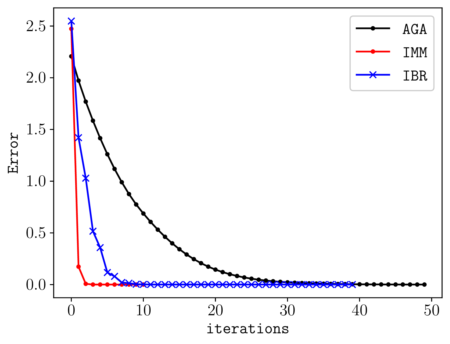
The game has a unique Nash equilibrium, which also coincides with the optimal point of the potential function. We plot the error (i.e., distance to Nash equilibrium) comparing gradient descent (AGA), iterative best response (IBR) and iterative MM (IMM) in Fig. 2, starting from the same initial point. AGA uses Nesterov’s accelerated gradient ascent scheme. From the plot it is clear that IMM converges faster than both IBR and AGA to the Nash equilibrium, and in fewer number of iterations. While IBR has lower inter-agent communication complexity that AGA, calculating the best response at each agent, may require a higher computational complexity at each agent, as opposed to gradient computation. Depending on the structure of the utility function, this may have differing complexity. In some cases it will be equivalent to solving a linear or quadratic equation. In other instances it may be that the agents have to use gradient or other learning methods locally in order to compute their best response. The minorizers for each stage of IMM were created as in definition 6, with \(\lambda=0.1\).
Application: Designing Incentives in an Energy Community↩︎
Consider an example of a collective of users buying electricity from an electricity producer. Each user buys \(x_i\) units from the producer at a price \(p_i\) per unit. Each user has a consumption threshold \(d_i\). This could, for example, represent a minimum consumption level to meet their requirements. If the purchased quantity is above this threshold, then the user benefits from the purchase; otherwise it is a loss. The individual random reward is \[\begin{align} \mathcal{R}_i(x_i,\xi)=(x_i-d_i)\xi, \end{align}\] where \(\xi\) models randomness of outcome. The collective usage benefit is \[\begin{align} \mathcal{J}(\boldsymbol{x})=-\sum_{i=1}^N(x_i-d)^2,~\mathcal{R}_i(x_i,\xi)=(x_i-d_i)\xi. \end{align}\] This represents an attempt by the collective of the users to keep the purchase vector \(\boldsymbol{x}\) close to some desired vector \((d,...,d)\). Here \(d\) represents a target energy consumption, for example, mapped from target carbon emission levels. The goal is to design incentives that drive the collective usage benefit \(\mathcal{J}(\boldsymbol{x})\) to a desired target \(\tau\). We note that it in this case, \(\mathcal{J}(\boldsymbol{x})\) is in itself strictly convex. We define the incentivized utility of the system to be \[J_i(x_i,\boldsymbol{x}_{-i})=\mathcal{J}^{\lambda_i}(\boldsymbol{x})+\mathbb{E}[V_i(\mathcal{R}_i(x_i,\xi))],\] where \(\mathcal{J}^{\lambda_i}(\boldsymbol{x})=\mathcal{J}(\boldsymbol{x})-\lambda_ix_i\), with \(\lambda_ix_i\) being a linear incentive function (since in this case there is no separate need for a regularizer, since we start with a unique equilibrium). This form of utility is a variant of 4 , and all results discussed previously will hold in this case as well. The \(\lambda_i\) are interpreted as per unit incentives/prices to users.
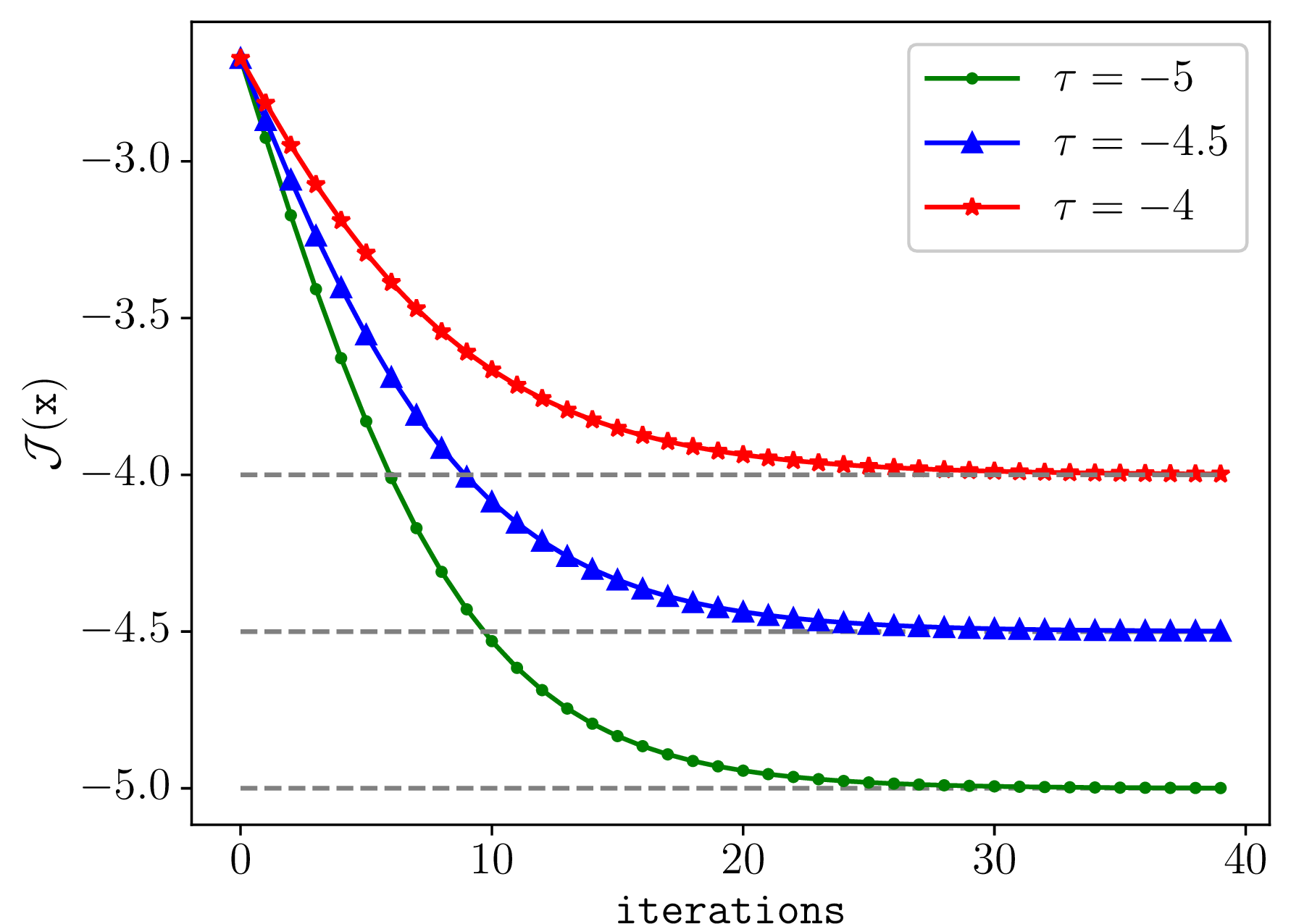
Using iterative MM, one can design a simple learning process to reach the target \(\tau\) for \(\mathcal{J}(\boldsymbol{x})\) as follows. We let the incentives evolve such that they follow a gradient of the function \((\mathcal{J}(\boldsymbol{x})-\tau)^2\), while simultaneously proceeding with MM optimization of the potential function of the game. We plot the results for a two player game, with \[V_1(x)=\log(1+x)\mathbf{1}_{(x\ge 0)}+x\mathbf{1}_{(x<0)},~V_2(x)=x,\] and parameters \(d=4\), \(d_1=1\), \(d_2=2\), and \(\xi\) supported over the set \(\{5,1\}\) with distribution \(\{0.8,0.2\}\). We plot three sample paths, all starting from the point \((x_1,x_2)=(1,1)\) with targets \(\tau=-4,-4.5\) and \(-5\).
6.2 Non Smooth Games↩︎
Convergence: Advantage of MM over Best Response↩︎
In non smooth games, MM approaches have a distinct advantage over best response based approaches. In order to demonstrate this, we consider the same non smooth game that was considered in Example 1, where we had a two agent team game with utilities \[J_1^{\lambda}(x_1,x_2)=J_1^{\lambda}(x_1,x_2)=5-|x_1+x_2|-\lambda(x_1^2+x_2^2),\] with \(\lambda=0.1\). Recall that the potential function corresponding to this game had a unique maximum at \((0,0)\), but the game had other Nash equilibria as well.
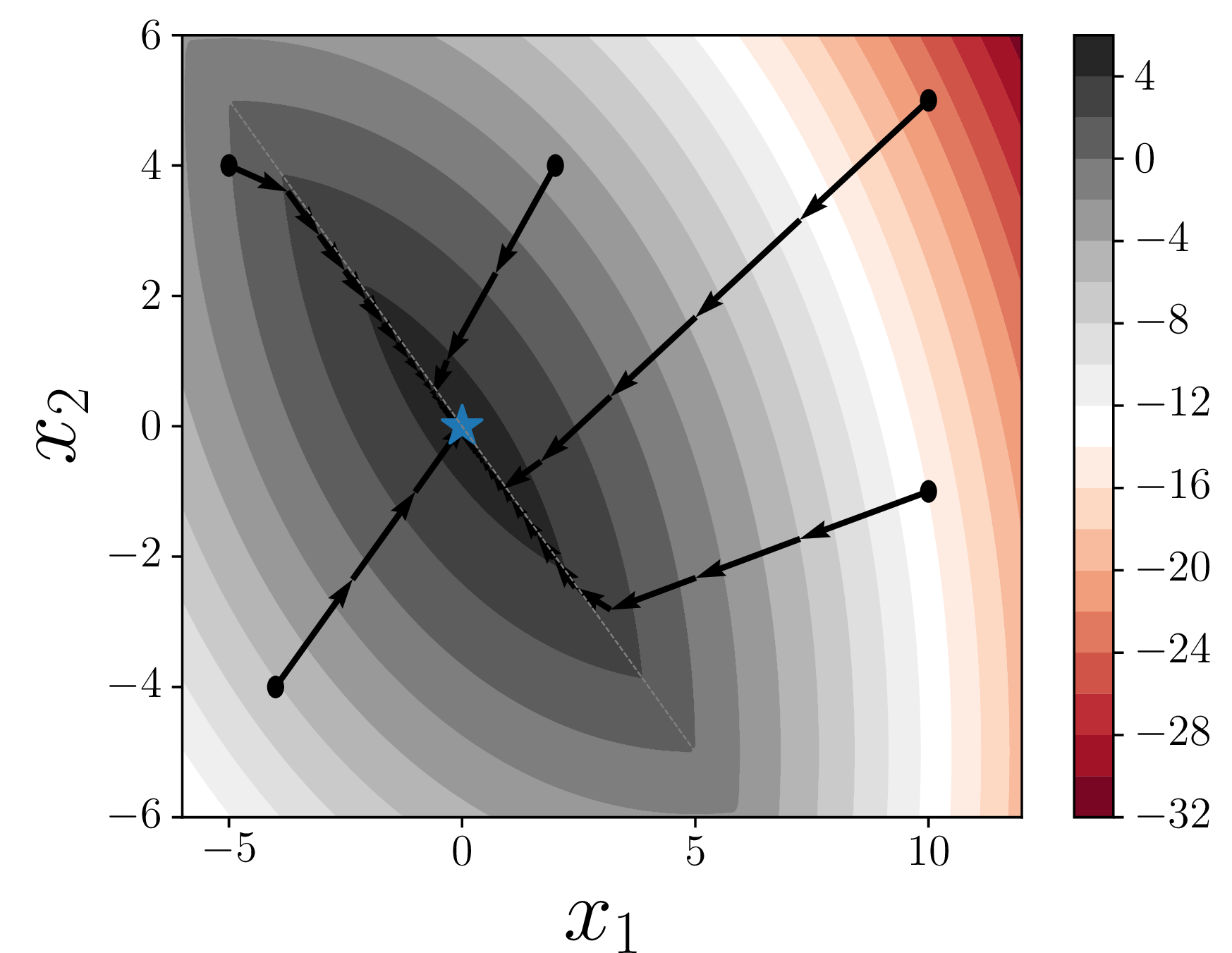
We compare the convergence behaviour of iterative MM (IMM), accelerated (sub) gradient ascent (sGA) and iterative best response (IBR) for this game. We see how the system state \(\boldsymbol{x}=(x_1,x_2)\) evolves starting from the same five initial states, \((2,4)\), \((-4,-4)\), \((-5,4)\), \((10,5)\) and \((10,-1)\). In Fig. 3, we plot the iterates of IMM, with the contours of the potential function in the background. The algorithm converges to \((0,0)\), in a rather direct matter, in a few iterations. The algorithm takes steps of large magnitude intitally, and then proceeds in smaller steps.
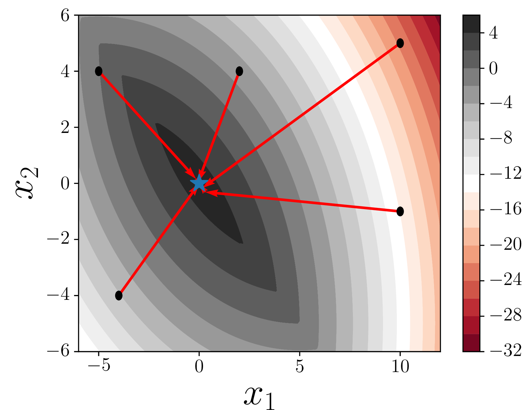
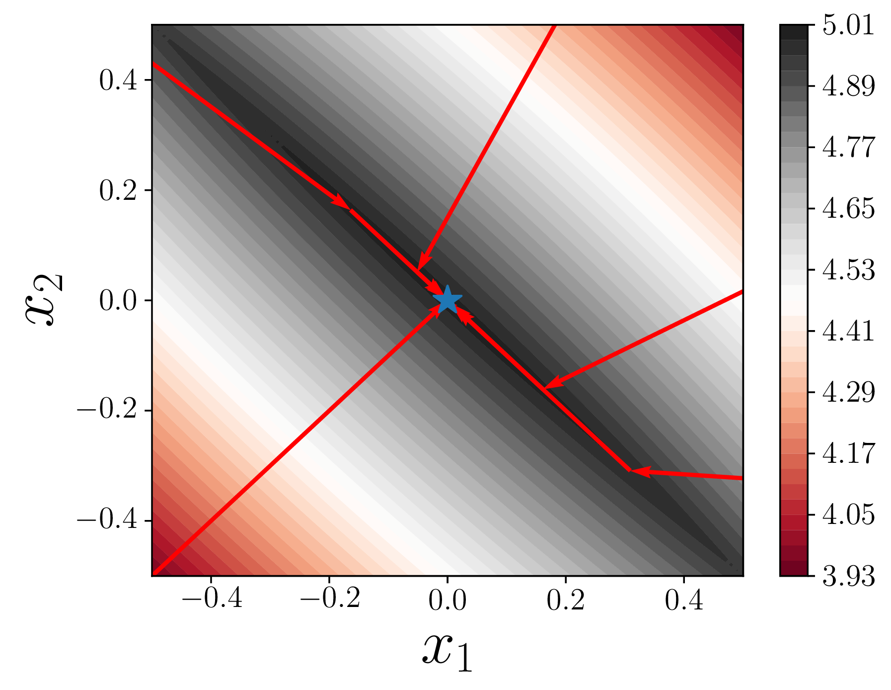
Figure 4: State evolution of iterative MM, along the contours of the potential function, starting from different initial states. On the left we have a zoomed out perspective, where we see the larger intial steps of the algorithm. On the right, we zoo in to see the finer steps of the state evolution close to the potential-optimal Nash equilibrium, represented by the blue star at \((0,0)\).. a — Zoomed out, b — Zoomed in
In the case of sGA, in Fig. 5, we see that they converge to \((0,0)\), by first reaching the line \(x_1+x_2=0\), and then ascending to \((0,0)\). Note that sGA is the same as AGA discussed previously, with the additional property that at non differentiable points, it chooses a value from the set of subdgradients as the derivative, uniformly randomly. We use a fixed small step size of 0.1 for the gradient ascent, because it allows for faster convergence than a decreasing step size. The trajectory shown is averaged over 100 sample paths.
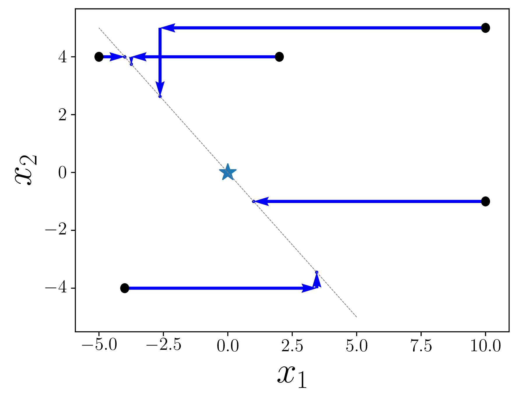
In the case of IBR in Fig. 6, we see that iterative best response leads strategies to fixed points that are Nash equilibria of the game, but not optimizers of the potential function. We see that the agents move sequentially, with agent 1 updating their startegy followed by agent 2. They cluster along the line \(x_1+x_2=0\). While IBR converges faster than sGA, it cannot move once it reaches the line \(x_1+x_2=0\).
Application: Multi Agent Distributed Learning on a Grid↩︎
We consider the problem of steering multiple agents on a grid to a common point. These could be robotic agents as in the rendezvous problem [6], [38], or vehicles coordinating their movement in a city with a Manhattan type layout [39]. We consider an example with three agents moving on the positive quadrant. Let the positions (states) of the agents be \(\boldsymbol{w}_i=(x_i,y_i)\) for \(i=1,2,3\), and the joint state be \(\boldsymbol{w}=(\boldsymbol{w}_1,\boldsymbol{w}_2,\boldsymbol{w}_3)\). We assume that agents have a cost structure of the form 4 . Let the collective benefit function be the total absolute error \[\begin{align} \mathcal{J}(\boldsymbol{w})=-\sum_{i=1}^3\sum_{j=1}^{i-1}|x_i-x_j|+|y_i-y_j|, \end{align}\] which is a measure of closeness of the agents. This benefit is maximized when all the agents coincide in their location. The \(L_1\) metric indicates that the agents are constrained to move in a grid. Each agent will also have a cost associated with its current position, which is \(C_i(x_i,y_i)\) which captures its perception of its current state. We assume that \[\begin{align} C_1(x_1,y_1) &=c_1(x_1+y_1),\\ C_2(x_2,y_2) &=c_2(2-\mathbb{E}\exp(-k_1x_2\xi)-\mathbb{E}\exp(k_2y_2\xi)),\\ C_3(x_3,y_3) &=c_3(2-\exp(-k_3x_3)-\exp(-k_4y_4)). \end{align}\] Thus agents 2 and 3 have a skewed perception of their cost. We have the utilities \[J_i(\boldsymbol{w}_i,\boldsymbol{w}_{-i})=\mathcal{J}(\boldsymbol{w})-\lambda H(\boldsymbol{w})-C_i(x_i,y_i).\] Here \(H\) is the regularizer, which we choose to be \(H(\boldsymbol{w})=\sum_{j=1}^3||\boldsymbol{w}_i||^2\). We have \(\lambda=1\),\(c_1=4\), \(c_2=0.4\), \(c_3=1\), \(k_1=0.1\), \(k_2=0.3\), \(k_3=k_4=1\), and \(\xi\) is supported over the set \(\{1,100\}\) with distribution \(\{0.9,0.1\}\). We consider two approaches to solve this, a distributed version of iterative MM (IMMd) and (sub) Gradient Ascent (SGA), with initial states \(\boldsymbol{w}_1=(10,0)\), \(\boldsymbol{w}_2=(0,10)\) amd \(\boldsymbol{w}_3=(10,10)\). We also assume that the agents are also constrained to move in the grid along one of the cardinal directions (up, down, left, right) with unit steps. In Fig. 7 (a) we show how the three robotic agents move to converge at a common point, using IMMd. In IMMd, the agents proceed in a cyclic fashion. Each one maximizes the MM surrogate locally, for a given state of the other agents. It then passes the updates state information to the next agent, which proceeds likewise. A coordinating agent is necessary to enable the intermediate communication of system states. The same process using sGA, is shown in Fig 7 (b). Using IMM, two of the agents meet much earlier on than in sGA. This suggests that IMM allows for earlier formation of clusters. We see that in sGA, at the termination, the agents do not meet at one point, but continue to move in a loop. This is a result of the synchronized and restricted grid movement with a single step at each instant, and can be remedied by de-synchronizing the agents.


Figure 7: Movement of three robotic agents starting from three different locations, for different algorithms.. a — Agents using IMMd, b — Agents using sGA
7 Conclusions and Future Work↩︎
In this paper, we studied a class of games in which agents derive utility from both a shared collective benefit and individually perceived stochastic rewards modeled via prospect theory. Such games may admit multiple equilibria, especially in the absence of regularization. To address this, we introduced a regularization framework that induces strict concavity of the potential function, ensuring the existence of a unique equilibrium. We also established a quantitative relationship between the equilibria of the regularized and unregularized games, providing insight into equilibrium selection. We then analyzed learning dynamics for computing equilibria. While gradient-based and best response methods converge in smooth settings, they may fail to reach potential-maximizing equilibria in non-smooth games. To overcome this limitation, we proposed an MM-based learning scheme, which guarantees convergence to a potential-optimal equilibrium and demonstrates improved convergence behavior. These results highlight the importance of regularization and optimization-based learning in achieving robust equilibrium selection, and suggest several directions for future work, including extensions to non-convex and more general behavioral models.
References↩︎
Inria and DI ENS, Paris, France. Email: ashok-krishnan.komalan-sindhu@inria.fr↩︎
Inria, Lille, France. Email: helene.le-cadre@inria.fr↩︎
Inria and DI ENS, Paris, France. Email: ana.busic@inria.fr↩︎
This work was supported by Défi Inria-EDF↩︎
Most of the results in this work can be extended to the case where \(\xi\) has continuous distribution, albeit with more conditions on other variables to ensure integrability. We restrict ourselves to a finite support for simplicity.↩︎
A team game is a game in which all agents have identical utility.↩︎