Ensemble Distributionally Robust Bayesian Optimisation with Continuous Context
May 08, 2026
1 Introduction↩︎
Design optimisation is fundamental to engineering and scientific discovery, aiming to identify system configurations that maximise operational efficiency or minimise costs [1]. The underlying objective function is usually unknown, expensive to evaluate, and analytically intractable. These systems are treated as black boxes - complex simulators or real-world experiments that return only point-wise values for queried inputs, offering no direct gradient information to guide the optimisation.
While black-box optimisation spans both gradient-based and gradient-free paradigms, the former is largely restricted to differentiable objectives [2], [3]. Many critical problems and applications, however, involve non-differentiable landscapes or stochastic simulators with intractable likelihoods. Examples include Monte-Carlo simulations in particle scattering [4] molecular dynamics [5] and many more. In these scenarios, Bayesian Optimisation (BO) [6] has emerged as a powerful framework for sample-efficient global optimisation.
A particularly challenging extension is contextual BO, where the objective function depends on a controllable design variable \(x \in \mathcal{X}\) and an uncontrollable environmental contextual variable \(c \in \mathcal{C}\) drawn from an unknown distribution \(P\). While the problem simplifies to standard stochastic optimisation if \(P\) is known, real problems require \(P\) to be estimated from empirical data. This estimation leads to a distributional mismatch between the true and the nominal contextual distributions, potentially resulting in sub-optimal designs.
The Distributionally Robust Optimisation paradigm safeguards against such errors [7], [8], recently finding synergy with BO [9]–[11]. DRO utilises statistical divergences or distance metrics to construct an ambiguity set - a family of candidate distributions centred around the nominal one. By optimising for the worst-case scenario within this set, DRO provides a robust lower bound on performance, ensuring reliability even under distributional shifts.
Contributions. Our primary contributions are as follows:
We propose Ensemble Distributionally Robust Bayesian Optimisation (EDRBO), a novel framework that integrates ensemble learning with DRO to model both the black-box function and the associated distributional uncertainty without requiring restrictive assumptions on the ambiguity set or the context space. Our approach leverages the properties of Wasserstein DRO to derive a computationally tractable acquisition function, effectively resolving the maximin challenge inherent in DRO while preserving efficiency required for practical application.
We provide a rigorous theoretical analysis, deriving a desired sublinear cumulative regret order of \(\mathcal{O}(\gamma_T \sqrt{T})\), where \(T\) represents the time horizon and \(\gamma_T\) denotes the maximum information gain within the ensemble.
We demonstrate the efficacy of EDRBO through extensive experiments, showing that it consistently matches or outperforms state-of-the-art methods while maintaining computational tractability.
The main text of this paper is organised as follows. Section 2 establishes the necessary preliminaries. In Section 3, we detail the EDRBO framework and present our theoretical results. Finally, Section 4 provides an empirical evaluation and discussion of our findings.
Notation. We denote the search space by \(\mathcal{X} \subseteq \mathbb{R}^{d_x}\) and the context space by \(\mathcal{C} \subseteq \mathbb{R}^{d_c}\). We make a common and mild assumption that \(\mathcal{X}\) is compact. Let \(\Xi = \mathcal{X} \times \mathcal{C}\) and \(\xi = [x^T, c^T]^T\). The black-box function \(f: \Xi \rightarrow \mathbb{R}\) is assumed to be bounded from above. The ensemble surrogate model \(\hat{f}\) is comprised of \(M\) distinct constituent surrogates \(\hat{f}_m\). Each is defined by a positive semi-definite kernel \(k_m: \Xi \times \Xi \rightarrow \mathbb{R}\) with \(\mathcal{H}_m\) being the unique RKHS associated with the kernel, equipped with norm \(\|\cdot\|_{\mathcal{H}_m}\); \(k_m\) is \(L_m(x)\)-Lipschitz with respect to \(c\) and \(L_m(x) > 0\) \(\forall x \in \mathcal{X}\). We assume that \(\|f\|_{\mathcal{H}_m} \leq B_m, B_m > 0\) and that \(\forall \xi, \xi' \in \Xi \;\;k_{m}(\xi, \xi')\leq 1\). We use \(\mathbb{P}(\mathbb{R}^{d_c})\) to denote the set of all Borel probability measures on \(\mathbb{R}^{d_c}\), and \(\mathbb{P}_2(\mathbb{R}^{d_c}) \subset \mathbb{P}(\mathbb{R}^{d_c})\) the subset of measures with finite second moment. We use \(f(x, \cdot) \# Q\) to denote the push-forward of the context distribution \(Q\) through \(f\). We denote the iteration budget by \(T\). At iteration \(t\) we use \(\mathbb{D}_{t} = \{(x_{\tau}, c_{\tau}, y_{\tau})\}_{\tau=1}^t\) for the set of ground truth values and \(\epsilon_t\) to denote the zero-mean \(R\)-sub-Gaussian output noise. We denote expected regret at iteration \(t\) by \(r_t\) and the cumulative expected regret is defined as \(R_T = \sum_{t=1}^T r_t\). To describe asymptotic behaviour regret bounds we use the big O notation: \(\mathcal{O}(\cdot)\).
2 Preliminaries↩︎
2.1 Bayesian Optimisation↩︎
Consider a black-box function \(f\) to be optimised with respect to the design variable \(x\). \(f\) is point-wise observable and there is no direct access to neither \(f\) nor its gradients. At each iteration, \(t\), the learner selects a design \(x_t \in \mathcal{X}\), observes context \(c_t \in \mathcal{C}\) and a noisy observation of \(f: y_t = f(x_t, c_t) + \epsilon_t\). The context variable \(c \sim P \in \mathbb{P}_2(\mathbb{R}^{d_c})\), \(P\) is chosen by the environment and is unknown to the learner. The goal is to find the global maximiser of \(f\):
\[x^* = \mathop{\mathrm{arg\,max}}_{x \in \mathcal{X}} \mathbb{E}_{c \sim P} [f(x, c)] .\]
The \((x_t, c_t, y_t)\) triplets comprise the set of all ground truth values obtained up to iteration \(t\), \(\mathbb{D}_t\). At iteration \(t\), \(f\) is modelled by a surrogate model \(\hat{f}\) fit on \(\mathbb{D}_t\). Using the surrogate’s approximation, BO builds an acquisition function to guide the optimisation. By optimising the acquisition function, one identifies promising regions of the search space, while accounting all that is known and unknown regarding the objective function at current iteration.
2.2 Surrogate model↩︎
Consider an ensemble of \(M\) Gaussian processes. Following [9], [11], each base expert solves a regularised least-squares problem in its RKHS. For regularisation parameter \(\lambda > 0\), at iteration \(t\), given \(\mathbb{D}_t\), the posterior mean is given by
\[\label{eq:mean} \mu_{m,t}(\xi) = \boldsymbol{k}_{m,t}(\xi)^T \left( \boldsymbol{K}_{m,t} + \lambda \boldsymbol{I}\right)^{-1} \boldsymbol{y}_t\tag{1}\] and covariance \[\label{eq:cov} k_{m,t}(\xi, \xi') = \frac{1}{\lambda} \left( k_m(\xi, \xi') - \boldsymbol{k}_{m,t}(\xi)^T \left( \boldsymbol{K}_{m,t} + \lambda \boldsymbol{I}\right)^{-1} \boldsymbol{k}_{m,t}(\xi') \right),\tag{2}\] where \(\boldsymbol{k}_{m,t}(\xi) = [k_m(\xi, \xi_1), \ldots, k_m(\xi, \xi_t)], \boldsymbol{K}_{m, t}\) is the kernel Gram matrix, and \(\boldsymbol{y}_t = [y_1, \ldots, y_t]\). To approximate the black-box function we average the expert mean: \[\label{eq:bbf95mean95approx} \hat{f}(\xi) = \mu_t(\xi) = \frac{1}{M} \sum_{m=1}^M \mu_{m, t}(\xi),\tag{3}\] for which we provide the following finite-sample confidence guarantees.
Lemma 1. Let \(\Xi \in \mathbb{R}^d\) and \(f: \Xi \rightarrow \mathbb{R}\). Each expert assumes that \(f \in \mathcal{H}_m\), with \(\|f\|_{\mathcal{H}_m} \leq B_m\) and let \(\epsilon_t\) be \(R\)-sub-Gaussian. Let \(\delta \in (0, 1)\). With probability at least \(1-\delta\), \(\forall \xi \in \Xi\) and \(\forall t\geq 1\): \[|\mu_t(\xi) - f(\xi)| \leq \beta_t \sigma_t(\xi),\] with \[\label{eq:std95approx} \sigma_t(\xi) = \frac{1}{M} \sum_{m=1}^M \sigma_{m, t} (\xi)\qquad{(1)}\] and \[\label{eq:beta95max} \beta_t = \max_m B_m + R \sqrt{2\left(\gamma_{m,t} + 1 + \log \frac{M}{\delta}\right)},\qquad{(2)}\] where \(\gamma_{m,t}\) is maximum information gain. A full proof is provided in Appendix 6.1.
For ensemble methods to be effective, the orthogonality, or distinctness, of its base experts is vital. Gaussian processes are fundamentally either equivalent or orthogonal, end even under equivalence, they yield varying predictions for finite data [12]. By the Feldman-Hájek theorem [13], [14], distinct base experts, residing in distinct RKHSs, are orthogonal. We employ the following kernels: Square Exponential, Rational Quadratic, and Matérn kernels with \(\nu=\frac{3}{2}\) and \(\nu=\frac{5}{2}\). While they cover the standard suite of Lipschitz kernels, the future scalability of such ensembles pose an interesting challenge for both the theoretical and empirical aspects of the model.
2.3 Maximum information gain↩︎
Design points are chosen to obtain the best possible estimates of the black-box function, while attempting to learn \(f\) in as few iterations as possible. The reduction in uncertainty about \(f\) from observing \(\boldsymbol{y}_t\) is called information gain and is the mutual information between \(f\) and observed outputs \(\boldsymbol{y}_t\), i.e., \(\mathcal{I}(\boldsymbol{y}_t; f)\). In general, finding its maximiser is NP-hard [15]. For a Gaussian predictive posterior the problem \[\label{eq:mig} \gamma_t \stackrel{\mathclap{\scriptsizedef}}{=}\max_{\mathbb{D}_t} \; \mathcal{I}(\boldsymbol{y}_t; f)\tag{4}\] is equivalent to choosing the variance-maximising design [16]. Thus, maximum information gain takes the following form: \[\label{eq:gauss95mig} \gamma_t = \max_{\mathbb{D}_t} \log \det (\boldsymbol{I} + \lambda^{-1} \boldsymbol{K}_{m,t}),\tag{5}\] where \(\boldsymbol{K}_{m,t}\) is the posterior covariance of a Gaussian process surrogate over \(\mathbb{D}_t\).
2.4 Distributionally Robust Optimisation↩︎
The true context distribution \(P\) is fundamentally unknown. The learner only observes finite samples of context and estimates a nominal distribution \(Q_t\). But with finite data this estimate is subject to statistical error, which is impossible to overcome due to the optimiser’s curse [8].
The DRO paradigm completely mitigates this by employing a set of plausible context distributions. We focus on a common choice of such ambiguity sets - Wasserstein balls. Specifically, we consider the \(2\)-Wasserstein distance as the DRO metric, which results in the following ambiguity set centred at \(Q_t\) and radius \(\varepsilon_t \geq 0\):
\[\label{eq:ball} \mathbb{B}_{\varepsilon_t}(Q_t) \stackrel{\mathclap{\scriptsizedef}}{=}\{ Q \in \mathbb{P}_2 : W_2(Q, Q_t) \leq \varepsilon_t \}.\tag{6}\]
The radius \(\varepsilon_t\) acts as a tolerance on the distributional deviation. Now, the learner has to find the best design against the worst-case distribution within the ambiguity set, which yields the following maximin problem:
\[\label{eq:dro95obj} \max_{x \in \mathcal{X}} \;\inf_{Q \in \mathbb{B}_{\varepsilon_t}(Q_t)} \;\mathbb{E}_{c \sim Q}[f(x, c)].\tag{7}\]
3 Method↩︎
The key component of BO is the acquisition function. There are several established technique, most notably the Confidence Bound approach, which leverages the trade off between exploitation, \(\mu_t\), and exploration, \(\sigma_t\). Directly optimising \(\mu_t\) is a good worst-case bound for \(f\) [17], which may be too greedy, has no mechanism to escape suboptimal solutions, and does not incorporate uncertainty in any form [16]. Motivated by Lemma 1, consider the following learner problem: \[\label{eq:inital95acqf} x_t = \mathop{\mathrm{arg\,max}}_{x \in \mathcal{X}} \inf_{Q \in \mathcal{B}_{\varepsilon_t}(Q_t)} \mathbb{E}_{c \sim Q} [\mu_t(x, c) + \beta_t \sigma_t(x, c)].\tag{8}\] As the entirety of contextual information is encapsulated in the limited observed context samples, we take advantage of the chosen surrogate model. First, consider a meaningful consensus of base experts with respect to the Wasserstein geometry - the Wasserstein Barycentre, which is the solution to the problem: \[\bar{f}_t(\xi) = \mathop{\mathrm{arg\,min}}_{\bar{f}} \frac{1}{M} \sum_{m=1}^M W_2(\hat{f}_{m,t}(\xi), \bar{f}(\xi)).\] In general, finding \(\bar{f}(\xi)\) is NP-hard [18]. However, since the posterior of base experts is \(1\)D Gaussian, the ensemble barycentre is analytically tractable. It remains Gaussian, \(\bar{f}_t(\xi) \sim \mathcal{N}(\bar{\mu}_t(\xi), \bar{\sigma}_t^2(\xi))\), with \(\bar{\mu}_t(\xi) = M^{-1} \sum_{m=1}^M \mu_{m, t}(\xi)\) and \(\bar{\sigma}_t(\xi) = M^{-1} \sum_{m=1}^M \sigma_{m, t}(\xi)\). The barycentre effectively averages base experts instead of linearly mixing their densities.
The closed form of the barycentre comes in hand to define an exploration budget based on context gap. Consider the posterior radius as the largest \(2\)-Wasserstein distance between a single base expert and the ensemble barycentre. Leveraging the closed-form Bures-Wasserstein distance for Gaussians, the radius also breaks down intro epistemic and aleatoric uncertainty of the ensemble: \[\begin{align} \label{eq:radius} \hat{\varepsilon}_t(\xi) &\stackrel{\mathclap{\scriptsizedef}}{=}\max_{m} W_2(\hat{f}_{m,t}(\xi), \bar{f}_t(\xi))=\\ &=\max_{m} \sqrt{ \underbrace{(\mu_{m,t}(\xi) - \bar{\mu}_t(\xi))^2}_{\text{Structural Disagreement}} + \underbrace{(\sigma_{m,t}(\xi) - \bar{\sigma}_t(\xi))^2}_{\text{Confidence Dispersion}}}. \end{align}\tag{9}\] To simplify the DRO problem, first consider the following Wasserstein robust regulariser:
Lemma 2 (Lemma 2 by [19]). For an \(L(x)\)-Lipschitz function \(g\), \(\forall x \in \mathcal{X}\), \(\forall Q \in \mathbb{B}_{\varepsilon_t}(Q_t)\) and \(\forall t \geq 1\): \[|\mathbb{E}_{c \sim Q}[g(x, c)] - \mathbb{E}_{c \sim Q_t}[g(x, c)]| \leq \varepsilon_t L(x).\]
For all \(x \in \mathcal{X}\) and \(\forall t \geq 1\), since \(k_m\) is \(L_m(x)\)-Lipschitz, by Lemma 3 of [11], \(\mu_{m,t}\) and \(\beta_{m,t}\sigma_{m, t}\) are \(\lambda^{-\frac{1}{2}}\beta_{m, t}L_m(x)\) - Lipschitz. Then \(\mu_t\) and \(\beta_t \sigma_t\) are \(\lambda^{-\frac{1}{2}}\beta_{t} \max_m L_m(x)\)-Lipschitz, and hence \(\mu_{t} + \beta_t \sigma_t\) is \(L(x)\) - Lipschitz with \(L(x) = 2 \lambda^{-\frac{1}{2}}\beta_{t} \max_m L_m(x)\). Since \(\beta_t \geq 1\), \(\hat{\varepsilon}_t\) is \(L(x)/\sqrt{2}\)-Lipschitz. For the posterior radius to be fit to serve the learner, we show the following result.
Theorem 1. Let \(\mu_t +\beta_t \sigma_t\) be \(L(x)\)-Lipschitz. Then \(\forall x \in \mathcal{X}\) and \(\forall t \geq 1\) the ensemble posterior radius \(\hat{\varepsilon}_t\), Eq. 9 , is bounded as: \[\frac{1}{\sqrt{2}} \varepsilon_t L(x) \leq \mathbb{E}_{c \sim Q_t} [\hat{\varepsilon}_t(x, c)] \leq \frac{3}{2\sqrt{2}} \varepsilon_t L(x).\] A full proof is provided in Appendix 6.2.
By applying Lemma 2 in combination with Theorem 1 to the non-robust acquisition function, Eq. 8 , we may discard the inherit maximin DRO problem, and get the following computationally tractable acquisition function for the learner: \[\label{eq:actual95acqf} x_t = \mathop{\mathrm{arg\,max}}_{x \in \mathcal{X}} \mathbb{E}_{c \sim Q_t}\left[\mu_t(x, c) +\beta_t \sigma_t(x, c) - \hat{\varepsilon}_t(x, c) \sqrt{2} \right].\tag{10}\] This distributionally robust acquisition function offers a fundamental improvement over existing approaches, such as [11], [20]. \(W_2(P, Q_t)\) is governed only by observed context samples. Instead of assuming and setting some rate of decay of \(\varepsilon_t\), without any guarantees, the ensemble posterior radius, \(\hat{\varepsilon}_t\), naturally decays from one iteration to another as \(W_2(P, Q_t) \rightarrow 0\). Moreover, in contrast with the standard single GP paradigm, the proposed acquisition function also captures model-based epistemic uncertainty, and thus naturally protects from exploring in search space regions where base experts conflict. Based on the proposed acquisition function we define the EDRBO algorithm in Algorithm 1.
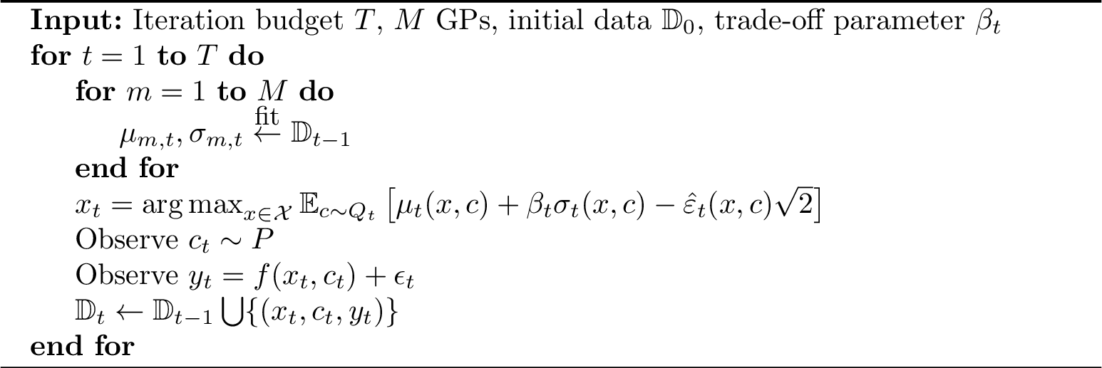
We use regret, i.e., the difference between a prediction and the oracle, to measure the performance of the algorithm. The choice of oracle and the definition of regret is not unique. To obtain a consistent comparison with existing approaches, following [20] and [11], we take the definition of instantaneous expected regret. It captures the sub-optimality gap between an algorithm and the solution of the true stochastic optimisation problem with full knowledge of the black-box function \(f\) and the true contextual distribution \(P\): \[\begin{align} \label{eq:regret} r_t &= \mathbb{E}_{c \sim P}[f(x^*, c)] - \mathbb{E}_{c \sim P}[f(x_t, c)], \\ x^* &= \mathop{\mathrm{arg\,max}}_{x \in \mathcal{X}} \mathbb{E}_{c \sim P} [f(x, c)]. \end{align}\tag{11}\]
For the proposed acquisition function, Eq. 10 , we achieve the following sublinear cumulative regret bounds, that improve on state-of-the-art results.
Theorem 2. Let \(\delta \in (0, 1)\) be a probability of failure, \(\mu_t +\beta_t \sigma_t\) be \(L(x)\)-Lipschitz, and \(\ell = \max_{x \in \mathcal{X}} L(x) / \min_{x \in \mathcal{X}} L(x)\). Then with probability at least \(1 - \delta\), \(\forall t \geq 1\) the cumulative expected regret of Algorithm 1 with \(M\) surrogates after \(T\) steps is bounded by:
\[R_T \leq 22 \ell \beta_T \sqrt{T\left(M \gamma_T + 2\log \frac{6}{\delta}\right)},\]
which results in the \(\mathcal{O}(\gamma_T \sqrt{T})\) general order of cumulative regret, where \(\gamma_T\) is the worst-case maximum information gain. A full proof is provided in Appendix 6.3.
4 Experiments↩︎
Our algorithm, EDRBO, follows the steps outlined in Section 3 and Algorithm 1. To see how it stacks up, we compare it against a variety of benchmarks that incorporate context and robustness in different ways, ranging from simple empirical models to more rigorous distributionally robust frameworks.
The UCB algorithm [16] serves as our most straightforward baseline since it skips the context variable entirely. Instead, it uses a Gaussian process to model rewards and optimizes the resulting upper confidence bound. This makes it a useful check to see if modelling context actually adds value to a specific problem or if a simpler approach suffices.
The rest of baselines include most commonly used DRBO methods. The integration of DRO into the BO framework was pioneered by [9]. DRBO-MMD works by discretizing the context space and finding a solution that holds up against the worst-case distribution within a set MMD budget. While they show that the problem could be formulated for any divergence \(\Delta\), their reliance on Maximum Mean Discrepancy creates significant scaling issues; the resulting minimax problem becomes computationally prohibitive unless the context space is kept discrete and low-dimensional.
Since DRBO-MMD can be computationally heavy, DRBO-MMD Minmax [21] offers a faster alternative. They employ Taylor expansions to conduct minmax sensitivity analysis across various ambiguity sets to achieve finer discretization without the same heavy computational overhead. Both DRBO-MMD and DRBO-MMD Minmax methods have linear regret bounds with respect to the iteration budget, limiting their long-term performance guarantees.
On the other hand, [10] focus on tractability. They extend the DRBO framework to \(\varphi\)-divergences such as Kullback-Leibler divergence and Total Variation distance. They prove that the minimax problem can be reduced to a simpler single-stage optimisation problem, thus making the algorithm much more practical. Nevertheless, their approach introduces implicit constraints regarding the support of the distributions within the ambiguity set. To handle the challenges of continuous context without relying on discretisation, SBO-KDE [20] estimates the context distribution using kernel density estimation and then maximizes the expected UCB through sampling from this estimate within a \(\varphi\)-divergence DRBO setup. Since these density estimates can sometimes be unreliable, DRBO-KDE [20] adds a layer of protection by placing a total variation ambiguity set around the estimated distribution. This hedging makes the method more resilient to potential model misspecification.
StableOpt [22] takes a different view by looking at robustness through the lens of stability. It identifies the best design by looking for the one that performs best even under the worst plausible context in a set \(C_t\). As suggested by [20], we define this set using intervals based on the empirical mean and variance of the context dimensions. This gives us a minimax perspective that explicitly guards against statistically likely but unfavorable context shifts.
Most recently [11] applied Wasserstein DRO to robustify the BO confidence bound acquisition function. Much like [10], they bypass the maximin bottleneck by utilising the Lipschitz properties of the objective function over Wasserstein balls, i.e., the Wasserstein DRO ambiguity set. Their work effectively fills a gap in the literature concerning continuous context distributions. WDRBO [11], which creates a Wasserstein ambiguity set around the observed contexts. The radius of this set, \(\varepsilon_t = O(1/\sqrt{t})\), naturally tightens as more data arrives, making the model less conservative over time. As a point of comparison, we also include ERBO [11], which is essentially a non-robust version of WDRBO that sets the radius to zero. By simply maximizing the average performance across observed contexts, ERBO serves as a context-aware but non-robust baseline.
| Method | Three-Hump Camel | Six-Hump Camel | Ackley | Hartmann | Complicated Hartmann |
|---|---|---|---|---|---|
| EDRBO (Ours) | 2.9 \(\pm\) 0.5 | 96.34 \(\pm\) 85.47 | 195.02 \(\pm\) 67.8 | 62.73 \(\pm\) 30.08 | 70.93 \(\pm\) 36.8 |
| SBO-KDE | 3.13 \(\pm\) 1.09 | 105.08 \(\pm\) 81.19 | 332.33 \(\pm\) 160.31 | 79.05 \(\pm\) 53.63 | 93.89 \(\pm\) 62.65 |
| UCB | 5.44 \(\pm\) 2.03 | 81.23 \(\pm\) 56.36 | 318.12 \(\pm\) 151.63 | 112.51 \(\pm\) 65.41 | 125.46 \(\pm\) 69.64 |
| WDRBO | 3.39 \(\pm\) 1.11 | 145.8 \(\pm\) 65.43 | 409.87 \(\pm\) 175.31 | 72.6 \(\pm\) 36.98 | 88.49 \(\pm\) 44.9 |
| ERBO | 3.15 \(\pm\) 1.06 | 107.7 \(\pm\) 83.5 | 269.17 \(\pm\) 127.19 | 66.9 \(\pm\) 35.55 | 75.35 \(\pm\) 43.37 |
| DRBO-KDE | 3.44 \(\pm\) 1.31 | 106.68 \(\pm\) 82.88 | 377.28 \(\pm\) 171.38 | 94.97 \(\pm\) 58.46 | 106.97 \(\pm\) 58.22 |
| StableOpt | 30.81 \(\pm\) 18.31 | 178.98 \(\pm\) 65.19 | 734.37 \(\pm\) 388.01 | 185.61 \(\pm\) 99.74 | 173.42 \(\pm\) 92.84 |
| DRBO-MMD | 5.38 \(\pm\) 1.96 | 129.74 \(\pm\) 36.26 | 510.58 \(\pm\) 217.32 | 153.08 \(\pm\) 70.14 | 159.04 \(\pm\) 76.65 |
| DRBO-MMD Minmax | 7.08 \(\pm\) 2.99 | 248.36 \(\pm\) 103.97 | 599.73 \(\pm\) 303.7 | 161.13 \(\pm\) 78.21 | 159.01 \(\pm\) 76.64 |
| Method | Modified Branin | Newsvendor | Portfolio (Uniform) | Portfolio (Normal) | Average rank |
|---|---|---|---|---|---|
| EDRBO (Ours) | 726.01 \(\pm\) 257.04 | 6.89 \(\pm\) 1.61 | 299.11 \(\pm\) 120.27 | 420.49 \(\pm\) 171.92 | 1.22 \(\pm\) 0.44 |
| SBO-KDE | 754.6 \(\pm\) 309.47 | 9.6 \(\pm\) 2.63 | 325.17 \(\pm\) 105.61 | 447.37 \(\pm\) 160.39 | 2.89 \(\pm\) 0.93 |
| UCB | 908.2 \(\pm\) 460.49 | 12.07 \(\pm\) 5.5 | 358.22 \(\pm\) 134.73 | 574.02 \(\pm\) 293.95 | 5.00 \(\pm\) 1.94 |
| WDRBO | 807.67 \(\pm\) 233.47 | 10.71 \(\pm\) 3.43 | 373.11 \(\pm\) 138.79 | 505.98 \(\pm\) 202.28 | 4.44 \(\pm\) 1.33 |
| ERBO | 685.02 \(\pm\) 266.35 | 10.44 \(\pm\) 3.45 | 347.44 \(\pm\) 105.25 | 448.87 \(\pm\) 169.05 | 2.67 \(\pm\) 1.12 |
| DRBO-KDE | 883.97 \(\pm\) 313.51 | 11.63 \(\pm\) 4.05 | 437.22 \(\pm\) 179.21 | 533.35 \(\pm\) 224.77 | 5.00 \(\pm\) 0.5 |
| StableOpt | 2301.76 \(\pm\) 1461.35 | 45.27 \(\pm\) 24.17 | 734.99 \(\pm\) 366.79 | 807.47 \(\pm\) 354.31 | 8.78 \(\pm\) 0.44 |
| DRBO-MMD | 987.42 \(\pm\) 371.17 | 36.18 \(\pm\) 15.76 | 597.6 \(\pm\) 247.67 | 644.69 \(\pm\) 255.29 | 6.89 \(\pm\) 0.6 |
| DRBO-MMD Minmax | 1241.81 \(\pm\) 588.03 | 47.0 \(\pm\) 24.36 | 644.61 \(\pm\) 254.66 | 691.56 \(\pm\) 296.39 | 8.11 \(\pm\) 0.6 |
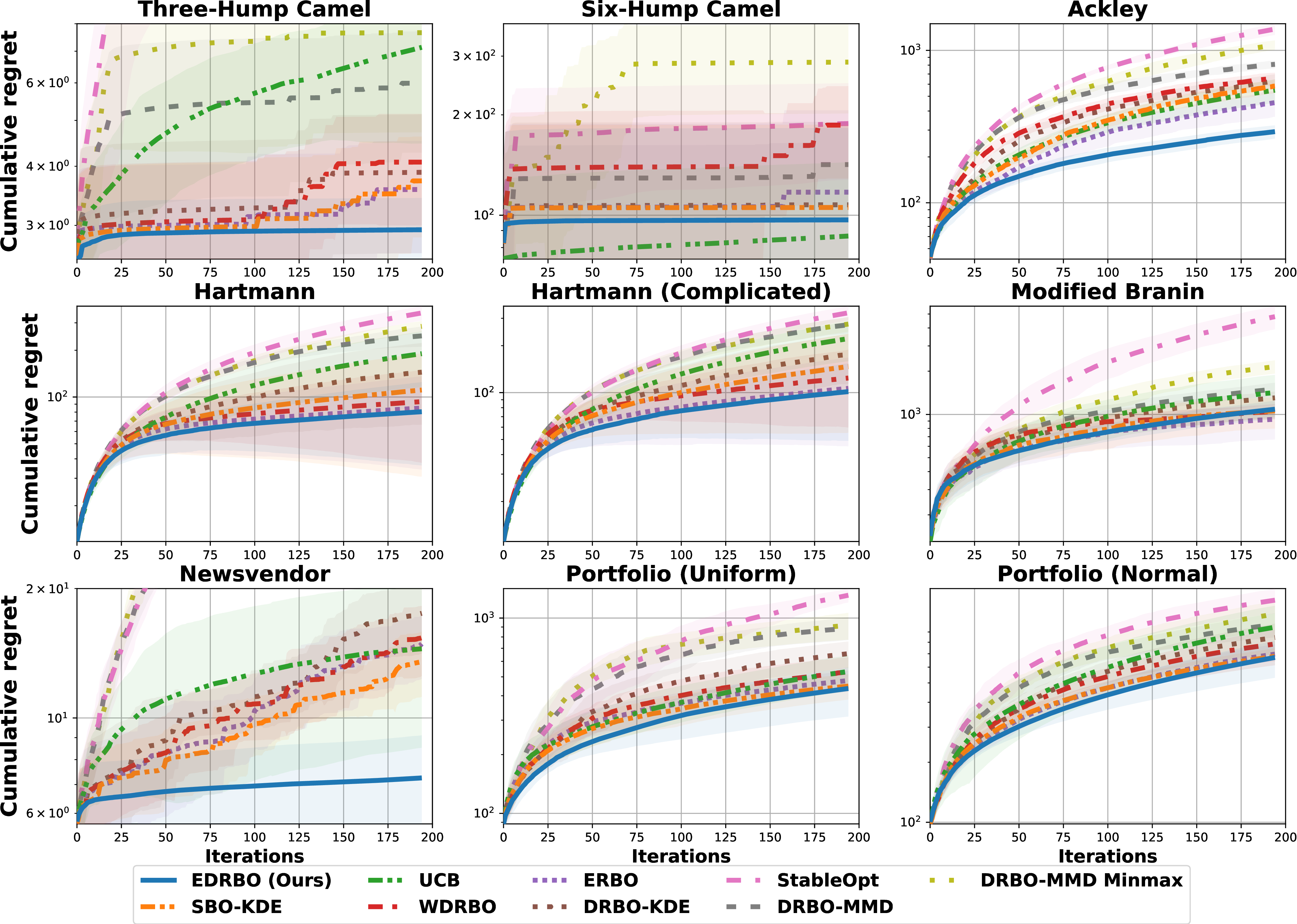
We test the algorithms on a range of synthetic and real-world problems with various context distributions. Each algorithm runs for \(200\) iterations, including \(5\) starting points, at \(10\) different random seeds. Fig. 2 presents the mean and standard deviation of cumulative regret over these runs. The final values of cumulative regret are presented in Table ¿tbl:tab:results?. We adapt existing experimental setups [11], [20]. A detailed description of all experiments can be found in Appendix 7.
Empirical results provide significant insight into how EDRBO compares with existing approaches. The method achieves the best average ranking of \(1.22\) across all experiments. Specifically, EDRBO produces the best result in all experiments but Six-Hump Camel and Modified Branin, where it is second only to UCB and ERBO, respectively. Simultaneously, these methods together with WDRBO have the largest rank standard deviations, which make them most inconsistent. While EDRBO notably prevails over baseline methods on Three-Hump Camel, Ackley, and Newsvendor functions, it improves marginally on the rest, which leads to the following insights.
The main advantage of EDRBO is its handling of highly non-convex landscapes with multiple local extrema. In this case, optimisation typically takes place near vanishing gradients regions. Lipschitz-based regularised methods, such as WDRBO, rely on a linear growth assumption, which makes them less stable in these areas. In more severe scenarios, where the cost landscape exhibits localised, sharply varying structures, e.g., Ackley function, the expected cost (\(\mu\)) and the predictive uncertainty (\(\sigma\)) become strongly intertwined. In contrast to standard DRBO baselines that mostly regularise only first-order deviations, EDRBO’s use of the Bures–Wasserstein distance yields a joint second-order stability guarantee.
One may observe this behaviour in the cumulative regret plots. Most noticeably for SBO-KDE and WDRBO baselines on both Camel and Newsvendor functions. While the proposed method produces a stable and smooth curve, existing DRBO methods tend to produce a jagged, staircase-like result.
We also note experiments where the interaction between decision variables and context is strongly nonlinear and non-separable. A key example is the modified Branin function. Similarly, in the Portfolio optimization problems, the objective is not given analytically but instead arises as the posterior mean of a Gaussian process fitted to sampled data. This leads to nonstationary smoothness, local irregularities, and artifacts from finite data.
In conclusion, the proposed method is optimally suited for iterative decision-making under contextual uncertainty in environments where the objective function is: (i) highly non-convex, leading to frequent occurrences of stationary points, and (ii) sensitive to joint first- and second-order moment variations.
5 Conclusions↩︎
In this work, we present Ensemble Distributionally Robust Bayesian Optimisation, a new model-driven algorithm for sequential decision making under context distributional uncertainty with no restrictive assumptions on context. The method relies on robustifying the acquisition function using Lipschitz regularisation within the Wasserstein ambiguity set and subsequent estimation that exploits the choice of surrogate - an ensemble model. In contrast with many existing distributionally robust approaches, ours yields a tractable optimisation problem in practice, while being capable of handling continuous context and having cumulative expected regret guarantees that improve on state-of-the-art methods. On a wide range of problems EDRBO attains superior to existing approaches performance, thus attesting to the theoretical results.
6 Missing Proofs↩︎
6.1 Regression confidence guarantees↩︎
To prove Lemma 1 we require the following lemma:
Lemma 3 (Theorem 2 of [23]). Let \(k: \Xi \times \Xi \rightarrow \mathbb{R}\) be the positive semidefinite kernel defining the GP surrogate, with RKHS \(\mathcal{H}_k\) and norm \(\|\cdot\|_{\mathcal{H}_k}\). Let \(f: \Xi \rightarrow \mathbb{R}\), \(f \in \mathcal{H}_k\), \(\|f\|_{\mathcal{H}_k} \leq B_m\), and let \(\epsilon_t\) be \(R\)-sub-Gaussian. Let \(\delta \in (0, 1)\) be a probability of failure. Then with probability at least \(1 - \delta\), \(\forall \xi \in \Xi\) and \(\forall t\geq 1\)
\[|\mu_{m,t}(\xi) - f(\xi)| \leq \beta_{m,t} \sigma_{m,t}(\xi),\]
with
\[\label{eq:beta95single} \beta_{m,t} = B_m + R \sqrt{2\left(\gamma_{m,t} + 1 + \log \frac{1}{\delta}\right)}\qquad{(3)}\]
Lemma 4 (Lemma 1 in the main text). Let \(\Xi \in \mathbb{R}^d\) and \(f: \Xi \rightarrow \mathbb{R}\). Each expert assumes that \(f \in \mathcal{H}_m\), with \(\|f\|_{\mathcal{H}_m} \leq B_m\) and let \(\epsilon_t\) be \(R\)-sub-Gaussian. Let \(\delta \in (0, 1)\) be a probability of failure. With probability at least \(1-\delta\), \(\forall \xi \in \Xi\) and \(\forall t\geq 1\): \[|\mu_t(\xi) - f(\xi)| \leq \beta_t \sigma_t(\xi),\] with \[\sigma_t(\xi) = \frac{1}{M} \sum_{m=1}^M \sigma_{m, t} (\xi)\] and \[\beta_t = \max_m B_m + R \sqrt{2\left(\gamma_{m,t} + 1 + \log \frac{M}{\delta}\right)}.\]
Proof. \[\begin{align} \lvert \mu_t(\xi) - f(\xi) \rvert &= \left\lvert \frac{1}{M} \sum_{m=1}^M \mu_{m,t}(\xi) - \frac{1}{M} \sum_{m=1}^M f(\xi) \right\rvert = \\ &= \left\lvert \frac{1}{M} \sum_{m=1}^M \left( \mu_{m,t}(\xi) - f(\xi) \right) \right\rvert \leq \\ & \overset{ \mathrm{\makebox[0pt]{(i)}} \def\@currentlabel{(i)} \ltx@label{l3_1_1} }{ \leq } \frac{1}{M} \sum_{m=1}^M \left\lvert \mu_{m,t}(\xi) - f(\xi) \right\rvert \leq \\ & \overset{ \mathrm{\makebox[0pt]{(ii)}} \def\@currentlabel{(ii)} \ltx@label{l3_1_2} }{ \leq } \frac{1}{M} \sum_{m=1}^M \beta_{m,t} \sigma_{m,t}(\xi) \leq \\ & \overset{ \mathrm{\makebox[0pt]{(iii)}} \def\@currentlabel{(iii)} \ltx@label{l3_1_3} }{ \leq } \beta_t \sigma_t(\xi), \end{align}\]
where [l3_1_1] follows from sub-additivity of absolute value, [l3_1_2] follows from applying Lemma 3 that holds with probability at least \(1 - \frac{\delta}{M}\) for each base expert, and [l3_1_3] follows from taking \(\beta_t = \max_{m} \beta_{m, t}\). ◻
6.2 Posterior Radius Bounds↩︎
Theorem 3 (Theorem 1 in main text). Let \(\mu_t +\beta_t \sigma_t\) be \(L(x)\)-Lipschitz. Then \(\forall x \in \mathcal{X}\) and \(\forall t \geq 1\) the ensemble posterior radius \(\hat{\varepsilon}_t\), Eq. 9 , is bounded as: \[\frac{1}{\sqrt{2}}\varepsilon_t L(x) \leq \mathbb{E}_{c \sim Q_t} [\hat{\varepsilon}_t(x, c)] \leq \frac{3}{2\sqrt{2}} \varepsilon_t L(x).\]
Proof. Without loss of generality fix \(t \geq 1\) and \(m\). For \(L(x)\)-Lipschitz UCB, \(\hat{\varepsilon}_t\) is also \(L(x)/\sqrt{2}\)-Lipschitz. Then by Lemma 2, \(\forall x \in \mathcal{X}\) \[\begin{align} \left| \mathbb{E}_{c \sim P} \left[ \hat{\varepsilon}_t(x, c) \right] - \mathbb{E}_{c \sim Q_t} \left[ \hat{\varepsilon}_t(x, c) \right] \right| \leq \varepsilon_t L(x)/\sqrt{2} \; \\ -\varepsilon_t L(x)/\sqrt{2} \leq \left| \mathbb{E}_{c \sim P} \left[ \hat{\varepsilon}_t(x, c) \right] - \mathbb{E}_{c \sim Q_t} \left[ \hat{\varepsilon}_t(x, c) \right] \right| \leq \varepsilon_t L(x)/\sqrt{2}. \label{t1:1} \end{align}\tag{12}\] Also, by the reverse triangle inequality for \(\mathbb{E}_{c \sim Q_t} \left[ \hat{\varepsilon}_t(x, c) \right], \forall x \in X\): \[\begin{align} &\mathbb{E}_{c \sim Q_t} \left[ \hat{\varepsilon}_t(x, c) \right] \geq \\ &\geq \left| \mathbb{E}_{c \sim P} \left[ \hat{\varepsilon}_t(x, c) \right] - \left( W_2(\hat{f}_{m, t}(x, \cdot)\#P, \hat{f}_{m, t}(x, \cdot)\#Q_t) + W_2(\bar{f}_t(x, \cdot)\#P, \bar{f}_t(x, \cdot)\#Q_t) \right)\right| \\ \end{align}\] \[\begin{align} -\mathbb{E}_{c \sim Q_t} \left[ \hat{\varepsilon}_t(x, c) \right] &\leq \mathbb{E}_{c \sim P} \left[ \hat{\varepsilon}_t(x, c) \right] - \label{t1:2}\\ &- \left( W_2(\hat{f}_{m, t}(x, \cdot)\#P, \hat{f}_{m, t}(x, \cdot)\#Q_t) + W_2(\bar{f}_t(x, \cdot)\#P, \bar{f}_t(x, \cdot)\#Q_t) \right) \leq \notag\\ &\leq \mathbb{E}_{c \sim Q_t} \left[ \hat{\varepsilon}_t(x, c) \right]. \notag \end{align}\tag{13}\] Subtracting Eq. 12 from Eq. 13 gives that \(\forall x \in \mathcal{X}\): \[\begin{align} &-\mathbb{E}_{c \sim Q_t} \left[ \hat{\varepsilon}_t(x, c) \right] + \varepsilon_t L(x)/\sqrt{2} \leq \tag{14}\\ &\leq \mathbb{E}_{c \sim Q_t} \left[ \hat{\varepsilon}_t(x, c) \right] - \left( W_2(\hat{f}_{m, t}(x, \cdot)\#P, \hat{f}_{m, t}(x, \cdot)\#Q_t) + W_2(\bar{f}_t(x, \cdot)\#P, \bar{f}_t(x, \cdot)\#Q_t) \right) \leq \tag{15}\\ &\leq \mathbb{E}_{c \sim Q_t} \left[ \hat{\varepsilon}_t(x, c) \right] - \varepsilon_t L(x)/\sqrt{2} \notag. \end{align}\] The upper bound, Eq. 15 , gives \[\label{eq:w295lower} W_2(\hat{f}_{m, t}(x, \cdot)\#P, \hat{f}_{m, t}(x, \cdot)\#Q_t) + W_2(\bar{f}_t(x, \cdot)\#P, \bar{f}_t(x, \cdot)\#Q_t) \geq \varepsilon_t L(x)/\sqrt{2}.\tag{16}\] Applying this to the lower bound, Eq. 14 , gives \[\begin{align} &\mathbb{E}_{c \sim Q_t} \left[ \hat{\varepsilon}_t(x, c) \right] \geq \\ &\geq \frac{1}{2} \left( \varepsilon_t L(x)/\sqrt{2} + W_2(\hat{f}_{m, t}(x, \cdot)\#P, \hat{f}_{m, t}(x, \cdot)\#Q_t) + W_2(\bar{f}_t(x, \cdot)\#P, \bar{f}_t(x, \cdot)\#Q_t) \right) \geq \\ &\geq \frac{1}{2} \left( \varepsilon_t L(x)/\sqrt{2} + \varepsilon_t L(x)/\sqrt{2} \right) \geq \\ &\geq \varepsilon_t L(x)/\sqrt{2}, \end{align}\] which is the desired lower bound. Now, rewrite Eq. 13 as follows: \[\begin{align} &-\mathbb{E}_{c \sim Q_t} \left[ \hat{\varepsilon}_t(x, c) \right] + \left( W_2(\hat{f}_{m, t}(x, \cdot)\#P, \hat{f}_{m, t}(x, \cdot)\#Q_t) + W_2(\bar{f}_t(x, \cdot)\#P, \bar{f}_t(x, \cdot)\#Q_t) \right)\leq \notag\\ & \leq \mathbb{E}_{c \sim P} \left[ \hat{\varepsilon}_t(x, c) \right] \leq \label{t1:5} \\ &\leq \mathbb{E}_{c \sim Q_t} \left[ \hat{\varepsilon}_t(x, c) \right] + \left( W_2(\hat{f}_{m, t}(x, \cdot)\#P, \hat{f}_{m, t}(x, \cdot)\#Q_t) + W_2(\bar{f}_t(x, \cdot)\#P, \bar{f}_t(x, \cdot)\#Q_t) \right). \notag \end{align}\tag{17}\] Subtracting Eq. 12 from Eq. 17 gives that \(\forall x \in \mathcal{X}\): \[\begin{align} \mathbb{E}_{c \sim Q_t} \left[ \hat{\varepsilon}_t(x, c) \right] &- \varepsilon_t L(x)/\sqrt{2} + \tag{18} \\ &+\left( W_2(\hat{f}_{m, t}(x, \cdot)\#P, \hat{f}_{m, t}(x, \cdot)\#Q_t) + W_2(\bar{f}_t(x, \cdot)\#P, \bar{f}_t(x, \cdot)\#Q_t) \right) \leq \notag \\ &\leq \mathbb{E}_{c \sim Q_t} \left[ \hat{\varepsilon}_t(x, c) \right] \leq \notag\\ \leq \mathbb{E}_{c \sim Q_t} \left[ \hat{\varepsilon}_t(x, c) \right] & + \varepsilon_t L(x)/\sqrt{2} + \tag{19}\\ & +\left( W_2(\hat{f}_{m, t}(x, \cdot)\#P, \hat{f}_{m, t}(x, \cdot)\#Q_t) + W_2(\bar{f}_t(x, \cdot)\#P, \bar{f}_t(x, \cdot)\#Q_t) \right) \notag. \end{align}\] To show the desired bound, first consider \(\forall g \in \left\{ \hat{f}_{m, t}, \bar{f}_t \right\}\) and the optimal coupling of \(P\) and \(Q_t: \pi^* \in \Pi(P, Q_t)\). Since \(g\) is \(L(x)/2\)-Lipschitz \[\begin{align} W_2(g(x, \cdot)\#P, g(x, \cdot)\#Q_t) &= \left( \int \left| g(x, c) -g(x, c') \right| d \pi^*(c, c') \right)^{\frac{1}{2}} \leq \\ \leq \left( \int \frac{L^2(x)}{4} \|c - c'\| d \pi^*(c, c') \right)^{\frac{1}{2}} &= \frac{L(x)}{2} \left( \int \|c - c'\| d \pi^*(c, c') \right)^{\frac{1}{2}} \leq \varepsilon_t L(x)/\sqrt{2}. \end{align}\] Applying this result to both \(\hat{f}_{m, t}\) and \(\bar{f}_t\) when considering the upper bound of Eq. 19 gives \[\begin{align} &\mathbb{E}_{c \sim Q_t} \left[ \hat{\varepsilon}_t(x, c) \right] \leq \\ &\leq \frac{1}{2} \left( \varepsilon_t L(x)/\sqrt{2} + W_2(\hat{f}_{m, t}(x, \cdot)\#P, \hat{f}_{m, t}(x, \cdot)\#Q_t) + W_2(\bar{f}_t(x, \cdot)\#P, \bar{f}_t(x, \cdot)\#Q_t) \right) \leq \\ &\leq \frac{1}{2} \left( \varepsilon_t L(x)/\sqrt{2} + \varepsilon_t L(x)/\sqrt{2} + \varepsilon_t L(x)/\sqrt{2} \right) \leq \\ &\leq \frac{3}{2\sqrt{2}} \varepsilon_t L(x), \end{align}\] which is the desired upper bound, thus concluding the proof. ◻
6.3 Regret Bounds↩︎
To prove Theorem 2 we require the following lemmas:
Lemma 5. Let \(\delta \in (0, 1)\) be a probability of failure, \(\mu_t +\beta_t \sigma_t\) be \(L(x)\)-Lipschitz, and \(\ell = \max_{x \in \mathcal{X}} L(x) / \min_{x \in \mathcal{X}} L(x)\). Then with probability at least \(1 - \delta\), \(\forall x \in \mathcal{X}\) and \(\forall t \geq 1\) the instantaneous expected regret, Eq. 11 , can be bounded as follows: \[r_t \leq \mathbb{E}_{c \sim Q_t}[2 \beta_t \sigma_t(x_t, c) + 3 \ell \hat{\varepsilon}_t(x_t, c)].\]
Proof. \[\begin{align} r_t &= \mathbb{E}_{c \sim P}[f(x^*, c)] - \mathbb{E}_{c \sim P}[f(x_t, c)] \leq \\ & \overset{ \mathrm{\makebox[0pt]{(i)}} \def\@currentlabel{(i)} \ltx@label{t2_1} }{ \leq } \mathbb{E}_{c \sim P}[\mu_t(x^*, c) + \beta_t \sigma_t(x^*, c)] - \mathbb{E}_{c \sim P}[\mu_t(x_t, c) - \beta_t \sigma_t(x_t, c)] \leq \\ & \overset{ \mathrm{\makebox[0pt]{(ii)}} \def\@currentlabel{(ii)} \ltx@label{t2_2} }{ \leq } \mathbb{E}_{c \sim Q_t}[\mu_t(x^*, c) + \beta_t \sigma_t(x^*, c)] + \varepsilon_t L(x^*) - \\ & - \mathbb{E}_{c \sim Q_t}[\mu_t(x_t, c) - \beta_t \sigma_t(x_t, c)] + \varepsilon_t L(x_t) \leq \notag \\ & \overset{ \mathrm{\makebox[0pt]{(iii)}} \def\@currentlabel{(iii)} \ltx@label{t2_3} }{ \leq } \mathbb{E}_{c \sim Q_t}[\mu_t(x^*, c) + \beta_t \sigma_t(x^*, c) - \hat{\varepsilon}_t(x^*, c)\sqrt{2} ] + \mathbb{E}_{c \sim Q_t}[2\sqrt{2} \hat{\varepsilon}_t(x^*, c)] - \\ & - \mathbb{E}_{c \sim Q_t}[\mu_t(x_t, c) - \beta_t \sigma_t(x_t, c) + \hat{\varepsilon}_t(x_t, c)\sqrt{2} ]\leq \notag \\ & \overset{ \mathrm{\makebox[0pt]{(iv)}} \def\@currentlabel{(iv)} \ltx@label{t2_4} }{ \leq } \mathbb{E}_{c \sim Q_t}[\mu_t(x_t, c) + \beta_t \sigma_t(x_t, c) - \hat{\varepsilon}_t(x_t, c)\sqrt{2} ] + 2\sqrt{2} \hat{\varepsilon}_t(x^*) - \\ & -\mathbb{E}_{c \sim Q_t}[\mu_t(x_t, c) - \beta_t \sigma_t(x_t, c) + \hat{\varepsilon}_t(x_t, c)\sqrt{2} ] = \notag \\ &= 2 \mathbb{E}_{c \sim Q_t}[\beta_t \sigma_t(x_t, c)] + 2\sqrt{2} \mathbb{E}_{c \sim Q_t}[\hat{\varepsilon}_t(x^*, c)] \leq \\ & \overset{ \mathrm{\makebox[0pt]{(v)}} \def\@currentlabel{(v)} \ltx@label{t2_5} }{ \leq } \mathbb{E}_{c \sim Q_t}[2 \beta_t \sigma_t(x_t, c)] + 3\varepsilon_t L_{\text{max}} \leq \\ & \overset{ \mathrm{\makebox[0pt]{(vi)}} \def\@currentlabel{(vi)} \ltx@label{t2_6} }{ \leq } 2 \mathbb{E}_{c \sim Q_t}[\beta_t \sigma_t(x_t, c)] + 3\varepsilon_t L_{\text{max}} \frac{L(x_t)}{L(x_t)} \leq \\ & \overset{ \mathrm{\makebox[0pt]{(vii)}} \def\@currentlabel{(vii)} \ltx@label{t2_7} }{ \leq } \mathbb{E}_{c \sim Q_t}[2 \beta_t \sigma_t(x_t, c) + 3\ell \hat{\varepsilon}_t(x_t, c) ], \end{align}\] where [t2_1] follows Lemma 1, [t2_2] follows from Lemma 2, [t2_3] follows from applying the lower bound of Theorem 1 and adding and subtracting \(\hat{\varepsilon}_t(x^*)\sqrt{2}\), [t2_4] follows from \(x_t\) being the maximiser of 10 , [t2_5] follows from applying the upper bound of Theorem 1 and taking \(L_{\text{max}} = \max_{x\in \mathcal{X}}L(x)\), [t2_6] follows from multiplying and dividing the last term by \(L(x_t)\) noting the assumption \(\forall x \in \mathcal{X}, L(x) > 0\), [t2_7] follows from applying the lower bound of 1 and taking \(\ell = \frac{L_{\text{max}}}{L_{\text{min}}}, L_{\text{min}} = \min_{x \in \mathcal{X}} L(x)\). ◻
Lemma 6. Let \(\delta \in (0, 1)\) be a probability of failure, and let \(\beta_t, \mu_t, \sigma_t\) be defined as in Eq. ?? , 3 , ?? , respectively. Then with probability at least \(1 - \delta\), \(\forall t \geq 1, \forall \xi \in \Xi\)
\[|\mu_{m,t}(\xi) - \mu_t(\xi)| \leq \beta_t (\sigma_{m,t}(\xi) + \sigma_t(\xi))\]
Proof. \[\begin{align} |\mu_{m,t}(\xi) - \mu_t(\xi)| &= |\mu_{m,t}(\xi) - f(\xi) + f(\xi) - \mu_t(\xi) | \leq \\ & \overset{ \mathrm{\makebox[0pt]{(i)}} \def\@currentlabel{(i)} \ltx@label{lb4_1} }{ \leq } |\mu_{m,t}(\xi) - f(\xi)| + |\mu_t(\xi) - f(\xi)| \leq \\ & \overset{ \mathrm{\makebox[0pt]{(ii)}} \def\@currentlabel{(ii)} \ltx@label{lb4_2} }{ \leq } \beta_{m,t} \sigma_{m,t}(\xi) + \beta_t \sigma_t(\xi) \leq \\ & \overset{ \mathrm{\makebox[0pt]{(iii)}} \def\@currentlabel{(iii)} \ltx@label{lb4_3} }{ \leq } \beta_t \sigma_{m, t}(\xi) + \beta_t \sigma_t(\xi) = \\ & = \beta_t (\sigma_{m, t}(\xi) + \sigma_t(\xi)), \end{align}\]
where [lb4_1] follows from sub-additivity of absolute value, [lb4_2] follows by applying Lemma 3 and Lemma 1, and [lb4_3] follows from the definition of \(\beta_t\), Eq. ?? . ◻
Lemma 7. Let \(\delta \in (0, 1)\) be a probability of failure. Then with probability at least \(1 - \delta\), \(\forall t \geq 1, \forall \xi \in \Xi\) the posterior ensemble radius, \(\hat{\varepsilon}_t(\xi)\), is bounded as follows \[\hat{\varepsilon}_t(\xi) \leq 3\beta_t \max_{m} \sigma_{m,t}(\xi).\]
Proof. \[\begin{align} \hat{\varepsilon}_t(\xi) &= \max_{m} \sqrt{(\mu_{m,t}(\xi) - \mu_t(\xi))^2 + (\sigma_{m,t}(\xi) - \sigma_t(\xi))^2} \leq \\ & \overset{ \mathrm{\makebox[0pt]{(i)}} \def\@currentlabel{(i)} \ltx@label{l4_1} }{ \leq } \max_{m} \sqrt{\left(\beta_t (\sigma_{m,t}(\xi) + \sigma_t(\xi)) \right)^2 + (\sigma_{m,t}^2(\xi) + \sigma_t^2(\xi))} \leq \\ & \overset{ \mathrm{\makebox[0pt]{(ii)}} \def\@currentlabel{(ii)} \ltx@label{l4_2} }{ \leq } \max_{m} \sqrt{ 2\beta_t^2 \left(\sigma_{m,t}^2(\xi) + \sigma_t^2(\xi) \right) + \beta_t^2(\sigma_{m,t}^2(\xi) + \sigma_t^2(\xi))} \leq \\ & \overset{ \mathrm{\makebox[0pt]{(iii)}} \def\@currentlabel{(iii)} \ltx@label{l4_3} }{ \leq } \max_{m} \sqrt{ 6\beta_t^2 \sigma_{m,t}^2(\xi)} \leq \\ &\leq 3 \beta_t \max_{m} \sigma_{m,t}(\xi), \end{align}\]
where [l4_1] follows from applying Lemma 6 and expanding the full square, [l4_2] follows from \((a + b)^2 \leq 2(a^2 + b^2)\) \(\forall a, b\) and \(\beta_t \geq 1\), and [l4_3] follows from the fact that the maximum is never less than the average. ◻
Theorem 4 (Theorem 2 in main text). Let \(\delta \in (0, 1)\) be a probability of failure, \(\mu_t +\beta_t \sigma_t\) be \(L(x)\)-Lipschitz, and \(\ell = \max_{x \in \mathcal{X}} L(x) / \min_{x \in \mathcal{X}} L(x)\). Then with probability at least \(1 - \delta\), \(\forall t \geq 1\) the cumulative expected regret of Algorithm 1 with \(M\) surrogates after \(T\) steps is bounded by:
\[R_T \leq 22 \ell \beta_T \sqrt{T\left(M \gamma_T + 2\log \frac{6}{\delta}\right)},\]
which results in the \(\mathcal{O}(\gamma_T \sqrt{T})\) general order of cumulative regret, where \(\gamma_T\) is the worst-case maximum information gain.
Proof. \[\begin{align} R_T &= \sum_{t=1}^T r_t \leq \\ & \overset{ \mathrm{\makebox[0pt]{(i)}} \def\@currentlabel{(i)} \ltx@label{t4_1} }{ \leq } \sum_{t=1}^T \left( 2\beta_t \mathbb{E}_{c \sim Q_t}[\sigma_t(x_t, c)] + 3\ell \mathbb{E}_{c \sim Q_t}[\hat{\varepsilon}_t(x_t, c)] \right) \leq \\ & \overset{ \mathrm{\makebox[0pt]{(ii)}} \def\@currentlabel{(ii)} \ltx@label{t4_2} }{ \leq } \sum_{t=1}^T \left( 2\beta_t \mathbb{E}_{c \sim Q_t}[\sigma_t(x_t, c)] + 9 \ell \beta_t \mathbb{E}_{c \sim Q_t} \left[ \max_{m} \sigma_{m,t}(x_t, c) \right] \right) = \\ & \overset{ \mathrm{\makebox[0pt]{(iii)}} \def\@currentlabel{(iii)} \ltx@label{t4_3} }{ \leq } 11 \ell \beta_T \sqrt{T \sum_{t=1}^T \left(\mathbb{E}_{c \sim Q_t} \left[ \max_{m} \sigma_{m,t}(x_t, c) \right]\right)^2} \leq \\ & \overset{ \mathrm{\makebox[0pt]{(iv)}} \def\@currentlabel{(iv)} \ltx@label{t4_4} }{ \leq } 11 \ell \beta_T \sqrt{T \sum_{t=1}^T \mathbb{E}_{c \sim Q_t} \left[ \max_{m} \sigma_{m,t}^2(x_t, c) \right] } \leq \\ & \overset{ \mathrm{\makebox[0pt]{(v)}} \def\@currentlabel{(v)} \ltx@label{t4_5} }{ \leq } 11 \ell \beta_T \sqrt{T \left( 2 \sum_{t=1}^T \max_{m} \sigma_{m,t}^2(x_t, c_t) + 8 \log \frac{6}{\delta} \right) } \leq \\ & \overset{ \mathrm{\makebox[0pt]{(vi)}} \def\@currentlabel{(vi)} \ltx@label{t4_6} }{ \leq } 11 \ell \beta_T \sqrt{T \left( 2 \sum_{t=1}^T \sum_{m=1}^M 2 \log\left(1 + \sigma_{m,t}^2(x_t, c_t) \right) + 8 \log \frac{6}{\delta} \right) } \leq \\ & \overset{ \mathrm{\makebox[0pt]{(vii)}} \def\@currentlabel{(vii)} \ltx@label{t4_7} }{ \leq } 11 \ell \beta_T \sqrt{T \left( 4\sum_{m=1}^M \gamma_{m,T} + 8 \log \frac{6}{\delta} \right)} \leq \\ & \overset{ \mathrm{\makebox[0pt]{(viii)}} \def\@currentlabel{(viii)} \ltx@label{t4_8} }{ \leq } 22 \ell \beta_T \sqrt{T \left( M \gamma_{T} + 2 \log \frac{6}{\delta} \right)}\label{eq:cmrb} \end{align}\tag{20}\]
where [t4_1] follows from Lemma 5, [t4_2] follows from Lemma 7 applied to the second term, [t4_3] follows from the Cauchy-Schwartz inequality and \(\ell \geq 1\), [t4_4] follows from the Jensen inequality, [t4_5] follows from Lemma 7 from [9] and noting the assumption that \(\forall m, \forall \xi, \xi' \in \Xi, k_m(\xi, \xi') \leq 1\), [t4_6] follows from \(\forall z: |z| \leq a, z \leq 2 a \log (1 + z)\) and the sum always being greater than the maximum, [t4_7] follows from the definition of maximum information gain, [t4_8] follows from taking \(\gamma_T = \max_m \gamma_{m, T}\) and the maximum always being greater than the average. To establish the general order:
\[\begin{align} R_T &\leq 22 \ell \beta_T \sqrt{T \left( M \gamma_{T} + 2 \log \frac{6}{\delta} \right)} \leq \\ & \overset{ \mathrm{\makebox[0pt]{(ix)}} \def\@currentlabel{(ix)} \ltx@label{t4_12} }{ \leq } 22 \ell \left( \max_m \left(B_m + \sigma_\epsilon \sqrt{2 \left( \gamma_{m,T} + 1 + \ln \frac{M}{\delta} \right)} \right)\right) \sqrt{T \left( M \gamma_{T} + 2 \log \frac{6}{\delta} \right)} \leq \\ & \overset{ \mathrm{\makebox[0pt]{(x)}} \def\@currentlabel{(x)} \ltx@label{t4_13} }{ \leq } 22 \ell \left( B + \sigma_\epsilon \sqrt{2 \left( \gamma_{T} + 1 + \ln \frac{M}{\delta} \right)} \right) \sqrt{T \left( M \gamma_{T} + 2 \log \frac{6}{\delta} \right)} = \\ &= \mathcal{O}(\gamma_T \sqrt{T}), \end{align}\]
where [t4_12] follows from the definition of \(\beta_T\) - Eq. ?? , and [t4_13] follows from taking \(B = \max_m B_m\) and \(\gamma_T = \max_m \gamma_{m, T}\). ◻
7 Experiment details↩︎
Our code is available at HERE. We adapt the experimental setup of [11] (available at https://github.com/frmicheli/WDRBO), who in their turn, adapted the experimental setup of [20] (available at https://github.com/lamda-bbo/sbokde).
All experimental results can be produced my running the ‘main_multiple_runs.py’ script using Python 3.11.13. All required packages are provided in the ‘requirements.txt’ file. A ‘Results’ directory will be created where all obtained results will be saved. Following the priginal implementations, all key random seeds are fixed for maximum reproducibility.
We adapt implementations UCB, SBO-KDE, DRBO-KDE, DRBO-MMD, DRBO-MMD Minmax, StableOpt, WDRBO, and ERBO. All algorithms, including our EDRBO, are based on the BOTorch Python package [24]. Baseline methods are equipped with the original, default RBF kernel GP regression surrogate model. All acquisition functions are optimised using the BOTorch optimiser.
For the test problems, we reuse the Three-Hump Camel, Six-Hump Camel, Ackley, Hartmann, Hartmann (Complicated), Modified Branin, Newsvendor, Portfolio (Normal) and Portfolio (Uniform) functions.
7.1 Problem definition↩︎
Three-Hump Camel. For \(x \in [0, 1]^2\) and \(c \sim \mathcal{N}(0.5, 0.2^2)\) with both dimensions clipped to \([0, 1]\) \[f(x, c) = 2 x^2 - 1.05x^4 + \frac{x^6}{6} + xc + c^2.\]
Six-Hump Camel. For \(x \in [0, 1]^2\) and \(c \sim \mathcal{N}(0.6, 0.2^2)\) with both dimensions clipped to \([0, 1]\) \[f(x, c) = 4 - 2.1x_1^2 + \frac{x_1^4}{3})x_1^2+x_1x_2+(-4 + 4x_2^2)x_2^2.\]
Ackley. For \(x \in [0, 1]^2\) and \(c \sim \mathcal{N}(0.5, 0.2^2)\) clipped to \([0, 1]\) \[\begin{align} f(x, c) = &a \exp\left( -b \sqrt{\frac{1}{3} \left( \tilde{x}_1^2 + \tilde{x}_2^2 + \tilde{c}^2 \right)} \right) - \\ &- \exp\left( \sqrt{\frac{1}{3} \left( \cosh{h \tilde{x}_1} + \cosh{h \tilde{x}_2} + \cosh{h c} \right)} \right) + a + e, \end{align}\] where \(a = 20, b = 0.2, h = 2\pi, \tilde{x_i} = 65.536 x_i - 32.768, \tilde{c} = 65.536 c - 32.768\).
Hartmann. For \(x \in [0, 1]^5\) and \(c \sim \mathcal{N}(0.5, 0.2^2)\) clipped to \([0, 1]\), \(z = [x_1, \ldots, x_5, c]^T\) \[f(x, c) = \sum_{i=1}^4 \alpha_i \exp \left( \sum_{j=1}^6 A_{ij} \left( z_j - P_{ij} \right)^2 \right),\] where \(\alpha = [1.0, 2.0, 3.0, 3.2]^T\), \(A = \begin{bmatrix} 10 & 3 & 17 & 3.50 & 1.7 & 8 \\ 0.05 & 10 & 17 & 0.1 & 8 & 14 \\ 3 & 3.5 & 1.7 & 10 & 17 & 8 \\ 17 & 8 & 0.05 & 10 & 0.1 & 14 \end{bmatrix}\), and \(P = 10^{-4} \begin{bmatrix} 1312 & 1696 & 5569 & 124 & 8283 & 5886 \\ 2329 & 4135 & 8307 & 3736 & 1004 & 9991 \\ 2348 & 1451 & 3522 & 2883 & 3047 & 6650 \\ 4047 & 8828 & 8732 & 5743 & 1091 & 381 \end{bmatrix}\).
Complicated Hartmann. The Hartmann function for \(x \in [0, 1]^5\) and \(c \in [0, 1]\), which is a mixture of six Gaussians \(\mathcal{N}(0.1, 0.02^2), \mathcal{N}(0.3, 0.075^2), \mathcal{N}(0.4, 0.1^2), \mathcal{N}(0.5, 0.1^2), \mathcal{N}(0.7, 0.075^2), \mathcal{N}(0.8, 0.03^2)\), and two Cauchy distributions \(Cauchy(0.2, 0.02), Cauchy(0.8, 0.02)\), clipped to \([0, 1]\).
Modified Branin. For \(x \in [0, 1]^2\) and \(c \sim \mathcal{N}(0.5, 0.2^2)\) with both dimensions clipped to \([0, 1]\) \[f(x, c) = - \sqrt{h(15 x_1 - 5, 15 c_1) h(15 c_2 - 5, 15 x_2)},\] where \[h(u, v) = a\left(v-bu^2+cu-r\right)^2+s(1 - t)*\cos{(u)}+s,\] and \(a = 1\), \(b = 5.1/(4\pi^2)\), \(c=5/\pi\), \(r=6\), \(s=10\), \(t=1/(8\pi)\).
Newsvendor. For \(x \in [0, 1]^2\) \[f(x, c) = 9\min{\{x, c\}} + \max{\{0, x - c\}} - 5x,\] where c \(\sim\) Burr Type XII distribution with PDF \[p(c; \alpha, \beta) = \alpha\beta\frac{c^{\alpha-1}}{(1+c^\alpha)^{\beta + 1}}\] with \(\alpha=2\), \(\beta=20\) and \(c\) being clipped to \([0, 1]\) when it is out of the range.
Portfolio Optimisation. For \(x \in [0, 1]^3\) and \(c \sim \text{U}(0, 1)\) (Uniform case) or \(c \sim \mathcal{N}(0.5, 0.2^2)\) clipped to \([0, 1]\) (Normal case), the function is evaluated as the posterior mean of a Gaussian process fitted on 3,000 samples generated from CVXPortfolio [25], which were re-scaled to \([0, 1]\) after the generation and provided by [26].
8 Acknowledgements↩︎
The work was supported by the grant for research centers in the field of AI provided by the Ministry of Economic Development of the Russian Federation in accordance with the agreement 000000C313925P4E0002 and the agreement with HSE University № 139-15-2025-009. The computation for this research was performed using the computational resources of HPC facilities at HSE University [27].