Theorem 2 (Generalized ISS Lyapunov theorem, [56]). If the control system \(\Sigma\) admits a GISS-LF, then it is ISS.
A Unified Lyapunov Method for ISS of PDEs: A Tutorial on Constructing Generalized Lyapunov Functionals for Parabolic and Hyperbolic Equations1
May 02, 2026
Abstract
This tutorial provides an overview of the generalized Lyapunov method (GLM) for analyzing input-to-state stability (ISS) of partial differential equations (PDEs). We begin by revisiting the classical Lyapunov method and the standard ISS-Lyapunov theorem, highlighting their limitations when applied to systems with complex boundary disturbances. In contrast, the GLM, based on the concept of generalized Lyapunov functionals (GLFs) that explicitly depend on the external input, offers greater flexibility and efficiency, particularly for PDEs with Dirichlet-type disturbances. The main objective of this tutorial is to demonstrate how to systematically construct GLFs to establish ISS estimates in \(L^q\) spaces with any \(q\in[2,\infty]\) for different PDEs. Specifically, we consider three representative classes of PDEs: (i) an \(N\)-dimensional nonlinear parabolic equation with mixed nonlinear boundary disturbances, (ii) a first order nonlinear hyperbolic equation with boundary disturbances, and (iii) a second order linear hyperbolic equation, i.e., a wave equation, with boundary damping and disturbances. For each case, we provide step-by-step constructions of appropriate GLFs and derive explicit ISS estimates, illustrating the general applicability of the GLM. Finally, we discuss open challenges and future directions, including the systematic construction of GLFs for broader classes of PDEs and their applications in controller design.
1 Introduction↩︎
\(None\) A fundamental tool for characterizing the robustness of control systems in the presence of disturbances is the notion of input-to-state stability (ISS), first introduced by Sontag and his coauthors for finite-dimensional nonlinear systems described by ordinary differential equations in the late 1980s [1], [2]. Early efforts to extend ISS theory to infinite-dimensional settings, particularly systems governed by partial differential equations (PDEs), date back to the late 2000s and early 2010s; see, e.g., [3]–[9].
The notion of ISS captures the sensitivity of a system even in the presence of nonlinear resonances and provides a qualitative characterization of overshoot behavior when external inputs possess finite energy. As such, it offers a robust framework for PDEs, unifying properties such as bounded-input bounded-output stability, small-input small-error behavior under disturbances, and asymptotic stability in the disturbance-free case. Notably, ISS incorporates the influence of the initial state in a manner fully compatible with classical Lyapunov stability theory, while providing a nonlinear generalization of both finite-gain stability and supremum-norm finite-gain stability. This lays the groundwork for a range of analytical and design tools for PDEs, including small-gain theorems and various characterizations of ISS properties.
In the past decade, a considerable effort has been devoted to providing ISS characterizations of abstract infinite-dimensional systems [4], [6], [10]–[19] and establishing various ISS estimates for specific PDEs subject to different types of disturbances [3], [5]–[7], [9], [12], [16]–[31]. For PDEs, external disturbances typically appear either in the domain or on the boundary of the system domain. It is well known that establishing ISS for PDEs with distributed in-domain disturbances can be achieved by directly extending methods developed for finite-dimensional systems, such as the Lyapunov method [32]. In contrast, the investigation of ISS for PDEs with boundary disturbances is considerably more challenging [25], [32]. This is due to the fact that such systems involve unbounded input operators in their abstract formulation, which poses a significant obstacle to ISS analysis; see, e.g., [7], [10], [11], [19], [25], [32]–[37].
To address the ISS of PDEs with boundary disturbances, various approaches have been developed in recent years, including:
(i) the finite-difference scheme and eigenfunction expansion of solutions, which can be used to establish ISS for PDEs governed by Sturm–Liouville operators [33], [34], [38], [39];
(ii) the semigroup and admissibility method, which can be used to establish ISS for PDEs governed by linear differential operators and associated with admissible inputs [13], [14], [23], [24], [35], [40];
(iii) the classical Lyapunov method (CLM) based on variations of Sobolev embedding inequalities, which can be used to establish ISS for PDEs with either Robin or Neumann boundary disturbances [41]–[43]; this approach was first applied to ISS analysis of parabolic PDEs with boundary disturbances;
(iv) the monotonicity method, which can be used to establish ISS for monotone systems such as parabolic PDEs with Dirichlet boundary disturbances [44];
(v) the De Giorgi iteration, which can be used to establish ISS for parabolic PDEs with either Dirichlet or Robin boundary disturbances [42], [45], [46];
(vi) the Riesz-spectral approach, which can be used to establish ISS for PDEs governed by Riesz-spectral operators [47], [48];
(vii) the maximum principle-based approach, which can be used to establish ISS for parabolic PDEs with different types of boundary disturbances [49]–[52];
(viii) the approximative Lyapunov method, which can be used to establish ISS or integral-ISS in different norms, particularly in the \(L^1\)-norm, for parabolic PDEs with various types of boundary disturbances [53], [54].
Note that the methods in ([40ii41]), ([40i41]), and ([40iii41]), which rely on linear operator theory, eigenfunction expansions, or spectral analysis, are particularly well suited for one-dimensional (\(1\)-D) linear PDEs, whereas the other methods can be applied to either linear or nonlinear PDEs defined on higher dimensional domains. The methods presented in ([40vi41]) and ([40vii41]) are effective for establishing global ISS of PDEs in the absence of Dirichlet boundary disturbances, however, they are not readily extendable to PDEs with Dirichlet disturbances. Note also that extending the methods in ([40iv41]), ([40v41]), and ([40viii41]) to PDEs beyond parabolic equations is extremely challenging. Overall, owing to the complexity and diversity of PDEs, each method has its own advantages and limitations. In particular, the applicability of the non-Lyapunov methods in ([40ii41]), ([40i41]), and ([40iv41])-([40viii41]) depends heavily on the structure of the PDEs under consideration. Consequently, developing a unified ISS analysis framework applicable to a broad class of PDEs remains a significant challenge.
Given the dominant role of Lyapunov methods in the stability analysis of control systems, the authors have, over the past few years, been dedicated to developing unified tools for the ISS analysis of PDEs within the Lyapunov framework. This effort led to the introduction of the notion of
- generalized ISS-Lyapunov functional (GISS-LF) [55]. In particular, it has been successfully applied to establish global ISS for the Burgers’ equation with Dirichlet boundary disturbances [55], thereby providing a positive answer to [32].
Furthermore, using the proposed method, a generalized ISS-Lyapunov theorem was established for abstract control systems, and a GISS-LF was explicitly constructed for a class of parabolic PDEs with Dirichlet boundary disturbances in [56]. A key idea underlying this approach is the construction of a positive-semidefinite Lyapunov candidate that explicitly incorporates external disturbances, thereby offering a new perspective for handling nonhomogeneous Dirichlet boundary terms in the ISS analysis of PDEs.
It is worth noting that an advantage of the application of GISS-LF lies in its capacity to simultaneously accommodate Dirichlet boundary disturbances alongside other types of disturbances, while enabling ISS analysis of PDEs in a manner directly analogous to the CLM. In particular, this generalized Lyapunov method (GLM) can proceed in a systematic manner by involving solely integration by parts (or the Green’s formula for higher dimensional PDEs) and fundamental differential inequalities such as the Agmon’s, Poincaré’s, Jensen’s, Young’s, and Gronwall’s inequalities, thereby circumventing the need to verify admissibility conditions required in ([40i41]) for input operators. Moreover, it obviates the need for spectral analysis or other sophisticated analytical tools typically employed in ([40ii41]) and ([40iii41]) and hence, brings convenience to the ISS analysis of concrete PDEs. Nevertheless, at present, the applicability of the GLM remains largely confined to parabolic PDEs, especially those defined on \(1\)-D domains and with linear boundary conditions (see, e.g., [55], [57]–[59]), and its extension to other types of PDEs has not yet been reported.
This tutorial aims to illustrate how the GLM–although alternative approaches may also be applicable–can be utilized to establish ISS for a wider range of PDEs, in particular, the most representative ones, including higher dimensional parabolic PDEs under general boundary conditions, \(1\)-D first order nonlinear hyperbolic PDEs, and \(1\)-D second order linear hyperbolic PDEs, i.e., the wave equations.
In the rest of the paper, we first introduce some basic notations used in this paper. Section 2 revisits, within the framework of abstract systems, the classical ISS-Lyapunov functionals (CISS-LFs) and the corresponding ISS-Lyapunov theorem, illustrating the effectiveness, as well as limitations, of CISS-LFs in the ISS analysis of PDEs with boundary disturbances. We then recall the concept of GISS-LFs and the associated ISS-Lyapunov theorem, and present a proposition that is particularly well-suited for concrete PDEs. To demonstrate the application of the GLM in the ISS analysis of PDEs, we consider three different types of PDEs:
in Section 3, for a class of nonlinear parabolic PDEs defined on a higher dimensional domain with mixed nonlinear boundary disturbances, we show how to construct a GISS-LF and establish ISS estimates in arbitrary \(L^q\)-norms for \(q\in[2,\infty]\);
in Section 4, for a class of \(1\)-D first order hyperbolic equations with boundary disturbances, we show how to construct a GISS-LF and establish both local and global ISS estimates in arbitrary \(L^q\)-norms for \(q\in[2,\infty]\);
in Section 5, for a class of wave equations with boundary damping and disturbances, we show how to apply the GLM to derive ISS estimates in arbitrary \(L^q\)-norms for \(q\in[2,\infty]\).
In Section 6, we provide some concluding remarks, followed by appendices that provide two lemmas and proofs of several properties of a truncation function used throughout the paper.
Notation
Let \(\mathbb{R}:= (-\infty,+\infty)\), \(\mathbb{R}_{\geq0}:= [0,+\infty)\), \(\mathbb{R}_{>0}:= (0,+\infty)\), and \(\mathbb{R}_{\leq0}:= (-\infty,0]\).
For \(p\in[1,\infty)\) and an open bounded domain \(\Omega \subset\mathbb{R}^N (N\geq 1)\), the norms of a function \(g\in L^p(\Omega )\) and \(L^{\infty}(\Omega)\) are defined by \(\|g\|_{L^p(\Omega)}:=\left(\int_{\Omega}\left|g(y)\right|^p\mathrm{d}y\right)^{\frac{1}{p}}\) and \(\|g\|_{L^{\infty}(\Omega)}:= \mathop{\mathop{\mathrm{ess\,sup}}}\limits_{y\in\Omega}\left|g(y)\right|\), respectively.
Let \(C(\mathbb{R}_{\geq 0}; \mathbb{R}_{\geq 0} )\) (or \(C(\mathbb{R}_{\geq 0}\times \mathbb{R}_{\geq 0}; \mathbb{R}_{\geq 0})\)) be the set of continuous functions from \(\mathbb{R}_{\geq 0}\) (or \(\mathbb{R}_{\geq 0} \times \mathbb{R}_{\geq 0}\)) to \(\mathbb{R}_{\geq 0}\). For a linear normed space \(Y\), let \(PC(\mathbb{R}_{\geq 0};Y)\) be the set of all piecewise-right continuous functions \(f\) from \(\mathbb{R}_{\geq 0}\) to \(Y\) satisfying \(\|f \|_{PC(\mathbb{R}_{\geq 0};Y)}:=\sup_{t\in \mathbb{R}_{\geq 0}}\|f(t)\|_{Y}<\infty\).
Denote by \(f\circ g\) the composition of the functions \(f\) and \(g\), i.e., \(f\circ g (\cdot):=f(g(\cdot))\).
Let \[\begin{align} \mathcal{P}:=&\{\gamma \in C(\mathbb{R}_{\geq 0};\mathbb{R}_{\geq 0})|\gamma(0)=0, \gamma(s)>0,\forall s\in \mathbb{R}_{>0}\},\\ \mathcal{K}:=&\{\gamma \in \mathcal{P}|\gamma\;\text{is\;strictly\;increasing}\},\\ \mathcal{K}_{\infty}:=&\{\gamma \in \mathcal{K}| \lim\limits_{s\to+\infty}\gamma(s)=+\infty\},\\ \mathcal{L}:=&\{\gamma \in C(\mathbb{R}_{\geq 0};\mathbb{R}_{\geq 0})|\gamma\;\text{is\;strictly\;decreasing\;with} \;\lim\limits_{s\to+\infty}\gamma(s)=0\},\\ \mathcal{K}\mathcal{L}:=& \{\beta\in C(\mathbb{R}_{\geq 0}\times \mathbb{R}_{\geq 0};\mathbb{R}_{\geq 0})|\beta (\cdot,t) \in \mathcal{K}, \forall t \in \mathbb{R}_{\geq 0}; \;\beta(s,\cdot)\in \mathcal{L}, \forall s \in {{\mathbb{R}_{>0}}}\}. \end{align}\]
2 Overview on CLM and GLM↩︎
In this section, we provide a review of GISS-LF and the associated ISS-Lyapunov theorem for control systems under an abstract form. To enable a meaningful comparison, we begin with a brief recap of the essential concepts of CLM for control systems as well as the construction of (classical) ISS-Lyapunov functionals (ISS-LFs) for PDEs.
2.1 A brief review of CLM↩︎
In this subsection, we review the concept of control systems, together with the notions of ISS and classical ISS-LFs, and the ISS-Lyapunov theorem.
We begin by defining forward complete control systems evolving on a Banach space \(X\).
Definition 1 (Control system, [32]). Let \((X,\|\cdot\|_{X})\), \((U,\|\cdot\|_{U})\) be Banach spaces and \(\mathcal{U}\subset\{g:\mathbb{R}_{\geq 0}\to U\}\) be a normed vector space satisfying the following two axioms:
Axiom of shift invariance: for all \(u\in \mathcal{U}\) and all \(\tau\geq 0\) we have \(u(\cdot+\tau)\in \mathcal{U}\) with \(\|u\|_{\mathcal{U}}\geq \|u(\cdot+\tau)\|_{\mathcal{U}}\);
Axiom of concatenation: for all \(u_1,u_2\in \mathcal{U}\) and for all \(t > 0\) the concatenation of \(u_1\) and \(u_2\) at time \(t\) \[\begin{align} u_1 \underset{t}{\diamond} u_2(\tau):=\left\{\begin{aligned} & u_1(\tau), &&\tau\in[0,t], \\ & u_2(\tau-t), &&\text{otherwise}, \end{aligned}\right. \end{align}\] belongs to \(\mathcal{U}\).
Consider a transition map \(\phi: D_{\phi} \rightarrow X\) with \(D_{\phi} \subseteq \mathbb{R}_{\geq 0}\times X\times \mathcal{U}\). The triple \(\Sigma=(X,\mathcal{U},\phi)\) is called a control system, if it verifies the following properties:
(i) Identity property: for every \((x,u)\in X\times \mathcal{U}\), it holds that \(\phi(0,x,u)=x\);
(ii) Causality: for every \((t,x,u)\in \mathbb{R}_{\geq 0}\times X\times \mathcal{U}\), and for every \(\tilde{u}\in \mathcal{U}\) satisfying \(\tilde{u}(\tau)=u(\tau)\) for all \(\tau\in [0,t]\), it holds that \(\phi(t,x,u)=\phi(t,x,\tilde{u})\);
(iii) Continuity: for every \((x,u)\in X\times \mathcal{U}\), the map \(t\mapsto \phi(t,x,u)\) is continuous;
(iv) Cocycle property: for every \(t,h\in \mathbb{R}_{\geq 0}\) and every \((x,u)\in X\times \mathcal{U}\), it holds that \[\begin{align} \phi(h,\phi(t,x,u),u(t+\cdot))=\phi(t+h,x,u). \end{align}\]
The following definition is concerned with the forward complete control systems.
Definition 2 (Forward complete control system, [32]). The control system \(\Sigma=(X,\mathcal{U},\phi)\) is said to be forward complete, if \(D_{\phi}=\mathbb{R}_{\geq 0}\times X\times \mathcal{U}\), that is, for every \((t,x,u)\in \mathbb{R}_{\geq 0}\times X\times \mathcal{U}\), the value \(\phi(t,x,u)\in X\) is well-defined .
For a real-valued function \(g:\mathbb{R}_{\geq 0}\to \mathbb{R}\) define the right-hand upper Dini derivative at \(t\in \mathbb{R}_{\geq 0}\) by \[\begin{align} D^+g(t):=\limsup_{\tau\to 0^+}\frac{g(t+\tau)-g(t)}{\tau}. \end{align}\]
Let \(x\in X\) and \(W\) be a real-valued function defined in a neighborhood of \(x\). The Lie derivative of \(W\) at \(x\) corresponding to the input \(u\in\mathcal{U}\) along the trajectory of a control system \(\Sigma\) is defined by \[\begin{align} \dot{W}_u(x):=&D^+W(\phi(\cdot,x,u))\Big|_{t=0} = \limsup_{t\to 0^+}\frac{1}{t}(W(\phi(t,x,u))-W(x)). \end{align}\] We also denote \(\dot{W}_u(x)\) by \(\dot{W} (x)\) for notational simplicity.
The concept of ISS for control systems is presented below.
Definition 3 (ISS, [32]). A control system \(\Sigma=(X,\mathcal{U},\phi)\) is said to be input-to-state stable (ISS), if there exist functions \(\beta\in \mathcal{K}\mathcal{L},\gamma\in \mathcal{K}\) such that for all \((t,x,u)\in \mathbb{R}_{\geq 0}\times X\times \mathcal{U}\) it holds that \[\begin{align} \label{ISS-form} \|\phi(t,x,u)\|_{X}\leq \beta\left( \|x\|_{X},t \right) + \gamma\left( \|u\|_{\mathcal{U} }\right). \end{align}\qquad{(1)}\] In addition, the control system \(\Sigma=(X,\mathcal{U},\phi)\) is said to be locally input-to-state stable (LISS) if there exists a positive constant \(R_0\) such that the inequality ?? holds true for all \((t,x,u)\in \mathbb{R}_{\geq 0}\times X\times \mathcal{U}\) satisfying \(\|x\|_{X}+ \|u\|_{\mathcal{U} }\leq R_0\).
Note that under the conditions
\(\mathcal{U}:=PC(\mathbb{R}_{\geq 0};U)\),
\(\Sigma=(X,\mathcal{U},\phi)\) is a forward complete control system with \(x \equiv 0\) being its equilibrium point,
the causality property of a control system provides an equivalent definition of ISS, which is convenient to use for PDEs.
Proposition 1 ([6]). Under the conditions (H1) and (H2), the control system \(\Sigma=(X,\mathcal{U},\phi)\) is ISS if and only if there exist functions \(\beta\in \mathcal{K}\mathcal{L},\gamma\in \mathcal{K}\) such that for all \((t,x,u)\in \mathbb{R}_{\geq 0}\times X\times \mathcal{U}\) it holds that \[\begin{align} \|\phi(t,x,u)\|_{X}\leq \beta\left( \|x\|_{X},t \right) + \gamma\left( \sup_{s\in(0,t)}\|u(s)\|_{{U} }\right). \end{align}\]
Remark 1. The similar property (with \(\mathop{\mathrm{ess\,sup}}_{ s\in (0,t)}\|u(s)\|_U\) instead of \(\sup_{s\in(0,t)}\|u(s)\|_{{U} }\)) holds for continuous inputs, i.e., \(\mathcal{U} := C(\mathbb{R}_{\geq 0}, U)\), or the class of strongly measurable and essentially bounded inputs, i.e., \(\mathcal{U} := L^{\infty}(\mathbb{R}_{\geq 0}, U)\).
In the following, we present the concept of (classical) ISS-LF for control systems.
Definition 4 (ISS-LF, [32]). A continuous functional \(V:X\to\mathbb{R}_{\geq 0}\) is called an ISS Lyapunov functional (ISS-LF) for the control system \(\Sigma\), if there exist functions \(\alpha,\psi_1,\psi_2\in\mathcal{K}_{\infty}\) and \(\rho\in \mathcal{K}\) such that \[\begin{align} \label{coercive32condition} \psi_2(\|x\|_{X})\leq V(x)\leq \psi_1(\| x\|_X),\forall x\in X, \end{align}\qquad{(2)}\] and for any \(u\in \mathcal{U}\) the Lie derivative of \(V\) at \(x\) corresponding to the input \(u\) along the trajectory satisfies \[\begin{align} \label{Lie32inequality} \| x\|_X\geq \rho(\| u\|_\mathcal{U})~~\Rightarrow~~ \dot{V}_{u}(x)\leq -\alpha\left(V(x)\right). \end{align}\qquad{(3)}\]
Remark 2.
(i) More specifically, the functional \(V\) satisfying conditions ?? and ?? is called an ISS-LF in an implication form. If ?? is replaced by \[\begin{align} \label{Lie32inequality-1} \dot{V}_{u}(x)\leq -\alpha\left(V(x)\right)+\rho(\| u\|_\mathcal{U}), \end{align}\qquad{(4)}\] then, \(V\) is called an ISS-LF in a dissipative form. From ?? and ?? , it is easy to see that an ISS-LF in a dissipative form must be an ISS-LF in an implication form. Thus, the condition ?? is weaker than ?? . ISS-LF \(V\) is positive definite.
(ii) In ?? , the function \(\rho\) is called a Lyapunov gain, and \(\alpha\) is called decay rate of the ISS-LF \(V\).
(iii) It is worth noting that the functional \(V\) satisfying ?? and ?? is also called a coercive ISS-LF due to the fact \[\begin{align} \|x\|_{X}\to +\infty~~\Rightarrow~~ V(x)\to +\infty. \end{align}\] If ?? is replaced by \[\begin{align} \label{non-coercive32condition} 0< V(x)\leq \psi_1(\| x\|_X),\forall x\in X\setminus \{0\}, \end{align}\qquad{(5)}\] then, \(V\) is called a non-coercive ISS-LF; see, e.g., [32]. Note that through such a definition, a coercive ISS-LF is also a non-coercive ISS-LF.
For a forward complete control system, the (classical) ISS Lyapunov theorem can be formulated as below.
Theorem 1 (ISS Lyapunov theorem, [32]). Let \(\Sigma=(X,\mathcal{U},\phi)\) be a forward complete control system and \(x \equiv 0\) be its equilibrium point. If \(\Sigma\) admits an ISS-LF (either in dissipative or implication form), then it is ISS.
The ISS Lyapunov theorem characterizes ISS through the existence of an ISS-LF, thereby offering a systematic framework for analyzing how external inputs affect system stability. It establishes a bridge between Lyapunov-based stability analysis and the robustness of nonlinear systems with respect to (w.r.t.) external inputs, serving as a foundational tool for controller design and stability verification in nonlinear control theory.
Since our focus is on demonstrating how to perform ISS analysis within the Lyapunov framework, rather than addressing the existence and regularity of solutions, we assume throughout this paper that
- all functions involved in PDEs are sufficiently smooth. Consequently, each PDE considered in this paper admits a classical solution, ensuring that all subsequent calculations in deriving ISS estimates are meaningful.
Notably, if weak or generalized solutions are considered without a fine regularity assumption on the functions, the ISS can still be assessed by using a density argument [60].
In the following, we demonstrate the construction of an ISS-LF for the heat equation by means of an example.
Example 1. Consider the heat equation under mixed boundary conditions: \[\label{Chap462-equ4610} \begin{align} w_t(y,t)=& w_{yy}(y,t)+ {f(y,t)}, (y,t)\in Q_{\infty},\\ w(0,t)=&0 , t\in\mathbb{R}_{>0},\\ w_y(1,t)=&-w(1,t)+\;{d(t)},t\in\mathbb{R}_{>0},\\ w(y,0)=&w_0(y), y\in(0,1), \end{align}\qquad{(6)}\] where \(Q_{\infty}:=(0,1)\times(0,+\infty)\), \(f(y,t)\) represents the in-domain disturbances, \(d(y,t)\) represents the Robin boundary disturbances, and \(w_0(y)\) represents initial data.
It is well-known that the disturbance-free (i.e., \(f\equiv d\equiv 0\)) system ?? is exponentially stable in the \(L^2\)-norm and \[\begin{align} \label{LF-V} V(w):={\int_0^1} w^2(y,t) \operatorname{d}\!{y} \end{align}\qquad{(7)}\] is a suitable Lyapunov functional for the stability analysis. It is also clear that system ?? is ISS in the \(L^2\)-norm w.r.t. in-domain and Robin boundary disturbances, namely, there exist \(\beta \in \mathcal{K}\mathcal{L}\) and \(\gamma_1,\gamma_2 \in \mathcal{K}\) such that \[\begin{align} \|w(\cdot,t)\|_{L^{2}(0,1)} \leq& \beta \left(\|w_0\|_{L^{2}(0,1)},t\right) +\gamma_1 \left( \sup_{s\in (0,t)}\|f(\cdot,s) \|_{L^2(0,1)} \right)+\gamma_2 \left(\sup_{s\in (0,t)}|d(s)|\right),\forall t\in \mathbb{R}_{>0}; \end{align}\] see, e.g., [25]. Furthermore, since only in-domain and Robin boundary disturbances are involved, the functional \(V\) given by ?? is an ISS-LF; see [41]. Indeed, let \(X:=L^2(0,1)\) and \(\mathcal{U}:=PC(\mathbb{R}_{\geq 0};L^2(0,1) )\times PC(\mathbb{R}_{\geq 0}; \mathbb{R})\). By integrating by parts, the Young’s inequality with \(\varepsilon\in\left(0,2\right]\) (Lemme 1), and Wirtinger’s inequality ([61]), it holds that \[\begin{align} \dot{V}(w) =& -2 w^2(1,t)+2 w (1,t){d(t)} - 2 w(0,t)w_y(0,t) - 2\int_0^1 w_x^2\operatorname{d}\!{y} + 2\int_0^1 wf\operatorname{d}\!{y} \label{obstacle} \\ \leq & -2 w^2(1,t) + \varepsilon w^{2}(1,t)+\frac{1}{\varepsilon}d^2(t) +0 - \frac{\pi^2}{2}\int_0^1 w ^2\operatorname{d}\!{y} + \varepsilon \int_0^1w^2\operatorname{d}\!{y}+ \frac{1}{ \varepsilon}\int_0^1f^2\operatorname{d}\!{y} \notag\\ \leq & - \left( \frac{\pi^2}{2} -\varepsilon\right)\int_0^1w^2\operatorname{d}\!{y} + \frac{1}{\varepsilon} \left(d^2(t)+ \int_0^1 f^2\operatorname{d}\!{y}\right) \notag\\ =& -\left( \frac{\pi^2}{2} -\varepsilon\right)V(w) +\frac{1}{\varepsilon}\left( \|f(\cdot,t)\|_{L^2(0,1)}^2+|d(t)|^2 \right), \forall t\in \mathbb{R}_{>0}, \label{Chap462-equ4612} \end{align}\] {#eq: sublabel=eq:obstacle,eq:Chap462-equ4612} which, along with \(\frac{\pi^2}{2} -\varepsilon>0\), implies that the functional \(V\) given by ?? is an ISS-LF in a dissipative form and hence, an ISS-LF in an implication form. Thus, system ?? is ISS in the \(L^2\)-norm w.r.t. \((f,d)\in \mathcal{U}\).
Furthermore, applying the Gronwall’s inequality (Lemma 2) to ?? gives \[\begin{align} V(w(y,t)) \leq & e^{-\left( \frac{\pi^2}{2} -\varepsilon\right)t}V(w_0) +\frac{1}{\varepsilon}\int_0^te^{-\left( \frac{\pi^2}{2} -\varepsilon\right)(t-s)}\left( \|f(\cdot,s)\|_{L^2(0,1)}^2+|d(s)|^2 \right)\operatorname{d}\!{s}\notag\\ \leq & e^{-\left( \frac{\pi^2}{2} -\varepsilon\right)t}V(w_0) +\frac{1}{\varepsilon\left(\frac{\pi^2}{2} -\varepsilon\right)} \sup_{s\in (0,t)}\left( \|f(\cdot,s) \|_{L^2(0,1)}^2 + |d(s)|^2\right). \end{align}\] Thus, system ?? has the ISS estimate for all \(t\in \mathbb{R}_{>0}\): \[\begin{align} \|w(\cdot,t)\|_{L^{2}(0,1)} \leq & e^{-\frac{1}{2}\left( \frac{\pi^2}{2} -\varepsilon\right)t}\|w_0\|_{L^{2}(0,1)} +\frac{1}{\sqrt{\varepsilon\!\left(\frac{\pi^2}{2} -\varepsilon\right)}} \! \left( \sup_{s\in (0,t)}\!\|f(\cdot,s) \|_{L^2(0,1)} +\! \sup_{s\in (0,t)}\!|d(s)| \!\right)\!. \end{align}\]
Example 1 shows that the Lyapunov functional of the disturbance-free system is sufficient for the ISS analysis in the presence of either in-domain disturbances or Robin boundary disturbances. However, when \(w(0,t)=g(t)\) with \(g(t)\) representing disturbances, namely, a Dirichlet boundary disturbance is present, the boundary term \(w(0,t)w_y(0,t)\) in ?? cannot be handled. Thus, the application of the CLM meets obstacles.
Remark 3. Within the framework of abstract systems and given a priori* properties of the involved differential operators and input operators such as analyticity of semigroup, spectral distribution, and admissibility conditions, a non-coercive ISS-LF was constructed in Hilbert spaces for certain autonomous linear systems, including the heat equation with Dirichlet boundary disturbances, by using the inverse of the operators [14]. Nevertheless, without verifying these conditions, no existing work demonstrates how to directly employ the constructed non-coercive Lyapuonv functional for ISS analysis of a concrete PDE. Notably, to date, it remains unknown whether a coercive ISS-Lyapunov functional exists for the heat equation in the presence of Dirichlet boundary disturbances [32]. Consequently, ISS analysis based solely on the CLM still encounters substantial challenges and calls for the development of novel techniques.*
2.2 A brief review of GLM↩︎
To address the limitations of the CLM, the notion of generalized Lyapunov functionals has been introduced recently in [55], [56], which offers more flexibility for constructing Lyapunov candidates in the ISS analysis of PDEs with boundary disturbances.
Definition 5 (GISS-LF,[56]). For a control system \(\Sigma\), if there exist a continuous functional \(V:X\to\mathbb{R}_{\geq 0}\), a nonempty index set \(\mathcal{I}\) having finite elements, and continuous functions \(h_i: X\times \mathcal{U}\to X\) with \(i\in \mathcal{I}\) that satisfy the following three conditions:
there exists a function \(\psi_1\in\mathcal{K}_{\infty}\) such that \[\begin{align} 0\leq V(x)\leq \psi_1(\|x\|_X),\forall x\in X;\label{condition-2} \end{align}\qquad{(8)}\]
there exist functions \(\psi_0,\psi_2 \in\mathcal{K}_{\infty}\) and \(\rho_0,\rho_1 \in \mathcal{K}\) such that \[\begin{align} \label{k0} \|h_i(x,u)\|_{X}\leq \psi_0\left(\|x\|_X\right) +\rho_0\left(\|u\|_{\mathcal{U}}\right), {\forall i\in \mathcal{I}} \end{align}\qquad{(9)}\] and \[\begin{align} \psi_2(\| x\|_X)\leq \widehat{V}(x,u) +\rho_1(\| u\|_\mathcal{U}) \label{condition-1} \end{align}\qquad{(10)}\] hold true for all \((x,u)\in X\times \mathcal{U}\), where \[\begin{align} \widehat{V}(x,u) := \sum_{i\in \mathcal{I}} V(h_i(x,u)) ,\forall (x,u)\in X\times \mathcal{U}; \label{Def46Vtilde} \end{align}\qquad{(11)}\]
there exist functions \(\alpha\in \mathcal{K}_{\infty}\) and \(\rho_2\in \mathcal{K}\) such that the derivative of the functional \(\widehat{V}\) along the trajectory satisfies \[\begin{align} &\widehat{V}(x,u)\geq \rho_2(\| u\|_\mathcal{U}) ~ \Rightarrow ~ \dot{\widehat{V}} (x,u) \leq - \alpha \left(\widehat{V}(x,u)\right) ,\label{condition-3} \end{align}\qquad{(12)}\]
then, \(\widehat{V}(x,u)\) is called a generalized ISS-Lyapunov functional (GISS-LF) for the control system \(\Sigma\).
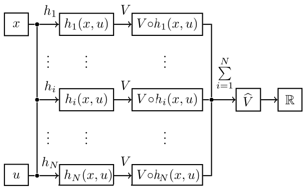
Remark 4. Unlike CISS-LFs, the GISS-LFs explicitly incorporate input-dependent terms through \(h_i(x,u)\), thereby providing greater flexibility in the selection of Lyapunov candidates for the ISS analysis. In the special case where \(h_i(x,u)\equiv x\) for all \(i\in\mathcal{I}\), the GISS-LF reduces to the classical one. The relationship between \(x,u,h_i,V,\widehat{V}\), and \(\mathbb{R}\) is illustrated in Fig. 1.
Remark 5. GISS-LFs have the following properties:
(i) Positive semidefiniteness. For a fixed \(u\), the functional \(\widehat{V}(x,u)\) may be degenerate at \(x\neq 0\), namely, \(\widehat{V} (x,u) =0\) at some \(x\neq 0\). Thus, a GISS-LF is positive semidefinite.
(ii) Coercivity w.r.t. \(x\). By virtue of condition ?? , the functional \(\widehat{V}(x,u)\) is coercive w.r.t. \(x\) in the sense that for any fixed \(u\), \[\begin{align} \|x\|_{X}\to +\infty ~~ \Rightarrow~~ \widehat{V}(x,u)\to +\infty. \end{align}\]
(iii) Non-coercivity w.r.t. \((x,u)\). Note that \(\widehat{V}(x,u)\) is non-coercive w.r.t. \((x,u)\) in the sense that \[\begin{align} \|x\|_{X}+ \|u\|_{\mathcal{U}}\to +\infty ~~\not\Rightarrow~~ \widehat{V}(x,u)\to +\infty. \end{align}\]
In the sequel, we always assume that conditions (H1) and (H2) are satisfied.
A generalized ISS Lyapunov theorem was proved in [56].
The following result, which is a direct consequence of Theorem 2, is suited for ISS analysis of specific PDEs involving only first order time derivatives, in particular, parabolic equations and first order hyperbolic equations.
Corollary 1 ([56]). Suppose that there exist a continuous functionalal \(V:X\to\mathbb{R}_{\geq 0}\), functions \(\psi_1,\psi_2\in\mathcal{K}_{\infty}, \mu,\rho\in \mathcal{K}\), and positive constant \(\lambda_0>0\) such that
for any \(x\in X\), it holds that \[\begin{align} 0\leq &V(x)\leq \psi_1(\| x\|_X); \end{align}\]
for any \(x\in X\) and any \(z\in X\), it holds that \[\begin{align} \psi_2\left(\| x \|_X\right) \leq { V(x-z )+V(-x-z )}+ \mu\left( \|z \|_{X} \right); \end{align}\]
for any \(u\in \mathcal{U}\), there is \(z_u\in X\) satisfying \(\|z_u\|_{X} \leq \rho(\|u\|_{\mathcal{U}})\), such that the derivative of \(V(x- {z_u})+V(-x-{z_u})\) along the trajectory satisfies \[\begin{align} \dot{V}(x- {z_u})+\dot{V}(-x-{z_u}) \leq &-\lambda_0( V(x- {z_u})+V(-x-{z_u})).\label{Equ4610} \end{align}\qquad{(13)}\]
Then, \(V(x- {z_u})+V(-x-{z_u})\) is a GISS-LF and the control system \(\Sigma\) is ISS.
Furthermore, noting that \(\mathcal{U}:=PC(\mathbb{R}_{\geq 0};U)\) (see condition (H1)), we can prove the following result, which is more convenient for conducting ISS analysis of PDEs.
Proposition 2. Under the conditions of Corollary 1 with (iii) replaced by
- for any \(T\in\mathbb{R}_{>0}\) and \(u\in \mathcal{U}\), there is \(z_{u,T}\in X\) satisfying \[\|z_{u,T}\|_{X} \leq \rho\left(\sup_{t\in(0,T)}\|u(t)\|_{ {U}}\right),\] such that the derivative of \(V(x- {z_{u,T}})+V(-x-{z_{u,T}})\) along the trajectory satisfies for all \(t\in(0,T)\): \[\begin{align} \dot{V}(x- {z_{u,T}})+\dot{V}(-x-{z_{u,T}}) \leq &-\lambda_0( V(x- {z_{u,T}})+V(-x-{z_{u,T}})),\label{Equ461039} \end{align}\qquad{(14)}\]
the control system \(\Sigma\) is ISS, having the estimate for all \(t\in \mathbb{R}_{>0}\): \[\begin{align} \psi_2\left(\| \phi(t,x,u) \|_X\right)\leq &2 e^{-\lambda_0t}\psi_1(2\| x\|_X) + \gamma \left( \sup_{s\in(0,t)}\|u(s)\|_{{U} }\right) \label{Equ4611} \end{align}\qquad{(15)}\] with \(\gamma(\cdot):= 2\psi_1(2\rho(\cdot))+\mu(\rho(\cdot))\in \mathcal{K}_{\infty}\).
Let \(\widehat{V}(x):= V(x- {z_{u,T}})+V(-x-{z_{u,T}})\). Applying the comparison principle ([62]) to ?? and using condition (i), we deduce that \[\begin{align} \widehat{V}(\phi(T,x,u)) \leq & e^{-\lambda_0 T} \widehat{V}(x)\notag\\ \leq & e^{-\lambda_0 T}\left(\psi_1(\|x-z_{u,T}\|_X)+\psi_1(\|-x-z_{u,T}\|_X)\right) \\ \leq & 2 e^{-\lambda_0 T}\left(\psi_1(\|x \|_X+ \| z_{u,T}\|_X)\right)\\ \leq &2 e^{-\lambda_0 T}\left(\psi_1(2\|x \|_X) + \psi_1(2\| z_{u,T}\|_X)\right)\notag\\ \leq & 2 e^{-\lambda_0 T }\psi_1(2\|x \|_X) +2 \psi_1(2\| z_{u,T}\|_X). \end{align}\] Using condition (ii) and the assumption that \(\|z_{u,T}\|_{X} \leq \rho\left(\sup_{t\in(0,T)}\|u(t)\|_{ {U}}\right)\), we obtain \[\begin{align} \psi_2\left(\| \phi(T,x,u) \|_X\right) \leq& \widehat{V}(\phi(T,x,u)) + \varphi\left( \|z_{u,T} \|_{X} \right) \\ \leq &2 e^{-\lambda_0 T} \psi_1(2\|x \|_X) + 2\psi_1(2\| z_{u,T}\|_X) + \mu\left( \|z_{u,T} \|_{X} \right)\notag\\ \leq & 2 e^{-\lambda_0 T} \psi_1(2\|x \|_X) + 2 \psi_1\left(2\rho\left(\sup_{t\in(0,T)}\|u(t)\|_{ {U}}\right)\right) + \mu\left(\rho\left(\sup_{t\in(0,T)}\|u(t)\|_{ {U}}\right)\right), \end{align}\] which, along with the arbitrariness of \(T\), gives the desired result. \(\blacksquare\)
Remark 6. By virtue Proposition 2, we call \(\widehat{V}(x):=V(x- {z_{u,T}})+V(-x-{z_{u,T}})\) a GISS-LF for the control system \(\Sigma\) over the arbitrary time interval \((0,T)\). Moreover, when \(T\) is not emphasized, we simply call \(\widehat{V}(x)\) a GISS-LF for the control system \(\Sigma\).
It is worth noting that, due to the diversity and complexity of PDEs, constructing an explicit GISS-LF within a unified framework is extremely challenging, and such constructions often require a case-by-case treatment. Nevertheless, for the most representative classes of PDEs, in particular, parabolic equations, first order hyperbolic equations, and wave equations, GISS-LFs can be constructed in a relatively unified manner. For these PDEs, a key technique lies in the use of Stampacchia’s truncation to construct truncation functions and disturbance-dependent energy functionals \(V(h_i(x,u))\). The number of such energy functionals is determined by the number of state variables when the PDE is reformulated as an abstract system. Details of constructing GISS-LFs for these three classes of PDEs are provided in Sections 3, 4, and 5, respectively.
3 ISS analysis for \(N\)-D parabolic equations via GLM↩︎
In this section, we construct a GISS-LF for higher dimensional parabolic PDEs with different disturbances under nonlinear boundary conditions.
In the sequel, let \(N\geq 1\), and let \(\Omega\) be an open bounded domain in \(\mathbb{R}^N\) with smooth (when \(N>1\)) boundary denoted by \(\partial \Omega\). At each point \(y\in\partial \Omega\), the unit outward normal vector is denoted by \(\boldsymbol{\nu}(y)\). For a differentiable function \(h\) defined over \(\Omega\), \(\nabla h\) denotes the gradient of \(h\). The notation \(\operatorname{d}\!{S}\) denotes the area element of \(\partial \Omega\). The notation \(\mathscr{L}^N(\Omega)\) (or \(\mathscr{L}^{N-1}(\Gamma)\)) denotes the \(N\)- (or \((N-1)\)-) dimensional Lebesgue measure of \(\Omega\) (or a set of \(\Gamma\in \partial \Omega\)). The notation \(\Delta\) represents the standard Laplace operator. For \(T>0\), let \(Q_T:=\Omega\times(0,T)\) and \(Q_{\infty}:=\Omega\times\mathbb{R}_{>0}\).
We consider the following higher dimensional nonlinear parabolic equation with both distributed in-domain and mixed boundary disturbances: \[\label{parabolicPDE-d} \begin{align} w_t(y,t) =&\operatorname{div}\!\; (a (y,t)\nabla w(y,t) )-c(y,t) \phi(w (y,t)) -{h(y,t,w(y,t) )} \notag\\ & +f(y,t),(y,t)\in Q_{\infty},\\ w(y,t) =&d_1(y,t),(y,t)\in \Gamma_1\times \mathbb{R}_{>0},\\ a(y,t) \frac{\partial w(y,t)}{\partial \boldsymbol{\nu}} =&-\varphi(w(y,t)) +d_2(y,t),(y,t)\in \Gamma_2\times \mathbb{R}_{>0},\\ w(y,0)=&w_0(y),y\in\Omega, \end{align}\tag{1}\] where
\(\Gamma_1\) and \(\Gamma_2\) are smooth and disjoint boundary sets (\((N-1)\)-dimensional hypersurfaces) satisfying (see, e.g., Fig. 2) \[\begin{align} \Gamma_1\cup\Gamma_2=& \partial \Omega,\\ 0\leq \mathscr{L}^{N-1}(\Gamma_1)\leq &\mathscr{L}^{N-1}(\partial \Omega); \end{align}\]
\(a,c :\Omega\times\mathbb{R}_{> 0}\to {\mathbb{R}_{> 0}}\) are smooth functions satisfying \[\begin{align} a(y,t ) \geq a_0 ,\forall (y,t )\in\Omega\times\mathbb{R}_{> 0},\\ c(y,t ) \geq c_0 ,\forall (y,t )\in\Omega\times\mathbb{R}_{> 0}, \end{align}\] with positive constants \(a_0\) and \(c_0\);
\(\phi: \mathbb{R} \to\mathbb{R}\) is a smooth and strictly increasing function satisfying \[\tag{2} \begin{align} \phi(v)v\geq & 0, \forall v\in \mathbb{R} , \\ \phi(-v) \leq &-\phi(v),\forall v\in \mathbb{R}_{\geq 0} ,\tag{3}\\ \phi'(v)\geq& 1,\forall v\in \mathbb{R} ;\tag{4} \end{align}\]
\(h:\Omega\times\mathbb{R}_{> 0}\times\mathbb{R}\to\mathbb{R}\) is a smooth function satisfying \[\begin{align} h(y,t,v)v\geq 0,\forall (y,t,v)\in\Omega\times\mathbb{R}_{> 0}\times\mathbb{R} ;\label{condition-h} \end{align}\tag{5}\]
\(\varphi: \mathbb{R} \to\mathbb{R}\) is a smooth and strictly increasing function satisfying \[\tag{6} \begin{align} \varphi(v)v\geq &0,\forall v\in \mathbb{R} ,\tag{7}\\ \varphi(-v) \leq &-\varphi(v),\forall v\in \mathbb{R}_{\geq 0} ;\tag{8} \end{align}\]
\(f,d_1,d_2:\Omega\times\mathbb{R}_{\geq 0}\to \mathbb{R}\) are smooth functions, representing distributed in-domain and boundary disturbances, respectively;
\(w_0:\Omega \to \mathbb{R}\) is a smooth function, representing the initial data.
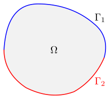
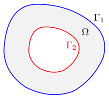
Figure 2: Illustration of a domain in \(\mathbb{R}^2\)..
We apply the technique of Stampacchia’s truncation to construct a GISS-LF. For any \(p\in(1,\infty)\), let \[\tag{9} \begin{align} g(s):=& \left\{\begin{aligned} & s^p,\;s\in \mathbb{R}_{\geq 0},\\ & 0,\;s\in \mathbb{R}_{< 0}, \end{aligned}\right.\tag{10}\\ G(s):=&\int_0^sg(\tau)\operatorname{d}\!{\tau} = \left\{\begin{align} & \frac{1}{p+1}s^{p+1},\;s\in \mathbb{R}_{\geq 0},\\ & 0,\;s\in \mathbb{R}_{< 0}.\end{align}\right. \end{align}\]
Note that \(g\) and \(G\) have the following properties, which will be extensively used in this paper:
\(G(s)=g(s)= 0\) for all \(s\in \mathbb{R}_{\leq 0}\);
\(G(s)=\frac{1}{p+1}g(s)s\) for all \(s\in \mathbb{R}\);
\(g'(s)\geq 0\) for all \(s\in \mathbb{R}\);
\(G(s )\leq G(s+\tau)+G(s-\tau)\) for all \(s,\tau\in \mathbb{R}\);
\(G(|s|+\tau )\leq G(s+\tau)+G(-s+\tau)\) for all \(s,\tau\in \mathbb{R}\);
\(G(s+\tau)\leq 2^p(G(s)+G(\tau))\) for all \(s,\tau\in \mathbb{R}\);
\(G(|s|)\leq 2^p (G(s+\tau-M)+G(s-\tau-M) +G(-s+\tau-M)+G(-s-\tau-M)) +2^pG(M)\) for all \(s,\tau,M\in\mathbb{R}\);
Young’s inequality: \[\begin{align} g(s)\tau\leq \varepsilon G(s)+\left(\frac{p}{\varepsilon}\right) ^{ p}G(\tau),\forall s,\tau\in \mathbb{R} , \varepsilon\in \mathbb{R}_{>0}. \end{align}\]
The proofs of properties (G1)-(G8) are provided in Appendix 8.
Since \(\phi\) and \(\varphi\) are strictly increasing, their inverses, denoted by \(\phi^{-1}\) and \(\varphi^{-1}\), respectively, exist. Moreover, \(\phi^{-1},\varphi^{-1}\in\mathcal{K}\). For any \(T>0\), let \[\begin{align} M:=&\phi^{-1}\left(\frac{1}{c_0} \|f\|_{\infty,T}\right) + \|d_1\|_{\infty,T} +\varphi^{-1}\left(\|d_2\|_{\infty,T}\right), \end{align}\] where, for notational simplicity, we denote \[\begin{align} \|f\|_{\infty,T}:=&\sup_{(y,t)\in Q_T}|f(y,t)| ,\\ \|d_1\|_{\infty,T}:=& \sup_{(y,t)\in \Gamma_1\times(0,T)}|d_1(y,t)| ,\\ \|d_2\|_{\infty,T}:=& \sup_{(y,t)\in \Gamma_2\times(0,T)}|d_2(y,t)|. \end{align}\] It is clear that \[\begin{align} \|f\|_{\infty,T} \leq& c_0\phi\left(M\right), \\ \|d_1\|_{\infty,T}\leq& M,\\ \|d_2\|_{\infty,T}\leq& \varphi(M). \end{align}\]
Let \[\begin{align} V(w):=& \int_{\Omega}G(w(y,t))\operatorname{d}\!{y}, \end{align}\] and \[\begin{align} \widehat{V}(w):= V (w -M) +V (-w -M).\label{GISS-LF-V} \end{align}\tag{11}\] Note that \(\widehat{V}(w)= 0\) for \(|w|\leq M\). Thus, \(\widehat{V}(w)\) is positive semidefinite.
For \(\widehat{V}(w)\) and system 1 , we have the following result.
Proposition 3. The following statements hold true:
For any \(p\in (1,\infty)\), the functional \(\widehat{V} (w)\) defined by 11 is a GISS-LF for system 1 over the arbitrary time interval \((0,T)\) and hence, system 1 is ISS in the \(L^{p+1}\)-norm.
Furthermore, system 1 is ISS in the \(L^{q}\)-norm for any \(q\in [2,\infty]\), having the estimate \[\begin{align} \| w(\cdot,T) \|_{L^{q}(\Omega)} \leq& 4 \| w_0 \|_{L^{q}(\Omega)}e^{-c_0 T}+8M,\forall T\in \mathbb{R}_{>0}.\label{q-estimate} \end{align}\qquad{(16)}\]
We employ Proposition 2 to prove this proposition.
First, it is clear that the conditions (i) and (ii) of Corollary 1 are fulfilled with (see [56]) \[\begin{align} \psi_1(s):=&\frac{1}{p+1} s^{p+1} ,\forall s\in \mathbb{R}_{\geq 0},\\ \psi_2(s):=&\frac{1}{ 2^{p}(p+1)}s^{p+1},\forall s\in \mathbb{R}_{\geq 0},\\ \mu(s):=&2s^{p+1},\forall s\in \mathbb{R}_{\geq 0}. \end{align}\] We shall verify the condition (iii’) of Proposition 2. Indeed, for any \(t\in(0,T)\), using the Green’s formula (see [63]), we deduce that \[\begin{align} \dot{V}(w-M) =& \frac{\diff~}{\operatorname{d}\!{t}} \int_{\Omega} G(w-M) \operatorname{d}\!{y} \notag\\ = & \int_{\Omega} g(w-M)w_t\operatorname{d}\!{y} \notag\\ = & \int_{\Omega} g(w-M)(\operatorname{div}\!\; (a w )-c \phi(w) -{h(y,t,w )}+f )\operatorname{d}\!{y}\notag\\ = & \int_{\Gamma_1} ag(w-M)\frac{\partial w}{\partial \boldsymbol{\nu}}\operatorname{d}\!{S}+ \int_{\Gamma_2} ag(w-M)\frac{\partial w}{\partial \boldsymbol{\nu}}\operatorname{d}\!{S} - \int_{\Omega}a g'(w-M)|\nabla w|^2 \operatorname{d}\!{y} \notag\\ &- \int_{\Omega} g(w-M) (c \phi(w)-f) \operatorname{d}\!{y} - \int_{\Omega} g(w-M) h(y,t,w) \operatorname{d}\!{y}.\label{parabolic-14} \end{align}\tag{12}\]
Using the boundary conditions, the definition of \(M\), 10 , and the monotonicity of \(\varphi\), we have \[\begin{align} g(w-M)=&0 \; \text{on}\; \Gamma_1\times (0,T) \end{align}\] and \[\begin{align} g(w-M)\frac{\partial w}{\partial \boldsymbol{\nu}} =&-g(w-M)(\varphi (w) -d_2)\notag\\ \leq& -g(w-M)\left( \varphi (w) -\|d_2\|_{\infty,T}\right)\notag\\ \leq& -g(w-M)\left( \varphi (w) -\varphi (M)\right)\notag\\ \leq& 0 \; \text{on}\; \Gamma_2\times (0,T). \end{align}\] The condition 5 ensures that \[\begin{align} h(y,t,v) \geq &0,\forall (y,t,v)\in\Omega\times(0,T)\times\mathbb{R}_{\geq 0} , \end{align}\] which, along with the definition \(g\), ensures that \[\begin{align} - g(w-M) h(y,t,w) \leq &0,\forall (y,t,w)\in\Omega\times(0,T)\times\mathbb{R} . \end{align}\] In addition, we deduce that \[\begin{align} -\int_{\Omega} g(w-M)(c\phi(w)- f)\operatorname{d}\!{y} \leq& -\int_{\Omega} g(w-M)\left(c\phi(w)- \|f\|_{\infty,T}\right)\operatorname{d}\!{y}\notag\\ \leq& -\int_{\Omega} g(w-M)\left(c\phi(w)- c_0\phi\left(M\right)\right)\operatorname{d}\!{y}\notag\\ \leq& -c_0\int_{\Omega} g(w-M)\left( \phi(w)- \phi\left(M\right)\right)\operatorname{d}\!{y}\notag\\ =& -c_0\int_{\Omega} g(w-M)\phi'(v)\left( w- M\right)\operatorname{d}\!{y}\notag\\ \leq & -c_0\int_{\Omega} g(w-M)(w- M)\operatorname{d}\!{y}\quad (\text{by}\;\eqref{condition-phi})\notag\\ =&-c_0(p+1)\int_{\Omega} G(w-M) \operatorname{d}\!{y}, \quad (\text{by}\;\boldsymbol{(G2)}) \end{align}\] where \(v\) is a function between \(w\) and \(M\).
Then, in view of (G3), for any \(t\in(0,T)\), we get \[\begin{align} \dot{V}(w-M) \leq & -c_0(p+1) \int_{\Omega} G(w-M) \operatorname{d}\!{y}\notag \\ =& -c_0(p+1) V(w-M).\label{parabolic-16} \end{align}\tag{13}\]
Now let \(\widetilde{w}:=-w\), which satisfies \[\label{parabolicPDE-d39} \begin{align} \widetilde{w}_t(y,t) =&\operatorname{div}\!\; (a (y,t)\nabla \widetilde{w}(y,t) ) +c(y,t) \phi(-\widetilde{w} (y,t)) +{h(y,t,-\widetilde{w}(y,t) )}\notag\\ & -f(y,t),(y,t)\in Q_{\infty},\\ \widetilde{w}(y,t) =&-d_1(y,t),(y,t)\in \Gamma_1\times \mathbb{R}_{>0},\\ a(y,t) \frac{\partial \widetilde{w}(y,t)}{\partial \boldsymbol{\nu}} =&\varphi(-\widetilde{w}(y,t)) -d_2(y,t),(y,t)\in \Gamma_2\times \mathbb{R}_{>0},\\ \widetilde{w}(y,0)=&-w_0(y),y\in\Omega, \end{align}\tag{14}\]
Note that \[\begin{align} g(\widetilde{w}-M)=&0 \; \text{on}\; \Gamma_1\times (0,T) \end{align}\] and \[\begin{align} g(\widetilde{w}-M)\frac{\partial \widetilde{w}}{\partial \boldsymbol{\nu}} =& g(\widetilde{w}-M)(\varphi (-\widetilde{w}) -d_2)\notag\\ \leq& g(\widetilde{w}-M)\left( \varphi (-\widetilde{w}) +\|d_2\|_{\infty,T}\right)\notag\\ \leq& g(\widetilde{w}-M)\left( \varphi (-\widetilde{w}) +\varphi (M)\right)\; \text{on}\; \Gamma_2\times (0,T). \end{align}\] Furthermore, in view of the nonnegativity of \(g\) and the degeneracy property (G1), the condition of \(\varphi\) (see 8 ) and the increasing monotonicity of \(\varphi\) imply that \[\begin{align} g(\widetilde{w}-M)\frac{\partial \widetilde{w}}{\partial \boldsymbol{\nu}} \leq& g(\widetilde{w}-M)\left( \varphi (-\widetilde{w}) +\varphi (M)\right) \notag\\ \leq & g(\widetilde{w}-M)\left( -\varphi (\widetilde{w}) +\varphi (M)\right)\\ \leq& 0 \; \text{on}\; \Gamma_2\times (0,T). \end{align}\]
Similarly, it holds that \[\begin{align} \int_{\Omega} g(\widetilde{w}-M)(c\phi(-\widetilde{w})+ f)\operatorname{d}\!{y} \leq& \int_{\Omega} g(\widetilde{w}-M)\left(-c\phi(\widetilde{w})+ c_0\phi\left(M\right)\right)\operatorname{d}\!{y}\notag\\ \leq& -c_0\int_{\Omega} g(\widetilde{w}-M)\left( \phi(\widetilde{w})- \phi\left(M\right)\right)\operatorname{d}\!{y}\notag\\ =& -c_0\int_{\Omega} g(\widetilde{w}-M)\phi'(v)\left( \widetilde{w}- M\right)\operatorname{d}\!{y}\notag\\ \leq &-c_0(p+1)\int_{\Omega} G(\widetilde{w}-M) \operatorname{d}\!{y},\forall t\in (0,T), \end{align}\] where \(v\) is a function between \(\widetilde{w}\) and \(M\).
In addition, due to the fact that \(h(y,t,v) \geq 0\) for all \((y,t,v)\in\Omega\times(0,T)\times\mathbb{R}_{\leq 0}\), we have \[\begin{align} g(\widetilde{w}-M) h(y,t,-\widetilde{w}) \leq &0,\forall (y,t,w)\in\Omega\times(0,T)\times\mathbb{R} . \end{align}\] Analogous to 13 , for any \(t\in(0,T)\), we have \[\begin{align} \dot{V}(\widetilde{w}-M) \leq & -c_0(p+1) \int_{\Omega} G(\widetilde{w}-M) \operatorname{d}\!{y} \notag\\ =& -c_0(p+1) V(\widetilde{w}-M), \label{parabolic-17} \end{align}\tag{15}\] which, along with 13 , indicates that the condition (iii’) of Proposition 2 is fulfilled with \(x:=w\), \(u:=(f,d_0,d_1)\), \(z_{u,T}:=M\), and \(\rho\left(\sup_{t\in(0,T)}\|u(t)\|_{ {U}}\right):=M\).
Applying Proposition 2 and Remark 6, we deduce that the functional \(\widehat{V} (w)\) defined by 11 is a GISS-LF for system 1 and hence, system 1 is ISS in the \(L^{p+1}\)-norm with arbitrary \(p\in (1,\infty)\).
Furthermore, we deduce by ?? that \[\begin{align} \psi_2\left( \| w(\cdot,T) \|_{L^{p+1}(\Omega)}\right)\leq &2 e^{-c_0(p+1)T}\psi_1\left(2\| w_0 \|_{L^{p+1}(\Omega)}\right) + 2\psi_1(2M)+\mu(M), \end{align}\] which implies that \[\begin{align} \| w(\cdot,T) \|_{L^{p+1}(\Omega)} \leq & \Big( 4 \| w_0 \|_{L^{p+1}(\Omega)} e^{-c_0 T} + 2M+ \left( p+1 \right)^{\frac{1}{p+1}}2M\Big)\notag\\ \leq& 4 \| w_0 \|_{L^{p+1}(\Omega)} e^{-c_0 T}+8M. \end{align}\] Thus, system 1 is ISS in the \(L^{p+1}\)-norm.
Furthermore, due to the arbitrariness of \(p\in(1,\infty)\), we conclude that system 1 is ISS in the \(L^{q}\)-norm for any \(q\in[2,\infty]\), having the estimate ?? . \(\blacksquare\)
Remark 7. Usually there is no need to verify each condition of Proposition 2 (or conditions (i)-(iii) in Definition 5) so as to obtain the ISS of a PDE. Indeed, one may directly compute \(\dot{\widehat{V}} (x,u)\) and using the Gronwall’s inequality to establish an explicit ISS estimate, where \(x\) and \(u\) denote the state and input of the considered PDE under an abstract form.
4 ISS analysis for \(1\)-D first order hyperbolic equations via GLM↩︎
In this section, we employ the GLM to establish ISS estimates for the following \(1\)-D hyperbolic equation: \[\label{first32hyperbolic32PDE} \begin{align} \rho_t(y,t)+\left(\lambda(W(t))\rho(y,t)\right)_y=&0, (y,t)\in (0,1)\times\mathbb{R}_{>0},\\ \rho(0,t)-k\rho(1,t)=&d(t),t\in \mathbb{R}_{>0},\\ \rho(y,0)=&\rho_0(y),y\in(0,1), \end{align}\tag{16}\] where \(\lambda\in C^1(\mathbb{R};\mathbb{R}_{>0})\), \(k\in(-1,1)\) is a constant, \(d,\rho_0\) are smooth functions, and \(W(t):=\int_0^1\rho(y,t)\operatorname{d}\!{y}\).
Equation 16 is commonly used to model semiconductor manufacturing systems; see, e.g., [64]–[66]. The key feature of this PDE is characterized by the velocity function \(\lambda\) depending on the total mass \(W(t)\).
We propose either one of the following assumptions on \(\lambda\):
\(\lambda(s)\geq \lambda_0\) for all \(s\in \mathbb{R}\), where \(\lambda_0\) is a positive constant;
\(\lambda(s)\geq \lambda(|s|)\) for all \(s\in \mathbb{R}\) and \(\lambda(s)\) is decreasing in \(s\in \mathbb{R}_{\geq 0}\).
Typical forms of \(\lambda(s)\) satisfying (A2) include \[\begin{align} \lambda(s):=Ae^{-s^2}+B,\forall s\in \mathbb{R}_{\geq 0} , \end{align}\] and \[\begin{align} \lambda(s):=\frac{A}{B+s},\forall s\in \mathbb{R}_{\geq 0} , \end{align}\] where \(A\) and \(B\) are positive constants.
For any \(p\in(1,\infty)\), let \(g\) and \(G\) be defined by 9 . For any \(T>0\), let \[\begin{align} M:= \frac{1}{1-|k|}\sup_{t\in (0,T)}|d (t)| = \left\{\begin{aligned} & \frac{1}{1-k}\sup_{t\in (0,T)}|d (t)|,\;k\in[0,1),\\ & \frac{1}{1+k}\sup_{t\in (0,T)}|d (t)|,\;k\in(-1,0). \end{aligned}\right. \end{align}\]
Let \[\begin{align} V(\rho):= \int_0^1e^{-r y}G(\rho(y,t))\operatorname{d}\!{y}, \end{align}\] where \(r\) is a positive constant satisfying \[\begin{align} 0< r\leq (p+1)\ln \frac{1}{|k|}.\label{condition-sigma} \end{align}\tag{17}\] Let \[\begin{align} \widehat{V}(\rho):= V (\rho -M) +V (-\rho -M).\label{GISS-LF-V-2} \end{align}\tag{18}\]
The first result for system 16 is regarded as a global ISS property.
Proposition 4. Under the assumption (A1), the following statements hold true.
(i) For any \(p\in (1,\infty)\) and \(r \in \mathbb{R}_{>0}\) satisfying 17 , the functional \(\widehat{V} (\rho)\) defined by 18 is a GISS-LF of system 16 and thus, system 16 is ISS in the \(L^{p+1}\)-norm. In particular, system 16 admits the following estimate: \[\begin{align} \|\rho(\cdot,t)\|_{L^{p+1}(0,1)} \leq & 2 e^{\frac{r}{p+1}}\|\rho_0 \|_{L^{p+1}(0,1)} e^{-\frac{r \lambda_0}{p+1} t} + 2 \sup_{s\in(0,t)} |d (s)| ,\forall t\in \mathbb{R}_{>0}.\label{PDE2-ISS-1} \end{align}\qquad{(17)}\]
(ii) Furthermore, for any \(q\in[2,\infty]\), system 16 is ISS in the \(L^{q}\)-norm and admits the following estimate: \[\begin{align} \|\rho(\cdot,t)\|_{L^{q}(0,1)} \leq & \frac{ 2 }{|k|} \|\rho_0 \|_{L^{q}(0,1)} |k|^{\frac{\lambda_0 t}{2}} +\frac{2}{1-|k|}\sup_{s\in (0,t)}|d (s)| ,\forall t\in \mathbb{R}_{>0}. \label{PDE2-ISS-2} \end{align}\qquad{(18)}\]
Remark 8. Note that \(|k|^{\frac{\lambda_0 t}{2}}=e^{-k_0t}\) with \(k_0:=\frac{\lambda_0}{2}\ln \frac{1}{|k|}>0\). Thus, similarly to ?? , estimate ?? also yields the exponential ISS for system 16 .
Using the GLM, we may establish local ISS estimates for system 16 with a general \(\lambda\).
Proposition 5. Under the assumption (A2), the following statements hold true.
(i) For any \(p\in (1,\infty)\) and \(r \in \mathbb{R}_{>0}\) satisfying 17 , system 16 is LISS in the \(L^{p+1}\)-norm, having the following estimate: \[\begin{align} \|\rho(\cdot,t)\|_{L^{p+1}(0,1)} \leq & 2 e^{\frac{r}{p+1}}\|\rho_0 \|_{L^{p+1}(0,1)} e^{-\frac{r \Lambda_0}{p+1} t} + 2 \sup_{s\in (0,t)}|d (s)| ,\forall t\in \mathbb{R}_{>0}, \end{align}\] provided that \[\begin{align} \|\rho_0 \|_{L^{p+1}(0,1)} + \sup_{t\in \mathbb{R}_{\geq 0}}|d (t)|\leq R_0\label{PDE2-31} \end{align}\qquad{(19)}\] with some positive constant \(R_0\), where \[\begin{align} \Lambda_0:= \lambda\left( 2R_0\max\left\{\frac{ 1 }{|k|}, \frac{ 1 }{1-|k|} \right\}\right)>0.\label{Lambda} \end{align}\qquad{(20)}\]
(ii) Furthermore, for any \(q\in[2,\infty]\), system 16 is LISS in the \(L^{q}\)-norm, having the following estimate: \[\begin{align} \|\rho(\cdot,t)\|_{L^{q}(0,1)} \leq & \frac{ 2 }{|k|} \|\rho_0 \|_{L^{q}(0,1)} |k|^{\frac{\Lambda_0 t}{2}} +\frac{2}{1-|k|}\sup_{s\in (0,t)}|d (s)| ,\forall t\in \mathbb{R}_{>0}, \end{align}\] provided that \[\begin{align} \|\rho_0 \|_{L^{q}(0,1)} + \sup_{t\in \mathbb{R}_{\geq 0}}|d (t)|\leq R_0 \end{align}\] with some positive constant \(R_0\), where \(\Lambda_0\) is the same as in ?? .
Now, we employ the GLM to prove Proposition 4 and Proposition 5, respectively.
We proceed the proof with three steps.
Step 1: We show that the functional \(\widehat{V} (\rho)\) defined by 18 is a GISS-LF for system 16 .
First, analogous to [56], it is direct to verify that the conditions (i) and (ii) of Corollary 1 are fulfilled. Next, for any \(t\in(0,T)\), we claim that \[\begin{align} \dot{\widehat{V}}(\rho) \leq& -r \lambda(W)\widehat{V}(\rho) \tag{19}\\ \leq& -r \lambda_0\widehat{V}(\rho) \forall t\in (0,T), \tag{20} \end{align}\] which, along with the conditions (i) and (ii) of Corollary 1, ensures that \(\widehat{V} (\rho)\) is a GISS-LF.
Now we prove 20 . Indeed, for any \(t\in(0,T)\), using integrating by parts, we obtain \[\begin{align} \dot{V}(\rho-M) =&\int_0^1e^{-r y}g(\rho-M)\rho_t\operatorname{d}\!{y}\notag\\ = &-\int_0^1e^{-r y}g(\rho-M) \left(\lambda(W)\rho(y,t)\right)_y \operatorname{d}\!{y}\notag\\ =&-\lambda(W)\int_0^1e^{-r y}\left(G(\rho-M) \right)_y \operatorname{d}\!{y}\notag\\ =&-\lambda(W)\left[e^{-r y}G(\rho-M)\right]_{y=0}^{y=1} -r \lambda(W)\int_0^1e^{-r y} G(\rho-M) \operatorname{d}\!{y}\notag\\ =&-\lambda(W)\left(e^{-r}G(\rho(1,t)-M)- G(\rho(0,t)-M)\right) -r \lambda(W)V(\rho-M)\notag\\ =&- \lambda(W) e^{-r}G(\rho(1,t)-M) +\lambda(W)G(k\rho(1,t)-M+d(t)) -r \lambda(W)V(\rho-M).\label{PDE2-V1} \end{align}\tag{21}\]
Analogously, we have \[\begin{align} \dot{V}(-\rho-M) =&- \lambda(W) e^{-r}G(-\rho(1,t)-M) +\lambda(W)G(-k\rho(1,t)-M-d(t)) \notag\\ &-r \lambda(W)V(-\rho-M), \forall t\in (0,T).\label{PDE2-V2} \end{align}\tag{22}\] Combining 21 and 22 , we have \[\begin{align} \dot{\widehat{V}}(\rho) \leq & \lambda(W) G(k\rho(1,t)-M+d(t)) +\lambda(W)G(-k\rho(1,t)-M-d(t)) - \lambda(W) e^{-r} G(\rho(1,t)-M) \notag\\ &- \lambda(W) e^{-r} G(-\rho(1,t)-M) -r \lambda(W)\widehat{V}(\rho),\forall t\in (0,T).\label{PDE2-hatV} \end{align}\tag{23}\]
Now we prove 20 in two cases: \(k\in[0,1)\) and \(k\in(-1,0)\).
Case 1: \(k\in[0,1)\). Note that \(G\) has the following property: \[\begin{align} \label{G-m} G(ms) = m^{p+1}G(s),\;\forall m\in\mathbb{R}_{\geq 0}, s\in\mathbb{R}. \end{align}\tag{24}\] Using the definition of \(M\), the monotonicity of \(G\), and 24 , we have \[\begin{align} G(k\rho(1,t)-M+d(t)) \leq & G(k\rho(1,t)-M+|d(t)|)\notag\\ \leq & G(k\rho(1,t)-M+(1-k)M) \notag\\ = &G( k(\rho(1,t)- M) )\notag\\ =&k^{p+1}G (\rho(1,t)- M),\forall t\in (0,T),\label{PDE2-34} \end{align}\tag{25}\] and \[\begin{align} G(-k\rho(1,t)-M-d(t)) \leq & G(-k\rho(1,t)-M+|d(t)|)\notag\\ \leq & G(-k\rho(1,t)-M+(1-k)M) \notag\\ = & G(k(-\rho(1,t) - M)) \notag\\ = &k^{p+1} G(-\rho(1,t) - M) ,\forall t\in (0,T).\label{PDE2-35} \end{align}\tag{26}\]
Putting 25 and 26 into 23 , we get \[\begin{align} \dot{\widehat{V}}(\rho) \leq & \lambda(W) \left(k^{p+1}-e^{-r}\right)G( \rho(1,t)-M) +\lambda(W) \left(k^{p+1}-e^{-r}\right)G( -\rho(1,t)-M) \notag\\ & -r \lambda(W)\widehat{V}(\rho),\forall t\in (0,T), \forall t\in (0,T).\label{PDE2-hatV39} \end{align}\tag{27}\] Note that the choice of \(r\) (see 17 ) implies that \[\begin{align} k^{p+1}- e^{-r}\leq 0 . \end{align}\] Then, 27 leads to 20 .
Case 2: \(k\in(-1,0)\). Analogous in Case 1, using the definition of \(M\), the monotonicity of \(G\), and 24 , we have \[\begin{align} G(k\rho(1,t)-M+d(t)) \leq & G(k\rho(1,t)-M+(1-|k|)M) \notag\\ = &G( k(\rho(1,t)+ M) )\notag\\ =&(-k)^{p+1}G (-\rho(1,t)- M),\forall t\in (0,T),\label{PDE2-3439} \end{align}\tag{28}\] and \[\begin{align} G(-k\rho(1,t)-M-d(t)) \leq & G(-k\rho(1,t)-M+(1-|k|)M) \notag\\ = & G(k(-\rho(1,t) + M)) \notag\\ = &(-k)^{p+1} G( \rho(1,t) - M) ,\forall t\in (0,T).\label{PDE2-3539} \end{align}\tag{29}\]
Putting 28 and 29 into 23 , we get \[\begin{align} \dot{\widehat{V}}(\rho) \leq & \lambda(W) \left((-k)^{p+1}-e^{-r}\right)G( \rho(1,t)-M) +\lambda(W) \left((-k)^{p+1}-e^{-r}\right)G( -\rho(1,t)-M) \notag\\ & -r \lambda(W)\widehat{V}(\rho),\forall t\in (0,T), \forall t\in (0,T).\label{PDE2-hatV393939} \end{align}\tag{30}\] Note that the choice of \(r\) (see 17 ) implies that \[\begin{align} (-k)^{p+1}=|k|^{p+1}\leq e^{-r} . \end{align}\] Then, 30 leads to 20 . We conclude that 20 holds true for all \(k\in(-,1,1)\).
Step 2: We prove the ISS estimate ?? . Indeed, applying the Gronwall’s inequality to 20 , we obtain \[\begin{align} {\widehat{V}}( \rho(y,T) ) \leq& e^{-r \lambda_0 T}\widehat{V}(\rho_0(y)).\notag \end{align}\] Therefore, using (G6) and (G5), we have \[\begin{align} \frac{1}{p+1}\int_0^1|\rho(y,T)|^{p+1}\operatorname{d}\!{y} = & \int_0^1G\left(|\rho(y,T)|\right)\operatorname{d}\!{y}\notag\\ \leq &2^{p}\int_0^1G\left(|\rho(y,T)|-M \right)\operatorname{d}\!{y}+2^{p}G(M)\notag\\ = &2^{p}\int_0^1\left(G\left( \rho(y,T)-M \right)+G\left(- \rho(y,T)-M \right)\right)\operatorname{d}\!{y} +2^{p}G(M)\notag\\ \leq &2^{p}e^{r}\left(V\left( \rho(y,T)-M \right)+ V\left( -\rho(y,T)-M \right)\right)+2^{p}G(M)\notag\\ =&2^{p}e^{r}{\widehat{V}}( \rho(y,T) )+2^{p}G(M)\notag\\ \leq &2^{p}e^{r}e^{-r \lambda_0 T}\widehat{V}(\rho_0(y))+2^{p}G(M)\notag\\ =&2^{p} e^{r} e^{-r \lambda_0 T}\int_0^1e^{-r y} \left(G(\rho_0(y)-M)+G(-\rho_0(y)-M) \right) \operatorname{d}\!{y} +2^{p}G(M)\notag\\ = &2^{p}e^{r}e^{-r \lambda_0 T} \int_0^1e^{-r y} G(|\rho_0(y)|-M) \operatorname{d}\!{y} +2^{p}G(M)\notag\\ \leq &2^{p}e^{r}e^{-r \lambda_0 T} \int_0^1 G(|\rho_0(y)| ) \operatorname{d}\!{y} +2^{p}G(M)\notag\\ =& \frac{2^{p}e^{r}}{p+1}e^{-r \lambda_0 T} \int_0^1|\rho_0(y)|^{p+1}\operatorname{d}\!{y} +\frac{2^{p}}{p+1}M^{p+1}, \label{PDE2-26} \end{align}\tag{31}\] which implies that \[\begin{align} \|\rho(\cdot,T)\|_{L^{p+1}(0,1)} \leq & 2^{\frac{p}{p+1}}e^{\frac{r}{p+1}} e^{-\frac{r \lambda_0}{p+1} T}\|\rho_0 \|_{L^{p+1}(0,1)} + 2^{\frac{p}{p+1}} M,\forall T\in \mathbb{R}_{>0}. \label{PDE2-27} \end{align}\tag{32}\] Therefore, the ISS estimate ?? holds true.
Step 3: We prove the ISS estimate ?? . Now let \(r\) satisfy \[\begin{align} 0<-\frac{1}{2}(p+1)\ln |k|\leq r\leq -(p+1)\ln |k|,\label{condition-sigma39} \end{align}\tag{33}\] which ensures that \[\begin{align} e^{\frac{r}{p+1}} \leq \frac{1}{|k|} \;\;\text{and}\;\; e^{-\frac{r}{p+1}} \leq |k|^{\frac{1}{2}} . \end{align}\] For any \(T\in \mathbb{R}_{>0}\), it follows from 32 that \[\begin{align} \|\rho(\cdot,T)\|_{L^{p+1}(0,1)} \leq & \frac{ 2 }{|k|} |k|^{\frac{\lambda_0 T}{2}} \|\rho_0 \|_{L^{p+1}(0,1)} + 2 M .\label{PDE2-28} \end{align}\tag{34}\] Therefore, the ISS estimate ?? holds true for any \(q:=p+1 \in (2,\infty)\).
letting \(p\to 1\) and \(p\to \infty\) in 34 yields that the ISS estimate ?? holds for \(q=2\) and \(q=\infty\), respectively. \(\blacksquare\)
For any \(T\in \mathbb{R}_{>0}\), applying the Gronwall’s inequality to 19 , we obtain \[\begin{align} {\widehat{V}}( \rho(y,T) ) \leq& e^{-r \int_0^T\lambda(W(t))\operatorname{d}\!{t}}\widehat{V}(\rho_0(y)).\label{hatV-W40t41} \end{align}\tag{35}\] It follows that \[\begin{align} {\widehat{V}}( \rho(y,T) ) \leq& \widehat{V}(\rho_0(y)), \end{align}\] which, along with similar derivations for 31 , 32 , and 34 (by setting \(\lambda_0=0\) in 31 , 32 , and 34 ), leads to \[\begin{align} \|\rho(\cdot,T)\|_{L^{p+1}(0,1)} \leq & \frac{ 2 }{|k|} \|\rho_0 \|_{L^{p+1}(0,1)} + 2 M . \end{align}\] It follows that \[\begin{align} |W(T)| \leq & \|\rho(\cdot,T)\|_{L^{p+1}(0,1)}\notag\\ \leq & \frac{ 2 }{|k|} \|\rho_0 \|_{L^{p+1}(0,1)} + \frac{2}{1-|k|}\sup_{t\in (0,T)}|d (t)|. \end{align}\] Thus, for \(\rho_0\) and \(d\) satisfying ?? , i.e., \[\begin{align} \|\rho_0 \|_{L^{p+1}(0,1)} + \sup_{t\in \mathbb{R}_{\geq 0}}|d (t)|\leq R_0 \end{align}\] with some positive constant \(R_0\), it holds that \[\begin{align} |W(T)| \leq & 2R_0\max\left\{\frac{ 1 }{|k|}, \frac{ 1 }{1-|k|} \right\} . \end{align}\] According to the assumption (A2), we have \[\begin{align} \lambda(W(T))\geq &\lambda(|W(T)|)\notag\\ \geq & \Lambda_0:= \lambda\left( 2R_0\max\left\{\frac{ 1 }{|k|}, \frac{ 1 }{1-|k|} \right\}\right). \end{align}\] Then, 35 becomes \[\begin{align} {\widehat{V}}( \rho(y,T) ) \leq& e^{-r \int_0^T\lambda(W(t))\operatorname{d}\!{t}}\widehat{V}(\rho_0(y)) \\ \leq & e^{-r \int_0^T\Lambda_0 \operatorname{d}\!{t}}\widehat{V}(\rho_0(y))\notag \\ =& e^{-r \Lambda_0 T}\widehat{V}(\rho_0(y)).\notag \end{align}\] The remaining part of the proof is exactly the same as the proof of Proposition 4. \(\blacksquare\)
5 ISS analysis for \(1\)-D wave equations via GLM↩︎
In this section, we employ the GLM to establish ISS estimates for the following \(1\)-D wave equation with boundary velocity damping: \[\label{second32hyperbolic32PDE} \begin{align} w_{tt}(y,t)=&c^2w_{yy}(y,t) +f(y,t), (y,t)\in (0,1)\times\mathbb{R}_{>0},\\ w(0,t)=&0,t\in \mathbb{R}_{>0},\\ w_y(1,t)=&-kw_t(1,t)+d(t),t\in \mathbb{R}_{>0},\\ w(y,0)=&w_0(y), y\in(0,1),\\ w_t(y,0)=&\phi_0(y), y\in(0,1), \end{align}\tag{36}\] where \(c\) and \(k\) are positive constants satisfying \[\begin{align} ck=1, \end{align}\] \(f,d:\mathbb{R}_{>0}\to \mathbb{R}\) are smooth functions, representing distributed in-domain and boundary disturbances, respectively, and \(w_0\) and \(\phi_0\) are smooth functions, representing the initial data.
It is worth mentioning that the CLM has been employed to establish the ISS in the norm of Hilbert spaces for the \(1\)-D wave equation with different dampings; see [67], [68]. In this paper, we show how to use the GLM to establish the ISS in the norm of Banach spaces for the wave equation with boundary velocity damping.
For any \(p\in(1,\infty)\), let \(g\) and \(G\) be defined by 9 . For any \(T>0\), let \[\begin{align} M:= \frac{1}{c}\sup_{t\in (0,T)}|d (t)|. \end{align}\]
For \(v\in C(\mathbb{R}_{>0};L^{p+1}(0,1))\), define \[\begin{align} V_1 (v):= &\int_0^1e^{r y}G(v(y,t))\operatorname{d}\!{y},\\ V_2(v):=&\int_0^1e^{-r y}G(v(y,t))\operatorname{d}\!{y}, \end{align}\] where \(r\) is a positive constant. Let \[\begin{align} \widehat{V}(w):= &V_1 (w_t+cw_y -M) +V_1 (-w_t-cw_y -M) +V_2 (w_t-cw_y -M) +V_2 (-w_t+cw_y -M). \end{align}\]
Proposition 6. The following statements hold true.
For any \(p\in(1,\infty)\) and \(r\in \mathbb{R}_{>0}\), \(\widehat{V}(w)\) is a GISS-LF for system 36 and thus, system 36 is ISS in the \(L^{p+1}\)-norm. Furthermore, for any \(q\in[2,\infty)\), system 36 is ISS in the \(L^{q}\)-norm, having the estimate: \[\begin{align} \|w_t(\cdot,T)\|_{L^{q}(0,1)}+\|w_y(\cdot,T)\|_{L^{q}(0,1)} \leq& 2^{\frac{q-1}{q}} \bigg[ 2^{\frac{q+1}{q} } e^{\frac{2r-(cr-\varepsilon)T}{q}}\left(\|\phi_0\|_{L^{q}(0,1)}+\|w_{0y}\|_{L^{q}(0,1)}\right)\notag\\ &+ \left(\frac{q-1}{\varepsilon}\right) ^{ \frac{q-1}{q}} \left(\frac{8e^{2r}}{cr-\varepsilon}\right)^{\frac{1}{q}} \sup_{(y,t)\in (0,1)\times (0,T)}|f(y,t)| \notag\\ & + \frac{2}{c}\sup_{t\in (0,T)}|d (t)| \bigg],\forall T\in \mathbb{R}_{>0},\label{PDE3-ISS-1} \end{align}\qquad{(21)}\] where \(r,\varepsilon\in\mathbb{R}_{>0}\) are arbitrary constants satisfying \(cr-\varepsilon>0\).
For any \(q\in[2,\infty]\), system 36 is ISS in the \(L^{q}\)-norm, having the estimate: \[\begin{align} \|w_t(\cdot,t)\|_{L^{q}(0,1)}+\|w_y(\cdot,t)\|_{L^{q}(0,1)} \leq& 8 e^{\frac{4m}{c} }e^{-\frac{1}{2}mt}\left(\|\phi_0\|_{L^{q}(0,1)} +\|w_{0y}\|_{L^{q}(0,1)}\right) \notag\\ &+ \frac{16}{m } e^{\frac{4m}{c} } \sup_{(y,s)\in (0,1)\times (0,t)}|f(y,s)|\notag\\ &+ \frac{4}{c}\sup_{s\in (0,t)}|d (s)| ,\forall t\in \mathbb{R}_{>0},\label{PDE3-ISS-2} \end{align}\qquad{(22)}\] where \(m \in\mathbb{R}_{>0}\) is an arbitrary constant.
Remark 9. Due to arbitrariness of \(r\) in ?? (or \(m\) in ?? ), the disturbance-free system is superstable and hence, finite-time stable, namely, the energy decays to zero in finite time; see [69], [70].
We proceed the proof in four steps.
Step 1: Calculate the derivative of \(\widehat{V}\).
Indeed, for any \(t\in(0,T)\), using integrating by parts, we obtain \[\begin{align} \dot{V}_1(w_t+cw_y -M) =&\int_0^1e^{ r y}g(w_t+cw_y -M)(w_{tt}+cw_{yt})\operatorname{d}\!{y}\notag\\ =&\int_0^1e^{ r y}g(w_t+cw_y -M)( c^2w_{yy}+f+cw_{yt})\operatorname{d}\!{y}\notag\\ =&c\int_0^1e^{ r y}g(w_t+cw_y -M)( w_{t}+c w_{y })_y\operatorname{d}\!{y}+\int_0^1e^{ r y}g(w_t+cw_y -M) f \operatorname{d}\!{y}\notag\\ =&c\int_0^1e^{ r y}\left(G(w_t+cw_y -M)\right)_y\operatorname{d}\!{y} +\int_0^1e^{ r y}g(w_t+cw_y -M) f \operatorname{d}\!{y}\notag\\ =&c \left[e^{ r y}G(w_t+cw_y -M)\right]_{y=0}^{y=1} -cr{V}_1(w_t+cw_y -M)\notag\\ & +\int_0^1e^{ r y}g(w_t+cw_y -M) f \operatorname{d}\!{y}.\label{PDE3-53} \end{align}\tag{37}\]
Using the Young’s inequality (see (G8)), we have \[\begin{align} \int_0^1e^{ r y}g(w_t+cw_y -M) f \operatorname{d}\!{y} \leq &\varepsilon \int_0^1e^{ r y}G(w_t+cw_y -M) \operatorname{d}\!{y}\notag\\ & +\left(\frac{p}{\varepsilon}\right) ^{ p} \int_0^1e^{ r y}G(|f|) \operatorname{d}\!{y},\forall \varepsilon\in \mathbb{R}_{>0}.\label{PDE3-54} \end{align}\tag{38}\] We infer from 37 and 38 that \[\begin{align} \dot{V}_1(w_t+cw_y -M) \leq & -(cr-\varepsilon) {V}_1(w_t+cw_y -M)+\left(\frac{p}{\varepsilon}\right) ^{ p} V_1(|f|) \notag\\ & + c \left[e^{ r y}G(w_t+cw_y -M)\right]_{y=0}^{y=1} ,\forall t\in(0,T). \label{PDE3-55} \end{align}\tag{39}\] Analogously, we deduce that \[\begin{align} \dot{V}_1(-w_t-cw_y -M) \leq & -(cr-\varepsilon) {V}_1(-w_t-cw_y -M)+\left(\frac{p}{\varepsilon}\right) ^{ p} V_1(|f|)\notag\\ & + c \left[e^{ r y}G(-w_t-cw_y -M)\right]_{y=0}^{y=1} ,\forall t\in(0,T), \label{PDE3-56} \end{align}\tag{40}\] \[\begin{align} \dot{V}_2(w_t-cw_y -M) \leq & -(cr-\varepsilon) {V}_2(w_t-cw_y -M)+\left(\frac{p}{\varepsilon}\right) ^{ p} V_2(|f|) \notag\\ &- c \left[e^{ -r y}G(w_t-cw_y -M)\right]_{y=0}^{y=1} ,\forall t\in(0,T), \label{PDE3-57} \end{align}\tag{41}\] and \[\begin{align} \dot{V}_2(-w_t+cw_y -M) \leq & -(cr-\varepsilon) {V}_2(-w_t+cw_y -M)+\left(\frac{p}{\varepsilon}\right) ^{ p} V_2(|f|)\notag\\ & - c \left[e^{ -r y}G(-w_t+cw_y -M)\right]_{y=0}^{y=1} ,\forall t\in(0,T), \label{PDE3-58} \end{align}\tag{42}\] where \(\varepsilon\) keeps the same value and satisfies \[\begin{align} cr-\varepsilon>0. \end{align}\]
Combining 39 , 40 , 41 , and 42 , we obtain \[\begin{align} \dot{\widehat{V}}(w) \leq & -(cr-\varepsilon) \widehat{V} (w)+2\left(\frac{p}{\varepsilon}\right) ^{ p} \left( V_1(|f|)+V_2(|f|)\right) +cB(t) \notag\\ \leq & -(cr-\varepsilon) \widehat{V} (w)+4\left(\frac{p}{\varepsilon}\right) ^{ p} V_1(|f|) +cB(t), \forall t\in(0,T), \label{PDE3-59} \end{align}\tag{43}\] where \[\begin{align} B(t):=& \left[e^{ r y}G(w_t+cw_y -M)\right]_{y=0}^{y=1} + \left[e^{ r y}G(-w_t-cw_y -M)\right]_{y=0}^{y=1} - \left[e^{ -r y}G(w_t-cw_y -M)\right]_{y=0}^{y=1} \notag\\ &- \left[e^{ -r y}G(-w_t+cw_y -M)\right]_{y=0}^{y=1} . \end{align}\]
Step 2: Handle the boundary term \(B(t)\).
Using the boundary conditions, the fact that \(ck=1\), and the monotonicity of \(G\), we have \[\begin{align} B(t) =& e^{ r }G(w_t(1,t)+cw_y(1,t) -M) - G(w_t(0,t)+cw_y(0,t) -M) \notag\\ &+e^{ r }G(-w_t(1,t)-cw_y(1,t) -M) - G(-w_t(0,t)-cw_y(0,t) -M)\notag\\ & - e^{ -r }G(w_t(1,t)-cw_y(1,t) -M) + G(w_t(0,t)-cw_y(0,t) -M) \notag\\ &- e^{ -r }G(-w_t(1,t)+cw_y(1,t) -M) +G(-w_t(0,t)+cw_y(0,t) -M)\notag\\ =& e^{ r }G(w_t(1,t)+c(-kw_t(1,t)+d(t)) -M) - G(w_t(0,t)+cw_y(0,t) -M)\notag\\ & +e^{ r }G(-w_t(1,t)-c(-kw_t(1,t)+d(t)) -M) - G(-cw_y(0,t) -M)\notag\\ &- e^{ -r }G(w_t(1,t)-c(-kw_t(1,t)+d(t)) -M) + G(-cw_y(0,t) -M) \notag\\ &- e^{ -r }G(-w_t(1,t)+c(-kw_t(1,t)+d(t)) -M) +G(cw_y(0,t) -M)\notag\\ =& e^{ r }G( c d(t) -M) - G(cw_y(0,t) -M) +e^{ r }G(-c d(t) -M) - G(-cw_y(0,t) -M) \notag\\ &+ G(-cw_y(0,t) -M) - e^{ -r }G(-2w_t(1,t)+c d(t) -M) +G(cw_y(0,t) -M)\notag\\ =& e^{ r }G( c d(t) -M) +e^{ r }G(-c d(t) -M) - e^{ -r }G(2w_t(1,t)-c d(t) -M) \notag\\ & - e^{ -r }G(-2w_t(1,t)+c d(t) -M) \notag\\ \leq & e^{ r }G( c d(t) -M) +e^{ r }G(-c d(t) -M) \notag\\ \leq & e^{ r }G( c |d(t)| -M) +e^{ r }G(|-c d(t)| -M) \notag\\ \leq & e^{ r }G( M -M) +e^{ r }G(M -M) \notag\\ =& 0,\forall t\in (0,T). \end{align}\]
Step 3: Establish the ISS estimate ?? .
Since \(B(t)\leq 0\) for all \(t\in (0,T)\), we deduce from 43 that \[\begin{align} \dot{\widehat{V}}(w) \leq & -(cr-\varepsilon) \widehat{V} (w) +4\left(\frac{p}{\varepsilon}\right) ^{ p} V_1(|f|) \notag\\ \leq & -(cr-\varepsilon) \widehat{V} (w) +4e^{ r} \left(\frac{p}{\varepsilon}\right) ^{ p}\frac{1}{p+1}\|f\|_{\infty,T}^{p+1} , \forall t\in(0,T), \label{PDE3-61} \end{align}\tag{44}\] where, and in the sequel, \[\begin{align} \|f\|_{\infty,T}:=\sup_{(y,t)\in (0,1)\times (0,T)}|f(y,t)|. \end{align}\]
Applying the Gronwall’s inequality to 44 , we obtain \[\begin{align} \widehat{V} (w(y,T)) \leq & e^{-(cr-\varepsilon)T} \widehat{V} (w(y,0)) + \frac{4e^{ r}}{p+1}\left(\frac{p}{\varepsilon}\right) ^{ p}\|f\|_{\infty,T}^{p+1}\int_0^Te^{-(cr-\varepsilon)(T-t)} \operatorname{d}\!{t}\notag\\ \leq &e^{-(cr-\varepsilon)T} \widehat{V} (w(y,0)) +\frac{4e^{ r}}{p+1} \left(\frac{p}{\varepsilon}\right) ^{ p} \frac{1}{cr-\varepsilon} \|f\|_{\infty,T}^{p+1}. \label{PDE3-62} \end{align}\tag{45}\] Using the definition of \(\widehat{V}\), (G7), and (G6), we infer from 45 that \[\begin{align} &\frac{1}{p+1}\left(\|w_t(\cdot,T)\|^{p+1}_{L^{p+1}(0,1)}+\|w_y(\cdot,T)\|^{p+1}_{L^{p+1}(0,1)}\right) \notag\\ =& \int_0^1G(|w_t(y,T)|)\operatorname{d}\!{y}+\int_0^1G(|w_y(y,T)|)\operatorname{d}\!{y}\notag\\ \leq & e^r\widehat{V} (w(y,T))+2^{p}G(M)+e^r\widehat{V} (w(y,T))+2^{p}G(M)\notag\\ \leq &2 e^{r-(cr-\varepsilon)T} \widehat{V} (w(y,0)) +\frac{8e^{ 2r}}{p+1} \left(\frac{p}{\varepsilon}\right) ^{ p} \frac{1}{cr-\varepsilon} \|f\|_{\infty,T}^{p+1} +2^{p+1}G(M)\notag\\ = &2 e^{r-(cr-\varepsilon)T} V_1(|\phi_0(y)+cw_{0y}(y)|-M) +2 e^{r-(cr-\varepsilon)T} V_2(|\phi_0(y)+cw_{0y}(y)|-M) \notag\\ &+\frac{8e^{ 2r}}{p+1} \left(\frac{p}{\varepsilon}\right) ^{ p} \frac{1}{cr-\varepsilon} \|f\|_{\infty,T}^{p+1} +2^{p+1}G(M)\notag\\ \leq & 2 e^{r-(cr-\varepsilon)T} V_1(|\phi_0(y)+cw_{0y}(y)| ) +2 e^{r-(cr-\varepsilon)T} V_2(|\phi_0(y)+cw_{0y}(y)| ) \notag\\ &+\frac{8e^{ 2r}}{p+1} \left(\frac{p}{\varepsilon}\right) ^{ p} \frac{1}{cr-\varepsilon} \|f\|_{\infty,T}^{p+1} +2^{p+1}G(M)\notag\\ \leq & 2 e^{r-(cr-\varepsilon)T} 2^{p} ( V_1(|\phi_0(y)|)+V_1(|cw_{0y}(y)| ) ) +2 e^{r-(cr-\varepsilon)T} 2^{p} ( V_2(|\phi_0(y)|)+V_2(|cw_{0y}(y)| ) ) \notag\\ &+\frac{8e^{ 2r}}{p+1} \left(\frac{p}{\varepsilon}\right) ^{ p} \frac{1}{cr-\varepsilon} \|f\|_{\infty,T}^{p+1} +2^{p+1}G(M)\notag\\ \leq & 2^{p+2}e^{2r-(cr-\varepsilon)T} \int_0^1 G(|\phi_0(y)| )\operatorname{d}\!{y} + 2^{p+2}c^{p+1}e^{2r-(cr-\varepsilon)T}\int_0^1 G(|w_{0y}(y)| )\operatorname{d}\!{y} \notag\\ &+\frac{8e^{ 2r}}{p+1} \left(\frac{p}{\varepsilon}\right) ^{ p} \frac{1}{cr-\varepsilon} \|f\|_{\infty,T}^{p+1} +2^{p+1}G(M)\notag\\ =& \frac{2^{p+2}}{p+1}e^{2r-(cr-\varepsilon)T}\left(\|\phi_0\|^{p+1}_{L^{p+1}(0,1)}+\|w_{0y}\|^{p+1}_{L^{p+1}(0,1)}\right) +\frac{8e^{ 2r}}{p+1} \left(\frac{p}{\varepsilon}\right) ^{ p} \frac{1}{cr-\varepsilon} \|f\|_{\infty,T}^{p+1} \notag\\ &+\frac{2^{p+1}}{p+1}M^{p+1}, \end{align}\] which implies that system 36 is ISS in the \(L^{p+1}\)-norm, having the estimate \[\begin{align} \|w_t(\cdot,T)\|_{L^{p+1}(0,1)}+\|w_y(\cdot,T)\|_{L^{p+1}(0,1)} \leq& 2^{\frac{p}{p+1}} \bigg[ 2^{\frac{p+2}{p+1} } e^{\frac{2r-(cr-\varepsilon)T}{p+1}}\left(\|\phi_0\|_{L^{p+1}(0,1)}+\|w_{0y}\|_{L^{p+1}(0,1)}\right)\notag\\ &+ \left(\frac{p}{\varepsilon}\right) ^{ \frac{p}{p+1}} \left(\frac{8e^{2r}}{cr-\varepsilon}\right)^{\frac{1}{p+1}} \|f\|_{\infty,T} + 2M \bigg],\forall T\in \mathbb{R}_{>0}.\label{PDE3-ISS-139} \end{align}\tag{46}\]
In addition, due to the arbitrariness of \(p\), we conclude that ?? holds true for all \(q\in [2,\infty)\).
Step 4: Establish the ISS estimate ?? .
For any given \(m>0\), letting \(r=\frac{2m}{c}p\) and \(\varepsilon=mp\) in 46 yields \[\begin{align} &\|w_t(\cdot,T)\|_{L^{p+1}(0,1)}+\|w_y(\cdot,T)\|_{L^{p+1}(0,1)}\\ \leq& 2^{\frac{p}{p+1}} \bigg[ 2^{\frac{p+2}{p+1} } e^{\frac{4m}{c}\frac{p}{p+1}}e^{-\frac{p}{p+1}mT}\left(\|\phi_0\|_{L^{p+1}(0,1)}\right. \left. +\|w_{0y}\|_{L^{p+1}(0,1)}\right)\notag\\ &+ \left(\frac{1}{m}\right)^{\frac{p}{p+1}}\left( \frac{8}{mp}\right)^{\frac{1}{p+1}} e^{\frac{4m}{c}\frac{p}{p+1}} \|f\|_{\infty,T} + 2M \bigg] \notag\\ \leq & 2 \bigg[ 4 e^{\frac{4m}{c} }e^{-\frac{1}{2}mT}\left(\|\phi_0\|_{L^{p+1}(0,1)} +\|w_{0y}\|_{L^{p+1}(0,1)}\right) + \left(\frac{1}{m}\right)^{\frac{p}{p+1}}\left( \frac{8}{m}\right)^{\frac{1}{p+1}} e^{\frac{4m}{c} } \|f\|_{\infty,T} + 2M \bigg] \notag\\ = &8 e^{\frac{4m}{c} }e^{-\frac{1}{2}mT}\left(\|\phi_0\|_{L^{p+1}(0,1)} +\|w_{0y}\|_{L^{p+1}(0,1)}\right)+ \frac{16}{m} e^{\frac{4m}{c} } \|f\|_{\infty,T} + 4M ,\forall T\in \mathbb{R}_{>0}, \end{align}\] which, along with the arbitrariness of \(p>1\), implies ?? . \(\blacksquare\)
Remark 10. It is worth noting that when using the GLM for ISS analysis, handling each boundary term in \(B(t)\) independently would make it difficult to obtain effective estimates. Instead, as shown in Step 2, to eliminate the impact of boundary disturbances, all boundary terms in \(B(t)\) must be treated as a whole in a unified manner.
6 Conclusion↩︎
In this paper, within the framework of abstract control systems, we have revisited the concept of (classical) ISS-LF, the (classical) ISS-Lyapunov theorem, as well as the notion of GISS-LF and the GISS-Lyapunov theorem. A distinctive feature of the GISS-LF is its dependence on the external inputs, which generalizes the classical ISS-LF and provides greater flexibility for the ISS analysis of concrete PDEs. In particular, in the presence of Dirichlet boundary disturbances, the GISS-LF demonstrates superior efficiency than the classical ISS-LF. We refer to this approach of ISS analysis via the construction of GISS-LFs as the generalized Lyapunov method (GLM). To illustrate the general applicability of GLM, we have shown in detail how to construct GLFs for three representative examples, namely, an \(N\)-dimensional parabolic PDE, a first order hyperbolic PDE, and a wave equation with boundary damping, and based on which, established the corresponding ISS estimates in general \(L^q\) spaces. These examples cover the main features of parabolic, first order hyperbolic, and second order hyperbolic equations, providing a validation of the applicability of the GLM to different classes of PDEs. It is worth noting that, due to the diversity of PDEs, constructing a universally applicable GISS-LF in an explicit form for general PDEs remains an open problem. In future work, we will continue to focus on developing GISS-LFs tailored to a wider range of specific PDEs, explore the intrinsic connection between GISS-LF and controller design, particularly in the context of observer design and output feedback control.
7 Technical lemmas↩︎
Lemma 1 (Young’s inequality with \(\epsilon\), [63]). Let \(r,q\in(1, \infty)\) satisfy \(\frac{1}{r}+\frac{1}{q}=1\). It holds that \[\begin{align} ab\leq \epsilon a^r+C(\epsilon)b^q,\forall a,b\in \mathbb{R}_{\geq 0},\forall \epsilon\in \mathbb{R}_{>0}, \end{align}\] where \(C(\varepsilon):= (\epsilon r)^{-\frac{q}{r}} q^{-1}\).
Lemma 2 (Gronwall’s inequality, [63]). For \(T\in\mathbb{R}_{>0}\), let \(\phi\) and \(\psi\) be integrable functions on \([0,T]\), and \(\eta\) an absolutely continuous function on \([0,T]\). If \(\eta\) satisfies the differential inequality for all most every \(t\in [0,T]\): \[\begin{align} \eta'(t)\leq \phi (t)\eta(t)+\psi(t), \end{align}\] then, it holds that \[\begin{align} \eta(t)\leq e^{\int_{0}^t\phi(s)\text{d}s} \eta(0)+\int_{0}^t e^{ \int_{s}^t\phi(r)\text{d}r}\psi(s)\operatorname{d}\!{s} , \forall t\in [0,T]. \end{align}\]
8 Proofs of properties (G1)-(G8)****↩︎
Indeed, properties (G1)-(G3) can be directly verified via the definition of \(g\) and \(G\).
Using the increasing monotonicity of \(G\), i.e., (G3), we get \(G(s)\leq G(s+\tau)\) for \(\tau\geq 0\) and \(G(s)\leq G(s-\tau)\) for \(\tau\leq 0\), respectively. Thus, (G4) holds true.
Since \(G(|s|+\tau)= G(s+\tau)\) for \(s\geq 0\) and \(G(|s|+\tau)= G(-s+\tau)\) for \(s\leq 0\), we obtain (G5).
For (G6), it suffices to note that \((s+\tau)^{p+1}\leq 2^{p}(s^{p+1}+\tau^{p+1})\) for \(s,\tau\in \mathbb{R}_{\geq 0}\).
By subsequently using (G6), (G5), and (G4), we have \[\begin{align} G(|s|)\leq &2^pG(|s|-M)+2^pG(M)\notag\\ = &2^p(G(s-M)+G(-s-M))+2^pG(M)\notag\\ \leq & 2^p (G(s+\tau-M)+G(s-\tau-M) +G(-s+\tau-M)+G(-s-\tau-M)) \notag\\ &+2^pG(M) ,\forall s,\tau,M\in\mathbb{R}. \end{align}\] Therefore, (G7) holds true.
For (G8), it suffices to prove the result for positive \(s,\tau\). Indeed, for \(s,\tau\in\mathbb{R}_{>0}\), setting \(a:=g(s)=s^{p}\), \(b:=\tau\), \(r:=\frac{p+1}{p}\), \(q:=p+1\), \(\epsilon :=\frac{\varepsilon}{p+1}\) in Lemma 1 and using (G2), we obtain \[\begin{align} g(s)\tau\leq &\frac{1}{p+1}\varepsilon (s^{p})^{\frac{p+1}{p}}+C(\epsilon)\tau^{p+1}\notag\\ =& \frac{\varepsilon}{p+1}s^{p+1} +\left(\frac{\varepsilon}{p+1} \frac{p+1}{p}\right)^{-\frac{p+1}{\;\frac{p+1}{p}\;}} \frac{1}{p+1}\tau^{p+1}\notag\\ =& \varepsilon G(s)+\left(\frac{p}{\varepsilon}\right) ^{ p}G(\tau) . \end{align}\] Therefore, (G8) holds true.
| Jun Zheng | Guchuan Zhu |
| School of Mathematics | Department of Electrical Engineering |
| Southwest Jiaotong University | Polytechnique Montréal |
| Chengdu, 611756, China | Montreal, H3T 1J4, Canada |
zhengjun2014@aliyun.com |
guchuan.zhu@polymtl.ca |
References↩︎
[1]
E. D. Sontag. Smooth stabilization implies coprime factorization. IEEE Transactions on Automatic Control, 34(4):435–443, 1989.
[2]
E. D. Sontag. Further facts about input to state stabilization. IEEE Transactions on Automatic Control, 35(4):473–476, 1990.
[3]
S. Dashkovskiy and A. Mironchenko. On the uniform input-to-state stability of reaction diffusion systems. In the 49th IEEE Conference on Decision and Control, pages 6547–6552,
Atlanta, Georgia, USA, Dec. 2010.
[4]
B. Jayawardhana, H. Logemann, and E. P. Ryan. Infinite-dimensional feedback systems: The circle criterion and input-to-state stability. Communications in Information and Systems,
8(4):413–444, 2008.
[5]
F. Mazenc and C. Prieur. Strict Lyapunov functions for semilinear parabolic partial differential equations. Mathematical Control and Related Fields, 1(2):231–250,
2011.
[6]
S. Dashkovskiy and A. Mironchenko. Input-to-state stability of infinite-dimensional control systems. Mathematics of Control, Signals, and Systems, 25(1):1–35, 2013.
[7]
F. B. Argomedo, C. Prieur, E. Witrant, and S. Bremond. A strict control Lyapunov function for a diffusion equation with time-varying distributed coefficients.
IEEE Transactions on Automatic Control, 58(2):290–303, 2013.
[8]
C. Prieur and F. Mazenc. functions for time-varying hyperbolic partial differential equations. In the 50th IEEE Conference on Decision and Control and European Control
Conference, pages 4915–4920, Orlando, FL, USA, Dec. 2011.
[9]
C. Prieur and F. Mazenc. functions for time-varying hyperbolic systems of balance laws. Mathematics of Control, Signals, and Systems, 21(1):111–134, 2012.
[10]
H. Damak. Input-to-state stability and integral input-to-state stability of non-autonomous infinite-dimensional systems. International Journal of Systems Science,
52(10):2100–2113, 2021.
[11]
H. Damak. Input-to-state stability of non-autonomous infinite-dimensional control systems. Mathematical Control and Related Fields, 13(3):1212–1225, 2022.
[12]
S. Dashkovskiy and A. Mironchenko. Input-to-state stability of nonlinear impulsive systems. SIAM Journal on Control and Optimization, 51(3):1962–1987, 2013.
[13]
B. Jacob, F. L. Schwenninger, and H. Zwart. On continuity of solutions for parabolic control systems and input-to-state stability. Journal of Differential Equations,
266(10):6284–6306, 2018.
[14]
B. Jacob, A. Mironchenko, J. R. Partington, and F. Wirth. Non-coercive Lyapunov functions for input-to-state stability of infinite-dimensional systems. SIAM Journal on
Control and Optimization, 58(5):2952–2987, 2020.
[15]
I. Karafyllis and Z. P. Jiang. A vector small-gain theorem for generalnon-linear control systems. IMA Journal of Mathematical Control and Information, 28(3):309–344, 2011.
[16]
A. Mironchenko. Local input-to-state stability: characterizations and counterexamples. Systems & Control Letters, 87:23–28, 2016.
[17]
A. Mironchenko and H. Ito. Construction of Lyapunov functions for interconnected parabolic systems: An iISS approach. SIAM Journal on Control and
Optimization, 53(6):3364–3382, 2015.
[18]
A. Mironchenko and H. Ito. Characterizations of integral input-to-state stability for bilinear systems in infinite dimensions. Mathematical Control and Related Fields,
6(3):447–466, 2016.
[19]
A. Mironchenko and F. Wirth. Characterizations of input-to-state stability for infinite-dimensional systems. IEEE Transactions on Automatic Control, 63(6):1692 – 1707,
2018.
[20]
M. Ahmadi, G. Valmorbida, and A. Papachristodoulou. Dissipation inequalities for the analysis of a class of PDEs. Automatica, 66:163–171, 2016.
[21]
F. B. Argomedo, E. Witrant, and C. Prieur. \({D^1}\)-input-to-state stability of a time-varying nonhomogeneous diffusive equation subject to boundary
disturbances. In 2012 American Control Conference, pages 2978–2983, Montreal, Que, Oct. 2012.
[22]
J. Auriol and F. Di Meglio. Robust output feedback stabilization for two heterodirectional linear coupled hyperbolic PDEs. Automatica, 115, 2020. no. 108896.
[23]
B. Jacob, R. Nabiullin, J. R. Partington, and F. L. Schwenninger. On input-to-state-stability and integral input-to-state-stability for parabolic boundary control systems. In the
55th IEEE Conference on Decision and Control, pages 2265–226, Las Vegas, USA, Dec. 2016.
[24]
B. Jacob, R. Nabiullin, J. R. Partington, and F. L. Schwenninger. Infinite-dimensional input-to-state stability and Orlicz spaces. SIAM Journal on Control and
Optimization, 56(2):868–889, 2018.
[25]
I. Karafyllis and M. Krstic. Input-to-State Stability for PDEs. Springer-Verlag, London, 2018.
[26]
P. O. Lamare, J. Auriol, F. Di Meglio, and U. F. Aarsnes. Robust output regulation of \(2 \times2\) hyperbolic systems: Control law and input-to-state
stability. In 2018 Annual American Control Conference (ACC), pages 1732–1739, Milwaukee, WI, USA, June 2018.
[27]
H. Logemann. Stabilization of well-posed infinite-dimensional systems by dynamic sampled-data feedback. SIAM Journal on Control and Optimization, 51(2):1203–1231, 2013.
[28]
A. Pisano and Y. Orlov. On the ISS properties of a class of parabolic DPS’ with discontinuous control using sampled-in-space sensing and actuation.
Automatica, 81:447–454, 2017.
[29]
A. Tanwani, C. Prieur, and S. Tarbouriech. Disturbance-to-state stabilization and quantized control for linear hyperbolic systems. 2017. arXiv:1703.00302.
[30]
A. R. Teel. Connections between Razumikhin-type theorems and the ISS nonlinear small-gain theorem. IEEE Transactions on Automatic Control,
43(7):960–964, 1998.
[31]
J. Zheng, H. Lhachemi, G. Zhu, and D. A Saussie. with respect to boundary and in-domain disturbances for a coupled beam-string system. Mathematics of Control, Signals, and
Systems, 2018. doi: 10.1007/s00498-018-0228-y.
[32]
A. Mironchenko and C. Prieur. Input-to-state stability of infinite-dimensional systems: Recent results and open questions. SIAM Review, 62(3):529–614, 2020.
[33]
I. Karafyllis and M. Krstic. with respect to boundary disturbances for 1-D parabolic PDEs. IEEE Transactions on Automatic Control, 61(12):3712–3724,
Dec. 2016.
[34]
I. Karafyllis and M. Krstic. in different norms for 1-D parabolic PDEs with boundary disturbances. SIAM Journal on Control and Optimization,
55(3):1716–1751, 2017.
[35]
F. Schwenninger. Input-to-state stability for parabolic boundary control: Linear and semi-linear systems, volume 277 of Kerner J., Laasri H., Mugnolo D. (eds) Control Theory
of Infinite-Dimensional Systems. Operator Theory: Advances and Applications. Birkhäuser, Cham, 2020.
[36]
Y. Orlov. Nonsmooth Lyapunov Analysis in Finite and Infinite Dimensions. Springer Nature, Switzerland AG, 2020.
[37]
A. Mironchenko and F. L. Schwenninger. Coercive quadratic converse ISS Lyapunov theorems for linear analytic systems. 2023. arXiv:2303.15093.
[38]
I. Karafyllis and M. Krstic. On the relation of delay equations to first-order hyperbolic partial differential equations. ESAIM: Control, Optimisation and Calculus of
Variations, 20(3):894–923, 2014.
[39]
I. Karafyllis and M. Krstic. Input-to-state stability with respect to boundary disturbances for the 1-D heat equation. In the 55th IEEE Conference on Decision and
Control, pages 2247–2252, Las Vegas, USA, Dec. 2016.
[40]
B. Jacob, A. Mironchenko, J. R. Partington, and F. Wirth. Remarks on input-to-state stability and non-coercive Lyapunov functions. In the 57th IEEE Conference on
Decision and Control, pages 4803–4808, Miami Beach, USA, Dec. 2018.
[41]
J. Zheng and G. Zhu. Input-to-state stability with respect to boundary disturbances for a class of semi-linear parabolic equations. Automatica, 97:271–277, 2018.
[42]
J. Zheng and G. Zhu. Input-to-state stability with respect to different boundary disturbances for Burgers’ equation. In the 23rd International Symposium on Mathematical
Theory of Networks and Systems, pages 562–569, Hong Kong, China, July 2018.
[43]
J. Zheng and G. Zhu. with respect to in-domain and boundary disturbances for a generalized Burgers’ equation. In the 57th IEEE Conference on Decision and Control,
pages 3758–3764, Miami Beach, FL, USA, Dec. 2018.
[44]
A. Mironchenko, I. Karafyllis, and M. Krstic. Monotonicity methods for input-to-state stability of nonlinear parabolic PDEs with boundary disturbances. SIAM Journal on
Control and Optimization, 57(1):510–532, 2019.
[45]
J. Zheng and G. Zhu. A De Giorgi iteration-based approach for the establishment of ISS properties for Burgers’ equation with boundary and in-domain
disturbances. IEEE Transactions on Automatic Control, 64(8):3476–3483, 2019.
[46]
J. Zheng, G. Zhu, and S. Dashkovskiy. Relative stability in the sup-norm and input-to-state stability in the spatial sup-norm for parabolic PDEs. IEEE Transactions on
Automatic Control, 67(10):5361–5375, 2022.
[47]
H. Lhachemi, D. Saussié, G. Zhu, and R. Shorten. Input-to-state stability of a clamped-free damped string in the presence of distributed and boundary disturbances. IEEE Transactions
on Automatic Control, 65(3):1248–1255, 2020.
[48]
H. Lhachemi and R. Shorten. property with respect to boundary disturbances for a class of Riesz-spectral boundary control systems. Automatica, 109, 2019. no.
108504.
[49]
J. Zheng and G. Zhu. A maximum principle-based approach for input-to-state stability analysis of parabolic equations with boundary disturbances. In the 58th IEEE Conference on
Decision and Control, pages 4977–4983, Nice, France, Dec. 2019.
[50]
J. Zheng and G. Zhu. Input-to-state stability for a class of 1-D nonlinear parabolic PDEs with nonlinear boundary conditions. SIAM Journal on Control and
Optimization, 58(4):2567–2587, 2020.
[51]
J. Zheng and G. Zhu. -like estimates for nonlinear parabolic PDEs with variable coefficients on higher dimensional domains. Systems & Control Letters, 146,
2020. no. 104808.
[52]
I. Karafyllis and M. Krstic. estimates in the spatial sup-norm for nonlinear \(1\)-D parabolic PDEs. ESAIM: Control,
Optimisation and Calculus of Variations, 27(57):1–23, 2021.
[53]
J. Zheng and G. Zhu. Approximations of Lyapunov functionals for ISS analysis of a class of higher dimensional nonlinear parabolic PDEs.
Automatica, 125:109414, 2021.
[54]
J. Zheng and G. Zhu. Input-to-state stability in different norms for 1-D parabolic PDEs. In the 60th IEEE Conference on Decision and Control, pages
4026–4031, Austin, Texas, Dec. 2021.
[55]
J. Zheng and G. Zhu. Global ISS for the viscous Burgers’ equation with Dirichlet boundary disturbances. IEEE Transactions on Automatic
Control, 69(10):7174–7181, 2024.
[56]
J. Zheng and G. Zhu. Generalized Lyapunov functionals for the input-to-state stability of infinite-dimensional systems. Automatica, 172, 2025. no. 112005.
[57]
Y. Bi, J. Zheng, and G. Zhu. Input-to-state stabilisation of \(1\)-D time-varying parabolic PDEs involving
Dirichlet boundary disturbances by static backstepping control. Journal of Control and Decision, 2025. DOI: 10.1080/23307706.2025.2477632.
[58]
Y. Bi, J. Zheng, and G. Zhu. Input-to-state stabilization of \(1\)-D parabolic PDEs under output feedback control. IEEE
Transactions on Automatic Control, 2025. DOI: 10.1109/TAC.2025.3627268.
[59]
J. Zheng, Y. Bi, and G. Zhu. Input-to-state stabilization of parabolic PDEs with variable coefficients and Dirichlet boundary disturbances: A
tutorial on closed-form backstepping controller design and stability analysis. Annual Reviews in Control, 60, 2025. no. 101032.
[60]
A. Mironchenko. Input-to-state stability of distributed parameter systems. 2023. arXiv:2302.00535.
[61]
M. Krstic and A. Smyshlyaev. Boundary Control of PDEs: A Course on Backstepping Designs. Society for Industrial and Applied Mathematics, Philadelphia, PA, USA,
2008.
[62]
A. Mironchenko. Input-to-state Stability: Theory and Applications. Communications and Control Engineering. Springer, Switzerland, 2023.
[63]
L. C. Evans. Partial Differential Equations. American Mathematical Society, Providence, Rhode Island, 2010.
[64]
D. Armbruster, D. E. Marthaler, C. Ringhofer, K. Kempf, and T. C. Jo. Continuum model for a re-entrant factory. Operations Research, 54(5):933–950, 2006.
[65]
M. Herty, A. Klar, and B. Piccoli. Existence of solutions for supply chain models based onpartial differential equations. SIAM Journal on Mathematical Analysis, 39(1),
2007.
[66]
M. L. Marca, D. Armbruster, M. Herty, and C. Ringhofer. Control of continuum models of production systems. IEEE Transactions on Automatic Control, 55(11):2511–2526, 2010.
[67]
I. Karafyllis and M. Krstic. Damping-robustness of various 1-D wave PDEs under boundary feedback control. IFAC-PapersOnLine, 55(30):31–36, 2022.
[68]
I. Karafyllis and M. Krstic. -based robustness to various neglected damping mechanisms for the 1-D wave PDE. Mathematics of Control, Signals, and
Systems, 35:741–779, 2023.
[69]
A. V. Balakrishnan. On superstability of semigroups. in: M. P. Polis, et al. (Eds.), Systems Modelling and Optimization Proceedings of the 18th IFIP Conference, Chapman and
Hall, 1999.
[70]
A.V. Balakrishnan. Vibrating systems with singualr mass-inertia matrices. In First International Conference on: Nonlinear Problems in Aviation and Aerospace, pages 23–32,
Daytona Beach, FL, USA, May 1996.
: input-to-state stability; generalized Lyapunov functional; Lyapunov method; infinite-dimensional system; partial differential equation; boundary disturbance; parabolic equation; hyperbolic equation↩︎