1 Triangular-lattice Majorana-Hubbard model↩︎

We consider the triangular-lattice Majorana Hubbard model (TLMH) given by Eq. (1) in the main text with the phases \(\eta_{p,q}\) fixed as depicted in Fig. 2 of the main text.

Written in terms of Dirac fermions \(c_{i,j}=\frac{1}{2}\left(\gamma_{i,j}^r -i\gamma^b_{i,j}\right)\), the noninteracting portion of the TLMH is \[\begin{align} H_0 =& it \sum_{i,j} \left[ \gamma_{i,j}^r \left(\gamma_{i+1,j}^r + \gamma_{i,j}^b - \gamma_{i-1,j}^b\right) - \gamma_{i,j}^b\left(\gamma_{i+1,j}^b + \gamma_{i+1,j+1}^r + \gamma_{i,j+1}^r\right) \right]. \label{eqn:h0} \end{align}\tag{1}\] and the interactions are given by \[\label{eqn:hi} \begin{align} P_1 =& \sum_{i,j} \left(\gamma_{i,j}^r \gamma_{i-1,j}^r \gamma_{i-2,j}^b \gamma_{i-1,j}^b + \gamma_{i,j}^b \gamma_{i-1,j}^b \gamma_{i-1,j+1}^r \gamma_{i,j+1}^r\right)\\ P_2 =& \sum_{i,j} \left(\gamma_{i,j}^r \gamma_{i-1,j-1}^b \gamma_{i,j-1}^r \gamma_{i,j-1}^b + \gamma_{i,j}^b \gamma_{i,j}^r \gamma_{i,j-1}^b \gamma_{i+1,j}^r\right)\\ P_3 =&\sum_{i,j}\left(\gamma_{i,j}^r \gamma_{i+1,j}^r \gamma_{i+1,j}^b \gamma_{i,j}^b + \gamma_{i,j}^b \gamma_{i+1,j}^b \gamma_{i+2,j+1}^r \gamma_{i+1,j+1}^r\right) \end{align}\tag{2}\] with total interaction \(H_I = g \left(P_1 + P_2 + P_3\right)\). Indices \((i,j)\) correspond to the unit cells depicted in Fig. 2 of the main text, which form a rectangular Bravais lattice.

1.1 Jordan-Wigner transformation↩︎

We can apply a Jordan-Wigner (JW) transformation to our Hamiltonian to form a corresponding spin-1/2 Hamiltonian. One such transformation, as used in the main text, is written \[\begin{align} { \gamma^r_{n}} = \prod_{m=1}^{n-1}(-{ \sigma^z_{m}}){ \sigma^x_{n}}, \quad {\gamma^b_{n}} = -\prod_{m=1}^{n-1}(-{ \sigma^z_{m}}){\sigma^y_{n}}, \quad i { \gamma^r_{n}}{\gamma^b_{n}} = { \sigma^z_{n}} \end{align}\] where \(m\) and \(n\) are one-dimensional indices traversing all sites on the ladder. A simple choice translating from \(L_x\times L_y\) rectangular-lattice coordinates \((i,j)\) to a one-dimensional index \(m\) is given by \(m(i,j) = L_y(i-1) + j.\) With \(L_y=2\) for our 4-leg ladder, the noninteracting part of the Hamiltonian translates to \[\begin{align} H_0 =& t\sum_m\left( { \sigma^z_{m}} +{ \sigma^x_{m}}{ \sigma^x_{m+1}} +{\sigma^y_{m}}{ \sigma^z_{m+1}}{ \sigma^x_{m+2}} +{ \sigma^x_{m}}{ \sigma^z_{m+1}}{\sigma^y_{m+2}} +{ \sigma^x_{m-2}}{ \sigma^z_{m-1}}{ \sigma^x_{m}} \right) \nonumber\\ &+t\sum_{m\text{ odd}} \left({ \sigma^x_{m}}{ \sigma^z_{m+1}}{ \sigma^z_{m+2}}{ \sigma^x_{m+3}} + {\sigma^y_{m}}{\sigma^y_{m+1}}\right). \end{align}\] The interaction terms become \[\begin{align} P_1 =&-\sum_m { \sigma^x_{m}}{ \sigma^z_{m+1}}{ \sigma^z_{m+3}}{ \sigma^x_{m+4}} -\sum_{m \text{ odd}}\left( { \sigma^x_{m}} { \sigma^x_{m+1}} { \sigma^x_{m+2}} { \sigma^x_{m+3}} + {\sigma^y_{m}} {\sigma^y_{m+1}} {\sigma^y_{m+2}} {\sigma^y_{m+3}} \right)\\ P_2 =&-\sum_{m \text{ even}}{ \sigma^x_{m}}{ \sigma^x_{m+1}}{ \sigma^z_{m+2}} -\sum_{m \text{ odd}}\left( { \sigma^z_{m}}{ \sigma^x_{m+1}}{ \sigma^x_{m+2}} +{ \sigma^x_{m}}{ \sigma^z_{m+1}}{ \sigma^x_{m+3}} +{ \sigma^x_{m}}{ \sigma^z_{m+2}}{ \sigma^x_{m+3}} \right)\\ P_3 =&-\sum_m { \sigma^z_{m}}{ \sigma^z_{m+2}} -\sum_{m \text{ even}} { \sigma^x_{m}}{ \sigma^x_{m+1}}{ \sigma^x_{m+2}}{ \sigma^x_{m+3}} -\sum_{m \text{ odd}}{ \sigma^x_{m}}{ \sigma^z_{m+1}}{\sigma^y_{m+2}} {\sigma^y_{m+3}}{ \sigma^z_{m+4}}{ \sigma^x_{2m+5}} \end{align}\]

1.2 Symmetries↩︎

1.2.1 Time-reversal symmetries↩︎

The triangular-lattice Majorana-Hubbard (TLMH) model is not symmetric under the time-reversal symmetry (TRS) \(\mathcal{T}_0 = K\), where \(K\) is the complex conjugation operator taking \(i\rightarrow -i\) and \(\gamma\rightarrow \gamma\) [1], [2]. It is easy to see \(\mathcal{T}_0\) takes \(H_I\) to \(H_I\) but \(H_0\) to \(-H_0\).

Note that \(\mathcal{T}_0\) is not the usual time-reversal symmetry for the spinless Dirac fermions used to construct the Hamiltonians in Eqs.  1 and 2 . Instead, it corresponds to particle-hole conjugation \(\Xi\): \[\mathcal{T}_0 c_{m,n}\mathcal{T}_0^\dagger = \frac{1}{2}\left(\gamma_{m,n}^r + i \gamma_{m,n}^b\right) = c_{m,n}^\dagger \quad\text{and}\quad \mathcal{T}_0 c_{m,n}^\dagger\mathcal{T}_0^\dagger = \frac{1}{2}\left(\gamma_{m,n}^r - i \gamma_{m,n}^b\right) = c_{m,n}.\] A quick check shows \(\Xi H_0 \Xi^\dagger = -H_0\).

We may also construct the usual time-reversal symmetry for Dirac fermions \(\mathcal{T}_\text{D}\), which is defined to take \(c\rightarrow c\) and \(i\rightarrow -i\). Thus, Majorana operators transform under \(\mathcal{T}_\text{D}\) as \[\begin{align} \mathcal{T}_\text{D}\gamma^r \mathcal{T}_\text{D}^\dagger = \mathcal{T}_\text{D}\left( c +c^\dagger\right)\mathcal{T}_\text{D}=\gamma^r \quad \text{and}\quad \mathcal{T}_\text{D}\gamma^b \mathcal{T}_\text{D}^\dagger = \mathcal{T}_\text{D}i\left( c-c^\dagger\right)\mathcal{T}_\text{D}=-\gamma^b. \end{align}\] It is clear that \(H_0\) does not transform symmetrically under this operation, either in the Majorana or Dirac representation. Note that in the Dirac basis, we may also write \(\mathcal{T}_D=K\), but the meaning of the complex conjugation operator \(K\) is different in this case than in the definition of \(\mathcal{T}_0\).

While the TLMH is not symmetric under \(\mathcal{T}_0\), \(H_I\) has symmetries of \(H_I\) under which \(H_I\) is antisymmetric, namely reflections \(\mathcal{R}_x\) (\(\mathcal{R}_y\)) about the \(x\) (\(y\)). Thus, the full TLMH is symmetric under the product of time reversal and reflection [2]. Similarly, we can imagine a gauge transformation \(U_{-}\) that inverts the signs \(\eta_{p,q}\) of \(H_0\) as written in Eq. (1) of the main text, equivalent to taking \(t\rightarrow -t\). Again, the product of \(\mathcal{T}_0\) and \(U_-\) is a symmetry of the TLMH.

1.2.2 Parity and fermion-string symmetries↩︎

Since every term in the TLMH is the product of an even number of Majorana fermions, it conserves total fermion parity \[\mathcal{P} = \prod_{i,j}\left(c_{i,j}^\dagger c_{i,j}-2\right) =\left(i\right)^N \prod_{i,j} \gamma_{i,j}^r \gamma_{i,j}^b. \label{eqn:parity}\tag{3}\] This is a consequence of a general principle: it is simple to show any two strings of Majorana operators (that is to say, operators of the form \(\gamma_1\gamma_2\dots \gamma_n\)) commute so long as they share an even number of Majorana operators.

Total parity \(\mathcal{P}\), which contains all \(2N\) Majorana sites, is an example of this. This means that not only does \(\mathcal{P}\) commute with \(H\), it commutes with each term in \(H\).

The plaquette interaction terms of the TLMH, \(H_I\), has a number of additional parity-like symmetries. For instance, \[\mathcal{P}_r = \prod_{i,j} \gamma_{i,j}^r \quad \text{and} \quad \mathcal{P}_b = \prod_{i,j} \gamma_{i,j}^b\] are both conserved. Note these are the product of Majoranas along alternating (horizontal) rows of the triangular lattice.

If we instead form alternating chains of Majoranas along the \(\hat{a}_1 = \frac{1}{2}\left(\hat{x} + \sqrt{3}\hat{y}\right)\) direction, we arrive at another pair of operators. On our 4-leg, \(y\)-PBC ladder with one-dimensional index \(m(i,j)=2(i-1)+j\), these are \[\begin{align} \mathcal{P}_\alpha =& { \gamma^r_{1}}{\gamma^b_{1}}{ \gamma^r_{4}}{\gamma^b_{4}}{ \gamma^r_{5}}{\gamma^b_{5}}{ \gamma^r_{8}}{\gamma^b_{8}}\cdots= \prod_{m=1}^N { \gamma^r_{4m-3}}{\gamma^b_{4m-3}}{ \gamma^r_{4m}}{\gamma^b_{4m}},\\ \mathcal{P}_\beta =& { \gamma^r_{2}}{\gamma^b_{2}}{ \gamma^r_{3}}{\gamma^b_{3}}{ \gamma^r_{6}}{\gamma^b_{6}}{ \gamma^r_{7}}{\gamma^b_{7}}\cdots= \prod_{m=1}^N{ \gamma^r_{4m-2}}{\gamma^b_{4m-2}} { \gamma^r_{4m-3}}{\gamma^b_{4m-3}} \end{align}\] where some additional care may be needed at the end of the chain on finite systems.

Finally, we can construct two more operators along the \(\hat{a}_2= \frac{1}{2}\left(-\hat{x} + \sqrt{3}\hat{y}\right)\) directions. On our ladder, these are \[\mathcal{P}_\mu =\prod_{m=1}^{N/4}{ \gamma^r_{4m-3}}{\gamma^b_{4m-2}}{\gamma^b_{4m-1}}{ \gamma^r_{4m}} \quad \text{ and } \mathcal{P}_\nu = \prod_{m=1}^{N/4}{\gamma^b_{4m-3}}{ \gamma^r_{4m-2}}{ \gamma^r_{4m-1}}{\gamma^b_{4m}},\] again ignoring some subtleties at the ends.

Under the Jordan Wigner transformation, these become \[\begin{align} \mathcal{P}_r =& \prod_{m}(-{ \sigma^x_{2m-1}}{ \sigma^z_{2m-1}}{ \sigma^x_{2m}}) =i^{N/2}\prod_{m} {\sigma^y_{2m-1}}{ \sigma^x_{2m}},\\ \mathcal{P}_b =& \prod_{m}(-{\sigma^y_{2m-1}}{ \sigma^z_{2m-1}}{\sigma^y_{2m}}) =(-i)^{N/2}\prod_{m}{ \sigma^x_{2m-1}}{\sigma^y_{2m}}\\ \mathcal{P}_\alpha =&(-1)^{N/4}\prod_m { \sigma^z_{4m-3}}{ \sigma^z_{4m}}\\ \mathcal{P}_\beta =&(-1)^{N/4}\prod_m { \sigma^z_{4m-2}}{ \sigma^z_{4m-3}}\\ \mathcal{P}_\mu =&\prod_m {\sigma^y_{4m-3}}{\sigma^y_{4m-2}}{ \sigma^x_{4m-1}}{ \sigma^x_{4m}}\\ \mathcal{P}_\nu =&(-1)^{N/2}\prod_m { \sigma^x_{4m-3}}{ \sigma^x_{4m-2}}{\sigma^y_{4m-1}}{\sigma^y_{4m}} \end{align}\]

It is clear these operators are related. Ignoring phases, we can see that \(\mathcal{P} \mathcal{P}_r = \mathcal{P}_b\), \(\mathcal{P} \mathcal{P}_\alpha = \mathcal{P}_\beta\), and \(\mathcal{P} \mathcal{P}_\mu = \mathcal{P}_\nu\). It can also be seen that \(\mathcal{P}_\alpha \mathcal{P}_r = \mathcal{P}_\nu\) and \(\mathcal{P}_\mu \mathcal{P}_r = \mathcal{P}_\beta\), which closes the algebra. Clearly, we can generate all of these operators (as well as the identity, which each of these squares to) from a set of three, for instance \(\{\mathcal{P}, \mathcal{P}_r, \mathcal{P}_\alpha\}\).

2 Mean-field theory↩︎

Earlier work on the TLMH developed a mean-field theory well-suited for the full two-dimensional lattice [2]. As a simplification, they considered a state in which fermion bilinears appearing in the Hamiltonian, \(\braket{i \gamma_i \gamma_j}\), can assume one of four values: \(\Delta_2\) for all next-nearest neighbors, \(\Delta_1\) for nearest-neighboring sites in the \(a\) and \(b\) directions (as illustrated in Fig. 1), and \(\Delta_c\) or \(\Delta_{\overline{c}}\) for alternating sites in the \(c\) direction. This choice allows for nearest-neighbor dimerization along a single favored axis. Using this mean-field, the authors obtained a mean-field phase diagram showing two gapped topological insulators with Chern numbers \(\mathcal{C}=1\) for \(g > g_c^{\text{MF}}\approx-0.73\) and \(\mathcal{C}=3\) for \(g < g_c^\text{MF}\).

On the ladder geometries we consider, the choice of dimerization axis is no longer arbitrary. We also allow for different (and alternating) values of next-nearest neighbor bilinears, leading to a set of 12 mean-field parameters. A mean-field (Slater determinant) wavefunction \(\ket{\text{MF}}\) of this form has energy density \[\begin{align} \frac{\braket{\text{MF}|H|\text{MF}}}{N}=& t\left(\Delta_a + \Delta_{\overline{a}} + \Delta_b + \Delta_{\overline{b}} + \Delta_c + \Delta_{\overline{c}}\right) -g\left[4 \Delta_a\Delta_{\overline{a}} + \left(\Delta_b + \Delta_{\overline{b}}\right)^2 + \left(\Delta_c + \Delta_{\overline{c}}\right)^2\right]\nonumber\\ &+g\left(\Delta_a\Delta_{\overline{\alpha}} + \Delta_{\overline{a}}\Delta_\alpha + \Delta_b\Delta_{\overline{\beta}} + \Delta_{\overline{b}}\Delta_\beta + \Delta_c\Delta_\gamma + \Delta_{\overline{c}}\Delta_{\overline{\gamma}}\right). \label{eqn:sd95expt} \end{align}\tag{4}\] A correctly optimized state \(\ket{\text{MF}}\) should satisfy \(\frac{1}{N}\frac{\partial}{\partial \tau_j} \braket{H}=0\) for mean-field parameters \(\tau_j\) that will be introduced shortly and with \(j\in \{a,b,c,{\overline{a}},{\overline{b}},{\overline{c}},\alpha,\beta,\gamma,\overline{\alpha},\overline{\beta},\overline{\gamma}\}\). These derivatives can be written explicitly: \[\begin{align} \frac{1}{N}\frac{\partial \braket{H}}{\partial \tau_j}=& \left(t-4g\Delta_{\overline{a}}+g\Delta_{\overline{\alpha}}\right)\frac{\partial\Delta_a}{\partial\tau_j}+ \left(t-4g\Delta_a+g\Delta_\alpha\right)\frac{\partial\Delta_{\overline{a}}}{\partial\tau_j} \nonumber\\ &+\left[t-2g\left(\Delta_b+\Delta_{\overline{b}}\right)+g\Delta_{\overline{\beta}}\right]\frac{\partial\Delta_b}{\partial\tau_j} +\left[t-2g\left(\Delta_b+\Delta_{\overline{b}}\right)+g\Delta_\beta\right]\frac{\partial\Delta_{\overline{b}}}{\partial\tau_j}\nonumber\\ &+\left[t-2g\left(\Delta_c+\Delta_{\overline{c}}\right)+g\Delta_\gamma\right]\frac{\partial\Delta_c}{\partial\tau_j} +\left[t-2g\left(\Delta_c+\Delta_{\overline{c}}\right)+g\Delta_{\overline{\gamma}}\right]\frac{\partial\Delta_{\overline{c}}}{\partial\tau_j}\nonumber\\ &+g\left(\Delta_{\overline{a}}\frac{\partial\Delta_\alpha}{\partial\tau_j} +\Delta_a\frac{\partial\Delta_{\overline{\alpha}}}{\partial\tau_j} +\Delta_{\overline{b}}\frac{\partial\Delta_\beta}{\partial\tau_j} +\Delta_b\frac{\partial\Delta_{\overline{\beta}}}{\partial\tau_j} +\Delta_c\frac{\partial\Delta_\gamma}{\partial\tau_j} +\Delta_{\overline{c}}\frac{\partial\Delta_{\overline{\gamma}}}{\partial\tau_j}\right)\label{eqn:e95deriv}. \end{align}\tag{5}\] To fix the parameters \(\tau_j\), we form a quadratic mean-field Hamiltonian \(H_\text{MF}\) such that the ground state of \(H_\text{MF}\) is the optimal Slater determinant minimizing Eq. 4 . This mean-field Hamiltonian is written \[\begin{align} H_{\text{MF}} = i\sum_{m,n}\bigg[&\tau_a\gamma_{m,n}^r\gamma_{m+1,n}^r +\tau_{\overline{a}}\gamma_{m+1,n}^b\gamma_{m,n}^b +\tau_b\gamma_{m-1,n}^b\gamma_{m,n}^r +\tau_{\overline{b}}\gamma_{m,n+1}^r\gamma_{m,n}^b \nonumber\\ & +\tau_c \gamma_{m,n}^r\gamma_{m-1,n-1}^b +\tau_{\overline{c}}\gamma_{m,n}^r\gamma_{m,n}^b \nonumber +\tau_\alpha\gamma_{m,n}^r\gamma_{m,n+1}^r + \tau_{\overline{\alpha}}\gamma_{m,n+1}^b\gamma_{m,n}^b +\tau_\beta\gamma_{m,n}^r\gamma_{m-2,n-1}^b \nonumber \\ &+\tau_{\overline{\beta}}\gamma_{m,n}^b\gamma_{m-1,n}^r + \tau_\gamma\gamma_{m,n}^r\gamma_{m+1,n-1}^b + \tau_{\overline{\gamma}}\gamma_{m+2,n}^r\gamma_{m,n}^b\bigg]. \end{align}\] with expectation value \(\frac{1}{N}\braket{H_{MF}}=e_{\text{MF}}=\sum_j \tau_j \Delta_j\). To form self-consistency equations, we take derivatives of \(e_{\text{MF}}\) with respect to the mean-field couplings: \[\frac{\partial e_\text{MF}}{\partial \tau_j} = \Delta_a + \sum_{k\neq j}\tau_k\frac{\partial \Delta_k}{\tau_k}. \label{eqn:sc1}\tag{6}\] The Hellmann-Feynmann theorem allows us to identify these derivatives with the bilinear expectation values \(\Delta_j\): \[\Delta_j = \frac{1}{N}\frac{\partial}{\partial \tau_j}\braket{H_\text{MF}} \equiv \frac{\partial e_\text{MF}}{\partial \tau_j}. \label{eqn:sc2}\tag{7}\] For Eqs. 6 and 7 to agree, we must have \[\sum_{k\neq j}\tau_k \frac{\partial \Delta_k}{\tau_k}=0, \quad j\in \{a,b,c,{\overline{a}},{\overline{b}},{\overline{c}},\alpha,\beta,\gamma,\overline{\alpha},\overline{\beta},\overline{\gamma}\} \label{eqn:sc3}\tag{8}\] Matching the coefficients of each derivative \(\partial \Delta_j/\partial \tau_j\) between 8 and 5 leads to the self-consistency equations \[\begin{align} {2} \tau_a=&t-4g\Delta_{\overline{a}}+g\Delta_{\overline{\alpha}}, &&\tau_{\overline{a}}= t-4g\Delta_a + g \Delta_\alpha \nonumber\\ \tau_b =& t-2g(\Delta_b+\Delta_{\overline{b}}) + g \Delta_{\overline{\beta}},\quad &&\tau_{\overline{b}}= t-2g(\Delta_b+\Delta_{\overline{b}}) + g \Delta_{\beta} \nonumber\\ \tau_c =& t-2g(\Delta_c+\Delta_{\overline{c}}) + g \Delta_\gamma,\quad &&\tau_{\overline{c}}=t-2g(\Delta_c+\Delta_{\overline{c}}) + g \Delta_{\overline{\gamma}} \nonumber\\ \tau_\alpha =& g\Delta_{\overline{a}}, \quad &&\tau_{\overline{\alpha}} = g\Delta_a \nonumber\\ \tau_\beta =& g\Delta_{\overline{b}}, \quad &&\tau_{\overline{\beta}} = g\Delta_b \nonumber\\ \tau_\gamma =& g\Delta_c, \quad &&\tau_{\overline{\gamma}} = g\Delta_{\overline{c}}. \label{eqn:sc95full} \end{align}\tag{9}\] The final ingredient required to solve this set of self-consistency equations is a momentum-space representation of the single-particle Hamiltonian. In momentum space, Majoranas can be shown to obey \(\gamma_{-\mathbf{k}}=\gamma_{\mathbf{k}}^\dagger\). Thus, momenta \(\mathbf{k}\) and \(\mathbf{-k}\) are not distinct. Thus, sums and integrals over momenta should be taken over one-half of the Brillouin zone [2]. With this taken into account, we make use of notation \(\Psi_\mathbf{k}=\begin{pmatrix}\psi_\mathbf{k}^r \\ \psi_\mathbf{k}^b\end{pmatrix}\) to write the mean-field Hamiltonian \[\begin{align} H_\text{MF} =& \sum_\mathbf{k} \Psi_\mathbf{k}^\dagger \begin{pmatrix} D_1(\mathbf{k}) & D_2(\mathbf{k}) \\ D_2(-\mathbf{k}) & -D_{\overline{1}}(\mathbf{k}) \end{pmatrix} \Psi_\mathbf{k} \label{eqn:hk} \end{align}\tag{10}\] and \[\begin{align} D_1(\mathbf{k}) =& -4\left(\tau_a \sin k_x + \tau_\alpha \sin k_y\right) \\ D_{\overline{1}}(\mathbf{k}) =& -4\left(\tau_{\overline{a}}\sin k_x + \tau_{\overline{\alpha}} \sin k_y\right)\\ D_2(\mathbf{k}) =& -\tau_b e^{-ik_x} + \tau_{\overline{b}}e^{-ik_y} + \tau_c e^{-i(k_x+k_y)}+\tau_{\overline{c}} +\tau_\beta e^{-i(2k_x+k_y)} - \tau_{\overline{\beta}} e^{ik_x} +\tau_\gamma e^{i(k_x-k_y)}+\tau_{\overline{\gamma}}e^{-2ik_x}\nonumber. \end{align}\] This Hamiltonian has a single-particle spectrum \(\epsilon_{\text{MF}}^\pm(\mathbf{k})=\pm \sqrt{D_1(\mathbf{k})D_{\overline{1}}(\mathbf{k}) + |D_2(\mathbf{k})|^2}\) and energy density \[e_\text{MF}=\sum_\mathbf{k}\epsilon^\pm_{\text{MF}}(\mathbf{k})\]

As expected, the Hamiltonian 10 and self-consistency equations 9 reduce to the simpler mean-field theory in [2] when we restrict \(\tau_a=\tau_{\overline{a}}=\tau_b=\tau_{\overline{b}}\equiv \tau_1\) and \(\tau_\alpha=\tau_{\overline{\alpha}}=\tau_\beta=\dots\equiv \tau_2\). As such, we should expect the generalized mean-field to have an energy density bounded from above by the simplified version.

2.1 Self-consistency loop↩︎

To obtain self-consistent values of the mean-field parameters \(\tau_j\), we utilize the following algorithm:

1. Choose a starting set of values for \(\tau_j\).

2. Use derivatives of 10 to obtain corresponding values of \(\Delta_j\) from Eq. 7 .

3. Use 9 to obtain new values of \(\tau_j\).

4. Repeat steps 2 and 3 until quantities converge within a desired precision.

This procedure can be adapted to infinite systems by replacing sums over \(k\) with integration.

We restrict ourselves to the same 4-leg ladder used in our DMRG simulations, which is the \(L_y=2\),¹ \(y\)-PBC case of a general \(L_x\times L_y\) parallelogram on the rectangular lattice with a Brillouin zone consisting of points \(\mathbf{k} = (k_x, k_y)\) with \[k_x = \frac{j\pi}{L_x}, \quad \begin{cases} j=-L_x, -L_x+2,\dots, L_x-2 & x\text{-PBC}\\ j=-L_x+1, -L_x+3,\dots, L_x-1 & x\text{-APBC}\\ \end{cases}\] and \[k_y = \frac{j\pi}{\sqrt 3 L_y}, \quad \begin{cases} j=-L_x, -L_x+2,\dots, L_x-2 & y\text{-PBC}\\ j=-L_x+1, -L_x+3,\dots, L_x-1 & y\text{-APBC}. \end{cases}\]

2.2 Mean-field results↩︎

With our generalized mean-field theory, we obtain a similar phase diagram to that in [2], in that we observe two gapped phases with a transition in a similar region. For \(g > g_c^{\text{MF}}\), we observe no dimerization and thus our results reduce exactly to the simpler original mean-field theory. Below \(g_c\), the generalized mean-field obtains a slightly lower energy.

Comparison with DMRG results, with both DMRG and mean-field computed on 4-leg ladders, is shown in Fig. 2. While the energy densities coincide in the SPT1 phase (indicating agreement between mean-field and exact results), the DMRG results obtain a much lower energy for \(g < g_1\approx -0.5\).²

It should be noted that this 12-parameter ladder mean-field theory undergoes a first-order phase transition at \(g\approx -1.5\) (signaled by cusp in energy that causes a singularity in \(-\partial_g^2 e_0\) as shown in Fig. 2). This is in addition to the continuous phase transition at \(g\approx -0.5\) found in the simpler four-parameter mean-field theory [2].

3 Strong-coupling limits↩︎

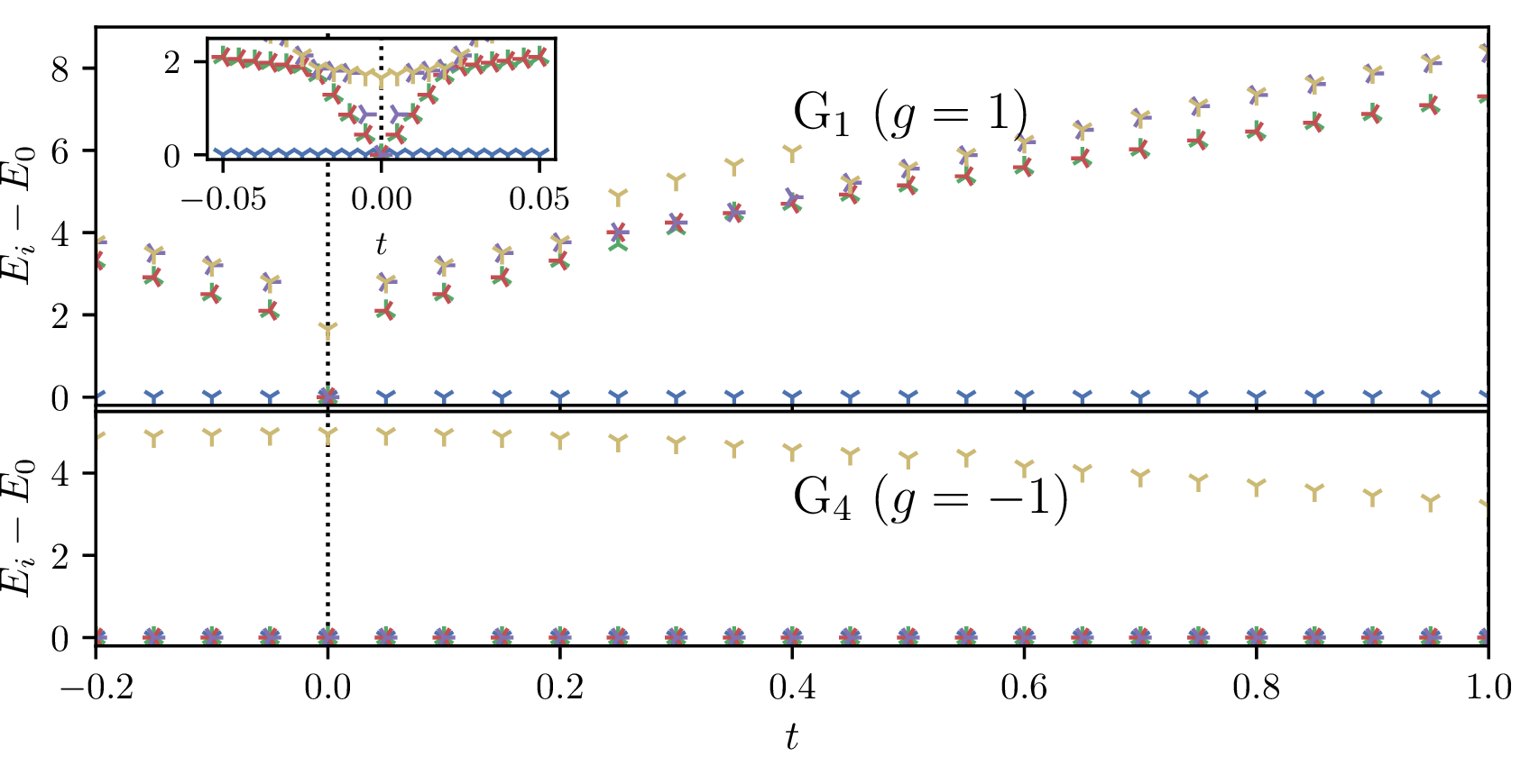
The strong-coupling (\(g\rightarrow \pm \infty\)) limits of the TLMH may be easily approached by fixing \(g\) to a finite value and scaling \(t\rightarrow 0\). To ascertain the fate of the G\(_1\) phase in this limit, we begin with \(g=+1\). As shown in Fig. 3, the gap protecting this phase closes at precisely \(t=0\) (equivalently, at the limit \(g\rightarrow \infty\)). The inset subplot shows a clear first-order transition at this point. Contrasting this, the G\(_4\) phase (found by setting \(g=-3\)) is stable in the \(t\rightarrow 0\) limit, with no gap closing or change in the four-fold ground state degeneracy anywhere in this limit. Noting that a gauge transformation allows us to map the interaction Hamiltonian \(H_I\) to \(-H_I\), we should find the same phase in both limits [2]. This is consistent with the four-fold ground-state degeneracy found at \(t=0\) in the \(g=1\) and \(g=-3\) cases, with the degeneracy occurring only at this precise point in the \(g=1\) case (due to a level crossing involving four states). Thus, our phase diagram in the main text indicates the G\(_4\) phase occurs at both \(g=\pm \infty\) limits. By examining the vicinity of this point in close detail, it is clear that the three states joining the ground state in the \(g=1\) G\(_1\) case correspond to high energy (rather than low-lying) excited states at \(t=1\).

4 G\(_3\) and GL\(_4\) phases↩︎

Fig. 4 plots magnetic and fermionic correlations in the G\(_3\) and GL\(_4\) phases computed on a cylinder with \(L_x=96\). This plot makes clear a six-site repeating structure in the G\(_3\) phase. Correlations in the GL\(_4\) phase are less easily understood. Notably, this phase exhibits long-range connected correlations in \(\sigma^z\), which are absent in the gapped SPT phases.

Like the G\(_4\) phase discussed in the main text, the GL\(_4\) phase exhibits a four-fold ground-state degeneracy on tori that doubles to eightfold on the torus. However, unlike the G\(_4\) phase, in which the gap \(\Delta\) separating the ground state manifold from the remainder of the spectrum remains finite as \(L_x\rightarrow \infty\), the GL\(_4\) phase exhibits a gapless spectrum. Finite-size scaling on \(x\)-OBC systems, shown in Fig. 5, indicates \(\Delta\propto 1/L_x^2\) as \(L_x\rightarrow \infty\).

5 Phase transitions with open boundary conditions↩︎

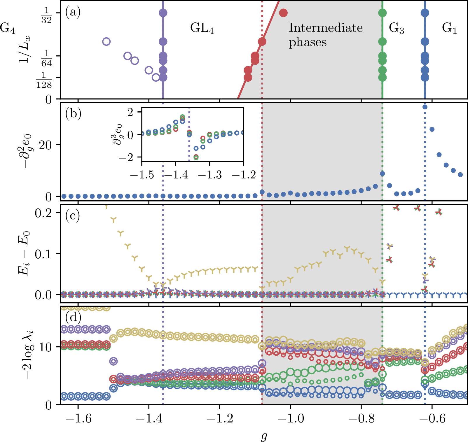
Fig. 3 in the main text depicts the phase transitions seen in the TLMH on a torus via energy susceptibility \(-\frac{\partial^2 e_0}{\partial g^2}\) and the entanglement spectrum \(\lambda_i\). Fig. 6 similarly depicts the phase transitions for cylindrical (\(x\)-OBC) systems. Since DMRG is better-suited for these systems, we were also able to obtain well-converged excited states on these systems, allowing us to study the gaps depicted in subfigure (c).

Other than the differences in degeneracy discussed in the main text, the G\(_1\) and G\(_3\) phases appear similarly. However, differences arise in the GL\(_4\) phase and surrounding transitions. Firstly, due to the degeneracy between the parity sectors on the cylinder in both G\(_4\) and GL\(_4\) phases, we cannot detect the transition by a switch in ground-state parity as on the torus.

On the cylinder, the phase transition manifests as a discontinuity in the third derivative of the ground-state energy, as shown in the inset of subfigure (b). At this same value of \(g\) (\(g\approx -1.36\) in all system sizes shown in Fig. 6), the gap above the degenerate ground-state manifold closes and the spectrum changes from gapless to gapped.

An interesting finite-size anomaly occurs at this transition: the ground-state entanglement spectrum plotted in subplot (d) doesn’t indicate a phase transition until a much larger value of \(g\approx-1.5\) for the \(L_x=48\) system shown. This would seem to be due to the fact that the bulk gap closing at \(g\approx-1.36\) doesn’t, in a finite system, involve the true ground state due to finite-size splitting, but instead only has immediate effect on higher-energy states within the ground-state manifold. As indicated by open circles in subfigure (a), the coupling at which these discontinuities occur approaches \(-1.36\) as \(L_x\) increases.

6 Odd-\(L_x\) torus: phase transitions and gapless mode.↩︎

By focusing only the odd-\(L_x\), \(x\)-APBC case in DMRG simulations, previous work on the 4-leg TLMH found a gapless phase [2] in place of the gapped G\(_4\) phase discussed in the main body of this text. Our DMRG simulations on odd-\(L_x\) systems suggest that the gapless mode occurs on tori regardless of \(x\) boundary condition (PBC or APBC), while odd-\(L_x\) cylinders instead host the gapped phases seen elsewhere. Here, we share some of our results on odd-\(L_x\), APBC systems. While our phase diagram still shows additional phases as compared to the prior work, we do find the same gapless phase.

Fig. 7 plots energy susceptibility and entanglement entropy computed from an \(L_x=19\) \(x\)-APBC torus. As indicated in the figure, we observe the G\(_1\) and G\(_3\) phases as before. This is followed by a difficult-to-analyze region with a number of apparent phase transitions. Following this, we observe a single phase for the range of couplings \(g\) that are split between GL\(_4\) and G\(_{4}\) phases in other geometries. While prior work identified a unique ground state in this region for odd \(L_x\) [2], we find a twofold degenerate ground state.

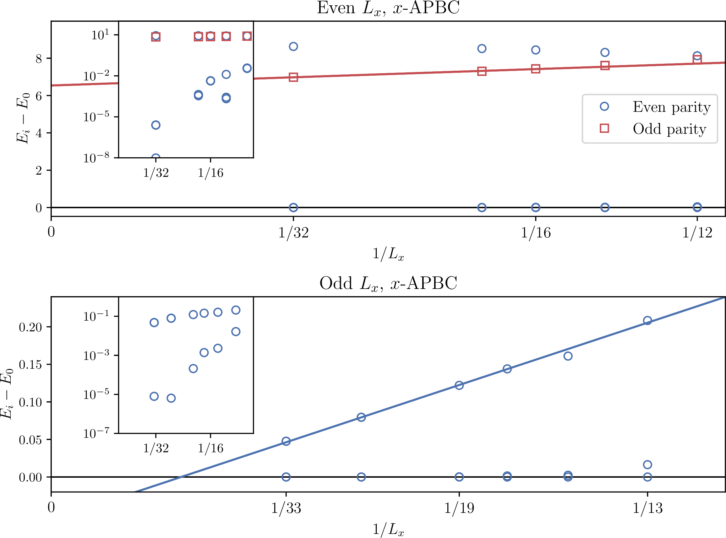
Analysis of gaps in this phase show \(1/L_x\) scaling consistent with a relativistic gapless mode. Fig. 8 compares these gaps (computed at \(g=-3\)) with those in even-length tori (which are in the G\(_4\) phase for this value of \(g\)). Both our results and those presented in earlier work [2] have a strange feature: the \(1/L_x\) gap scaling extrapolates to a negative, finite gap as \(L_x\rightarrow \infty\) rather than zero gap as should be the case. While this would seem most likely to be a finite-size effect of some sort, difficulties in DMRG simulations (resulting from both the required periodic boundaries, the highly-entanglement nature of the eigenstates, and the twofold degeneracy of the ground state) prevent us from obtaining the excited states required to compute these gaps for \(L_x>33\).

Further support of the gapless nature of this phase can be found by examining its central charge \(c\). We follow the approach taken in earlier work [2], which assumes our system is well-described by a 1+1-dimensional CFT on our \(N\)-site lattice. Given such a situation, the entanglement entropy for a bipartition at the \(x\)th site is predicted to fit the formula \[S(x)=\frac{c}{3}\log\left[\frac{N}{\pi}\sin\left(\frac{x\pi}{N}\right)\right] + S_0 \label{eqn:s95charge}\tag{11}\] where \(S_0\) is a non-universal constant [3]. To account for an even-odd effect, we replace \(S(x)\) with the entanglement entropy averaged over two adjacent sites, \(S(x')=\frac{1}{2}\left(S(x)+S(x')\right)\) with \(x'=x+\frac{1}{2}\) [2]. In practice, we obtain \(c\) by obtaining a least squares fit of \(S(x')\) as a function of \(\ell(x')=\frac{1}{3}\log\left[\frac{N}{\pi}\sin\left(\frac{x\pi}{N}\right)\right]\), with the data restricted to the largest few values of \(\ell\) to avoid short-range physics.

Entanglement entropies and best-fit lines indicating central charges of \(c\approx 1\) at \(g=-3\) (in the gapless phase) are shown in systems ranging from \(L_x=33\) to \(L_x=65\). In all cases, bond dimensions were chosen to maintain a DMRG truncation error of at most \(10^{-6}\), with the \(L_x=65\) case requiring a bond dimension of \(m=2500\). In all cases, values of \(c\approx 1\) were obtained.

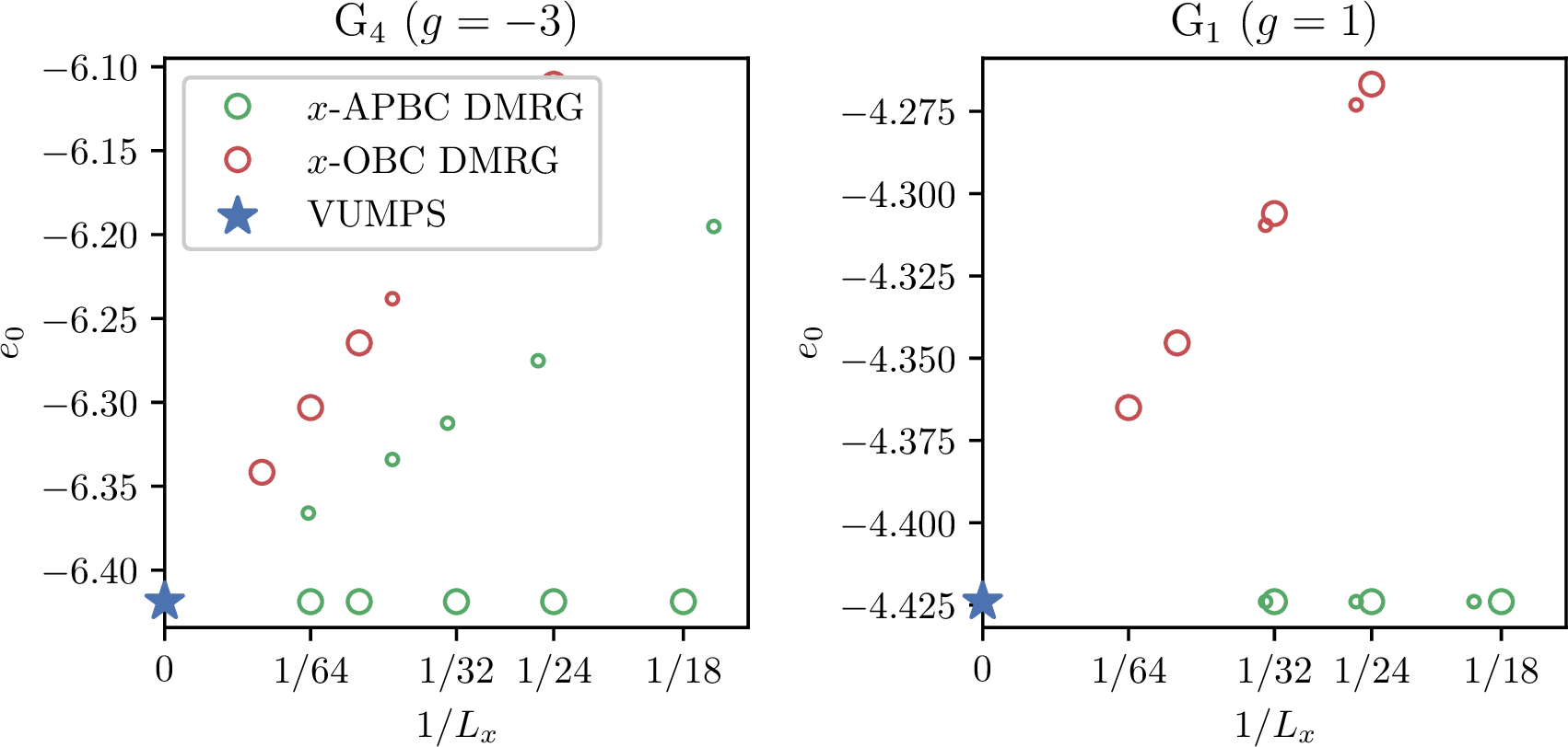
As discussed in the main text, we hypothesize the gapless phase is an anomaly most likely caused by a frustration-induced, deconfined domain wall. Comparison of energy densities \(e_0 =\frac{1}{2 L_x}E_0\) in Fig. 10 from different boundary conditions and system sizes indicates this gapless mode corresponds to a higher-energy ground state than similar-sized even-\(L_x\) periodic systems, with energy difference shrinking as \(1/L_x\) in the thermodynamic limit and in all cases extrapolating to the value of energy density obtained from VUMPS for an infinite-MPS ground state.

This scaling in energy density is consistent with the formation of a domain wall (or other defect) at a cost of \(\mathcal{O}(1)\) in energy, thus leading to a \(1/L_x\) penalty in the energy density. A similar energy penalty occurs for \(x\)-OBC systems with \(L_x\) even or odd, which can be ascribed to the absence of \(\mathcal{O}(1)\) terms in the Hamiltonian connecting the ends of the cylinder. The lack of these energy-reducing terms causes a \(1/L_x\) increase in energy density.

References↩︎

---

1. In our notation, \(L_y\) corresponds to the number of Dirac modes (unit cells) along the \(y\) direction, not the number of rows of the underlying triangular lattice.↩︎

2. Note that while finite-size scaling results for DMRG are not presented in this figure, they are shown later in Fig. 10 at \(g=1\) and \(g=-3\), with both cases indicate a minimal change in energy density (\(\mathcal{O}(10^{-3}\)) as opposed to the \(\mathcal{O}(1)\) discrepancy observed between finite-size exact (DMRG) energy density and either finite-size or infinite-system mean-field energy densities for \(g<g_1\).↩︎