1 Introduction↩︎

The solar corona is in a state of constant change, as the interplay between the magnetic fields and mechanical forces drive dynamics at every length scale and temporal cadence imaginable. Despite major progress across many domains, there are still significant open questions. These include the so-called “open flux problem” [3]–[5], wherein there is a discrepancy between the in-situ measured heliospheric open flux and that which is estimated from coronal observations. Another prominent set of questions concerns where, how much, and what types of plasma populate the solar wind from different source regions in the low corona [6]–[12]. These questions are challenging to close because, while we have observations of the low corona and in-situ observations, there are few if any direct observations connecting them, and many different scales, physical transitions, and processes are involved in the vast distances between them [13]–[18].

Theories like the S-web [8], [19] attempt to connect these regions and explain how plasma on field lines all over the Sun will distribute itself, accelerate, and possibly escape as it moves through the corona. The theory maps out the regions of high or low magnetic convergence, highlighting regions such as coronal holes, streamers, and null-point topologies. Visualizing the three-dimensional signatures of these regions as they evolve with time and height is important to understanding both low-coronal dynamics and solar wind development and evolution [20]. However, connecting frameworks such as the S-web with the actual behavior of the plasma populating the magnetic framework is often not straightforward, even within the ranges for which we have observations [21]–[23].

One of the primary mechanisms highlighted by S-web theory is topological change, which is the main topic of this paper. There are several types of topological change, briefly summarized here. Closed-closed reconnection is the exchange of footpoint identities between two closed magnetic field lines, which results in two more closed magnetic field lines; in other words, the identity of the loops changes, while their classification (two closed field lines) does not. In open-closed (or interchange) reconnection, one open field line and one closed field line exchange footpoints, resulting in the opening of the closed field line and the closing of the open field line. Here, as with closed-closed reconnection, the identity of the loops changes (one opens, one closes), but their classification does not (one open field line, one closed field line). Open-open reconnection, on the other hand, involves “pinch-off” reconnection between two open field lines, resulting in one disconnected field line and one closed field line. Here, both the identity and the classification changes. Finally, a closed loop can expand outward to large distances, dragged out by the solar wind, or as part of a CME. From the coronal point of view, this field line can be considered open when its apex is beyond the Alfvén surface. Within the context of the MHD model, it will be identified as two open field lines when the apex crosses the outer boundary.

The magnetic fields in the corona respond to the evolution of the photospheric magnetic field. Models strive to quantify this response. To that end, the advent of surface flux transport models [24]–[27] has hastened the adoption of time-dependent MHD modeling, which in turn has produced more realistic results than steady-state models [28], [29]. These advances also provide the opportunity to revisit common methods of analysis and to develop novel tools that can extract the most useful information possible from new and improved simulations. In other words, making the most of time-dependent models requires time-dependent analysis tools.

In this paper, we present a new application of slip-back mapping (SBM), first introduced in [2]. SBM allows users to investigate magnetic flux evolution and identify some of the mechanisms by which topological change is occurring throughout the simulation, with better accuracy than previous tools. This method, which depends upon thorough knowledge of the inner boundary’s flows, is necessary due to the inner boundary’s evolution in a time-dependent model. Position is no longer sufficient information to track flux evolution; each field line moves with flows, so the net advection of the parcel must be taken into account in order to accurately trace a given field line. SBM calculates these traces with a tunable time step, allowing for large-scale analysis of topological change across the entire corona. We apply this method to the time-dependent Magnetohydrodynamic Algorithm outside A Sphere [30] simulation first presented in [31]. Section 2 discusses the background and details of the code and the time-dependent mode. Section 3 covers the background and overview of the SBM method (more specific details of the algorithm are provided in the Appendix), and includes some notes on the interpretation of the raw method output. Section 4 presents the results of the investigation, focusing on open flux evolution and the aggregated topological changes in the model, while Section 5 discusses the implications of the findings for our understanding of the dynamic corona, both in theory and data analysis.

2 MAS↩︎

MAS solves the thermodynamic, resistive MHD equations on a nonuniform spherical mesh; these equations describe coronal heating, thermal conduction parallel to the magnetic field, and radiative losses. It uses a semi-implicit time-stepping algorithm, and covers the global corona and solar wind [30], [32], [33]. The thermodynamic MHD approach allows the plasma density and temperature to be computed with sufficient accuracy to forward-model EUV and soft X-ray emission and other remote sensing observables [32], [34]–[36]. The coronal domain extends to 30 \(R_\odot\), where outflows are typically super-Alfvénic (simplifying the outer boundary conditions). A wave-turbulence-driven (WTD) approach is applied for coronal heating and solar wind acceleration to model the large-scale solar wind properties [35], [37]. MAS has produced state-of-the-art solutions of the corona for case studies of its structure and connectivity [29], [35], [38], [39], coronal mass ejections [40]–[43], and the inner heliosphere in general [33], [44].

Recently, MAS has incorporated a method for evolving \(B_r\) at the inner boundary, \(B_{r0}(\theta,\phi,t)\), such that it matches the values supplied by the flux transport model. The evolution is specified via the tangential electric field at the boundary, \[E_t = \nabla_t \times \Psi \hat{r} + \nabla_t \Phi,\]by solving for two scalar potentials, \(\Psi\) and \(\Phi\) [35], [45], the first of which controls the \(B_r\) evolution. When employing flux-transport models and maps, the large-scale flows (differential rotation and meridional flows) influence the long-term field evolution; these are included in the second, non-inductive potential. The strength of the method is that all known boundary flows can be incorporated into \(E_{t0}\), while ensuring that \(B_{r0}(\theta,\phi,t)\) always matches the specified values [31]. Freedom in the second potential can also be further adapted for the introduction of energization. However in this case, this potential is not used to inject additional shear, helicity, and magnetic energy at large-scale neutral lines [29], and as such, this model represents a minimally energized corona evolving at solar minimum.

For this study, we use the original time-dependent simulation in MAS [28], [31], in which the evolving maps of the photospheric field were provided by the Lockheed Evolving Surface-Flux Assimilation Model [24]. In this case, a “synthetic” sun was simulated, with the evolving surface fields scaled and distributed such that they approximate the conditions near solar minimum. This model includes small- and large-scale flux emergence, flux decay, differential rotation, and meridional flows. Using fully synthetic data (created using observationally-derived statistical distributions) ameliorates many of the challenges in magnetic data assimilation methods, such as far-side flux emergence and global flux balancing. The sequence of \(B_r\) maps was utilized with a cadence of one hour of solar time per map; there were 721 maps in total, spanning \(\sim\)​30 days of physical evolution.

3 Slip-back Mapping↩︎

3.1 Anatomy of a Mapping↩︎

The algorithm behind the slip-back mapping (SBM) method was originally outlined in [1] and expanded in [2]. Specific details on the implementation of SBM for this time-dependent run can be found in the appendix of this paper, but we describe the method in general terms here.

To begin, consider two times in a time-dependent simulation, which we designate \(t_0\) and \(t_1\). Two slip surface locations are designated from which the mappings begin or end: in this study, the inner and outer slip surfaces are located at \(r=1.01\) and \(r=19 \,R_\odot\), respectively.

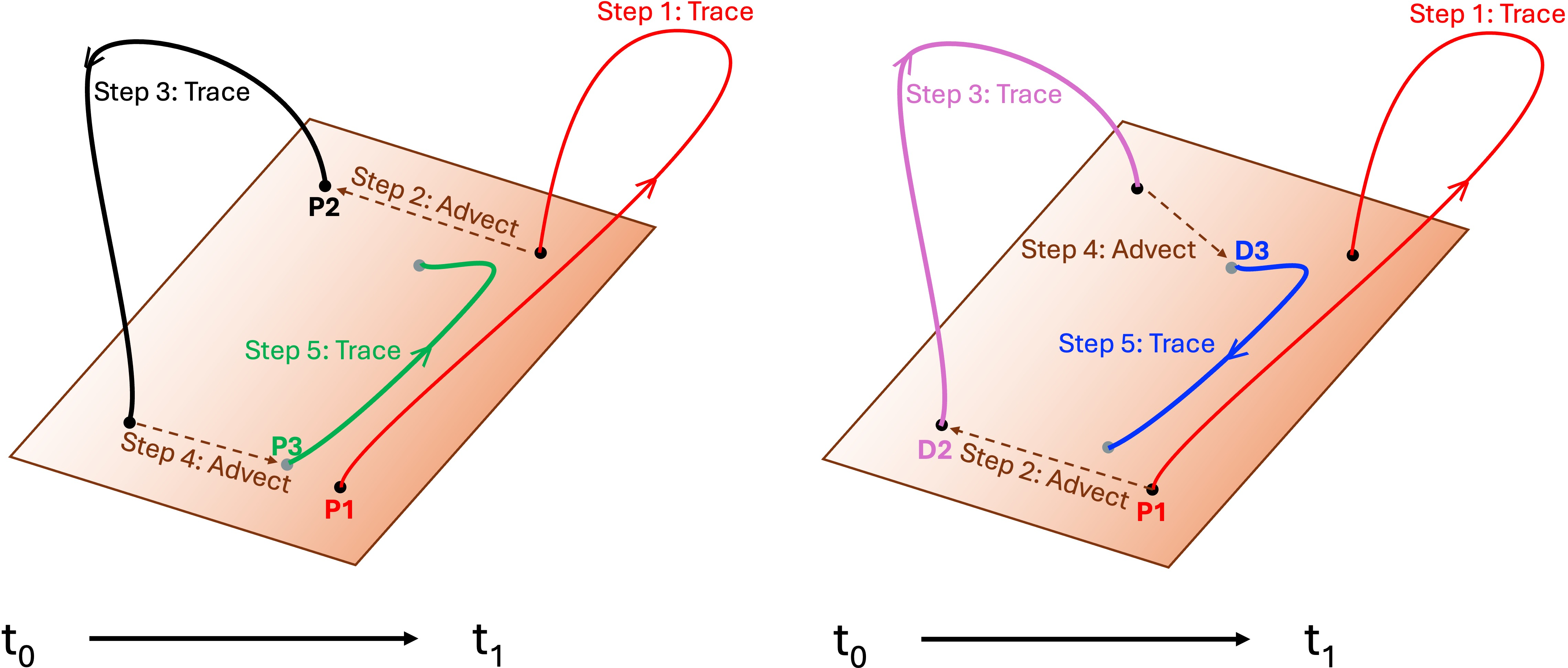
To begin a mapping, the intersection of a magnetic field line with the slip surface (P1) is selected at \(t_1\), and the field line is traced to its opposite end. The other end may either be located on the same slip surface – for a closed or disconnected loop (depending upon whether the mapping begins from the inner or outer slip surface, respectively) – or on the opposite slip surface for an open field line. This is step 1 as shown in Figure 1.

After this first step, there is a divergence in the algorithm for the primary (Fig. 1a) and dual (Fig. 1b) mappings. For the primary mapping, the opposite footpoint is advected backward from \(t_1\) to \(t_0\) using the net flow in the plane of the slip surface, termed \(v_{tfl}\). For the dual mapping, it is P1 which is advected backward in time. In either case, this is marked as step 2 in the figure. Again, the field line from P2 (or D2) is traced in step 3, and the footpoint is advected forward in time in step 4 to find P3 (or D3) at \(t_1\). This point is then used to trace the final field line, completing the process in step 5.

Each theta-phi location on the simulation grid is then subjected to this process to build up the full map, and the connection values of each point (P1, P2, P3, D2, D3) are recorded. We use a value of 0 for a closed field line, 1 for an open field line, and 2 for a disconnected field line. These values are given in the order D2 P2 P1 P3 D3, resulting in a 5-digit value in base-3. P2 and D2 are from \(t_0\), while the other three are from \(t_1\), hence the order. This 5-digit value is converted to base 10 and saved as the SBM value for that pixel, resulting in a final 2D theta-phi map for a given time range and cadence. When discussing specific codes, we refer to them in the same order but by their mappings, such as OC-CO/O.

As a simple example, we show SBM code OC-CO/O in Figure 2a. The traced field lines are colored using the same convention as the footpoints are labeled in Figure 1ab; namely, P1 in red, P2 in black, P3 in green, D2 in purple, and D3 in blue. This scenario, which carries the value 109 in the SBM map, represents an interchange reconnection case. Here, the field lines at \(t_0\) are open and closed respectively (the OC at the beginning of the code), while both the primary and dual mappings return field lines at \(t_1\) which are closed and open (both return CO, indicating the connectivity has swapped between the two field lines). Order matters in the code; OC-CO/O, for example, is not the same as OC-OO/C. The first indicates that the primary mapping indicates interchange reconnection and the dual mapping has identified an adjacent field line, while the second indicates the reverse (note: neither is the code mapped in Fig. 2). A simple example of interchange reconnection that is directly analogous to (a) is shown in Fig. 2bc. Reconnection in particular can be challenging to track in this way, as discussed in Section 4.

3.2 Notes on the Method↩︎

There are a few important aspects of the SBM process that the reader should note. Although the MAS algorithm advances the vector potential and conserves magnetic flux to machine precision, the SBM calculations use the magnetic field output, which, when interpolated to obtain values at different locations, may not exactly preserve this property. Furthermore, the existence of a discrete outer boundary (in this case, the outer slip-surface) leads to some flux leaving the domain and being lost from the system. Similarly, a closed loop whose apex is advected outward will artificially be categorized as two opening field lines. These causes are well-known limitations shared by all MHD simulations. Lastly, flux can be lost or misidentified through propagated advection errors. These can build up when the output cadence of the 3D velocity data is larger than the time step of the MHD algorithm. Optimally, the SBM would be calculated by the MHD code during each time step. However, conducting this step as part of the run itself is time-intensive, so in practice we calculate it ex post facto using the simulation outputs.

SBM may be performed beginning from either the inner or outer slip surface, and in fact the mappings will not have a 1:1 correspondence. This is because some cases involving disconnected flux can only be detected from the outer slip surface. For this study, all calculations were made from the inner slip surface, as this is the more relevant case for coronal investigations.

In reference to the process in general, the arrows shown in Fig. 1 designate the direction of the trace, not the direction of the magnetic field. In fact, the direction of the trace sometimes opposes that of the field, because the first trace (from P1 in step 1) is always outward from the slip surface. This may be with the magnetic field (if P1 is located in positive field) or against it (if P1 is located in negative field). Since the dual mapping advects P1 back in time, it must trace in the same direction, as D2 must be the same polarity as P1. By contrast, the primary mapping advects the slip-surface’s point of intersection at the opposite end of the field line back in time, so that tracing must go in the opposite direction.

Finally, SBM can be calculated for any desired cadence (as long as the simulation produced data at the desired rate), and indeed the results here reflect data from two separate calculations, one at a 6-hour cadence and one at a 24-hour calculation. The latter is used only for Fig. 5 and its associated animation. The process described above assumed that \(t_0\) and \(t_1\) were separated by a single time step for simplicity, but the process only changes in that there are more advections backward or forward for each intervening time step, in order to maintain an appropriate trace.

3.3 Scale-Based Analysis Recommendations↩︎

Although the method relies on tracing field lines from every point along the grid and tracking those field lines backward and forward in time in accordance with the slip-surface flows, interpreting individual cases involves a thorough understanding of the process used to create the maps. SBM can certainly serve as a method by which to zero in on small-scale regions undergoing rapid topological change, and to easily illustrate the relevant reconnection mechanisms occurring. However, caution must be exercised when analyzing individual cases. The flux involved in the topological change can be of the same order of magnitude as the uncertainty in the flux measurement itself, depending upon the strength of the field at that location and the grid size of the simulation. This, coupled with the uncertainty in the mapping that can be introduced by loops shorter than the slip-surface height (discussed in Sec. 3.2), can result in confusing results for the unwary user. We therefore strongly recommend binning the codes into a few categories as we have done here, and it is of the utmost importance to evaluate and understand each code before determining to which category it belongs.

4 Results↩︎

Raw SBM maps are arrays of several hundred unique code values, spread out across a theta-phi map in a pattern reminiscent of a cobweb. This is difficult to visualize clearly or to interpret. In order to turn these disparate individual events into an intuitive dataset, we binned the values into six main categories. These categories are defined by the physical mechanism they represent, and whether it is the primary or dual mapping that identifies the mechanism. The mechanisms are flux opening (FO), flux closing (FC), and disconnection (DC). For primary mappings, we compared the state of P1 (open or closed) to the state of P2 (which could be open, closed, or disconnected). If P1 was open and P2 was closed, the code belonged to FO; the opposite situation belonged to FC. An analogous categorization held for the dual mapping, with a comparison between P1 and D2. Disconnected codes include a disconnection value at \(t_1\) that is not already in the FO or FC category, to avoid double-counting between the mechanism bins (double-counting also occurs between the dual and primary mappings, which we handle by dividing the sums of these values in half, as shown in the equations below). If either the primary or dual mapping had no change between \(t_0\) and \(t_1\) (i.e., both P1 and P2/D2 were open, or both were closed), the code was not included in the following statistics for that bin.

For example, the code OC-CO/O shown in Fig. 2a would be discounted from the primary categorization because both P1 (at \(t_1\)) and P2 (at \(t_0\)) are closed; however, it would be included in the dual categorization as FC, since P1 is closed but D2 (at \(t_0\)) was open. This method, of course, includes interchange reconnection as well as more straightforward flux opening or closing, such as helmet streamer growth (where closed magnetic field lines’ apexes pass outside the outer boundary of the simulation, becoming de facto open field) or pinch-off. We discuss how we recover the interchange reconnection fluxes from the FO and FC bins below.

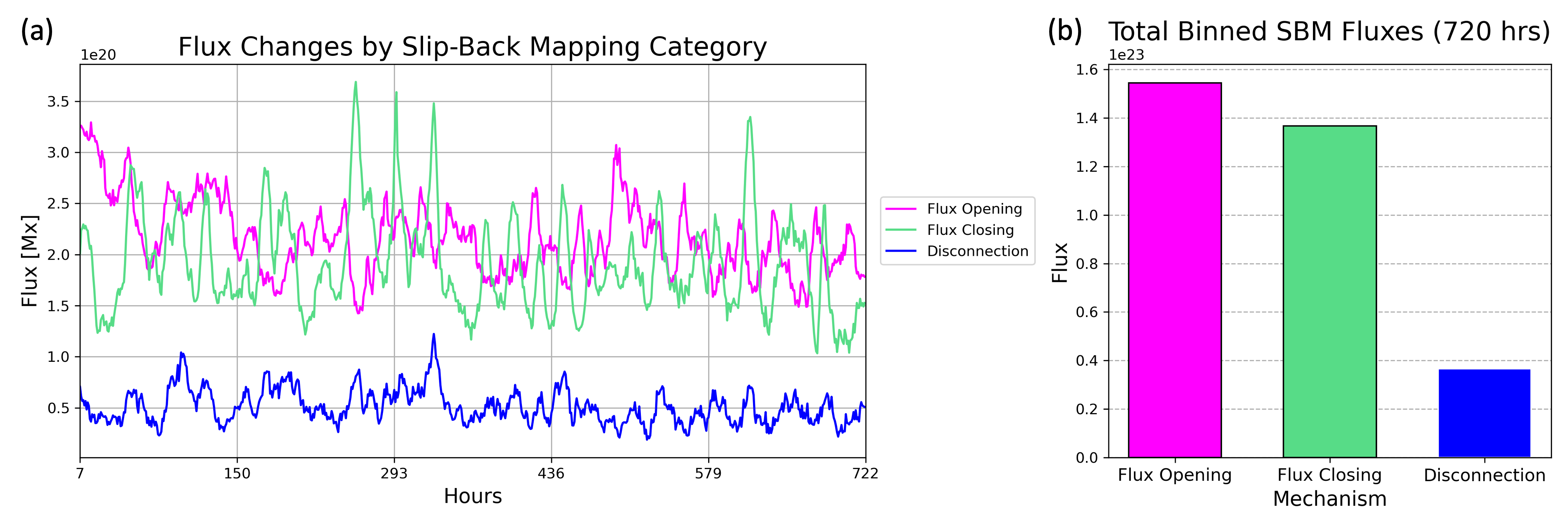
Figure 3a shows the evolution of these categories of SBM fluxes over time, using a 6-hr cadence for the mapping on the full 721-hour simulation. The FO and FC categories show much higher overall fluxes and more variability than the DC category, as expected from a SBM applied to the inner slip surface. Overall, the FO slightly exceeds the FC category, as can be seen more clearly in Figure 3b.

The top plot of Figure 4 shows the evolution of the change in open flux (\(\Delta OF\)) over the course of the simulation. The black line shows the standard \(\Delta OF\) calculation for the simulation – that is, the differencing of 6-hour windows of the open field calculated from the model outputs. The SBM-based \(\Delta OF\) is plotted in red, and the unsigned \(\Delta OF\) associated with interchange reconnection is plotted in blue. Explanations of both derivations follow.

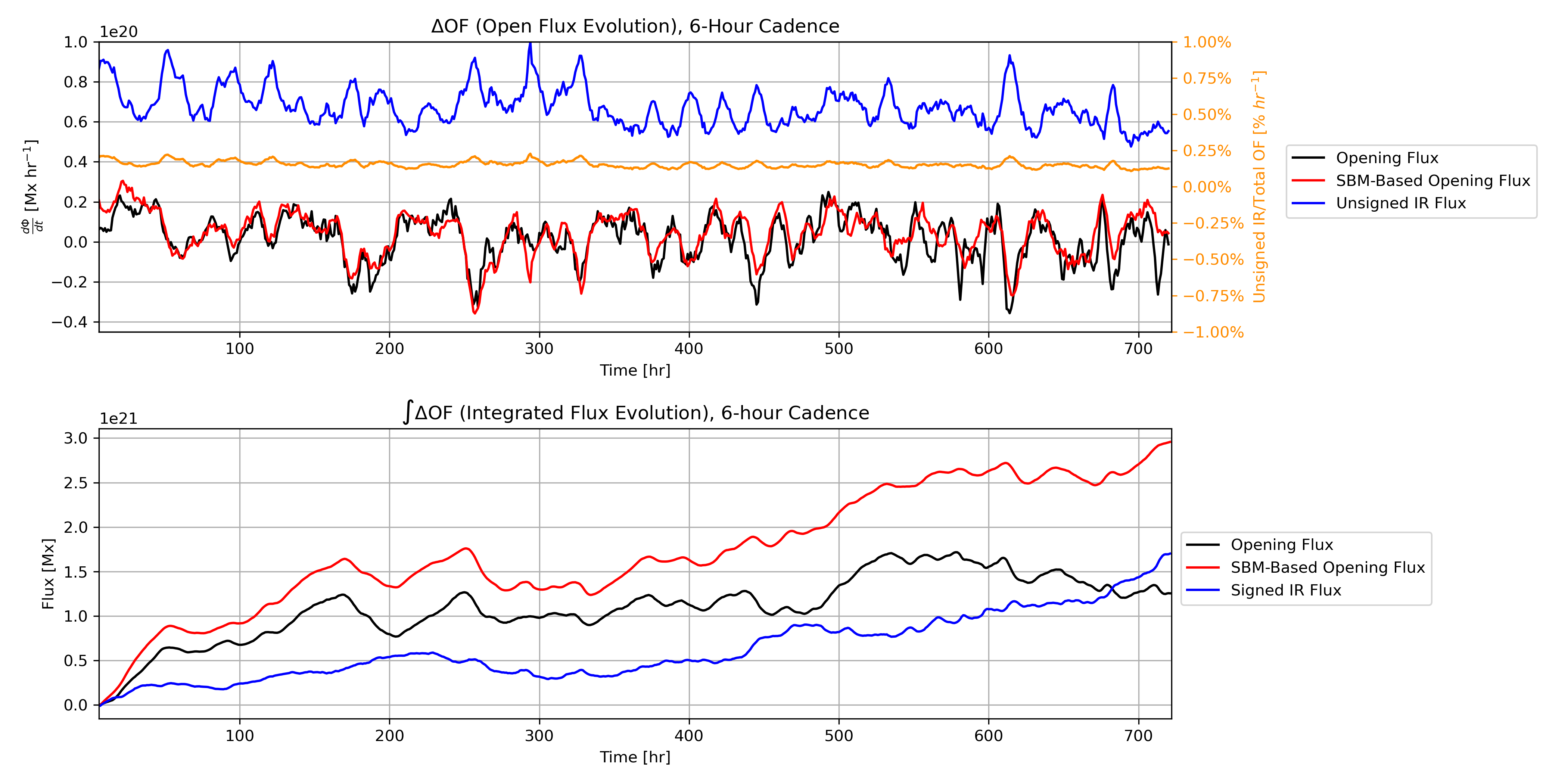
While the SBM calculation itself uses 6 hourly time steps to compute each map, the maps advance by a single time step for each calculation (i.e., one slip-back map covers hours 1-6, the next covers hours 2-7, etc.). Thus, the time derivative itself is still per hour. The \(\Delta OF\) using the slip-back maps is computed using the following definition: \[\Delta OF_{SBM} = \frac{1}{2}[(FO_{dual}-FC_{dual})+(FO_{primary}-FC_{primary})],\]where \(\Delta OF_{SBM}\) is the change in the total open flux, \(FO_{dual}\) is the flux measured as opening in the dual mapping, \(FC_{dual}\) is the flux measured as closing in the dual mapping, \(FO_{primary}\) is the flux measured as opening in the primary mapping, \(FC_{primary}\) is the flux measured as closing in the primary mapping. The factor of one-half is included to remove the double-counting inherent in the categorization method.

One of the main goals of the SBM method is to trace regions where interchange reconnection is likely to occur, but this is challenging for several reasons. As discussed in Section 3, the categorization system used here does not include interchange reconnection separately, largely due to the challenge posed by identifying it. The very nature of interchange reconnection complicates flux calculations, as there is no net change in the open flux. Additionally, resistive MHD is unable to realistically capture the microphysics involved in magnetic reconnection, but general dynamics can be well reproduced. The introduction of the slip surface also excludes detection of any closed field that lies below the slip surface’s location, although it is of central importance. Flux emergence would cause failures in the calculation if the inner and outer boundaries were the surfaces from which the SBM was generated; the slip surfaces are located at heights corresponding to a characteristic radial advection distance (this advection speed is much lower for the inner boundary, which is why the inner slip surface is located only 0.01 \(R_\odot\) above the inner boundary, which the outer slip surface is located 1 \(R_\odot\) below the outer boundary). Therefore, there are many cases – particularly involving small parasitic bipoles in coronal holes – where very short field lines are excluded from the calculation entirely. However, interchange reconnection can be recovered using the values plotted in Figure 4. Using \[IR{_{US}} = \frac{1}{2}[FO_{dual}+FC_{dual}+FO_{primary}+FC_{primary}]-OF_{total},\]where \(OF\) is the open flux from the simulation, we recover the total unsigned flux involved in interchange reconnection. The signed interchange reconnection flux can be found similarly: \[IR_{S} = \frac{1}{2}[(FO_{dual}-FC_{dual})+(FO_{primary}-FC_{primary})]-OF_{total},\] which is equivalent to \(\Delta OF_{SBM}-OF_{total}\). The bottom plot of Fig 4 shows the cumulative open fluxes, and the cumulative signed interchange reconnection flux is plotted in blue.

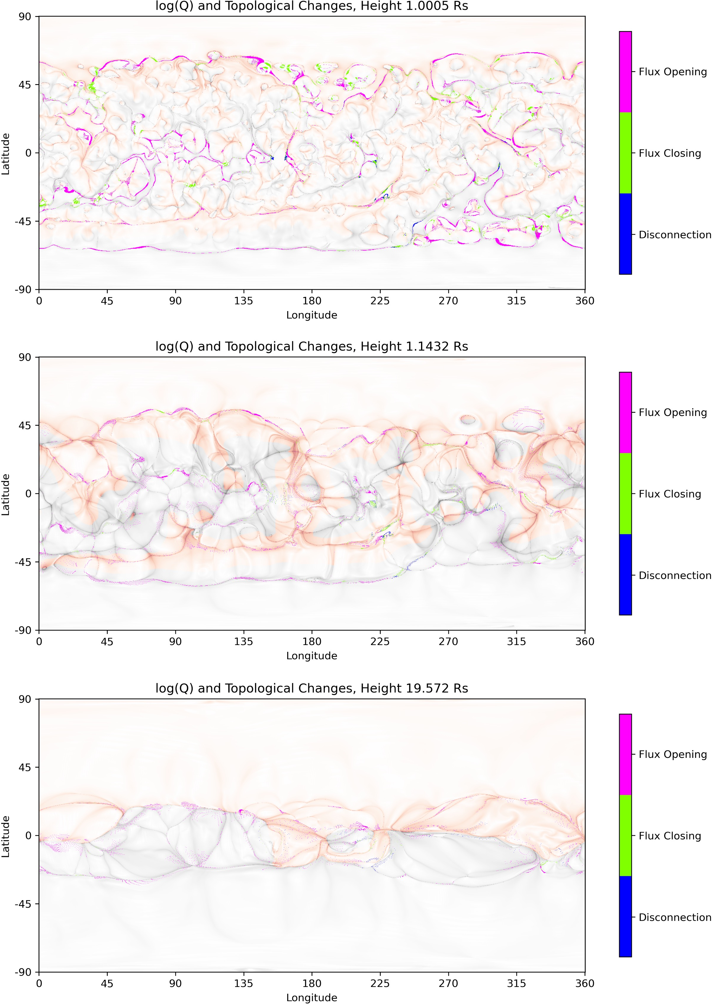
Figure 5 shows three panels at the same time step, but at different heights within the simulation. The red/gray map shows the squashing factor (or Q), scaled logarithmically and signed for magnetic polarity. Over this is plotted the intersection with the plotted height of every field line involved in a SBM code, colored by category. The three heights shown here are extracted from the full animation (available in the online version of the paper) which shows the progression in height from 1 to 19 \(R_\odot\) at a single time. This visualization provides perspective on how these field lines align with the major magnetic structures in the corona. As can be seen in the figure and the animation, the SBM field lines lie almost entirely along high-Q lines. While the over-plotted points appear widely distributed in the low corona, as the height increases it becomes obvious that the FO codes predominate along the heliospheric current sheet (seen as the main boundary between the red and gray sectors in the map), while the FC and DC codes tend to show up near quasi-separatrix layers (QSLs), or pseudostreamer arcs (visible as high-Q lines that lie entirely within one polarity). In theory, over time all three codes should occur along both types of arc. However, at a given time, it is more likely to observe this distribution. FO is often associated with the longest helmet streamer field lines growing beyond the slip surface, where their coding changes from closed to open. This is more common and less impulsive of an occurrence than helmet streamer pinch-off, where FC and DC codes would be expected to predominate locally. The high rates of interchange reconnection associated with the null-point topologies that plot as QSLs, on the other hand, are very likely to show a mix of all three bins at any given time, as seen here.

5 Discussion↩︎

5.1 Time-Dependent Analysis↩︎

We have described the algorithm behind the SBM method and applied it to a fully time-dependent thermodynamic MHD simulation covering a month of solar evolution. The time dependence of the SBM method is central to its nature, and a necessary advance in MHD analysis tools. As our modeling capabilities continue to improve, so must our tools evolve to take the best advantage of the enhanced results. SBM is an inherently time-dependent metric, developed for time-dependent simulations. As we show in Fig. 4, SBM tracks the open flux evolution in a time-dependent model without necessitating the assumption of a potential field, and it can also be used to find the OF at any one time. We have focused here on the full codes, since the investigation’s goal was to trace the major trends in topological change, but more traditional quantities can also be recovered from a single mapping.

The method really excels in the aggregate, where binning multiple SBM codes together allows for the creation of maps and animations that show how and where flux is being processed throughout the corona and into the solar wind. The binning choices made in this paper are far from the only way to categorize these codes. Other categorizations would allow researchers to zero in on specific types of topological changes – for instance, to focus on reconnection dynamics at the heliospheric current sheet like streamer blow-out or pinch-off events. Alternatively, one could focus solely on the codes that associate with small-scale interchange reconnection, to investigate the evolution of very small null-point topologies. Yet another avenue of research would be to map from the upper slip surface to gain insights on the open and disconnected field in the solar wind as it propagates outward. Some of these will be the focus of future work, but we include a wide range of ideas as inspiration to others in the adoption of this method for other time-dependent models.

5.2 Solar Wind Implications↩︎

While developing this methodology, we experimented with a broad range of cadences for the mappings, ranging from 3 minutes to 24 hours. We consistently found that – while specific codes may shift with cadence – categorized trends did not. For example, a high-Q arc that was predominantly populated with FO codes tended to remain an arc of predominantly FO codes, although more FO codes generally accumulated in the area as the cadence period increased. We chose the 24-hr cadence for Fig. 5 since it allowed reasonable visibility of the patterns created by the mapping, while the rest of the plots illustrate slip-back calculations made with a 6-hr cadence. The 6-hr cadence was chosen as a time frame that agrees well with typical solar wind propagation speeds from the inner to the outer boundary of the calculation, allowing us to investigate the dynamics in the inner corona that contribute to the solar wind.

A coherent and compelling picture emerges from a comparison of the flux processed by the three main categories of topological change and the plot of the location of these changes with respect to a Q map. The total open flux for the simulation is around \(4\cdot10^{22}\) Mx on average. This means that for any given 24-hour interval, approximately 3.5% of the Sun’s open flux is processed through interchange reconnection, as defined by this investigation and using the values plotted in Fig. 4. It should be noted that this is specifically for a simulation scaled to approximate the conditions near solar minimum. During periods closer to solar maximum, greater magnetic flux emergence and more closely located regions of opposing polarities should lead to significantly higher proportions of open flux which has undergone interchange reconnection.

The field lines associated with SBM codes are widely distributed along high-Q lines low in the corona as shown in Fig. 5, with many appearing along QSLs. QSLs can be thought of as the projection of a null-point on the S-web, in much the same way as a null-point is itself the projection of a neutral line from the photosphere into the low corona. These arcs in the S-web indicate pseudo-streamers and smaller null-point topologies, and therefore are predicted to be strongly correlated to interchange reconnection. It is critical to note that Fig. 4 also shows that significantly more flux is processed by interchange reconnection than by field-opening or field-closing methods. We see this correlation reflected in Fig. 5, where the field lines associated with topological change definitively clustered along the lanes of S-web arcs. Although this study used a 6-hr cadence, a shorter cadence would highlight any “bursty” reconnection driven by higher-frequency changes in the flows, and could be used to compare to the temporal signatures of related observed solar wind phenomena, such as periodic density structures [47]–[49]. It should also be noted that this cadence does not separate individual reconnection events; it is reasonable to assume that many interchange reconnection events occur at these locations during this time, so the 1% result should be considered a lower bound.

5.3 Open Flux Implications↩︎

SBM provides a more nuanced view of open flux evolution, compared to a traditional open flux map derived from cell-by-cell connectivity traces at a single time step. This is because it retains the identity of the flux regions as they move through the advection tracing, rather than simply comparing the static locations based upon the grid of the simulation. By preserving the flux element’s identity, it simplifies certain questions, such as whether a region along a coronal hole boundary has merely moved or undergone a topological change. This is critical for improving the physical interpretation of simulation results, and can be used to better estimate reconnection rates, measure open flux evolution, and disentangle convolved mechanisms (e.g., rigid rotation of coronal holes).

While the results from the top panel in Fig. 4 show that the interchange reconnection-related flux is a few percent of the total open flux over any 24 hour interval, the bottom panel also implies that this is a relatively high proportion of the total open flux change over time. As mentioned previously, these results are derived from a simulation with relatively quiet solar conditions; a simulation such as the 2024 total solar eclipse prediction presented in [29] is anticipated to produce significantly higher proportions of such wind, and this will be investigated in future work.

5.4 Summary↩︎

Here, we presented results of the slip-back mapping method over a Carrington rotation of time, with individual codes highlighting localized magnetic field dynamics, as well as aggregated categorized maps to illustrate overall trends.

The single code cases allow isolation of interactions at the scale of single magnetic field lines and can help provide insights into changes at the smallest spatial and temporal scales of the simulation. While care should be taken when interpreting individual codes due to the constraints of the simulation’s resolution, they can also allow for more rigorous visualization of the behavior of small structures like jets.

The aggregated maps show how coronal plasma from closed field is released as solar wind concentrated primarily along S-web arcs. The ability to derive interchange reconnection rates using our method is new, and provides insight into what proportion of the solar wind should be anticipated to show closed-field abundances. Unsigned interchange reconnection flux dominates over open flux changes at every time in the simulation, providing additional evidence that this is a dominant dynamic in the corona. We found that approximately 3.5% of the open flux is processed through interchange reconnection over any 24 hour interval, which corresponds to a relatively high proportion of the total open flux changes over time in the heliosphere. These results are based on a solar minimum-like simulation with a minimal amount of free-energy injection, so these proportions are expected to increase for a more active scenario.

This paper illustrates the utility and importance of using time-dependent analysis methods for a time-dependent 3-dimensional magnetohydrostatic simulation. The slip-back mapping method scales well for dynamics at various ranges, and the aggregation plotting presented here reduces some of the dimensionality of the method for easier visual parsing. This is one of many tools which should be developed to enhance our understanding of time-dependent simulations.

6 Details of the Slip-back Mapping Algorithm↩︎

The algorithm described here is the natural evolution of that outlined in [1] and expanded in [2]. Two slip surfaces \(R_0\) and \(R_1\) are defined close to the lower and upper radial boundary respectively (\(R_\odot \lesssim R_0 \ll R_1< R_\mathrm{up}\)), and at two times: \(t_1\) (the present), and \(t_0<t_1\) (the past). The algorithm involves multiple steps, alternating tracing magnetic field lines and advecting points. Magnetic field lines are traced from different points at \(t_1\) or \(t_0\) by solving \[\frac{d \mathbf{x}}{d s} = \frac{\mathbf{B}(\mathbf{x})}{B(\mathbf{x})},\] with the predictor-corrector method. Here \(\mathbf{x}\) is the position in the computational domain, \(s\) the distance along the field line. The magnetic field \(\mathbf{B}\) for the time in question is linearly interpolated in space from the values provided by the MHD simulation. The advection of points between \(t_0\) and \(t_1\) is calculated with a similar predictor-corrector method \[\frac{d \mathbf{x}}{d t} = \mathbf{\tilde{v}}(\mathbf{x},t).\] The flow \(\mathbf{\tilde{v}}\) must be such that the final point belongs to the same field line as the initial point. Since reconnection is expected to occur between \(R_0\) and \(R_1\), it is desirable that \(\mathbf{x}\) always be close to the slip surface from which it originates and far from the polarity inversion line. Therefore, the choice \(\mathbf{\tilde{v}}=\mathbf{v}\) (i.e., same flow as in the MHD simulation) is a poor one, as flux emergence/submergence and the solar wind may take a point far away from \(R_0\) and \(R_1\), respectively. A better choice is \(\mathbf{v}_\mathrm{FP}\) as described in Eq. (2) of [2]. However, \(\mathbf{v}_\mathrm{TFL}\) of Eq. (8) of [2] is still better, since it allows for general emergence of submergence of fluxes at any boundary. In the present calculation, we have used a similar formulation to \(\mathbf{v}_\mathrm{TFL}\) obtained by first taking the flow perpendicular to the magnetic field, \(\mathbf{v}_\perp\): \[\mathbf{\tilde{v}}= \mathbf{v}_\perp - \frac{v_{\perp r}\, B_{r}\, \mathbf{B}}{{B_{r}^2}+\epsilon^2} .\] As in [2] a small \(\epsilon\) factor is introduced to eliminate the singularity at the polarity inversion line. \(\mathbf{\tilde{v}}\) is evaluated by linearly interpolating the fields of the MHD simulation in space and time. The \([t_0,t_1]\) time interval is divided into \(N\) smaller \(\Delta t\) sub-intervals, corresponding to the cadence of field dumps in the simulation. Thus, for a given point \(\mathbf{x}\), \(t\in [t_0+n\Delta t,t_0+(n+1)\Delta t]\), and \(0\leq n < N\), we have: \[\begin{align} \mathbf{\tilde{v}}(t)&=&(1-\alpha)\mathbf{\tilde{v}}(t_0+n\Delta t)+ \alpha \mathbf{\tilde{v}}(t_0+(n+1)\Delta t) \nonumber \\ \alpha& =& \frac{t-(t_0+n\Delta t)}{\Delta t} \end{align}\] As in [2], we use five steps [1]. For the primary slip-back mapping (Fig. 1a), they are the following:

1. At \(t=t_1\), we trace a magnetic field line from the initial point P1 located on one of the slip surfaces and determine the connectivity: if the field line reaches the other slip surface, the connectivity is open (O). Otherwise, the connectivity is recorded as closed (C, if both footpoints of the field line are at \(R_0\)) or disconnected (D, if both footpoints are at \(R_1\)).

2. The end-point of the field line is then advected back in time from \(t_1\) to \(t_0\) with the \(\mathbf{\tilde{v}}(t)\) flow. We label the final point P2.

3. At \(t=t_0\), we trace a magnetic field line from P2 and record the connectivity (O, C, or D).

4. We advect the end-point of the field line forward in time from \(t_0\) to \(t_1\) using \(\mathbf{\tilde{v}}(t)\). We label the final point P3.

5. At \(t=t_1\), we trace a magnetic field line from P3 and record the connectivity (O, C, or D).

Notice that P2 and P3 may be a little above or below but still close to the associated slip surface.

Analogously, we obtain the dual slip-back mapping (Fig. 1b) through the following steps

1. At \(t=t_1\), we trace a magnetic field line from the initial point P1 and record the connectivity (O, C, or D) as in the primary mapping.

2. P1 is then advected back in time from \(t_1\) to \(t_0\) with the \(\mathbf{\tilde{v}}(t)\) flow. We label the final point D2.

3. At \(t=t_0\), we trace a magnetic field line from D2 and record the connectivity (O, C, or D).

4. We advect the end-point of the field line forward in time from \(t_0\) to \(t_1\) using \(\mathbf{\tilde{v}}(t)\). We label the final D3.

5. At \(t=t_1\), we trace a magnetic field line from D3 and record the connectivity (O, C, or D).

Again, D2 and D3 are generally close but removed from the associated slip surface. We now have all the elements to obtain the codes described in §3.

References↩︎