REALM: Reliable Expertise-Aware Language Model Fine-Tuning from Noisy Annotations
April 19, 2026
Abstract
Supervised fine-tuning of large language models relies on human-annotated data, yet annotation pipelines routinely involve multiple crowdworkers of heterogeneous expertise. Standard practice aggregates labels via majority vote or simple averaging, discarding annotator identity and causing the model to absorb the errors of unreliable annotators directly into its parameters. We propose REALM, a method that jointly learns the model parameters and a scalar expertise value for each annotator entirely unsupervised, requiring no supervision beyond annotator identity. The key idea is to model each observed label as a mixture between the model’s prediction and a uniform random guess, weighted by the annotator’s learned expertise. We extend REALM to a multi-task setting via a learned expertise matrix that captures per-annotator reliability across tasks. We evaluate on five question answering benchmarks, fine-tuning three sizes of Flan-T5 under simulated noisy annotations. The proposed algorithm outperforms naive noisy supervised fine-tuning in \(152\) out of \(162\) evaluated configurations across datasets, model sizes, noise types, and expertise distributions, with an average accuracy improvement of \(+5.5\%\) and gains that grow with model capacity.
1 Introduction↩︎
Supervised fine-tuning (SFT) on human-annotated data is a cornerstone of modern language model development [1]–[4]. In practice, annotation pipelines rely on multiple crowdworkers who vary widely in domain expertise, task familiarity, and attention [1], [4]. Despite this, the overwhelming majority of fine-tuning pipelines treat all annotations as equally reliable, aggregating labels via majority vote or simple averaging before training [5], [6]. This discards information about annotator identity and quality, and causes the model to absorb the errors of unreliable annotators directly into its parameters.
The problem is particularly acute in the low-budget crowdsourcing setting, where a small number of annotators with heterogeneous expertise label large quantities of data. When one annotator is highly reliable and two are near-random, a model trained naively on the combined annotations is learning from noise the majority of the time. Recent work has shown that annotation quality matters far more than quantity for SFT [7], yet existing methods for handling label noise [8]–[10] typically assume a fixed noise transition matrix and require either a clean validation set or strong assumptions about the noise structure—neither of which is available in the crowdsourcing setting. The question we address is whether the model can instead identify and down-weight unreliable annotators automatically, using only the observed labels and annotator identities, without any additional supervision on annotator quality.
We propose Reliable Expertise-Aware Language Model (REALM) Fine-Tuning, a method that jointly learns the model parameters and an expertise value for each annotator. The key idea is to model each observed label as a mixture between the model’s prediction and a uniform random guess, weighted by the annotator’s expertise. An annotator with high expertise pushes the model toward their label; one with low expertise contributes little signal. Crucially, expertise is never observed: it is recovered entirely unsupervised from the structure of the training data. This mixture-based formulation was introduced in the imitation learning literature [11], [12], where it was shown to allow unsupervised recovery of demonstrator quality in sequential decision-making. We adapt and extend this framework to the LLM fine-tuning setting, where supervision is token-level and expertise varies across tasks in a structured multi-task setting. To our knowledge, this mixture-based approach has not previously been applied to language model training.
We adapt the mixture objective to the LLM fine-tuning setting by restricting the model’s output distribution to the \(K\) answer-choice tokens of each multiple-choice task, and extend it to a multi-task setting where annotator expertise varies across tasks and is encoded in a learned matrix. We evaluate REALM on five multiple-choice question answering benchmarks [13]–[17], fine-tuning three sizes of Flan-T5 [2] under noisy annotations. Our experiments systematically vary the annotator expertise distribution, the noise type (uniform, asymmetric, and systematic), and the annotation mode (shared and exclusive), yielding a comprehensive picture of when and why expertise-aware training helps.
Our main contributions are as follows:
We propose REALM, a mixture-based fine-tuning objective that jointly learns model parameters and per-annotator expertise vectors entirely unsupervised, requiring no additional supervision beyond annotator identity.
REALM consistently outperforms naive noisy SFT across datasets, model sizes, noise regimes, and in the multi-task setting where annotator expertise varies across tasks, with an average accuracy improvement of \(+5.5\%\) and gains that grow with model capacity.
REALM remains robust when the noise type violates the model’s generative assumptions, because unreliable annotators still produce systematically worse labels regardless of the noise structure.
2 Background and Related Work↩︎
2.1 Learning from Noisy and Crowdsourced Labels↩︎
Inferring ground-truth labels from multiple noisy annotators is a well-studied problem in machine learning. [5] introduced a seminal EM-based framework for estimating per-annotator error rates without access to gold labels, modeling each annotator through an individual confusion matrix. [6] extended this to a joint learning setting in which the classifier and annotator parameters are estimated simultaneously, showing consistent improvements over majority voting. [18] further incorporate item difficulty alongside annotator expertise, showing that both factors jointly determine label quality. These methods, however, are designed for fixed classification models and do not apply to the end-to-end fine-tuning of LLMs, where the learned representation and the annotator reliability must be optimised jointly through gradient descent.
In NLP, annotator disagreement has received growing attention, particularly for subjective tasks such as toxicity detection and sentiment analysis [19]–[22]. [19] show that multi-task models which predict each annotator’s label separately outperform majority-vote aggregation on several binary classification tasks. [20] propose jury learning, which explicitly selects a composition of annotators at inference time to reflect a desired social perspective. While these works model disagreement as a signal to preserve, they do not address the setting where disagreement arises from differing levels of expertise on a factual task with a single correct answer, which is the setting we consider.
A related line of work addresses label noise in deep learning more broadly [8]–[10], and recent work has extended noise-robust training to the LLM fine-tuning setting [23]–[26]. These approaches typically assume a fixed noise structure, require external guidance or a clean reference set to identify noisy samples, and do not model annotator identity. In contrast, REALM requires neither: it learns annotator reliability unsupervised as part of training, with no access to ground-truth labels at any stage, and explicitly models the per-annotator source of noise rather than treating it as a property of individual examples. A separate line of work studies robustness to corrupted or adversarially perturbed inputs [27], [28]; this targets worst-case corruption of the input rather than the annotator-level label noise REALM addresses, and is orthogonal to our setting.
2.2 Learning from Suboptimal Demonstrators↩︎
Imitation learning from heterogeneous and suboptimal demonstrators is a well-studied problem in sequential decision-making. Standard behavioral cloning [29] treats all demonstrators as equally expert, which leads to a degraded policy when the dataset contains suboptimal behavior. Several methods address this by requiring additional supervision, such as confidence scores over demonstrations [30], access to a subset of expert demonstrations [31], or knowledge of environment dynamics [32].
A key insight motivating REALM is that annotator identity alone, without any quality labels, can be sufficient to recover reliable expertise estimates. A mixture-based demonstrator model captures this intuition naturally: the observed label is modeled as a convex combination of the optimal model’s prediction and a uniform random guess, weighted by the annotator’s (learned) expertise. This formulation was introduced in the sequential decision-making literature and shown to allow unsupervised recovery of demonstrator quality while simultaneously improving the learned policy [11], [12]. We adapt and extend this framework to the LLM fine-tuning setting, where supervision is token-level and expertise varies across tasks in a structured multi-task setting. To our knowledge, this mixture-based approach has not previously been applied to language model training.
2.3 Supervised Fine-Tuning and Alignment of Language Models↩︎
Supervised fine-tuning on human-annotated demonstrations is a standard first step in aligning large language models with human intent [1]–[4]. In practice, the annotation pipelines used to construct SFT datasets involve multiple crowdworkers with varying levels of domain expertise, task familiarity, and attention [1], [4]. Despite this, the vast majority of SFT pipelines aggregate annotations via majority vote or simple averaging before training, discarding information about annotator identity and quality. Recent work has shown that annotation quality matters far more than quantity for SFT: a small set of carefully curated examples can match or exceed models trained on orders of magnitude more data [7], and instruction data can even be generated without human annotation altogether [33]. This underscores the practical importance of methods that can automatically identify and down-weight low-quality annotations at training time.
Reinforcement learning from human feedback [1], [4], [34] addresses annotator disagreement to some extent through preference modeling, but requires pairwise comparisons rather than direct labels, and relies on a separate reward model stage that introduces its own sources of noise and bias. Methods that operate directly on the SFT stage, without requiring reward modeling or online feedback, are therefore of practical interest. REALM operates entirely within the SFT stage: it takes as input the same triples of (prompt, annotator, label) that standard SFT uses, and replaces the cross-entropy loss with an expertise-aware mixture objective. It requires no preference data, no clean reference set, no reward model, and no additional annotation beyond annotator identity. This makes it a lightweight and broadly applicable alternative to standard SFT when training data originates from multiple annotators of heterogeneous quality.
3 Proposed Algorithm↩︎
3.1 Problem Setup↩︎
We consider supervised fine-tuning of a language model on multiple-choice question answering under noisy annotations. Let \(\mathcal{Q}\) denote the space of prompts and \(\mathcal{A} = \{1, \ldots, K\}\) a finite set of answer choices. We assume access to a training set of triples \((Q, i, \tilde{Y})\), where \(Q \in \mathcal{Q}\) is a prompt, \(i \in \{1, \ldots, N\}\) indexes an annotator, and \(\tilde{Y} \in \mathcal{A}\) is a potentially noisy observed label. The ground-truth label \(Y^* \in \mathcal{A}\) is never observed during training.
Each annotator has an expertise level \(\beta_i \in [0, 1]\), interpreted as the probability that their label matches the ground truth. Standard SFT ignores annotator identity entirely, treating all \((Q, \tilde{Y})\) pairs as equally reliable, thereby absorbing the errors of low-expertise annotators directly into the model.
3.2 The REALM Objective↩︎
REALM models the observed label as a mixture between the model’s prediction and a uniform random guess, weighted by the annotator’s expertise. Let \(\theta\) denote the parameters of the language model and \(P_\theta(y \mid Q)\) its predicted probability for answer \(y\) given prompt \(Q\). The observed label distribution is: \[P(\tilde{Y} = y \mid Q, i) \;=\; \beta_i P_\theta(y \mid Q) \;+\; \frac{1 - \beta_i}{K}. \label{eq:mixture}\tag{1}\] When \(\beta_i = 1\) the annotator is a perfect expert; when \(\beta_i = 0\) they label uniformly at random.
Restricted softmax. For multiple-choice tasks, each answer choice corresponds to a single token in the model’s vocabulary (e.g.the tokens for a, b, c, d). Rather than computing a
softmax over the full vocabulary of tens of thousands of tokens, we restrict the output distribution to the \(K\) answer tokens \(\{t_1, \ldots, t_K\}\), one per answer choice:
\[P_\theta(y = k \mid Q) \;=\; \frac{\exp(z_{t_k})}{\sum_{k'=1}^{K} \exp(z_{t_{k'}})}, \label{eq:restricted95softmax}\tag{2}\] where \(z_v\) denotes the logit for vocabulary token \(v\) at the answer position in the generated sequence. This serves two purposes: it ensures \(P_\theta\) is a
proper distribution over \(\mathcal{A}\) rather than being diluted across irrelevant tokens, and it aligns the model’s output space with the uniform term \(1/K\) in the mixture objective of
Equation 1 , so that both components operate over the same \(K\)-class distribution.
Learning expertise. We parameterize each annotator’s expertise as \(\beta_i = \sigma(\omega_i)\), where \(\omega_i \in \mathbb{R}\) is a scalar trained jointly with the model parameters \(\theta\). The training objective is the negative log-likelihood of the observed labels under the mixture model:
\[\begin{align} \mathcal{L}(\theta, \boldsymbol{\omega}) &= -\sum_{(Q,\, i,\, \tilde{Y})} \log\Bigl[ \sigma(\omega_i) \cdot P_\theta(\tilde{Y} \mid Q) \notag\\ &\qquad\qquad+\; \frac{1 - \sigma(\omega_i)}{K} \Bigr]. \label{eq:loss} \end{align}\tag{3}\] where \(\boldsymbol{\omega} = \{\omega_i\}_{i=1}^{N}\). We optimise \(\theta\) and \(\boldsymbol{\omega}\) jointly using AdamW with separate learning rates, as the expertise scalars typically benefit from a larger step size than the model parameters. At convergence, \(\sigma(\omega_i)\) provides an interpretable, unsupervised estimate of annotator \(i\)’s reliability.
Relationship to standard SFT. When \(\omega_i \to +\infty\) for all \(i\), all \(\beta_i \to 1\) and \(\mathcal{L}\) reduces to the standard cross-entropy loss on the restricted softmax. REALM therefore strictly generalises SFT, recovering it in the high-expertise limit and progressively down-weighting annotator errors as expertise decreases.
3.3 Extension of REALM to the Multi-Task Setting↩︎
We extend REALM to a setting with \(M\) tasks (datasets), each with its own answer set \(\mathcal{A}^{(m)}\) of size \(K_m\). Let \(f^*\!: \mathcal{Q} \to \{1, \ldots, M\}\) be the ground-truth task assignment and write \(T = f^*(Q)\). In our experiments, \(f^*(Q)\) is always observed since we know which dataset each prompt originates from. Each annotator \(i\) is assigned a skill vector \(\boldsymbol{\omega}_i \in \mathbb{R}^M\), generalising the scalar \(\omega_i\) from Section 3.2 to one entry per task, where \(\omega_{i,m}\) captures the reliability of annotator \(i\) on task \(m\). Stacking these vectors as rows defines a learned \(N \times M\) expertise matrix \(\boldsymbol{\Omega}\), where \(\Omega_{i,m} = \omega_{i,m}\), and the expertise of annotator \(i\) on a prompt from task \(T\) is \(\sigma(\Omega_{i,T})\). The multi-task training objective is:
\[\begin{align} \mathcal{L}(\theta, \boldsymbol{\Omega}) &= -\sum_{(Q,\, i,\, \tilde{Y})} \log\Bigl[ \sigma\!\left(\Omega_{i,\, T}\right) \cdot P_\theta(\tilde{Y} \mid Q) \notag\\ &\qquad\qquad+\; \frac{1 - \sigma\!\left(\Omega_{i,\, T}\right)}{K_{T}} \Bigr]. \label{eq:multi95loss} \end{align}\tag{4}\] where \(K_T = K_{f^*(Q)}\) denotes the number of answer choices for task \(T\). In all settings the true matrix \(\boldsymbol{\Omega}\) is never provided; the model learns it entirely from the observed triples \((Q, i, \tilde{Y})\).
3.3.0.1 Per-task restricted softmax.
Because different tasks have different numbers of answer choices, we construct a separate set of answer token ids per task. Within each minibatch, examples are grouped by task so that the correct \(K_m\) is used for both the restricted softmax and the uniform term \(1/K_m\) in the mixture, ensuring that both components of the objective operate over the same \(K_m\)-class distribution.
4 Empirical Results↩︎
4.1 Experimental Setup↩︎
| Size | Dataset | Oracle | Dist. | Dist. | Dist. | ||||||
| realm | noisy | \(\Delta\) | realm | noisy | \(\Delta\) | realm | noisy | \(\Delta\) | |||
| Small | ARC | 29.44 | \(\mathbf{27.35}_{\pm 0.63}\) | \(26.68_{\pm 1.16}\) | \(\mathbf{29.05}_{\pm 0.47}\) | \(27.00_{\pm 0.87}\) | \(\mathbf{26.70}_{\pm 0.51}\) | \(26.64_{\pm 1.40}\) | |||
| OBQA | 44.20 | \(\mathbf{39.44}_{\pm 1.26}\) | \(30.28_{\pm 2.07}\) | \(\mathbf{44.28}_{\pm 0.39}\) | \(39.52_{\pm 0.94}\) | \(\mathbf{42.52}_{\pm 0.45}\) | \(35.80_{\pm 2.04}\) | ||||
| PIQA | 52.88 | \(\mathbf{52.14}_{\pm 1.56}\) | \(51.08_{\pm 1.35}\) | \(\mathbf{51.60}_{\pm 1.54}\) | \(51.12_{\pm 0.86}\) | \(\mathbf{52.88}_{\pm 1.18}\) | \(50.36_{\pm 0.60}\) | ||||
| PubMedQA | 58.00 | \(\mathbf{50.60}_{\pm 1.22}\) | \(35.95_{\pm 6.23}\) | \(\mathbf{53.05}_{\pm 1.88}\) | \(50.35_{\pm 3.00}\) | \(\mathbf{50.60}_{\pm 1.97}\) | \(46.55_{\pm 3.17}\) | ||||
| Riddle | 39.02 | \(\mathbf{31.49}_{\pm 1.30}\) | \(23.80_{\pm 0.86}\) | \(\mathbf{34.71}_{\pm 1.14}\) | \(31.25_{\pm 1.11}\) | \(\mathbf{32.16}_{\pm 1.44}\) | \(29.69_{\pm 0.69}\) | ||||
| Avg | 44.71 | \(\mathbf{40.20}_{\pm 1.19}\) | \(33.56_{\pm 2.33}\) | \(\mathbf{42.54}_{\pm 1.08}\) | \(39.85_{\pm 1.36}\) | \(\mathbf{40.97}_{\pm 1.11}\) | \(37.81_{\pm 1.58}\) | ||||
| Base | ARC | 47.47 | \(\mathbf{43.97}_{\pm 0.77}\) | \(40.55_{\pm 1.38}\) | \(\mathbf{45.49}_{\pm 0.80}\) | \(44.31_{\pm 1.01}\) | \(\mathbf{43.78}_{\pm 0.60}\) | \(42.15_{\pm 0.39}\) | |||
| OBQA | 59.60 | \(\mathbf{57.88}_{\pm 0.24}\) | \(49.12_{\pm 1.66}\) | \(\mathbf{58.68}_{\pm 0.81}\) | \(56.84_{\pm 0.64}\) | \(\mathbf{57.96}_{\pm 0.54}\) | \(55.00_{\pm 1.28}\) | ||||
| PIQA | 67.68 | \(\mathbf{65.70}_{\pm 0.67}\) | \(46.31_{\pm 2.37}\) | \(\mathbf{66.55}_{\pm 0.52}\) | \(63.33_{\pm 1.97}\) | \(\mathbf{65.79}_{\pm 0.78}\) | \(51.47_{\pm 1.23}\) | ||||
| PubMedQA | 61.00 | \(\mathbf{51.80}_{\pm 0.97}\) | \(40.60_{\pm 2.96}\) | \(\mathbf{54.00}_{\pm 2.19}\) | \(53.20_{\pm 2.15}\) | \(\mathbf{49.15}_{\pm 1.85}\) | \(44.80_{\pm 3.18}\) | ||||
| Riddle | 54.12 | \(\mathbf{46.04}_{\pm 2.07}\) | \(36.20_{\pm 2.22}\) | \(\mathbf{49.61}_{\pm 1.12}\) | \(45.84_{\pm 1.03}\) | \(\mathbf{46.63}_{\pm 2.01}\) | \(42.00_{\pm 1.88}\) | ||||
| Avg | 57.97 | \(\mathbf{53.08}_{\pm 0.94}\) | \(42.56_{\pm 2.12}\) | \(\mathbf{54.87}_{\pm 1.09}\) | \(52.70_{\pm 1.36}\) | \(\mathbf{52.66}_{\pm 1.16}\) | \(47.08_{\pm 1.59}\) | ||||
| Large | ARC | 64.81 | \(\mathbf{57.56}_{\pm 0.80}\) | \(53.68_{\pm 1.19}\) | \(\mathbf{61.51}_{\pm 0.92}\) | \(57.96_{\pm 0.88}\) | \(\mathbf{59.59}_{\pm 0.64}\) | \(56.14_{\pm 1.07}\) | |||
| OBQA | 71.60 | \(\mathbf{69.68}_{\pm 0.99}\) | \(61.36_{\pm 0.99}\) | \(\mathbf{70.68}_{\pm 0.43}\) | \(68.80_{\pm 0.46}\) | \(\mathbf{70.12}_{\pm 1.24}\) | \(65.68_{\pm 0.52}\) | ||||
| PIQA | 77.80 | \(\mathbf{76.45}_{\pm 0.31}\) | \(26.27_{\pm 0.88}\) | \(\mathbf{77.67}_{\pm 0.64}\) | \(75.10_{\pm 0.23}\) | \(\mathbf{76.50}_{\pm 0.28}\) | \(51.99_{\pm 3.98}\) | ||||
| PubMedQA | 71.25 | \(\mathbf{57.65}_{\pm 2.78}\) | \(43.85_{\pm 3.11}\) | \(\mathbf{60.55}_{\pm 1.93}\) | \(56.00_{\pm 1.15}\) | \(\mathbf{53.45}_{\pm 2.09}\) | \(48.05_{\pm 3.08}\) | ||||
| Riddle | 67.84 | \(\mathbf{60.43}_{\pm 1.25}\) | \(50.35_{\pm 2.16}\) | \(\mathbf{65.45}_{\pm 0.57}\) | \(61.49_{\pm 1.24}\) | \(\mathbf{62.31}_{\pm 1.65}\) | \(57.06_{\pm 2.38}\) | ||||
| Avg | 70.66 | \(\mathbf{64.35}_{\pm 1.23}\) | \(47.10_{\pm 1.67}\) | \(\mathbf{67.17}_{\pm 0.90}\) | \(63.87_{\pm 0.79}\) | \(\mathbf{64.39}_{\pm 1.18}\) | \(55.78_{\pm 2.21}\) | ||||
Datasets. We evaluate on five multiple-choice question answering benchmarks. For commonsense reasoning: OpenBookQA [13] (OBQA) and ARC [14], each with four answer choices (\(K{=}4\)); PIQA [15], a physical intuition benchmark with two choices (\(K{=}2\)); and RiddleSense [16], a commonsense riddle dataset with five choices (\(K{=}5\)). For biomedical reasoning: PubMedQA [17], a yes/no/maybe question answering dataset with three choices (\(K{=}3\)). These datasets span a range of task difficulties, domain types, and answer-set sizes, making them well-suited for studying how annotation noise and expertise structure interact with model performance. In the multi-task setting we combine three datasets simultaneously; single-task experiments are conducted on each dataset independently.
Implementation Details. We fine-tune three sizes of Flan-T5 [2]: small (80M), base (250M), and large (780M parameters). All models are fine-tuned using AdamW with a cosine learning rate schedule, a model learning rate of \(5{\times}10^{-5}\), a batch size of \(8\), and gradient accumulation over \(8\) steps, giving an effective batch size of \(64\). Training runs for \(200\) steps in all experiments. For REALM, the expertise scalars \(\boldsymbol{\omega}\) are optimised with a separate learning rate selected from \(\{0.5, 1.0\}\) based on validation performance, as the expertise parameters are low-dimensional and benefit from faster adaptation than the model parameters \(\theta\). All experiments are run on NVIDIA A6000 GPUs. All results are reported as the mean and standard deviation over five random seeds.
Baselines. We compare REALM against two baselines. Oracle SFT trains on ground-truth labels and serves as an upper bound; it is never achievable in practice since true labels are unobserved during training. Noisy SFT trains on noisy labels using standard cross-entropy, ignoring annotator identity entirely. This reflects the standard pipeline used in practice when annotations are aggregated without quality control.
Simulated Annotation. Since we do not have access to a real multi-annotator dataset with known ground-truth expertise levels, we simulate noisy annotations using the mixture model in Equation 1 . We use \(N{=}3\) annotators in all experiments. In the single-task setting, we evaluate three annotator expertise distributions: Dist. (\(\beta{=}[0.9, 0.1, 0.1]\)), where one reliable annotator is outnumbered by two near-random ones; Dist. (\(\beta{=}[0.9, 0.9, 0.1]\)), where two reliable annotators form a majority; and Dist. (\(\beta{=}[0.9, 0.5, 0.1]\)), where expertise is spread uniformly from high to low. These configurations vary the proportion of reliable annotators, from a single reliable annotator (Dist. ) to a majority (Dist. ), allowing us to assess REALM across a wide range of annotation quality regimes.
| Size | Dataset | Oracle | Uniform | Asymmetric | Systematic | ||||||
| realm | noisy | \(\Delta\) | realm | noisy | \(\Delta\) | realm | noisy | \(\Delta\) | |||
| Small | ARC | 29.44 | \(\mathbf{27.35}_{\pm 0.63}\) | \(26.68_{\pm 1.16}\) | \(\mathbf{27.04}_{\pm 1.74}\) | \(26.97_{\pm 1.33}\) | \(\mathbf{26.51}_{\pm 1.15}\) | \(25.91_{\pm 0.73}\) | |||
| OBQA | 44.20 | \(\mathbf{39.44}_{\pm 1.26}\) | \(30.28_{\pm 2.07}\) | \(\mathbf{37.84}_{\pm 2.69}\) | \(31.64_{\pm 2.28}\) | \(\mathbf{40.80}_{\pm 1.53}\) | \(27.44_{\pm 3.43}\) | ||||
| PIQA | 52.88 | \(\mathbf{52.14}_{\pm 1.56}\) | \(51.08_{\pm 1.35}\) | \(\mathbf{51.06}_{\pm 0.96}\) | \(50.16_{\pm 0.67}\) | \(\mathbf{54.41}_{\pm 1.23}\) | \(50.84_{\pm 0.92}\) | ||||
| PubMedQA | 58.00 | \(\mathbf{50.60}_{\pm 1.22}\) | \(35.95_{\pm 6.23}\) | \(\mathbf{48.80}_{\pm 2.38}\) | \(28.80_{\pm 4.19}\) | \(53.70_{\pm 1.51}\) | \(\mathbf{54.20}_{\pm 0.90}\) | ||||
| Riddle | 39.02 | \(\mathbf{31.49}_{\pm 1.30}\) | \(23.80_{\pm 0.86}\) | \(\mathbf{31.45}_{\pm 1.07}\) | \(23.53_{\pm 0.89}\) | \(\mathbf{31.88}_{\pm 1.09}\) | \(21.96_{\pm 1.53}\) | ||||
| Avg | 44.71 | \(\textbf{40.20}_{\pm 1.19}\) | \(33.56_{\pm 2.33}\) | \(\textbf{39.24}_{\pm 1.77}\) | \(32.22_{\pm 1.87}\) | \(\textbf{41.46}_{\pm 1.30}\) | \(36.07_{\pm 1.50}\) | ||||
| Base | ARC | 47.47 | \(\mathbf{43.97}_{\pm 0.77}\) | \(40.55_{\pm 1.38}\) | \(\mathbf{42.76}_{\pm 0.54}\) | \(40.74_{\pm 0.81}\) | \(\mathbf{43.14}_{\pm 0.51}\) | \(41.77_{\pm 0.61}\) | |||
| OBQA | 59.60 | \(\mathbf{57.88}_{\pm 0.24}\) | \(49.12_{\pm 1.66}\) | \(\mathbf{57.48}_{\pm 0.39}\) | \(49.84_{\pm 1.49}\) | \(\mathbf{57.52}_{\pm 0.68}\) | \(49.00_{\pm 1.41}\) | ||||
| PIQA | 67.68 | \(\mathbf{65.70}_{\pm 0.67}\) | \(46.31_{\pm 2.37}\) | \(\mathbf{66.22}_{\pm 0.34}\) | \(46.31_{\pm 1.79}\) | \(\mathbf{66.92}_{\pm 0.42}\) | \(64.87_{\pm 0.97}\) | ||||
| PubMedQA | 61.00 | \(\mathbf{51.80}_{\pm 0.97}\) | \(40.60_{\pm 2.96}\) | \(\mathbf{50.70}_{\pm 1.58}\) | \(36.35_{\pm 0.75}\) | \(\mathbf{55.30}_{\pm 1.18}\) | \(53.10_{\pm 1.62}\) | ||||
| Riddle | 54.12 | \(\mathbf{46.04}_{\pm 2.07}\) | \(36.20_{\pm 2.22}\) | \(\mathbf{45.76}_{\pm 1.41}\) | \(37.14_{\pm 2.05}\) | \(\mathbf{46.86}_{\pm 1.75}\) | \(35.37_{\pm 2.32}\) | ||||
| Avg | 57.97 | \(\textbf{53.08}_{\pm 0.94}\) | \(42.56_{\pm 2.12}\) | \(\textbf{52.58}_{\pm 0.85}\) | \(42.08_{\pm 1.38}\) | \(\textbf{53.95}_{\pm 0.91}\) | \(48.82_{\pm 1.39}\) | ||||
| Large | ARC | 64.81 | \(\mathbf{57.56}_{\pm 0.80}\) | \(53.68_{\pm 1.19}\) | \(\mathbf{57.68}_{\pm 0.75}\) | \(53.01_{\pm 0.29}\) | \(\mathbf{57.48}_{\pm 0.81}\) | \(54.99_{\pm 0.38}\) | |||
| OBQA | 71.60 | \(\mathbf{69.68}_{\pm 0.99}\) | \(61.36_{\pm 0.99}\) | \(\mathbf{69.04}_{\pm 0.75}\) | \(57.84_{\pm 1.47}\) | \(\mathbf{69.60}_{\pm 1.00}\) | \(61.88_{\pm 1.18}\) | ||||
| PIQA | 77.80 | \(\mathbf{76.45}_{\pm 0.31}\) | \(26.27_{\pm 0.88}\) | \(\mathbf{77.06}_{\pm 0.27}\) | \(27.62_{\pm 1.63}\) | \(\mathbf{77.67}_{\pm 0.63}\) | \(75.60_{\pm 1.04}\) | ||||
| PubMedQA | 71.25 | \(\mathbf{57.65}_{\pm 2.78}\) | \(43.85_{\pm 3.11}\) | \(\mathbf{58.90}_{\pm 2.37}\) | \(35.95_{\pm 1.98}\) | \(\mathbf{62.10}_{\pm 1.03}\) | \(61.05_{\pm 2.65}\) | ||||
| Riddle | 67.84 | \(\mathbf{60.43}_{\pm 1.25}\) | \(50.35_{\pm 2.16}\) | \(\mathbf{59.69}_{\pm 1.32}\) | \(50.75_{\pm 3.92}\) | \(\mathbf{60.55}_{\pm 0.96}\) | \(50.08_{\pm 1.54}\) | ||||
| Avg | 70.66 | \(\textbf{64.35}_{\pm 1.23}\) | \(47.10_{\pm 1.67}\) | \(\textbf{64.47}_{\pm 1.09}\) | \(45.03_{\pm 1.86}\) | \(\textbf{65.48}_{\pm 0.89}\) | \(60.72_{\pm 1.36}\) | ||||
Noise Types. In the standard uniform noise model assumed by the mixture objective, when an annotator makes an error, the wrong label is drawn uniformly at random over the \(K{-}1\) incorrect classes. Beyond this, we evaluate under two additional noise types that violate this assumption. In asymmetric noise, the wrong label concentrates on the cyclically adjacent class \((t{+}1) \bmod K\), which receives a weight of \(c{=}4\) times that of the remaining wrong classes. Concretely, with \(K{=}4\) the adjacent class receives approximately \(57\%\) of the wrong-label mass while the other two incorrect classes share the remaining \(43\%\). The marginal accuracy \(\beta_i\) is preserved, but the wrong-label distribution is no longer uniform, violating REALM’s generative assumption. In systematic noise, each annotator \(i\) deterministically emits class \((t + i + 1) \bmod K\) whenever they make an error, where \(t\) is the true class index, so wrong labels are fully predictable from annotator identity and the true label. Together, the three noise types allow us to assess REALM both under its assumed generative model and under increasingly severe forms of distributional mismatch.
Multi-Task Setup. In the multi-task setting we jointly train on three datasets simultaneously with \(N{=}3\) annotators and \(M{=}3\) tasks, yielding a square expertise matrix \(\boldsymbol{\Omega} \in \mathbb{R}^{3 \times 3}\) where each entry \(\Omega_{i,m}\) represents the reliability of annotator \(i\) on task \(m\). We evaluate three structured expertise configurations: Dist. , in which annotator \(i\) is reliable only on task \(i\) (\(\beta_{i,i}{=}0.9\), \(\beta_{i,j}{=}0.1\) for \(j \neq i\)); Dist. , the inverse pattern in which annotator \(i\) is reliable on all tasks except task \(i\) (\(\beta_{i,i}{=}0.1\), \(\beta_{i,j}{=}0.9\) for \(j \neq i\)); and Dist. , in which annotator \(i\) has expertise \(\beta_{i,j} = [0.9, 0.5, 0.1][(j{-}i) \bmod M]\) on task \(j\), so annotator \(i\) is most reliable on their own task \(i\) (\(\beta{=}0.9\)), intermediate on task \((i{+}1) \bmod M\) (\(\beta{=}0.5\)), and least reliable on task \((i{+}2) \bmod M\) (\(\beta{=}0.1\)).
4.2 Single-Task Results↩︎
| Size (Oracle) | Distribution | Uniform | Asymmetric | Systematic | |||
| realm | noisy | realm | noisy | realm | noisy | ||
| Small (28.57%) | Dist. | \(\mathbf{27.89}_{\pm 0.07}\) | \(25.20_{\pm 0.69}\) | \(\mathbf{27.49}_{\pm 0.32}\) | \(25.68_{\pm 0.48}\) | \(\mathbf{27.95}_{\pm 0.14}\) | \(24.92_{\pm 0.09}\) |
| Dist. | \(\mathbf{28.57}_{\pm 0.21}\) | \(28.39_{\pm 0.07}\) | \(\mathbf{28.71}_{\pm 0.11}\) | \(28.62_{\pm 0.02}\) | \(\mathbf{28.39}_{\pm 0.11}\) | \(27.93_{\pm 0.11}\) | |
| Dist. | \(\mathbf{28.16}_{\pm 0.16}\) | \(26.74_{\pm 0.80}\) | \(\mathbf{27.98}_{\pm 0.25}\) | \(27.01_{\pm 0.07}\) | \(\mathbf{28.16}_{\pm 0.11}\) | \(26.30_{\pm 0.00}\) | |
| Base (46.05%) | Dist. | \(\mathbf{42.41}_{\pm 0.67}\) | \(38.44_{\pm 0.69}\) | \(\mathbf{41.93}_{\pm 0.28}\) | \(38.25_{\pm 0.18}\) | \(\mathbf{42.05}_{\pm 0.67}\) | \(37.75_{\pm 0.55}\) |
| Dist. | \(\mathbf{44.07}_{\pm 0.07}\) | \(42.64_{\pm 0.25}\) | \(\mathbf{44.18}_{\pm 0.05}\) | \(42.48_{\pm 0.05}\) | \(\mathbf{43.59}_{\pm 0.09}\) | \(42.67_{\pm 0.37}\) | |
| Dist. | \(\mathbf{42.51}_{\pm 0.16}\) | \(40.30_{\pm 0.48}\) | \(\mathbf{42.62}_{\pm 0.09}\) | \(41.08_{\pm 0.30}\) | \(\mathbf{42.83}_{\pm 0.25}\) | \(40.94_{\pm 0.48}\) | |
| Large (64.76%) | Dist. | \(\mathbf{61.38}_{\pm 0.28}\) | \(54.90_{\pm 0.05}\) | \(\mathbf{60.44}_{\pm 0.11}\) | \(48.69_{\pm 1.75}\) | \(\mathbf{60.14}_{\pm 0.00}\) | \(53.91_{\pm 0.34}\) |
| Dist. | \(\mathbf{62.41}_{\pm 0.30}\) | \(61.49_{\pm 0.07}\) | \(\mathbf{62.67}_{\pm 0.32}\) | \(60.44_{\pm 0.67}\) | \(\mathbf{62.69}_{\pm 0.02}\) | \(60.92_{\pm 0.14}\) | |
| Dist. | \(\mathbf{62.32}_{\pm 0.11}\) | \(59.10_{\pm 0.39}\) | \(\mathbf{61.66}_{\pm 0.09}\) | \(57.77_{\pm 0.07}\) | \(\mathbf{61.08}_{\pm 0.07}\) | \(58.46_{\pm 0.71}\) | |
Results under Uniform Noise. Table 1 reports test accuracy under uniform noise across all datasets, model sizes, and expertise distributions. realm outperforms noisy in all settings, with gains that grow with annotation difficulty. Improvements are largest under Dist. , where only one annotator is reliable and the two unreliable annotators dominate the training signal. Here noisy degrades severely as it absorbs the majority noise directly, while realm recovers substantially by learning to down-weight the two near-random annotators. Under Dist. , the gains are more modest because the intermediate annotator (\(\beta{=}0.5\)) provides a partial signal that reduces the damage of naive aggregation, leaving less room for the mixture correction to help. Under Dist. , the gap narrows further still, as the two reliable annotators provide a strong majority signal that noisy can exploit without requiring expertise weighting, and realm still wins consistently on OBQA, Riddle, and PIQA.
Robustness to Noise Type. Table 2 reports results under Dist. across uniform, asymmetric, and systematic noise types. realm remains robust under all three conditions, consistently outperforming noisy despite both asymmetric and systematic noise violating the uniform assumption of the mixture objective. The key insight is that even under misspecified noise, the observed labels still carry information about annotator expertise: unreliable annotators produce systematically worse labels regardless of the noise structure, and realm is able to identify and down-weight them. Asymmetric noise introduces a directional bias in the wrong-label distribution but preserves this signal, and realm performs comparably to the uniform setting. Systematic noise is the hardest case, as each annotator’s errors follow a fixed deterministic offset that partially masks their true reliability, reflected in the average \(\Delta\) dropping to \(+5.39\%\) (Small) and \(+5.13\%\) (Base) compared to \(+6.65\%\) and \(+10.24\%\) under uniform noise.
| Dataset | \({\text{lr}}=0.01\) | \({\text{lr}}=0.05\) | \({\text{lr}}=0.1\) | \({\text{lr}}=0.5\) | \({\text{lr}}=1.0\) |
|---|---|---|---|---|---|
| ARC | \(40.60_{\pm 0.67}\) | \(41.96_{\pm 0.54}\) | \(42.56_{\pm 0.50}\) | \(43.86_{\pm 1.02}\) | \(\textbf{43.97}_{\pm 0.77}\) |
| OBQA | \(55.28_{\pm 0.84}\) | \(57.68_{\pm 0.37}\) | \(57.88_{\pm 0.24}\) | \(58.08_{\pm 0.70}\) | \(\mathbf{58.24}_{\pm 0.81}\) |
| PIQA | \(40.91_{\pm 3.51}\) | \(39.33_{\pm 3.40}\) | \(41.85_{\pm 5.80}\) | \(\mathbf{65.70}_{\pm 0.67}\) | \(65.61_{\pm 0.68}\) |
| PubMedQA | \(36.95_{\pm 2.57}\) | \(44.15_{\pm 4.67}\) | \(49.30_{\pm 3.31}\) | \(51.25_{\pm 1.06}\) | \(\mathbf{51.80}_{\pm 0.97}\) |
| Riddle | \(42.47_{\pm 2.00}\) | \(45.76_{\pm 2.03}\) | \(46.04_{\pm 2.07}\) | \(46.20_{\pm 2.41}\) | \(\mathbf{46.27}_{\pm 2.30}\) |
Model Size Effect. The \(\Delta\) columns in Tables 1 and 2 reveal a consistent scaling trend across most settings: the average gain under Dist. grows from \(+6.65\%\) to \(+10.52\%\) to \(+17.25\%\) across Small, Base, and Large under uniform noise, and from \(+7.02\%\) to \(+10.50\%\) to \(+19.44\%\) under asymmetric noise. This suggests that larger models have greater capacity to exploit the expertise signal provided by the mixture objective, translating annotator reliability estimates into larger accuracy improvements. Under systematic noise the trend is less pronounced, likely because the deterministic error structure limits how much additional capacity can help when the reliability signal itself is partially masked.
4.3 Multi-Task Results↩︎
Table 3 reports combined accuracy on ARC, OBQA, and Riddle in the multi-task setting, where annotator expertise varies across tasks according to a learned \(3{\times}3\) matrix \(\boldsymbol{\Omega}\). In this setting, realm outperforms noisy in every configuration across all model sizes, expertise distributions, and noise types. As in the single-task setting, the largest gains occur under Dist. , where only one annotator is reliable per task. Here realm outperforms noisy by up to \(11.75\%\) (Large, Asymmetric: \(60.44\%\) vs.\(48.69\%\)), approaching Oracle accuracy in several cases. Under Dist. and Dist. the gains are more modest but remain consistent, suggesting that realm reliably recovers the structured per-task expertise pattern even when the signal is weaker. Per-dataset breakdowns are provided in the Appendix, where the gains of realm are consistent across ARC, OBQA, and Riddle individually.
| Dataset | \(N=3\) | \(N=5\) | \(N=10\) | |||
| realm | noisy | realm | noisy | realm | noisy | |
| ARC | \(\mathbf{45.30}_{\pm 0.26}\) | \(43.69_{\pm 0.51}\) | \(\mathbf{45.80}_{\pm 0.57}\) | \(43.69_{\pm 0.95}\) | \(\mathbf{46.25}_{\pm 0.83}\) | \(42.70_{\pm 0.60}\) |
| OBQA | \(\mathbf{57.88}_{\pm 0.24}\) | \(55.08_{\pm 0.50}\) | \(\mathbf{57.76}_{\pm 0.34}\) | \(54.84_{\pm 0.73}\) | \(\mathbf{57.80}_{\pm 0.33}\) | \(55.00_{\pm 0.44}\) |
| PIQA | \(\mathbf{65.44}_{\pm 0.59}\) | \(51.97_{\pm 2.05}\) | \(\mathbf{65.70}_{\pm 0.40}\) | \(52.03_{\pm 1.28}\) | \(\mathbf{65.14}_{\pm 0.63}\) | \(51.40_{\pm 0.35}\) |
| PubMedQA | \(\mathbf{50.10}_{\pm 1.89}\) | \(44.80_{\pm 3.18}\) | \(\mathbf{50.35}_{\pm 1.37}\) | \(45.00_{\pm 3.28}\) | \(\mathbf{47.40}_{\pm 2.34}\) | \(47.40_{\pm 2.83}\) |
| Riddle | \(\mathbf{47.80}_{\pm 0.49}\) | \(41.33_{\pm 0.72}\) | \(\mathbf{47.10}_{\pm 0.73}\) | \(41.25_{\pm 1.43}\) | \(\mathbf{45.92}_{\pm 0.92}\) | \(40.98_{\pm 0.74}\) |
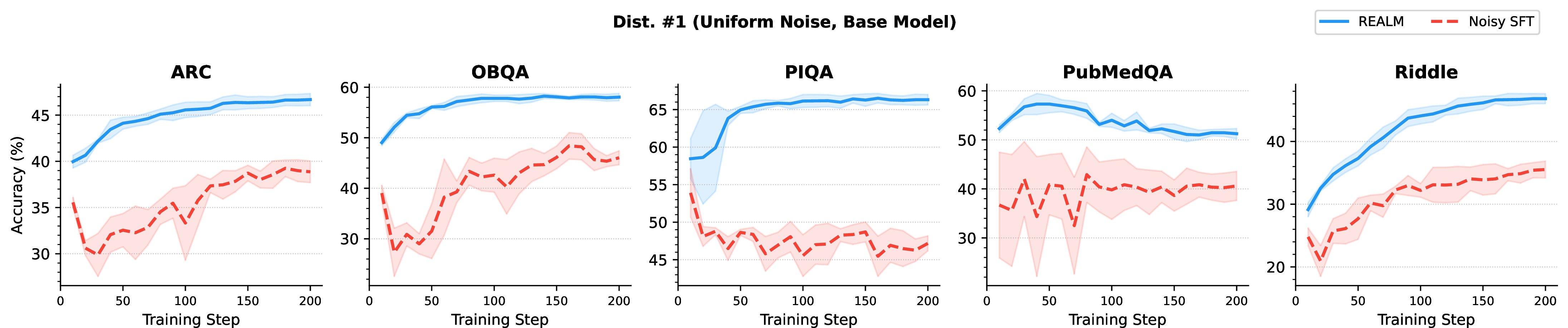
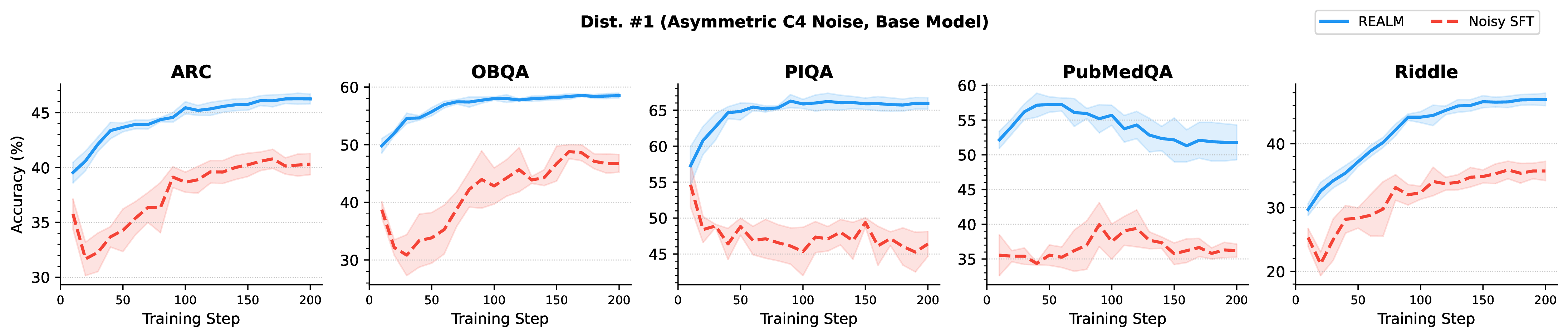
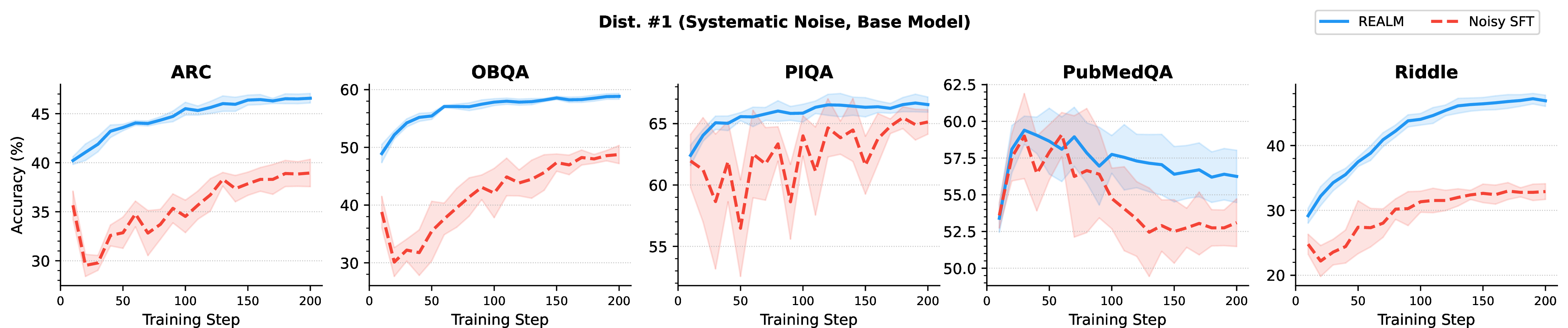
Figure 1: Test accuracy (%) over training steps under Dist. 1⃝ across all three noise types (rows) and five datasets (columns), for the Base model. Shaded bands denote \(\pm\) std over five runs..
4.4 Ablation Study↩︎
Expertise Learning Rate. Table 4 ablates the expertise scalar learning rate \(\eta_\omega\) with the model learning rate fixed at \(5{\times}10^{-5}\). Low values (\(\eta_\omega \leq 0.05\)) cause severe degradation, most notably on PIQA (\(40.91\%\) at \(\eta_\omega{=}0.01\)), because the expertise scalars adapt too slowly to influence training before the model has already absorbed the noise. Performance stabilises at \(\eta_\omega \geq 0.1\) for most datasets, with PIQA requiring \(\eta_\omega{=}0.5\) to fully recover, as the expertise scalars must adapt quickly enough to influence the model before it converges to a noisy solution.
Number of Annotators. Table 5 reports accuracy as the number of annotators grows from \(N{=}3\) to \(N{=}10\) under Dist. . realm outperforms noisy across all datasets and annotator counts, demonstrating that the method scales reliably as the annotator pool grows. As \(N\) increases, annotator expertise values are placed on a uniform grid from \(\beta{=}0.9\) down to \(\beta{=}0.1\), i.e. \(\beta_i = 0.9 - i \cdot \tfrac{0.8}{N-1}\) for \(i = 0, \ldots, N-1\), introducing a larger number of intermediate-reliability annotators with smaller pairwise differences in expertise that are harder to distinguish from one another. This explains the modest drop in average \(\Delta\) from \(+5.93\%\) (\(N{=}3\)) and \(+5.98\%\) (\(N{=}5\)) to \(+5.01\%\) (\(N{=}10\)). Despite this, the gains remain consistent across all annotator counts, confirming that realm is robust to larger annotator pools.
4.5 Learning Curves↩︎
Figure 1 shows test accuracy over training steps under Dist. for all three noise types. Under all three conditions, realm converges smoothly and remains consistently above noisy, while noisy degrades on PIQA as training progresses by absorbing the dominant noise signal from the two unreliable annotators. The separation is most pronounced under asymmetric noise, where noisy collapses more severely, while under systematic noise the gap is smaller but still consistent. Across all noise types, realm exhibits noticeably lower variance than noisy, indicating that jointly learning annotator expertise stabilises training even under distributional mismatch between the noise model and the true label generation process.
5 Conclusion↩︎
We presented REALM, a mixture-based fine-tuning objective that jointly learns language model parameters and per-annotator expertise scalars entirely unsupervised. By modeling each observed label as a convex combination of the model’s prediction and a uniform random guess, REALM automatically identifies and down-weights unreliable annotators without any supervision beyond annotator identity. Experiments on five question answering benchmarks across three model sizes, three noise types, and multiple expertise distributions show that REALM consistently outperforms naive noisy SFT in the large majority of settings, with gains that grow with model capacity and persist even when the noise type violates the model’s generative assumptions. In the multi-task extension, a learned expertise matrix captures per-task annotator reliability and further improves performance across all configurations.
6 Limitations↩︎
Fixed expertise per annotator. REALM assigns a single scalar expertise value to each annotator, constant across all prompts. In practice, an annotator may be reliable on certain question types or domains while performing poorly on others, even within the same dataset. A natural generalisation is to model expertise as a function of the input, \(\rho_i(Q) = \sigma(\langle \boldsymbol{\omega}_i, \phi(Q) \rangle)\), where \(\phi(Q) \in \mathbb{R}^d\) is a learned prompt embedding and \(\boldsymbol{\omega}_i \in \mathbb{R}^d\) is a per-annotator skill vector. This allows expertise to vary continuously across the input space, and subsumes both the single-task scalar (\(d{=}1\)) and the multi-task matrix lookup (when \(\phi(Q)\) is the one-hot task encoding) as special cases. We leave the full exploration of this generalisation to future work.
Multiple-choice tasks. The restricted softmax formulation requires a fixed, discrete set of answer tokens, limiting the current method to multiple-choice tasks. Extending REALM to open-ended generation, where there is no natural \(K\)-class output space, requires a different notion of annotator expertise and a modified mixture objective.
Efficient and Distributed Fine-Tuning. Fine-tuning large language models at scale introduces practical challenges beyond data quality, including communication overhead, privacy constraints, and computational efficiency. In many real-world annotation pipelines, training data is collected from multiple independent sources or organizations, each with its own data distribution and annotation practices, mirroring the federated learning setting where data heterogeneity across clients is a central challenge. Recent work has extended parameter-efficient fine-tuning methods to federated [35] and fully decentralized settings [36], with explicit mechanisms for handling non-i.i.d.data distributions and convergence guarantees. The data heterogeneity problem in these settings is conceptually related to the annotator heterogeneity problem studied in this paper: in both cases, a model must be trained on data from multiple sources of varying quality without access to a unified gold standard. REALM addresses this at the annotation level by learning per-source reliability weights, and combining expertise-aware objectives with federated optimization represents a natural direction for future work.
7 Additional Results↩︎
| Size | Dataset | Oracle | Uniform | Asymmetric | Systematic | ||||||
| realm | noisy | \(\Delta\) | realm | noisy | \(\Delta\) | realm | noisy | \(\Delta\) | |||
| Small | ARC | 29.44 | \(\mathbf{29.05}_{\pm 0.47}\) | \(27.00_{\pm 0.87}\) | \(\mathbf{28.70}_{\pm 0.47}\) | \(27.54_{\pm 0.57}\) | \(\mathbf{28.22}_{\pm 0.90}\) | \(27.43_{\pm 1.21}\) | |||
| OBQA | 44.20 | \(\mathbf{44.28}_{\pm 0.39}\) | \(39.52_{\pm 0.94}\) | \(\mathbf{44.32}_{\pm 0.50}\) | \(40.08_{\pm 0.97}\) | \(\mathbf{43.68}_{\pm 0.92}\) | \(40.00_{\pm 1.67}\) | ||||
| PIQA | 52.88 | \(\mathbf{51.60}_{\pm 1.54}\) | \(51.12_{\pm 0.86}\) | \(50.84_{\pm 1.02}\) | \(\mathbf{51.45}_{\pm 1.35}\) | \(\mathbf{51.32}_{\pm 1.22}\) | \(50.84_{\pm 0.92}\) | ||||
| PubMedQA | 58.00 | \(\mathbf{53.05}_{\pm 1.88}\) | \(50.35_{\pm 3.00}\) | \(\mathbf{50.95}_{\pm 1.90}\) | \(47.05_{\pm 3.75}\) | \(54.90_{\pm 0.96}\) | \(\mathbf{56.50}_{\pm 1.79}\) | ||||
| Riddle | 39.02 | \(\mathbf{34.71}_{\pm 1.14}\) | \(31.25_{\pm 1.11}\) | \(\mathbf{33.49}_{\pm 0.92}\) | \(31.76_{\pm 1.41}\) | \(\mathbf{33.53}_{\pm 0.51}\) | \(30.59_{\pm 1.19}\) | ||||
| Avg | 44.71 | \(\mathbf{42.54}_{\pm 1.08}\) | \(39.85_{\pm 1.36}\) | \(\mathbf{41.66}_{\pm 0.96}\) | \(39.58_{\pm 1.61}\) | \(\mathbf{42.33}_{\pm 0.90}\) | \(41.07_{\pm 1.36}\) | ||||
| Base | ARC | 47.47 | \(\mathbf{45.49}_{\pm 0.80}\) | \(44.31_{\pm 1.01}\) | \(\mathbf{46.11}_{\pm 0.87}\) | \(44.76_{\pm 0.83}\) | \(\mathbf{45.85}_{\pm 0.34}\) | \(44.98_{\pm 0.51}\) | |||
| OBQA | 59.60 | \(\mathbf{58.68}_{\pm 0.81}\) | \(56.84_{\pm 0.64}\) | \(\mathbf{58.24}_{\pm 0.46}\) | \(57.08_{\pm 1.16}\) | \(\mathbf{58.44}_{\pm 0.59}\) | \(56.00_{\pm 0.94}\) | ||||
| PIQA | 67.68 | \(\mathbf{66.55}_{\pm 0.52}\) | \(63.33_{\pm 1.97}\) | \(\mathbf{67.18}_{\pm 0.30}\) | \(63.55_{\pm 1.79}\) | \(\mathbf{66.92}_{\pm 0.42}\) | \(64.87_{\pm 0.97}\) | ||||
| PubMedQA | 61.00 | \(\mathbf{54.00}_{\pm 2.19}\) | \(53.20_{\pm 2.15}\) | \(\mathbf{54.45}_{\pm 1.37}\) | \(51.05_{\pm 1.96}\) | \(56.55_{\pm 1.35}\) | \(\mathbf{60.55}_{\pm 1.26}\) | ||||
| Riddle | 54.12 | \(\mathbf{49.61}_{\pm 1.12}\) | \(45.84_{\pm 1.03}\) | \(\mathbf{49.45}_{\pm 0.91}\) | \(47.92_{\pm 0.76}\) | \(\mathbf{49.25}_{\pm 0.89}\) | \(46.43_{\pm 1.30}\) | ||||
| Avg | 57.97 | \(\mathbf{54.87}_{\pm 1.09}\) | \(52.70_{\pm 1.36}\) | \(\mathbf{55.09}_{\pm 0.78}\) | \(52.87_{\pm 1.30}\) | \(\mathbf{55.40}_{\pm 0.72}\) | \(54.57_{\pm 1.00}\) | ||||
| Large | ARC | 64.81 | \(\mathbf{61.51}_{\pm 0.92}\) | \(57.96_{\pm 0.88}\) | \(\mathbf{62.85}_{\pm 0.92}\) | \(59.09_{\pm 0.85}\) | \(\mathbf{62.40}_{\pm 0.88}\) | \(59.64_{\pm 1.16}\) | |||
| OBQA | 71.60 | \(\mathbf{70.68}_{\pm 0.43}\) | \(68.80_{\pm 0.46}\) | \(\mathbf{70.76}_{\pm 0.70}\) | \(67.40_{\pm 0.88}\) | \(\mathbf{71.00}_{\pm 1.07}\) | \(69.32_{\pm 0.43}\) | ||||
| PIQA | 77.80 | \(\mathbf{77.67}_{\pm 0.64}\) | \(75.10_{\pm 0.23}\) | \(\mathbf{77.37}_{\pm 0.88}\) | \(75.50_{\pm 0.82}\) | \(\mathbf{77.67}_{\pm 0.63}\) | \(75.60_{\pm 1.04}\) | ||||
| PubMedQA | 71.25 | \(\mathbf{60.55}_{\pm 1.93}\) | \(56.00_{\pm 1.15}\) | \(\mathbf{61.50}_{\pm 2.93}\) | \(56.70_{\pm 3.37}\) | \(63.80_{\pm 0.64}\) | \(\mathbf{67.75}_{\pm 1.26}\) | ||||
| Riddle | 67.84 | \(\mathbf{65.45}_{\pm 0.57}\) | \(61.49_{\pm 1.24}\) | \(\mathbf{64.43}_{\pm 0.73}\) | \(62.04_{\pm 1.56}\) | \(\mathbf{65.45}_{\pm 0.73}\) | \(62.75_{\pm 0.57}\) | ||||
| Avg | 70.66 | \(\mathbf{67.17}_{\pm 0.90}\) | \(63.87_{\pm 0.79}\) | \(\mathbf{67.38}_{\pm 1.23}\) | \(64.15_{\pm 1.50}\) | \(\mathbf{68.06}_{\pm 0.79}\) | \(67.01_{\pm 0.89}\) | ||||
| Size | Dataset | Oracle | Uniform | Asymmetric | Systematic | ||||||
| realm | noisy | \(\Delta\) | realm | noisy | \(\Delta\) | realm | noisy | \(\Delta\) | |||
| Small | ARC | 29.44 | \(\mathbf{26.70}_{\pm 0.51}\) | \(26.64_{\pm 1.40}\) | \(27.21_{\pm 0.96}\) | \(\mathbf{27.43}_{\pm 0.96}\) | \(\mathbf{27.45}_{\pm 1.28}\) | \(26.76_{\pm 0.75}\) | |||
| OBQA | 44.20 | \(\mathbf{42.52}_{\pm 0.45}\) | \(35.80_{\pm 2.04}\) | \(\mathbf{42.48}_{\pm 0.82}\) | \(35.76_{\pm 1.88}\) | \(\mathbf{42.56}_{\pm 1.11}\) | \(35.00_{\pm 1.77}\) | ||||
| PIQA | 52.88 | \(\mathbf{52.88}_{\pm 1.18}\) | \(50.36_{\pm 0.60}\) | \(50.25_{\pm 0.87}\) | \(\mathbf{50.58}_{\pm 0.39}\) | \(\mathbf{51.32}_{\pm 1.22}\) | \(50.84_{\pm 0.92}\) | ||||
| PubMedQA | 58.00 | \(\mathbf{50.60}_{\pm 1.97}\) | \(46.55_{\pm 3.17}\) | \(\mathbf{49.00}_{\pm 3.44}\) | \(36.80_{\pm 3.08}\) | \(53.80_{\pm 0.94}\) | \(\mathbf{55.00}_{\pm 0.74}\) | ||||
| Riddle | 39.02 | \(\mathbf{32.16}_{\pm 1.44}\) | \(29.69_{\pm 0.69}\) | \(\mathbf{32.59}_{\pm 1.41}\) | \(29.10_{\pm 0.80}\) | \(\mathbf{32.27}_{\pm 1.14}\) | \(28.16_{\pm 1.64}\) | ||||
| Avg | 44.71 | \(40.97_{\pm 1.11}\) | \(37.81_{\pm 1.58}\) | \(40.31_{\pm 1.50}\) | \(35.93_{\pm 1.42}\) | \(41.48_{\pm 1.14}\) | \(39.15_{\pm 1.16}\) | ||||
| Base | ARC | 47.47 | \(\mathbf{43.78}_{\pm 0.60}\) | \(42.15_{\pm 0.39}\) | \(\mathbf{44.00}_{\pm 0.86}\) | \(42.76_{\pm 1.07}\) | \(\mathbf{43.90}_{\pm 0.47}\) | \(43.52_{\pm 0.68}\) | |||
| OBQA | 59.60 | \(\mathbf{57.96}_{\pm 0.54}\) | \(55.00_{\pm 1.28}\) | \(\mathbf{57.72}_{\pm 1.11}\) | \(55.12_{\pm 0.77}\) | \(\mathbf{58.60}_{\pm 0.95}\) | \(54.36_{\pm 1.24}\) | ||||
| PIQA | 67.68 | \(\mathbf{65.79}_{\pm 0.78}\) | \(51.47_{\pm 1.23}\) | \(\mathbf{65.77}_{\pm 0.71}\) | \(52.10_{\pm 1.75}\) | \(\mathbf{66.92}_{\pm 0.42}\) | \(64.87_{\pm 0.97}\) | ||||
| PubMedQA | 61.00 | \(\mathbf{49.15}_{\pm 1.85}\) | \(44.80_{\pm 3.18}\) | \(\mathbf{52.00}_{\pm 2.42}\) | \(43.70_{\pm 3.32}\) | \(55.85_{\pm 1.93}\) | \(\mathbf{58.45}_{\pm 1.81}\) | ||||
| Riddle | 54.12 | \(\mathbf{46.63}_{\pm 2.01}\) | \(42.00_{\pm 1.88}\) | \(\mathbf{46.94}_{\pm 1.34}\) | \(42.47_{\pm 1.17}\) | \(\mathbf{46.47}_{\pm 1.31}\) | \(42.08_{\pm 0.95}\) | ||||
| Avg | 57.97 | \(52.66_{\pm 1.16}\) | \(47.08_{\pm 1.59}\) | \(53.29_{\pm 1.29}\) | \(47.23_{\pm 1.62}\) | \(54.35_{\pm 1.02}\) | \(52.66_{\pm 1.13}\) | ||||
| Large | ARC | 64.81 | \(\mathbf{59.59}_{\pm 0.64}\) | \(56.14_{\pm 1.07}\) | \(\mathbf{59.64}_{\pm 1.08}\) | \(55.93_{\pm 0.47}\) | \(\mathbf{58.49}_{\pm 0.59}\) | \(56.74_{\pm 0.54}\) | |||
| OBQA | 71.60 | \(\mathbf{70.12}_{\pm 1.24}\) | \(65.68_{\pm 0.52}\) | \(\mathbf{69.80}_{\pm 1.21}\) | \(64.80_{\pm 1.03}\) | \(\mathbf{70.12}_{\pm 1.03}\) | \(65.40_{\pm 1.08}\) | ||||
| PIQA | 77.80 | \(\mathbf{76.50}_{\pm 0.28}\) | \(51.99_{\pm 3.98}\) | \(\mathbf{76.17}_{\pm 0.49}\) | \(53.47_{\pm 2.70}\) | \(\mathbf{77.67}_{\pm 0.63}\) | \(75.60_{\pm 1.04}\) | ||||
| PubMedQA | 71.25 | \(\mathbf{53.45}_{\pm 2.09}\) | \(48.05_{\pm 3.08}\) | \(\mathbf{55.70}_{\pm 2.32}\) | \(47.45_{\pm 2.70}\) | \(60.95_{\pm 2.11}\) | \(\mathbf{64.05}_{\pm 2.85}\) | ||||
| Riddle | 67.84 | \(\mathbf{62.31}_{\pm 1.65}\) | \(57.06_{\pm 2.38}\) | \(\mathbf{61.33}_{\pm 0.96}\) | \(56.16_{\pm 0.98}\) | \(\mathbf{61.25}_{\pm 0.97}\) | \(57.92_{\pm 1.91}\) | ||||
| Avg | 70.66 | \(64.39_{\pm 1.18}\) | \(55.78_{\pm 2.21}\) | \(64.53_{\pm 1.21}\) | \(55.56_{\pm 1.58}\) | \(65.70_{\pm 1.07}\) | \(63.94_{\pm 1.48}\) | ||||
7.1 Results under Dist. 2⃝ and Dist. 3⃝↩︎
Tables 6 and 7 report results under the remaining two expertise distributions. Under Dist. , where two reliable annotators form a majority, gains are modest (avg \(\Delta \leq +4\%\)) since noisy can already exploit the strong majority signal, with PubMedQA reversing under systematic noise at Base and Large model sizes. Under Dist. , gains are larger and asymmetric noise yields the highest average \(\Delta\) across all model sizes, while systematic noise again produces the smallest gains with occasional reversals on PubMedQA. Overall, realm outperforms noisy in the large majority of settings across both distributions, noise types, and model sizes.
7.2 Per-Dataset Multi-Task Results↩︎
Table 8 provides the per-dataset breakdown of the combined multi-task results reported in Table 3. realm outperforms noisy on the large majority of individual dataset and configuration combinations, confirming that the gains observed in the combined accuracy are not driven by a single dataset. The most consistent and largest gains appear on OBQA and Riddle, which have more answer choices (\(K{=}4\) and \(K{=}5\) respectively), giving the mixture objective a stronger signal to discriminate reliable from unreliable annotators. ARC shows smaller but still consistent gains, while a small number of reversals occur on ARC under Dist. #2 for the Small model, where the noise level is low enough that noisy benefits from the larger shared training set.
| Size | Distribution | Dataset | Uniform | Asymmetric | Systematic | |||
| realm | noisy | realm | noisy | realm | noisy | |||
| Small | Dist. | ARC | \(\mathbf{26.35}_{\pm 0.34}\) | \(25.54_{\pm 0.47}\) | \(25.92_{\pm 0.94}\) | \(\mathbf{26.39}_{\pm 0.73}\) | \(\mathbf{26.61}_{\pm 0.86}\) | \(26.05_{\pm 0.21}\) |
| OBQA | \(\mathbf{34.90}_{\pm 0.70}\) | \(29.50_{\pm 1.50}\) | \(\mathbf{34.60}_{\pm 1.40}\) | \(29.50_{\pm 0.50}\) | \(\mathbf{35.80}_{\pm 1.40}\) | \(26.20_{\pm 0.40}\) | ||
| Riddle | \(\mathbf{24.51}_{\pm 1.76}\) | \(20.20_{\pm 0.39}\) | \(\mathbf{24.12}_{\pm 0.59}\) | \(20.29_{\pm 0.10}\) | \(\mathbf{23.33}_{\pm 0.00}\) | \(21.08_{\pm 0.29}\) | ||
| Dist. | ARC | \(26.39_{\pm 0.04}\) | \(\mathbf{27.42}_{\pm 0.04}\) | \(26.78_{\pm 0.09}\) | \(\mathbf{27.77}_{\pm 0.21}\) | \(26.52_{\pm 0.52}\) | \(\mathbf{27.04}_{\pm 0.43}\) | |
| OBQA | \(\mathbf{38.10}_{\pm 1.10}\) | \(36.90_{\pm 0.30}\) | \(\mathbf{37.20}_{\pm 0.80}\) | \(35.40_{\pm 0.40}\) | \(\mathbf{36.20}_{\pm 1.00}\) | \(34.90_{\pm 0.30}\) | ||
| Riddle | \(\mathbf{24.22}_{\pm 0.10}\) | \(22.25_{\pm 0.10}\) | \(\mathbf{24.80}_{\pm 0.10}\) | \(23.92_{\pm 0.20}\) | \(\mathbf{25.00}_{\pm 0.29}\) | \(23.14_{\pm 0.78}\) | ||
| Dist. | ARC | \(26.22_{\pm 0.64}\) | \(\mathbf{26.48}_{\pm 0.39}\) | \(\mathbf{26.35}_{\pm 0.77}\) | \(26.22_{\pm 0.64}\) | \(\mathbf{26.70}_{\pm 0.77}\) | \(26.35_{\pm 0.00}\) | |
| OBQA | \(\mathbf{35.90}_{\pm 1.50}\) | \(33.40_{\pm 2.40}\) | \(\mathbf{34.80}_{\pm 0.80}\) | \(34.60_{\pm 1.20}\) | \(\mathbf{35.50}_{\pm 1.10}\) | \(30.70_{\pm 0.30}\) | ||
| Riddle | \(\mathbf{25.00}_{\pm 0.69}\) | \(20.78_{\pm 0.20}\) | \(\mathbf{25.00}_{\pm 0.10}\) | \(21.37_{\pm 0.00}\) | \(\mathbf{24.31}_{\pm 0.20}\) | \(21.86_{\pm 0.29}\) | ||
| Base | Dist. | ARC | \(\mathbf{41.76}_{\pm 1.07}\) | \(38.67_{\pm 0.90}\) | \(\mathbf{42.15}_{\pm 0.52}\) | \(40.26_{\pm 0.34}\) | \(\mathbf{42.19}_{\pm 0.73}\) | \(38.76_{\pm 0.99}\) |
| OBQA | \(\mathbf{55.00}_{\pm 0.40}\) | \(47.90_{\pm 1.10}\) | \(\mathbf{54.30}_{\pm 0.30}\) | \(45.90_{\pm 0.70}\) | \(\mathbf{54.20}_{\pm 0.20}\) | \(47.70_{\pm 0.10}\) | ||
| Riddle | \(\mathbf{31.57}_{\pm 0.78}\) | \(28.63_{\pm 0.20}\) | \(\mathbf{29.31}_{\pm 0.29}\) | \(26.18_{\pm 0.69}\) | \(\mathbf{29.80}_{\pm 0.98}\) | \(25.69_{\pm 0.20}\) | ||
| Dist. | ARC | \(\mathbf{42.53}_{\pm 0.04}\) | \(41.93_{\pm 0.64}\) | \(\mathbf{42.79}_{\pm 0.30}\) | \(42.19_{\pm 0.30}\) | \(\mathbf{42.32}_{\pm 0.00}\) | \(41.72_{\pm 0.60}\) | |
| OBQA | \(\mathbf{55.50}_{\pm 0.70}\) | \(55.30_{\pm 0.90}\) | \(\mathbf{55.80}_{\pm 0.20}\) | \(53.50_{\pm 1.30}\) | \(\mathbf{54.90}_{\pm 0.30}\) | \(54.80_{\pm 1.60}\) | ||
| Riddle | \(\mathbf{36.37}_{\pm 0.49}\) | \(31.86_{\pm 0.49}\) | \(\mathbf{35.98}_{\pm 0.69}\) | \(32.35_{\pm 0.78}\) | \(\mathbf{35.39}_{\pm 0.69}\) | \(32.94_{\pm 1.76}\) | ||
| Dist. | ARC | \(\mathbf{41.37}_{\pm 0.60}\) | \(40.52_{\pm 0.34}\) | \(\mathbf{42.49}_{\pm 0.26}\) | \(41.50_{\pm 0.47}\) | \(\mathbf{42.49}_{\pm 0.34}\) | \(41.29_{\pm 0.77}\) | |
| OBQA | \(\mathbf{54.90}_{\pm 0.70}\) | \(52.30_{\pm 2.10}\) | \(\mathbf{54.30}_{\pm 0.70}\) | \(53.20_{\pm 0.40}\) | \(\mathbf{55.00}_{\pm 0.00}\) | \(52.80_{\pm 0.40}\) | ||
| Riddle | \(\mathbf{32.94}_{\pm 0.00}\) | \(28.04_{\pm 0.78}\) | \(\mathbf{31.47}_{\pm 0.29}\) | \(28.24_{\pm 0.59}\) | \(\mathbf{31.67}_{\pm 0.29}\) | \(28.53_{\pm 0.69}\) | ||
| Large | Dist. | ARC | \(\mathbf{62.10}_{\pm 0.04}\) | \(58.76_{\pm 0.56}\) | \(\mathbf{61.24}_{\pm 0.21}\) | \(51.89_{\pm 1.59}\) | \(\mathbf{61.67}_{\pm 0.04}\) | \(57.73_{\pm 0.73}\) |
| OBQA | \(\mathbf{68.40}_{\pm 0.20}\) | \(60.90_{\pm 0.90}\) | \(\mathbf{68.10}_{\pm 0.90}\) | \(52.20_{\pm 2.20}\) | \(\mathbf{67.30}_{\pm 1.10}\) | \(61.30_{\pm 0.90}\) | ||
| Riddle | \(\mathbf{52.84}_{\pm 1.47}\) | \(40.20_{\pm 1.96}\) | \(\mathbf{51.08}_{\pm 0.88}\) | \(37.94_{\pm 1.67}\) | \(\mathbf{49.61}_{\pm 0.98}\) | \(37.94_{\pm 1.08}\) | ||
| Dist. | ARC | \(\mathbf{62.06}_{\pm 0.52}\) | \(61.89_{\pm 0.77}\) | \(\mathbf{62.62}_{\pm 0.13}\) | \(61.29_{\pm 0.86}\) | \(\mathbf{62.45}_{\pm 0.04}\) | \(61.03_{\pm 0.09}\) | |
| OBQA | \(\mathbf{69.50}_{\pm 0.30}\) | \(67.80_{\pm 1.20}\) | \(\mathbf{70.40}_{\pm 0.40}\) | \(66.10_{\pm 1.10}\) | \(\mathbf{70.40}_{\pm 0.20}\) | \(67.70_{\pm 0.10}\) | ||
| Riddle | \(\mathbf{56.27}_{\pm 0.39}\) | \(54.41_{\pm 0.88}\) | \(\mathbf{55.20}_{\pm 0.69}\) | \(52.94_{\pm 0.20}\) | \(\mathbf{55.69}_{\pm 0.39}\) | \(54.02_{\pm 0.29}\) | ||
| Dist. | ARC | \(\mathbf{62.83}_{\pm 0.26}\) | \(60.94_{\pm 0.26}\) | \(\mathbf{62.10}_{\pm 0.04}\) | \(58.97_{\pm 0.26}\) | \(\mathbf{61.93}_{\pm 0.04}\) | \(60.82_{\pm 0.04}\) | |
| OBQA | \(\mathbf{69.40}_{\pm 1.00}\) | \(65.20_{\pm 0.40}\) | \(\mathbf{68.70}_{\pm 0.30}\) | \(65.40_{\pm 0.20}\) | \(\mathbf{68.00}_{\pm 0.40}\) | \(65.60_{\pm 1.40}\) | ||
| Riddle | \(\mathbf{54.22}_{\pm 1.08}\) | \(48.92_{\pm 1.47}\) | \(\mathbf{53.73}_{\pm 0.78}\) | \(47.55_{\pm 0.69}\) | \(\mathbf{52.35}_{\pm 0.59}\) | \(46.08_{\pm 1.76}\) | ||