A Sequence-Form Formulation of Logistic Quantal Response Equilibrium in Extensive-Form Games for Selecting Nash Equilibria
April 18, 2026
1 Introduction↩︎
Extensive-form games [1] provide a fundamental framework for modeling sequential strategic interactions in economics, political science, and engineering. Nash equilibrium [2] characterizes strategy profiles from which no player can profitably deviate unilaterally. However, an extensive-form game may possess multiple Nash equilibria, some of which are counterintuitive, thereby limiting the descriptive and predictive power of Nash equilibrium. Logistic QRE, originally introduced by McKelvey and Palfrey[3] for normal-form games, models boundedly rational behavior through payoff-sensitive stochastic choice; when applied to an extensive-form game, it is considered on the game’s associated normal-form representation. As the rationality parameter increases, the limiting Nash equilibrium reached along a continuous QRE branch provides a criterion for equilibrium selection. Logistic QRE satisfies the invariance principle [4], as it is invariant across alternative extensive-form games that induce the same reduced normal form. In contrast, logistic agent QRE [5] is defined by local logit responses at individual information sets and is therefore generally sensitive to the extensive-form structure. These two QRE specifications may therefore induce different QRE paths and select different limiting Nash equilibria. This paper investigates how logistic QRE can be computed in extensive-form games through a sequence-form formulation, thereby enabling the Nash equilibrium selection while avoiding the exponential growth of the normal-form strategy space.
The equilibrium-selection approach associated with logistic QRE admits a natural path-following interpretation [6]. More precisely, the rationality parameter indexes a continuous solution path whose limit points, as the parameter tends to infinity, are Nash equilibria. Path-following methods for computing Nash equilibria in normal-form games have been widely studied. Their early development can be traced back to the Lemke-Howson complementary-pivoting algorithm for bimatrix games [7], which was subsequently generalized to \(n\)-player games by Rosenmüller [8] and Wilson [9]. Subsequent work developed simplicial methods that provided constructive and implementable procedures for computing Nash equilibria in \(n\)-player games [10]–[13]. However, their reliance on increasingly fine simplicial subdivisions may entail substantial computational and storage costs as the dimension of the strategy space grows, thereby limiting their scalability. These limitations motivated the development of differentiable path-following methods. Herings and Peeters [14] introduced the first differentiable path-following method for computing Nash equilibria, based on Harsanyi and Selten’s linear tracing procedure, an early path-based procedure for Nash equilibrium selection. Govindan and Wilson [15] proposed a piecewise-differentiable global Newton method that follows a solution path closely parallel to the linear tracing procedure, while Chen and Dang [16] later attained full differentiability through a modified logarithmic reformulation. Additionally, by exploiting the equilibrium-selection properties embedded in Harsanyi’s tracing procedures and logistic QRE, differentiable methods have also proven effective for the computation of a range of alternative equilibrium concepts [17]–[19].
The sequence form [20]–[22] compactly represents extensive-form games by encoding players’ strategies through action sequences and realization plans. It preserves the sequential structure of the game while scaling linearly in that of the extensive-form game, making it particularly suitable for computing equilibrium concepts defined in the normal form, whose direct treatment is hindered by the exponential growth of the normal-form strategy space. Nash equilibria are conventionally computed in normal-form games. Koller et al. [23] developed an algorithm for computing Nash equilibria of two-player extensive-form games by applying Lemke’s algorithm to the linear complementarity problem induced by the sequence-form representation; the practical efficiency of this approach was demonstrated in the Gala system [24]. For \(n\)-player games, Govindan and Wilson [25] extended structure theorems to perturbed extensive-form games through enabling strategies, which are closely related to sequence-form strategies, and obtained a piecewise-differentiable path-following method for computing Nash equilibria. More recently, Hou et al. [26] developed a globally differentiable sequence-form path-following method for Nash equilibrium computation by incorporating logarithmic-barrier terms into the payoff functions. Computational methods based on the sequence form have also been extended to normal-form equilibrium refinements. Extending the method of van den Elzen and Talman [27] to the extensive-form game, von Stengel et al. [28] established a piecewise linear sequence-form path for computing normal-form perfect equilibria in two-player games. More recently, Hou et al. [29], [30] derived sequence-form characterizations of normal-form perfect and proper equilibria and, on this basis, developed differentiable path-following methods applicable to \(n\)-player games. Related sequence-form methods have also been proposed for equilibrium notions defined through local behavior strategies, including quasi-perfect equilibrium [31], [32], quasi-proper equilibrium [33], and extensive-form perfect equilibrium [34].
Nevertheless, existing sequence-form methods do not directly yield a tractable formulation for the logistic QRE. The challenge lies in representing the payoff-dependent logit responses, which are defined over pure strategies prescribing actions at every information sets, in terms of realization-plan variables that encode only sequence weights. To address this challenge, we construct an entropy-barrier artificial game in the sequence form and establish that its Nash equilibria characterize the logistic QREs of the original extensive-form game. The construction captures the normal-form logit-response structure within the sequence form, thereby circumventing explicit expansion of the exponentially large strategy space. It thereby enables efficient computation of both the logistic QRE path and its limiting equilibrium. We establish its theoretical properties and demonstrate its computational performance through numerical experiments. The remainder of this paper is organized as follows. Section 2 introduces the preliminaries on extensive-form games, logistic QRE, and the sequence form. Section 3 presents the sequence-form formulation of logistic QRE. Section 4 develops a sequence-form differentiable path-following method for tracing the logit-QRE path induced by an arbitrary interior initial point. Section 5 reformulates the dilated-entropy terms in the sequence-form formulation as weighted standard entropy terms, thereby obtaining an equivalent smooth path. Section 6 reports numerical experiments to demonstrate the effectiveness of the proposed method. Section 7 concludes the paper.
2 Preliminaries↩︎
| Symbol | Explanation |
|---|---|
| \(N=\{1,2,\ldots,n\}\) | Set of players |
| \(N_c=N\cup\{c\}\) | Set of players and chance player \(c\) |
| \(a\) | Action taken by a player |
| \(H\) | Set of histories, \(\emptyset\in H\) and \(\langle a_1,\ldots,a_L\rangle\in H\) if \(\langle a_1,\ldots,a_K\rangle\in H\) and \(L<K\) |
| \(Z\) | Set of terminal histories |
| \(A(h)=\{a\mid (h,a)\in H\}\) | Set of actions after a nonterminal history \(h\) |
| \(P(h)\) | Player who takes an action after \(h\) |
| \(f_{c}(a|h)\) | Probability that chance player \(c\) takes action \(a\) after \(h\) |
| \(-i\) | All non-chance players excluding player \(i\in N\) |
| \(\mathcal{I}_{i}\) | Collection of information partitions of \(\{h\in H\mid P(h)=i\}\) |
| \(M_{i}=\{1,\ldots,m_{i}\}\) | Set of information partition indices for player \(i\in N_c\) |
| \(I^{j}_{i}\in\mathcal{I}_{i},j\in M_{i}\) | \(j\)th information set of player \(i\in N_c\), \(A(I^j_i)\triangleq A(h)= A(h')\) whenever \(h,h'\in I^j_i\) |
| \(\succsim_i\) | Preference relation of player \(i\in N\) |
| \(u_z^{i}:Z\to\mathbb{R}\) | Payoff function of player \(i\in N\) |
| \(R_{i}(h)\) | Record of player \(i\in N_c\)’s experience along \(h\) |
| \(|C|\) | Cardinality of a finite set \(C\) |
| \(m_0=\sum_{i\in N}m_i\) | Number of information sets |
| \(n_0=\sum_{i\in N}\sum_{j\in M_i}|A(I^j_i)|\) | Number of actions for non-chance players |
| \(s^i\) | Pure strategy of player \(i\) |
| \(S=\underset{i\in N_c}{\prod}S^i\) | Set of pure-strategy profiles |
| \(u^i(s)\) | Expected payoff of player \(i\) on the pure-strategy profile \(s\in S\) |
| \(\sigma^i\) | Mixed strategy of player \(i\in N_c\), probability measure over \(S^i\) |
| \(\Xi=\underset{i\in N}{\prod}\Xi^i\) | Set of mixed-strategy profiles, \(\Xi^i=\{\sigma^i:S^i\to\mathbb{R}_+\mid \sum\limits_{s^i\in S^i}\sigma^{i}(s^i)=1\}\) |
| \(\Xi_{++}=\underset{i\in N}{\prod} \Xi^i_{++}\) | Set of strictly positive mixed-strategy profiles |
| \(\varpi^i\) | Sequence of actions taken by player \(i\) |
| \(\varpi^i_{I^j_i}\) | Sequence of player \(i\) leading to \(I^j_i\), \(\varpi^i_h=\varpi^i_{I^j_i}\) for any \(h\in I^j_i\) |
| \(\varpi^i_{I^j_i}a\) | The extended sequence \(\varpi^i_{I^j_i}\cup \{a\}\) |
| \({W}=\underset{i\in N_c}\prod{W}^i\) | The collection of sequence profiles, \(\emptyset\in{W}^i\) |
| \(g^i(\varpi)\) | Expected payoff of player \(i\) on the sequence profile \(\varpi\) |
| \(\gamma^i\) | Realization plan of player \(i\in N_c\) |
| \(\Lambda=\underset{i\in N}\prod{ \Lambda^i}\) | Set of realization-plan profiles |
| \(\Lambda_{++}=\underset{i\in N}\prod{ \Lambda^i_{++}}\) | Set of strictly positive realization-plan profiles |
| \(M_i(\varpi^i)\) | The index set of the information sets for player \(i\) with \(\varpi^i\) being the sequence |
| \(m_i(\varpi^i)\) | \(|M_i(\varpi^i)|\) |
Following Osborne and Rubinstein [35], an extensive-form game is represented by \(\Gamma=\langle N, H, P, f_c, \{{\cal I}_i\}_{i\in N}, \{\succsim_i\}_{i\in N}\rangle\), where the notation is summarized in Table 1.Throughout this paper, we consider finite extensive-form games with perfect recall. Finiteness means that the set of histories, \(H\), is finite. Perfect recall requires that, for each player \(i\in N_c\), any two histories \(h\) and \(h'\) belonging to the same information set of player \(i\) satisfy \(R_i(h)=R_i(h')\).
The normal-form representation of \(\Gamma\) is expressed as \(\Gamma_n=\langle N, S, \sigma^c, \{u^i\}_{i\in N}\rangle\), with the associated notation summarized in Table 1. For each player \(i\in N_c\), a pure strategy is a function \(s^i\) that assigns an action in \(A(I_i^j)\) to every information set \(I_i^j\), \(j\in M_i\). Consequently, the number of such pure strategies is \(\prod_{j\in M_i}|A(I_i^j)|\), which grow exponentially in the number of information sets. We instead consider the more compact reduced normal form, in which a pure strategy \(s^i\) prescribes an action at \(I_i^j\) only when that information set is reachable under its preceding prescriptions. Nevertheless, the number of pure strategies in the reduced normal form still grow exponentially with the number of parallel information sets. To facilitate computation, given a pure strategy \(s^i\) of player \(i\in N_c\), let \(s^i(a)\) equal \(1\) if \(s^i\) prescribes action \(a\), and \(0\) otherwise. Then, for any pure-strategy profile \(s=(s^i:i\in N_c)\), the payoff of player \(i\in N\) is give by \(u^i(s)=\sum_{h=\langle a_1,\ldots,a_L\rangle\in Z}u^i_z(h)\prod_{q=0}^{L-1}s^{P(\langle a_1,\ldots,a_q\rangle)}(a_{q+1})\). Given a mixed-strategy profile \(\sigma=(\sigma^i:i\in N)\in \Xi\), the expected payoff of player \(i\in N\) is \(u^i(\sigma)=\sum_{s^i\in S^i}\sigma^i(s^i)u^i(s^i,\sigma^{-i})\) with \(u^i(s^i,\sigma^{-i})=\sum_{s^{-i}\in S^{-i}}u^i(s^i,s^{-i})\prod_{i_q\in N_c\backslash \{i\}}\sigma^{i_q}(s^{i_q})\).
Definition 1. A mixed-strategy profile \(\sigma^*\) is a Nash equilibrium if, for every player \(i\in N\) and \(s^i\in S^i\), it holds that \(\sigma^{*i}(s^i)=0\) whenever \(u^i(s^i,\sigma^{*-i})< u^i(\tilde{s}^i,\sigma^{*-i})\) for some \(\tilde{s}^i\in S^i\).
To accommodate deviations from exact best-response behavior, McKelvey and Palfrey [3] introduced the logistic QRE, which models players’ choices as payoff-sensitive probabilistic responses.
Definition 2. For any given rationality parameter \(\lambda \geq 0\), \(\sigma(\lambda)\in\Xi\) is a logistic QRE if it satisfies \[\label{qrenfne} \sigma^i(\lambda;s^i) = \frac{\exp\left(\lambda u^i(s^i,\sigma^{-i}(\lambda))\right)}{\sum\limits_{s^i_q\in S^i}\exp\left(\lambda u^i(s^i_q,\sigma^{-i}(\lambda))\right)},\; i\in N,s^i\in S^i.\qquad{(1)}\]
To represent the equilibrium-selection process induced by logistic QRE, we introduce an entropy-barrier normal-form game \(\Gamma_n^{e}(t)\), for \(t\in(0,1]\). Each player \(i\) determines an optimal response to a prescribed strategy \(\hat{\sigma}\in\Xi\) by solving the convex optimization problem, \[\label{nfopt:etne} \begin{align} \max\limits_{\sigma^i} & \quad (1-t) \sum\limits_{s^i\in S^i}\sigma^i(s^i) \, u^i(s^i, \hat{\sigma}^{-i})- t \sum\limits_{s^i\in S^i} \sigma^i(s^i) \ln \sigma^i(s^i) \\ \text{s.t.} & \quad \sum\limits_{s^i\in S^i}\sigma^i(s^i) - 1 = 0. \end{align}\tag{1}\] The first-order optimality conditions of 1 , together with the fixed-point condition \(\hat{\sigma}=\sigma\), yield \[\label{nfeqs:etne} \begin{align} & (1-t) u^i(s^i, \sigma^{-i})- t \ln \sigma^i(s^i)- t -\nu^i=0,\; i\in N,s^i\in S^i,\\ & \sum\limits_{s^i\in S^i}\sigma^i(s^i) - 1 = 0,\; i\in N,\;\sigma^i(s^i)>0,\; i\in N,s^i\in S^i. \end{align}\tag{2}\] For \(t\in(0,1]\), define the strictly decreasing function \(\lambda(t)=(1-t)/t\), which satisfies \(\lambda(1)=0\) and \(\lim_{t\to 0^+}\lambda(t)=+\infty\). Then, a mixed-strategy profile \(\sigma\in\Xi\) satisfies the logit-QRE condition in ?? with \(\lambda(t)\) if and only if there exists \(\nu=(\nu^i:i\in N)\) such that \((\sigma,\nu)\) solves System 2 . Consequently, \(\sigma\) is a Nash equilibrium of the entropy-barrier game \(\Gamma_n^{e}(t)\) if and only if it is a logistic QRE of the original game \(\Gamma\). Accordingly, System 2 defines a logit-QRE path that originates from the uniform mixed-strategy profile at \(t=1\) and converges, as \(t\to 0\), to a Nash equilibrium of \(\Gamma\). Nevertheless, the number of variables and constraints in System 2 grows exponentially with the size of the extensive-form game, rendering the computation of this path intractable in general.
Figure 1: 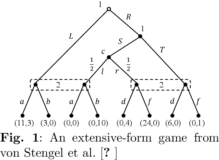 .
.
Figure 2: 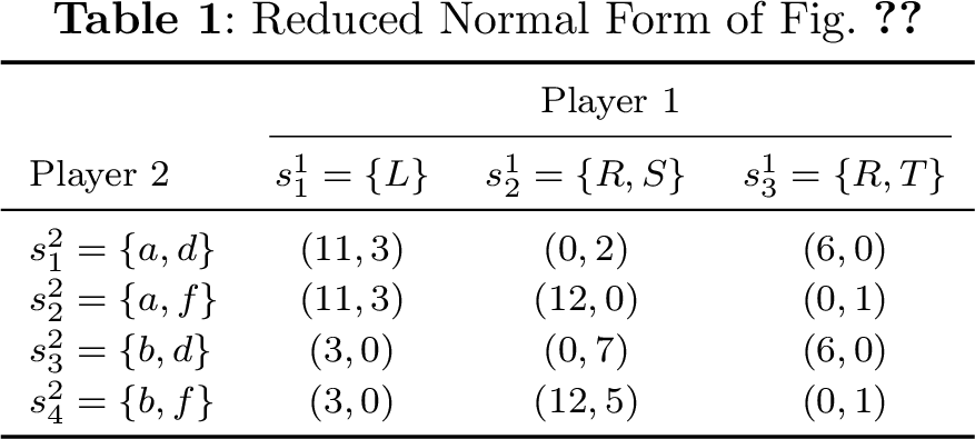 .
.
Example 1.
Consider an extensive-form game \(\Gamma\) shown in Fig. 1, which is the game in Fig. 1 of von Stengel et al. [28]. The players’ information sets are given by \(\mathcal{I}_1=\{I^1_1,I^2_1\}\), \(\mathcal{I}_2=\{I^1_2,I^2_2\}\), and \(\mathcal{I}_c=\{I^1_c\}\), where \(I^1_1=\{\emptyset\}\), \(I^2_1=\{\langle R\rangle\}\), \(I^1_2=\{\langle L\rangle,\langle R,S,l\rangle\}\), \(I^2_2=\{\langle R,S,r\rangle,\langle R,T\rangle\}\), and \(I^1_c=\{\langle R,S\rangle\}\). The pure strategies of the chance player are \(s^c_1=\{l\},s^c_2=\{r\}\). The mixed strategy of the chance player is fixed, given by \(\sigma^c=(\sigma^c(s^c_1),s^c_1(s^c_2))=(0.5,0.5)\). In the normal-form representation, the effect of chance can be incorporated directly into the payoff computation, thereby simplifying the analysis of pure-strategy profiles of the players. The normal-form representation of the extensive-form game can be summarized in Tab. 2. The corresponding mixed strategies are probability measures \(\sigma^1=(\sigma^1(s^1_1),\sigma^1(s^1_2),\sigma^1(s^1_3))^\top\), \(\sigma^2=(\sigma^1(s^2_1),\sigma^1(s^2_2),\sigma^1(s^2_3),\sigma^1(s^2_4))^\top\). Based on Definition 1, the Nash equilibria of the game can be derived manually. This game exhibits three distinct types of Nash equilibria, classified according to their final expected payoffs \(u(\sigma)=(u^1(\sigma),u^2(\sigma))\).
Type A: \(\sigma^1 = (1,0,0)^\top\), \(\sigma^2 = (\sigma^2(s^2_1), 1 - \sigma^2(s^2_1),0,0)^\top\) with \(\frac{1}{12} \le \sigma^2(s^2_1) \le 1\); payoff \(u(\sigma)=(11,3)\).
Type B: \(\sigma^1 = (0,\frac{1}{3},\frac{2}{3})^\top\), \(\sigma^2 = (0,0,\frac{2}{3},\frac{1}{3})^\top\); payoff \(u(\sigma)=(4,\frac{7}{3})\).
Type C: \(\sigma^1 = (\frac{5}{14}, \tfrac{3}{14}, \tfrac{3}{7})^\top\), \(\sigma^2 = (\tfrac{1}{12}, \tfrac{1}{24},\tfrac{7}{12}, \tfrac{7}{24})^\top\); payoff \(u(\sigma)=(4,\frac{3}{2})\).
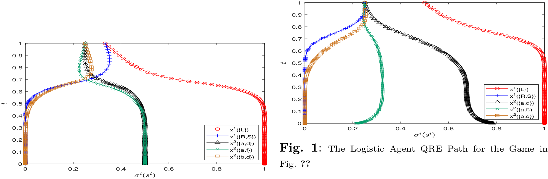
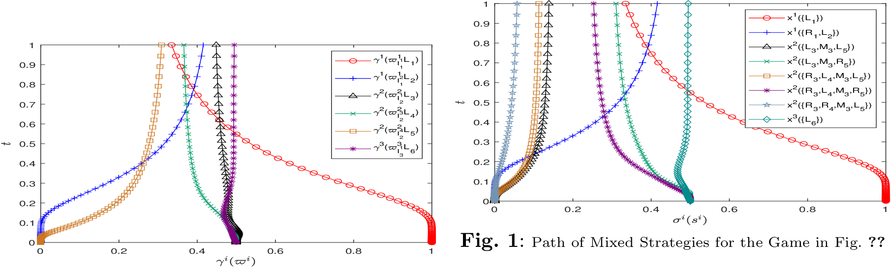
Figs. [Fig02]–3 illustrate that the logistic QRE path and the logistic agent QRE path induce different equilibrium-selection processes and converge to different limiting Nash equilibria of Type A. It should be noted that logistic agent QRE is originally defined in the behavioral-strategy space, where a behavioral strategy assigns probabilities locally to the available actions at each information set. For comparison, we map the logistic agent QRE path to a realization-equivalent mixed-strategy representation. At \(t=1\), where \(\lambda(t)=0\), logistic agent QRE assigns equal probability to the available actions at each information set, generally inducing a mixed-strategy profile different from the uniform initial profile of logistic QRE. Hence, the two paths may start from different points. Even when their initial points are aligned using the generalized construction in Subsection 4, the distinct response mechanisms may still generate different paths and limiting Nash equilibria.
The sequence form, formally developed by von Stengel [22], replaces pure strategies with action sequences and thereby provides a compact representation. The sequence-form representation of \(\Gamma\) is denoted by \(\Gamma_s=\langle N,W,\gamma^c,\{g^i\}_{i\in N}\rangle\) with the relevant notation summarized in Table 1. We say that \(\varpi=(\varpi^i:i\in N_c)\in W\) is induced by a history \(h\in H\) if \(\varpi^i=\varpi_h^i\) for every \(i\in N_c\). For each player \(i\in N\), the payoff function \(g^i\) is defined by \(g^i(\varpi)=u_z^i(h)\) if \(\varpi\) is induced by a terminal history \(h\in Z\), and \(g^i(\varpi)=0\) otherwise. For each player \(i\in N_c\), a realization plan in the sequence form is a function \(\gamma^i\) defined on \({W}^i\) satisfying \(\gamma^i(\emptyset)=1\) and the following flow constraints, \[\label{qre-equ-pre3} \begin{align} & \sum\limits_{a\in A(I_i^j)}\gamma^i(\varpi_{I_i^j}^i a)-\gamma^i(\varpi_{I_i^j}^i)=0,\; j\in M_i,\\ & 0\le \gamma^i(\varpi_{I_i^j}^i a),\; j\in M_i,a\in A(I_i^j). \end{align}\tag{3}\] Given a realization-plan profile \(\gamma=(\gamma^i:i\in N_c)\), the expected payoff of player \(i\in N\) is \(g^i(\gamma)=\sum_{\varpi^i\in W^i}\gamma^i(\varpi^i)g^i(\varpi^i,\gamma^{-i})\), where \(g^i(\varpi^i,\gamma^{-i})=\sum_{\varpi^{-i}\in {W}^{-i}}g^i(\varpi^i,\varpi^{-i})\prod_{i_q\ne i}\gamma^{i_q}(\varpi^{i_q})\). The number of sequences available to player \(i\in N\) is \(\sum_{j \in M_i} |A(I_i^j)|+1\), and hence grows linearly with the number of information sets. The sequence-form representation of the extensive-form game in Fig. 1 is presented in Table 2. The corresponding realization plan satisfies 3 .
| Player 1 Sequences | |||||
|---|---|---|---|---|---|
| 2-6 Player 2 sequences | \(\emptyset\) | \(\varpi^1_{I^1_1}L\) | \(\varpi^1_{I^1_1}R\) | \(\varpi^1_{I^2_1}S\) | \(\varpi^1_{I^2_1}T\) |
| \(\emptyset\) | (0,0) | (0,0) | (0,0) | (0,0) | (0,0) |
| \(\varpi^2_{I^1_2}a\) | (0,0) | (11,3) | (0,0) | (0,0) | (0,0) |
| \(\varpi^2_{I^1_2}b\) | (0,0) | (3,0) | (0,0) | (0,5) | (0,0) |
| \(\varpi^2_{I^2_2}d\) | (0,0) | (0,0) | (0,0) | (0,2) | (6,0) |
| \(\varpi^2_{I^2_2}f\) | (0,0) | (0,0) | (0,0) | (12,0) | (0,1) |
3 A Sequence-Form Formulation of Logistic QRE↩︎
Consider an extensive-form game \(\Gamma\), with \(\Gamma_n\) denoting its normal form and \(\Gamma_s\) its sequence form. Given any pure strategy \(s^i\in S^i\) of player \(i\in N_c\), define \(s^i(\varpi^i)=\prod_{a\in \varpi^i}s^i(a)\) for \(\varpi^i\in W^i\). For any \(\sigma\in \Xi\), let \(\gamma(\sigma)=(\gamma^{i}(\sigma^i;\varpi^i):i\in N_c,\varpi^i\in W^i)\), where \(\gamma^{i}(\sigma^i;\varpi^i)=\sum_{s^i\in S^i}s^i(\varpi^i)\sigma^i(s^i),\,i\in N_c,\varpi^i\in W^i\). It follows that \(\gamma^{i}(s^i;\varpi^i)=s^i(\varpi^i)\) and \(\gamma(\sigma)\in\Lambda\). Define \(T=\left\{(\sigma,\gamma)\left|\sigma\in \Xi,\gamma=\gamma(\sigma)\right.\right\}\), which leads to the following conclusions. For any \(\gamma\in\Lambda\), there exists \(\sigma\in\Xi\) such that \((\sigma,\gamma)\in T\). In particular, for any \(\gamma \in \Lambda_{++}\), one such mixed-strategy profile is given by \(\sigma(\gamma)=(\sigma^i(\gamma^i): i\in N_c)\) with \[\label{gamma2sigma}\sigma^i(\gamma^i;s^i) = \prod_{j\in M_i,\, a\in A(I^j_i),\,s^i(a)=1}\frac{\gamma^i(\varpi^i_{I^j_i}a)}{\gamma^i(\varpi^i_{I^j_i})}.\tag{4}\] Moreover, if \((\sigma,\gamma)\in T\), then \(u^i(\sigma)=g^i(\gamma)\) for every player \(i\in N\). Detailed proofs of these results can be found in Hou et al. [29].
Although multiple mixed-strategy profiles may induce the same realization-plan profile, this cannot occur for distinct logistic QREs: each logistic QRE is uniquely determined by its induced realization plan. The following lemma establishes this property, which provides the basis for formulating logistic QRE directly in the sequence form.
Lemma 1. Let \((\sigma^*,\gamma^*)\in T\). If \(\sigma^*\) is a logistic QRE, then \(\sigma^* = \sigma(\gamma^*)\).
Proof. Fix an arbitrary player \(i\in N\). For any \(\gamma\in\Lambda_{++}\), define recursively \[\label{recurge0} \begin{align} &\mathcal{Z}^i(\gamma;\varpi^i)=\exp\left(\lambda g^i(\varpi^i,\gamma^{-i})\right)\prod\limits_{j\in M_i(\varpi^i)}\mathcal{Z}^i(\gamma;I^j_i),\; \varpi^i\in W^i,\\ &\mathcal{Z}^i(\gamma;I^j_i) = \sum\limits_{a\in A(I^j_i)}\mathcal{Z}^i(\gamma;\varpi^i_{I^j_i}a),\; j\in M_i. \end{align}\tag{5}\] To clarify the proof, for any \(\varpi^i \in W^i\), we define \(s^i_{\varpi^i}\) as a \(\varpi^i\)-partial pure strategy that assigns to each information set along the sequence \(\varpi^i\) the corresponding action \(a \in \varpi^i\), and assigns an action to every information set reachable after \(\varpi^i\). Let \(S^i_{\varpi^i}\) denote the set of all such \(\varpi^i\)-partial pure strategies. In particular, \(S^i_{\varpi^i_\emptyset}=S^i\). By the recursive definition 5 , we obtain \[\label{seqpartpure} \mathcal{Z}^i(\gamma;\varpi^i) = \sum\limits_{s^i_{\varpi^i}\in S^i_{\varpi^i}}\exp\left(\lambda\sum\limits_{\varpi^i_q\in W^i:s^i_{\varpi^i}(\varpi^i_q)=1}g^i(\varpi^i_q,\gamma^{-i})\right).\tag{6}\] Furthermore, it follows from \(u^i(s^i,\sigma^{-i}(\gamma^{-i}))=\sum_{\varpi^i\in W^i:s^i(\varpi^i)=1}g^i(\varpi^i,\gamma^{-i})\) that \(\mathcal{Z}^i(\gamma;\varpi^i_\emptyset) = \sum_{s^i_q\in S_i}\exp\left(\lambda u_i(s^i_q,\sigma^{-i}(\gamma^{-i}))\right)\).
Since \((\sigma^*,\gamma^*)\in T\), the realization plan induced by \(\sigma^{*i}\) satisfies \[\label{eqtransform} \gamma^{*i}(\varpi^i)=\sum_{s^i\in S^i:s^i(\varpi^i)=1}\sigma^{*i}(s^i),\; \varpi^i\in W^i.\tag{7}\] Suppose that \(\sigma^*\) is a logistic QRE with the rationality parameter \(\lambda\). Then, for every \(s^i\in S^i\), we have \[\label{srtqredef} \sigma^{*i}(s^i)=\frac{\exp\left(\lambda u^i(s^i,\sigma^{*-i})\right)}{\sum\limits_{s^i_q\in S^i}\exp\left(\lambda u^i(s^i_q,\sigma^{*-i})\right)}.\tag{8}\] Now consider any information set \(I^j_i\) and any action \(a\in A(I^j_i)\). It follows from 7 and 8 that \[\frac{\gamma^{*i}(\varpi^i_{I^j_i}a)}{\gamma^{*i}(\varpi^i_{I^j_i})} = \frac{\sum\limits_{s^i_q\in S^i:s^i_q(\varpi^i_{I^j_i}a)=1}\exp\left(\lambda u^i(s^i_q,\sigma^{*-i})\right)}{\sum\limits_{s^i_q\in S^i:s^i_q(\varpi^i_{I^j_i})=1}\exp\left(\lambda u^i(s^i_q,\sigma^{*-i})\right)}= \frac{\mathcal{Z}^i(\gamma^{*};\varpi^i_{I^j_i}a)}{\mathcal{Z}^i(\gamma^{*};I^j_i)}.\] The second equality follows from 6 and the fact that \(u^i(s^i_q,\sigma^{*-i})=\sum_{\varpi^i\in W^i:s^i_q(\varpi^i)=1}g^i(\varpi^i,\gamma^{*-i})\) for every \(s^i_q\in S^i\). Building on the preceding results, we next show that \(\sigma^i(\gamma^{*i})\) coincides with \(\sigma^{*i}\). For any \(s^i\in S^i\), we have \[\label{lem1deriveqre} \begin{align} \sigma^i(\gamma^{*i};s^i) & = \prod_{j\in M_i,a\in A(I^j_i): s^i(\varpi^i_{I^j_i}a)=1}\frac{\gamma^{*i}(\varpi^i_{I^j_i}a)}{\gamma^{*i}(\varpi^i_{I^j_i})} = \prod_{j\in M_i, a\in A(I^j_i):s^i(\varpi^i_{I^j_i}a)=1}\frac{\mathcal{Z}^i(\gamma^{*};\varpi^i_{I^j_i}a)}{\mathcal{Z}^i(\gamma^{*};I^j_i)}\\ & =\frac{\exp\left(\lambda \sum\limits_{\varpi^i_q\in W^i:s^i(\varpi^i_q)=1}g^i(\varpi^i_q,\gamma^{*-i})\right)}{\mathcal{Z}^i(,\gamma^{*};\varpi^i_\emptyset)} = \frac{\exp\left(\lambda u^i(s^i,\sigma^{*-i})\right)}{\sum\limits_{s^i_q\in S^i}\exp\left(\lambda u^i(s^i_q,\sigma^{*-i})\right)}=\sigma^{*i}(s^i). \end{align}\tag{9}\] Finally, we conclude that \(\sigma^*=\sigma(\gamma^*)\). This completes the proof. ◻
Using the correspondence in 4 , the entropy term in 1 can be expressed equivalently in terms of realization plans as follows \[\begin{align} \sum\limits_{s^i\in S^i} \sigma^i(\gamma^i;s^i) \ln \sigma^i(\gamma^i;s^i) & = \sum\limits_{j \in M_i} \sum\limits_{a \in A(I_i^j)}\left(\sum\limits_{s^i\in S^i,s^i(\varpi^i_{I_i^j} a)=1} \sigma^i(\gamma^i;s^i)\ln \frac{\gamma^i(\varpi^i_{I^j_i}a)}{\gamma^i(\varpi^i_{I^j_i})}\right)\\ & = \sum\limits_{j \in M_i} \sum\limits_{a \in A(I_i^j)}\gamma^i(\varpi^i_{I^j_i}a)\left(\ln \gamma^i(\varpi^i_{I^j_i}a)-\ln \gamma^i(\varpi^i_{I^j_i})\right). \end{align}\] This gives rise to the dilated-entropy-barrier game \(\Gamma_s^{e}(t)\), in which, given a prescribed realization-plan profile \(\hat{\gamma}\in\Lambda\), each player \(i\) determines an optimal response by solving the following optimization problem \[\label{opt:etne} \begin{align} \max\limits_{\gamma^i} & \quad(1-t) \sum\limits_{j\in M_i} \sum\limits_{a \in A(I_i^j)} \gamma^i(\varpi^i_{I_i^j} a) \, g^i(\varpi^i_{I_i^j} a, \hat{\gamma}^{-i}) \\ & \quad- t \sum\limits_{j \in M_i} \sum\limits_{a \in A(I_i^j)} \gamma^i(\varpi^i_{I_i^j} a) \bigl( \ln \gamma^i(\varpi^i_{I_i^j} a) - \ln \gamma^i(\varpi^i_{I_i^j})\bigr) \\ \text{s.t.} & \quad\sum\limits_{a \in A(I_i^j)} \gamma^i(\varpi^i_{I_i^j} a) - \gamma^i(\varpi^i_{I_i^j}) = 0, \; j \in M_i. \end{align}\tag{10}\] The term “dilated entropy” refers to applying the dilation operation to the standard entropy term associated with each sequence, using the realization weight of its parent sequence as the scaling variable. In accordance with the Nash equilibrium principle, we define \(\gamma^*\) as a Nash equilibrium of \(\Gamma_s^{e}(t)\) precisely when \(\gamma^*\) individually solves Problem 10 against \(\gamma^{*-i}\) for every player \(i\in N\). The preceding construction, together with Lemma 1, establishes the following equivalence.
Theorem 1. Let \((\sigma^*,\gamma^*)\in T\) and \(\sigma^*=\sigma(\gamma^*)\). \(\gamma^*\) is a Nash equilibrium of \(\Gamma_s^{e}(t)\) if and only if \(\sigma^*\) is a logistic QRE with the rationality parameter \(\lambda(t)\).
Applying the first-order stationarity conditions to Problem 10 for each player, and imposing its feasibility constraints together with the equilibrium consistency condition \(\hat{\gamma}=\gamma\), yields the system \[\label{eqt:etnesim}\begin{align} & (1-t)g^i(\varpi^i_{I^j_i}a,\gamma^{-i})-t\bigl( \ln \gamma^i(\varpi^i_{I_i^j} a) - \ln \gamma^i(\varpi^i_{I_i^j})\bigr)\\ & -t(1-m_i(\varpi^i_{I_i^j}a))-\nu^i_{I^j_i} + \zeta^i_{I^j_i}(a) = 0,\;i\in N,j\in M_i,a\in A(I^j_i),\\ & \sum\limits_{a\in A(I^j_i)}\gamma^i(\varpi^i_{I^j_i}a)-\gamma^i(\varpi^i_{I^j_i})=0,\;i\in N,j\in M_i,\;0<\gamma^i(\varpi^i_{I^j_i}a),\;i\in N,j\in M_i,a\in A(I^j_i), \end{align}\tag{11}\] where \(\zeta^i_{I^j_i}(a)=\sum_{{j_q}\in M_i(\varpi^i_{I^j_i}a)}\nu^i_{I^{j_q}_i}\). Because Problem 10 is generally nonconcave, the above first-order derivation establishes only necessity, not sufficiency, with respect to global optimality of Problem 10 . We next prove sufficiency by showing that every solution of System 11 nevertheless induces a logistic QRE.
Theorem 2. If \(\gamma^*\) solves System 11 , then \(\sigma(\gamma^*)\) is a logistic QRE with the rationality parameter \(\lambda(t)\).
Proof. Suppose that \(\gamma^*\) is a Nash equilibrium of \(\Gamma_s^{e}(t)\). From the first group of 11 , we obtain \[\label{eqt:qresf} \frac{\gamma^{*i}(\varpi^i_{I^j_i}a)}{\gamma^{*i}(\varpi^i_{I^j_i})}=\frac{\exp\left(\frac{1-t}{t}g^i(\varpi^i_{I^j_i}a,\gamma^{*-i})+\frac{1}{t}\zeta^i_{I^j_i}(a)+m_i(\varpi^i_{I_i^j}a)\right)}{\exp\left(\frac{1}{t}\nu^i_{I^j_i}+1\right)},\; i\in N,j\in M_i,a\in A(I^j_i).\tag{12}\] We next show, by backward induction, that \[\label{niuvalue} \exp\left(\frac{1}{t}\nu^i_{I^j_i}+1\right) = \mathcal{Z}^i(\gamma^{*};I^j_i), \; i\in N, j\in M_i.\tag{13}\] First, consider \(j\in M_i\) with \((j,a)\in D_i\) for all \(a\in A(I^j_i)\). In this case, 12 implies \[\begin{align} \exp\left(\frac{1}{t}\nu^i_{I^j_i}+1\right) &=\frac{\gamma^{*i}(\varpi^i_{I^j_i})}{\gamma^{*i}(\varpi^i_{I^j_i}a)}\exp\left(\frac{1-t}{t}g^i(\varpi^i_{I^j_i}a,\gamma^{*-i})\right)\\ &= \sum\limits_{a\in A(I^j_i)}\exp\left(\frac{1-t}{t}g^i(\varpi^i_{I^j_i}a,\gamma^{*-i})\right) = \mathcal{Z}^i(\gamma^{*};I^j_i). \end{align}\] Next, consider \(j\in M_i\), and, for any \(a\in A(I^j_i)\) such that \((j,a)\notin D_i\), it holds that \(\exp\big(\frac{1}{t}\nu^i_{I^{j_q}_i}+1\big) = \mathcal{Z}^i(\gamma^{*};I^{j_q}_i)\) for all \(j_q\in M_i(\varpi^i_{I^j_i}a)\). We have \[\begin{align} \exp\left(\frac{1}{t}\nu^i_{I^j_i}+1\right) & =\frac{\gamma^{*i}(\varpi^i_{I^j_i})}{\gamma^{*i}(\varpi^i_{I^j_i}a)}\exp\left(\frac{1-t}{t}g^i(\varpi^i_{I^j_i}a,\gamma^{*-i})\right)\prod\limits_{j_q\in M_i(\varpi^i_{I^j_i}a)}\exp\left(\frac{1}{t}\nu^i_{I^{j_q}_i}+1\right)\\ & = \sum\limits_{a\in A(I^j_i)}\left(\exp\left(\frac{1-t}{t}g^i(\varpi^i_{I^j_i}a,\gamma^{*-i})\right)\prod\limits_{j_q\in M_i(\varpi^i_{I^j_i}a)}\mathcal{Z}^i(\gamma^{*};I^{j_q}_i)\right)= \mathcal{Z}^i(\gamma^{*};I^j_i). \end{align}\] Substituting this identity into 12 yields \[\gamma^{*i}(\varpi^i_{I^j_i}a)=\gamma^{*i}(\varpi^i_{I^j_i})\frac{\mathcal{Z}^i(\gamma^{*};\varpi^i_{I^j_i}a)}{\mathcal{Z}^i(\gamma^{*};I^j_i)},\; i\in N,j\in M_i,a\in A(I^j_i).\] Following the derivation of 9 , we have \[\sigma^i(\gamma^{*i};s^i) = \frac{\exp\left(\lambda(t) u^i(s^i,\sigma^{-i}(\gamma^{*-i}))\right)}{\sum\limits_{s^i_q\in S_i}\exp\left(\lambda(t) u^i(s^i_q,\sigma^{-i}(\gamma^{*-i}))\right)}.\] Consequently, \(\sigma(\gamma^*)\) is a logistic QRE. This completes the proof. ◻
4 Equilibrium Path from an Arbitrary Interior Realization Plan↩︎
4.1 Formulation from an Arbitrary Interior Realization Plan↩︎
Let \(\sigma^0=(\sigma^{0i}(s^i): i\in N, s^i\in S^i)\) be a prescribed totally mixed strategy profile, and let \(\gamma^0=\gamma(\sigma^0)\) be the corresponding realization-plan profile. For any \(\lambda\geq 0\), \(\sigma(\lambda)\in\Xi\) is called a logistic QRE with reference profile \(\sigma^0\) if, for all \(i\in N\) and \(s^i\in S^i\), it satisfies \[\label{qrenfnex0} \sigma^i(\lambda;s^i) = \frac{\sigma^{0i}(s^i)\exp\big(\lambda u^i(s^i,\sigma^{-i}(\lambda))\big)}{\sum\limits_{s^i_q\in S^i}\sigma^{0i}(s^i_q)\exp\big(\lambda u^i(s^i_q,\sigma^{-i}(\lambda))\big)}.\tag{14}\] When \(\lambda=0\), this formulation admits the unique solution \(\sigma(\lambda)=\sigma^0\). In particular, if \(\sigma^{0i}(s^i)=1/|S^i|\) for all \(i\in N\) and \(s^i\in S^i\), then 14 reduces to the standard logistic QRE in Definition 2.
We next construct a corresponding artificial game in the sequence form, denoted by \(\Gamma_s^{e_0}(t)\). In this game, given a prescribed realization-plan profile \(\hat{\gamma}\in\Lambda\), each player \(i\) determines an optimal response by solving the following optimization problem \[\label{opt:etnex0} \begin{align} \max\limits_{\gamma^i} & \quad(1-t) \sum\limits_{j\in M_i} \sum\limits_{a \in A(I_i^j)} \gamma^i(\varpi^i_{I_i^j} a) \, g^i(\varpi^i_{I_i^j} a, \hat{\gamma}^{-i}) \\ & \quad- t \sum\limits_{j \in M_i} \sum\limits_{a \in A(I_i^j)} \gamma^i(\varpi^i_{I_i^j} a) \bigl( \ln \gamma^i(\varpi^i_{I_i^j} a) - \ln \gamma^i(\varpi^i_{I_i^j})-\ln \gamma^{0i}(\varpi^i_{I_i^j} a) + \ln \gamma^{0i}(\varpi^i_{I_i^j})\bigr) \\ \text{s.t.} & \quad\sum\limits_{a \in A(I_i^j)} \gamma^i(\varpi^i_{I_i^j} a) - \gamma^i(\varpi^i_{I_i^j}) = 0, \; j \in M_i. \end{align}\tag{15}\] The second term in the objective function of Problem 15 is a relative dilated-entropy regularizer that penalizes deviations from the reference realization plan \(\gamma^{0i}\). A realization-plan profile \(\gamma^*\) is a Nash equilibrium of \(\Gamma_s^{e_0}(t)\) if, for every player \(i\in N\), \(\gamma^{*i}\) solves Problem 15 with \(\hat{\gamma}^{-i}=\gamma^{*-i}\).
Theorem 3. Let \((\sigma^*,\gamma^*)\in T\) and \(\sigma^*=\sigma(\gamma^*)\). Then \(\gamma^*\) is a Nash equilibrium of \(\Gamma_s^{e_0}(t)\) if and only if \(\sigma^*\) is a logistic QRE defined by 14 with the rationality parameter \(\lambda(t)\).
By combining the first-order stationarity conditions of Problem 15 with its feasibility constraints and the consistency requirement \(\hat{\gamma}=\gamma\), we obtain the following system \[\label{eqt:etnesimx0}\begin{align} & (1-t)g^i(\varpi^i_{I^j_i}a,\gamma^{-i})-t\bigl( \ln \gamma^i(\varpi^i_{I_i^j} a) - \ln \gamma^i(\varpi^i_{I_i^j})-\ln \gamma^{0i}(\varpi^i_{I_i^j} a) + \ln \gamma^{0i}(\varpi^i_{I_i^j})\bigr)\\ & -t(1-m_i(\varpi^i_{I_i^j}a))-\nu^i_{I^j_i} + \zeta^i_{I^j_i}(a) = 0,\;i\in N,j\in M_i,a\in A(I^j_i),\\ & \sum\limits_{a\in A(I^j_i)}\gamma^i(\varpi^i_{I^j_i}a)-\gamma^i(\varpi^i_{I^j_i})=0,\;i\in N,j\in M_i,\;0<\gamma^i(\varpi^i_{I^j_i}a),\;i\in N,j\in M_i,a\in A(I^j_i), \end{align}\tag{16}\] where \(\zeta^i_{I^j_i}(a)=\sum_{{j_q}\in M_i(\varpi^i_{I^j_i}a)}\nu^i_{I^{j_q}_i}\).The following theorem establishes the connection between solutions to System 16 and logistic QREs.
Theorem 4. Any solution \(\gamma^*\) of System 16 induces a logistic QRE \(\sigma(\gamma^*)\) defined by 14 with the rationality parameter \(\lambda(t)\).
It follows from Theorem 4 and 13 that \(\gamma^*\) is a Nash equilibrium of \(\Gamma_s^{e_0}(t)\) if and only if there exists a corresponding multiplier vector \(\nu^*\) such that \((\gamma^*,\nu^*)\) satisfies System 16 .
4.2 Construction of the Selection Path↩︎
In this subsection, we establish the existence of a smooth path consisting of solutions to System (16 ). This path starts from an arbitrary Interior realization plan and ultimately converge into a Nash equilibrium.
Lemma 2. At \(t=1\), System (16 ) has a unique solution, given by \((\gamma^*(1),\nu^*(1))\), with the components satisfying \(\gamma^{*i}(1;\varpi^i_{I^j_i}a)=\gamma^{0i}(\varpi^i_{I^j_i}a)\) and \(\nu^{*i}_{I^j_i}(1)=-1\).
Proof. At \(t=1\), System (16 ) can be expressed as follows, \[\label{nfpe-log-equ-2}\begin{align} & -\bigl( \ln \gamma^i(\varpi^i_{I_i^j} a) - \ln \gamma^i(\varpi^i_{I_i^j})-\ln \gamma^{0i}(\varpi^i_{I_i^j} a) + \ln \gamma^{0i}(\varpi^i_{I_i^j})\bigr)\\ & -(1-m_i(\varpi^i_{I_i^j}a))-\nu^i_{I^j_i} + \zeta^i_{I^j_i}(a) = 0,\;i\in N,j\in M_i,a\in A(I^j_i),\\ & \sum\limits_{a\in A(I^j_i)}\gamma^i(\varpi^i_{I^j_i}a)-\gamma^i(\varpi^i_{I^j_i})=0,\;i\in N,j\in M_i,\; 0<\gamma^i(\varpi^i_{I^j_i}a),\;i\in N,j\in M_i,a\in A(I^j_i), \end{align}\tag{17}\] Suppose that \((\gamma^*(1),\nu^*(1))\) is a solution to System (17 ). Since, there exists a unique logit QRE \(\sigma^*=\sigma^0\) when \(t=1\), it follows from Theorem 3 and 4 that \(\Gamma_s^{e_0}(t)\) has a unique Nash equilibrium \(\gamma^0\). As a result, \(\gamma^*(1)=\gamma^0\). Substituting these results back into the first group of System 17 , it follows that \(\nu^{*i}_{I^j_i}(1) = -1\) for any \(i\in N,j\in M_i\). This completes the proof. ◻
Lemma 2 shows that System (16 ) possesses a unique solution at \(t=1\). In the subsequent discussion, we demonstrate the existence of a connected component that intersects both the \(t=1\) and \(t=0\) levels. Before progressing further, it is essential to introduce Mas-Colell’s fixed-point theorem [36].
Theorem 5. (Mas-Colell’s fixed point theorem). Let \(C\) be a nonempty, compact and convex subset of \(\mathbb{R}^m\) and \(h:C\times[0,1]\to C\) be an upper hemi-continuous mapping. Then the set \(H =\{(z,t)\in C\times[0,1]\mid z=h(z,t)\}\) contains a connected set \(H^c\) such that \(C\times\{1\}\cap H^c\neq\emptyset\) and \(C\times\{0\}\cap H^c\neq\emptyset\).
Let \(\widetilde{\mathscr{S}}_D=\{(\gamma,\nu,t)\mid (\gamma,\nu,t) \text{ satisfies System~(\ref{eqt:etnesimx0}) with } 0<t\leq 1\}\) and \(\mathscr{S}_D\) be the closure of \(\widetilde{\mathscr{S}}_D\). By applying Theorem 5, we arrive at the following conclusion.
Theorem 6. There is a connected component in \(\mathscr{S}_D\) intersecting both \(\mathbb{R}^{n_0}\times\mathbb{R}^{m_0}\times\{1\}\) and \(\mathbb{R}^{n_0}\times\mathbb{R}^{m_0}\times\{0\}\).
Proof. For each \((\hat{\gamma},t)\in \Lambda\times[0,1]\), define the mapping \(\varphi(\hat{\gamma},t)\) as the set of realization-plan profiles \(\gamma=(\gamma^i:i\in N)\) such that, for each player \(i\in N\), \(\gamma^i\) solves Problem 15 when \(t\in (0,1]\), and solves the following optimization problem when \(t=0\) \[\begin{align} \max\limits_{\gamma^i} & \quad\sum\limits_{j\in M_i}\sum\limits_{a\in A(I^j_i)}\gamma^i(\varpi^i_{I^j_i}a)g^i(\varpi^i_{I^j_i}a,\hat{\gamma}^{-i})\\ \text{s.t.} & \quad\sum\limits_{a\in A(I^j_i)}\gamma^i(\varpi^i_{I^j_i}a)-\gamma^i(\varpi^i_{I^j_i})=0,\;j\in M_i. \end{align}\] By Theorem 2.2.2 of Fiacco [37], \(\varphi(\gamma, t)\) is an upper hemi-continuous mapping from \(\Lambda \times [0,1]\) to \(\Lambda\). Let \(\mathscr{E}=\{(\gamma,t)\in\Lambda\times[0,1]\mid\varphi(\gamma,t)=\gamma\}\). Theorem 5 then guarantees the existence of a connected component in \(\mathscr{E}\) that intersects both \(\mathbb{R}^{n_0}\times\{1\}\) and \(\mathbb{R}^{n_0}\times\{0\}\). We denote this component by \(\mathscr{E}^c\), and denote its restriction to \(t>0\) by \(\widetilde{\mathscr{E}}^c\).
For any \((\gamma,t)\in \widetilde{\mathscr{E}}^c\), there exists a unique \(\nu=(\nu^i_{I^j_i}:i\in N,j\in M_i)\) such that System (16 ) is satisfied. Let \(\widetilde{\mathscr{S}}^c_D=\{(\gamma,\nu,t)\in \widetilde{\mathscr{S}}_D\mid(\gamma,t)\in \widetilde{\mathscr{E}}^c\}\) and \(\mathscr{S}^c_D\) be the closure of \(\widetilde{\mathscr{S}}^c_D\). We obtain from the above discussion that \(\mathscr{S}^c_D\) constitutes a connected component within \(\mathscr{S}_D\) intersecting \(\mathbb{R}^{n_0}\times\mathbb{R}^{m_0}\times\{1\}\). Considering a convergent sequence \(\{(\gamma(t_k), t_k)\}^\infty_{k=1} \subseteq \widetilde{\mathscr{E}}^c\) with \(\lim_{k\to\infty} t_k = 0\), we associate each \((\gamma(t_k), t_k)\) with the corresponding \(\nu(t_k)\), which is bounded as shown in Appendix 8. The boundedness of \(\{(\gamma(t_k),\nu(t_k),t_k)\}^\infty_{k=1}\subseteq \widetilde{\mathscr{S}}^c_D\) guarantees that it has a convergent subsequence. Thus, \(\mathscr{S}^c_D\) intersects with \(\mathbb{R}^{n_0}\times\mathbb{R}^{m_0}\times\{0\}\). This completes the proof. ◻
According to Lemma 2, the connected component described in Theorem 6 is unique and intersects the \(t=1\) level at \((\gamma^*(1),\nu^*(1),1)\). Let \(\alpha=(\alpha(\varpi^i_{I^j_i}a):i\in N, j\in M_i, a\in A(I^j_i))\in\mathbb{R}^{n_0}\) be an arbitrary vector with sufficiently small \(\|\alpha\|\). To realize a smooth path, System (16 ) is accordingly modified. Specifically, we subtract the expression \(t(1-t)\alpha\) from the left-hand side of the first group of equations, resulting in a new system. Let \(p(\gamma,\nu,t;\alpha)\) represent the left-hand sides of the equations in the newly obtained system. When treating \(\alpha\) as a constant, we define \(p_\alpha(\gamma,\nu,t) = p(\gamma,\nu,t;\alpha)\). This gives rise to the following theorem.
Theorem 7. Given almost any \(\alpha\in\mathbb{R}^{n_0}\) with sufficiently small \(\|\alpha\|\), there exists a smooth path in \(\mathscr{S}_D\) that starts from \((\gamma^*(1),\nu^*(1),1)\) on the level of \(t=1\) and leads to a Nash equilibrium as \(t\to 0\).
Proof. The second group of equations and inequality constraints in System (16 ) reveals that the elements in \(\mathscr{S}_D\) satisfy \(\gamma\in\text{int}(\Lambda)\) for \(t\in(0,1)\). With the continuous differentiability of \(p(\gamma,\nu,t;\alpha)\) on \(\text{int}(\Lambda)\times\mathbb{R}^{m_0}\times(0,1)\times\mathbb{R}^{n_0}\), we have proved in Appendix 9 that the Jacobian matrix of \(p(\gamma,\nu,t;\alpha)\) is of full-row rank in this region. As an application of the transversality theorem outlined by Eaves and Schmedders [38], it can be shown that zero is a regular value of \(p_\alpha(\gamma,\nu,t)\) over \(\text{int}(\Lambda)\times\mathbb{R}^{m_0}\times(0,1)\) for almost any \(\alpha\). We fix \(\alpha\) such that zero is a regular value of \(p_\alpha(\gamma,\nu,t)\) over \(\text{int}(\Lambda)\times\mathbb{R}^{m_0}\times(0,1)\). By applying the implicit function theorem, the component described in Theorem 6 defines a smooth path, originating at \((\gamma^*(1),\nu^*(1),1)\) when \(t=1\) and terminates at \(t=0\). In Appendix 9, we demonstrate that, at \(t=1\), zero remains a regular value of \(p_\alpha(\gamma,\nu,1)\) in \(\text{int}(\Lambda)\times\mathbb{R}^{m_0}\). This implies that the smooth path does not intersect tangentially with \(\mathbb{R}^{n_0}\times\mathbb{R}^{m_0}\times\{1\}\). By the equilibrium-selection property of logit QRE and Theorem 6, it follows that this smooth path ultimately yields a Nash equilibrium. This completes the proof. ◻
To reformulate System 16 without logarithmic functions, we introduce an exponential transformation on variables in the following. For \(v\in\mathbb{R}\), let \[\phi(v) = \begin{cases} e^{1 - \frac{1}{v}}, & \text{if } v > 0, \\ 0, & \text{if } v \leq 0, \end{cases} \qquad\text{with}\quad \frac{d}{dv} \phi(v) = \begin{cases} \frac{e^{1 - \frac{1}{v}}}{v^2}, & \text{if } v > 0, \\ 0, & \text{if } v \leq 0. \end{cases}\] Clearly, \(\phi(v)\) is continuously differentiable on \(\mathbb{R}\). Furthermore, \(\phi(v)\) is a strictly increasing function on \([0, \infty)\) with \(\phi(1) = 1\). Let \(y=(y^i(\varpi^i_{I^j_i}a):i\in N,j\in M_i,a\in A(I^j_i))\in \mathbb{R}^{n_0}\). We set \(\gamma^i(y;\varpi^i_{I^j_i}a) = \phi(y^i(\varpi^i_{I^j_i}a)), i\in N,j\in M_i,a\in A(I^j_i)\). Substituting \(\gamma(y)=(\gamma^i(y;\varpi^i_{I^j_i}a):i\in N,j\in M_i,a\in A(I^j_i))\) into System (16 ) for \(\gamma\) and subtracting the expression \(t(1-t)\alpha\), we obtain \[\label{eqt:etneexptrans0}\begin{align} & (1-t)g^i(\varpi^i_{I^j_i}a,\gamma^{-i}(y))-t(\ln\gamma^{0i}(\varpi^i_{I^j_i})-\ln\gamma^{0i}(\varpi^i_{I^j_i}a))\\ & +t/y^i(\varpi^i_{I^j_i}a)-t/y^i(\varpi^i_{I^j_i})-t(1-m_i(\varpi^i_{I_i^j}a))-\nu^i_{I^j_i} + \zeta^i_{I^j_i}(a)\\ & -t(1-t)\alpha(\varpi^i_{I^j_i}a) = 0,\;i\in N,j\in M_i,a\in A(I^j_i),\\ & \sum\limits_{a\in A(I^j_i)}\gamma^i(y;\varpi^i_{I^j_i}a)-\gamma^i(y;\varpi^i_{I^j_i})=0,\;i\in N,j\in M_i,\; y^i(\varpi^i_{I^j_i}a)>0,\; i\in N,j\in M_i,a\in A(I^j_i), \end{align}\tag{18}\] where \(y^i(\varpi^i_\emptyset) = 1\). We next introduce two methods for handling fractional terms and inequalities in System 18 , thereby obtaining different transformations that preserve path equivalence.
4.2.0.1 Method 1
We introduce an additional variable transformation as follows. Given \(\kappa_0>1\), let \(\psi_0(v;\kappa_0)=\big((v+\sqrt{v^2})/2\big)^{\kappa_0}\), which is continuously differentiable on \(\mathbb{R}\). For \(x=(x^i(\varpi^i_{I^j_i}a):i\in N,j\in M_i,a\in A(I^j_i))\in \mathbb{R}^{n_0}\), we define \(y(x)=(y^i(x;\varpi^i_{I^j_i}a):i\in N,j\in M_i,a\in A(I^j_i))\) with \(y^i(x;\varpi^i_{I^j_i}a)=\psi_0(x^i(\varpi^i_{I^j_i}a);\kappa_0),\,i\in N,j\in M_i,a\in A(I^j_i)\). Multiplying each equation in the first block of System 18 by its corresponding factor \(y^i(\varpi^i_{I^j_i}a)y^i(\varpi^i_{I^j_i})\), and subsequently replacing \(y\) with \(y(x)\), yields the following equivalent system \[\label{eqt:etneexptrans02}\begin{align} & y^i(x;\varpi^i_{I^j_i}a)y^i(x;\varpi^i_{I^j_i})\Bigl((1-t)g^i(\varpi^i_{I^j_i}a,\gamma^{-i}(y(x)))-t(\ln\gamma^{0i}(\varpi^i_{I^j_i})-\ln\gamma^{0i}(\varpi^i_{I^j_i}a))\\ & -t(1-m_i(\varpi^i_{I_i^j}a))-\nu^i_{I^j_i} + \zeta^i_{I^j_i}(a)-t(1-t)\alpha(\varpi^i_{I^j_i}a) \Bigr)\\ & +t\big(y^i(x;\varpi^i_{I^j_i})-y^i(x;\varpi^i_{I^j_i}a)\big)= 0,\;i\in N,j\in M_i,a\in A(I^j_i),\\ & \sum\limits_{a\in A(I^j_i)}\gamma^i(y(x);\varpi^i_{I^j_i}a)-\gamma^i(y(x);\varpi^i_{I^j_i})=0,\;i\in N,j\in M_i. \end{align}\tag{19}\] At \(t=1\), the system has a unique solution given by \((x^*(1), \nu^*(1))\) with \(x^*(1;\varpi^i_{I^j_i}a)=(1-\ln\gamma^{0i}(\varpi^i_{I^j_i}a))^{1/\kappa_0}\) for \(i\in N,j\in M_i,a\in A(I^j_i)\), and \(\nu^{*i}_{I^j_i}(1) = -1\) for \(i\in N,j\in M_i\).
4.2.0.2 Method 2
Given \(\tau_0>0\) and \(\kappa_0>2\), define \(\psi_1(v,r;\tau_0,\kappa_0)=\big((v+\sqrt{v^2+4\tau_0r})/2\big)^{\kappa_0}\) and \(\psi_2(v,r;\tau_0,\kappa_0)=\big((-v+\sqrt{v^2+4\tau_0r})/2\big)^{\kappa_0}\). It follows that \(\psi_1(v,r;\tau_0,\kappa_0)\psi_2(v,r;\tau_0,\kappa_0)=(\tau_0r)^{\kappa_0}\). Since \(\kappa_0>2\), \(\psi_1(v,r;\tau_0,\kappa_0)\) and \(\psi_2(v,r;\tau_0,\kappa_0)\) are both continuously differentiable on \(\mathbb{R}\times[0,\infty)\). Replacing \(t/y^i(\varpi^i_{I^j_i}a)\) with \(\xi^i(\varpi^i_{I^j_i}a)\) in System 18 , we arrive at an equivalent system. Furthermore, for \(x=(x^i(\varpi^i_{I^j_i}a):i\in N,j\in M_i,a\in A(I^j_i))\in \mathbb{R}^{n_0}\), we define \(y(x,t)=(y^i(x,t;\varpi^i_{I^j_i}a):i\in N,j\in M_i,a\in A(I^j_i))\) and \(\xi(x,t)=(\xi^i(x,t;\varpi^i_{I^j_i}a):i\in N,j\in M_i,a\in A(I^j_i))\), where \(y^i(x,t;\varpi^i_{I^j_i}a)=\psi_1(x^i(\varpi^i_{I^j_i}a),t^{1/\kappa_0}; 1, \kappa_0)\) and \(\xi^i(x,t;\varpi^i_{I^j_i}a)=\psi_2(x^i(\varpi^i_{I^j_i}a),t^{1/\kappa_0};1,\kappa_0),\, i\in N,j\in M_i,a\in A(I^j_i)\). Through the utilization of \(y(x,t)\) and \(\xi(x,t)\), System (18 ) can be equivalently reformulated as \[\label{eqt:etnesqrttrans}\begin{align} & (1-t)g^i(\varpi^i_{I^j_i}a,\gamma^{-i}(y(x,t)))-t(\ln\gamma^{0i}(\varpi^i_{I^j_i})-\ln\gamma^{0i}(\varpi^i_{I^j_i}a))+\xi^i(x,t;\varpi^i_{I^j_i}a)-\xi^i(x,t;\varpi^i_{I^j_i})\\ & -t(1-m_i(\varpi^i_{I_i^j}a))-\nu^i_{I^j_i}+ \zeta^i_{I^j_i}(a)-t(1-t)\alpha(\varpi^i_{I^j_i}a) = 0,\;i\in N,j\in M_i,a\in A(I^j_i),\\ & \sum\limits_{a\in A(I^j_i)}\gamma^i(y(x,t);\varpi^i_{I^j_i}a)-\gamma^i(y(x,t);\varpi^i_{I^j_i})=0,\;i\in N,j\in M_i. \end{align}\tag{20}\] At \(t=1\), the system admits a unique solution \((x^*(1), \nu^*(1))\) given by \(x^{*i}(1;\varpi^i_{I^j_i}a) = (1-\ln\gamma^{0i}(\varpi^i_{I^j_i}a))^{-1/\kappa_0}-(1-\ln\gamma^{0i}(\varpi^i_{I^j_i}a))^{1/\kappa_0}\) for \(i\in N,j\in M_i,a\in A(I^j_i)\), and \(\nu^{*i}_{I^j_i}(1) = -1\) for \(i\in N,j\in M_i\).
5 An Equivalent Smooth Path↩︎
By the constraints 3 , for \(i\in N\) and \(j\in M_i\), we have \(\sum_{a \in A(I_i^j)} \gamma^i(\varpi^i_{I_i^j} a) \big( \ln \gamma^i(\varpi^i_{I_i^j})- \ln \gamma^{0i}(\varpi^i_{I_i^j})\big)=\gamma^i(\varpi^i_{I_i^j} ) \big( \ln \gamma^i(\varpi^i_{I_i^j})- \ln \gamma^{0i}(\varpi^i_{I_i^j})\big)\). Using this identity, the dilated-entropy terms in Problem 15 can be equivalently expressed as a weighted sum of standard entropy terms. Accordingly, Problem 15 can be equivalently rewritten as \[\label{opt:glet} \begin{align} \max\limits_{\gamma^i} &\quad (1-t) \sum\limits_{j\in M_i} \sum\limits_{a \in A(I_i^j)} \gamma^i(\varpi^i_{I_i^j} a) \, g^i(\varpi^i_{I_i^j} a, \hat{\gamma}^{-i}) \\ &\quad- t \sum\limits_{j \in M_i} \sum\limits_{a \in A(I_i^j)} (1-m_i(\varpi^i_{I_i^j}a))\gamma^i(\varpi^i_{I_i^j} a) \bigl( \ln \gamma^i(\varpi^i_{I_i^j} a) - \ln \gamma^{0i}(\varpi^i_{I_i^j} a)\bigr) \\ \text{s.t.} &\quad \sum\limits_{a \in A(I_i^j)} \gamma^i(\varpi^i_{I_i^j} a) - \gamma^i(\varpi^i_{I_i^j}) = 0, \; j \in M_i. \end{align}\tag{21}\] The possible negativity of \(1-m_i(\varpi^i_{I_i^j}a)\) implies that the objective need not be concave. Through the application of the optimality conditions to Problem (21 ) and the fixed-point condition \(\hat{\gamma} = \gamma\), we obtain the following system, \[\label{eqt:glet}\begin{align} & (1-t)g^i(\varpi^i_{I^j_i}a,\gamma^{-i})-t(1-m_i(\varpi^i_{I_i^j}a))\bigl(\ln\gamma^i(\varpi^i_{I^j_i}a)- \ln \gamma^{0i}(\varpi^i_{I_i^j} a)+1\bigr)\\ & -\nu^i_{I^j_i} + \zeta^i_{I^j_i}(a) = 0,\;i\in N,j\in M_i,a\in A(I^j_i),\\ & \sum\limits_{a\in A(I^j_i)}\gamma^i(\varpi^i_{I^j_i}a)-\gamma^i(\varpi^i_{I^j_i})=0,\;i\in N,j\in M_i,\; 0<\gamma^i(\varpi^i_{I^j_i}a),\;i\in N,j\in M_i,a\in A(I^j_i), \end{align}\tag{22}\] where \(\zeta^i_{I^j_i}(a)=\sum_{{j_q}\in M_i(\varpi^i_{I^j_i}a)}\nu^i_{I^{j_q}_i}\). The argument developed in the proof of Theorem 2 extends directly to the present setting, yielding the following result.
Theorem 8. Any solution \(\gamma^*\) of System 22 induces a logistic QRE \(\sigma(\gamma^*)\) defined by 14 with the rationality parameter \(\lambda(t)\).
This result establishes the sufficiency of System 22 for inducing the corresponding logistic QRE. Subtracting \(t(1-t)\alpha\) from the left-hand side of the first group of equations in System 22 yields a new system; let \(\widetilde{\mathscr{S}}_E\) denote the set of all triples \((\gamma,\nu,t)\) satisfying this system for \(0<t\leq1\), and let \(\mathscr{S}_E\) denote its closure. An analogue of Theorem 7 holds: for almost every \(\alpha\in\mathbb{R}^{n_0}\) with sufficiently small \(\|\alpha\|\), there exists a smooth path in \(\mathscr{S}_E\) that originates from \((\gamma^*(1),\nu^*(1),1)\) at \(t=1\), as given in Lemma 2, and converges to a Nash equilibrium as \(t\to0\).
We next treat the logarithmic terms in 22 following an approach analogous to that used in the preceding subsection. Define \(Q_i=\{(j,a)\mid j\in M_i,a\in A(I^j_i),m_i(\varpi^i_{I^j_i}a)\neq 1\}\) for each \(i\in N\). We set \(\gamma^i(y;\varpi^i_{I^j_i}a) = \phi(y^i(\varpi^i_{I^j_i}a))\) for \(i\in N,(j,a)\in Q_i\), and \(\gamma^i(y;\varpi^i_{I^j_i}a) = y^i(\varpi^i_{I^j_i}a)\) for \(i\in N,(j,a)\notin Q_i\). Substituting \(\gamma(y)=(\gamma^i(y;\varpi^i_{I^j_i}a):i\in N,j\in M_i,a\in A(I^j_i))\) for \(\gamma\) in System (22 ) and subtracting the perturbation term \(t(1-t)\alpha\), we obtain \[\label{eqt:gletexptrans0}\begin{align} & (1-t)g^i(\varpi^i_{I^j_i}a,\gamma^{-i}(y))-t(1-m_i(\varpi^i_{I_i^j}a))\bigl(2-\ln\gamma^{0i}(\varpi^i_{I^j_i}a)-1/y^i(\varpi^i_{I^j_i}a)\bigr)\\ & -\nu^i_{I^j_i}+ \zeta^i_{I^j_i}(a)-t(1-t)\alpha(\varpi^i_{I^j_i}a) = 0,\;i\in N,(j,a)\in Q_i,\\ & (1-t)g^i(\varpi^i_{I^j_i}a,\gamma^{-i}(y))-\nu^i_{I^j_i}+ \zeta^i_{I^j_i}(a)-t(1-t)\alpha(\varpi^i_{I^j_i}a) = 0,\;i\in N,(j,a)\notin Q_i,\\ & \sum\limits_{a\in A(I^j_i)}\gamma^i(y;\varpi^i_{I^j_i}a)-\gamma^i(y;\varpi^i_{I^j_i})=0,\;i\in N,j\in M_i,\;y^i(\varpi^i_{I^j_i}a)>0,\; i\in N,(j,a)\in Q_i.\\ \end{align}\tag{23}\] Applying the approach used in the preceding subsection to the fractional terms and inequalities yields the following derivation.
5.0.0.1 Method 3
For \(x=(x^i(\varpi^i_{I^j_i}a):i\in N,j\in M_i,a\in A(I^j_i))\in \mathbb{R}^{n_0}\), we define \(y(x)=(y^i(x;\varpi^i_{I^j_i}a):i\in N,j\in M_i,a\in A(I^j_i))\) with the components being \(y^i(x;\varpi^i_{I^j_i}a)=\psi_0(x^i(\varpi^i_{I^j_i}a);\kappa_0)\) for \(i\in N,(j,a)\in Q_i\) and \(y^i(x;\varpi^i_{I^j_i}a)=x^i(\varpi^i_{I^j_i}a)\) for \(i\in N,(j,a)\notin Q_i\). After multiplying each equation in the first block of System 23 by its associated factor \(y^i(\varpi^i_{I_i^j}a)\) and substituting \(y(x)\) for \(y\), we obtain the following equivalent system \[\label{eqt:etneexptrans12}\begin{align} & y^i(x;\varpi^i_{I^j_i}a)\Bigl((1-t)g^i(\varpi^i_{I^j_i}a,\gamma^{-i}(y(x)))-t(1-m_i(\varpi^i_{I_i^j}a))\bigl(2-\ln\gamma^{0i}(\varpi^i_{I^j_i}a)\bigr)\\ & -\nu^i_{I^j_i}+ \zeta^i_{I^j_i}(a)-t(1-t)\alpha(\varpi^i_{I^j_i}a)\Bigr) + t(1-m_i(\varpi^i_{I_i^j}a))= 0,\;i\in N,(j,a)\in Q_i,\\ & (1-t)g^i(\varpi^i_{I^j_i}a,\gamma^{-i}(y(x)))-\nu^i_{I^j_i}+ \zeta^i_{I^j_i}(a)-t(1-t)\alpha(\varpi^i_{I^j_i}a) = 0,\;i\in N,(j,a)\notin Q_i,\\ & \sum\limits_{a\in A(I^j_i)}\gamma^i(y(x);\varpi^i_{I^j_i}a)-\gamma^i(y(x);\varpi^i_{I^j_i})=0,\;i\in N,j\in M_i.\\ \end{align}\tag{24}\] At \(t=1\), the system has a unique solution given by \((x^*(1), \nu^*(1))\) with \(x^*(1;\varpi^i_{I^j_i}a)=(1-\ln\gamma^{0i}(\varpi^i_{I^j_i}a))^{-1/\kappa_0}\) for \(i\in N,(j,a)\in Q_i\), \(x^*(1;\varpi^i_{I^j_i}a)=\gamma^{0i}(\varpi^i_{I^j_i}a)\) for \(i\in N,(j,a)\notin Q_i\), and \(\nu^{*i}_{I^j_i}(1) = -1\) for \(i\in N,j\in M_i\).
5.0.0.2 Method 4
By replacing \(t/y^i(\varpi^i_{I^j_i}a)\) with \(\xi^i(\varpi^i_{I^j_i}a)\) for \(i\in N,(j,a)\in Q_i\) in System 18 , we obtain an equivalent system. For \(x=(x^i(\varpi^i_{I^j_i}a):i\in N,j\in M_i,a\in A(I^j_i))\in \mathbb{R}^{n_0}\), define \(y(x,t)=(y^i(x,t;\varpi^i_{I^j_i}a):i\in N,j\in M_i,a\in A(I^j_i))\) and \(\xi(x,t)=(\xi^i(x,t;\varpi^i_{I^j_i}a):i\in N,(j,a)\in Q_i)\), where \(y^i(x,t;\varpi^i_{I^j_i}a)=\psi_1(x^i(\varpi^i_{I^j_i}a),t^{1/\kappa_0}; 1, \kappa_0)\), \(\xi^i(x,t;\varpi^i_{I^j_i}a)=\psi_2(x^i(\varpi^i_{I^j_i}a),t^{1/\kappa_0};1,\kappa_0)\) for \(i\in N,(j,a)\in Q_i\), and \(y^i(x,t;\varpi^i_{I^j_i}a)=x^i(\varpi^i_{I^j_i}a)\) for \(i\in N,(j,a)\notin Q_i\). Accordingly, System 23 can be written equivalently as follows \[\label{eqt:gletsqrttrans}\begin{align} & (1-t)g^i(\varpi^i_{I^j_i}a,\gamma^{-i}(y(x,t)))-t(1-m_i(\varpi^i_{I_i^j}a))\bigl(2-\ln\gamma^{0i}(\varpi^i_{I^j_i}a)\bigr)-\nu^i_{I^j_i}+ \zeta^i_{I^j_i}(a)\\ & +(1-m_i(\varpi^i_{I_i^j}a))\xi^i(x,t;\varpi^i_{I^j_i}a)-t(1-t)\alpha(\varpi^i_{I^j_i}a) = 0,\;i\in N,j\in M_i,a\in A(I^j_i),\\ & \sum\limits_{a\in A(I^j_i)}\gamma^i(y(x,t);\varpi^i_{I^j_i}a)-\gamma^i(y(x,t);\varpi^i_{I^j_i})=0,\;i\in N,j\in M_i. \end{align}\tag{25}\] At \(t=1\), System 25 admits a unique solution \((x^*(1), \nu^*(1))\) given by \(x^{*i}(1;\varpi^i_{I^j_i}a) = (1-\ln\gamma^{0i}(\varpi^i_{I^j_i}a))^{-1/\kappa_0}-(1-\ln\gamma^{0i}(\varpi^i_{I^j_i}a))^{1/\kappa_0}\) for \(i\in N,(j,a)\in Q_i\), \(x^{*i}(1;\varpi^i_{I^j_i}a) = \gamma^{0i}(\varpi^i_{I^j_i}a)\) for \(i\in N,(j,a)\notin Q_i\), and \(\nu^i_{I^j_i}(1) = -1\) for \(i\in N,j\in M_i\).
6 Numerical Performance↩︎
We evaluate the proposed sequence-form formulation and its associated path-following methods in two respects. First, we apply the methods to classical extensive-form games to illustrate the resulting logit-QRE paths and to explain their equilibrium-selection behavior. Second, we compare the computational performance of the proposed methods on randomly generated extensive-form games. Our numerical experiments consider four formulations, namely, Systems 19 , 20 , 24 , and 25 , which are denoted by QM1, QM2, QM3, and QM4, respectively. For each formulation, we employ the predictor–corrector method to trace its associated solution path numerically. At each continuation step, the predictor generates an initial approximation to the subsequent point on the path, and the corrector then refines this approximation until the corresponding system is satisfied to the prescribed accuracy. For detailed accounts of predictor–corrector methods, see Allgower and Georg [39].
6.1 Illustration of Logit-QRE Paths↩︎
We first apply the proposed path-following methods to classical extensive-form games to illustrate the resulting logit-QRE paths. Although the four methods are based on different underlying systems, they induce the same realization-plan path. We therefore present this common realization-plan path together with the mixed-strategy path obtained from it through the transformation in 4 . The latter reveals the corresponding normal-form logit-QRE path and its limiting equilibrium-selection outcome, whereas the former provides its realization-plan representation.
Example 2.
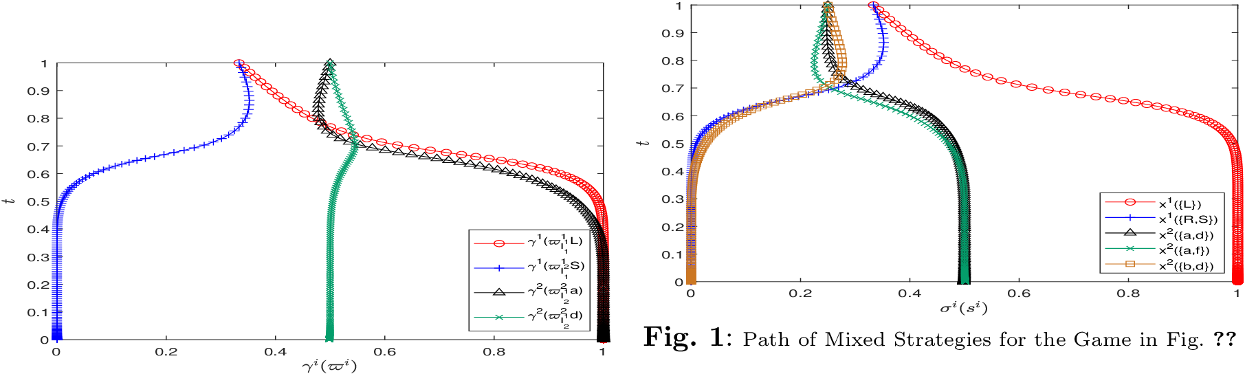
We consider the extensive-form game depicted in Fig. 1 and compare the proposed methods with the path generated by the original normal-form system 2 . For this purpose, the initial mixed-strategy profile is chosen to be uniform, that is, \(\sigma^{0i}(s^i)=1/|S^i|\) for all \(i\in N\) and \(s^i\in S^i\). Figs. [Fig04]–4 present the realization-plan path generated by the proposed methods and its corresponding mixed-strategy path. The latter coincides with the normal-form logit-QRE path in Fig. [Fig02].
Example 3.
We further consider the two multiplayer extensive-form games depicted in Figs. [Fig06] and 5 to demonstrate the proposed formulation. For each game, the initial mixed-strategy profile is randomly drawn from the interior of the corresponding mixed-strategy space. Figs. [Fig08]–7 display the smooth realization-plan paths generated by the proposed methods together with their corresponding paths in mixed-strategy space obtained through the transformation in 4 . As \(t\to 0\), the induced mixed-strategy paths converge to Nash equilibria of the respective games, recovering the limiting equilibria selected along the corresponding normal-form logit-QRE paths.
![Figure 5: An Extensive-Form Game from Selten [40]](/article/2604.16944/_pdflatex/guconbwe.png "fig:")
![Figure 6: Path of Realization Plans for the Game in Fig. [Fig06]](/article/2604.16944/_pdflatex/zqydkalv.png "fig:")
6.2 Computational Comparison of the Proposed Methods↩︎
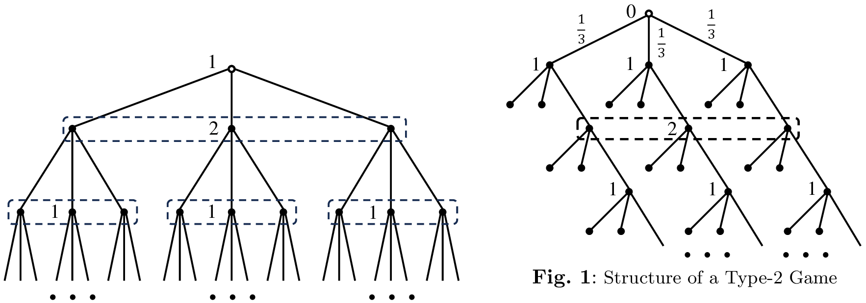
We evaluate the computational performance of QM1–QM4 on randomly generated extensive-form games. The original normal-form system is excluded from the computational comparison because its exponentially growing strategy space rapidly renders direct implementation impractical as game size increases, making the comparison uninformative. Specifically, we consider the two game types illustrated in Figs. [Fig12]–8, which were originally employed in the numerical experiments of [29]. Each game is parameterized by \((n,\mathcal{L},\mathcal{A})\), where \(n\) denotes the number of players, \(\mathcal{L}\) is the maximum history depth, and \(\mathcal{A}\) is the number of available actions at each information set. Players move cyclically along each history, and the payoff of each player at every terminal node is independently drawn from the uniform distribution on \([-10,10]\).
The number of players does not directly determine game size, thus we fixed \(n=3\) for Type 1 games and \(n=4\) for Type 2 games, while varying the remaining two parameters to control game size. For each game type and each parameter configuration \((\mathcal{L},\mathcal{A})\), we generated \(20\) instances with independently sampled payoff specifications. To ensure a fair comparison, all four methods were initialized, for each instance, from the same randomly generated mixed-strategy profile in the interior of the corresponding mixed-strategy space. The predictor step length was initialized as \(t^{0.2}\) and adjusted until the predicted residual satisfied \(0.1t^{0.5}\), while the corrector tolerance was set to \(10^{-16}t^{0.02}\). These settings were held fixed throughout all numerical implementations. A run was deemed successful when the continuation parameter satisfies \(t<10^{-4}\). Conversely, a run was classified as failed when either the prescribed iteration limit or the computational-time limit was exceeded. All computations were conducted on a Windows Server 2016 Standard system equipped with two Intel(R) Xeon(R) E5-2650 v4 processors operating at 2.20 GHz and 128 GB of RAM.
The numerical performance of QM1–QM4 is evaluated in terms of iteration count, computational time, and failure rate. Tables 3–4 report the corresponding results for the two game types. For the first game type, QM1 generally attains the most favorable median iteration counts and computational times. For the second game type, QM3 consistently yields the smallest median iteration counts and computational times while maintaining a zero failure rate throughout. Although QM4 exhibits comparable reliability for this game type, it generally incurs higher iteration counts and computational times than QM3. Overall, the results show that, despite their path equivalence, the four methods differ substantially in numerical efficiency and reliability.
| *\((\mathcal{L},\mathcal{A})\) | |||||||||||||
|---|---|---|---|---|---|---|---|---|---|---|---|---|---|
| (r)7-10(r)11-14 | QM1 | QM2 | QM3 | QM4 | QM1 | QM2 | QM3 | QM4 | QM1 | QM2 | QM3 | QM4 | |
| \((5,2)\) | max | % | % | % | % | ||||||||
| min | |||||||||||||
| med | |||||||||||||
| \((6,2)\) | max | - | - | - | - | - | - | % | % | % | % | ||
| min | |||||||||||||
| med | |||||||||||||
| \((7,2)\) | max | - | - | - | - | - | - | - | - | % | % | % | % |
| min | |||||||||||||
| med | |||||||||||||
| \((8,2)\) | max | - | - | - | - | - | - | - | - | % | % | % | % |
| min | |||||||||||||
| med | - | - | - | - | - | - | |||||||
| \((4,3)\) | max | % | % | % | % | ||||||||
| min | |||||||||||||
| med | |||||||||||||
| \((4,4)\) | max | - | - | - | - | - | - | - | - | % | % | % | % |
| min | |||||||||||||
| med | |||||||||||||
| \((4,5)\) | max | - | - | - | - | - | - | - | - | % | % | % | % |
| min | |||||||||||||
| med |
5pt
| *\((\mathcal{L},\mathcal{A})\) | |||||||||||||
|---|---|---|---|---|---|---|---|---|---|---|---|---|---|
| (r)7-10(r)11-14 | QM1 | QM2 | QM3 | QM4 | QM1 | QM2 | QM3 | QM4 | QM1 | QM2 | QM3 | QM4 | |
| \((20,2)\) | max | % | % | % | % | ||||||||
| min | |||||||||||||
| med | |||||||||||||
| \((30,2)\) | max | - | - | - | - | % | % | % | % | ||||
| min | |||||||||||||
| med | |||||||||||||
| \((40,2)\) | max | - | - | % | % | % | % | ||||||
| min | |||||||||||||
| med | |||||||||||||
| \((50,2)\) | max | - | - | - | - | % | % | % | % | ||||
| min | |||||||||||||
| med | - | - | - | - | |||||||||
| \((10,6)\) | max | - | - | % | % | % | % | ||||||
| min | |||||||||||||
| med | |||||||||||||
| \((10,8)\) | max | % | % | % | % | ||||||||
| min | |||||||||||||
| med | |||||||||||||
| \((10,10)\) | max | % | % | % | % | ||||||||
| min | |||||||||||||
| med | |||||||||||||
| \((10,12)\) | max | - | - | - | - | % | % | % | % | ||||
| min | |||||||||||||
| med | - | - |
5pt
7 Conclusion↩︎
This paper develops sequence-form formulations of logit QRE and differentiable path-following methods for tracing the associated logit-QRE paths in \(n\)-player extensive-form games with perfect recall, thereby efficiently computing the Nash equilibria selected by these paths. We construct a dilated-entropy-barrier artificial game in the sequence form and prove that its Nash equilibria characterize the corresponding logistic QREs, thereby avoiding the exponential growth inherent in the normal-form representation. We further develop a sequence-form formulation of logistic QRE with reference to an arbitrary totally mixed strategy profile, , extending the standard equilibrium-selection process beyond the uniform initial profile. The resulting formulation yields differentiable path-following methods for tracing the associated logit-QRE path and obtaining its selected Nash equilibrium. By rewriting the dilated-entropy terms as the standard entropy terms, we further obtain a path-equivalent formulation and derive additional path-following methods. Numerical experiments illustrate the equilibrium-selection process induced by the proposed methods and evaluate their computational performance. Future work will investigate the use of the proposed sequence-form formulations and path-following methods for the selection of equilibrium refinements.
8 The Boundedness of \(\widetilde{\mathscr{S}}_D\) in Theorem 6↩︎
The objective of this appendix is to elucidate the boundedness of \(\widetilde{\mathscr{S}}_D\), which is necessary for proving Theorem 6.
For any sequence \(\varpi^i\in W^i\), we use \(M_i^+(\varpi^i)\) to denote the index set of all information sets of player \(i\) that may arise after \(\varpi^i\), not necessarily immediately. Let \((\gamma^*,\nu^*,t)\in\mathscr{S}_D\) be a solution of System 16 . Applying backward induction to the first group of equations in System 16 , we obtain, for each \(i\in N\) and \(j\in M_i\), \[\label{app1:recs} \begin{array}{l} -\nu^{*i}_{I^j_i}-1+\sum\limits_{j_q\in M^+_i(\varpi^i_{I^j_i}),a_q\in A(I^{j_q}_i)}\frac{\gamma^{*i}(\varpi^i_{I^{j_q}_i}a_q)}{\gamma^{*i}(\varpi^i_{I^{j}_i})}\biggl((1-t)g^i(\varpi^i_{I^{j_q}_i}a_q,\gamma^{*-i})\\ -t\Bigl( \ln \frac{\gamma^{*i}(\varpi^i_{I^{j_q}_i}a_q)}{\gamma^{*i}(\varpi^i_{I^{j_q}_i})} -\ln\frac{\gamma^{0i}(\varpi^i_{I^{j_q}_i}a_q)}{\gamma^{0i}(\varpi^i_{I^{j_q}_i})}\Bigr)\biggr)=0. \end{array}\tag{26}\] To see this, consider \(i\in N\), \(j\in M_i\) such that \((j,a)\in D_i\) for every \(a\in A(I_i^j)\), 26 follows directly from the first group of equations in System 16 after multiplying them by \(\gamma^{*i}(\varpi^i_{I^{j}_i}a)/\gamma^{*i}(\varpi^i_{I^{j}_i})\) and summing over \(a\in A(I_i^j)\). Now consider the case in which \((j,a)\notin D_i\) for some \(a\in A(I_i^j)\). Suppose that 26 has already been established for every \(j_l\in M_i(\varpi^i_{I_i^j}a)\). Substituting the corresponding identity for \(\zeta^i_{I_i^j}(a)\) into the first group of equations in System 16 gives the desired expression for each \(a\in A(I_i^j)\). Multiplying this expression by \(\gamma^{*i}(\varpi^i_{I^{j}_i}a)/\gamma^{*i}(\varpi^i_{I^{j}_i})\) and summing over \(a\in A(I_i^j)\) gives 26 for \(i\in N\), \(j\in M_i\).
We know that \(-e^{-1}\leq v\ln v\leq 0\) for \(0<v\leq 1\). Let \(U^i_l=\min_{h\in Z}u^i(h)\), \(U^i_u=\max_{h\in Z}u^i(h)\), and \(Y^i_l=\min_{\varpi^i\in W^i}\gamma^{0i}(\varpi^i)\). It then follows from 26 that, for any \(i\in N\) and \(j\in M_i\), \[|W^i|(-|U^i_l|+\ln Y^i_l)-1\leq\nu^{*i}_{I^j_i}\leq |W^i|(|U^i_u|+e^{-1})-1.\]
9 Jacobian Matrix of \(p(\cdot)\) Full-Row Rank Proof in Theorem 7↩︎
This appendix proves that the Jacobian matrix \(Dp(\gamma,\nu,t;\alpha)\) of \(p(\gamma,\nu,t;\alpha)\) has full row rank on \(\text{int}(\Lambda)\times\mathbb{R}^{m_0}\times(0,1)\times\mathbb{R}^{n_0}\), which is critical for the proof of Theorem 7.
Consider the case where \(t\in(0,1)\). We denote the first \(n_0\) terms of \(p(\gamma,\nu,t;\alpha)\) as \(g(\gamma,\nu,t;\alpha)\). The Jacobian matrix \(Dp(\gamma,\nu,t;\alpha)\) is given by \[Dp(\gamma,\nu,t;\alpha)=\left(\begin{array}{cccc} D_{\gamma} g & -B^\top & D_t g & -t(1-t)I^{n_0\times n_0} \\ B & 0 & 0 & 0 \end{array}\right), \nonumber\] where \(I^{n_0\times n_0}\) is an \(n_0\times n_0\) identity matrix, \(B=\bar B-\tilde{B}\), \[\bar B=\left(\begin{array}{cccc} {e^1_1}^\top&&&\\ &{e^2_1}^\top&&\\ &&\ddots&\\ &&&{e^{m_n}_n}^\top \end{array}\right)\in \mathbb{R}^{m_0\times n_0} \text{ with } e^{j}_i=(1,1,\ldots,1)^\top\in\mathbb{R}^{|A(I^j_i)|}. \nonumber\] The matrix \(\tilde{B}\in \mathbb{R}^{m_0\times n_0}\) is defined such that, in each row, the element corresponding to the sequence associated with the relevant information set takes the value \(1\), whereas all remaining elements are set to \(0\). We observe that \(I^{n_0\times n_0}\) and \(B\) are of full-row rank. Thus, for any \(t\in(0,1)\), the Jacobian matrix \(Dp(\gamma,\nu,t;\alpha)\) is of full-row rank.
When \(t=1\), System (16 ) reduces to System (17 ), and the Jacobian matrix takes the block form \[Dp(\gamma,\nu,1;\alpha)=\left(\begin{array}{cc} G & -B^\top \\ B & 0 \end{array}\right). \nonumber\] The block \(G=D_{\gamma} g\) is triangular with diagonal entries \(-1/\gamma^i(\varpi^i_{I^j_i}a),\; i\in N,j\in M_i,a\in A(I^j_i)\). Since \(\gamma\in\Lambda_{++}\), all diagonal entries are nonzero. Hence all eigenvalues of \(G\) are nonzero, and consequently \(G\) is nonsingular. Applying row operations, one can transform \(Dp(\gamma,\nu,1;\alpha)\) to \[Dp(\gamma,\nu,1;\alpha)=\left(\begin{array}{cc} G & -B^\top \\ 0 & BG^{-1}B^\top \end{array}\right). \nonumber\] As \(B\) is of full row rank, \(BG^{-1}B^\top\) is nonsingular. Hence \(Dp(\gamma,\nu,1;\alpha)\) is nonsingular and therefore has full row rank.