1 Introduction↩︎

The Euler beta integral \[\begin{align} \label{Euler-beta} \int_0^1 t^{a - 1} (1 - t)^{b - 1} \, dt= \frac{\Gamma(a) \Gamma(b)}{\Gamma(a + b)}, \qquad \relax a, \relax b > 0, \end{align}\tag{1}\] is one of the simplest integrals that can be expressed in terms of the gamma function \(\Gamma(x)\). The gamma function admits various generalizations depending on additional parameters, see Figure 1. Correspondingly, there are variants of the beta integral, and more generally, of hypergeometric functions, for each type of the gamma function [1].

Various reductions of elliptic hypergeometric functions were considered in  [2]–[4]. Most of them were rigorously proved using the uniform bounds established in [3]. The main goal of the present paper is to prove new limiting relations between hyperbolic and complex rational Euler integrals, which require more refined uniform estimates.

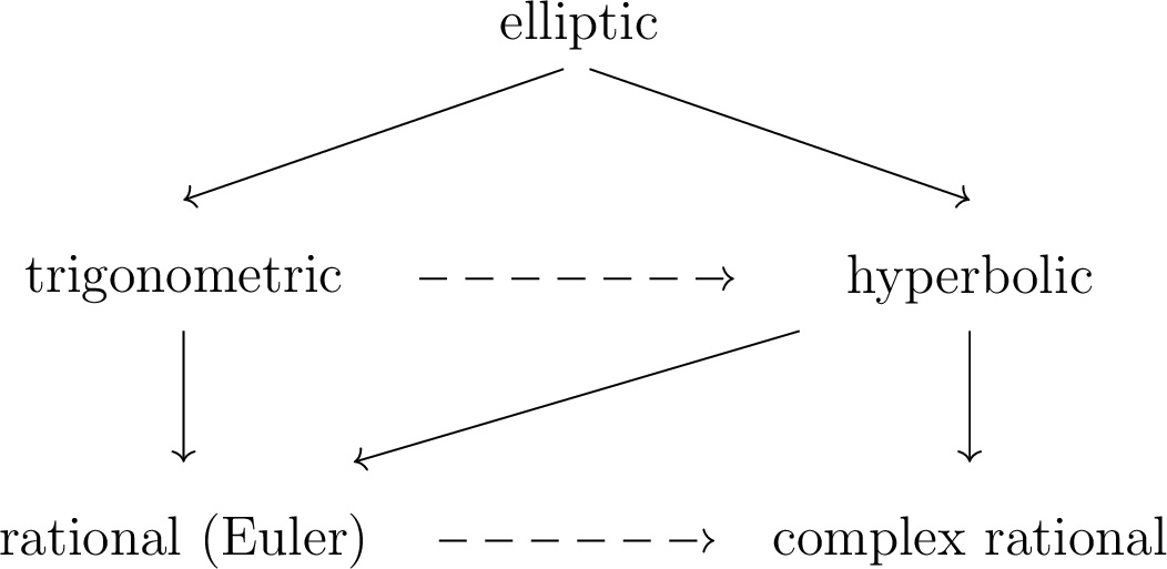
In Section 2 we recall well-known properties of the complex rational and hyperbolic gamma functions, as well as the corresponding beta integrals. Next, in Section 3 we describe the limiting procedure that relates these beta integrals. In Section 4 we show that the prescribed procedure also works for the Euler-type representation of the complex conical function. In Section 5 we outline how the same technique can be applied to the hyperbolic hypergeometric function of Ruijsenaars. In Section 6 we indicate several possible directions for further study. Finally, in the Appendices we prove some uniform bounds for the gamma functions and provide related technical statements.

2 Properties of the gamma functions↩︎

2.1 Complex rational case↩︎

For \(z \in \mathbb{C}\) and a pair \(a, a' \in \mathbb{C}\) denote \[\begin{align} [z]^a = z^a \bar{z}^{a'} = |z|^{a + a'} e^{\mathrm{i}(a - a') \arg z}, \qquad \int_{\mathbb{C}} d^2z = \int_{\mathbb{R}^2} d\relax z \, d \relax z. \end{align}\] The double power \([z]^a\) is a single-valued function of \(z\) if \(a - a' \in \mathbb{Z}\). In all formulas where \(a\) is an explicit integer we set \(a' = a\), for example \([z]^1 = |z|^2\).

For a pair \(a, a' \in \mathbb{C}\) such that \(a - a' \in \mathbb{Z}\) the gamma function associated with the complex field is given by \[\begin{align} \label{cgamma-def} \boldsymbol{\Gamma}(a|a') = \frac{1}{\pi} \int_{\mathbb{C}} [z]^{a - 1} e^{\bar{z} - z} \, d^2z= \frac{\Gamma(a)}{\Gamma(1 - a')}, \end{align}\tag{2}\] see [5]. The integral conditionally converges if \(0 <\relax(a+ a') <1\), while the right-hand side is clearly meromorphic in \(a,a'\in \mathbb{C}\). It satisfies two difference equations \[\begin{align} \boldsymbol{\Gamma}(a + 1|a') = a \boldsymbol{\Gamma}(a|a'), \qquad \boldsymbol{\Gamma}(a|a' + 1) =-a' \boldsymbol{\Gamma}(a|a') \end{align}\] and has the properties \[\begin{align} \boldsymbol{\Gamma}(a|a') = (-1)^{a - a'} \boldsymbol{\Gamma}(a'|a), \qquad \boldsymbol{\Gamma}(a|a') \boldsymbol{\Gamma}(1 - a| 1 - a') = (-1)^{a - a'}, \end{align}\] which follow from the reflection formula \(\Gamma(a) \Gamma(1 - a) = \pi/\sin(\pi a)\).

The complex analogue of the Euler integral 1 has the form \[\begin{align} \label{cgamma-beta} \frac{1}{\pi} \int_{\mathbb{C}} [z]^{a - 1} [1 - z]^{b - 1} d^2z = \frac{\boldsymbol{\Gamma}(a|a') \boldsymbol{\Gamma}(b|b')}{\boldsymbol{\Gamma}(a+b|a'+b')}, \end{align}\tag{3}\] see [6] and references therein. Here we assume \(a - a', b - b' \in \mathbb{Z}\) to have single-valued integrand and \[\begin{align} \relax(a + a') > 0, \qquad \relax(b + b') > 0, \qquad \relax(a + a' + b + b') < 2 \end{align}\] for the integral to be (absolutely) convergent.

2.2 Hyperbolic case↩︎

It is instructive to first recall the trigonometric gamma function due to Jackson \[\begin{align} \label{qgamma} \Gamma_q(z) = \frac{(q; q)_{\infty}}{(q^z; q)_{\infty}} \, (1 - q)^{1 - z}, \qquad (x; q)_{\infty} = \prod_{k = 0}^\infty (1 - xq^{k}), \end{align}\tag{4}\] which satisfies equations \[\begin{align} \Gamma_q(z+1) =\frac{1-q^z}{1-q}\Gamma_q(z), \qquad \Gamma_q\biggl(z+\frac{2\pi \mathrm{i}}{\ln q}\biggr) =e^{-2\pi \mathrm{i}\frac{\ln (1-q)}{\ln q}} \Gamma_q(z). \end{align}\] It reduces to the Euler gamma function in the limit \(\lim_{q \to 1} \Gamma_q(x) = \Gamma(x)\) [7]. The infinite \(q\)-products in 4 converge only if \(|q| < 1\).

The hyperbolic gamma function [8] is a variant of \(q\)-gamma function that remains well defined at \(|q| = 1\). With different conventions it is also known as the “modular quantum dilogarithm” [9] and its reciprocal introduced in [10] is called the “double sine” function. We define it as \[\begin{align} \label{hgamma-def} \gamma^{(2)}(z) \equiv \gamma^{(2)}(z; \omega_1, \omega_2) = e^{- \frac{\pi \mathrm{i}}{2} B_{2,2}(z; \omega_1, \omega_2)} \, \gamma(z; \omega_1, \omega_2) \end{align}\tag{5}\] where \(B_{2,2}\) is the second order multiple Bernoulli polynomial \[\begin{align} \label{B22-def} B_{2,2}(z;\omega_1, \omega_2) = \frac{1}{\omega_1\omega_2} \left( \Bigl(z-\frac{\omega_1+\omega_2}{2} \Bigr)^2-\frac{\omega_1^2+\omega_2^2}{12}\right) \end{align}\tag{6}\] and \[\begin{align} \label{hgamma-int} \gamma(z; \omega_1, \omega_2) = \frac{( \tilde{q} e^{2\pi \mathrm{i}\frac{z}{\omega_1}}; \tilde{q} )_{\infty}}{( e^{2\pi \mathrm{i}\frac{z}{\omega_2}}; q )_{\infty}} = \exp\left(-\int_{\mathbb{R}+\mathrm{i}0}\frac{e^{zt}}{(1-e^{\omega_1 t})(1-e^{\omega_2 t})}\frac{dt}{t}\right) \end{align}\tag{7}\] with parameters \[\begin{align} q = e^{2\pi \mathrm{i}\frac{\omega_1}{\omega_2}}, \qquad \tilde{q} = e^{-2\pi \mathrm{i}\frac{\omega_2}{\omega_1}}. \end{align}\] On the one hand, for \(\relax\omega_1/\omega_2 > 0\) both \(q\)-products in 7 converge and in this case the hyperbolic gamma function is essentially equal to the ratio of two trigonometric ones. This is similar to the relation between rational and complex rational gamma functions. On the other hand, the integral representation 7 is well defined under assumptions \(0 < \relax z < \relax(\omega_1 + \omega_2)\) and \(\relax\omega_1, \relax\omega_2 \geq 0\), which admits \(|q| = |\tilde{q}| = 1\). In what follows we always assume \(\relax\omega_1, \relax\omega_2 \geq 0\).

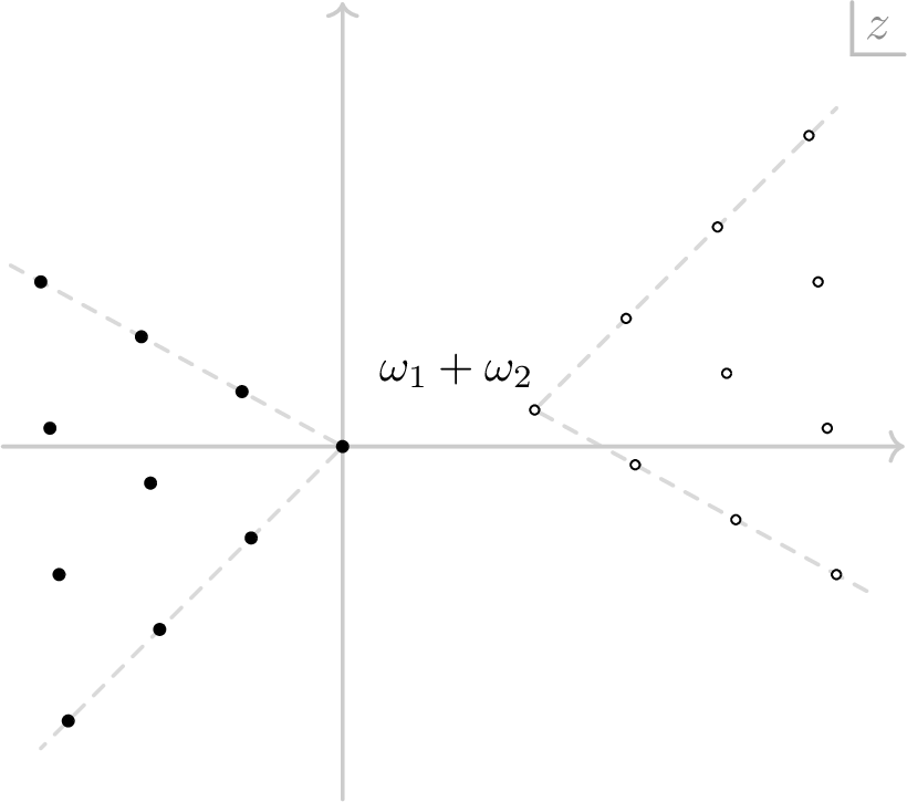
The hyperbolic gamma function satisfies two difference equations \[\begin{align} \frac{\gamma^{(2)}(z + \omega_1) }{\gamma^{(2)}(z)}= 2\sin \frac{\pi z}{\omega_2}, \qquad \frac{\gamma^{(2)}(z + \omega_2)}{\gamma^{(2)}(z)} = 2\sin \frac{\pi z}{\omega_1} \end{align}\] and the reflection relation \[\begin{align} \label{hgamma-refl} \gamma^{(2)}(z) \gamma^{(2)}(\omega_1 + \omega_2 - z) = 1. \end{align}\tag{8}\] As clear from representation 7 , it also has properties \[\begin{align} \gamma^{(2)}(z; \omega_1, \omega_2) = \gamma^{(2)}(z; \omega_2, \omega_1) , \quad \gamma^{(2)}(az; a\omega_1, a\omega_2) = \gamma^{(2)}(z; \omega_1, \omega_2), \quad a> 0 \end{align}\] and it obeys the complex conjugation rule \(\overline{\gamma^{(2)}(z; \omega_1, \omega_2)}=\gamma^{(2)}(\bar z; \bar\omega_1, \bar\omega_2)\). Besides, \(\gamma^{(2)}(z)\) is a meromorphic function with the poles and zeros at the points \[\begin{align} z_{\mathrm{poles}} = - m_1 \omega_1 - m_2 \omega_2, \qquad z_{\mathrm{zeros}} = \omega_1 + \omega_2 + m_1 \omega_1 + m_2 \omega_2, \qquad m_1, m_2 \in \mathbb{Z}_{\geq 0}, \end{align}\] which form two wedges, see Figure 2. Since \(\gamma^{(2)}(z; \omega_1, \omega_2)\) is symmetric in \(\omega_1, \omega_2\), without loss of generality we assume that \(\arg \omega_1 \geq \arg\omega_2\). Then we have the following asymptotics outside of wedges \[\begin{align} \label{hgamma-asymp} \begin{aligned} & \lim_{z\to \infty} e^{\frac{\pi\mathrm{i}}{2} B_{2,2}(z; \omega_1,\omega_2)}\gamma^{(2)}(z)=1, && \quad\arg \omega_1<\arg z<\arg \omega_2+\pi, \\[6pt] & \lim_{z\to \infty} e^{-\frac{\pi\mathrm{i}}{2} B_{2,2}(z; \omega_1,\omega_2)} \gamma^{(2)}(z)=1, && \quad \arg\omega_1-\pi<\arg z<\arg \omega_2. \end{aligned} \end{align}\tag{9}\] Proofs of the above properties can be found in [8], where the function \[\begin{align} \label{G-Ruij} G(\omega_1, \omega_2; z) = \gamma^{(2)}\biggl( \frac{\omega_1 + \omega_2}{2} - \mathrm{i}z; \omega_1, \omega_2 \biggr) \end{align}\tag{10}\] is used.

For brevity, denote \[\begin{align} \gamma^{(2)}(a \pm b) = \gamma^{(2)}(a + b) \, \gamma^{(2)}(a - b). \end{align}\] The hyperbolic gamma function satisfies the Fourier transform identity [11] \[\begin{align} \label{hgamma-beta} \int_{\mathrm{i}\mathbb{R}} e^{\frac{2\pi \mathrm{i}}{\omega_1 \omega_2} \lambda z} \, \gamma^{(2)}\biggl(\pm z + \frac{\omega_1 + \omega_2}{2} - g \biggr) \, \frac{dz}{\mathrm{i}\sqrt{\omega_1 \omega_2}} = \frac{\gamma^{(2)} ( \pm \lambda + g )}{\gamma^{(2)}(2g)}. \end{align}\tag{11}\] Here we assume \(| \relax\lambda| < \relax g < \relax(\omega_1 + \omega_2)/2\): the first inequality ensures convergence, while the second one guarantees that integration contour separates two series of integrand poles.

The above identity is the hyperbolic analogue of Euler beta integral 1 . Indeed, in the limit \(\omega_1 \to 0^+\) (that is \(q \to 1\)) the hyperbolic gamma function reduces to classical functions [8] \[\begin{align} \tag{12} & \gamma^{(2)}(z \omega_1) \underset{\omega_1 \to 0^+}{=} \frac{1}{\sqrt{2\pi}} \, \biggl( \frac{2\pi \omega_1}{\omega_2} \biggr)^{z - \frac{1}{2}} \, \Gamma(z), \\[10pt] \tag{13} & \frac{\gamma^{(2)}(z + u \omega_1)}{\gamma^{(2)}(z)} \underset{\omega_1 \to 0^+}{=} \biggl( 2 \sin \frac{\pi z}{\omega_2} \biggr)^u. \end{align}\] So, assuming \(\omega_1, \omega_2, g > 0\), rescaling the parameters \(g = u \omega_1\), \(\lambda = v \omega_1\) and using reflection formula 8 we obtain \[\begin{align} & \frac{\gamma^{(2)} ( \pm \lambda + g)}{\gamma^{(2)}(2g)} = \frac{\gamma^{(2)} ( (\pm v + u\bigr) \omega_1 )}{\gamma^{(2)}(2u \omega_1)} \underset{\omega_1 \to 0^+}{=} \frac{1}{2\pi} \sqrt{ \frac{\omega_2}{\omega_1} }\, \frac{\Gamma(v + u) \Gamma(-v + u)}{\Gamma(2u)}, \\[10pt] \label{ratio-hgamma-cl-lim} & \gamma^{(2)}\biggl(\pm z + \frac{\omega_1 + \omega_2}{2} - g \biggr) = \frac{\gamma^{(2)}\bigl(z + \frac{\omega_2}{2} + \frac{1 - 2u}{2} \omega_1 \bigr) }{\gamma^{(2)}\bigl(z + \frac{\omega_2}{2} + \frac{1 + 2u}{2} \omega_1 \bigr) } \underset{\omega_1 \to 0^+}{=} \biggl( 2 \cos \frac{\pi z}{\omega_2} \biggr)^{-2u}. \end{align}\tag{14}\] It remains to justify that one can interchange the limit \(\omega_1 \to 0^+\) and integration over \(z\). By [12] we have the bound \[\begin{align} \label{ratio-hgamma-cl-bound} \Biggl| \frac{\gamma^{(2)}\bigl(z + \frac{\omega_2}{2} + \frac{1 - 2u}{2} \omega_1 \bigr) }{\gamma^{(2)}\bigl(z + \frac{\omega_2}{2} + \frac{1 + 2u}{2} \omega_1 \bigr) } \Biggr| \leq C \, e^{-\frac{\pi}{\omega_2} |z|} \end{align}\tag{15}\] uniform in \(z \in \mathrm{i}\mathbb{R}\) and \(\omega_1 \in (0, \Omega]\) for sufficiently small \(\Omega\). Hence, we can use dominated convergence theorem, and the integral identity 11 reduces to \[\begin{align} \label{Euler-beta-2} 2\pi \int_{\mathrm{i}\mathbb{R}} e^{\frac{2\pi \mathrm{i}}{\omega_2} v z} \, \biggl( 2 \cos \frac{\pi z}{\omega_2} \biggr)^{-2u} \, \frac{dz}{\mathrm{i}\omega_2} = \frac{\Gamma(v + u) \Gamma(-v + u)}{\Gamma(2u)}. \end{align}\tag{16}\] This transforms into the Euler integral 1 after the change of variable \(t = 1/(1 + e^{2\pi \mathrm{i}z/\omega_2})\).

3 From hyperbolic to complex rational beta integral↩︎

The reduction described at the end of the previous section is well known. Below we show that the integral 11 can also be reduced to the complex rational beta integral 3 in the limit \(\omega_1/\omega_2 \to -1\) (so that \(q, \tilde{q} \to 1\)).

3.1 Complex limits of the hyperbolic gamma function↩︎

The limit 12 has a complex analogue rigorously derived in [4]. Namely, \[\begin{align} \label{hgamma-comp-lim-1} \gamma^{(2)}(\mathrm{i}\sqrt{\omega_1 \omega_2} [m + u \delta]) \underset{\delta \to 0^+}{=} e^{\frac{\pi \mathrm{i}}{2} m^2} (4\pi \delta)^{\mathrm{i}u - 1} \, \boldsymbol{\Gamma} \biggl( \frac{m + \mathrm{i}u}{2} \bigg| \frac{-m + \mathrm{i}u}{2} \biggr), \end{align}\tag{17}\] where it is assumed that \[\begin{align} \sqrt{ \frac{\omega_1}{\omega_2} } = \mathrm{i}+ \delta + O(\delta^2), \qquad \delta > 0, \qquad m \in \mathbb{Z}, \qquad u \in \mathbb{C}. \end{align}\]

One can apply this limit to the hyperbolic beta integral 11 . It can be done in two different ways. In the first case one can transform the hyperbolic gamma functions in the integrand to the complex gamma functions. In the second situation one takes parameter values such that similar replacement takes place on the right-hand side of 11 . The first limit was described in detail in our recent paper [13] and we briefly recall it here. Denote \[\begin{align} g^* = \frac{\omega_1+\omega_2}{2}-g \end{align}\] and use the following parametrization \[\begin{align} \label{g95bar} g^* = \mathrm{i}\sqrt{\omega_1 \omega_2}(r + h \delta), \qquad \lambda = \mathrm{i}\sqrt{\omega_1 \omega_2} (N+\beta), \qquad r, N \in \mathbb{Z}, \qquad h, \beta \in \mathbb{C}. \end{align}\tag{18}\] When \(\delta\to0^+\) infinite number of poles start to pinch the integration contour around the points \(z \in \mathrm{i}\mathbb{Z}\). Parametrization of \(z\) in the form \[\begin{align} z = \mathrm{i}\sqrt{\omega_1 \omega_2}(m + u \delta), \qquad m \in \mathbb{Z}, \qquad u \in \mathbb{R} \end{align}\] removes pinching and converts the univariate integral over \(z\) into bilateral infinite sum of integrals over the variable \(u\). If one takes \(N = N(\delta)\) in such a way that \(N\delta\to \alpha\) goes to some fixed number, then the exponential factor in the integrand is preserved. The limit on the right-hand side is determined by the following identity established in [13] \[\begin{gather} \label{hgamma-comp-lim-2} e^{-\pi \mathrm{i}Nm - \frac{\pi \mathrm{i}}{2}m^2} \, \frac{ \gamma^{(2)} \bigl(\mathrm{i}\sqrt{\omega_1 \omega_2} [N + \beta + m + u \delta + O(\delta^2)]\bigr) }{ \gamma^{(2)} \bigl(\mathrm{i}\sqrt{\omega_1 \omega_2} [N + \beta]\bigr) } \\ \underset{\substack{\delta \to 0^+\\[2pt] N\delta \to \alpha \;\,}}{=} \bigl(2\mathop{\mathrm{sh}}\pi(\alpha + \mathrm{i}\beta)\bigr)^{\frac{m + \mathrm{i}u}{2}} \, \bigl(2\mathop{\mathrm{sh}}\pi(\alpha - \mathrm{i}\beta)\bigr)^{\frac{-m + \mathrm{i}u}{2}} , \end{gather}\tag{19}\] where it is assumed that¹ \[\begin{align} \sqrt{ \frac{\omega_1}{\omega_2}} = \mathrm{i}+ \delta + O(\delta^2), \qquad \delta > 0, \qquad N, m \in \mathbb{Z}, \qquad u, \beta \in \mathbb{C}. \end{align}\] This is a complex analogue of the limit 13 . As a result, after denoting \(r=2\ell,\, h=2s\), one obtains the following identity \[\begin{align} && \makebox[-2em]{} \frac{1}{4\pi} \sum_{m \in \mathbb{Z}+\mu}\int_{\mathbb{R}} e^{-2\pi \mathrm{i}( \alpha u + \beta m) } \; {\boldsymbol{\Gamma}}(s\pm u,\ell \pm m)\, du \nonumber \\[3pt] && = \boldsymbol{\Gamma}(2s, 2\ell)\bigl( 2 \mathop{\mathrm{ch}}\pi(\alpha + \mathrm{i}\beta) \bigr)^{-\ell - \mathrm{i}s} \bigl( 2 \mathop{\mathrm{ch}}\pi(\alpha - \mathrm{i}\beta) \bigr)^{\ell - \mathrm{i}s}, \label{CBT} \end{align}\tag{20}\] where \(\mu \in \{0, 1/2\}\) is such that \(\ell + m \in \mathbb{Z}\) and the sum of integrals converges for \(\beta \in \mathbb{R}\), \(\relax s>-1/2\). This is the complex binomial theorem which, in turn, is the Fourier inverse of the complex beta integral 3 (cf. 26 , 27 ). For further details, see [13].

The first principal result of the present paper consists in a rigorous proof of the limiting formula in the second possible case, when the univariate integral on the left-hand side of 11 is converted into a two-dimensional integral over the complex plane. For this purpose choose a different parametrization of variables \[\begin{align} \label{gl-param} g = \mathrm{i}\sqrt{\omega_1 \omega_2}(m + u \delta), \qquad \lambda = \mathrm{i}\sqrt{\omega_1 \omega_2}(k + v \delta), \qquad m,k\in \mathbb{Z}, \qquad u, v\in\mathbb{C}, \end{align}\tag{21}\] and apply 17 to the right-hand side of relation 11 , which yields \[\begin{align} \frac{\gamma^{(2)} ( g \pm \lambda)}{\gamma^{(2)}(2g)} \underset{\delta \to 0^+}{=} \frac{e^{\pi \mathrm{i}(m + k)}}{4\pi\delta} \, \frac{\boldsymbol{\Gamma} (a |a') \boldsymbol{\Gamma}(b|b')}{\boldsymbol{\Gamma}(a + b| a' + b')}, \end{align}\] where \[\begin{align} \label{ab-param} \begin{aligned} & a = \frac{m + k + \mathrm{i}(u + v)}{2}, && \qquad a' = \frac{-m - k + \mathrm{i}(u + v)}{2}, \\[6pt] & b = \frac{m - k + \mathrm{i}(u - v)}{2}, && \qquad b' = \frac{- m + k + \mathrm{i}(u - v)}{2}. \end{aligned} \end{align}\tag{22}\] Up to inessential factors the result coincides with the right-hand side of the complex beta integral 3 . Therefore, the same limit should be valid for the left-hand side, that is \[\begin{align} \label{hbeta-lim-1} \lim_{\delta \to 0^+} \delta \, \int_{\mathrm{i}\mathbb{R}} \mathcal{I}(z) \, \frac{dz}{\mathrm{i}\sqrt{\omega_1 \omega_2}} = \frac{e^{\pi \mathrm{i}(m + k)}}{4\pi^2} \int_{\mathbb{C}} [t]^{a - 1} [1 - t]^{b - 1} d^2t , \end{align}\tag{23}\] where \[\begin{align} \label{Id} \mathcal{I}(z) = e^{\frac{2\pi \mathrm{i}}{\omega_1 \omega_2} \lambda z} \, \gamma^{(2)}\biggl(\pm z + \frac{\omega_1 + \omega_2}{2} - g \biggr). \end{align}\tag{24}\] A natural question arises whether this reduction can be performed directly at the level of integrals.

Formula 19 implies that the integrand 24 with \(g, \lambda\) parametrized as in 21 and \(\sqrt{\omega_1/\omega_2} = \mathrm{i}+ \delta + O(\delta^2)\) has the limit \[\begin{gather} \label{Id-lim} \mathcal{I}(\mathrm{i}\sqrt{\omega_1 \omega_2}[N + \beta]) = e^{-2\pi \mathrm{i}(\beta k + (N + \beta) v \delta )} \, \frac{\gamma^{(2)}\bigl(\mathrm{i}\sqrt{\omega_1 \omega_2} [N + \beta - m - (u + \mathrm{i}) \delta + O(\delta^2) ]\bigr)}{ \gamma^{(2)}\bigl(\mathrm{i}\sqrt{\omega_1 \omega_2} [N + \beta + m + (u - \mathrm{i}) \delta + O(\delta^2)] \bigr) } \\[6pt] \underset{\substack{\delta \to 0^+\\[2pt] N\delta \to \alpha \; \,}}{=} \frac{e^{-2\pi \mathrm{i}(\alpha v + \beta k)}}{ (2\mathop{\mathrm{sh}}\pi (\alpha + \mathrm{i}\beta))^{m + \mathrm{i}u} \, (2\mathop{\mathrm{sh}}\pi (\alpha - \mathrm{i}\beta))^{-m + \mathrm{i}u}}, \end{gather}\tag{25}\] where we assume \(N \in \mathbb{Z}\), \(\alpha, \beta \in \mathbb{R}\).

The complex beta integral can also be written in terms of the exponential functions. Changing the integration variable \(t = 1/(1 - e^{2\pi(\alpha + \mathrm{i}\beta)})\) and inserting parametrization 22 we have \[\begin{align} \label{cbeta-exp} \frac{e^{\pi \mathrm{i}(m + k)}}{4\pi^2} \int_{\mathbb{C}} [t]^{a - 1} [1 - t]^{b - 1} d^2t = \int_{\mathbb{R}} d\alpha \int_{-\frac{1}{2}}^{\frac{1}{2}} \mathcal{J}(\alpha, \beta) \, d\beta, \end{align}\tag{26}\] where \[\begin{align} \label{Jd} \mathcal{J}(\alpha, \beta) := \frac{e^{-2\pi \mathrm{i}(\alpha v + \beta k)}}{ (2\mathop{\mathrm{sh}}\pi (\alpha + \mathrm{i}\beta))^{m + \mathrm{i}u} \, (2\mathop{\mathrm{sh}}\pi (\alpha - \mathrm{i}\beta))^{-m + \mathrm{i}u}}. \end{align}\tag{27}\] Notice that \(\mathcal{J}(\alpha, \beta)\) is \(1\)-periodic in \(\beta\), \(\mathcal{J}(\alpha, \beta+1) = \mathcal{J}(\alpha, \beta)\), i.e. one can use for integration over \(\beta\) any interval \([a, a + 1]\). In the above notation the formula 25 simply reads \[\begin{align} \label{Id-lim-2} \mathcal{I}(\mathrm{i}\sqrt{\omega_1 \omega_2}[N + \beta]) \underset{\substack{\delta \to 0^+\\[2pt] N\delta \to \alpha \; \,}}{=} \mathcal{J}(\alpha, \beta), \end{align}\tag{28}\] while the reduction 23 is equivalent to the following statement.

The proof by direct transformation of one integral into another is given in Sections 3.2–3.4. But before that let us make a few remarks about the assumptions on the parameters ?? , ?? . First, notice that \(\sqrt{\omega_1/\omega_2} = \mathrm{i}+ \delta + O(\delta^2)\), as desired. The choice \(\delta=1/n\), \(n\in\mathbb{Z}_{>0}\), is done for a convenience of considerations below.

Second, recall that the hyperbolic beta integral evaluation formula 11 holds under the assumption \(|\relax\lambda| < \relax g < \relax(\omega_1 + \omega_2)/2 = \delta\). To simplify matters, in what follows we take \(\lambda \in \mathrm{i}\mathbb{R}\), or equivalently \(v \in \mathbb{R}\).² Hence, the condition \(0 < \relax g < \delta\) forces the assumption \(\relax u \in (-1, 0)\).

Finally, it is also possible to perform the reduction in the case \(m,k \in \mathbb{Z} + 1/2\). This requires only slight modifications, and we omit it to ease the exposition.

3.2 Outline↩︎

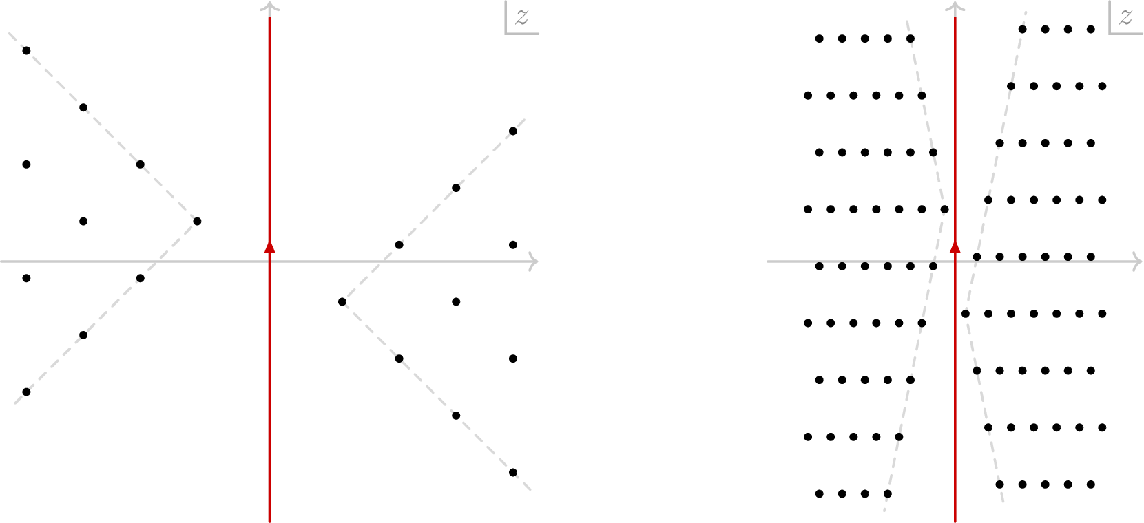
Let us describe the main steps of the reduction ?? . The integrand \(\mathcal{I}(z)\) 24 has poles at the points \[\begin{align} \begin{aligned} z_{\mathrm{poles}} & = \pm \biggl( m_1 \omega_1 + m_2 \omega_2 + \frac{\omega_1 + \omega_2}{2} - g \biggr) \\[6pt] & = \pm \bigl( \mathrm{i}(m_1 - m_2) + (m_1 + m_2 + 1) \delta - \mathrm{i}\sqrt{1 + \delta^2}(m + u \delta) \bigr), \end{aligned} \end{align}\] where \(m_1, m_2 \in \mathbb{Z}_{\geq 0}\). In the limit \(\delta \to 0^+\) these poles pinch integration contour \(\mathrm{i}\mathbb{R}\) at the points \(\mathrm{i}\mathbb{Z}\), as illustrated in Figure 3.

The first step is to convert the integral over \(z\) into the sum of integrals around pinched points \[\begin{align} \int_{\mathrm{i}\mathbb{R}} \mathcal{I}(z) \, \frac{dz}{\mathrm{i}\sqrt{\omega_1 \omega_2}} = \sum_{N \in \mathbb{Z}} \int_{- \frac{1}{2}}^{\frac{1}{2}} \mathcal{I}(\mathrm{i}\sqrt{\omega_1 \omega_2} \, [N + \beta]) \, d\beta. \end{align}\] Notice that the argument of \(\mathcal{I}\)-function on the right is the same, as in the limiting formula 28 .

Second, we cut off the sum at \(|N| = M/\delta\) \[\begin{align} \sum_{N \in \mathbb{Z}} \int_{- \frac{1}{2}}^{\frac{1}{2}} \mathcal{I}(\mathrm{i}\sqrt{\omega_1 \omega_2} \, [N + \beta]) \, d\beta = \lim_{M \to \infty} \sum_{|N| \leq M/\delta} \int_{- \frac{1}{2}}^{\frac{1}{2}} \mathcal{I}(\mathrm{i}\sqrt{\omega_1 \omega_2} \, [N + \beta]) \, d\beta \end{align}\] assuming \(M \in \mathbb{Z}_{>0}\). Note that the wedge slopes in Figure 3 are equal to \(1/\delta\), so that the distance from the point \(z = \mathrm{i}\sqrt{\omega_1 \omega_2} M/ \delta\) to the poles is of order one, as opposed to (say) \(z = 0\), for which the distance is of order \(\delta\).

Since the points with \(|N| \geq M/\delta\) experience no pinching, the tails of the above series (i.e. the sum over \(|N| \geq M/\delta\)) are expected to be bounded uniformly in \(\delta\). In Section 3.3 we prove that this is indeed the case and, as a result, we can interchange two limits \[\begin{gather} \label{change95lim} \lim_{\delta \to 0^+} \delta \lim_{M \to \infty} \sum_{|N| \leq M/\delta} \int_{- \frac{1}{2}}^{\frac{1}{2}} \mathcal{I}(\mathrm{i}\sqrt{\omega_1 \omega_2} \, [N + \beta]) \, d\beta \\[-6pt] = \lim_{M \to \infty} \, \lim_{\delta \to 0^+} \delta \sum_{|N| \leq M/\delta} \int_{- \frac{1}{2}}^{\frac{1}{2}} \mathcal{I}(\mathrm{i}\sqrt{\omega_1 \omega_2} \, [N + \beta]) \, d\beta. \end{gather}\tag{29}\] Mind that from the left we multiply the integral by \(\delta\) before taking the limit \(\delta \to 0^+\), as in the claimed formula ?? .

The final step is to calculate the limit \[\begin{align} \lim_{\delta \to 0^+} \delta \sum_{|N| \leq M/\delta} \int_{- \frac{1}{2}}^{\frac{1}{2}} \mathcal{I}(\mathrm{i}\sqrt{\omega_1 \omega_2} \, [N + \beta]) \, d\beta = \int_{-M}^M d\alpha \int_{-\frac{1}{2}}^{\frac{1}{2}} \mathcal{J}(\alpha, \beta) \, d\beta, \end{align}\] which is done in Section 3.4. The idea is that each term in the truncated sum suits the limiting formula 28 . In other words, for fixed \(N, \beta\) and small \(\delta\) the integrand \(\mathcal{I}(\mathrm{i}\sqrt{\omega_1 \omega_2} \, [N + \beta])\) is close to \(\mathcal{J}(N\delta, \beta)\), so it is reasonable to expect that \[\begin{align} \label{IJ-sums} \lim_{\delta \to 0^+} \delta \sum_{|N| \leq M/\delta} \int_{- \frac{1}{2}}^{\frac{1}{2}} \mathcal{I}(\mathrm{i}\sqrt{\omega_1 \omega_2} \, [N + \beta]) \, d\beta = \lim_{\delta \to 0^+} \delta \sum_{\substack{ |N| \leq M/\delta \\[2pt] N \neq 0}} \int_{- \frac{1}{2}}^{\frac{1}{2}} \mathcal{J}(N\delta, \beta) \, d\beta. \end{align}\tag{30}\] Note that we cannot add the term \(N = 0\) on the right, since \(\mathcal{J}(0, \beta)\) is not integrable for generic parameters. However, we show that the corresponding term on the left vanishes \[\begin{align} \label{I0-lim} \lim_{\delta \to 0^+} \delta \int_{- \frac{1}{2}}^{\frac{1}{2}} \mathcal{I}(\mathrm{i}\sqrt{\omega_1 \omega_2} \, \beta) \, d\beta = 0. \end{align}\tag{31}\] The above formulas require uniform bounds on ratios of the hyperbolic gamma functions, which we derive in Appendices 7 and 8.

At last, the sum on the right-hand side of 30 is a Riemann sum of mesh \(\delta\), so that \[\begin{align} \lim_{\delta \to 0^+} \delta \sum_{\substack{ |N| \leq M/\delta \\[2pt] N \neq 0}} \int_{- \frac{1}{2}}^{\frac{1}{2}} \mathcal{J}(N\delta, \beta) \, d\beta = \int_{-M}^M d\alpha \int_{-\frac{1}{2}}^{\frac{1}{2}} \mathcal{J}(\alpha, \beta) \, d\beta. \end{align}\] Although for some values of \(\relax u\) the integral over \(\alpha\) is improper, the above approximation still holds in this case, see Appendix 9.1. Taking \(M \to \infty\) we finish the reduction ?? .

3.3 Interchanging limits↩︎

In this section we prove that the interchange of two limits 29 is legitimate. Notice that the separate limit \(M\to\infty\) exists for any fixed \(\delta > 0\) due to the convergence of the initial hyperbolic integral. Besides, in Section 3.4 we show that the separate limit \(\delta \to 0^+\) also exists for any fixed \(M > 0\) (by calculating it explicitly). Hence, to interchange two limits it is sufficient to show that the limit \(M \to \infty\) is uniform for small enough \(\delta \leq \delta_{\mathrm{max}}\). Standardly, this is done by estimating the tails \[\begin{align} \label{Tail} \Biggl| \, \delta \sum_{| N| \geq M/\delta} \, \int_{- \frac{1}{2}}^{\frac{1}{2} } \mathcal{I}\bigl(\mathrm{i}\sqrt{\omega_1 \omega_2} \, [N + \beta] \bigr) \, d\beta \, \Biggr| \leq C_M \end{align}\tag{32}\] by a sequence of constants \(C_M\) independent of \(\delta\) and such that \[\begin{align} \lim_{M \to \infty} C_M = 0. \end{align}\] The main ingredient of the proof is Corollary 2 derived in Appendix 8.

Inserting parametrizations ?? , ?? into definition 24 and using reflection formula we rewrite the integrand as \[\begin{align} \label{Id-param} \mathcal{I}(\mathrm{i}\sqrt{\omega_1 \omega_2}[N + \beta]) = e^{-2\pi \mathrm{i}(N \delta v + \beta k + \beta v \delta )} \, \frac{\gamma^{(2)}\bigl(\mathrm{i}\sqrt{\omega_1 \omega_2} [N + \beta - m - (u + \mathrm{i}) \delta + \varepsilon(\delta) \delta^2 ]\bigr)}{ \gamma^{(2)}\bigl(\mathrm{i}\sqrt{\omega_1 \omega_2} [N + \beta + m + (u - \mathrm{i}) \delta + \varepsilon(\delta)\delta^2] \bigr) } , \end{align}\tag{33}\] where \[\begin{align} \varepsilon(\delta) = \frac{\mathrm{i}}{\delta} \biggl(1 - \frac{1}{\sqrt{1 + \delta^2}} \biggr)= O(\delta). \end{align}\] By Corollary 2 (with \(\nu = 1\)), the integrand satisfies the bound \[\begin{align} \label{C} \bigl| \mathcal{I}(\mathrm{i}\sqrt{\omega_1 \omega_2}[N + \beta]) \bigr| \leq C \bigl| 2\mathop{\mathrm{sh}}\pi (N \delta + \mathrm{i}\beta) \bigr|^{2\relax u} \end{align}\tag{34}\] uniformly for all \(|N| \geq 1/\delta\), \(0 < \delta \leq \delta_{\mathrm{max}}\) and \(|\beta| \leq 1\) with some constants \(C, \delta_{\mathrm{max}}\).

For large enough \(|N|\delta \geq M\) \[\begin{align} | 2\mathop{\mathrm{sh}}\pi (N \delta + \mathrm{i}\beta) | \geq 2\mathop{\mathrm{sh}}(\pi |N| \delta) \geq \frac{1}{2} e^{\pi |N| \delta}. \end{align}\] Furthermore, by assumption ?? , \(\relax u \in (-1, 0)\). Combining the above estimates we arrive at \[\begin{gather} \Biggl| \, \delta \sum_{| N| \geq M/\delta} \, \int_{- \frac{1}{2}}^{\frac{1}{2} } \mathcal{I}\bigl(\mathrm{i}\sqrt{\omega_1 \omega_2} \, [N + \beta] \bigr) \, d\beta \, \Biggr| \leq C' \delta \sum_{| N| \geq M/\delta} e^{-2 \pi |N| \delta |\relax u|} \\ = 2C' \delta \, \frac{e^{-2 \pi M |\relax u|}}{1 - e^{-2\pi \delta |\relax u|}} \leq C'' \, e^{-2 \pi M |\relax u|}, \end{gather}\] where on the last step we use the fact that \(\delta / (1 - e^{-2\pi \delta |\relax u|})\) is continuous for \(\delta \in [0, \delta_{\mathrm{max}}]\). Thus, the tails tend to zero uniformly in \(\delta\).

3.4 Calculating the \(\delta\)-limit↩︎

In this section we calculate the limit \[\begin{align} \label{IJ-calc-lim} \lim_{\delta \to 0^+} \delta \sum_{|N| \leq M/\delta} \int_{- \frac{1}{2}}^{\frac{1}{2}} \mathcal{I}(\mathrm{i}\sqrt{\omega_1 \omega_2} \, [N + \beta]) \, d\beta = \int_{-M}^M d\alpha \int_{-\frac{1}{2}}^{\frac{1}{2}} \mathcal{J}(\alpha, \beta) \, d\beta. \end{align}\tag{35}\] The main ingredients for this are the bounds derived in Proposition 1 and Corollary 3, as well as Lemma 5, which are proven in Appendix 8. Let us proceed with the following steps.

Step 1. Taking \(N_0 = |m| + 3\) let us prove that \[\begin{align} \label{sum-IJ} \lim_{\delta \to 0^+} \delta \sum_{N_0 + 1 \leq |N| \leq M/\delta} \int_{- \frac{1}{2}}^{\frac{1}{2}} \Bigl [ \mathcal{I}(\mathrm{i}\sqrt{\omega_1 \omega_2} \, [N + \beta]) - \mathcal{J}(N \delta, \beta) \Bigr] \, d\beta = 0. \end{align}\tag{36}\] If we factorise the expression 33 \[\begin{gather} \mathcal{I}(\mathrm{i}\sqrt{\omega_1 \omega_2}[N + \beta]) = e^{-2\pi \mathrm{i}(N \delta v + \beta k + \beta v \delta )} \, \frac{\gamma^{(2)}\bigl(\mathrm{i}\sqrt{\omega_1 \omega_2} [N + \beta - m - (u + \mathrm{i}) \delta + \varepsilon(\delta) \delta^2 ]\bigr)}{ \gamma^{(2)}\bigl(\mathrm{i}\sqrt{\omega_1 \omega_2} [N + \beta ] \bigr) } \\[8pt] \times \frac{\gamma^{(2)}\bigl(\mathrm{i}\sqrt{\omega_1 \omega_2} [N + \beta ]\bigr)}{ \gamma^{(2)}\bigl(\mathrm{i}\sqrt{\omega_1 \omega_2} [N + \beta + m + (u - \mathrm{i}) \delta + \varepsilon(\delta)\delta^2] \bigr) } , \end{gather}\] then for each ratio of gamma functions we can apply Proposition 1(ii) (here we use the condition \(|N| \geq N_0 + 1\)). If in addition we invoke Lemma 5, then for the function in square brackets we obtain the bound \[\begin{align} \bigl| \mathcal{I}(\mathrm{i}\sqrt{\omega_1 \omega_2} \, [N + \beta]) - \mathcal{J}(N \delta, \beta) \bigr| \leq \frac{C_1 \delta}{1 - e^{-C_2 |N| \delta}} \, \bigl| \mathcal{J}(N \delta, \beta) \bigr| \end{align}\] with some constants \(C_1, C_2 > 0\) uniform in \(N ,\delta, \beta\) inside considered intervals.

Furthermore, by definition 27 , for \(|\beta| \leq 1/2\) and \(N \ne 0\) we have \[\begin{gather} \label{Jd-abs} \bigl| \mathcal{J}(N\delta, \beta) \bigr| = \bigl| 2\mathop{\mathrm{sh}}\pi (N \delta + \mathrm{i}\beta) \bigr|^{2\relax u} = \bigl( 4\mathop{\mathrm{sh}}^2 (\pi N \delta) + 4 \sin^2(\pi \beta) \bigr)^{\relax u} \\[6pt] \leq C \, (\delta^2 + \beta^2)^{\relax u}, \end{gather}\tag{37}\] since \(\relax u \in (-1, 0)\). Using this and the fact that \(s/(1 - e^{-C_2 s})\) is bounded for \(s \in [0, M]\), we arrive at a simpler bound \[\begin{align} \bigl| \mathcal{I}(\mathrm{i}\sqrt{\omega_1 \omega_2} \, [N + \beta]) - \mathcal{J}(N \delta, \beta) \bigr| \leq \frac{C}{|N|} \, (\delta^2 + \beta^2)^{\relax u}. \end{align}\] Consequently, the whole sum is estimated as \[\begin{gather} \Biggl| \, \delta \sum_{N_0 + 1 \leq |N| \leq M/\delta} \int_{- \frac{1}{2}}^{\frac{1}{2}} \Bigl [ \mathcal{I}(\mathrm{i}\sqrt{\omega_1 \omega_2} \, [N + \beta]) - \mathcal{J}(N \delta, \beta) \Bigr] \, d\beta \, \Biggr| \\ \leq C \sum_{N_0 + 1 \leq |N| \leq M/\delta} \frac{1}{|N|} \; \; \delta \int_{- \frac{1}{2}}^{\frac{1}{2}} (\delta^2 + \beta^2)^{\relax u} \, d\beta . \end{gather}\] The sum over \(N\) is bounded by the harmonic numbers \[\begin{align} \sum_{N_0 + 1 \leq |N| \leq M/\delta} \frac{1}{|N|} \leq 2\sum_{N = 2}^{M/\delta} \frac{1}{N} \leq 2\ln \frac{M}{\delta}. \end{align}\] Besides, it is easy to show that the integral over \(\beta\) satisfies the bound \[\begin{align} \label{dbeta-int} \delta \int_{- \frac{1}{2}}^{\frac{1}{2}} (\delta^2 + \beta^2)^{\relax u} \, d\beta \leq C_1 \delta^{2(1 + \relax u)} + C_2 \delta \ln \frac{1}{\delta}, \end{align}\tag{38}\] see Lemma 6. The latter estimates imply the claim 36 .

Step 2. As one can see, formula 36 excludes the terms \(|N| \leq N_0\). Let us show that for these terms we have \[\begin{align} \lim_{\delta \to 0^+} \delta \int_{- \frac{1}{2}}^{\frac{1}{2}} \mathcal{I}(\mathrm{i}\sqrt{\omega_1 \omega_2} \, [N + \beta]) \, d\beta = 0. \end{align}\] By Corollary 3, for any \(N_0 \in \mathbb{Z}_{>0}\) we have the following bound for the integrand 33 \[\begin{align} \bigl| \mathcal{I}(\mathrm{i}\sqrt{\omega_1 \omega_2}[N + \beta]) \bigr| \leq A \, \bigl| 2\mathop{\mathrm{sh}}\pi (N \delta + 2k \mathop{\mathrm{sign}}(N) \delta + \mathrm{i}\beta) \bigr|^{2\relax u} \end{align}\] uniformly for all \(|N| \leq N_0\), \(0 < \delta \leq \delta_{\mathrm{max}}\) and \(|\beta| \leq 1\) with some constants \(A, \delta_{\mathrm{max}}>0\) and \(k \in \mathbb{Z}_{>0}\) (here \(\mathop{\mathrm{sign}}(0) = 1\)). Moreover, since in the above integral \(|\beta| \leq 1/2\) and \(\relax u \in (-1, 0)\), we have \[\begin{align} \label{sh-ineq} \bigl| \mathop{\mathrm{sh}}\pi (N \delta + 2k \mathop{\mathrm{sign}}(N) \delta + \mathrm{i}\beta) \bigr|^{2\relax u} \leq B \, (\delta^2 + \beta^2)^{\relax u} \end{align}\tag{39}\] with some constant \(B\). This leads to the bound for the integral \[\begin{align} \Biggl| \, \delta \int_{- \frac{1}{2}}^{\frac{1}{2}} \mathcal{I}(\mathrm{i}\sqrt{\omega_1 \omega_2} \, [N + \beta]) \, d\beta \, \Biggr| \leq C \delta \int_{- \frac{1}{2}}^{\frac{1}{2}} (\delta^2 + \beta^2)^{\relax u} \, d\beta. \end{align}\] Due to the inequality 38 the right-hand side tends to zero as \(\delta \to 0^+\).

Step 3. Similarly, for all \(|N| \leq N_0\), \(N \ne 0\), we have \[\begin{align} \lim_{\delta \to 0^+} \delta \int_{- \frac{1}{2}}^{\frac{1}{2}} \mathcal{J}(N\delta, \beta) \, d\beta = 0. \end{align}\] To show this one should use the bound 37 . The rest of the arguments are the same, as in the previous step.

Step 4. Combining the results of all previous steps we arrive at the relation \[\begin{align} \lim_{\delta \to 0^+} \delta \sum_{|N| \leq M/\delta } \int_{- \frac{1}{2}}^{\frac{1}{2}} \mathcal{I}(\mathrm{i}\sqrt{\omega_1 \omega_2} \, [N + \beta]) \, d\beta = \lim_{\delta \to 0^+} \delta \sum_{\substack{ |N| \leq M/\delta \\[2pt] N \neq 0}} \int_{- \frac{1}{2}}^{\frac{1}{2}} \mathcal{J}(N\delta, \beta) \, d\beta. \end{align}\] The right-hand side represents two Riemann sums (for \(N > 0\) and \(N < 0\)) approximating two integrals \[\begin{align} \label{Gd-int} \int_{-M}^0 \mathcal{G}(\alpha) \, d\alpha + \int_{0}^M \mathcal{G}(\alpha) \, d\alpha = \int_{-M}^M \mathcal{G}(\alpha) \, d\alpha, \qquad\quad \mathcal{G}(\alpha) = \int_{- \frac{1}{2}}^{\frac{1}{2}} \mathcal{J}(\alpha, \beta) \, d\beta. \end{align}\tag{40}\] To complete the calculation 35 we only need the statement \[\begin{align} \label{G-approx} \lim_{\delta \to 0^+} \delta \sum_{\substack{ |N| \leq M/\delta \\[2pt] N \neq 0}} \mathcal{G}(N \delta) = \int_{-M}^M \mathcal{G}(\alpha) \, d\alpha. \end{align}\tag{41}\] For proper Riemann integrals this is a general fact, however, such approximation may fail for improper ones depending on the function \(\mathcal{G}(\alpha)\). In our case \[\begin{align} |\mathcal{G}(\alpha)| \leq \int_{- \frac{1}{2}}^{\frac{1}{2}} \bigl| 2\mathop{\mathrm{sh}}\pi (\alpha + \mathrm{i}\beta) \bigr|^{2\relax u} \, d\beta \leq \bigl| 2\mathop{\mathrm{sh}}(\pi \alpha) \bigr|^{2\relax u}. \end{align}\] Hence, the integral over \(\beta\) is absolutely convergent for all \(\alpha \in \mathbb{R}\) only if \(\relax u \in (-1/2, 0)\).

So, depending on \(\relax u\), we have either a proper or improper Riemann integral over \(\alpha\). To conclude the proof, we check in Appendix 9.1 that the approximation 41 holds in the improper case as well.

4 From hyperbolic to complex rational conical function↩︎

The procedure described above can be also applied to the integrals that cannot be evaluated explicitly. One of such examples is given by the hyperbolic conical function, which we consider in this section.

4.1 Conical functions↩︎

The classical conical function (up to some inessential factors) represents a special case of the Gauss hypergeometric function \({}_2 F_1(a, b, c; z)\) with some restriction³ on the parameters \(a, b, c\), see [14].

In [11] Ruijsenaars introduced hyperbolic variant of the conical function and derived several integral representations for it. In particular, the representation [11] in our notation reads (use 8 and 10 ) \[\begin{gather} \mathcal{R}(\omega_1, \omega_2, 2g; \mathrm{i}x, \mathrm{i}\lambda) = \frac{\gamma^{(2)}(4g)}{\gamma^{(2)}(2g \pm \lambda)} \int_{\mathrm{i}\mathbb{R}} e^{ \frac{2\pi \mathrm{i}}{\omega_1 \omega_2} \lambda z } \, \gamma^{(2)} \biggl( z \pm \frac{ x}{2} + \frac{\omega_1 + \omega_2}{2} - g\biggr) \\ \times \gamma^{(2)} \biggl( - z \pm \frac{ x}{2} + \frac{\omega_1 + \omega_2}{2} - g \biggr) \, \frac{dz}{\mathrm{i}\sqrt{\omega_1 \omega_2}}. \end{gather}\] Due to the asymptotics 9 , this integral is well defined and the integration contour separates series of poles of gamma functions for \(x, \lambda \in \mathrm{i}\mathbb{R}\) and \(0 < \relax g < \relax(\omega_1 + \omega_2)/2\). In what follows it will be more convenient for us to work with the function \[\begin{gather} \label{Psi} \Psi_\lambda(x; g) \equiv \Psi_\lambda(x; g , \omega_1, \omega_2) = \int_{\mathrm{i}\mathbb{R}} e^{ \frac{2\pi \mathrm{i}}{\omega_1 \omega_2} \lambda z } \, \gamma^{(2)} \biggl( \pm z + \frac{\omega_1 + \omega_2}{2} - g \biggr) \\ \times \gamma^{(2)} \biggl( \pm (z - x) + \frac{\omega_1 + \omega_2}{2} - g \biggr) \, \frac{dz}{\mathrm{i}\sqrt{\omega_1 \omega_2}}, \end{gather}\tag{42}\] which transforms into the previous one after the shift of integration variable \(z \to z + x/2\) modulo the integral prefactors.

The above function reduces to the Gauss hypergeometric function in the limit \(\omega_1 \to 0^+\). Namely, assuming \(\omega_1, \omega_2, g> 0\) and using the limiting formula 14 we have \[\begin{align} \label{con-cl-lim} \lim_{\omega_1 \to 0^+} \sqrt{ \frac{\omega_1}{\omega_2} } \, \Psi_{v \omega_1}(x; u \omega_1) = \int_{\mathrm{i}\mathbb{R}} e^{\frac{2\pi \mathrm{i}}{\omega_2} v z} \, \biggl( 2 \cos \frac{\pi z}{\omega_2} \biggr)^{-2u} \, \biggl( 2 \cos \frac{\pi (z - x)}{\omega_2} \biggr)^{-2u} \, \frac{dz}{\mathrm{i}\omega_2} , \end{align}\tag{43}\] where the interchange of the limit and integration can be justified using the uniform bound 15 . The last integral turns into the Euler representation of hypergeometric function \[\begin{align} {}_2 F_1(a, b, c; w) = \frac{\Gamma(c)}{\Gamma(b)\Gamma(c - b)} \int_0^1 t^{b - 1} (1 - t)^{c - b - 1} (1 - wt)^{-a} \, dt \end{align}\] after the change of variable \(t = 1/(1 + e^{2\pi \mathrm{i}z/\omega_2})\) (in this way we obtain the special case of hypergeometric function with restriction \(c = 2a\)).

Notice that the function 42 is similar to the hyperbolic beta integral 11 . The difference is that the integrand \[\begin{align} \label{Idc} \mathcal{I}_c(z) = e^{ \frac{2\pi \mathrm{i}}{\omega_1 \omega_2} \lambda z } \, \gamma^{(2)} \biggl( \pm z + \frac{\omega_1 + \omega_2}{2} - g \biggr) \, \gamma^{(2)} \biggl( \pm (z - x) + \frac{\omega_1 + \omega_2}{2} - g \biggr) \end{align}\tag{44}\] contains two more gamma functions and the additional parameter \(x\), which appears in the position similar to the integration variable \(z\). This suggests that the hyperbolic conical function also has a complex rational reduction. To describe it we parametrise, as before, \(\omega_1 = \bar{\omega}_2 = \mathrm{i}+ \delta\) and take \[\begin{align} \label{glx-param} \begin{aligned} & g = \mathrm{i}\sqrt{\omega_1 \omega_2}(m + u \delta), &&m \in \mathbb{Z}, &&\relax u \in (-1, 0), \\[6pt] & \lambda = \mathrm{i}\sqrt{\omega_1 \omega_2}(k + v \delta), &&k\in \mathbb{Z}, &&v \in \mathbb{R}, \\[2pt] & x = \mathrm{i}\sqrt{\omega_1 \omega_2} (K(\delta) + \sigma), &&K(\delta) \in \mathbb{Z}, &&|\sigma| \leq \frac{1}{2}, \end{aligned} \end{align}\tag{45}\] such that \(K(\delta) \delta \to \rho \in \mathbb{R}\) as \(\delta \to 0^+\). Then due to 19 the integrand has the limit \[\begin{align} \mathcal{I}_c(\mathrm{i}\sqrt{\omega_1 \omega_2}[N + \beta]) \underset{\substack{\delta \to 0^+\\[2pt] N\delta \to \alpha \; \,}}{=} \mathcal{J}_c(\alpha, \beta), \end{align}\] where \[\begin{gather} \label{Jdc} \mathcal{J}_c(\alpha, \beta) = e^{-2\pi \mathrm{i}(\alpha v + \beta k)} \, \bigl( 2\mathop{\mathrm{sh}}\pi (\alpha + \mathrm{i}\beta) \; 2\mathop{\mathrm{sh}}\pi (\alpha - \rho + \mathrm{i}\beta - \mathrm{i}\sigma) \bigr)^{-m - \mathrm{i}u} \\[6pt] \times \bigl(2\mathop{\mathrm{sh}}\pi (\alpha - \mathrm{i}\beta) \; 2\mathop{\mathrm{sh}}\pi (\alpha - \rho - \mathrm{i}\beta + \mathrm{i}\sigma) \bigr)^{m - \mathrm{i}u} . \end{gather}\tag{46}\] Hence, analogously to the case of beta integral ?? , it is reasonable to expect the following statement.

The proof is given in Sections 4.2–4.4, but before that let us make a few remarks. First, the resulting integral on the right \[\begin{gather} \label{Phi} \Phi_{v, k}(\rho, \sigma; u, m) = \int_{\mathbb{R}} d\alpha \int_{-\frac{1}{2}}^{\frac{1}{2}} e^{-2\pi \mathrm{i}(\alpha v + \beta k)} \, \bigl( 2\mathop{\mathrm{sh}}\pi (\alpha + \mathrm{i}\beta) \; 2\mathop{\mathrm{sh}}\pi (\alpha - \rho + \mathrm{i}\beta - \mathrm{i}\sigma) \bigr)^{-m - \mathrm{i}u} \\ \times \bigl(2\mathop{\mathrm{sh}}\pi (\alpha - \mathrm{i}\beta) \; 2\mathop{\mathrm{sh}}\pi (\alpha - \rho - \mathrm{i}\beta + \mathrm{i}\sigma) \bigr)^{m - \mathrm{i}u} \, d\beta \end{gather}\tag{47}\] is essentially the conical function of complex rational type. After the change of variable \(z = 1/(1 - e^{2\pi(\alpha + \mathrm{i}\beta)})\) it transforms into the special case of the hypergeometric function associated with the complex field (modulo some integral prefactors) \[\begin{align} {}_2F_1^{\mathbb{C}}(a|a', b|b', c|c'; w,\bar{w}) = \frac{\boldsymbol{\Gamma}(c|c')}{\pi \boldsymbol{\Gamma}(b|b') \boldsymbol{\Gamma}(c - b| c' - b')} \int_{\mathbb{C}} [z]^{b - 1} [1 - z]^{c - b - 1} [1 - w z]^{-a} \, d^2z, \end{align}\] as introduced in [5]. Here we assume that \(a - a', b - b', c - c' \in \mathbb{Z}\), and the integral converges in some domain of parameters, see [15].

Secondly, we remark that formula ?? in fact follows from the results of our previous paper [16]. The hyperbolic conical function can be interpreted as the eigenfunction of hyperbolic Ruijsenaars system Hamiltonians in the case of two particles (see [17]), and in [16] we have considered complex rational limit of this system. Correspondingly, the claim ?? follows from the combination of formulas [16] and 17 .

However, this reasoning is non-direct: to establish the limit ?? in [16] we pass to the “dual” Mellin–Barnes integral representations of the corresponding functions. So, it is desirable to give a more straightforward proof, which is done in the next sections.

Finally, let us comment about the assumptions on the parameters. The conditions on \(\delta, v, u\) have the same reasons, as in the situation of beta integral. The case of arbitrary \(K(\delta)\), such that \(K(\delta) \delta \to \rho\), requires only inessential modifications, which complicate the exposition, so for brevity we fix \(K(\delta)\). Besides, if \(\rho = 0\), then nothing changes in the calculation of the limit in comparison with the beta integral, however, if additionally \(\sigma = 0\) one must assume a stronger condition \(\relax u \in (-1/2, 0)\) for the limiting integral to be absolutely convergent.

4.2 Outline↩︎

Let us describe the main steps of reduction ?? . In what follows we assume \(\rho > 0\) without loss of generality due to the symmetry \(\Psi_\lambda(x; g) = \Psi_{-\lambda}(-x; g)\).

As before, the first step is to transform the integral 42 into the series \[\begin{align} \int_{\mathrm{i}\mathbb{R}} \mathcal{I}_c(z) \, \frac{dz}{\mathrm{i}\sqrt{\omega_1 \omega_2}} = \sum_{N \in \mathbb{Z}} \int_{- \frac{1}{2}}^{\frac{1}{2}} \mathcal{I}_c(\mathrm{i}\sqrt{\omega_1 \omega_2} \, [N + \beta]) \, d\beta. \end{align}\] In the limit \(\delta \to 0^+\) poles of the integrand 44 pinch the integration contour at the points \(\mathrm{i}\mathbb{Z}\) and \(\mathrm{i}(\mathbb{Z} + \sigma)\), however, there is no pinching for the points sufficiently far away (e.g., \(|z| \geq \sqrt{\omega_1 \omega_2} (\rho + 1)/\delta\)). Hence, we cut off the series at \(|N| = M/\delta\) (\(M \in \mathbb{Z}_{>0}\)) and prove that one can interchange two limits \[\begin{align} \label{con-lim-switch} \Bigl(\lim_{\delta \to 0^+} \, \lim_{M \to \infty}- \lim_{M \to \infty} \, \lim_{\delta \to 0^+} \Bigr) \; \delta \sum_{|N| \leq M/\delta} \int_{- \frac{1}{2}}^{\frac{1}{2}} \mathcal{I}_c(\mathrm{i}\sqrt{\omega_1 \omega_2} \, [N + \beta]) \, d\beta =0, \end{align}\tag{48}\] see Section 4.3.

Next, in Section 4.4 we calculate the \(\delta\)-limit \[\begin{align} \label{limit95con} \lim_{\delta \to 0^+} \delta \sum_{|N| \leq M/\delta} \int_{- \frac{1}{2}}^{\frac{1}{2}} \mathcal{I}_c(\mathrm{i}\sqrt{\omega_1 \omega_2} \, [N + \beta]) \, d\beta = \int_{-M}^M d\alpha \int_{-\frac{1}{2}}^{\frac{1}{2}} \mathcal{J}_c(\alpha, \beta) \, d\beta \end{align}\tag{49}\] for large enough \(M\). For this we first show that \[\begin{gather} \lim_{\delta \to 0^+} \delta \sum_{|N| \leq M/\delta} \int_{- \frac{1}{2}}^{\frac{1}{2}} \mathcal{I}_c(\mathrm{i}\sqrt{\omega_1 \omega_2} \, [N + \beta]) \, d\beta \\ = \lim_{\delta \to 0^+} \delta \Biggl( \sum_{N = -M/\delta}^{-1} + \sum_{N = 1}^{\lfloor \rho/\delta \rfloor - 1} + \sum_{N = \lfloor \rho/\delta \rfloor + 2}^{M/\delta} \Biggr) \int_{- \frac{1}{2}}^{\frac{1}{2}} \mathcal{J}_c(N\delta, \beta) \, d\beta. \end{gather}\] Notice the difference with the beta integral case 30 . If \(\relax u \leq -1/2\) the function \(\mathcal{J}_c(\alpha, \beta)\) is not integrable in \(\beta\) for \(\alpha = 0\) and \(\alpha = \rho\), see 46 . To avoid these singular points we exclude the terms \(N = 0\), \(N = \lfloor \rho/\delta\rfloor\) and \(N = \lfloor \rho/\delta\rfloor + 1\) on the right-hand side (both \(\lfloor \rho/\delta\rfloor\) and \(\lfloor \rho/\delta\rfloor + 1\) can be arbitrarily close to \(\rho/\delta\) as \(\delta \to 0^+\)).

The last step is to prove that the right-hand side approximates the Riemann integral in \(\alpha\) \[\begin{align} \lim_{\delta \to 0^+} \delta \Biggl( \sum_{N = -M/\delta}^{-1} + \sum_{N = 1}^{\lfloor \rho/\delta \rfloor - 1} + \sum_{N = \lfloor \rho/\delta \rfloor + 2}^{M/\delta} \Biggr) \int_{- \frac{1}{2}}^{\frac{1}{2}} \mathcal{J}_c(N\delta, \beta) \, d\beta = \int_{-M}^M d\alpha \int_{-\frac{1}{2}}^{\frac{1}{2}} \mathcal{J}_c(\alpha, \beta) \, d\beta. \end{align}\] This statement is intuitively clear, while the detailed analysis is given in Appendix 9.2. Taking \(M \to \infty\) we complete the reduction ?? .

4.3 Interchanging limits↩︎

In this part there is almost nothing new in comparison to the beta integral case. To interchange two limits 48 it is sufficient to estimate the tails \[\begin{align} \Biggl| \, \delta \sum_{| N| \geq M/\delta} \, \int_{- \frac{1}{2}}^{\frac{1}{2} } \mathcal{I}_c\bigl(\mathrm{i}\sqrt{\omega_1 \omega_2} \, [N + \beta] \bigr) \, d\beta \, \Biggr| \leq C_M \end{align}\] by constants \(C_M\) independent of \(\delta\) and vanishing as \(M \to \infty\).

With the parametrisation 45 the integrand 44 has the following form (after application of the reflection relation 8 ) \[\begin{gather} \mathcal{I}_c(\mathrm{i}\sqrt{\omega_1 \omega_2}[N + \beta]) = e^{-2\pi \mathrm{i}(N \delta v + \beta k + \beta v \delta )} \, \frac{\gamma^{(2)}\bigl(\mathrm{i}\sqrt{\omega_1 \omega_2} [N + \beta - m - (u + \mathrm{i}) \delta + \varepsilon(\delta) \delta^2 ]\bigr)}{ \gamma^{(2)}\bigl(\mathrm{i}\sqrt{\omega_1 \omega_2} [N + \beta + m + (u - \mathrm{i}) \delta + \varepsilon(\delta)\delta^2] \bigr) } \\[6pt] \times \frac{\gamma^{(2)}\bigl(\mathrm{i}\sqrt{\omega_1 \omega_2} [N - \lfloor \rho/\delta \rfloor + \beta - \sigma - m - (u + \mathrm{i}) \delta + \varepsilon(\delta) \delta^2 ]\bigr)}{ \gamma^{(2)}\bigl(\mathrm{i}\sqrt{\omega_1 \omega_2} [N - \lfloor \rho/\delta \rfloor + \beta - \sigma + m + (u - \mathrm{i}) \delta + \varepsilon(\delta)\delta^2] \bigr) } , \end{gather}\] where \(\varepsilon(\delta) = \mathrm{i}(1 - 1/\sqrt{1 + \delta^2} ) / \delta\). For \(|N| \geq M/\delta \geq (\rho + 1)/\delta\) we have \[\begin{align} \biggl| N - \biggl\lfloor \frac{\rho}{\delta} \biggr\rfloor \biggr| \geq \frac{M}{\delta} - \biggl\lfloor \frac{\rho}{\delta} \biggr\rfloor \geq \frac{1}{\delta}. \end{align}\] Hence, we can use Corollary 2 (with \(\nu = 1\)) to obtain the bound \[\begin{align} \bigl| \mathcal{I}_c(\mathrm{i}\sqrt{\omega_1 \omega_2}[N + \beta]) \bigr| \leq C \, \bigl| 2\mathop{\mathrm{sh}}\pi (N \delta + \mathrm{i}\beta) \; 2\mathop{\mathrm{sh}}\pi (N - \lfloor \rho/\delta \rfloor \delta + \mathrm{i}\beta - \mathrm{i}\sigma) \bigr|^{2\relax u} \end{align}\] uniform in \(N, \delta, \beta\) inside the considered intervals. Furthermore, for sufficiently large \(|N| \delta \geq M\) \[\begin{align} \bigl| 2\mathop{\mathrm{sh}}\pi (N \delta + \mathrm{i}\beta) \; 2\mathop{\mathrm{sh}}\pi (N - \lfloor \rho/\delta \rfloor \delta + \mathrm{i}\beta - \mathrm{i}\sigma) \bigr| \geq \frac{1}{2} e^{\pi (|N| + |N - \lfloor \rho/\delta \rfloor|)\delta} \geq \frac{1}{2} e^{2\pi |N| \delta - \pi \rho}. \end{align}\] Since \(\relax u \in (-1, 0)\) we therefore have \[\begin{align} \Biggl| \, \delta \sum_{| N| \geq M/\delta} \, \int_{- \frac{1}{2}}^{\frac{1}{2} } \mathcal{I}_c\bigl(\mathrm{i}\sqrt{\omega_1 \omega_2} \, [N + \beta] \bigr) \, d\beta \, \Biggr| \leq C\delta \sum_{|N| \geq M/\delta} e^{-4\pi |N| \delta | \relax u |} \leq C' e^{-4\pi | \relax u | M}, \end{align}\] which implies the claim.

4.4 Calculating the \(\delta\)-limit↩︎

In this section we calculate the limit 49 assuming sufficiently large \(M\). Overall, the calculation is quite similar to that for the beta integral. It does, however, require a slightly more intricate manipulation of the bounds from Appendix 8, so we provide the details.

As shown in Appendix 9.2, due to the singularities at \(\alpha = 0\) and \(\alpha = \rho\), in general case the right-hand side of 49 is approximated by three (Riemann-type) sums \[\begin{align} \label{J-int-riem} \lim_{\delta \to 0^+} \delta \Biggl( \sum_{N = -M/\delta}^{-1} + \sum_{N = 1}^{\lfloor \rho/\delta \rfloor - 1} + \sum_{N = \lfloor \rho/\delta \rfloor + 2}^{M/\delta} \Biggr) \int_{- \frac{1}{2}}^{\frac{1}{2}} \mathcal{J}_c(N\delta, \beta) \, d\beta = \int_{-M}^M d\alpha \int_{-\frac{1}{2}}^{\frac{1}{2}} \mathcal{J}_c(\alpha, \beta) \, d\beta. \end{align}\tag{50}\] It remains to analyse the difference between the left-hand sides of 49 and 50 .

Step 1. Take \(N_0 = |m| + 3\) and consider the terms away from \(N = 0\) and \(N = \lfloor \rho/\delta \rfloor\) by at least \(N_0 + 1\). For them we prove that \[\begin{gather} \label{IJ-sum-N0} \lim_{\delta \to 0^+} \delta \Biggl( \sum_{N = -M/\delta}^{-N_0 - 1} + \sum_{N = N_0 + 1}^{\lfloor \rho/\delta \rfloor - 1 - N_0} + \sum_{N = \lfloor \rho/\delta \rfloor + 1 + N_0}^{M/\delta} \Biggr) \\[6pt] \times \int_{- \frac{1}{2}}^{\frac{1}{2}} \bigl[ \mathcal{I}_c(\mathrm{i}\sqrt{\omega_1 \omega_2} \, [N + \beta]) - \mathcal{J}_c(N\delta, \beta) \bigr] \, d\beta = 0. \end{gather}\tag{51}\] Let us consider the last sum, the arguments for the remaining two are analogous.

First, we show that \[\begin{align} \label{Idc-Jdc-ratio} \Biggl| \frac{ \mathcal{I}_c(\mathrm{i}\sqrt{\omega_1 \omega_2} \, [N + \beta]) }{ \mathcal{J}_c(N\delta, \beta) } - 1 \Biggr| \leq \frac{C_1 \delta}{1 - e^{-C_2 (N \delta - \rho)}} \end{align}\tag{52}\] with some constants \(C_1, C_2 > 0\) uniform in \(N, \delta, \beta\) in the considered intervals. Let us write \(\mathcal{J}_c(\alpha, \beta) \equiv \mathcal{J}_c(\alpha, \beta; \rho)\) to emphasize the dependence on the parameter \(\rho\), see 46 . Factorise the expression in question \[\begin{align} \frac{ \mathcal{I}_c(\mathrm{i}\sqrt{\omega_1 \omega_2} \, [N + \beta]) }{ \mathcal{J}_c(N\delta, \beta; \rho) } = \frac{ \mathcal{I}_c(\mathrm{i}\sqrt{\omega_1 \omega_2} \, [N + \beta]) }{ \mathcal{J}_c(N\delta, \beta; \lfloor \rho/\delta \rfloor \delta) } \; \frac{\mathcal{J}_c(N\delta, \beta; \lfloor \rho/\delta \rfloor \delta) }{ \mathcal{J}_c(N\delta, \beta; \rho) }. \end{align}\] Since in the sum \(N - \lfloor \rho/\delta \rfloor \geq N_0 + 1\) and \(|\beta - \sigma| \leq 1\), we can use Proposition 1(ii) together with Lemma 5 for the first ratio \[\begin{align} \label{Idc-Jdc-ratio-2} \Biggl| \frac{ \mathcal{I}_c(\mathrm{i}\sqrt{\omega_1 \omega_2} \, [N + \beta]) }{ \mathcal{J}_c(N\delta, \beta; \lfloor \rho/\delta \rfloor \delta) } - 1 \Biggr| \leq \frac{C_1 \delta}{1 - e^{-C_2 (N - \lfloor \rho/\delta \rfloor)\delta}} \leq \frac{C_1 \delta}{1 - e^{-C_2 (N \delta - \rho)}}. \end{align}\tag{53}\] The second ratio explicitly reads \[\begin{align} \label{Jdc-ratio} \begin{aligned} \frac{\mathcal{J}_c(N\delta, \beta; \lfloor \rho/\delta \rfloor \delta) }{ \mathcal{J}_c(N\delta, \beta; \rho) } & = \biggl( \frac{2\mathop{\mathrm{sh}}\pi (N \delta - \rho + \mathrm{i}\beta - \mathrm{i}\sigma)}{2\mathop{\mathrm{sh}}\pi (N \delta - \lfloor\rho/\delta\rfloor \delta + \mathrm{i}\beta - \mathrm{i}\sigma)} \biggr)^{m + \mathrm{i}u} \\[6pt] & \times \biggl( \frac{2\mathop{\mathrm{sh}}\pi (N \delta - \rho - \mathrm{i}\beta + \mathrm{i}\sigma)}{2\mathop{\mathrm{sh}}\pi (N \delta - \lfloor\rho/\delta\rfloor \delta - \mathrm{i}\beta + \mathrm{i}\sigma)} \biggr)^{-m + \mathrm{i}u}. \end{aligned} \end{align}\tag{54}\] Rewrite the first ratio of sines \[\begin{align} \frac{2\mathop{\mathrm{sh}}\pi (N \delta - \rho + \mathrm{i}\beta - \mathrm{i}\sigma)}{2\mathop{\mathrm{sh}}\pi (N \delta - \lfloor\rho/\delta\rfloor \delta + \mathrm{i}\beta - \mathrm{i}\sigma)} = e^{\pi (\lfloor \rho/\delta \rfloor \delta - \rho)} \, \frac{ 1 - e^{-2\pi (N \delta - \rho + \mathrm{i}\beta - \mathrm{i}\sigma)} }{ 1 - e^{-2\pi (N \delta - \lfloor\rho/\delta\rfloor \delta + \mathrm{i}\beta - \mathrm{i}\sigma)} }, \end{align}\] and analogously for the second one. By Lemma 3 (with \(\mu = \rho/\delta - \lfloor\rho/\delta\rfloor\)), \[\begin{gather} \Bigl| \ln \bigl( 1 - e^{-2\pi (N \delta - \rho + \mathrm{i}\tau)} \bigr) - \ln \bigl( 1 - e^{-2\pi (N \delta - \lfloor\rho/\delta\rfloor \delta + \mathrm{i}\tau)} \bigr) \Bigr| \\[6pt] \leq \frac{2\pi(\rho/\delta - \lfloor\rho/\delta\rfloor) \delta}{1 - e^{-2\pi (N \delta- \rho)}} \leq \frac{2\pi \delta}{1 - e^{-2\pi (N \delta - \rho)}}. \end{gather}\] Using this inequality together with Lemmas 4, 5 we conclude that the second ratio given by 54 admits the same bound, as the first one, \[\begin{align} \label{Jdc-ratio-2} \Biggl| \frac{\mathcal{J}_c(N\delta, \beta; \lfloor \rho/\delta \rfloor \delta) }{ \mathcal{J}_c(N\delta, \beta; \rho) } - 1 \Biggr| \leq \frac{D_1 \delta}{1 - e^{-D_2 (N \delta - \rho)}} \end{align}\tag{55}\] with some \(D_1, D_2>0\). Thus, from the bounds 53 and 55 , using again Lemma 5, we obtain the estimate 52 .

As a result, we have the bound \[\begin{gather} \Biggl| \delta \sum_{N = \lfloor \rho/\delta \rfloor + 1 + N_0}^{M/\delta} \int_{- \frac{1}{2}}^{\frac{1}{2}} \bigl[ \mathcal{I}_c(\mathrm{i}\sqrt{\omega_1 \omega_2} \, [N + \beta]) - \mathcal{J}_c(N\delta, \beta) \bigr] \, d\beta \Biggr| \\ \leq \sum_{N = \lfloor \rho/\delta \rfloor + 1 + N_0}^{M/\delta} \frac{C_1 \delta}{1 - e^{-C_2 (N\delta - \rho)}} \; \delta \int_{- \frac{1}{2}}^{\frac{1}{2}} \bigl| \mathcal{J}_c(N\delta, \beta)\bigr| d\beta. \end{gather}\] The function \(\mathcal{J}_c(N\delta, \beta)\) is \(1\)-periodic in \(\beta\), so in the above integral we can change the integration domain to \([\sigma - 1/2, \sigma + 1/2]\). Furthermore, from the definition 46 we have \[\begin{align} \label{Jdc-abs} \bigl| \mathcal{J}_c(N\delta, \beta) \bigr| = \bigl| 2\mathop{\mathrm{sh}}\pi(N\delta + \mathrm{i}\beta) \; 2\mathop{\mathrm{sh}}\pi (N\delta - \rho + \mathrm{i}\beta - \mathrm{i}\sigma) \bigr|^{2 \relax u}. \end{align}\tag{56}\] The inequalities \[\begin{align} & \bigl| 2\mathop{\mathrm{sh}}\pi(N\delta + \mathrm{i}\beta) \bigr| \geq A, \qquad \bigl| 2\mathop{\mathrm{sh}}\pi (N\delta - \rho + \mathrm{i}\beta - \mathrm{i}\sigma) \bigr|^2 \geq B(\delta^2 + (\beta - \sigma)^2) \end{align}\] with some constants \(A, B\) hold for all \(N \geq \lfloor \rho/\delta \rfloor + 1 + N_0\) and \(\beta \in [\sigma - 1/2, \sigma + 1/2]\). Hence, the sum and integral can be separated \[\begin{gather} \Biggl| \delta \sum_{N = \lfloor \rho/\delta \rfloor + 1 + N_0}^{M/\delta} \int_{- \frac{1}{2}}^{\frac{1}{2}} \bigl[ \mathcal{I}_c(\mathrm{i}\sqrt{\omega_1 \omega_2} \, [N + \beta]) - \mathcal{J}_c(N\delta, \beta) \bigr] \, d\beta \Biggr| \\ \leq C \sum_{N = \lfloor \rho/\delta \rfloor + 1 + N_0}^{M/\delta} \frac{\delta}{1 - e^{-C_2 (N\delta - \rho)}} \; \delta \int_{- \frac{1}{2}}^{\frac{1}{2}} (\delta^2 + \beta^2)^{\relax u} d\beta. \end{gather}\] The sum is bounded by the harmonic numbers \[\begin{gather} \sum_{N = \lfloor \rho/\delta \rfloor + 1 + N_0}^{M/\delta} \frac{\delta}{1 - e^{-C_2 (N\delta - \rho)}} = \sum_{N = \lfloor \rho/\delta \rfloor + 1 + N_0}^{M/\delta} \frac{N\delta - \rho}{1 - e^{-C_2 (N\delta - \rho)}} \, \frac{1}{N - \rho/\delta} \\ \leq C \sum_{N = \lfloor \rho/\delta \rfloor + 1 + N_0}^{M/\delta} \frac{1}{N - \rho/\delta} \leq C \sum_{n = 2}^{M/\delta} \frac{1}{n} \leq C \ln \frac{M}{\delta}. \end{gather}\] Combining this with the bound on the \(\beta\)-integral given by Lemma 6 we come to the claim.

Step 2. Formula 51 excludes the terms \(|N| \leq N_0\) and \(|N - \lfloor \rho/\delta \rfloor | \leq N_0\). Let us prove that for them we have \[\begin{align} \lim_{\delta \to 0^+} \delta \int_{- \frac{1}{2}}^{\frac{1}{2}} \mathcal{I}_c(\mathrm{i}\sqrt{\omega_1 \omega_2} \, [N + \beta]) \, d\beta = 0. \end{align}\] Consider the case \(|N| \leq N_0\), arguments for the remaining values \(|N - \lfloor \rho/\delta \rfloor | \leq N_0\) are the same. In this case the integrand \[\begin{gather} \bigl| \mathcal{I}_c(\mathrm{i}\sqrt{\omega_1 \omega_2} \, [N + \beta]) \bigr| = \Biggl| \frac{\gamma^{(2)}\bigl(\mathrm{i}\sqrt{\omega_1 \omega_2} [N + \beta - m - (u + \mathrm{i}) \delta + O(\delta^2) ]\bigr)}{ \gamma^{(2)}\bigl(\mathrm{i}\sqrt{\omega_1 \omega_2} [N + \beta + m + (u - \mathrm{i}) \delta + O(\delta^2)] \bigr) } \\[6pt] \times \frac{\gamma^{(2)}\bigl(\mathrm{i}\sqrt{\omega_1 \omega_2} [N - \lfloor \rho/\delta \rfloor + \beta - \sigma - m - (u + \mathrm{i}) \delta + O(\delta^2) ]\bigr)}{ \gamma^{(2)}\bigl(\mathrm{i}\sqrt{\omega_1 \omega_2} [N - \lfloor \rho/\delta \rfloor + \beta - \sigma + m + (u - \mathrm{i}) \delta + O(\delta^2) ] \bigr) } \Biggr|, \end{gather}\] can be bounded using Corollaries 2 and 3 for the second and the first ratios correspondingly. Namely, from them we have \[\begin{gather} \bigl| \mathcal{I}_c(\mathrm{i}\sqrt{\omega_1 \omega_2} \, [N + \beta]) \bigr| \leq C \bigl| 2\mathop{\mathrm{sh}}\pi(N\delta + 2k \mathop{\mathrm{sign}}(N) \delta + \mathrm{i}\beta) \bigr|^{2\relax u} \\[6pt] \times \bigl| 2\mathop{\mathrm{sh}}\pi(N \delta - \lfloor \rho/\delta \rfloor \delta + \mathrm{i}\beta - \mathrm{i}\sigma ) \bigr|^{2\relax u} \end{gather}\] with some \(C\) and \(k \in \mathbb{Z}_{>0}\) for all \(N, \delta, \beta\) (here \(\mathop{\mathrm{sign}}(0) = 1\)). Under taken restrictions on the parameters and for a sufficiently small \(\delta\) the hyperbolic sines satisfy the bounds \[\begin{align} & \bigl| 2\mathop{\mathrm{sh}}\pi(N\delta + 2k \mathop{\mathrm{sign}}(N) \delta + \mathrm{i}\beta) \bigr|^2 \geq A (\delta^2 + \beta^2), \\[6pt] & \bigl| 2\mathop{\mathrm{sh}}\pi(N \delta - \lfloor \rho/\delta \rfloor \delta + \mathrm{i}\beta - \mathrm{i}\sigma ) \bigr| \geq \bigl| 2 \mathop{\mathrm{sh}}\pi (N - \lfloor \rho/\delta \rfloor) \delta \bigr| \geq B \end{align}\] with some constants \(A, B\). Therefore, \[\begin{align} \biggl| \delta \int_{- \frac{1}{2}}^{\frac{1}{2}} \mathcal{I}_c(\mathrm{i}\sqrt{\omega_1 \omega_2} \, [N + \beta]) \, d\beta \biggr| \leq C \delta \int_{- \frac{1}{2}}^{\frac{1}{2}} (\delta^2 + \beta^2)^{\relax u}. \end{align}\] The right-hand side tends to zero as \(\delta \to 0^+\) due to Lemma 6.

Step 3. Analogously, for \(|N| \leq N_0\) or \(|N - \lfloor \rho/\delta \rfloor | \leq N_0\) with \(N \ne 0, \lfloor \rho/\delta \rfloor, \lfloor \rho/\delta \rfloor + 1\) we have \[\begin{align} \lim_{\delta \to 0^+} \delta \int_{- \frac{1}{2}}^{\frac{1}{2}} \mathcal{J}_c(N\delta, \beta) \, d\beta = 0. \end{align}\] To prove it use 56 , the rest of arguments are the same, as at the previous step. Let us remark that we exclude \(N = 0, \lfloor \rho/\delta \rfloor, \lfloor \rho/\delta \rfloor + 1\) to have \(|N| \geq 1\) and \(|N - \rho/\delta| \geq 1\), that is to avoid singular points \(\alpha = 0, \rho\) of the function \(\mathcal{J}_c(\alpha, \beta)\).

Step 4. Combining the results of all the previous steps we arrive at the equality \[\begin{gather} \lim_{\delta \to 0^+} \delta \sum_{|N| \leq M/\delta} \int_{- \frac{1}{2}}^{\frac{1}{2}} \mathcal{I}_c(\mathrm{i}\sqrt{\omega_1 \omega_2} \, [N + \beta]) \, d\beta \\ = \lim_{\delta \to 0^+} \delta \Biggl( \sum_{N = -M/\delta}^{-1} + \sum_{N = 1}^{\lfloor \rho/\delta \rfloor - 1} + \sum_{N = \lfloor \rho/\delta \rfloor + 2}^{M/\delta} \Biggr) \int_{- \frac{1}{2}}^{\frac{1}{2}} \mathcal{J}_c(N\delta, \beta) \, d\beta. \end{gather}\] Together with the approximation identity 50 this yields the statement 49 .

5 From hyperbolic to complex rational hypergeometric function↩︎

Denote \(\boldsymbol{c} = (c_0, c_1, c_2, c_3)^t\). The hyperbolic conical function considered in the previous section is a specialization of the Ruijsenaars’ hyperbolic hypergeometric function \(R(\omega_1, \omega_2, \boldsymbol{c}; x, \lambda)\) depending on eight parameters [18]. The latter has several integral representations, in particular the one given in [2] \[\begin{align} \label{hyp-hypergeom} \begin{aligned} R(\omega_1, \omega_2, \boldsymbol{c}; \mathrm{i}x, \mathrm{i}\lambda) & = \frac{\gamma^{(2)} \bigl( \lambda + \frac{\omega_1 + \omega_2}{2} - \hat{c}_0 \bigr)}{ 2 \, \prod_{j = 1}^3 \gamma^{(2)} \bigl( \lambda + \frac{\omega_1 + \omega_2}{2} + \hat{c}_j \bigr) \gamma^{(2)} (-c_0 - c_j) } \\[6pt] & \times \int_{\mathrm{i}\mathbb{R}} \frac{ \prod_{j = 1}^6 \gamma^{(2)} \bigl( \pm z + \frac{\omega_1 + \omega_2}{2} - u_j \bigr) }{ \gamma^{(2)} (\pm 2z) } \; \frac{d z}{\mathrm{i}\sqrt{\omega_1 \omega_2}}, \end{aligned} \end{align}\tag{57}\] where \[\begin{align} \hat{\boldsymbol{c}} = \frac{1}{2} \begin{pmatrix} 1 & 1 & 1 & 1 \\ 1 & 1 & -1 & -1 \\ 1 & -1 & 1 & -1\\ 1 & -1 & -1 & 1 \end{pmatrix} \boldsymbol{c}. \end{align}\] and \[\begin{align} & u_j = \frac{\omega_1 + \omega_2}{4} + c_{j - 1} - \frac{\hat{c}_0}{2} - \frac{\lambda}{2}, \qquad (j = 1, \dots, 4), \\[8pt] & u_{5/6} = \frac{\omega_1 + \omega_2}{4} \pm x + \frac{\hat{c}_0}{2} + \frac{\lambda}{2}. \end{align}\] The above integral converges and the integrand poles are separated by the integration contour under assumptions \(x, \lambda \in \mathrm{i}\mathbb{R}\) and \[\begin{align} \label{c-cond} | \relax\hat{c}_0 | < \relax\frac{\omega_1 + \omega_2}{2}, \qquad 2 \relax c_{j} < \relax\biggl( \frac{\omega_1 + \omega_2}{2} + \hat{c}_0 \biggr), \qquad j = 0, \dots, 3. \end{align}\tag{58}\] In [18] Ruijsenaars showed on a formal level of rigour that the above function reduces to the Gauss hypergeometric function in the limit \(\omega \to 0^+\) \[\begin{align} \lim_{\omega \to 0^+} R(\omega_1, \pi, \omega_1 \boldsymbol{c}; x, \omega_1 \lambda) = {}_2 F_1 \biggl( \hat{c}_0 + \mathrm{i}\lambda, \, \hat{c}_0 - \mathrm{i}\lambda, \, c_0 + c_2 + \frac{1}{2}; \, -\mathop{\mathrm{sh}}^2 x \biggr). \end{align}\] In what follows we show (omitting details) that in the limit \(\omega_1/\omega_2 \to -1\) it can be also reduced to the hypergeometric function over the complex field.

Let us drop integral prefactors and consider the function \[\begin{align} \int_{\mathrm{i}\mathbb{R}} \mathcal{I}_h(z) \; \frac{d z}{\mathrm{i}\sqrt{\omega_1 \omega_2}} \end{align}\] with \[\begin{align} \begin{aligned} \mathcal{I}_h(z) & = \frac{1}{\gamma^{(2)}(\pm 2z)} \; \prod_{j = 0}^3 \gamma^{(2)} \biggl( \pm z + \frac{\omega_1 + \omega_2}{4} - c_j + \frac{\hat{c}_0 + \lambda}{2} \biggr) \\[6pt] & \times \gamma^{(2)} \biggl( \pm (z - x) + \frac{\omega_1 + \omega_2}{4} - \frac{\hat{c}_0 + \lambda}{2} \biggr) \, \gamma^{(2)} \biggl( \pm (z + x) + \frac{\omega_1 + \omega_2}{4} - \frac{\hat{c}_0 + \lambda}{2} \biggr). \end{aligned} \end{align}\] Notice that due to the difference equations and reflection formula for the hyperbolic gamma function we have \[\begin{align} \frac{1}{\gamma^{(2)}(\pm 2z)} = -4 \sin \frac{2\pi z}{\omega_1} \, \sin \frac{2\pi z}{\omega_2}. \end{align}\] For the complex reduction, as before, parametrise \(\omega_1 = \bar{\omega}_2 = \mathrm{i}+ \delta\) and take \[\begin{align} & c_0 = c_1 = \mathrm{i}\sqrt{\omega_1 \omega_2} (m_1 + u_1 \delta), && m_1 \in \mathbb{Z}, && u_1 \in \mathbb{C}\\[6pt] & c_{2/3} = \mathrm{i}\sqrt{\omega_1 \omega_2} (m_2 \pm 1/2 + u_2 \delta), && m_2 \in \mathbb{Z}, && u_2 \in \mathbb{C}\\[6pt] & \lambda = \mathrm{i}\sqrt{\omega_1 \omega_2} (k + v \delta), && k \in \mathbb{Z}, && v \in \mathbb{R} \\[0pt] & x = \mathrm{i}\sqrt{\omega_1 \omega_2} (K(\delta) + \sigma), && K(\delta) \in \mathbb{Z}, && |\sigma| \leq \frac{1}{2}, \end{align}\] such that \(K(\delta) \delta \to \rho \in \mathbb{R}\) as \(\delta \to 0^+\) and also \[\begin{align} | \relax(u_1 + u_2) | < 1, \qquad | \relax(u_1 - u_2) | < 1, \qquad \frac{m_1 + m_2 + k}{2} \in \mathbb{Z}. \end{align}\] Note that the conditions on \(\relax u_j\) ensure limitations 58 , while the last restriction is needed to perform the reduction.

Assuming the above parametrisation, the integrand has the pointwise limit \[\begin{align} \mathcal{I}_h(\mathrm{i}\sqrt{\omega_1 \omega_2} [N + \beta]) \underset{\substack{\delta \to 0^+ \\[2pt] N\delta \to \alpha \;}}{=} \mathcal{J}_h(\alpha, \beta), \end{align}\] where \[\begin{align} \begin{aligned} \mathcal{J}_h(\alpha, \beta) & = \bigl[ 2\mathop{\mathrm{sh}}\pi(\alpha + \mathrm{i}\beta) \bigr]^{ m_2 - m_1 + k + \mathrm{i}(u_2 - u_1 + v) } \, \bigl[ 2\mathop{\mathrm{ch}}\pi(\alpha + \mathrm{i}\beta) \bigr]^{ m_1 - m_2 + k + \mathrm{i}(u_1 - u_2 + v) } \\[6pt] & \times \bigl[ 2\mathop{\mathrm{sh}}\pi (\alpha + \rho + \mathrm{i}\beta + \mathrm{i}\sigma) \; 2\mathop{\mathrm{sh}}\pi (\alpha - \rho + \mathrm{i}\beta - \mathrm{i}\sigma) \bigr]^{- \frac{m_1 + m_2 + k + \mathrm{i}(u_1 + u_2 + v - \mathrm{i})}{2} }. \end{aligned} \end{align}\] Recall that we use the shorthand notation for complex powers \([w]^{\frac{m + \mathrm{i}u}{2}} = w^{\frac{m + \mathrm{i}u}{2}} \bar{w}^{\frac{-m + \mathrm{i}u}{2}}\) with \(m \in \mathbb{Z}\). The integral over imaginary line transforms into the integral over the cylinder in the same way, as in the previous sections, that is \[\begin{align} \label{hhyp-lim} \lim_{\delta \to 0^+} \delta \int_{\mathrm{i}\mathbb{R}} \mathcal{I}_h(z) \, \frac{dz}{\mathrm{i}\sqrt{\omega_1 \omega_2} } = \int_{\mathbb{R}} d\alpha \int_{- \frac{1}{2}}^{\frac{1}{2}} \mathcal{J}_{h}(\alpha, \beta) \, d\beta. \end{align}\tag{59}\] Note only that now we have three singular points corresponding to \(\alpha = 0, \pm \rho\), so the right-hand side should be approximated by four (Riemann-type) sums.

Finally, after the change of variable \(z = -1/\mathop{\mathrm{sh}}^2\pi(\alpha + \mathrm{i}\beta)\) the obtained integral from the right 59 transforms into the Euler representation of hypergeometric function over the complex field (modulo integral prefactors) \[\begin{align} \label{comp-2F1} {}_2F_1^{\mathbb{C}}(a|a', b|b', c|c'; w,\bar{w}) = \frac{\boldsymbol{\Gamma}(c|c')}{\pi \boldsymbol{\Gamma}(b|b') \boldsymbol{\Gamma}(c - b| c' - b')} \int_{\mathbb{C}} [z]^{b - 1} [1 - z]^{c - b - 1} [1 - w z]^{-a} \, d^2z \end{align}\tag{60}\] with \(w = - \mathop{\mathrm{sh}}^2 \pi (\rho + \mathrm{i}\sigma)\) and parameters \[\begin{align} & a = \frac{m_1 + m_2 + k + \mathrm{i}(u_1 + u_2 + v - \mathrm{i})}{2}, && \; a' = \frac{-m_1 - m_2 - k + \mathrm{i}(u_1 + u_2 + v - \mathrm{i})}{2}, \\[6pt] & b = \frac{m_1 + m_2 - k + \mathrm{i}(u_1 + u_2 - v - \mathrm{i})}{2}, && \; b' = \frac{- m_1 - m_2 + k + \mathrm{i}(u_1 + u_2 - v - \mathrm{i})}{2}, \\[6pt] & c = m_1 + \mathrm{i}(u_1 - \mathrm{i}), && \; c' = - m_1 + \mathrm{i}(u_1 - \mathrm{i}). \end{align}\] Thus, one of the representations of Ruijsenaars’ hypergeometric function can be reduced to the complex Euler integral. Let us remark that using another limit 17 and the technique of [4] it should be also possible to obtain the Barnes representation of \({}_2F_1^{\mathbb{C}}\) given in [6].

6 Further directions↩︎

In this section we indicate several directions in which the present work may be further developed. First, it is natural to generalize the described technique to multidimensional hypergeometric integrals. Among these are the eigenfunctions of the hyperbolic Ruijsenaars system constructed by Hallnäs and Ruijsenaars [17]. Their rational reduction yields well-studied Heckman–Opdam \(\mathfrak{gl}_n\) hypergeometric functions [12]. Using the proposed technique one can also reduce Hallnäs–Ruijsenaars functions to the complex counterparts of Heckman–Opdam functions. The latter (modulo inessential factors) would be the joint eigenfunctions of the complex hyperbolic Calogero–Sutherland Hamiltonians \[\begin{align} H = - \sum_{j = 1}^n \partial_{z_j}^2 + \sum_{1 \leq j < k \leq n} \frac{2 g (g - 1)}{ \mathop{\mathrm{sh}}^2(z_j - z_k) }, \qquad H' = - \sum_{j = 1}^n \partial_{\bar{z}_j}^2 + \sum_{1 \leq j < k \leq n} \frac{2 g' (g' - 1)}{ \mathop{\mathrm{sh}}^2(\bar{z}_j - \bar{z}_k) }, \end{align}\] where \(z\) is a coordinate on the complex cylinder and \(g - g' \in \mathbb{Z}\). The corresponding two-particle model, for which the eigenfunctions coincide with conical functions, is treated in [16].

Second, note that all hyperbolic-type integrals considered in this paper contain hyperbolic gamma functions combined in pairs \(\gamma^{(2)}(\pm z + a)\) (with \(z\) being the integration variable). However, there are important types of integrals that do not belong to this class; the simplest one is [11] \[\begin{align} \label{hgamma-fourier} \int_{\mathrm{i}\mathbb{R} + 0} e^{\frac{2\pi \mathrm{i}}{\omega_1 \omega_2} \lambda z + \frac{\pi \mathrm{i}}{2} (B_{2,2}(z) - B_{2,2}(0)) } \gamma^{(2)}(z) \frac{dz}{\mathrm{i}\sqrt{ \omega_1 \omega_2}} = e^{- \frac{\pi \mathrm{i}}{2} B_{2,2}(\lambda)} \gamma^{(2)}(\lambda), \end{align}\tag{61}\] where \(B_{2,2}(z)\) is given by 6 . There are two ways to take complex limit of this integral: one can convert either the hyperbolic function on the left or the one on the right into the complex gamma function. In the first case, which is described in detail in our paper [13], one obtains the two-dimensional Fourier transform of the complex gamma function. In the second case one can use pointwise limit [13] to reduce the above integral to the integral over complex plane defining the complex gamma function 2 . However, a rigorous proof of the latter limit requires establishing the corresponding estimates. More involved integrals similar to 61 appear in the study of \(b\)-Whittaker functions [19].

Finally, it is known that univariate hyperbolic hypergeometric functions appear in the representation theory of modular double of \(U_q(\mathfrak{sl}_2)\) [20]–[22], while complex rational hypergeometric functions come up in representation theory of the group \(SL(2,\mathbb{C})\) [6], [15], [23]. The limiting relation between these functions suggests a connection between (principal series) representations of the two algebraic objects, as well as their higher-rank counterparts.

Acknowledgements. The authors are indebted to S. E. Derkachov for useful discussions and to the anonymous referee for helpful comments that improved the exposition. The work of V. P. Spiridonov has been partially funded within the framework of the HSE University Basic Research Program.

Appendices↩︎

The following appendices are rather technical, so we begin with a brief overview of their contents and explain how they fit into the main text. In the main text, our goal is to calculate the limit \[\begin{align} \lim_{\delta \to 0^+} \delta \sum_{N \in \mathbb{Z}} \int_{- \frac{1}{2}}^{\frac{1}{2}} \mathcal{F}_\delta(N + \beta) \, d\beta, \end{align}\] where \(\mathcal{F}_\delta\) is a product of exponentials and ratios of hyperbolic gamma functions depending on the parameter \(\delta\). The pointwise limit \[\begin{align} \mathcal{F}_\delta(N + \beta) \underset{\substack{\delta \to 0^+ \\[3pt] N \delta \to \alpha \; \,}}{=} \tilde{\mathcal{F}}(\alpha, \beta) \end{align}\] is well defined. In the appendices, we prove estimates justifying the identity \[\begin{align} \lim_{\delta \to 0^+} \delta \sum_{N \in \mathbb{Z}} \int_{- \frac{1}{2}}^{\frac{1}{2}} \mathcal{F}_\delta(N + \beta) \, d\beta = \int_{\mathbb{R}} d\alpha \int_{- \frac{1}{2}}^{\frac{1}{2}} \tilde{\mathcal{F}}(\alpha, \beta) \, d\beta. \end{align}\] More precisely, the main result of Appendices 7 and 8 is Proposition 1, which, together with elementary Lemma 5, yields a bound for the ratio \(\mathcal{F}_\delta(N + \beta)/\tilde{\mathcal{F}}(N\delta, \beta)\) uniform in \(N, \beta, \delta\), except for finitely many values of \(N\).

To prove Proposition 1, we begin with ratios of \(q\)-products, into which the hyperbolic gamma function factorizes by definition. Under several assumptions on the parameters, we establish the key estimate for such ratios in Lemma 1. The bound for \(q\)-products then implies a bound for hyperbolic gamma functions (Lemma 2). Most of the assumptions are subsequently removed using the auxiliary Lemmas 3–5, leading to Proposition 1.

However, Proposition 1 does not apply to the finitely many values of \(N\) satisfying \(| N - \lfloor \alpha_s/\delta \rfloor| \leq N_0\), where \(\alpha_s\) is defined by the property that \(\tilde{\mathcal{F}}(\alpha_s, \beta)\) is singular at some \(\beta\). To handle these exceptional cases, we prove Corollary 3. This result follows from Proposition 1 and difference equations for the hyperbolic gamma function.

Combining these estimates allows us to replace \(\mathcal{F}_\delta(N + \beta)\) by \(\tilde{\mathcal{F}}(N\delta, \beta)\) in the above sum of integrals (after introducing cutoff \(|N| \leq \lfloor M/\delta\rfloor\)). The result is a Riemann-type sum, but, due to singularities of \(\tilde{\mathcal{F}}(\alpha, \beta)\), the limiting Riemann integral (with cutoff \(|\alpha| \leq M\)) may be improper. As a final step, Appendix 9 shows that the two Riemann sums considered in the main text indeed approximate the corresponding improper integrals.

7 Ratios of the \(q\)-products↩︎

For \(\relax\omega_1/\omega_2 > 0\) the hyperbolic gamma function essentially equals to the ratio of two infinite \(q\)-products with parameters \(q = e^{2\pi \mathrm{i}\omega_1/ \omega_2}\) and \(\tilde{q} = e^{-2\pi \mathrm{i}\omega_2/\omega_1}\), see 7 . So, to obtain bounds for the ratios of hyperbolic gamma functions we first consider ratios of the \(q\)-products. In this and other Appendices we assume that \(\delta\) is a continuous real variable. Besides, by \(\ln z\) with \(z \in \mathbb{C}\) we denote principal branch of a logarithm with branch cut along the negative real axis.

Recall the well-known limit for the ratio of \(q\)-products [24] \[\begin{align} \label{q-prod-lim} \frac{(w;q)_{\infty}}{(q^c w; q)_{\infty}} \underset{q\to 1^-}{=} (1-w)^{c}. \end{align}\tag{63}\] With the taken notation we therefore have \[\begin{align} \frac{\Bigl( e^{ 2\pi \mathrm{i}\frac{z}{\omega_2}} ; \, e^{ 2\pi \mathrm{i}\frac{\omega_1}{\omega_2} } \Bigr)_\infty}{\Bigl( e^{ 2\pi \mathrm{i}\frac{z + y}{\omega_2}} ; \, e^{ 2\pi \mathrm{i}\frac{\omega_1}{\omega_2} } \Bigr)_\infty} \;\; \underset{\substack{\delta \to 0^+ \\[3pt] N \delta \to \alpha \; \,}}{=} \;\; \Bigl( 1 - e^{-2\pi (\alpha + \mathrm{i}\beta)} \Bigr)^{ \frac{m + \mathrm{i}u}{2} }, \end{align}\] where \(\alpha \in \mathbb{R}\). The following lemma gives an estimate for the error in this limiting formula under some constraints on parameters.

8 Ratios of the hyperbolic gamma functions↩︎

By definition 5 , ratios of hyperbolic gamma functions can be written in terms of infinite \(q\)-products. We consider \[\begin{align} \label{g-ratio} \frac{ \gamma^{(2)}(z + y) }{ \gamma^{(2)}(z) } = e^{ \frac{\pi \mathrm{i}}{2} \bigl( B_{2,2}(z) - B_{2,2}(z + y) \bigr) } \, \frac{\Bigl( e^{ 2\pi \mathrm{i}\frac{z}{\omega_2}} ; \, e^{ 2\pi \mathrm{i}\frac{\omega_1}{\omega_2} } \Bigr)_\infty}{\Bigl( e^{ 2\pi \mathrm{i}\frac{z + y}{\omega_2}} ; \, e^{ 2\pi \mathrm{i}\frac{\omega_1}{\omega_2} } \Bigr)_\infty} \; \frac{\Bigl( e^{ 2\pi \mathrm{i}\frac{z + y - \omega_2}{\omega_1}} ; \, e^{ -2\pi \mathrm{i}\frac{\omega_2}{\omega_1} } \Bigr)_\infty}{\Bigl( e^{ 2\pi \mathrm{i}\frac{z - \omega_2}{\omega_1}} ; \, e^{ -2\pi \mathrm{i}\frac{\omega_2}{\omega_1} } \Bigr)_\infty}. \end{align}\tag{79}\] As discussed in Section 3.1, under the parametrization 62 one has the limit [13] \[\begin{align} \label{ratio-lim} e^{-\pi \mathrm{i}Nm - \frac{\pi \mathrm{i}}{2} m^2} \; \frac{ \gamma^{(2)}(z + y) }{ \gamma^{(2)}(z) } \underset{\substack{\delta \to 0^+\\[3pt] N \delta \to \alpha \; \,}}{=} \bigl(2\mathop{\mathrm{sh}}\pi(\alpha + \mathrm{i}\beta) \bigr)^{\frac{m + \mathrm{i}u}{2}} \, \bigl(2\mathop{\mathrm{sh}}\pi(\alpha - \mathrm{i}\beta) \bigr)^{\frac{-m + \mathrm{i}u}{2}}. \end{align}\tag{80}\] The following lemma gives an estimate of the error term under some restrictions on the parameters. Define \[\begin{gather} \label{lng-ratio} \mathop{\mathrm{Ln}}\frac{\gamma^{(2)}(z + y) }{ \gamma^{(2)}(z) } : = \frac{\pi \mathrm{i}}{2} \bigl( B_{2,2}(z) - B_{2,2}(z + y) \bigr) + \ln \Bigl( e^{ 2\pi \mathrm{i}\frac{z}{\omega_2}} ; \, e^{ 2\pi \mathrm{i}\frac{\omega_1}{\omega_2} } \Bigr)_\infty - \ln \Bigl( e^{ 2\pi \mathrm{i}\frac{z + y}{\omega_2}} ; \, e^{ 2\pi \mathrm{i}\frac{\omega_1}{\omega_2} } \Bigr)_\infty \\[8pt] + \ln \Bigl( e^{ 2\pi \mathrm{i}\frac{z + y - \omega_2}{\omega_1}} ; \, e^{ -2\pi \mathrm{i}\frac{\omega_2}{\omega_1} } \Bigr)_\infty - \ln \Bigl( e^{ 2\pi \mathrm{i}\frac{z - \omega_2}{\omega_1}} ; \, e^{ -2\pi \mathrm{i}\frac{\omega_2}{\omega_1} } \Bigr)_\infty. \end{gather}\tag{81}\] As before, by \(\ln z\) we denote principal branch of a logarithm, so that \(\relax(\ln z) \in (-\pi, \pi]\). It is not necessarily true that \(\ln \gamma^{(2)}(z + y) / \gamma^{(2)}(z)\) equals the right-hand side of the last formula, because the imaginary part of the right-hand side may not be in \((-\pi, \pi]\). However, the ambiguities disappear after exponentiation \[\begin{align} \exp \biggl( \mathop{\mathrm{Ln}}\frac{\gamma^{(2)}(z + y) }{ \gamma^{(2)}(z) } \biggr) = \exp \biggl( \ln \frac{\gamma^{(2)}(z + y) }{ \gamma^{(2)}(z) } \biggr) , \end{align}\] which is what we need, since at the end we are interested in ratios of gamma functions themselves, not their logarithms (see Proposition 1).

To use the above lemma in practice we need to remove restrictions on the parameters \(m, u\) and allow \(N < 0\). This is achieved in Proposition 1, but before that we prove several auxiliary lemmas.

Using Notation 1, define \[\begin{align} \label{F-factor} \begin{aligned} f(N, \beta; m, u, \varepsilon) &= e^{- \pi \mathrm{i}Nm - \frac{\pi \mathrm{i}}{2} m^2} \; \frac{ \gamma^{(2)}(z + y) }{ \gamma^{(2)}(z) } \\[6pt] & \times \bigl(2\mathop{\mathrm{sh}}\pi(N \delta + \mathrm{i}\beta) \bigr)^{-\frac{m + \mathrm{i}u}{2}} \, \bigl(2\mathop{\mathrm{sh}}\pi(N \delta - \mathrm{i}\beta) \bigr)^{\frac{m - \mathrm{i}u}{2}}. \end{aligned} \end{align}\tag{86}\] Then the limit 80 reads \[\begin{align} \label{flim} f(N, \beta; m, u, \varepsilon) \underset{\substack{\delta \to 0^+\\[3pt] N \delta \to \alpha \; \,}}{=} 1. \end{align}\tag{87}\] Since \(\varepsilon(\delta) = O(1)\), the function \[\begin{align} \label{F-f} F(N, \beta; m, u, \varepsilon) = f(N, \beta; m, u, \varepsilon) \, e^{ -\pi\mathrm{i}|N| \varepsilon\delta^2 } \end{align}\tag{88}\] also tends to one \[\begin{align} \label{F-lim} F(N, \beta; m, u, \varepsilon) \underset{\substack{\delta \to 0^+ \\[3pt] N \delta \to \alpha \; \,}}{=} 1. \end{align}\tag{89}\] From the above lemmas we have the following error bounds for both functions.

For large \(|N|\) the above proposition implies the following useful corollary.

As one can see from Proposition 1, the drawback of removing restrictions on the parameters \(m,u\) is the exclusion of small \(|N|\). However, we need some uniform bound for these values too (including \(N = 0\)) to deal with the limits of hyperbolic integrals. For this we prove the following statement. Denote \[\begin{align} \mathop{\mathrm{sign}}(N) = \left\{ \begin{aligned} & + 1 && \;\; N \geq 0,\\ & -1 && \;\; N < 0. \end{aligned} \right. \end{align}\]

9 Riemann sums and improper integrals↩︎

Approximations of improper Riemann integrals by the Riemann sums can fail in general, since two involved limits may not commute. In this section we check such approximations for particular functions of interest. We start by considering the integral \[\begin{align} I(\delta, a) = \delta \int_{- \frac{1}{2}}^{\frac{1}{2}} (\delta^2 + \beta^2)^{-a} \, d\beta \end{align}\] and proving the following auxiliary lemma.

9.1 Beta integral↩︎

Define \[\begin{align} \mathcal{G}(\alpha) = \int_{- \frac{1}{2}}^{\frac{1}{2}} \frac{e^{-2\pi \mathrm{i}(\alpha v + \beta k)}}{ (2\mathop{\mathrm{sh}}\pi (\alpha + \mathrm{i}\beta))^{m + \mathrm{i}u} \, (2\mathop{\mathrm{sh}}\pi (\alpha - \mathrm{i}\beta))^{-m + \mathrm{i}u}} \, d\beta, \end{align}\] where \(m, k \in \mathbb{Z}\), \(v \in \mathbb{R}\) and \(\relax u \in (-1, -1/2]\). This integral is absolutely convergent for \(\alpha \in \mathbb{R} \setminus \{0\}\), since \[\begin{align} \label{G-bound} | \mathcal{G}(\alpha) | \leq \int_{- \frac{1}{2}}^{\frac{1}{2}} \bigl| 2 \mathop{\mathrm{sh}}\pi (\alpha + \mathrm{i}\beta) \bigr|^{2 \relax u} d\beta \leq \bigl| 2 \mathop{\mathrm{sh}}(\pi \alpha ) \bigr|^{2 \relax u} . \end{align}\tag{105}\] In Section 3.4 we use the following statement.

9.2 Conical function↩︎

Define the integral \[\begin{gather} \mathcal{G}_c(\alpha) = \int_{-\frac{1}{2}}^{\frac{1}{2}} e^{-2\pi \mathrm{i}(\alpha v + \beta k)} \, \bigl( 2\mathop{\mathrm{sh}}\pi (\alpha + \mathrm{i}\beta) \; 2\mathop{\mathrm{sh}}\pi (\alpha - \rho + \mathrm{i}\beta - \mathrm{i}\sigma) \bigr)^{-m - \mathrm{i}u} \\ \times \bigl(2\mathop{\mathrm{sh}}\pi (\alpha - \mathrm{i}\beta) \; 2\mathop{\mathrm{sh}}\pi (\alpha - \rho - \mathrm{i}\beta + \mathrm{i}\sigma) \bigr)^{m - \mathrm{i}u} \, d\beta, \end{gather}\] where \(m, k \in \mathbb{Z}\), \(v \in \mathbb{R}\), \(\relax u \in (-1, 0)\), \(\rho > 0\) and \(|\sigma| \leq 1/2\). This integral is absolutely convergent for \(\alpha \in \mathbb{R} \setminus \{0, \rho\}\) due to the bound \[\begin{gather} \label{Gdc-bound} | \mathcal{G}_c(\alpha) | \leq \int_{-\frac{1}{2}}^{\frac{1}{2}} \bigl| 2\mathop{\mathrm{sh}}\pi (\alpha + \mathrm{i}\beta) \; 2\mathop{\mathrm{sh}}\pi (\alpha - \rho + \mathrm{i}\beta - \mathrm{i}\sigma) \bigr|^{2 \relax u} \, d\beta \\ \leq \bigl| 2\mathop{\mathrm{sh}}(\pi \alpha) \; 2\mathop{\mathrm{sh}}\pi (\alpha - \rho) \bigr|^{2 \relax u}. \end{gather}\tag{108}\] In Section 4.4 we use the following statement.

References↩︎