Since the seminal report by Mpemba and Osborne [1], it has been recognized that a system initially prepared at a higher temperature may relax to equilibrium faster than one prepared at a lower temperature when both are quenched into a cold bath. This counterintuitive phenomenon, now broadly referred to as the Mpemba effect, has become a paradigmatic example of anomalous relaxation. While its existence in macroscopic systems, often phrased as faster freezing from hotter initial conditions, remains under active debate [2], [3], compelling experimental evidence has established its presence in controlled settings. In particular, the experiment of Ref. [4], involving a colloidal particle in a tunable one-dimensional (1D) optical potential, demonstrated such anomalous relaxation by varying the initial bath temperature. These findings have stimulated extensive investigations of the Mpemba effect across a wide range of systems, spanning colloidal [4]–[8], classical [9]–[29], Teza2026?, and quantum regimes [30]–[49], Yu2025?.

The idea of Ref. [9], experimentally investigated in [4], [50], is to use a double-well potential to mimic the metastability underlying a macroscopic first-order transition. We restrict our interest to the behavior of a particle confined in an asymmetric double-well potential in this Letter. We will generalize this argument to general 1D potentials (symmetric, single well, with or without walls) in a longer version [51]. Although some works on the Mpemba effect consider nonequilibrium initial conditions [10], [13]–[18], [23], [30]–[49], Degunther2022?, we choose to focus on the original setup in which we compare the dynamics from two initial equilibrium conditions at different temperatures [1], [4]–[9], [11], [12], [19], [21], [22], [24]–[29], [50], Malhotra2024?, Antonov2026?.

The physical gist of a double-well potential is to introduce a timescale (which can be made arbitrarily large as the bath temperature is lowered) during which the anomalous relaxation effect of interest can be properly observed. For our physical discussion, we consider 1D double-well potentials confined by two hard walls, which can be taken to infinity (steep but soft walls are addressed in [51]). Many of the references address this setting [4], [5], [7], [19], [50], [52], Malhotra2024?, each emphasizing different physical mechanisms underlying anomalous relaxation, including the role of the energy barrier separating the two potential wells. These works adopt various realizations, ranging from smooth to sawtooth or square double-well potentials. However, mutual comparison is often cumbersome, simply because the parameter space to explore, location of the wells, widths, curvatures, well depths, barrier height, slopes, is huge. Our work rationalizes these various physical ingredients.

In this work, we argue that the primary physical mechanism driving the existence of an Mpemba effect for an arbitrary double-well polynomial potential in 1D has not been identified hitherto. In our analysis, the 1D Mpemba effect is an artifact of the presence of a wall on the shallow side, and it simply disappears in its absence, regardless of the shape of the double-well potential, metastability, and the presence of a wall on the deep side. In what follows, we shall resort to a hard-wall picture, though, as will appear from our argument, a sufficiently steep increase of the potential can play the role of a wall [51]. A wall is a necessary condition but not sufficient (as it can be suppressed by an appropriately located wall on the deep side). We begin by showing that when the bath temperature is low, the Mpemba effect appears when a boundary is included, and disappears when the boundary is removed. We then fill in the intermediate range of bath temperatures with numerical simulations. We synthesize our findings by proposing a mechanism based on a detailed analysis of the response of the initial equilibrium population with respect to initial temperature change. Our findings are summarized in the cartoon of Fig. 1.

The setting of our study is a 1D overdamped Langevin equation describing a particle with position \(x(t)\) evolving in a potential landscape \(V(x)\) with unit mobility \[\label{eq:Langevin} \frac{\text{d}x(t)}{\text{d}t}=-V'(x(t))+\sqrt{2T}\eta(t),\tag{1}\] where \(\eta\) is a zero-mean Gaussian white noise with correlations \(\langle\eta(t)\eta(t')\rangle=\delta(t-t')\), \(T=\beta^{-1}\) is the bath temperature (Boltzmann’s constant \(k_\text{B}\) is set to unity), and the potential \(V\) becomes infinity at \(x=-L_-\) and \(x=L_+\). The Fokker-Planck evolution equation for the probability density \(p(x,t)\) to find the particle at position \(x\) at time \(t\) reads \[\label{eq:FP} \partial_t p={\mathbb{W}}p=\partial_x(V'p)+T\partial_x^2 p.\tag{2}\] For an initial condition \(p(x,0)\), the solution at time \(t\) is obtained as \[p(x,t)=\sum_{n\ge 1}\text{e}^{-\lambda_n t}a_n r_n(x),\] where \(\{\lambda_n\}_{n\ge 1}\) are the non-negative eigenvalues of \(-\mathbb{W}\) in ascending order, and \(\{r_n(x)\}_{n\ge 1}\) are the corresponding right eigenvectors. The coefficient \(a_n\) is obtained by projecting the eigenvector \(\ell_n(x)\) of \({\mathbb{W}}^\dagger\) onto the initial state, \[\label{eq:defa2} a_n:=\int\text{d}x\,\ell_n(x) p(x,0).\tag{3}\] Because the dynamics Eq. 1 satisfies the detailed balance property with respect to the Boltzmann distribution \(\pi(x,\beta):=\text{e}^{-\beta V(x)}/Z(\beta)\) with \(Z(\beta):=\int \text{d}x\, \text{e}^{-\beta V(x)}\), \(p(x,t)\) converges to \(\pi(x,\beta)\) at large times. In our study, the system is initially prepared in equilibrium at a temperature \(T_i=\beta_i^{-1}\), so that the coefficients \(a_n\) depend on \(T_i\) in addition to \(T\) and \(V(x)\). While the lowest eigenvalue \(\lambda_1=0\) is known (\(\ell_1(x)=1\), \(r_1(x)=\pi(x,\beta)\)), the specifics of the spectrum are of course heavily potential-dependent [7], [19], [53], [54], up to some robust properties. One of them is that at low bath temperature \(T\), \(\lambda_2\propto\text{e}^{-\beta \Delta V_{b}}\) in accordance with the Arrhenius law, as demonstrated by Kramers [55], [56], where \(\Delta V_{b}\) is the potential barrier from the least stable well. The corresponding timescale can be made arbitrarily large, leaving ample room to observe the Mpemba effect. In the \(t\gg\lambda_3^{-1}\) regime, the dynamics is dominated by the slowest eigenmode. Thus, we can approximate \[p(x,t)\simeq \pi(x,\beta)+\text{e}^{-\lambda_2 t}a_2 r_2(x)+O(\text{e}^{-\lambda_3 t}),\] which we can use to determine how far \(p(x,t)\) lies from \(\pi(x,\beta)\). For instance, the authors in Refs. [4], [9] used the Kullback-Leibler divergence \(D(p||\pi)(t)=\int\text{d}x\, p(x,t)\ln[p(x,t)/\pi(x,\beta)]\) (or to the \(L^1\) distance). At large times, \(D(t)\simeq \text{e}^{-2\lambda_2 t}a_{2}^{2}\int\text{d}x\, r^{2}_{2}(x)/\pi(x)\), and we see that the whole \(T_i\)-dependence is contained in \(a_2\). The overall relaxation time scale is set by \(\lambda_2^{-1}\), which is independent of initial conditions. The initial condition dependence of the relaxation is thus encoded in \(a_2\), and \(\ell_{2}(x)\) reflects the contribution of state \(x\) to the relaxation process. We follow the existing literature to define the existence of a Mpemba effect by a non-monotonicity of \(a_2\) as a function of \(T_i\). We will, thus, focus on the existence of a temperature \(T_{\mathcal{M}}\) such that \(\partial a_2/\partial\beta_i\) vanishes. The Mpemba temperature \(T_{\mathcal{M}}\) signals the transition between the increase and the decrease of \(a_2\). We now turn to an analytical study on the \(T_i\)-dependence of \(a_2\).

Since we consider a regime where the bath temperature is low, up to an overall prefactor, we can approximate \(\ell_2(x)\) by means of the following expression [51], [57], [58]: \[\begin{align} \ell_2(x)\simeq -&\frac{1+\text{e}^{-\beta \Delta V}}{2}\text{erf}\left[\sqrt{\frac{\beta |V''(x^*)|}{2}}(x-x^*)\right]\\ +&\frac{1-\text{e}^{-\beta \Delta V}}{2}, \end{align}\] where \(x^*\) denotes the position of the local maximum of \(V(x)\), and \(\Delta V>0\) denotes the energy difference between the two wells. For our discussion, we introduce a boundary located at \(x=-L_-(<0)\) to the left and one at \(x=L_+\). In the low temperature limit, \(\ell_2(x)\) is basically a step function \(\theta(x^*-x)\). Besides, the derivative \(\partial a_2/\partial\beta_i\) has a simple thermodynamic interpretation: \[\label{eq:derivativea2} \frac{\partial a_2}{\partial\beta_i}=\langle\ell_2(x)(U_i-V(x))\rangle_{\beta_i},\tag{4}\] where the brackets with \(\beta_i\) refer to an equilibrium average with respect to \(\pi(x,\beta_i)\), and \(U_i=\int \text{d}x\,V(x)\pi(x,\beta_i)\) is the internal energy at temperature \(T_i\). Our following analysis relies on the jump structure of \(\ell_2(x)\), which is not unique to the double-well potentials, but also has analogues in single-well potentials [51].

We analyze a system with a bistable potential \(V(x)\), where the two minima of \(V(x)\) are located at \(x_-\) and \(x_+\) satisfying \(V(x_-)>V(x_+)\) for \(x_-<x_+\). In other words, the left well is the shallow one, and the right well is the deep one. We establish that \(a_2\) is a monotonic function of \(\beta_i\) when \(L_-=+\infty\), but that, for a large yet finite \(L_-<L_+\), it possesses an extremum as a function of \(\beta_i\). Due to Eq. 4 , the probabilistic interpretation of the Mpemba condition \(\partial a_2/\partial\beta_i=0\) is that \(V(x)\) and \(\ell_2(x)\) are uncorrelated in the initial equilibrium. Physically, this means that the internal energies are equal in each domain. Indeed, denoting by \(p_-:=\int_{-L_-}^{x^*}\text{d}x\, \pi(x,\beta_i)\) and \(p_+:=\int_{x^*}^{L_+}\text{d}x\, \pi(x,\beta_i)\), we see that Eq. 4 amounts to

\[\label{eq:equalenergies} \underbrace{ \frac{1}{ p_-}\int_{-L_-}^{x^*}\text{d}x\,V(x)\pi(x,\beta_i)}_{U_-}= \underbrace{\frac{1}{ p_+}\int_{x^*}^{L_+}\text{d}x\,V(x)\pi(x,\beta_i)}_{U_+},\tag{5}\] and it is now a matter of understanding the behavior of \(\beta_i\) on each side. To be concrete, we use a generic confining polynomial potential that grows as \(x^m\) for \(|x|\gg 1\) with the form \[V(x)=v_{m}(x-x^*)^m+\sum_{k= 0}^{m-1} v_k (x-x^*)^k,\] with even \(m>2\) (with the \(v_k\)’s adjusted to comply with the asymmetric double well shape). For asymptotic estimates, we write this population as the contribution from the unbounded potential, minus the tail excluded by the left wall. After rescaling the first term, we obtain \[\begin{align} Z(\beta_i) p_-&=\beta_i^{-1/m}\int_{-\infty}^{0}\text{d}x\,\text{e}^{-v_{m}x^m}\text{e}^{-\sum_{k=0}^{m-1}\beta_{i}^{1-\frac{k}{m}}v_k x^k}\\ &~~-\int_{-\infty}^{-L_-}\text{d}x\,\text{e}^{-\beta_i V(x)}, \end{align}\] and similar expressions are used not only for the right side but also for the numerators in Eq. 5 , which, after some tedious manipulations, lead to \[\label{eq:exprUminus}\begin{align} U_{-}=&\frac{1}{m\beta_{i}}+\frac{\sum_{k=0}^{m-1}(m-k)v_{k}\int_{-L_-}^{x^*}\text{d}x\,(x-x^*)^{k}\text{e}^{-\beta_{i} V(x)}}{m Z(\beta_i)p_{-}}\\ &-\frac{(L_{-}+x^*)\text{e}^{-\beta_i V(-L_-)}}{m\beta_i Z(\beta_i)p_{-}}, \end{align}\tag{6}\] and a similar expression holds for \(U_+\). For both \(L_-\) and \(L_+\) large the condition Eq. 5 then leads to \(\beta_i=\beta_{\mathcal{M}}\) with the Mpemba temperature given by \[\label{eq:transition2walls} \beta_{\mathcal{M}}\simeq\frac{C_1\ln (C_2 L_-)}{L_-^m}+\frac{1}{L_-^m}\ln\left(1-\frac{L_+}{L_-}\text{e}^{-\beta_{\mathcal{M}}(L_+^m-L_-^m)}\right),\tag{7}\] where \(C_1\) and \(C_2\) are constants. This inverse temperature indeed exists if \(L_+\) is large enough with respect to \(L_-\). Upon sending the right wall to infinity, we arrive at \[\label{eq:temperaturetransition} \beta_{\mathcal{M}}\propto\frac{\ln L_-}{L_-^m}.\tag{8}\] The constant \(C_2\) appearing in Eq. 7 arises from the asymmetry of the largest-order odd moment of \(V\) on either side of \(x^*\). Note that, for large \(L_-\), the inner structure of the potential plays a minor role. The details are provided in the End Matter.

Several comments are in order. First, we see from Eq. 8 that, in the absence of a right wall, sending the left boundary to infinity suppresses any possibility of the Mpemba effect since \(\beta_{\mathcal{M}}\to 0\). This establishes that a boundary on the shallow side is a necessary condition. Somewhat paradoxically, the initial temperature regime we are studying in Eq. 8 is effectively a low-temperature regime on the left-hand side, since \(\beta_{\mathcal{M}} V(-L_-)\sim\ln L_-\gg 1\), despite having \(T_{\mathcal{M}}\to+\infty\). In addition, as shown in Eq. 7 , if a wall is included on the deep side, provided it is sufficiently far away, it plays no significant role. Nevertheless, bringing the right wall too close eliminates the Mpemba effect as inferred from Eq. 7 . Finally, note that the derivation of our results for large \(L_-\) need not invoke the double-well structure of the potential, and our results directly extend to a single-well potential, as is detailed in [51].

These analytical results establish a condition for the Mpemba effect in the low-bath-temperature regime. The finite-bath-temperature corrections decay exponentially with \(\beta\), so we expect our results to hold well beyond the low-temperature limit. We have also used a boundary located far from the left well, which leads to a Mpemba temperature that increases with \(L_-\). Whether the high \(\beta\) and large \(L_\pm\) results we have obtained are observed in practice for finite values of these parameters is now explored numerically.

We discretize the horizontal axis into \(N=10^4\) lattice points, with the total length \([-L_-,L_+]\). We choose \(L_+\) sufficiently large (in agreement with the existence of \(\beta_{\mathcal{M}}\) in Eq. 7 ) so that our results are independent of \(L_+\). The evolution operator \(\mathbb{W}\) in Eq. 2 is then represented as an \(N\times N\) matrix. The latter is diagonalized using the scipy.linalg package optimized to search for the first nonzero eigenvalue \(\lambda_2\) and eigenvector \(\ell_2(x)\). Then \(a_2\) is determined according to Eq. 3 and the Mpemba temperature \(\beta_{\mathcal{M}}\) is determined from the extremum of \(a_2\), if it exists. For concreteness, we use a quartic potential of the form \(V(x)=(x^2-1)^2-0.2 x\) and a sextic potential of the form \(V(x)=(x^2-1)^2(x^2+1)-0.2 x\). The results for the Mpemba temperature \(\beta_{\mathcal{M}}\) as a function of \(L_-\) for various bath temperatures are shown in Fig. 2.

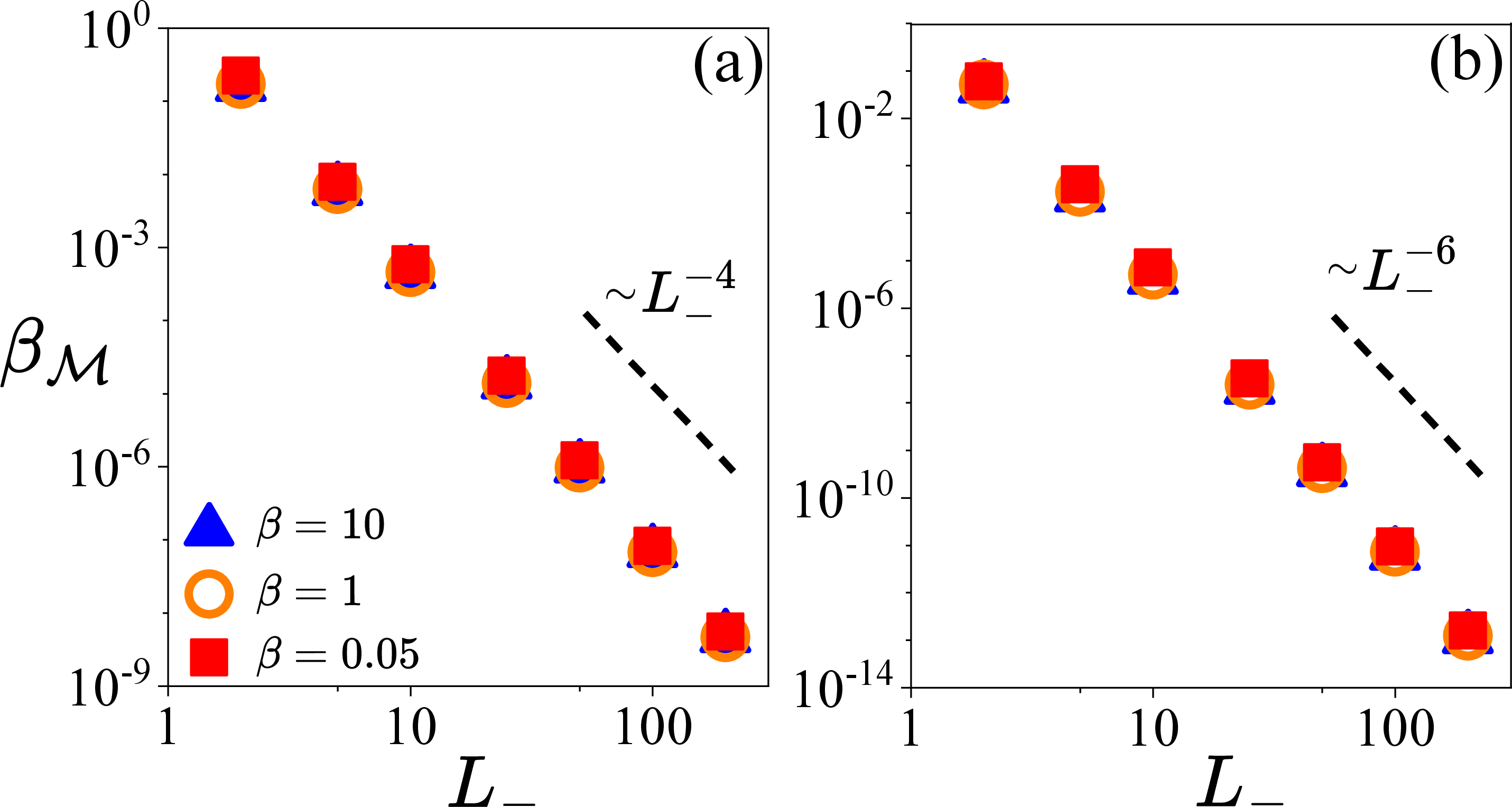
Although the formula in Eq. 8 was derived for large \(L_-\) and large \(\beta\), it is pragmatically valid down to \(L_-\) of order unity and up to (pretty warm) bath temperatures comparable to four times the barrier height. Note that at very high bath temperature (\(\beta=0.05\) in Fig. 2) the Mpemba temperature lies below the bath temperature, a phenomenon known as the inverse Mpemba effect [9]. We now propose a physical picture rationalizing our findings.

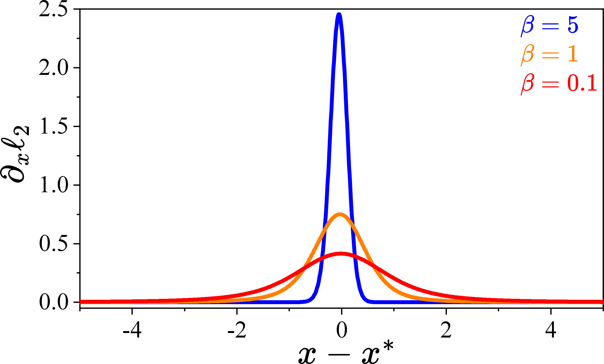
The starting point of our interpretation is a rewriting of Eq. 4 \[\frac{\partial a_2}{\partial\beta_i}=\int\text{d}x\, \partial_x\ell_2(x) \Delta U_i(x),\] where \(\Delta U_i(x)=\int_{-\infty}^x\text{d}y\, (V(y)-U_i)\pi(y,\beta_i)\). By the Sturm-Liouville theory, the function \(\ell_2(x)\) possesses exactly one zero and is monotonic (we choose \(\partial_x\ell_2(x)<0\)). For all practical purposes (see Fig. 4 in the End Matter), \(\partial_x\ell_2(x)\simeq -\delta(x-x^*)\), so that the only ingredient that matters is the sign of \(\Delta U_i(x^*)\) as a function of \(\beta_i\) (the reasoning holds as long as the width of \(\partial_x\ell_2(x)\) is smaller than the distance to the wells or walls). We must understand the thermodynamics of \(\Delta U_i(x^*)\) as a function of \(T_i\).

We find it convenient to work directly at \(L_+=+\infty\) initially. At low initial temperature \(T_i\), most of the \(\pi(x,\beta_i)\) population lies in the deepest minimum where \(U_i\simeq \min V\), so that \(\Delta U_i(x^*)>0\) (for \(y<x^*\), \(V(y)>U_i\)). This quantity will remain positive if we slightly increase the temperature, as the Boltzmann distribution starts filling the shallow well, even though \(U_i\) increases. Then we consider a much higher initial temperature \(T_i\) so that the Boltzmann distribution now feels the left wall. The distribution lowers and flattens, and begins to extend into the right wing. The contribution of \(V\) (bounded to the left) is eventually overtaken by \(U_i\) (which grows without bound to infinity as \(T_i\to\infty\)), making \(\Delta U_i(x^*)\) negative. In terms of population, since \(\Delta U_i(x^*)=T_i^2{\partial p_-}/{\partial T_i}\), we see that as \(T_i\) increases, what causes the Mpemba effect is the transfer of the probability from the left side to the right one where it can expand. Without such a wall to the left, the population would keep increasing on that side, hence killing the Mpemba effect. Now, let us insert a hard boundary to the right of the deep well. If the latter is placed too close to the minimum, the population reversal cannot occur, and \(a_2\) is monotonic. Still, if, on the contrary, it is placed sufficiently far from the well, in such a way that, as \(T_i\) increases, the Boltzmann distribution can sample the population in the vicinity of the left wall beforehand, then there must exist a Mpemba effect. Beyond the low-temperature regime, the emergence of the Mpemba effect is still driven by the population transfer, which is in turn driven by the presence of a wall. Moreover, this mechanism is valid for single-well potentials and symmetric double-well potentials as well [51].

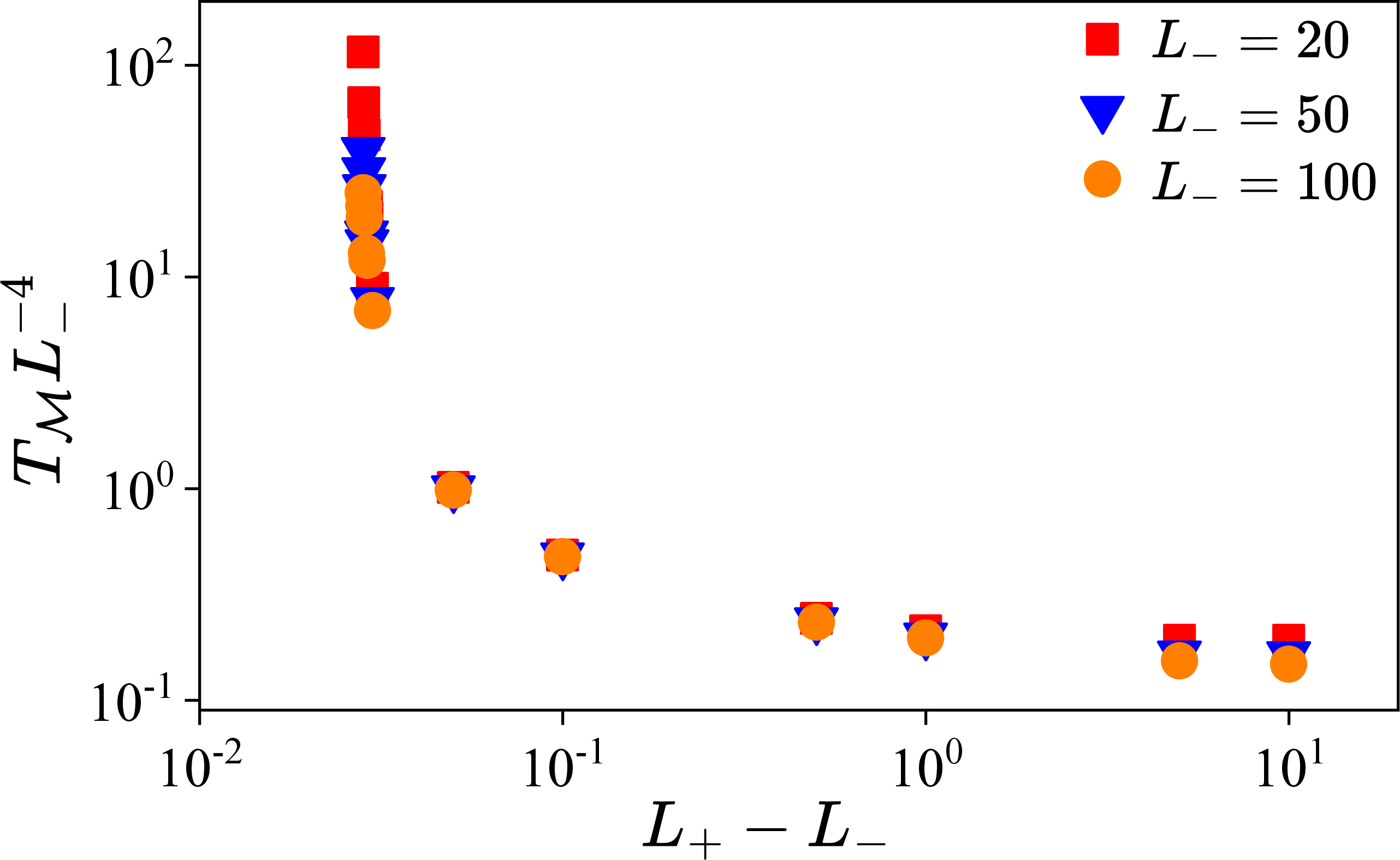
This analysis of the effect of a wall to the right, which is consistent with Eq. 7 , can also be explored numerically, as shown in Fig. 3 for a quartic potential. The rescaled Mpemba temperature \(T_{\mathcal{M}}L_{-}^{-4}\) is shown as a function of the distance between the two walls, \(L_+-L_-\). As the right wall gets closer, \(T_{\mathcal{M}}\) increases and eventually diverges, signaling the disappearance of the Mpemba effect. For large \(L_+-L_-\), the Mpemba temperature is independent of \(L_+\) and is consistent with the prediction of Eq. 8 . Finally, if Pandora’s box of mathematical possibilities is open to non-analytic potentials, with asymptotic behavior differing to the right and to the left, then of course a hard wall is not a necessary condition. All that is required to observe the Mpemba effect is a steeper potential to the left than to the right, which can reverse the population as the initial temperature is increased. One can even artificially create two or more Mpemba temperatures, a mathematical curiosity illustrated in the End Matter (as already numerically observed in Malhotra2024? for two temperatures, and expanded on in [51] for an arbitrary number of temperatures) by inserting a wall to the right. If anything, this confirms that the Mpemba effect is driven by the asymptotics of the potential regardless of its inner structure, in line with our main message.

In this work, we have considered an asymmetric double-well potential that allows for the existence of a long timescale over which the Mpemba effect could be observed. We have found that the existence of a wall to the left of the shallow well is a necessary condition for the Mpemba effect to occur, and the double-well structure and the metastability play no significant role in the emergence of the Mpemba effect. We have also shown that introducing a wall to the right can be sufficient to destroy the Mpemba effect. We have rationalized our findings by showing that the Mpemba effect is driven by a population transfer as the initial temperature increases, which is in turn driven by the presence of a wall or walls. Our findings now call for a quantitative systematic study [51] of single- and double-well potentials, including cases in symmetric double-well potentials and in more than one space dimension without walls [59], and situations where \(a_2\) may not be the leading nonzero overlap, as in symmetric potentials. Since we claim that the Mpemba effect observed in experiments [4], [50] is wall-driven rather than metastability-induced, it would be very interesting to conduct new experiments to probe the importance of the high-energy shape of the optical trap. What matters for experimental walls is a steeper divergence than within the branches of the potential landscape.

Acknowledgements. In the course of this work, we have been made aware of a similar endeavor by John Bechhoefer and Siddharth Sane, with whom we had several useful exchanges that helped us clarify our message. We also thank Marija Vucelja and Apurba Biswas for several discussions. HH thanks Satoshi Takada for fruitful discussions, and was supported by JSPS KAKENHI Grant No. 26K06960. YL gratefully acknowledges the Yukawa Research Fellow, co-sponsored by the YITP and the Yukawa Memorial Foundation. TVV was supported by JSPS KAKENHI Grant Nos. JP23K13032, JP26K00022, and JP26H02015. FvW acknowledges the financial support of the ANR grant THEMA No. 20-CE30-0031-01.

Data availability.—The data are not publicly available upon publication. The data are available from the authors upon reasonable request.

Behavior of \(\ell_2(x)\): The eigenvector \(\ell_2\) of \({\mathbb{W}}^\dagger\) corresponding to \(\lambda_2\) is known to have a single node. When \(\lambda_2\) is quasi-degenerate with \(0\), which occurs at sufficiently low bath temperature, it takes the form of a step function with a smooth error-function profile; hence, its derivative is a sharply peaked function near the location of the potential barrier. We have plotted in Fig. 4 for various values of \(\beta\) the function \(\partial_x\ell_2(x)\) (normalized by the area under the peak \(\int_{-\infty}^{+\infty}\text{d}y\,\partial_y\ell_2(y)\)). The potential we used is \(V(x)=(x^2-1)^2-0.2 x\) (the wells are a distance unity from the center and the top of the barrier, and the potential barrier is also of order unity; hence \(\beta=1\) refers to a temperature of the same order as the central barrier).

Derivation of Eqs. 6 and 7 : Due to Eq. 4 , the temperature \(T_\mathcal{M}=\beta_\mathcal{M}^{-1}\), if it exists, is given by \[\langle \ell_{2}(x)V(x)\rangle_{\beta_\mathcal{M}}-\langle \ell_{2}(x)\rangle\langle V(x)\rangle_{\beta_\mathcal{M}}=0.\] At low bath temperature (with an exponentially small error in \(\beta\)), we use \(\ell_2(x)\simeq\theta(x^*-x)\), hence \[U_{-}p_{-}-p_{-}(U_{-}p_{-}+U_{+}p_{+})=0 ,\] where \(U_{\pm}\) and \(p_{\pm}\) are defined by \[\label{eq:pandE}\begin{align} U_{\pm}:=&\pm\frac{1}{p_{\pm}}\int_{x^*}^{\pm\infty} \text{d}x\,V(x)\pi(x,\beta_{i}),\\ p_{\pm}:=&\pm\int_{x^*}^{\pm\infty} \text{d}x\,\pi(x,\beta_{i}) , \end{align}\tag{9}\] and by convention, \(V(x)=+\infty\) for \(x<-L\) and \(x>L_+\). Then the Mpemba temperature solves \[U_{-}=U_{+}.\] The potential we consider can be written as \[V(x)=v_{m}(x-x^*)^{m}+\sum_{k=0}^{m-1}v_{k}(x-x^*)^{k} ,\] and it verifies \[\begin{align} (x-x^*)V'(x)=&mV(x)-\sum_{k=0}^{m-1}(m-k)v_{k}(x-x^*)^{k}. \end{align}\] By using the above identity and an integration by parts in Eq. 9 , we can get \[\begin{align} Z(\beta_i)p_{-}=&(L_{-}+x^*)\text{e}^{-\beta_{i} V(-L_-)}+\beta_{i}mU_{-}Z(\beta_i)p_{-}\\&-\beta_{i}\sum_{k=0}^{m-1}(m-k)v_{k}\int_{-L_-}^{x^*}\text{d}x\,(x-x^*)^{k}\text{e}^{-\beta_{i} V(x)}, \end{align}\] and a similar expression holds for \(p_+\). Thus we obtain

\[\begin{align} U_{-}=&\frac{1}{m\beta_{i}}+\frac{\sum_{k=0}^{m-1}(m-k)v_{k}\int_{-L_-}^{x^*}\text{d}x\,(x-x^*)^{k}\text{e}^{-\beta_{i} V(x)}}{m Z(\beta_i)p_{-}}\\ &-\frac{(L_{-}+x^*)\text{e}^{-\beta_i V(-L_-)}}{m\beta_i Z(\beta_i)p_{-}},\\ U_{+}=&\frac{1}{m\beta_{i}}+\frac{\sum_{k=0}^{m-1}(m-k)v_{k}\int_{x^*}^{L_{+}}\text{d}x\,(x-x^*)^{k}\text{e}^{-\beta_{i} V(x)}}{mZ(\beta_i)p_{+}}\\ &-\frac{(L_{+}-x^*)\text{e}^{-\beta_i V(L_+)}}{m\beta_i Z(\beta_i)p_{+}}. \end{align}\] For large enough \(L_\pm\), the condition \(U_{-}=U_{+}\) leads to \[\frac{L_-\text{e}^{-\beta_{{\mathcal{M}}} V(-L_-)}}{m\beta_{{\mathcal{M}}}p_{-}}-\frac{L_+\text{e}^{-\beta_{{\mathcal{M}}} V(L_+)}}{m\beta_{{\mathcal{M}}}p_{+}} =\sum_{k=0}^{m-1}\frac{m-k}{m}v_{k}\Delta\langle x^{k}\rangle,\] where \(\Delta\langle x^{k}\rangle\) is defined as \[\Delta\langle x^{k}\rangle=\langle x^{k}\rangle_{+}-\langle x^{k}\rangle_{-}\] with \[\begin{align} \langle x^{k}\rangle_{+}&=\frac{\int_{x^*}^{\infty}\text{d}x\,(x-x^*)^{k}\text{e}^{-\beta_{{\mathcal{M}}} V(x)}}{p_{+}} ,\\ \langle x^{k}\rangle_{-}&=\frac{\int_{-L_-}^{x^*}\text{d}x\,(x-x^*)^{k}\text{e}^{-\beta_{\mathcal{M}} V(x)}}{p_{-}} . \end{align}\] Our task now is to determine the order of \(\Delta\langle x^{k}\rangle\). In the following, we discuss the large \(L_-\) limit, and we anticipate that the regime of interest is the high-temperature one with small \(\beta_{\mathcal{M}}\), yet with \(\beta_{\mathcal{M}}V(-L_-)\gg 1\). In this limit, we have \[\begin{align} p_-&\simeq M_{0}-\frac{1}{m\beta_{\mathcal{M}}L_-^{m-1}}\text{e}^{-\beta_{\mathcal{M}} L_-^{m}}, \end{align}\] where \(M_{k}=\int_{0}^{\infty}\text{d}x\,x^{k}\text{e}^{-\beta_{{\mathcal{M}}} x^{m}}\). In addition we see that \(M_{k}\sim \beta_{\mathcal{M}}^{-(k+1)/m}\). For the right and left sides, respectively, we have \[\begin{align} &\langle x^{k}\rangle_{+}\sim \frac{M_{k}}{M_{0}},\,\,\langle x^{k}\rangle_{-}\sim (-1)^k\frac{M_{k}}{M_{0}}. \end{align}\] We thus arrive at \[\Delta\langle x^{k}\rangle\sim\begin{cases} \beta_{i}^{-k/m}&~\text{for odd}~k,\\ 0&~\text{for even}~k, \end{cases}\] which suggests that only the highest odd term \(k=k^*\) needs to be considered (this is \(k^*=m-1\) if \(v_{m-1} \neq 0\)). Therefore, we have \[\label{eq:moment} \frac{L_-e^{-\beta_{\mathcal{M}} L_-^{m}}}{m\beta_{\mathcal{M}}\beta_{\mathcal{M}}^{-1/m}}-\frac{L_+\text{e}^{-\beta_{\mathcal{M}} L_+^{m}}}{m\beta_{\mathcal{M}}\beta_{\mathcal{M}}^{-1/m}}\sim \beta_{\mathcal{M}}^{-k^*/m},\tag{10}\] which establishes \[\begin{align} \beta_{\mathcal{M}}\simeq&(m-k^*)\frac{\ln (\text{const}\,L_-)}{L_-^m}\\ &+\frac{1}{L_-^m}\ln\left(1-\frac{L_+}{L_-}\text{e}^{-\beta_{\mathcal{M}}(L_+^m-L_-^m)}\right), \end{align}\] irrespective of whether \(k^*=m-1\) or a smaller integer.
A mathematical curiosity: If the analyticity assumption is further relaxed, then, mostly as a mathematical game, one can artificially construct a potential that not only displays a Mpemba effect without the need for a hard wall (it only takes a steeper divergence), but also exhibits two (or more) Mpemba temperatures. 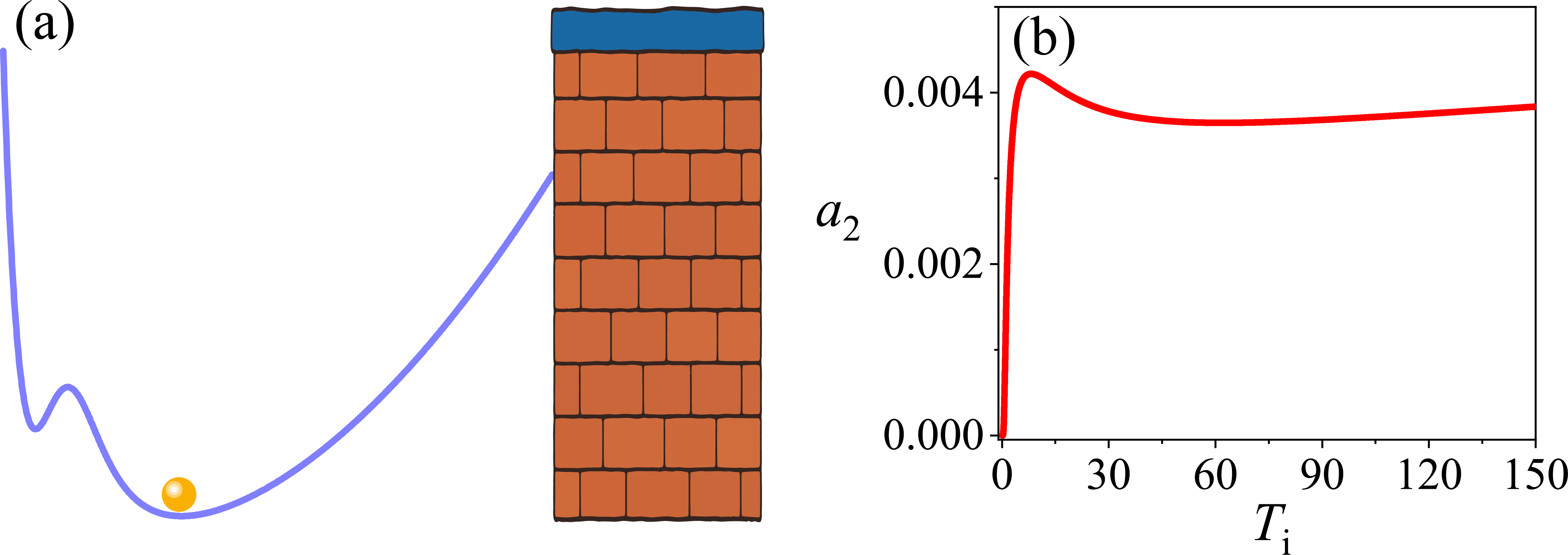Here, we adopt the choice \[\label{eq:Vnona} V(x)=\left\{ \begin{array}{l} x^4-2x^2~~\text{for}~~x<0,\\ \dfrac{x^4}{1+a x^2}-2 x^2~~\text{for}~~x>0.\end{array} \right.\tag{11}\] The left asymptotics \(x^4\) is steeper than the right asymptotics \(x^2\), which leads to the existence of a Mpemba effect. In addition, if a hard(er) wall is now inserted to the right, a secondary population inversion will occur, and a second Mpemba temperature exists. The numerical illustration of this phenomenon is provided in Fig. 5.

Similar phenomena have been observed in Ref. Degunther2022?. Here, we explain the underlying physics. Based on this mechanism, one can construct a potential with an arbitrary number of Mpemba temperatures even in single-well potentials (see the longer version [51] for details).

References↩︎