Self-supervised pre-training, two-stage \(M\)-estimation, Riemannian CLT.

1 Introduction↩︎

Self-supervised pre-training has emerged as a powerful paradigm for learning representations from large corpora of unlabeled data, which are subsequently adapted to downstream tasks via fine-tuning. This approach has achieved striking empirical success across a wide range of domains in modern machine learning. For instance in computer vision, a growing body of contrastive, masked reconstruction, and self-distillation methods [1]–[9] have demonstrated that high-quality features can be learned without manual annotation and transferred effectively across tasks. More broadly, large language models and vision-language models trained on massive unlabeled or weakly labeled corpora have shown that pre-training can endow models with general-purpose capabilities that substantially reduce the amount of labeled data required for downstream adaptation [10]–[13].

Motivated by these empirical advances, a growing body of theoretical work has begun to investigate self-supervised pre-training, including contrastive learning and other variants, from a statistical perspective [14]–[21]. Despite the varying problem setups, loss functions, and structural assumptions in these works, a central question across much of this literature is: when does the two-stage pipeline of pre-training on unlabelled data followed by fine-tuning on downstream task data provably outperform training from scratch on the downstream data alone? A closely related question involves the marginal value of pre-training data: when is the downstream task error fundamentally bottlenecked by the amount of labeled fine-tuning data, so that additional pre-training samples yield diminishing improvement for downstream task performance?

While recent works have made some progress towards answering these questions, we still lack an instance-optimal theory that precisely characterizes the role of pre-training loss, data distribution, and representation properties in downstream task performance. Indeed, much of the existing theory focuses on sufficient conditions and upper bounds, leaving open the question of how sharply current rates capture true behavior. Moreover, available results are typically not instance-adaptive: they do not explicitly reflect the interaction between the specific pre-training and fine-tuning distributions, losses, models, and representation structure. Contrast this to standard supervised learning, where classical \(M\)-estimation theory provides instance-specific asymptotic characterization of the excess risk; these bounds then serve as a benchmark for deriving sharp non-asymptotic results [22]–[24].

1.0.0.1 Our contribution.

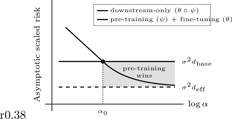
In this paper, we take a step towards bridging this gap by developing an asymptotic theory of self-supervised pre-training followed by fine-tuning with linear regression, in the joint limit of pre-training and fine-tuning data. Let \(\alpha := m/n\) denote the ratio of pre-training samples to downstream labeled samples. Our main result shows that the scaled downstream excess risk of the two-stage estimator decomposes into two leading contributions: an intrinsic fine-tuning term, corresponding to well-specified least-squares regression on the limiting representation, and a pre-training interaction term that decays as \(1/\alpha\) (see 1). Thus, as the amount of pre-training data grows relative to downstream data, the pre-training interaction term vanishes, and the risk approaches the well-specified linear regression floor. Importantly, our result identifies a precise threshold characterization (i.e., \(\alpha > \alpha_0\)) where pre-training plus fine-tuning provides strict improvement over a downstream-only baseline. Applying our main result to several case studies—including pre-training with a spectral loss, a latent factor model, and a Gaussian mixture model—illuminates substantial gaps in problem-specific factors in prior art.

A key technical challenge which arises in our analysis is that pre-training estimators are often identifiable only up to a group symmetry, which complicates the direct application of two-stage \(M\)-estimation theory [25], [26]. We address this challenge for a general pre-training loss that learns a representation used in downstream linear regression. We first establish asymptotic normality of the intrinsic pre-training representation by building on recent results in Riemannian \(M\)-estimation [27]. We then link pre-training and downstream regression together via a key conceptual step that identifies structural conditions on the learned features that ensure orbit-invariance of the downstream predictor. Our general proof strategy should be broadly applicable beyond analyzing self-supervised pre-training pipelines, and we discuss future extensions in the conclusion.

2 Related Work↩︎

Our work draws on ideas from self-supervised learning, the asymptotic theory of two-stage estimators, and Riemannian \(M\)-estimation. We defer a more comprehensive discussion of related work to 8, and focus here on the prior work most directly relevant to our contributions.

Most related to our work are [18], [20], [28]. First, [18] studies a VICReg-style [29] pre-training loss combined with downstream RKHS regression. They control the downstream test risk by the (scaled) pretrain loss, which they bound using Rademacher complexity arguments. While their downstream RKHS setup is more flexible, our analysis holds for more general pre-training losses. Next, [20] combine MLE pre-training with ERM fine-tuning. Their \(\kappa\)-informative condition shares high-level similarity with our goal of quantifying invariance in pre-training; however, the details differ substantially from our geometric approach. Finally, [28] study downstream error through the lens of RKHS approximation, showing that downstream error is influenced by two key terms: (a) the complexity of the RKHS induced by the augmentation distribution, and (b) how well the pre-trained encoder approximates the induced augmentation RKHS. In the aforementioned works, whether or not the upper bounds achieve optimal dependence on problem-specific constants is left open. In 6, we show non-trivial gaps between the upper bounds provided by [18], [20] and those that arise from our asymptotic analysis in several settings.¹

3 Problem Formulation↩︎

Let \(\mu_{\mathrm{pre}}\) and \(\mu_{\mathrm{down}}\) be probability measures on input spaces \(\mathcal{Z}\) and \(\mathcal{X}\), respectively. We consider two training datasets: (i) a pre-training dataset \(D_{\mathrm{pre}}^{(m)} \mathrel{\vcenter{:}}= \{ z_j \}_{j=1}^{m}\), where \(z_j \stackrel{\mathrm{i.i.d.}}{\sim} \mu_{\mathrm{pre}}\), and (ii) a downstream dataset \(D_{\mathrm{down}}^{(n)} \mathrel{\vcenter{:}}= \{ (x_i, y_i) \}_{i=1}^{n}\), where \((x_i,y_i) \stackrel{\mathrm{i.i.d.}}{\sim} (X,Y)\) and \(X \sim \mu_{\mathrm{down}}\). The datasets \(D_\mathrm{pre}^{(m)}\) and \(D_{\mathrm{down}}^{(n)}\) are drawn independently. The pair \((X, Y)\) is further assumed to satisfy: \[\begin{align} Y &= f_\star(X) + \varepsilon, \qquad \mathbb{E}[\varepsilon \mid X] = 0, \qquad \sigma^2 \coloneq \mathbb{E}[\varepsilon^2 \mid X] < \infty , \label{eq:X95and95Y95pair} \end{align}\tag{1}\] for some unknown regression function \(f_\star : \mathcal{X} \mapsto \mathbb{R}\). Towards parameterizing \(f_\star\), we fix a feature dimension \(p \in \mathbb{N}_+\), and consider a differentiable representation \(\psi(x, w) \in \mathbb{R}^p\), where \(w\in\mathbb{R}^{q_0}\) is the representation parameter. For each \(w\), define the linear hypothesis class \(\mathcal{H}_w \mathrel{\vcenter{:}}= \{ f_{\theta,w} \mid \theta \in \mathbb{R}^p \}\) with \(f_{\theta,w}(x) \coloneq \langle \theta, \psi(x,w) \rangle\). We assume that \(f_\star\) in 1 is well-specified with respect to \(\mathcal{F}\mathrel{\vcenter{:}}= \bigcup_{w \in \mathbb{R}^{q_0}} \mathcal{H}_w\), i.e., \(f_\star \in \mathcal{F}\). Let \((w_\star, \theta_\star)\) denote a pair such that \(f_\star = f_{\theta_\star, w_\star}\).

3.0.0.1 Notation.

Throughout, \(L^2\mathrel{\vcenter{:}}= L^2(\mu_{\mathrm{down}})\) denotes the Hilbert space of real-valued square-integrable functions \(g:\mathcal{X}\mapsto \mathbb{R}\) with inner product \(\langle g,h\rangle \mathrel{\vcenter{:}}= \mathbb{E}_{X \sim \mu_{\mathrm{down}}}[g(X)h(X)]\). The notation \(\stackrel{d}{\rightsquigarrow}\) denotes convergence in distribution, and \(\xrightarrow{\mathbb{P}}\) denotes convergence in probability. The set \(B_d(w, r) \coloneq \{ w \in \mathbb{R}^d \mid \lVert w \rVert \leqslant r \}\) denotes the closed \(\ell_2\)-ball of radius \(r\) in \(\mathbb{R}^d\); we drop the subscript \(d\) when the dimension is implicit. The set \(O(p)\) denotes the orthogonal group \(O(p) \coloneq \{ Q \in \mathbb{R}^{p \times p} \mid Q^\top Q = QQ^\top = I \}\). Finally, \((\cdot)^+\) denotes the Moore-Penrose pseudo-inverse for a matrix.

3.1 Pre-training Loss, Downstream Least-Squares Estimation, and Final Test Risk↩︎

3.1.0.1 Pre-training objective.

Let \(\ell_{\mathrm{pre}}:\mathbb{R}^{q_0}\times\mathcal{Z}\mapsto\mathbb{R}\) denote a pre-training loss which is twice continuously differentiable with respect to \(w\) for almost every \(Z\), and let \(L_{\mathrm{pre}}(w)\mathrel{\vcenter{:}}= \mathbb{E}_{Z\sim\mu_{\mathrm{pre}}}\big[\ell_{\mathrm{pre}}(w;Z)\big]\) denote the corresponding population-level pre-training loss. The pre-training stage solves: \[\begin{align} \hat{w}_m \in \mathop{\mathrm{arg\min}}_{w\in\mathbb{R}^{q_0}}\hat{L}_{\mathrm{pre}}(w;D_{\mathrm{pre}}^{(m)}) := \frac{1}{m}\sum_{j=1}^m \ell_{\mathrm{pre}}(w;z_j). \label{eq:pretrain95estimator} \end{align}\tag{2}\] Our notation deliberately abstracts away the specific form of the pre-training loss; the analysis applies broadly to standard contrastive and representation-learning losses used in practice.

3.1.0.2 Downstream estimation.

The downstream estimator uses both the pre-trained parameter \(\hat{w}_m \in \mathbb{R}^{q_0}\) and the downstream training data \(D_{\rm down}^{(n)}\) to compute:² \[\begin{align} \hat{\theta}_{m,n} \in \mathop{\mathrm{arg\min}}_{\theta \in \mathbb{R}^p} \hat{L}_{\mathrm{down}}(\theta; \hat{w}_m, D_{\mathrm{down}}^{(n)})\coloneq \frac{1}{n}\sum_{i=1}^n \bigl(y_i-\langle \theta,\psi(x_i,w)\rangle\bigr)^2 . \label{eq:downstream95estimator} \end{align}\tag{3}\] The resulting predictor for the downstream task is then \(\hat{f}_{m,n}(\cdot) \coloneq \langle \hat{\theta}_{m,n}, \psi(\cdot,\hat{w}_m) \rangle \in \mathcal{H}_{\hat{w}_m}\).

3.1.0.3 Final test risk.

Let \((X_{\mathrm{new}},Y_{\mathrm{new}})\) be an independent test pair with the same distribution as \((X,Y)\) (cf. 1 ). We focus on a conditional notion of test-time risk that conditions on the realized pre-training dataset and downstream design, while still averaging over downstream label noise. Specifically, write \(X_{1:n} \coloneq (X_1,\dots,X_n)\) and define the (conditional) test-time risk: \[\begin{align} R(D_{\mathrm{pre}}^{(m)},X_{1:n}) \mathrel{\vcenter{:}}= \mathbb{E}[\bigl(Y_{\mathrm{new}}-\hat{f}_{m,n}(X_{\mathrm{new}})\bigr)^2 \,|\,D_{\mathrm{pre}}^{(m)},\,X_{1:n}]. \label{eq:main95risk95cond} \end{align}\tag{4}\] With this notation in place, the main goal of this work is the following asymptotic characterization.

3.1.0.4 Interpreting the distributional limit 5 .

From 5 , several important implications follow. By Fatou’s lemma, we have the lower bound \(\mathbb{E}[ \mathcal{E}_\alpha ] \leqslant\lim_{m,n} \mathbb{E}[ \mathcal{E}_{m,n} ]\) (here, \(\lim_{m,n}\) is understood as \((m,n) \to \infty\) with \(m/n\to \alpha\)), which gives statistical lower bounds on the downstream performance. If the sequence \(\{ \mathcal{E}_{m,n} \}_{m,n}\) can be shown to be uniformly integrable, then this lower bound can be upgraded to equality, which yields an exact characterization of the asymptotic excess risk in expectation. Absent uniform integrability, we can still compute exact asymptotic high-probability upper bounds: since \(\mathbb{P}( \mathcal{E}_\alpha \geqslant t ) = \lim_{m,n} \mathbb{P}( \mathcal{E}_{m,n} \geqslant t )\) for any \(t > 0\) (assuming \(\mathcal{E}_\alpha\) is a continuous distribution), letting \(t(\delta)\) be such that \(\mathbb{P}( \mathcal{E}_\alpha \geqslant t(\delta)) = \delta\), we have that \(\mathbb{P}( \mathcal{E}_{m,n} \geqslant t(\delta) ) = \delta + o_{m,n}(1)\). In this work, we do not show uniform integrability, as this generally requires additional small-ball assumptions [30] on the features, which are not actually needed for 5 to hold (cf. [rem:fully-avg-risk]).

The risk definition 4 takes the conditional expectation over the randomness in \((X_{\mathrm{new}},Y_{\mathrm{new}})\) and over the downstream label noise in \(D_{\mathrm{down}}^{(n)}\) (i.e., over \((Y_1,\dots,Y_n)\) conditional on \(X_{1:n}\)), holding fixed \(D_{\mathrm{pre}}^{(m)}\) and \(X_{1:n}\). This is intentional, as it allows the limit analysis to focus on the interaction between the pre-train and fine-tune covariates \((D^{(m)}_{\mathrm{pre}}, X_{1:n})\); see 13.3 for more discussion.

4 Symmetries of the Two-Stage Pipeline↩︎

3.1 defines a two-stage \(M\)-estimation procedure via 2 and 3 , which in principle can be analyzed using the standard toolkit for classical \(M\)-estimation: consistency, asymptotic normality, and delta-method expansions [31]. However, a crucial technical hurdle is that many pre-training objectives are invariant under symmetries, i.e., there exists a compact Lie group \(G\) acting smoothly on feature parameters \(\mathbb{R}^{q_0}\) such that \[\begin{align} \ell_{\mathrm{pre}}(g \cdot w;z) = \ell_{\mathrm{pre}}(w;z) ,\; \text{for all } g \in G,\;w \in \mathbb{R}^{q_0},\;z \in \mathcal{Z}. \label{eq:pretrain95group95invariance} \end{align}\tag{6}\] Concretely, consider a simple setting where \(\mathcal{Z} = \mathbb{R}^d\) and we aim to learn a linear representation \(\psi(x, A) = A x\) with \(A \in \mathbb{R}^{p \times d}\) in pre-training. Now, consider any family of pre-training losses (e.g., contrastive losses such as SimCLR [1], [4]) that act on this representation through a similarity measure \(\mathrm{sim}(x, x'; A) := \langle \psi(x, A), \psi(x', A) \rangle\). This similarity measure, and hence the pre-training loss, is invariant under any orthogonal transform \(Q \in O(p)\), i.e., \(\mathrm{sim}(x, x'; A) = \mathrm{sim}(x, x'; QA)\).

Consequently, population minimizers are typically not identifiable: if \(w\) minimizes \(L_{\mathrm{pre}}(w)\), then the entire orbit \([w] \mathrel{\vcenter{:}}= \{ g \cdot w\mid g \in G \}\) does as well. This lack of identifiability rules out both consistency and asymptotic normality for the direct parameter \(w\). One of our key contributions is to make explicit the types of symmetry encountered in self-supervised pre-training—in a way that remains compatible with asymptotic analysis—utilizing concepts from Riemannian geometry and smooth manifolds [32].

4.1 Manifold Identifiability and Asymptotic Normality↩︎

The invariance 6 implies that the intrinsic parameter is an orbit \([w]\), i.e., an element of the quotient \(\mathbb{R}^{q_0}/G\). Rather than work directly with the quotient, we represent it through a descriptor map \(D:\mathbb{R}^{q_0}\mapsto\mathbb{R}^q\) that is (a) constant along orbits: \(D(g\cdot w)=D(w)\) for all \(g\in G,\;w\in\mathbb{R}^{q_0}\), and (b) separates orbits locally around \(w_\star\): \(\exists r>0\) such that for \(w,w'\in B(w_\star,r)\), we have \(D(w)=D(w')\) iff \(w' \in [w]\). We will also require that \(\mathcal{M}\coloneq D\bigl(B(w_\star,r')\bigr)\subset\mathbb{R}^q\), for some \(0 < r' \leqslant r\), is a well-defined \(C^2\) embedded sub-manifold with \(\Omega_\star \coloneq D(w_\star)\) in its interior; 5 details the minimal assumptions needed for \(D\) to satisfy these requirements. We endow \(\mathcal{M}\) with the Riemannian metric inherited from the ambient Euclidean space \(\mathbb{R}^q\). Accordingly, for \(\Omega\in\mathcal{M}\) we write \(T_\Omega\mathcal{M}\) for the tangent space, and denote by \(\mathrm{grad}\,L_{\mathrm{pre}}(\Omega)\in T_\Omega\mathcal{M}\) and \(\mathrm{Hess}\,L_{\mathrm{pre}}(\Omega):T_\Omega\mathcal{M}\mapsto T_\Omega\mathcal{M}\) the Riemannian gradient and Hessian of \(L_{\mathrm{pre}}\) restricted to \(\mathcal{M}\).

4.1.0.1 Identifiability in descriptor coordinates.

We will study pre-training through the induced estimator \(\hat{\Omega}_m\mathrel{\vcenter{:}}= D(\hat{w}_m)\), rather than through the non-identifiable representative \(\hat{w}_m\) itself. We start by assuming the population minimizer \(\Omega_\star :=\mathop{\mathrm{arg\min}}_{\Omega\in D(\mathbb{R}^{q_0}) \mathrel{\vcenter{:}}= \{D(w)\mid w\in\mathbb{R}^{q_0}\}} L_{\mathrm{pre}}(\Omega)\) is unique in the descriptor space. We overload the notation \(L_{\mathrm{pre}}(\Omega)\mathrel{\vcenter{:}}= L_{\mathrm{pre}}(w)\) for any \(w\in D^{-1}(\Omega)\), which is well-defined as \(L_{\mathrm{pre}}\) is \(G\)-invariant (cf. 6 ). Since \(\Omega_\star\) is unique and lies in the interior of the manifold \(\mathcal{M}\), we have \(\mathrm{grad}\,L_{\mathrm{pre}}(\Omega_\star)=0\). To obtain local quadratic control and a well-posed second-order expansion on \(\mathcal{M}\), we further assume that \(\mathrm{Hess}\,L_{\mathrm{pre}}(\Omega_\star)\) is invertible on the tangent space: there exists \(\mu>0\) such that for all \(v \in T_{\Omega_\star} \mathcal{M}\), \(\big\langle v,\;\mathrm{Hess}\,L_{\mathrm{pre}}(\Omega_\star)\,v \big\rangle \geqslant \mu\,\|v\|^2\).

4.1.0.2 Asymptotic normality on the descriptor manifold.

Let \(H_\star \coloneq \mathrm{Hess}\,L_{\mathrm{pre}}(\Omega_\star)\) denote the Hessian of the population pre-training loss, and let \(\Sigma_\star \coloneq \mathbb{E}\!\left[ \mathrm{grad}\,\ell_{\mathrm{pre}}(\Omega_\star;Z) \mathrm{grad}\,\ell_{\mathrm{pre}}(\Omega_\star;Z)^\top \right]\) denote the Fisher Information of the pre-training score. Writing \(v_m \mathrel{\vcenter{:}}=\log_{\Omega_\star}(\hat{\Omega}_m)\in T_{\Omega_\star}\mathcal{M}\), then under the regularity conditions stated formally in 4, we show ([thm:riem95mestimator95clt]) that: \[\begin{align} \sqrt m\,v_m \;\stackrel{d}{\rightsquigarrow}\; \mathcal{N}\!\left(0,\;H_\star^{-1}\Sigma_\star H_\star^{-1}\right) \qquad\text{in }T_{\Omega_\star}\mathcal{M}. \label{eq:manifold95dist95conv} \end{align}\tag{7}\] 7 is the manifold analogue of classical asymptotic normality for the pre-training estimator. It follows by extracting out the asymptotic normality argument from [27], replacing geodesic convexity assumptions with local smooth regularity conditions that apply to our pre-training setting; see 11.4 for a detailed discussion.

4.2 Relating Pre-training and Downstream Estimation via Orthogonal Equivariance↩︎

As detailed in 3, the downstream stage depends on the pre-training stage through the representation map \(\psi(\cdot,\hat{w}_m)\). However, as the symmetry in 6 precludes \(\hat{w}_m\) from asymptotically converging to a fixed optimal parameter value, this implies that the convergence of both \(\psi(\cdot, \hat{w}_m)\) and its induced linear hypothesis class \(\mathcal{H}_{\hat{w}_m}\) are not well-defined without extra structure. To handle this issue, we assume that the symmetry of pre-training is compatible with downstream prediction in the sense that the induced hypothesis class is orbit-invariant: \(\mathcal{H}_{g\cdot w}=\mathcal{H}_w\) for all \(g\in G,\;w\in\mathbb{R}^{q_0}\). This condition expresses that different representatives within the same orbit \([w]\) yield the same family of predictors. However, this assumption alone is insufficient: when the OLS minimizer 3 is not unique, different pre-training parameters \(\hat{w}_m\) within the same orbit can still lead to different minimum-norm choices. Therefore, we introduce the following condition, which we call orthogonal equivariance to address this issue. Specifically, we assume there exists a homomorphism \(\rho:G\mapsto O(p)\) (i.e., \(\rho(g_1 g_2)=\rho(g_1)\rho(g_2)\) for all \(g_1,g_2 \in G\)) such that \[\begin{align} \psi(x,g\cdot w)=\rho(g)\,\psi(x,w), \; \text{for all }g\in G,\;w\in\mathbb{R}^{q_0},\;x\in\mathcal{X}. \label{eq:psi95orth95equiv} \end{align}\tag{8}\] Under condition 8 , since different representatives \(w\) in the same orbit correspond to orthogonal coordinate changes in feature space, the corresponding OLS minimizer will be constant on the orbit. Assume the orthogonal equivariance condition 8 . Fix a downstream dataset \(D_{\mathrm{down}}^{(n)}\) and a parameter \(w\in\mathbb{R}^{q_0}\). Let \(\hat{\theta}_w\) denote the minimum norm solution of the downstream OLS 3 with features \(\psi(\cdot, w)\), and \(\hat{f}_w(x)\mathrel{\vcenter{:}}= \langle \hat{\theta}_w,\psi(x,w)\rangle\). Then for every \(g\in G\), \(\hat{f}_{g\cdot w}(\cdot)=\hat{f}_w(\cdot)\).

[lem:orbit95invariant95min95norm] states that under 8 , an intrinsic downstream feature map can be naturally defined on the orbit \([w]\) of each parameter. To see this, since \(D\) is constant on orbits, it induces a map on the quotient, and we use the descriptor \(\Omega:=D(w)\) as a representative coordinate for the orbit \([w]\). Then, [lem:orbit95invariant95min95norm] implies the feature map \(\phi(x,\Omega)\mathrel{\vcenter{:}}= \psi\bigl(x,s(\Omega)\bigr)\) is intrinsic for \(\Omega \in \mathcal{M}\), where \(s:\mathcal{M}\cap B(\Omega_\star,r'')\mapsto B(w_\star,r')\) is a \(C^2\) local lift for some \(r''>0\), satisfying \(D(s(\Omega))=\Omega\).³

5 Main Result: Asymptotic Behavior of the Test Risk↩︎

We now state our main result, which characterizes the joint-sample asymptotic behavior of the conditional test risk 4 . We first introduce the operator notation used in the theorem statement.

5.1 Operator Notation and First-Order Residual Expansions↩︎

Let \(\mathcal{H}_\Omega\subset L^2\) denote the downstream function class induced by \(\phi(\cdot,\Omega)\) and \(\Pi_\Omega\) be the population \(L^2\)-orthogonal projector onto \(\mathcal{H}_\Omega\). Define the residual \(e_\Omega \coloneq (I-\Pi_\Omega)f_\star\) and \(\mathrm{Rep}(\Omega)\coloneq\|e_\Omega\|_{L^2}^2\). Note that under our well-specified setting \(f_\star \in \mathcal{F}\), \(e_{\Omega_\star}=0\). Define the effective dimension \(d_{\mathrm{eff}}(\Omega) \mathrel{\vcenter{:}}= \mathrm{dim}(\mathcal{H}_\Omega) = \mathop{\mathrm{rank}}(\Sigma(\Omega))\) for a descriptor \(\Omega\).

The pretraining contribution is controlled by the first-order behavior of the residual \(e_\Omega\) around \(\Omega_\star\). We assume that this residual admits a first-order expansion in normal coordinates, i.e., there exists a bounded linear map \(\mathcal{L}:T_{\Omega_\star}\mathcal{M} \mapsto L^2\) such that \(e_{\exp_{\Omega_\star}(v)} = \mathcal{L}(v)+o(\lVert v \rVert)\) in \(L^2\). 14.2 gives sufficient structural conditions for such an expansion, which we now highlight. Let \(N_\star\coloneq\ker(T_{\Omega_\star})\), \(E_\star:=N_\star^\perp\), \(\mathcal{A}_v:=\operatorname{Im}\left(T_{\exp_{\Omega_\star}(v)}|_{E_\star}\right)\) and define the activated null-direction span: \[\mathcal{B}_v := \operatorname{Im}\left( (I-\Pi_{\mathcal{A}_v})T_{\exp_{\Omega_\star}(v)}|_{N_\star} \right).\] We assume that there exists a stable limiting span of null directions (9), meaning that the projectors \(\Pi_{\mathcal{B}_v}\) converge in operator norm to a limiting projector \(\Pi_{\mathcal{B}_0}\), with \(\mathcal{B}_0\subseteq \mathcal{H}_{\Omega_\star}^{\perp}\). Define the active dimension \(d_{\mathrm{act}}(\Omega_\star)\coloneq \dim\big(\mathcal{H}_{\Omega_\star}\oplus \mathcal{B}_0\big)\), which denotes the total limiting downstream degrees of freedom: the original effective dimension \(d_\mathrm{eff}(\Omega_\star)\) plus the activated null directions. Let \(\Pi_\star\coloneq\Pi_{\Omega_\star}\), and let \(\theta_\star\in E_\star\) denote the unique coefficient vector with \(T_{\Omega_\star}\theta_\star=f_\star\). Under these conditions, the residual linearization has the form: \[\label{eq:linear95map95interaction} \mathcal{L}(v) = -\big(I-\Pi_\star-\Pi_{\mathcal{B}_0}\big)DT_{\Omega_\star}[v]\theta_\star, \qquad v\in T_{\Omega_\star}\mathcal{M}.\tag{9}\] The projector \(I-\Pi_\star-\Pi_{\mathcal{B}_0}\) removes both the original well-specified span and the limiting active null-direction span; only the remaining first-order variation contributes to representation error. For the regular case \(\mathcal{B}_0=\{0\}\), the active and effective dimension coincide, i.e., \(d_{\mathrm{act}}(\Omega) = d_{\mathrm{eff}}(\Omega)\).

5.2 Asymptotic Behavior of the Conditional Excess Test Risk↩︎

With this first-order expansion in place, we now turn to our main object of study: the scaled excess test-risk \(\mathcal{E}_{m,n}\) in 5 , obtained by conditioning on the realized pre-training sample and downstream design, and averaging only over the downstream label noise and the test pair. Accordingly, \(\mathcal{E}_{m,n}\) is a random variable measurable with respect to the joint law \((D_{\mathrm{pre}}^{(m)},X_{1:n})\), which we take all the convergences below with respect to. The following is our main result, which characterizes the asymptotic behavior of the conditional excess test risk.

[thm:master-compatible] shows that the (scaled) conditional excess risk \(\mathcal{E}_{m,n}\) converges in distribution to a random variable with two distinct terms. The first term, \(\sigma^2 d_{\mathrm{act}}(\Omega_\star)\), is the downstream OLS degrees-of-freedom contribution on the limiting active class \(\mathcal{H}_{\Omega_\star}\oplus \mathcal{B}_0\). The second term \(\alpha^{-1} \lVert \mathcal{L}(Z) \rVert^2_{L^2}\) on the other hand captures the interaction between the pre-training loss and the downstream regression problem. As the pre-training data starts to dominate the downstream data (i.e., \(\alpha \to \infty\)), the contribution of the second term correctly vanishes. The remaining term is the downstream OLS degrees-of-freedom contribution on the limiting active class; in the regular case \(\mathcal{B}_0=\{0\}\), this reduces to the risk of well-specified OLS on \(\mathcal{H}_{\Omega_\star}\). On the other hand, when pre-training data is relatively scarce compared to downstream (i.e., \(\alpha \to 0\)), the second term is dominant in 10 , as the bias of the learned pre-training features becomes the limiting factor in the two-stage estimator. In 6, we instantiate [thm:master-compatible] on several examples to illustrate how the assumptions translate over to concrete problem instances, and how the pre-training interaction term scales in practice.

5.2.0.1 Downstream-only baseline.

To further interpret [thm:master-compatible] and the risk-crossover picture in 1, we compare to the empirical risk minimizer over \(\mathcal{F}\) using only \(D_{\mathrm{down}}^{(n)}\), in the regular case \(\mathcal{B}_0 = \{0\}\). Specifically, define \(f_n^{\mathrm{base}}\in\mathop{\mathrm{arg\min}}_{f\in\mathcal{F}}\frac{1}{n}\sum_{i=1}^n (y_i-f(x_i))^2\). For a regular realization \((\theta_\star,w_\star)\) of \(f_\star\), define \(d_{\mathrm{base}}\) as the rank of the linear map \[(\delta\theta,\delta w)\mapsto\left.\frac{\mathrm{d}}{\mathrm{d}t}\right|_{t=0}f_{\theta_\star+t\delta\theta,\;w_\star+t\delta w}.\] Thus \(d_{\mathrm{base}}\) is the dimension of the tangent space to the full downstream-only class \(\mathcal{F}\) at \(f_\star\). This should be contrasted with \(d_{\mathrm{eff}}(\Omega_\star)\), which is the local dimension of the fixed representation class \(\mathcal{H}_{\Omega_\star}\) appearing after pre-training. Assuming the standard regularity conditions for nonlinear least squares at the function level—i.e., differentiability of the parameterization, finite moments, and constant rank of the tangent map in a neighborhood of a regular realization \((\theta_\star,w_\star)\)—the downstream-only baseline has leading scaled excess-risk limit \(\sigma^2 d_{\mathrm{base}}\), whereas [thm:master-compatible] gives the two-stage limit \(\sigma^2 d_{\mathrm{eff}}(\Omega_\star)+\alpha^{-1}\|\mathcal{L}(Z)\|_{L^2}^2\). Therefore, if \(d_{\mathrm{base}}>d_{\mathrm{eff}}(\Omega_\star)\),⁴ then, under uniform integrability of the downstream-only and two-stage scaled excess risks, the two-stage procedure has smaller asymptotic risk in expectation whenever \(\alpha>\alpha_0\coloneq \frac{\mathbb{E}\|\mathcal{L}(Z)\|_{L^2}^2}{\sigma^2(d_{\mathrm{base}}-d_{\mathrm{eff}}(\Omega_\star))}\).

6 Examples↩︎

In this section, we apply our main result ([thm:master-compatible]) on a few concrete self-supervised learning examples. For each setting there are two key steps: (i) defining the minimal problem-specific structure to satisfy the assumptions of [thm:master-compatible], and (ii) calculating the instance-specific bound from 10 . Here, we describe the main setup and assumptions, deferring specific computations to the appendix. For our examples, we restrict attention to the regular case \(\mathcal{B}_0=\{0\}\). Geometrically, this rules out the activation of coefficient directions that are null at \(\Omega_\star\) under infinitesimal perturbations of the descriptor. Under Assumptions 7 and 8, this is precisely the setting in which the population projector \(\Omega\mapsto\Pi_\Omega\) is Fréchet differentiable at \(\Omega_\star\). In this case, the residual linearization is given by \[\label{eq:linear95map95interaction95zero} \mathcal{L}(v) = -D\Pi_{\Omega_\star}[v]f_\star= \big(I-\Pi_{\Omega_\star}\big)DT_{\Omega_\star}[v]f_\star, \qquad v\in T_{\Omega_\star}\mathcal{M}.\tag{11}\]

6.1 Linear Spectral Pre-training↩︎

Inspired by the problem setting considered in [18], we first consider a linear spectral contrastive objective; proofs for this case study are given in 15.

6.1.0.1 Data model.

Let \(x\in\mathbb{R}^d\) denote a generic unlabeled pre-training sample with mean zero and covariance \(\Sigma_{\mathrm{pre}}\mathrel{\vcenter{:}}= \mathbb{E}[xx^\top]\in\mathbb{R}^{d\times d}\). A positive pair consists of two augmented views \((x,x^+)\) of the same underlying instance. We define the cross-covariance matrix \(\Sigma_{\mathrm{pre}}^{+}\mathrel{\vcenter{:}}= \mathbb{E}[x^+ x^\top]\) and assume that \((x,x^+)\) is exchangeable which implies that \(\Sigma_{\mathrm{pre}}^{+}\) is symmetric. A negative sample \(x^-\) is an independent copy of \(x\), independent of \((x,x^+)\). We group the samples as \(z\mathrel{\vcenter{:}}= (x,x^+,x^-)\).

6.1.0.2 Linear features and spectral loss.

Fix a representation dimension \(k\in[d]\) and consider linear representative-level feature maps \(\psi(x,A)\mathrel{\vcenter{:}}= Ax\in\mathbb{R}^k\) for \(A\in\mathbb{R}^{k\times d}\). For any such \(A\), define the Gram matrix (descriptor) \(M_A\mathrel{\vcenter{:}}= A^\top A\in\mathbb{R}^{d\times d}\). Here, we retain the notation \(A\) for the representative parameter (corresponding to \(w\)) and write \(M\) for the Gram descriptor (corresponding to \(\Omega\)). Motivated by prior work on spectral contrastive objectives [17], we consider the following (single-negative) spectral loss and define the per-sample objective \[\begin{align} \label{eq:spec-loss-sample} \ell_{\mathrm{spec}}(A;z) &\mathrel{\vcenter{:}}= -2\,\langle \psi(x, A),\psi(x^+,A)\rangle +\langle \psi(x,A),\psi(x^-,A)\rangle^2. \end{align}\tag{12}\]

6.1.0.3 Symmetry, quotient, and descriptor.

The loss 12 depends on \(w\) only through \(M_A=A^\mathsf{T}A\). Let \(G = O(k)\) denote the group of \(k\times k\) orthogonal matrices acting on \(\mathbb{R}^{k\times d}\) by left multiplication. Then \(\ell_{\mathrm{spec}}(QA;z)=\ell_{\mathrm{spec}}(A;z)\) for all \(Q\in O(k)\) and all \(z\), and hence \(\hat{L}_{\mathrm{pre}}\) and \(L_{\mathrm{pre}}\) are invariant under this action (cf. 6 ). Moreover, the representative-level feature map is orthogonally equivariant (cf. 8 ), that is, \(\psi(x,Q\cdot A)=Q\psi(x,A)\) for all \(x\in\mathbb{R}^d\) and \(Q\in O(k)\). A natural orbit-invariant descriptor map is \(D(A)\mathrel{\vcenter{:}}= M_A=A^\mathsf{T}A\) which is constant along \(O(k)\)-orbits. On the regular regime \(\mathrm{rank}(A)=k\), the action is free, and \(D\) locally identifies nearby \(O(k)\)-orbits with nearby points in the rank-\(k\) PSD cone \(\mathcal{M}_{d,k}\mathrel{\vcenter{:}}= \{M\in\mathbb{R}^{d\times d}\mid M\succcurlyeq 0,\;\mathrm{rank}(M)=k\}\). In particular, \(\mathcal{M}_{d,k}\) is a smooth embedded submanifold of the space of symmetric matrices, and we may endow it with the induced Riemannian metric from the ambient Frobenius inner product. On a neighborhood of \(M_\star\) there exists a \(C^2\) local section \(s\) with \(s(M)^\top s(M)=M\), and we define the quotient feature map by \(\phi(x,M):=s(M)x\); see Appendix 15.1 for the construction and smoothness.

Under 1, the population descriptor minimizer \(M_\star\in\mathcal{M}_{d,k}\) exists and is unique, which leads to the following verification of the assumptions. Assume 1 and \(\mathbb{E}_{\mu_{\mathrm{pre}}}\|Z\|^{4},\mathbb{E}_{\mu_{\mathrm{down}}}\|x\|^4<\infty\). Then the linear spectral model satisfies the assumptions of [thm:master-compatible].

6.1.0.4 Concrete example.

While the limiting expression in [thm:master-compatible] admits an explicit characterization in this linear spectral model, its general form is involved. To obtain explicit closed-form expressions, we consider a simplified linear model inspired by [19]. We focus on a diagonal setting that captures the essential spectral structure while allowing for precise calculations. Assume that \(\Sigma_{\mathrm{pre}} = I_d\) and \(\Sigma_{\mathrm{pre}}^{+} = \mathop{\mathrm{diag}}(1,1/2,\ldots,1/d)\), so that the whitened cross-covariance matrix is \(C = \mathop{\mathrm{diag}}(1,1/2,\ldots,1/d)\). The top-\(k\) population representation is therefore given by the first \(k\) coordinates. We consider a linear downstream target \(f_\star(x) = \beta_\star^\top A_\star x\) where \(A_\star = [\mathop{\mathrm{diag}}(1,1/\sqrt{2},\dots,1/\sqrt{k}),0_{k\times (d-k)}]\) and \(\beta_\star = (1,\ldots,1)^\top\). This ensures that the task is realizable. We further assume the downstream data distribution satisfies \(\mu_{\mathrm{down}}=\mathcal{N}(0,I_d)\). Under the above setup, as \((m,n)\to(\infty,\infty)\) with \(m/n\to\alpha\in(0,\infty)\), \[n\Big(R(D_{\mathrm{pre}}^{(m)},X_{1:n})-\sigma^2\Big) \;\stackrel{d}{\rightsquigarrow}\; \sigma^2\,k+\frac{2}{\alpha}\,\left(\sum_{i=1}^k i(1+i^{-2}+\tau) \right)\,\chi^2_{d-k}, \quad \tau = \sum_{j=1}^k j^{-2}.\] In particular, the pre-training interaction term \(\frac{1}{m}\|\mathcal{L}(Z)\|_{L^2}^2\) scales as \(\Theta\big(\frac{k^2(d-k)}{m}\big)\) w.h.p. We compare [cor:linear-concrete] with [18]. Applied to this setup, [18] yields (ignoring \(\log{n}\) factors) that \(\mathbb{E}[\mathcal{E}_{m,n}] \lesssim \sigma^2 k + \alpha^{-1} k(d-k)\|C^{-1}A_\star^\top\beta_\star\|^2_2 \asymp \sigma^2 k + \alpha^{-1} k^3(d-k)\) (see 15.7). On the other hand, [cor:linear-concrete] implies that for large \(m,n\), \(\mathcal{E}_{m,n} \asymp \sigma^2 k + \alpha^{-2} k^2(d-k)\) w.h.p. Thus, our result improves the dependence in the second term by factor of \(k\).

6.2 Factor Model Pre-training↩︎

We next specialize our main result to the latent factor example from [20]. This setting is structurally similar to 6.1: the latent low-rank structure makes unsupervised pretraining natural, while a rotational invariance renders representation-level parameters non-identifiable. Proofs for this case study are presented in 16.

6.2.0.1 Factor model and pre-training.

Let \(x\in\mathbb{R}^d\) be generated according to the factor model \(x = A_\star h + \mu\) where \(h\sim\mathcal{N}(0,I_k)\) is a latent factor, \(\mu\sim\mathcal{N}(0,I_d)\) is independent noise, and \(A_\star\in\mathbb{R}^{d\times k}\) is an unknown full-rank factor loading matrix. We assume that \(k\ll d\). Pre-training observes \(m\) i.i.d.draws \(\{z_i\}_{i=1}^{m}\) from the same distribution as \(x\), and uses MLE to estimate the factor loading matrix, i.e., \(\ell_{\mathrm{pre}}(A; z_i) = \frac{1}{2}\left( \log\det( I_d + AA^\top ) + z_i^\top (I_d + AA^\top)^{-1} z_i \right)\).

6.2.0.2 Downstream regression.

We observe labeled samples \((x,y)\) satisfying \(y = \beta_\star^\top h + \nu\) where \(\nu\sim\mathcal{N}(0,\sigma_{\nu}^2)\) and independent of \((h,\mu)\). The downstream learner does not observe \(h\) and fits a linear predictor based on features extracted from \(x\) using the pretrained representation. Specifically, under the Gaussian factor model, the regression function is linear and admits a closed form \(f_\star(x)= \beta_\star^\top A_\star^\top (I_d + A_\star A_\star^\top)^{-1}x\). Accordingly, we can write the downstream labels as \(Y = f_\star(X) + \varepsilon\) where \(\varepsilon \mid X\sim \mathcal{N}(0,\sigma^2)\) and \(\sigma^2\coloneq\sigma_{\nu}^2 + \beta_\star^\top(I_d+A_\star A_\star^\top)^{-1}\beta_\star\).

6.2.0.3 Reduction to the linear case.

For any candidate loading matrix \(A\in\mathbb{R}^{d\times k}\) we define the representative-level feature map \(\psi(x,A)\mathrel{\vcenter{:}}= W(A) x \in \mathbb{R}^k\) with \(W(A) \coloneq A^\top(I_d+AA^\top)^{-1}\). Writing the orbit-invariant descriptor as \(M=AA^\top\in\mathcal{M}_{d,k}\) and choosing any local section \(s(M)\) with \(s(M)s(M)^\top=M\), any representative \(A\) on the same orbit can be expressed as \(A=s(M)Q\) for some \(Q\in O(k)\), which yields \(\psi(x,A)=Q^\top \phi(x,M)\) with \(\phi(x,M)\mathrel{\vcenter{:}}= s(M)^\top(I_d+M)^{-1}x\). Thus, passing from \(A\) to \(M\) removes the rotational non-identifiability. Consequently, this factor-model instance is a direct specialization of the linear example at the descriptor level, with the downstream class determined solely by the \(k\)-dimensional subspace \(\mathrm{range}(M)\). Let \(M_\star = U_\star \mathop{\mathrm{diag}}(\Sigma_\star,0_{d-k})U_\star^\top\) with \(\Sigma_\star=\operatorname{diag}(\sigma_1,\dots,\sigma_k)\) and \(U_\star=[U_1\;U_2]\), where \(U_1\in\mathbb{R}^{d\times k}\) spans \(\operatorname{range}(M_\star)\).

For the factor model example, as \((m,n)\to(\infty,\infty)\) with \(m/n\to\alpha\in(0,\infty)\), \[n\Big(R(D_{\mathrm{pre}}^{(m)},X_{1:n})-\sigma^2\Big) \;\stackrel{d}{\rightsquigarrow}\; \sigma^2\,k+\frac{1}{\alpha}\,\|(I_k+\Sigma_\star)^{-1/2}\,U_1^\top A_\star\,\beta_\star\|_2^2\,\chi^2_{d-k}.\] Compared to [20], which states that w.h.p.,⁵ \(\mathcal{E}_{m,n} \lesssim D^4 k + \alpha^{-1} D^{12} (D^4 + \sigma_{\min}^{-4}(A_\star)) d\) whenever \(m \gtrsim D^4 d\), \(n \geqslant D^4 k\) where \(D \coloneq \max\{ \lVert A_\star \rVert_{\mathrm{op}}, \lVert \beta_\star \rVert , 1 \}\) (here, we ignore all \(\log(1/\delta)\) for simplicity), we see that [cor:factor] provides a substantial improvement. In particular, it implies a sharper bound of the form \(\mathcal{E}_{m,n} \asymp (\sigma_\nu^2 + D^2) k + \alpha^{-1} D^2 (d-k)\) w.h.p. for large \(m,n\), yielding a significant improvement on the dependence of \(D\).

6.3 Gaussian Mixture Pre-training with Subspace-Aware Gating↩︎

Our final example considers unlabeled pretraining data drawn from a Gaussian mixture (MoG) with unknown centers, while the downstream predictor uses subspace-aware posterior responsibilities that depend only on a low-dimensional centered-mean subspace. This example is motivated by the latent classification models studied in e.g.[20], [21], [33], which we naturally extend to the regression setting. From a technical perspective, it also instantiates the quotient-descriptor viewpoint in a setting with discrete non-identifiability. As before, we discuss only the minimal ingredients needed to invoke [thm:master-compatible], and we defer many details to 17.

6.3.0.1 Pre-training data and loss.

Fix \(d\geqslant 1\) and \(K\geqslant 2\). Let \(U^\star=(u_1^\star,\dots,u_K^\star)\in(\mathbb{R}^d)^K\) be unknown centers and let \(\tau\sim\mathrm{Unif}([K])\). The unlabeled distribution is the MoG \(Z \mid (\tau=i) \sim \mathcal{N}(u_i^\star, I_d)\) for \(i\in[K]\). Given \(m\) i.i.d.pre-training samples \(Z_i \stackrel{\mathrm{i.i.d.}}{\sim} \frac{1}{K}\sum_{i=1}^K \mathcal{N}(u_i^\star,I_d)\), we estimate \(U^\star\) by MLE using \(\ell_{\mathrm{pre}}(U;Z) \mathrel{\vcenter{:}}= -\log(\frac{1}{K} \sum_{i=1}^K \varphi(Z-u_i))\) where \(\varphi(\cdot)\) is the density of \(\mathcal{N}(0, I)\).

6.3.0.2 Subspace-aware features.

Define the empirical mean \(\bar u(U):=\frac{1}{K}\sum_{i=1}^K u_i\) and centered second-moment matrix \(S(U):=\sum_{i=1}^K \big(u_i-\bar u(U)\big)\big(u_i-\bar u(U)\big)^\top\). Let \(r_\star:=\mathrm{rank}(S(U_\star))\) and define \(P_U\in O(d)\) to be the orthogonal projector onto the leading \(r_\star\)-dimensional eigenspace of \(S(U)\) (on the regular neighborhood where this eigenspace is well-defined); centering via \(S(U)\) removes an irrelevant global shift and isolates the effective subspace in which the mixture geometry varies. For \(U\) in the regular neighborhood, define responsibilities based on the projected mixture: \[\label{eq:ex-mog-gating} \pi_i(x;U) := \frac{\exp\!\big(\langle P_U u_i,\;P_U x\rangle-\tfrac12\|P_Uu_i\|_2^2\big)}{\sum_{j=1}^K \exp\!\big(\langle P_U u_j,\;P_U x\rangle-\tfrac12\|P_Uu_j\|_2^2\big)}, \; i\in[K].\tag{13}\] These are exactly the Bayes posteriors \(\pi_i(x;U)=\mathbb{P}_U(Z=i\mid P_U X=P_U x)\) for the projected model \(P_UX\mid (Z=i)\sim \mathcal{N}(P_Uu_i, I_{r_\star})\). Define the feature map \(\psi_U:\mathbb{R}^d\mapsto\mathbb{R}^{K(d+1)}\) by \[\begin{align} \label{eq:ex-mog-feature} \psi_U(x) := \Big( \pi_1(x;U) P_U (x-u_1),\, \pi_1(x;U),\; \dots, \pi_K(x;U) P_U (x-u_K),\, \pi_K(x;U) \Big). \end{align}\tag{14}\] For parameters \(\theta=(\theta_1,b_1,\dots,\theta_K,b_K)\) with \(\theta_i\in\mathbb{R}^{r_\star}\) and \(b_i\in\mathbb{R}\), the induced predictor is the linear model in features: \(f_{\theta,U}(x) = \langle \theta, \psi_U(x) \rangle\).

6.3.0.3 Descriptor.

The pretraining objective for the unlabeled mixture is invariant under permutations of the \(K\) components. We take \(G=S_K\), the permutation group, and define its action on the parameter \(U=(u_1,\cdots,u_k)\) by relabeling. The downstream hypothesis class depends on \(U\) only through its orbit \(\underline U=[U]\in (\mathbb{R}^d)^K\). 2 below guarantees that \(U_\star\) lies in the regular regime of the group action. Thus, we can define the quotient feature via any local lift, i.e., choice of ordering. See 17.1 for the exact constructions.

Under 2, the MoG example satisfies the assumptions of [thm:master-compatible].

6.3.0.4 Explicit computations.

While [cor:GoM-model] allows us to invoke [thm:master-compatible] in this MoG example, the limiting expression in 10 does not admit a simple closed form. The main difficulty is the term \(\mathcal{L}(Z)\), which depends on derivatives of the projection operator \(\Pi_\Omega\) and is not analytically tractable even in simple problem instances. Nevertheless, the limit in 10 can be evaluated numerically via Monte-Carlo simulation. 2 reports such an evaluation for a simple instance with \(u_i^\star=\beta e_i\), where \(e_i\in\mathbb{R}^d\) denotes \(i\)-th coordinate. It shows a monotone, concave dependence on the number of blocks \(K\), slow growth with the ambient dimension \(d\), and rapid decay as \(\beta\) increases.

To complement the scaling study in Figure 2, we also provide a finite-sample distributional comparison of the prediction in [thm:master-compatible]. Figure 3 reports empirical cumulative distribution functions (CDFs) of the total scaled excess risk and its two leading components for a fixed GMM instance. As \(n\) grows with \(m/n=\alpha\) held fixed, the empirical distributions move toward the asymptotic laws predicted by [thm:master-compatible]. Further experimental details are given in 18. Code for reproducing the simulations is available at https://github.com/mtinati/mog-subspace-jax.

7 Conclusion and Discussion↩︎

We developed an asymptotic theory of self-supervised pre-training through a two-stage \(M\)-estimation framework, leveraging tools from Riemannian geometry to handle group symmetries arising in the pre-training stage. Our work opens up several promising future directions. On the technical side, a natural next step is to extend the downstream model to more general parametric regression settings; the main challenge lies in generalizing our notion of orthogonal equivariance (cf. 4.2) to accommodate orbit-invariance for estimators beyond OLS solutions. Another direction is developing non-asymptotic bounds for downstream risk whose leading-order terms match the asymptotic limits derived in this work. Extending our framework to pre-training objectives with auxiliary pre-training heads that are discarded before transfer is also of interest. Such objectives arise naturally in multi-task learning, where a shared representation \(w\) is trained with task-specific heads \(\{\theta_k\}\), \[\widehat L_{\mathrm{pre}}(w,\theta_1,\ldots,\theta_K) = \frac{1}{m}\sum_{i=1}^m \sum_{k=1}^K \ell_k(w,\theta_k;z_i),\] and in teacher-student settings, where a student representation \(\psi(\cdot,w)\) is matched to a teacher signal through an auxiliary readout \(\theta\). Since only \(w\) is transferred downstream, the natural object is the profiled loss \[\widehat Q_m(w) = \inf_\theta \widehat L_{\mathrm{pre}}(w,\theta),\] viewed on the quotient space of representation parameters. Developing a quotient-level profile \(M\)-estimation theory for such objectives would allow auxiliary pre-training parameters to enter the asymptotic covariance through profile scores and Hessians, while keeping the downstream analysis centered on the learned representation descriptor.

More broadly, our asymptotic characterizations suggest a principled way to guide the design of pre-training losses and data-augmentation strategies, by directly optimizing the bound on the downstream risk over a diverse family of problem instances. This connection between asymptotic theory and practical pre-training design is an especially exciting avenue for future exploration.

Acknowledgments↩︎

We thank the anonymous reviewers for their thoughtful comments and suggestions, which helped improve the manuscript. This work was partially supported by a grant from Coefficient Giving and an Okawa Foundation Research Grant.

8 More Detailed Related Work Discussion↩︎

8.0.0.1 Algorithmic approaches to pre-training and representation learning.

Self-supervised pre-training has been developed through a diverse set of algorithmic paradigms, with the common goal of learning representations from unlabeled data that transfer effectively to downstream tasks. In natural language processing, masked-token prediction and autoregressive language modeling have been especially influential, as exemplified by BERT and GPT-style language models [10], [11]. Analogous masked-prediction and reconstruction-based approaches have also been highly influential in vision [9]. Contrastive learning methods—e.g., contrastive predictive coding [4], SimCLR [1], MoCo [5], and CLIP [12]—learn representations by bringing together semantically related positive pairs while separating unrelated negatives. Algorithmic variants include modifying the comparison structure [34]–[36] and negative-sampling mechanism [37], [38]. A second line of joint-embedding methods avoids explicit negative samples, instead using architectural, statistical, or optimization mechanisms to prevent collapse; representative examples include BYOL [3], SimSiam [7], Barlow Twins [2], VICReg [8], and DINOv2 [13]. Our work is complementary to algorithmic development; our framework is agnostic to the specific pre-training loss used in the first stage.

8.0.0.2 Theoretical studies of pre-training and fine-tuning.

A growing theoretical literature seeks to explain when unsupervised pre-training produces representations that are useful for downstream prediction. Early theoretical work on contrastive learning introduced latent-class models and showed that representations with small contrastive loss can support sample-efficient downstream classification on related tasks [14]. Related analyses study contrastive estimation in topic models, showing that contrastive representations contain topic-posterior information [15], and pretext-task learning, where predicting one part of the input can provably reduce the labeled sample complexity of downstream learning under suitable conditional-independence assumptions [16]. Spectral and graph-based perspectives have also played an important role: [17] analyze a spectral contrastive loss through an augmentation graph, while [29] connect various SSL objectives to spectral embedding methods. [39] analyze contrastive learning in Gaussian mixture models where the augmentation is biased towards the mixture component of the sample.

Many follow up works refine this picture by emphasizing that downstream performance is not determined by the SSL objective alone, but also by augmentations, model class, inductive bias, and memoization. [19] show that analyses depending only on augmentation structure and contrastive loss can be vacuous without accounting for the function class and training algorithm. [40] further study how model-class inductive biases affect the structures recovered by contrastive learning. [41] give a group-theoretic treatment of data augmentation and show that it can provably lead to variance reduction. [33] analyze why pretrained language models can help downstream head and prompt tuning using a latent-variable generative model. [42] provide empirical evidence that some level of memorization improves generalization in SSL. Several works take an operator-theoretic approach to SSL: [18] analyze the interplay between augmentations, inductive bias, and generalization using RKHS, [43] show that several existing contrastive learning methods are actually approximating a positive-pair kernel, [28] study SSL through the lens of RKHS approximation, and [44] develop kernelized SSL objectives. [20] study a broad latent-variable framework in which maximum-likelihood pre-training is followed by empirical-risk minimization for downstream prediction. More general loss-transfer settings where the pre-training and downstream losses are allowed to have different orders is considered in [45]. [46] shows that using PCA to initialize SGD improves the sample complexity of learning a single-index model. Finally, [21] bound downstream task error in terms of an approximate sufficiency loss, based on a theory of approximate sufficient statistics [47], and which is shown to be well-controlled with SimCLR pre-training.

As mentioned previously, the focus of our work is to develop an asymptotic analysis of the two-stage pre-training and fine-tuning pipeline, enabling precise computation of the limiting downstream risk. As discussed in 2, the works mentioned in the previous paragraph most directly related to our work are [18], [20], [28]. These works provide sufficient conditions and upper bounds on the downstream risk. For [18], [20], we showed in 6 that the upper bounds are loose by problem-specific factors even in simple parametric examples; the bounds in our work however are not directly comparable to [28], as discussed in the next paragraph. Specific details aside, we believe that extending our analysis to cover the full generality of the nonparametric RKHS framework is exciting future work.

8.0.0.3 Detailed comparison with [28].

[28] provides an RKHS approximation theory for augmentation-based SSL. Their analysis starts from the kernel induced by the augmentation distribution and assumes that the downstream target is soft invariant, or regular with respect to the corresponding RKHS. Their main downstream result [28] applies to an arbitrary \(d\)-dimensional encoder: the error bound decomposes into an approximation term, measuring how well the encoder aligns with the leading eigenspace of the augmentation-induced kernel, and an estimation term from fitting the downstream predictor with finitely many labeled samples. At the population level, the optimal \(d\)-dimensional representation—in their RKHS approximation sense—is the span of the top \(d\) eigenfunctions of the augmentation-induced kernel. They estimate this population augmentation kernel from finite pre-training data by taking the top \(d\) eigenfunctions of the corresponding empirical augmentation kernel.

Our work shares the high-level perspective that a population pre-training object determines the useful downstream representation. However, we measure the quality of pre-training in a different way. Although the bound of [28] can in principle be evaluated for any fixed encoder, their analysis measures the encoder quality through augmentation-induced RKHS approximation quantities, such as alignment with the leading eigenspace or the associated trace gap. In contrast, our analysis measures pre-training quality through the statistical error of the empirical pre-training optimizer relative to its population counterpart. Thus, we study how finite sample fluctuations in the pre-training objective propagate to the downstream estimator. This also leads to different downstream guarantees. [28]’s analysis works under a weaker RKHS regularity condition and retains both an approximation term and a nonparametric downstream estimation term. Our downstream analysis, by contrast, imposes a stronger realizability structure assumption; under this stronger assumption, we obtain a faster downstream rate. Thus, these rates are not directly comparable, since they correspond to different assumptions and different notions of pre-training error.

8.0.0.4 Classical two-stage estimation in econometrics and statistics.

Classical econometrics work on two-stage estimators provides the natural foundation for viewing pre-training followed by fine-tuning as a two-stage estimation problem. Pagan’s work on generated regressors and two-stage estimation [25], [48] highlights a key theme that remains prevalent in modern representation learning: the first-stage estimation errors generally propagate into the downstream limiting distribution of the second-stage estimator. [49] derive asymptotically correct covariance expressions that account for the propagation of first-stage uncertainty, and [50] showed that sequential (e.g., two-stage) estimators can be interpreted within a method-of-moments framework. These broad ideas are encapsulated in Newey and McFadden’s general large-sample theory [26], which contains analysis of consistency, asymptotic normality, and variance estimation for two-stage estimation.

There are several key differences between the classic work and ours. On the one hand, classic two-stage theory does not assume that the data used in stage one is independent of the data used in stage two. On the other hand, the classic theory does typically assume that the first-stage estimator is identifiable in the direct parameter space, and does not address the structural issues of orbit invariance that we do in our work. Regarding the first point, there is related literature on two-sample, two-stage least squares [51], [52] and two-sample instrumental variable estimators [53] where, similar to our pre-train and fine-tune pipeline, the data used in each stage is independent. Again, since these works do not deal with orbit identifiability, the asymptotic analysis is able to leverage e.g., arguments from [26]. Finally, we mention more recent work of [54] which studies asymptotic analysis of semi-supervised mean estimation.

8.0.0.5 Riemannian limit theorems and \(M\)-estimation.

As mentioned in 2 and 4.1, the work of [27] on geodesically-convex \(M\)-estimation provides key technical tools used to establish our limit theorems for the pre-training stage. Other prior works studying estimation on Riemannian manifolds include limit theorems for Fréchet means [55]–[57], geodesic principal components [58], [59], Fréchet regression [60], and low-rank matrix sensing [61]. Our work is complementary to this line of research, and can be viewed as leveraging these results (specifically the work of [27]) to study a particular two-sample, two-stage \(M\)-estimation problem.

9 Structure of the Proof of Theorem [thm:master-compatible]↩︎

This appendix gives a high-level roadmap for the proof of [thm:master-compatible]. The purpose is to isolate the main statistical mechanisms behind the limit in 10 ; the full technical arguments are given in 14.

9.1 Exact conditional risk decomposition↩︎

Recalling the pre-trained descriptor \(\hat{\Omega}_m=\hat{\Omega}_m(D_{\mathrm{pre}}^{(m)})\in\mathcal{M}\) from 4, we condition on \(D_{\mathrm{pre}}^{(m)}\) and treat \(\Omega\coloneq \hat{\Omega}_m\) as fixed. Assume \(\mathbb{E}\|\phi(X,\Omega)\|_2^2<\infty\). Define the population forward operator \(T_\Omega:\mathbb{R}^p\to L^2_{\mathrm{down}}\) and its adjoint \(T_\Omega^{\mathrm{adj}}:L^2_{\mathrm{down}}\to\mathbb{R}^p\) by \[\begin{align} \label{eq:feature-operator} (T_\Omega\theta)(x)\coloneq \langle \theta,\phi(x,\Omega)\rangle, \qquad T_\Omega^{\mathrm{adj}}g\coloneq \mathbb{E}[g(X)\phi(X,\Omega)]. \end{align}\tag{15}\] These operators induce the population feature covariance \[\Sigma(\Omega) \coloneq T_\Omega^{\mathrm{adj}}T_\Omega = \mathbb{E}[\phi(X,\Omega)\phi(X,\Omega)^\top].\] Let \(\mathcal{H}_\Omega=\mathrm{Im}(T_\Omega)\subseteq L^2_{\mathrm{down}}\) be the downstream function class induced by \(\Omega\). The population \(L^2_{\mathrm{down}}\)-orthogonal projector onto \(\mathcal{H}_\Omega\) is \[\Pi_\Omega \coloneq T_\Omega\,\Sigma(\Omega)^+\,T_\Omega^{\mathrm{adj}}.\] We use this projector to define the residual and representation error \[\begin{align} \label{eq:representation32error} e_\Omega\coloneq (I-\Pi_\Omega)f_\star, \qquad \mathrm{Rep}(\Omega)\coloneq \|e_\Omega\|_{L^2_{\mathrm{down}}}^2. \end{align}\tag{16}\] Since the model is well-specified at the population descriptor, we have \(e_{\Omega_\star}=0\).

Similarly, we can define the (downstream) empirical adjoint and empirical covariance as \[T_{\Omega,n}^{\mathrm{adj}}g \mathrel{\vcenter{:}}= \frac{1}{n}\sum_{i=1}^n g(x_i)\phi(x_i,\Omega),\] and \(\Sigma_n(\Omega) \mathrel{\vcenter{:}}= \frac{1}{n}\sum_{i=1}^n \phi(x_i,\Omega)\phi(x_i,\Omega)^\top\), and the empirical projector \[\Pi_{\Omega,n}g \mathrel{\vcenter{:}}= T_\Omega\,\Sigma_n(\Omega)^+\,T_{\Omega,n}^{\mathrm{adj}}g.\] By construction, the minimum-norm OLS predictor \(\hat{f}_{\Omega,n}\mathrel{\vcenter{:}}= T_\Omega\hat{\theta}_{\Omega,n}\) satisfies \(\hat{f}_{\Omega,n}=\Pi_{\Omega,n}y\) for any \(y(x_i)=y_i\) for \(i \in [n]\) (cf. 10). Similarly, let \(\varepsilon(\cdot)\) denote the noise function on the design, defined by \(\varepsilon(x_i)=\varepsilon_i\) for \(i\in[n]\). Then \(y=f_\star+\varepsilon\) on \(\{x_i\}_{i=1}^n\).

With this notation, the following exact finite-sample decomposition is the starting point of the proof.

The three terms in 17 have distinct roles. The representation term \(\mathrm{Rep}(\Omega)\) measures the population approximation error of the learned feature class \(\mathcal{H}_\Omega\). This term is zero at \(\Omega_\star\), but is typically nonzero for the finite-sample pre-training estimator \(\hat{\Omega}_m\). The leakage term \(\mathrm{Leakage}_n(\Omega)\) measures the discrepancy between the empirical and population projection operators on \(f_\star\). Under a standard well-posedness condition that the empirical inner product is non-degenerate on \(\mathcal{H}_\Omega\), this term can be written as \[\Pi_{\Omega,n}f_\star-\Pi_\Omega f_\star = \Pi_{\Omega,n}e_\Omega ,\] so leakage is caused by projecting the population residual \(e_\Omega\) using the empirical downstream geometry. Finally, \(\mathrm{Var}_n(\Omega)\) is the usual least-squares variance contribution from fitting the downstream labels. See 13 for the proof.

9.2 Main proof idea↩︎

We apply [prop:exact-decomp] with \(\Omega=\hat{\Omega}_m\). Subtracting \(\sigma^2\) and multiplying by \(n\) gives \[\mathcal{E}_{m,n} = n\,\mathrm{Var}_n(\hat{\Omega}_m) + n\,\mathrm{Leakage}_n(\hat{\Omega}_m) + n\,\mathrm{Rep}(\hat{\Omega}_m).\] The proof of [thm:master-compatible] analyzes these three terms separately under the joint limit \(m,n\to\infty\) with \(m/n\to\alpha\).

First, the variance term behaves as a well-specified least-squares variance term on the activated limiting feature space. In the stable-null-span regime, perturbations of directions that are null at \(\Omega_\star\) may activate an additional limiting subspace \(\mathcal{B}_0\subseteq \mathcal{H}_{\Omega_\star}^{\perp}\). Thus the relevant limiting degrees of freedom are \[d_{\mathrm{act}}(\Omega_\star) \mathrel{\vcenter{:}}= \dim\bigl(\mathcal{H}_{\Omega_\star}\oplus\mathcal{B}_0\bigr),\] rather than merely \(d_{\mathrm{eff}}(\Omega_\star)=\dim(\mathcal{H}_{\Omega_\star})\). By 9 and concentration of the downstream empirical covariance, \[n\,\mathrm{Var}_n(\hat{\Omega}_m) = \sigma^2 \mathop{\mathrm{\mathrm{tr}}}\!\left( \Sigma(\hat{\Omega}_m)\Sigma_n(\hat{\Omega}_m)^+ \right) \xrightarrow{\mathbb{P}} \sigma^2 d_{\mathrm{act}}(\Omega_\star).\] Thus the downstream label noise contributes the same leading constant one would obtain from ordinary least squares on the limiting activated representation \(\mathcal{H}_{\Omega_\star}\oplus\mathcal{B}_0\). In the regular special case \(\mathcal{B}_0=\{0\}\), this reduces to the usual \(\sigma^2 d_{\mathrm{eff}}(\Omega_\star)\) term; see 14.3.3.

Second, the leakage term is asymptotically negligible at the \(n^{-1}\) scale. Indeed, in the compatible regime \(e_{\Omega_\star}=0\), and the residual continuity implied by the representation-side assumptions gives \[e_{\hat{\Omega}_m}\to0 \qquad \text{in }L^2(\mu_{\mathrm{down}}).\] Since the empirical projection is uniformly well behaved on \(\mathcal{H}_{\hat{\Omega}_m}\), the conditional second moment of the projected residual is \(o_{\mathbb{P}}(n^{-1})\), and hence \[n\,\mathrm{Leakage}_n(\hat{\Omega}_m) \xrightarrow{\mathbb{P}} 0.\] This shows that empirical projection error does not contribute to the limiting distribution; see 14.3.4.

The remaining term is the representation error. This is where pre-training randomness enters. By the Riemannian \(M\)-estimation CLT for the descriptor, \[\sqrt m\,\log_{\Omega_\star}(\hat{\Omega}_m) \stackrel{d}{\rightsquigarrow} Z, \qquad Z\sim\mathcal{N}(0,V), \qquad V=H_\star^{-1}\Sigma_\star H_\star^{-1}.\] Since \(f_\star\in\mathcal{H}_{\Omega_\star}\), the residual \(e_{\Omega_\star}=(I-\Pi_{\Omega_\star})f_\star\) vanishes. The relevant first-order object is therefore the linearization of the residual map \[e_\Omega=(I-\Pi_\Omega)f_\star,\] rather than necessarily the full projector map \(\Omega\mapsto\Pi_\Omega\). In normal coordinates, the structural condition in 14.2 gives \[e_{\exp_{\Omega_\star}(v)} = \mathcal{L}(v)+o(\|v\|) \qquad \text{in }L^2(\mu_{\mathrm{down}}),\] where \(\mathcal{L}:T_{\Omega_\star}\mathcal{M}\to L^2(\mu_{\mathrm{down}})\) is the first-order residual map. Under the stable limiting span of null directions (9), this map is \[\mathcal{L}(v) = - (I-\Pi_\star-\Pi_{\mathcal{B}_0}) DT_{\Omega_\star}[v]\theta_\star.\] In the stronger special case where the projector map \(\Omega\mapsto\Pi_\Omega\) is Fréchet differentiable at \(\Omega_\star\) in operator norm, this reduces to \[\mathcal{L}(v) = -D\Pi_{\Omega_\star}[v]f_\star.\] Consequently, \[m\,\mathrm{Rep}(\hat{\Omega}_m) = m\|e_{\hat{\Omega}_m}\|_{L^2(\mu_{\mathrm{down}})}^2 \stackrel{d}{\rightsquigarrow} \|\mathcal{L}(Z)\|_{L^2(\mu_{\mathrm{down}})}^2 .\] See 14.2.

Combining the three limits, and using \(n/m\to 1/\alpha\), gives \[n\,\mathrm{Rep}(\hat{\Omega}_m) = \frac{n}{m} \bigl(m\,\mathrm{Rep}(\hat{\Omega}_m)\bigr) \stackrel{d}{\rightsquigarrow} \alpha^{-1} \|\mathcal{L}(Z)\|_{L^2(\mu_{\mathrm{down}})}^2 .\] Slutsky’s theorem then yields \[\begin{align} \label{eq:distlimit-sketch} \mathcal{E}_{m,n} \stackrel{d}{\rightsquigarrow} \sigma^2 d_{\mathrm{eff}}(\Omega_\star) + \alpha^{-1} \|\mathcal{L}(Z)\|_{L^2(\mu_{\mathrm{down}})}^2, \end{align}\tag{18}\]

which is precisely 10 .

The distributional limit in 18 is stated for the conditional excess risk 4 , where we condition on the realized pre-training sample and downstream design. Passing from this conditional statement to a fully averaged risk statement requires interchanging limits and expectations. Indeed, \[\mathbb{E}[\mathcal{E}_{m,n}] = n\left( \mathbb{E}\!\left[(Y_{\mathrm{new}}-\hat{f}_{m,n}(X_{\mathrm{new}}))^2\right] -\sigma^2 \right),\] since \[\mathbb{E}\!\left[(Y_{\mathrm{new}}-\hat{f}_{m,n}(X_{\mathrm{new}}))^2\right] = \mathbb{E}\!\left[R(D_{\mathrm{pre}}^{(m)},X_{1:n})\right].\] This upgrade is typically delicate because the conditional expansion contains inverse empirical covariance terms, with \[\widehat\Sigma_{n,m} = \frac{1}{n}\sum_{i=1}^n \phi(x_i,\hat{\Omega}_m)\phi(x_i,\hat{\Omega}_m)^\top .\] When \(\widehat\Sigma_{n,m}\) is ill-conditioned, its smallest nonzero eigenvalue can be very small with non-negligible probability, producing heavy-tailed inverse-covariance contributions.

A sufficient route to convergence of the fully averaged risk is to establish uniform integrability of \(\{\mathcal{E}_{m,n}\}_{m,n}\). For instance, sufficiently strong lower-tail or anti-concentration bounds for \(\widehat\Sigma_{n,m}\), as in the small-ball analysis of random design least squares [30], can control the inverse-covariance terms and allow the conditional expansion to be integrated. In that case, \[\mathbb{E}[\mathcal{E}_{m,n}] \longrightarrow \mathbb{E}[\mathcal{E}_\alpha],\] so the same limiting expression also characterizes the scaled fully averaged excess risk.

10 Empirical Projection Operators and Linear-Algebra Preliminaries↩︎

This appendix collects basic facts used repeatedly in the proofs of Proposition [prop:exact-decomp] and Theorem [thm:master-compatible]. The statements are standard; we include them to (i) make explicit which inner product each projection is taken with respect to, and (ii) clarify what is unique (fitted values on the sample) versus what is a chosen convention (a minimum-norm representative in coefficient space) when the design is rank-deficient. All statements in this appendix are deterministic once the design points \(X_{1:n}\) are fixed; in particular, they are tailored to our conditional-on-design viewpoint in the main text. We also list the norm conventions used for matrices, feature operators, and descriptor derivatives at the end of this appendix.

10.1 Empirical inner products and evaluation maps↩︎

Let \(\mathcal{X}\) be the input space (e.g.\(\mathcal{X}=\mathbb{R}^d\) in the linear–Gaussian example), and let \(\mathcal{G}\) be a class of measurable functions \(g:\mathcal{X}\to\mathbb{R}\) (for instance \(\mathcal{G}=L^2(\mu_{\mathrm{down}})\), or any function space containing the hypothesis classes used in the main text).

Fix design points \(x_{1:n}\mathrel{\vcenter{:}}= (x_1,\dots,x_n)\in\mathcal{X}^n\). For \(g,h\in\mathcal{G}\) such that \(g(x_i),h(x_i)\in\mathbb{R}\) for all \(i\in[n]\), define the empirical bilinear form \[\langle g,h\rangle_n \mathrel{\vcenter{:}}= \frac{1}{n}\sum_{i=1}^n g(x_i)\,h(x_i), \qquad \|g\|_n^2 \mathrel{\vcenter{:}}= \langle g,g\rangle_n.\] In general, \(\|\cdot\|_n\) is only a seminorm: it depends only on the values of a function on the finite set \(\{x_1,\dots,x_n\}\). Consequently, the fitted values of any empirical least-squares projection are uniquely determined only through these \(n\) values.

To isolate this dependence, define the evaluation map at \(x_{1:n}\) by \[\mathrm{Ev}_n:\mathcal{G} \to \mathbb{R}^n, \qquad \mathrm{Ev}_n(g)\mathrel{\vcenter{:}}= \big(g(x_1),\dots,g(x_n)\big)^\top.\] Whenever \(g(x_i)\in\mathbb{R}\) for all \(i\), we have \(\mathrm{Ev}_n(g)\in\mathbb{R}^n\) and \[\langle g,h\rangle_n=\frac{1}{n}\,\mathrm{Ev}_n(g)^\top \mathrm{Ev}_n(h), \qquad \|g\|_n^2=\frac{1}{n}\|\mathrm{Ev}_n(g)\|_2^2.\] Thus, empirical least-squares projection statements can be proved equivalently in the finite-dimensional space \(\mathbb{R}^n\) by working with the vectors of function values \(\mathrm{Ev}_n(g)\).

10.2 Pseudoinverse identities↩︎

We use \((\cdot)^+\) to denote the Moore–Penrose pseudoinverse.

For any matrix \(A\) (not necessarily square), \[AA^+A=A,\qquad A^+AA^+=A^+,\qquad (AA^+)^\top=AA^+,\qquad (A^+A)^\top=A^+A.\] Moreover, \(AA^+\) is the Euclidean orthogonal projector onto \(\mathrm{Im}(A)\) and \(A^+A\) is the Euclidean orthogonal projector onto \(\mathrm{Im}(A^\top)\).

If \(S\in\mathbb{R}^{p\times p}\) is symmetric positive semidefinite, then \[\mathop{\mathrm{tr}}(S^+S)=\mathop{\mathrm{rank}}(S).\]

The identities in this section are purely algebraic and hold deterministically for any realization of the design. When taking expectations over random designs, quantities involving \(S^+\) can be sensitive to small eigenvalues of \(S\), and additional tail control is typically needed to justify interchanging limits and expectations. This sensitivity motivates the conditional-on-design risk formulation adopted in the main text.

10.3 Design matrices and hat matrices↩︎

Fix a feature parameter \(\Omega\in\mathbb{R}^q\) and design points \(x_{1:n}\). Define the feature matrix \[\Phi_\Omega \in \mathbb{R}^{n\times p}, \qquad (\Phi_\Omega)_{i,:} \mathrel{\vcenter{:}}= \phi(x_i,\Omega)^\top,\] and the empirical covariance \[\Sigma_n(\Omega)=\frac{1}{n}\Phi_\Omega^\top \Phi_\Omega.\] Define the hat matrix \[H_{\Omega,n} \;\mathrel{\vcenter{:}}= \; \Phi_\Omega(\Phi_\Omega^\top \Phi_\Omega)^+\Phi_\Omega^\top \;=\; \frac{1}{n}\,\Phi_\Omega \Sigma_n(\Omega)^+ \Phi_\Omega^\top.\]

\(H_{\Omega,n}\) is the Euclidean orthogonal projector in \(\mathbb{R}^n\) onto \(\mathrm{Im}(\Phi_\Omega)\). In particular, \(H_{\Omega,n}^2=H_{\Omega,n}\), \(H_{\Omega,n}^\top=H_{\Omega,n}\), and \[\mathop{\mathrm{tr}}(H_{\Omega,n})=\mathop{\mathrm{rank}}(\Phi_\Omega)=\mathop{\mathrm{rank}}(\Sigma_n(\Omega)).\]

10.4 Empirical least-squares projection onto \(\mathcal{H}_\Omega\)↩︎

Recall the linear class \[\mathcal{H}_\Omega\mathrel{\vcenter{:}}= \{T_\Omega\theta:\theta\in\mathbb{R}^p\}, \qquad (T_\Omega\theta)(x)\mathrel{\vcenter{:}}= \langle \theta,\phi(x,\Omega)\rangle.\]

10.4.0.1 Parameterization versus functions.

The parametrization \(\theta\mapsto T_\Omega\theta\) need not be injective: if \(v\in\mathbb{R}^p\) satisfies \(\langle v,\phi(x,\Omega)\rangle=0\) for all \(x\in\mathcal{X}\) (equivalently, \(T_\Omega v\equiv 0\)), then \(T_\Omega(\theta+v)=T_\Omega\theta\) as functions on \(\mathcal{X}\). Thus, even when the induced function is unique, the coefficient vector representing it may not be.

Given design points \(x_{1:n}\), define the empirical adjoint \[T_{\Omega,n}^{\mathrm{adj}}g \mathrel{\vcenter{:}}= \frac{1}{n}\sum_{i=1}^n g(x_i)\phi(x_i,\Omega)\in\mathbb{R}^p.\]

For any \(\theta\in\mathbb{R}^p\) and any function \(g\), we have \[\langle T_\Omega\theta, g\rangle_n = \langle \theta, T_{\Omega,n}^{\mathrm{adj}} g\rangle_{\mathbb{R}^p}.\]

10.4.0.2 Empirical projection: what is unique and what is a convention.

Since \(\|\cdot\|_n\) is only a seminorm, the empirical least-squares problem \[\min_{h\in\mathcal{H}_\Omega}\;\|g-h\|_n^2 \qquad\Bigl(\;\|g-h\|_n^2=\frac{1}{n}\sum_{i=1}^n (g(x_i)-h(x_i))^2\;\Bigr)\] can determine only the values of the minimizer on the sample points. In particular, the objective depends on \(h\) only through the vector \(\mathrm{Ev}_n(h)=(h(x_1),\dots,h(x_n))^\top\), and any two functions that agree on \(\{x_i\}_{i=1}^n\) are indistinguishable under \(\|\cdot\|_n\). Writing \(h=T_\Omega\theta\) so that \(\mathrm{Ev}_n(h)=\Phi_\Omega\theta\), the problem reduces to Euclidean least squares in \(\mathbb{R}^n\).

The empirical projection problem is equivalent to the Euclidean least-squares problem \[\min_{\theta\in\mathbb{R}^p}\;\frac{1}{n}\|\mathrm{Ev}_n(g)-\Phi_\Omega\theta\|_2^2.\]

Even when \(\Phi_\Omega\) is rank-deficient, the fitted values are unique: the Euclidean orthogonal projection of \(\mathrm{Ev}_n(g)\) onto \(\mathrm{Im}(\Phi_\Omega)\) \[\begin{align} \label{eq:emp-proj-evaluation} \hat{g}_{1:n}\;\mathrel{\vcenter{:}}= \;H_{\Omega,n}\,\mathrm{Ev}_n(g)\in\mathbb{R}^n \end{align}\tag{19}\] is uniquely determined by Lemma [lem:hat-projector].

In contrast, the coefficient vector \(\theta\) achieving these fitted values need not be unique when \(\Phi_\Omega\) is rank-deficient: if \(\theta^\star\) is one minimizer then all minimizers are \(\theta^\star+v\) with \(v\in\ker(\Phi_\Omega)\), and they all satisfy \(\Phi_\Omega\theta=\hat{g}_{1:n}\). Whether these distinct minimizers define the same function on \(\mathcal{X}\) depends on the feature representation: if \(\ker(\Phi_\Omega)\subseteq\ker(T_\Omega)\) then all minimizers induce the same function in \(\mathcal{H}_\Omega\), whereas if there exists \(v\neq 0\) with \(\Phi_\Omega v=0\) but \(T_\Omega v\not\equiv 0\), then different minimizers agree on the sample points but can differ off-sample.

Throughout the paper, we follow the convention fixed in the main text: the empirical projector \(\Pi_{\Omega,n}\) is defined via the Moore–Penrose pseudoinverse (see Section 5), so that the associated coefficient vector is the minimum-Euclidean-norm least-squares solution. Importantly, all fitted-value identities below hold regardless of this convention.

For \(g\) with finite evaluations on \(\{x_i\}_{i=1}^n\), define \[\hat{\theta}_{\Omega,n}(g) \;\mathrel{\vcenter{:}}= \; \Sigma_n(\Omega)^+\,T_{\Omega,n}^{\mathrm{adj}}g \in \mathbb{R}^p,\] and set \[\Pi_{\Omega,n}g \;\mathrel{\vcenter{:}}= \; T_\Omega\,\hat{\theta}_{\Omega,n}(g)\in\mathcal{H}_\Omega.\]

For any \(g\) we have \[\Pi_{\Omega,n} g \in \mathop{\mathrm{arg\min}}_{h\in\mathcal{H}_\Omega}\;\|g-h\|_n^2.\] Moreover, the fitted values satisfy \[\mathrm{Ev}_n(\Pi_{\Omega,n} g)=H_{\Omega,n}\,\mathrm{Ev}_n(g),\] and the residual is empirically orthogonal to \(\mathcal{H}_\Omega\) in the sense that \[\langle g-\Pi_{\Omega,n}g,\,h\rangle_n=0\qquad \forall h\in\mathcal{H}_\Omega.\]

For any \(h\in\mathcal{H}_\Omega\), \[\mathrm{Ev}_n(\Pi_{\Omega,n}h)=\mathrm{Ev}_n(h), \qquad\text{and hence}\qquad \|h-\Pi_{\Omega,n}h\|_n=0.\]

For any vector \(v\in\mathbb{R}^n\), we define \(\mathrm{lift}_n(v)\) as any arbitrary measurable function \(g:\mathcal{X}\to\mathbb{R}\) that satisfies \(\mathrm{Ev}_n(g)=v\) (the values of \(g\) off \(\{x_i\}_{i=1}^n\) are irrelevant). Since \(\Pi_{\Omega,n}\) depends on an input only through its evaluations on the design points, \(\Pi_{\Omega,n}\mathrm{lift}_n(v)\) is well-defined.

Let \(y_{1:n}=(y_1,\cdots,y_n)^\top\), and recall the minimum-norm least-squares solution \(\hat{\theta}_{\Omega,n}\) and \(\hat{f}_{\Omega,n}=T_\Omega\hat{\theta}_{\Omega,n}\).

The OLS predictor satisfies \(\hat{f}_{\Omega,n}=\Pi_{\Omega,n} \mathrm{lift}_n(y_{1:n})\), and hence \[\mathrm{Ev}_n(\hat{f}_{\Omega,n})=H_{\Omega,n}\,(y_1,\dots,y_n)^\top.\]

10.5 Effective dimension and degrees of freedom↩︎

Recall the empirical effective dimension \[d_{\mathrm{eff},n}(\Omega)\mathrel{\vcenter{:}}= \mathop{\mathrm{tr}}\!\bigl(\Sigma_n(\Omega)^+\Sigma_n(\Omega)\bigr)=\mathop{\mathrm{rank}}(\Sigma_n(\Omega)).\]

For any \(\Omega\) and design points \(x_{1:n}\), \[d_{\mathrm{eff},n}(\Omega)=\mathop{\mathrm{rank}}(\Sigma_n(\Omega))=\mathop{\mathrm{rank}}(\Phi_\Omega)=\mathop{\mathrm{tr}}(H_{\Omega,n}).\]

Let \(\varepsilon_{1:n}=(\varepsilon_1,\dots,\varepsilon_n)^\top\) with \(\mathbb{E}[\varepsilon_{1:n}\mid x_{1:n}]=0\) and \(\mathbb{E}[\varepsilon_{1:n}\varepsilon_{1:n}^\top\mid x_{1:n}]=\sigma^2 I_n\), and assume \(\varepsilon_{1:n}\) is conditionally independent of \(x_{1:n}\). Then, for any \(\Omega\), \[\mathbb{E}\!\left[\frac{1}{n}\|H_{\Omega,n}\varepsilon_{1:n}\|_2^2\,\middle|\,x_{1:n}\right] = \frac{\sigma^2}{n}\mathop{\mathrm{tr}}(H_{\Omega,n}) = \frac{\sigma^2}{n}\,d_{\mathrm{eff},n}(\Omega).\]

Lemma [lem:deffn-eq] is the linear-algebraic reason the leading noise-estimation constant is a degrees-of-freedom term: under homoskedastic noise, the conditional expected squared norm of the projected noise depends on the design only through \(\mathop{\mathrm{tr}}(H_{\Omega,n})\), which equals \(d_{\mathrm{eff},n}(\Omega)\) by Lemma [lem:deffn-eq].

10.6 Benefits of an operator-theoretic formulation↩︎

The downstream stage does not use \(\Omega\) as an object in isolation; it uses only the linear function class it induces together with the least-squares fit of the labels onto this class. Introducing the linear map \(T_\Omega\) packages all downstream quantities in a coordinate-free form.

1. Invariance becomes explicit. If two feature parametrizations induce the same subspace \(\mathcal{H}_\Omega\subseteq L^2_{\mathrm{down}}\), then downstream predictions after refitting are identical. In the operator language, all population objects depend on \(\Omega\) only through \(\mathcal{H}_\Omega\), summarized by the projector \(\Pi_\Omega=T_\Omega\Sigma(\Omega)^+T_\Omega^{\mathrm{adj}}\).

2. Population and empirical stages have the same algebraic structure. The empirical projector \(\Pi_{\Omega,n}\) is obtained from \(\Pi_\Omega\) by replacing expectations with sample averages, i.e., \(T_\Omega^{\mathrm{adj}}\) by \(T_{\Omega,n}^{\mathrm{adj}}\) and \(\Sigma(\Omega)\) by \(\Sigma_n(\Omega)\).

3. Bridge to the manifold pre-training limit theory. Our \(m\)-asymptotics enter through how population quantities change with \(\Omega\) near \(\Omega_\star\). When \(\mathcal{M}\) is a Riemannian manifold, the pre-training estimator satisfies a log-map CLT \[\sqrt m\,\log_{\Omega_\star}(\hat{\Omega}_m) \stackrel{d}{\rightsquigarrow} \mathcal{N}(0,V) \quad \text{in }T_{\Omega_\star}\mathcal{M},\] under the assumptions in the main text. The operator viewpoint makes it natural to apply a delta-method argument to maps of the form \(\Omega\mapsto \Pi_\Omega\) and \(\Omega\mapsto \mathrm{Rep}(\Omega)\), after passing to the appropriate descriptor/quotient parametrization described in Section 4.

10.7 Norm conventions↩︎

Throughout the paper, \(\lVert \cdot \rVert_2\) denotes the Euclidean norm on finite-dimensional spaces. For a matrix \(A\), \(\lVert A \rVert_\mathrm{op}\) denotes the induces Euclidean operator norm \[\lVert A \rVert_\mathrm{op} = \sup_{\lVert \theta \rVert_2=1} \lVert A\theta \rVert_2.\] More generally, if \(S:F\to E\) is a bounded linear map between normed spaces, \(\lVert S \rVert_\mathrm{op}\) denotes the induced operator norm. In particular, for a feature map \(T_\Omega:\mathbb{R}^p\to L^2\), \[\lVert T_\Omega \rVert_\mathrm{op}^2=\sup_{\lVert \theta \rVert_2=1}\lVert T_\Omega \theta \rVert_{L^2}^2=\sup_{\lVert \theta \rVert_2=1}\mathbb{E}_X[\langle \theta,\phi(X,\Omega)\rangle].\]

11 Riemannian Geometry and \(M\)-estimation Background↩︎

This appendix collects the minimal differential-geometric and \(M\)-estimation background used in our quotient/descriptor-manifold asymptotic analysis. Our Riemannian conventions follow [32]. For classical references on Euclidean \(M\)-estimation, see [31].

11.1 Basic Riemannian notions↩︎

11.1.0.1 Smooth manifolds and tangent spaces.

A smooth \(q\)-dimensional manifold \(\mathcal{M}\) is a Hausdorff, second-countable topological space equipped with a smooth atlas \(\{(U_\alpha,\varphi_\alpha)\}\), where \(\varphi_\alpha:U_\alpha\to \varphi_\alpha(U_\alpha)\subseteq \mathbb{R}^q\) is a homeomorphism and all transition maps \(\varphi_\beta\circ\varphi_\alpha^{-1}\) are smooth on overlaps. For \(\Omega\in\mathcal{M}\), the tangent space \(T_\Omega\mathcal{M}\) is a \(q\)-dimensional real vector space. For a smooth map \(F:\mathcal{M}\to\mathcal{N}\), we write \(dF_\Omega:T_\Omega\mathcal{M}\to T_{F(\Omega)}\mathcal{N}\) for its differential. A smooth vector field \(X\) assigns to each \(\Omega\in\mathcal{M}\) a vector \(X(\Omega)\in T_\Omega\mathcal{M}\) smoothly in charts.

11.1.0.2 Riemannian metrics and induced metrics.

A Riemannian metric on \(\mathcal{M}\) is a choice of inner product \(\langle \cdot,\cdot\rangle_\Omega\) on each tangent space \(T_\Omega\mathcal{M}\) that depends smoothly on \(\Omega\). The pair \((\mathcal{M},\langle\cdot,\cdot\rangle)\) is called a Riemannian manifold. If \(\mathcal{M}\subseteq \mathbb{R}^{q_0}\) is an embedded \(C^k\) submanifold of \(\mathbb{R}^{q_0}\), the induced (ambient) metric is \(\langle u,v\rangle_\Omega \mathrel{\vcenter{:}}= u^\top v\) for \(u,v\in T_\Omega\mathcal{M}\subseteq \mathbb{R}^{q_0}\).

For a piecewise \(C^1\) curve \(\gamma:[0,1]\to\mathcal{M}\), its length is \[L(\gamma)=\int_0^1 \|\dot{\gamma}(t)\|_{\gamma(t)}\,dt, \qquad \|v\|_\Omega\mathrel{\vcenter{:}}= \sqrt{\langle v,v\rangle_\Omega}.\] The associated Riemannian distance is defined by \[d_{\mathcal{M}}(\Omega_1,\Omega_2)=\inf_{\gamma(0)=\Omega_1,\;\gamma(1)=\Omega_2} L(\gamma),\] where the infimum ranges over piecewise \(C^1\) curves \(\gamma:[0,1]\to\mathcal{M}\).

11.1.0.3 Levi–Civita connection, geodesics, gradients, and Hessians.

There is a unique connection \(\nabla\) on \(\mathcal{M}\) (the Levi–Civita connection) that is torsion-free and metric-compatible. A \(C^2\) curve \(\gamma\) is a geodesic if it satisfies \(\nabla_{\dot{\gamma}(t)}\dot{\gamma}(t)=0\) for all \(t\).

For a smooth function \(f:\mathcal{M}\to\mathbb{R}\), the Riemannian gradient \(\mathrm{grad}\,f(\Omega)\in T_\Omega\mathcal{M}\) is defined by the identity \[df_\Omega(v)=\langle \mathrm{grad}\,f(\Omega),v\rangle_\Omega, \qquad v\in T_\Omega\mathcal{M}.\] The Riemannian Hessian at point \(\Omega\) is the linear map \(\mathrm{Hess}\,f(\Omega):T_\Omega\mathcal{M}\to T_\Omega\mathcal{M}\) given by \[\mathrm{Hess}\,f(\Omega)[v] \mathrel{\vcenter{:}}= \nabla_V(\mathrm{grad}\,f)(\Omega),\] where \(V\) is any smooth local extension of \(v\in T_\Omega \mathcal{M}\). We also use the associated bilinear form as \[\mathrm{Hess}\,f(\Omega)(u,v)=\langle u,\mathrm{Hess}\,f(\Omega)[v]\rangle_\Omega.\]

11.1.0.4 Exponential map, normal neighborhoods, and logarithm map.

Fix \(\Omega\in\mathcal{M}\). For each \(v\in T_\Omega \mathcal{M}\), let \(\gamma_v:[0,1]\to \mathcal{M}\) denote the unique geodesic with \(\gamma_v(0)=\Omega\) and \(\dot{\gamma}_v(0)=v\). The exponential map at \(\Omega\) is \[\exp_\Omega:T_\Omega\mathcal{M}\to\mathcal{M}, \qquad \exp_\Omega(v)\mathrel{\vcenter{:}}= \gamma_v(1).\] Moreover, there exists \(\delta_\Omega>0\) such that \(\exp_\Omega\) restricts to a diffeomorphism from \(B(\Omega,\delta_\Omega)\subset T_\Omega\mathcal{M}\) onto its image. On any set where this restriction is invertible, we write \(\mathrm{log}_\Omega\) for the local inverse of \(\exp_\Omega\). An open subset \(U\subseteq\mathcal{M}\) is a normal neighborhood of \(\Omega\) if there exists a \(\delta>0\) such that \(U=\exp_\Omega(B(\Omega,\delta))\) and the restriction \(\exp_\Omega:B(\Omega,\delta)\to U\) is a diffeomorphism. On such a \(U\), the logarithm map at \(\Omega\) is the inverse chart \(\log_\Omega: U\to T_\Omega\mathcal{M}\), and the resulting chart \(\log_\Omega\) defines the normal coordinates at \(\Omega\).

11.2 Taylor expansions in normal coordinates↩︎

This subsection records the Taylor expansions we use to linearize first-order optimality conditions on the descriptor manifold.

11.2.0.1 Normal coordinates and pullbacks.

Let \(U\subseteq\mathcal{M}\) be a normal neighborhood of \(\Omega\) (Definition [def:normal-neigh]). Given a function \(f:\mathcal{M}\to\mathbb{R}\), we pull \(f\) back to the tangent space via \[\tilde{f}(v)\mathrel{\vcenter{:}}= f(\exp_\Omega(v)), \qquad v\in B(\Omega, \delta)\subseteq T_\Omega\mathcal{M}.\] Equivalently, for \(\Omega'\in U\), we write \(v=\log_\Omega(\Omega')\) and view \(\tilde{f}\) as \(f\) expressed in normal coordinates around \(\Omega\).

11.2.0.2 First- and second-order expansions of a smooth function.

Let \(U\) be a normal neighborhood of \(\Omega_1\) and write \(\Omega_2=\exp_{\Omega_1}(v)\) with \(v\in T_{\Omega_1}\mathcal{M}\). If \(f\) is \(C^1(\mathcal{M},\mathbb{R})\) on \(U\), then as \(v\to0\) in \(T_{\Omega_1}\mathcal{M}\), \[\begin{align} f(\exp_{\Omega_1}(v))&= f(\Omega_1)+\langle \mathrm{grad},f(\Omega_1),v\rangle_{\Omega_1} + o(\|v\|_{\Omega_1}). \label{eq:riem95taylor95f95first} \end{align}\tag{20}\] If \(f\) is \(C^2(\mathcal{M},\mathbb{R})\) on \(U\), then as \(v\to0\) in \(T_{\Omega_1}\mathcal{M}\), \[\begin{align} f(\exp_{\Omega_1}(v))&= f(\Omega_1)+\langle \mathrm{grad},f(\Omega_1),v\rangle_{\Omega_1} +\frac{1}{2}\big\langle v,\;\mathrm{Hess},f(\Omega_1)[v]\big\rangle_{\Omega_1} +o(\|v\|^2_{\Omega_1}). \label{eq:riem95taylor95f95second} \end{align}\tag{21}\] The restriction to a normal neighborhood ensures that nearby points admit a unique representation via the logarithm map, so that the above expansions are well-defined and intrinsic.

11.2.0.3 Taylor expansion of the gradient via parallel transport.

Fix \(\Omega_1\in\mathcal{M}\) and let \(U\) be a normal neighborhood of \(\Omega_1\). For \(v\in T_{\Omega_1}\mathcal{M}\) sufficiently small, define the unique geodesic \[\gamma(t)\mathrel{\vcenter{:}}= \exp_{\Omega_1}(t v), \qquad t\in[0,1],\] so that \(\gamma(0)=\Omega_1\) and \(\gamma(1)=\Omega_2\mathrel{\vcenter{:}}= \exp_{\Omega_1}(v)\).

Parallel transport. Let \(\mathcal{P}_{\Omega_1\to \Omega_2}:T_{\Omega_1}\mathcal{M}\to T_{\Omega_2}\mathcal{M}\) denote parallel transport along \(\gamma\). Given \(w\in T_{\Omega_1}\mathcal{M}\), let \(W(t)\in T_{\gamma(t)}\mathcal{M}\) be the unique vector field along \(\gamma\) that has the following property \[\nabla_{\dot{\gamma}(t)} W(t)=0, \qquad W(0)=w,\] and set \(\mathcal{P}_{\Omega_1\to \Omega_2}w\mathrel{\vcenter{:}}= W(1)\). We write \(\mathcal{P}_{\Omega_2\to \Omega_1}\mathrel{\vcenter{:}}= \mathcal{P}_{\Omega_1\to \Omega_2}^{-1}\).

Gradient expansion. If \(f:\mathcal{M}\to\mathbb{R}\) is \(C^2\) on \(U\), then as \(v\to 0\), \[\begin{align} \mathcal{P}_{\Omega_2\to \Omega_1}\big(\mathrm{grad}\,f(\Omega_2)\big) = \mathrm{grad}\,f(\Omega_1)+\mathrm{Hess}\,f(\Omega_1)[v] + r_f(v), \label{eq:riem95taylor95grad} \end{align}\tag{22}\] where \(r_f(v)=o(\|v\|_{\Omega_1})\). If, in addition, \(\mathrm{Hess}\,f\) is locally Lipschitz on \(U\) (with respect to \(d_{\mathcal{M}}\)), then there exist constants \(C>0\) and \(\varepsilon>0\) such that \[\begin{align} \|r_f(v)\|_{\Omega_1} \leqslant C\,\|v\|_{\Omega_1}^2 \qquad \text{for all \|v\|_{\Omega_1}\leqslant\varepsilon.} \label{eq:riem95taylor95grad95bound} \end{align}\tag{23}\]

11.2.0.4 Empirical objectives.

The expansion 22 applies to empirical objectives of the form \[\hat{f} \mathrel{\vcenter{:}}= \frac{1}{m} \sum_{i=1}^m f_i,\] provided each \(f_i\) is \(C^2\) on a common normal neighborhood \(U\) of \(\Omega_\star\), and the corresponding derivatives admit local bounds on \(U\) (so that the remainder is uniform for \(\|v\|_{\Omega_\star}\) small). In particular, for \(v\in T_{\Omega_\star}\mathcal{M}\) small and \(\hat{\Omega}\mathrel{\vcenter{:}}= \exp_{\Omega_\star}(v)\), \[\begin{align} \mathcal{P}_{\hat{\Omega}\to \Omega_\star}\big(\mathrm{grad}\,\hat{f}(\hat{\Omega})\big) = \mathrm{grad}\,\hat{f}(\Omega_\star)+\mathrm{Hess}\,\hat{f}(\Omega_\star)[v] + r_{\hat{f}}(v), \label{eq:riem95taylor95grad95emp} \end{align}\tag{24}\] where \(r_{\hat{f}}(v)=o(\|v\|_{\Omega_\star})\) as \(v\to 0\). If, in addition, \(\mathrm{Hess}\,\hat{f}\) is locally Lipschitz on \(U\), then \(\|r_{\hat{f}}(v)\|_{\Omega_\star}=O(\|v\|_{\Omega_\star}^2)\).

11.2.0.5 Remark (normal coordinates vs.parallel transport).

In normal coordinates at \(\Omega\), one may view 22 as an ordinary Euclidean Taylor expansion of the pullback \(\tilde{f}(v)=f(\exp_\Omega(v))\) at \(v=0\). The parallel-transport form is convenient because it compares vectors in a single space \(T_\Omega\mathcal{M}\).

11.3 Euclidean \(M\)-estimation: consistency and asymptotic normality↩︎

We first review standard Euclidean \(M\)-estimation. Note that all assumptions and results presented in this section are classical [31]; our purpose for recording these arguments here is that we will follow their structure closely when generalizing to the Riemannian setting in 11.4.

Let \((\mathcal{Z},\mathcal{G})\) be a measurable space and let \(Z_1,\dots,Z_m\) be i.i.d.with law \(\mathbb{P}\) on \(\mathcal{Z}\). Let \(\Theta\subseteq\mathbb{R}^p\) be the parameter set. Given a measurable loss \(\ell:\Theta\times\mathcal{Z}\to\mathbb{R}\), define \[\hat{L}_m(\theta)\mathrel{\vcenter{:}}= \frac{1}{m}\sum_{i=1}^m \ell(\theta;Z_i), \qquad L(\theta)\mathrel{\vcenter{:}}= \mathbb{E}[\ell(\theta;Z)],\] where \(Z\sim\mathbb{P}\) and we assume \(L(\theta)\) is well-defined (possibly \(+\infty\)) for all \(\theta\in\Theta\). An \(M\)-estimator is any measurable selection \(\hat{\theta}_m\) from the set of empirical minimizers, \[\hat{\theta}_m \in \mathop{\mathrm{arg\min}}_{\theta\in\Theta}\hat{L}_m(\theta),\] whenever this set is nonempty.

Define \[\Sigma_\star\mathrel{\vcenter{:}}= \mathrm{Var}\big(\nabla \ell(\theta_\star;Z)\big) =\mathbb{E}\Big[\nabla \ell(\theta_\star;Z)\nabla \ell(\theta_\star;Z)^\top\Big],\] where \(\mathbb{E}[\nabla \ell(\theta_\star;Z)]=\nabla L(\theta_\star)=0\). Assume Assumption 3 (i)–(ii). Then \[\hat{\theta}_m \;\xrightarrow{\;\mathbb{P}\;}\;\theta_\star.\]

Under 3, \[\sqrt n\,(\hat{\theta}_n-\theta_\star)\;\stackrel{d}{\rightsquigarrow}\;\mathcal{N}\!\big(0,\;H_\star^{-1}\Sigma_\star H_\star^{-1}\big).\]

11.4 \(M\)-estimation on a Riemannian manifold↩︎

Let \((\mathcal{M},\langle\cdot,\cdot\rangle)\) be a finite-dimensional \(C^2\) Riemannian manifold. Let \((\mathcal{Z},\mathcal{G})\) be a measurable space and let \(Z_1,\dots,Z_m\) be i.i.d.with common law \(\mathbb{P}\) on \(\mathcal{Z}\). Let \(f:\mathcal{M}\times\mathcal{Z}\to\mathbb{R}\) be a measurable loss such that the expectations below are well-defined. Define \[\hat{F}_m(\Omega)\mathrel{\vcenter{:}}= \frac{1}{m}\sum_{i=1}^m f(\Omega;Z_i), \qquad F(\Omega)\mathrel{\vcenter{:}}= \mathbb{E}[f(\Omega;Z)], \qquad \Omega\in\mathcal{M}.\] An \(M\)-estimator is a measurable map \(\hat{\Omega}_m=\hat{\Omega}_m(Z_1,\dots,Z_m)\) such that \(\hat{\Omega}_m\in\mathop{\mathrm{arg\min}}_{\Omega\in\mathcal{M}}\hat{F}_m(\Omega)\) whenever the argmin set is nonempty.

Fix \(\Omega_\star\in\mathcal{M}\). For \(\epsilon>0\), define the tangent-space ball \[B(\Omega_\star,\epsilon)\mathrel{\vcenter{:}}= \{v\in T_{\Omega_\star}\mathcal{M}:\;\|v\|_{\Omega_\star}<\epsilon\}, \qquad \overline{B}(\Omega_\star,\epsilon)\mathrel{\vcenter{:}}= \{v\in T_{\Omega_\star}\mathcal{M}:\;\|v\|_{\Omega_\star}\leqslant\epsilon\}.\]

Define the covariance operator \(\Sigma_\star\) on \(T_{\Omega_\star}\mathcal{M}\) by \[\langle u,\;\Sigma_\star v\rangle_{\Omega_\star} = \mathbb{E}\Big[\langle u,\;\mathrm{grad}\,f(\Omega_\star;Z)\rangle_{\Omega_\star}\, \langle v,\;\mathrm{grad}\,f(\Omega_\star;Z)\rangle_{\Omega_\star}\Big], \qquad u,v\in T_{\Omega_\star}\mathcal{M}.\] Assume Assumption 4 (i)–(ii). Then \[\hat{\Omega}_m \;\xrightarrow{\;\mathbb{P}\;}\;\Omega_\star.\]

Under 4, we have \[\sqrt m\,\log_{\Omega_\star}(\hat{\Omega}_m) \;\stackrel{d}{\rightsquigarrow}\; \mathcal{N}\!\big(0,\;H_\star^{-1}\Sigma_\star H_\star^{-1}\big),\] where \[H_\star \mathrel{\vcenter{:}}= \mathrm{Hess}\,F(\Omega_\star):T_{\Omega_\star}\mathcal{M}\to T_{\Omega_\star}\mathcal{M}\] and \[\Sigma_\star \mathrel{\vcenter{:}}= \mathrm{Var}\big(\mathrm{grad}\,f(\Omega_\star;Z)\big) = \mathbb{E}\Big[\mathrm{grad}\,f(\Omega_\star;Z)\,\mathrm{grad}\,f(\Omega_\star;Z)^\top\Big],\] with \(\mathbb{E}[\mathrm{grad}\,f(\Omega_\star;Z)]=\mathrm{grad}\,F(\Omega_\star)=0\). In [thm:riem95mestimator95clt], the logarithm map \(\log_{\Omega_\star}\) is defined on a normal neighborhood of \(\Omega_\star\). While \(\hat{\Omega}_m\) need not belong to this neighborhood for each finite \(m\), consistency ensures that \(\hat{\Omega}_m \to \Omega_\star\) in probability. Consequently, \(\log_{\Omega_\star}(\hat{\Omega}_m)\) is well-defined with probability tending to one.

11.4.0.1 Remark (Euclidean case as a special case).

If \(\mathcal{M}=\mathbb{R}^p\) with the Euclidean metric, then \(\exp_{\theta_\star}(v)=\theta_\star+v\), \(\log_{\theta_\star}(\theta)=\theta-\theta_\star\), geodesics are line segments, and parallel transport is the identity. In this case \(\widetilde{H}_n(\theta)=\nabla^2\hat{L}_n(\theta)\).

11.4.0.2 Relation to [27].

[thm:riem95mestimator95clt] is closely related to and inspired by the asymptotic-normality result of [27] for geodesically convex \(M\)-estimators. [27] proves a tangent-space Gaussian limit on a complete Riemannian manifold under the following conditions: the sample losses are geodesically convex, the population objective has a unique minimizer, the population objective is twice differentiable at that minimizer with positive-definite Hessian, and the loss admits measurable subgradients satisfying a local second-moment condition.

The key difference is the mechanism used to obtain the local quadratic expansion underlying asymptotic normality. In [27]’s theorem, geodesic convexity is the structural assumption that allows for nonsmooth empirical objectives. The proof uses subgradient inequalities and convexity to compare the localized empirical objective in normal coordinates with a random quadratic approximation. Thus, geodesic convexity replaces the need for differentiability of the empirical criterion, a Taylor expansion of the empirical first-order condition, and uniform convergence of empirical Hessians. It does not however replace population-level second-order differentiability: [27] still assumes that the population objective is twice differentiable at the minimizer with positive-definite Hessian.

[thm:riem95mestimator95clt] takes a complementary route. We do not assume geodesic convexity of \(L_{\mathrm{pre}}\). Instead, after passing to the descriptor manifold that quotients out the symmetry, we directly impose the local regularity conditions needed for a smooth Riemannian \(M\)-estimation CLT. These conditions (cf. 4) include local identification and separation of the population minimizer, localization and a uniform law of large numbers on a compact normal neighborhood, local \(C^2\) smoothness of the sample loss, a nonsingular population Riemannian Hessian, score moment control, and uniform convergence of transported empirical Hessians. Under these assumptions, [thm:riem95mestimator95clt] follows by Taylor expanding the transported first-order condition in \(T_{\Omega_\star}\mathcal{M}\).

Thus, [thm:riem95mestimator95clt] can be viewed as abstracting the local smooth assumptions needed for asymptotic normality away from the particular sufficient condition of geodesic convexity. When \(\ell_\mathrm{pre}\) is \(C^2\) smooth, geodesic convexity together with additional empirical Hessian regularity verifies Assumption 4, and the two approaches yield the same sandwich-form tangent-space CLT. However, [27]’s assumptions do not necessarily imply Assumption 4, since [27]’s theorem allows nonsmooth empirical losses through measurable subgradients. Conversely, [thm:riem95mestimator95clt] does not require geodesic convexity: any smooth descriptor-manifold pre-training problem satisfying Assumption 4, whether geodesically convex or not, falls under [thm:riem95mestimator95clt]. Our formulation is necessary for the quotient-manifold pre-training problems considered here, where the natural objective is locally smooth after passing to descriptor coordinates, but need not be globally geodesically convex.

12 Symmetry, Identifiability, and Quotient Geometry↩︎

This appendix formalizes how symmetry-induced non-identifiability in pretraining is handled in our analysis.

12.1 Quotients by group actions and local descriptor charts↩︎

12.1.0.1 Smooth group actions.

Let \(G\) be a Lie group acting smoothly on a smooth manifold \(\mathcal{A}\). We write the action as \((g,a)\mapsto g\cdot a\). For \(a\in\mathcal{A}\), the orbit is \([a]=\{g\cdot a:g\in G\}\) and the stabilizer (isotropy subgroup) is \(G_a=\{g\in G:g\cdot a=a\}\). The orbit space (quotient set) is \(\mathcal{A}/G=\{[a]:a\in\mathcal{A}\}\) with the quotient topology, and the canonical projection is denoted \(\pi:\mathcal{A}\to\mathcal{A}/G\), \(\pi(a)=[a]\).

12.1.0.2 Regular neighborhoods and smooth quotients.

A smooth action is called free if \(G_a=\{e\}\) for all \(a\in\mathcal{A}\). It is called proper if the map \(G\times\mathcal{A}\to\mathcal{A}\times\mathcal{A}\), \((g,a)\mapsto(a,g\cdot a)\) is proper. A sufficient condition for properness is that \(G\) is compact (e.g., an orthogonal group) or finite (e.g., a permutation group).

If the action of \(G\) on \(\mathcal{A}\) is smooth, free, and proper on an open set \(\mathcal{U}\subseteq\mathcal{A}\), then the orbit space \[\mathcal{B} \mathrel{\vcenter{:}}= \mathcal{U}/G\] admits a unique smooth manifold structure such that the projection \(\pi:\mathcal{U}\to\mathcal{B}\) is a smooth submersion. In this case, \(\pi:\mathcal{U}\to\mathcal{B}\) is a principal \(G\)-bundle. If the action is proper but not free, one may restrict attention to a regular stratum on which the orbit type is constant; on such a neighborhood the quotient is again a smooth manifold. This is the regime implicitly used in the main text.

12.1.0.3 Local quotient charts via invariant descriptors.

Rather than working directly with the abstract quotient manifold \(\mathcal{B}\), we represent a local neighborhood of \(\mathcal{B}\) using an orbit-invariant descriptor map. The following assumption makes this precise.

12.1.0.4 Consequences.

Under Assumption 5, the following hold.

1. Local orbit separation. For \(a,a'\in\pi^{-1}(V)\), \[D(a)=D(a') \quad\Longleftrightarrow\quad \pi(a)=\pi(a') \quad\Longleftrightarrow\quad a'\in[a].\]

2. Descriptor manifold. We identify the local quotient neighborhood \(V\subseteq\mathcal{B}\) with its descriptor coordinates \(W\subseteq\mathbb{R}^q\) via \(\bar D\), and write \[\mathcal{M} \mathrel{\vcenter{:}}= W .\] Thus \(\mathcal{M}\) is a smooth manifold (indeed, an open subset of \(\mathbb{R}^q\)) equipped with the induced Euclidean metric.

3. Existence of smooth lifts. Since \(\pi:\mathcal{U}\to\mathcal{B}\) is a principal bundle, there exists a smooth local section \(\sigma:V\to\mathcal{U}\). Defining \[s \mathrel{\vcenter{:}}= \sigma\circ \bar D^{-1} : \mathcal{M} \to \mathcal{U},\] we obtain a \(C^k\) lift satisfying \(D(s(M))=M\) for all \(M\in\mathcal{M}\).

4. Well-defined induced objectives. Any \(G\)-invariant function on \(\mathcal{U}\) induces a well-defined function on \(\mathcal{M}\) by evaluation at any representative in \(D^{-1}(M)\cap\pi^{-1}(V)\).

12.2 Vector-bundle viewpoint: quotient-level features and the coordinate feature map \(\phi(x,M)\)↩︎

This subsection formalizes how equivariant representative-level features induce intrinsic quotient-level features, and how coordinate feature maps arise from choosing local lifts.

12.2.1 Setup: principal bundle and equivariant features↩︎

Let \(\mathcal{U}\subseteq\mathbb{R}^{q_0}\) be an open set on which a Lie group \(G\) acts smoothly, freely, and properly, and let \(\mathcal{B}=\mathcal{U}/G\) with projection \(\pi:\mathcal{U}\to\mathcal{B}\). Fix a feature dimension \(p\in\mathbb{N}_+\) and let \(\rho:G\to O(p)\) be a smooth group homomorphism. Let \(\psi:\mathcal{X}\times\mathcal{U}\to\mathbb{R}^p\) be measurable in \(x\) and \(C^k\) in its second argument.

We assume the orthogonal equivariance condition \[\psi(x,g\cdot A)=\rho(g)\,\psi(x,A), \qquad x\in\mathcal{X},\;A\in\mathcal{U},\;g\in G.\]

12.2.2 Associated vector bundle and intrinsic feature section↩︎

Define an equivalence relation on \(\mathcal{U}\times\mathbb{R}^p\) by \[(A,v)\sim(g\cdot A,\rho(g)v),\qquad g\in G.\] The associated rank-\(p\) vector bundle over \(\mathcal{B}\) is \[\mathcal{E} \mathrel{\vcenter{:}}= (\mathcal{U}\times\mathbb{R}^p)/\sim,\] with projection \(\pi_{\mathcal{E}}([A,v])=[A]\). The Euclidean inner product on \(\mathbb{R}^p\) descends to a well-defined fiberwise inner product on \(\mathcal{E}\).

For each \(x\in\mathcal{X}\), define the intrinsic feature section \[\Phi_x:\mathcal{B}\to\mathcal{E}, \qquad \Phi_x([A])\mathrel{\vcenter{:}}= [A,\psi(x,A)].\]

Under the equivariance assumption above, \(\Phi_x\) is well-defined. If \(A\mapsto\psi(x,A)\) is \(C^k\) on \(\mathcal{U}\), then \(\Phi_x\) is a \(C^k\) section of \(\mathcal{E}\).

12.2.3 Descriptor coordinates and the coordinate feature map↩︎

Let \(\mathcal{M}\subseteq\mathbb{R}^q\) be the descriptor manifold provided by Assumption 5, and let \(s:\mathcal{M}\to\mathcal{U}\) be the associated \(C^k\) lift, i.e., \(D(s(\Omega))=\Omega\) for all \(\Omega\) in a local neighborhood.

12.2.3.1 Coordinate feature map.

Define \[\phi:\mathcal{X}\times\mathcal{M}\to\mathbb{R}^p, \qquad \phi(x,M)\mathrel{\vcenter{:}}= \psi(x,s(M)).\]

If \(A\mapsto\psi(x,A)\) is \(C^k\) and \(s\) is \(C^k\), then for each fixed \(x\in\mathcal{X}\) the map \(M\mapsto\phi(x,M)\) is \(C^k\) on \(\mathcal{M}\).

12.2.3.2 Gauge transformations.

If \(s'\) is another \(C^k\) lift on \(\mathcal{M}\), then for each \(M\in\mathcal{M}\) there exists a unique \(g(M)\in G\) such that \(s'(M)=g(M)\cdot s(M)\). The map \(M\mapsto g(M)\) is \(C^k\).

If \(\phi\) and \(\phi'\) are induced by lifts \(s\) and \(s'\) respectively, then \[\phi'(x,M)=\rho(g(M))\,\phi(x,M), \qquad x\in\mathcal{X},\;M\in\mathcal{M}.\]

12.2.3.3 Intrinsic meaning.

The intrinsic object is the bundle section \(\Phi_x\). Choosing a lift \(s\) identifies each fiber with \(\mathbb{R}^p\) and yields the coordinate representation \(\phi(x,M)\). Different lifts correspond to orthogonal changes of coordinates.

12.2.4 Orbit-invariance of minimum-norm OLS↩︎

The proof of [lem:orbit95invariant95min95norm] in the main text follows directly from orthogonal equivariance and is given below for completeness.

13 Proof of Proposition [prop:exact-decomp]↩︎

Recall the downstream regression model in Equation 1 \[Y=f_\star(X)+\varepsilon, \qquad X\sim \mu_{\mathrm{down}}, \qquad \mathbb{E}[\varepsilon\mid X]=0, \qquad \sigma^2\mathrel{\vcenter{:}}=\mathbb{E}[\varepsilon^2\mid X]<\infty.\] Let \(\{(x_i,y_i)\}_{i=1}^n\) be i.i.d.copies of \((X,Y)\) and write \(D_{\mathrm{down}}^{(n)}=\{(x_i,y_i)\}_{i=1}^n\) for the labeled sample and \(X_{1:n}=(x_1,\dots,x_n)\) for the downstream design. Let \((X_{\mathrm{new}},Y_{\mathrm{new}})\) be an independent copy of \((X,Y)\). Define \(\varepsilon_i\mathrel{\vcenter{:}}= y_i-f_\star(x_i)\) for \(i\in[n]\) and \(\varepsilon_{\mathrm{new}}\mathrel{\vcenter{:}}= Y_{\mathrm{new}}-f_\star(X_{\mathrm{new}})\).

13.0.0.1 Manifold-valued feature parameters and quenched conditioning.

In the main text, the feature parameter is learned in pre-training: \(\Omega=\hat{\Omega}_m(D_{\mathrm{pre}}^{(m)})\), and \(\Omega\) may take values on a Riemannian manifold \(\mathcal{M}\). All identities below are deterministic once \((D_{\mathrm{pre}}^{(m)},X_{1:n})\) is fixed, because conditioning on \(D_{\mathrm{pre}}^{(m)}\) freezes \(\Omega\), and conditioning on \(X_{1:n}\) freezes the empirical projection operator \(\Pi_{\Omega,n}\). This viewpoint isolates the downstream label noise and the fresh test pair randomness, without averaging over pre-training and downstream design.

13.1 Empirical projection notation↩︎

Recall the empirical inner product \[\langle g,h\rangle_n=\frac{1}{n}\sum_{i=1}^n g(x_i)h(x_i).\] Let \(\mathcal{H}_\Omega=\{T_\Omega\theta:\theta\in\mathbb{R}^p\}\) denote the induced linear class and \(\Pi_{\Omega,n}\) be the Moore–Penrose empirical least-squares map defined in Appendix 10 (Definition [def:canonical-emp-proj]). We will invoke the following properties (Lemma [lem:emp-proj-char] and Lemma [lem:reproducing]): for any \(g\) with finite evaluations on \(\{x_i\}_{i=1}^n\),

1. \(\Pi_{\Omega,n}g\in\mathcal{H}_\Omega\) and \(\langle g-\Pi_{\Omega,n}g,\,h\rangle_n=0\) for all \(h\in\mathcal{H}_\Omega\);

2. \(\mathrm{Ev}_n(\Pi_{\Omega,n}h)=\mathrm{Ev}_n(h)\) for all \(h\in\mathcal{H}_\Omega\) (equivalently, \(\|h-\Pi_{\Omega,n}h\|_n=0\)).

When \(\langle\cdot,\cdot\rangle_n\) is non-degenerate on \(\mathcal{H}_\Omega\) (equivalently, \(\mathrm{Ev}_n\) is injective on \(\mathcal{H}_\Omega\)), these properties imply \(\Pi_{\Omega,n}h=h\) for all \(h\in\mathcal{H}_\Omega\), i.e.\(\Pi_{\Omega,n}\) is the unique empirical orthogonal projector onto \(\mathcal{H}_\Omega\).

13.1.0.1 OLS as empirical projection.

Let \(\hat{\theta}_{\Omega,n}\) be the minimum-norm OLS solution and set \(\hat{f}_{\Omega,n}=T_\Omega\hat{\theta}_{\Omega,n}\). Write the sample-value vectors \[y_{1:n}\mathrel{\vcenter{:}}= (y_1,\dots,y_n)^\top,\qquad \varepsilon_{1:n}\mathrel{\vcenter{:}}= (\varepsilon_1,\dots,\varepsilon_n)^\top, \qquad f_{\star,1:n}\mathrel{\vcenter{:}}= \bigl(f_\star(x_1),\dots,f_\star(x_n)\bigr)^\top,\] so that \(y_{1:n}=f_{\star,1:n}+\varepsilon_{1:n}\). By Lemma [lem:ols-equals-proj], \[\hat{f}_{\Omega,n}=\Pi_{\Omega,n}\,\mathrm{lift}_n(y_{1:n}).\] By linearity of \(\Pi_{\Omega,n}\) and \(y_{1:n}=f_{\star,1:n}+\varepsilon_{1:n}\), \[\label{eq:ols-split} \hat{f}_{\Omega,n} = \Pi_{\Omega,n} f_\star + \Pi_{\Omega,n}\,\mathrm{lift}_n(\varepsilon_{1:n}).\tag{35}\] For brevity, we will write \(\Pi_{\Omega,n}\varepsilon\) instead of \(\Pi_{\Omega,n}\,\mathrm{lift}_n(\varepsilon_{1:n})\), with the understanding that this means applying \(\Pi_{\Omega,n}\) to any measurable representative whose evaluations on \(\{x_i\}_{i=1}^n\) equal \(\varepsilon_{1:n}\).

13.2 Population decomposition and orthogonality↩︎

Recall the population projector \(\Pi_\Omega=T_\Omega \Sigma(\Omega)^+ T_{\Omega}^{\mathrm{adj}}\) onto \(\mathcal{H}_\Omega\) in \(L^2(\mu_{\mathrm{down}})\) and define \[e_\Omega\mathrel{\vcenter{:}}= (I-\Pi_\Omega)f_\star,\qquad \mathrm{Rep}(\Omega)\mathrel{\vcenter{:}}= \|e_\Omega\|_{L^2(\mu_{\mathrm{down}})}^2.\] Since \(\Pi_\Omega\) is the \(L^2(\mu_{\mathrm{down}})\)-orthogonal projector onto \(\mathcal{H}_\Omega\), we have \[e_\Omega \perp \mathcal{H}_\Omega \quad \text{in } L^2(\mu_{\mathrm{down}}), \qquad\text{i.e.}\qquad \langle e_\Omega, h\rangle_{L^2(\mu_{\mathrm{down}})}=0\;\;\forall h\in\mathcal{H}_\Omega.\] We will use the decomposition \[\label{eq:pop-decomp} f_\star=\Pi_\Omega f_\star+e_\Omega.\tag{36}\]

13.3 Exact risk decomposition conditional on \((D_{\mathrm{pre}}^{(m)},X_{1:n})\)↩︎

We now restate and prove [prop:exact-decomp].

13.4 Well-posedness specialization↩︎

Assume \(\langle\cdot,\cdot\rangle_n\) is non-degenerate on \(\mathcal{H}_\Omega\) (equivalently, \(\mathrm{Ev}_n\) is injective on \(\mathcal{H}_\Omega\)). Then \(\Pi_{\Omega,n}h=h\) for all \(h\in\mathcal{H}_\Omega\), and therefore \[\begin{align} \Pi_{\Omega,n}f_\star-\Pi_\Omega f_\star=\Pi_{\Omega,n}e_\Omega. \end{align}\] Consequently, 17 reduces to \[\begin{align} \mathbb{E}\!\left[\bigl(Y_{\mathrm{new}}-\hat{f}_{\Omega,n}(X_{\mathrm{new}})\bigr)^2 \,\middle|\, D_{\mathrm{pre}}^{(m)},X_{1:n}\right] &= \mathbb{E}[\varepsilon^2] +\mathrm{Rep}(\Omega) +\mathbb{E}\!\left[(\Pi_{\Omega,n}e_\Omega)(X_{\mathrm{new}})^2 \,\middle|\, D_{\mathrm{pre}}^{(m)},X_{1:n}\right] \\&\quad+\mathbb{E}\!\left[(\Pi_{\Omega,n}\varepsilon)(X_{\mathrm{new}})^2 \,\middle|\, D_{\mathrm{pre}}^{(m)},X_{1:n}\right]. \end{align}\]

13.4.0.1 Bridge to the Riemannian log-map CLT.

In the main text we set \(\Omega=\hat{\Omega}_m(D_{\mathrm{pre}}^{(m)})\in\mathcal{M}\). The conditional risk is \[R(D_{\mathrm{pre}}^{(m)},X_{1:n}) = \mathbb{E}\!\left[\bigl(Y_{\mathrm{new}}-\hat{f}_{\hat{\Omega}_m,n}(X_{\mathrm{new}})\bigr)^2 \,\middle|\, D_{\mathrm{pre}}^{(m)},X_{1:n}\right],\] which is obtained by substituting \(\Omega=\hat{\Omega}_m\) into 17 . The Riemannian structure enters when analyzing the fluctuations of \(\hat{\Omega}_m\) around \(\Omega_\star\) through the log map: under the assumptions stated in the main text, \[\sqrt m\,\log_{\Omega_\star}(\hat{\Omega}_m)\stackrel{d}{\rightsquigarrow}Z, \qquad Z\sim\mathcal{N}(0,V)\;\text{in }T_{\Omega_\star}\mathcal{M}.\] Since the decomposition 17 holds conditionally on \((D_{\mathrm{pre}}^{(m)},X_{1:n})\) for each \(m,n\), one can combine this log-map CLT with a delta-method argument for the map \(\Omega\mapsto R(D_{\mathrm{pre}}^{(m)},X_{1:n})\) in a normal neighborhood of \(\Omega_\star\), without taking expectations over \(D_{\mathrm{pre}}^{(m)}\).

14 Proof of Theorem [thm:master-compatible]↩︎

This appendix proves a more general version of [thm:master-compatible] by analyzing the three terms in the exact conditional risk decomposition in [prop:exact-decomp]. The proof separates the contribution of the pre-training randomness from the two downstream estimation effects. The representation term captures how the random pre-trained feature parameter \(\hat{\Omega}_m(D_\mathrm{pre}^{(m)})\) changes the population approximation error. The variance and leakage terms capture, respectively, the usual downstream noise-fitting effect and the additional finite-sample interaction between the downstream empirical projection and the pre-trained residual.

The statement in the main text corresponds to the regular case \(\mathcal{B}_0=\{0\}\). In the more general stable-null-span regime treated below, directions that are null at \(\Omega_\star\) may have a limiting activated span \(\mathcal{B}_0\), and the downstream OLS degrees-of-freedom term is then \[\sigma^2 d_{\mathrm{act}}, \qquad d_{\mathrm{act}} \mathrel{\vcenter{:}}= \dim(\mathcal{H}_{\Omega_\star}\oplus\mathcal{B}_0).\] Specializing to \(\mathcal{B}_0=\{0\}\) gives \(d_{\mathrm{act}}=d_{\mathrm{eff}}(\Omega_\star)\), recovering [thm:master-compatible]. We analyze all terms along coupled sequences \(m,n\to\infty\) with \(m/n\to\alpha\). Throughout, we work on a coupled probability space supporting three mutually independent objects:

1. An i.i.d.pre-training sequence \((Z^{\mathrm{pre}}_j)_{j\geqslant 1}\),

2. An i.i.d.downstream sequence \((X_i,\varepsilon_i)_{i\geqslant 1}\) with \(X_i\sim\mu_{\mathrm{down}}\) and \(\mathbb{E}[\varepsilon_i\mid X_i]=0\),

3. An independent test covariate \(X_{\mathrm{new}}\sim\mu_{\mathrm{down}}\) (and an independent noise \(\varepsilon_{\mathrm{new}}\))

For each \(m\), define the pre-training dataset \(D_{\mathrm{pre}}^{(m)}\mathrel{\vcenter{:}}= (Z^{\mathrm{pre}}_1,\dots,Z^{\mathrm{pre}}_m)\) and the feature parameter \(\Omega_m\mathrel{\vcenter{:}}= \hat{\Omega}_m\!\big(D_{\mathrm{pre}}^{(m)}\big)\).

14.0.0.1 Conditioning convention.

All conditional expectations in this appendix are taken given \(D_{\mathrm{pre}}^{(m)}\) (and, when appropriate, given \(X_{1:n}\) as well). Once we condition on \(D_{\mathrm{pre}}^{(m)}\), \(\Omega_{m}\) is fixed, and the downstream sample \((X_i,\varepsilon_i)_{i=1}^{n}\) remains i.i.d.and independent of \(D_{\mathrm{pre}}^{(m)}\).

We first state the regularity assumptions in 14.1. We then analyze the representation term in 14.2, followed by the downstream variance and leakage terms in 14.3.

14.1 Setup and standing regularity↩︎

For each \(n\), define the population and empirical covariances \[\begin{align} \Sigma_{m}&\mathrel{\vcenter{:}}= \Sigma(\Omega_{m})\mathrel{\vcenter{:}}= \mathbb{E}\!\left[\phi(X,\Omega_{m})\phi(X,\Omega_{m})^\top\,\middle|\,D_{\mathrm{pre}}^{(m)}\right],\\ \qquad \Sigma_{m,n}&\mathrel{\vcenter{:}}= \Sigma_{n}(\Omega_{m})\mathrel{\vcenter{:}}= \frac{1}{n}\sum_{i=1}^{n}\phi(X_i,\Omega_{m})\phi(X_i,\Omega_{m})^\top, \end{align}\] where the expectation in \(\Sigma_{m}\) is over \(X\sim\mu_{\mathrm{down}}\).

The preceding assumptions control the empirical downstream quantities and the local smoothness of the feature map. We now introduce the geometric notation needed to analyze the representation term. Since \(f_\star\in\mathcal{H}_{\Omega_\star}\), choose \(\theta_\star\in\mathbb{R}^p\) such that \(f_\star=T_{\Omega_\star}\theta_\star\). The map \(T_{\Omega_\star}\) need not be injective. Let \[N_\star\mathrel{\vcenter{:}}= \ker(T_{\Omega_\star}), \qquad E_\star\mathrel{\vcenter{:}}= N_\star^\perp .\] Thus \(\mathbb{R}^p=N_\star\oplus E_\star\): directions in \(E_\star\) are identifiable at \(\Omega_\star\), whereas directions in \(N_\star\) are invisible at \(\Omega_\star\).

For a nearby descriptor \(\Omega\), one could similarly define \(N_\Omega=\ker(T_\Omega)\) and \(E_\Omega=N_\Omega^\perp\). If \(T_\Omega\) has locally constant rank, these subspaces vary smoothly with \(\Omega\), and the image spaces \(\mathcal{H}_\Omega=\operatorname{Im}(T_\Omega)\) vary smoothly as well. This is the standard regime in which the full projector map \(\Omega\mapsto\Pi_\Omega\) is Fréchet differentiable. In this appendix, however, we do not impose local constant rank. Instead of tracking the moving decomposition \(N_\Omega\oplus E_\Omega\), we fix the splitting at \(\Omega_\star\) and use it to describe how the perturbed image space \(\mathcal{H}_\Omega\) is generated.

For \(v\in T_{\Omega_\star}\mathcal{M}\) near \(0\), set \[\Omega(v)\mathrel{\vcenter{:}}=\exp_{\Omega_\star}(v), \qquad T_v\mathrel{\vcenter{:}}= T_{\Omega(v)}, \qquad \mathcal{H}_v\mathrel{\vcenter{:}}= \mathcal{H}_{\Omega(v)}, \qquad \Pi_v\mathrel{\vcenter{:}}= \Pi_{\Omega(v)}.\] The identifiable directions \(E_\star\) generate the subspace \(\mathcal{A}_v \mathrel{\vcenter{:}}= \operatorname{Im}\left(T_v\big|_{E_\star}\right)\). Since \(T_{\Omega_\star}\big|_{E_\star}\) is injective, this is the stable part of the perturbed image: under the local smoothness assumptions, \(\mathcal{A}_v\) converges to \(\mathcal{H}_{\Omega_\star}\) as \(v\to0\).

The remaining issue is the contribution of the directions that were null at \(\Omega_\star\). Because \(\mathbb{R}^p=E_\star\oplus N_\star\), the full perturbed image \(\mathcal{H}_v\) is generated by \(T_vE_\star\) together with \(T_vN_\star\). The subspace generated by \(T_vE_\star\) is \(\mathcal{A}_v\). We therefore isolate the orthogonal residual contribution of the perturbed null directions by defining \[\mathcal{B}_v \mathrel{\vcenter{:}}= \operatorname{Im}\left( (I-\Pi_{\mathcal{A}_v})T_v\big|_{N_\star} \right), \qquad v\neq0.\] By construction, \(\mathcal{B}_v\subseteq\mathcal{A}_v^\perp\), and the image space decomposes as \(\mathcal{H}_v=\mathcal{A}_v\oplus\mathcal{B}_v\). Thus \(\mathcal{A}_v\) records the part of \(\mathcal{H}_v\) generated by directions already identifiable at \(\Omega_\star\), while \(\mathcal{B}_v\) records the additional directions produced by perturbing directions that were null at \(\Omega_\star\). The stable null-span assumption below requires only this second component to have a limiting span. It is therefore weaker than requiring smooth variation of the full image space, or equivalently differentiability of the full projector map \(\Omega\mapsto\Pi_\Omega\).

Under 8, the map \(\Omega\mapsto T_\Omega\) is Fréchet differentiable at \(\Omega_\star\) as a map from \(\mathcal{M}\) to \(\mathcal{B}(\mathbb{R}^p,L^2)\), the space of bounded linear operators form \(\mathbb{R}^p\) to \(L^2\). In normal coordinates around \(\Omega_\star\), its derivative is given by \[(DT_{\Omega_\star}[v]\theta)(x) = \theta^\top D_\Omega\phi(x,\Omega_\star)[v], \qquad v\in T_{\Omega_\star}\mathcal{M}.\]

14.2 Pretraining fluctuations↩︎

This subsection analyzes the representation term 16 in the compatible regime, where \(\mathrm{Rep}(\Omega_\star)=0\). The key step is to linearize the residual \(e_\Omega=(I-\Pi_\Omega)f_\star\) around \(\Omega_\star\). Under the stable-null-span condition (9), this residual admits a first-order expansion along perturbations of the pre-trained descriptor, and the \(1/m\)-scale limit of \(\mathrm{Rep}(\Omega_m)\) follows by applying the pre-training CLT.

This approach is weaker than requiring Fréchet differentiability of the full projector map \(\Omega\mapsto\Pi_\Omega\) as an operator on \(L^2(\mu_{\mathrm{down}})\). We only need first-order control of the single target \(f_\star\), or equivalently of the residual \(e_\Omega\). After proving the representation limit under the stable null-span condition (9), we record constant-rank differentiability of \(\Pi_\Omega\) as a simpler sufficient condition used in examples.

14.2.1 Main statements↩︎

Assume the pretraining distribution and loss function satisfy 4 \[Z_m\mathrel{\vcenter{:}}= \sqrt m\,\log_{\Omega_\star}(\Omega_m)\stackrel{d}{\rightsquigarrow}Z, \qquad Z\sim\mathcal{N}(0,V),\] in \(T_{\Omega_\star}\mathcal{M}\). Moreover, assume Assumptions 7–9. Let \(\mathcal{L}\) be the first-order residual map defined as \[\begin{align} \label{eq:linear-L-def} \mathcal{L}(v) \mathrel{\vcenter{:}}= - (I-\Pi_{\Omega_\star}-\Pi_{\mathcal{B}_0})DT_{\Omega_\star}[v]\theta_\star. \end{align}\tag{40}\] Then \[m\,\mathrm{Rep}(\Omega_m)\stackrel{d}{\rightsquigarrow}\|\mathcal{L}(Z)\|_{L^2(\mu_{\mathrm{down}})}^2.\]

14.2.2 Linearization in normal coordinates↩︎

Assume Assumptions 8 and 9, and recall the linear map \(\mathcal{L}:T_{\Omega_\star}\mathcal{M}\to L^2\) 40 . Then, in normal coordinates around \(\Omega_\star\), \[e_{\Omega(v)} = \mathcal{L}(v)+o(\|v\|)\] in \(L^2(\mu_{\mathrm{down}})\).

Assume Assumptions 7, 8, and 9. The map \[\mathcal{L}(v) \mathrel{\vcenter{:}}= - (I-\Pi_{\Omega_\star}-\Pi_{\mathcal{B}_0})DT_{\Omega_\star}[v]\theta_\star\] does not depend on the choice of \(\theta_\star\in\mathbb{R}^p\) satisfying \(f_\star=T_{\Omega_\star}\theta_\star\).

Assume Assumptions 8 and 9. Then there exists a function \(\omega:[0,\infty)\to[0,\infty)\) with \(\omega(t)\to 0\) as \(t\to 0\) such that for all \(v\in T_{\Omega_\star}\mathcal{M}\) in a neighborhood of \(0\), \[\bigl\|e_{\exp_{\Omega_\star}(v)}-\mathcal{L}(v)\bigr\|_{L^2(\mu_{\mathrm{down}})} \leqslant \omega(\|v\|)\,\|v\|.\]

14.2.3 Distributional limit of the representation term↩︎

By [lem:rep-linearization], \[e_{\Omega_m} = e_{\exp_{\Omega_\star}(v_m)} = \mathcal{L}(v_m)+r(v_m), \qquad \|r(v_m)\|_{L^2(\mu_{\mathrm{down}})}\leqslant\omega(\|v_m\|)\,\|v_m\|.\] Multiplying by \(\sqrt m\) yields \[\sqrt m\,e_{\Omega_m} = \mathcal{L}(Z_m)+\sqrt m\,r(v_m), \qquad \|\sqrt m\,r(v_m)\|_{L^2(\mu_{\mathrm{down}})}\leqslant\omega(\|v_m\|)\,\|Z_m\|.\]

Assume Assumptions 4, 8, and 9. Then \[\|\sqrt m\,r(v_m)\|_{L^2(\mu_{\mathrm{down}})}\to 0 \qquad\text{in probability.}\]

Assume Assumptions 4, 8, and 9. Then \[m\,\mathrm{Rep}(\Omega_m) - \|\mathcal{L}(Z_m)\|_{L^2(\mu_{\mathrm{down}})}^2 \to 0 \qquad\text{in probability.}\]

14.2.4 A constant-rank sufficient condition↩︎

We next connect the residual expansion above to the more familiar regular constant-rank setting. Under the stable-null-span condition, the special case \(\mathcal{B}_0=\{0\}\) rules out the activation of directions that are null at \(\Omega_\star\). In this case, the downstream feature covariance has locally constant rank and a positive eigengap; consequently, the Moore–Penrose inverse is smooth on the corresponding rank stratum, and the full population projector map \(\Omega\mapsto\Pi_\Omega\) is Fréchet differentiable in operator norm. Thus, the abstract residual map in the expansion above agrees with the usual projector derivative: \[\mathcal{L}(v)=-D\Pi_{\Omega_\star}[v]f_\star = -\big(I-\Pi_{\Omega_\star}\big)DT_{\Omega_\star}[v]\theta_\star.\]

Assume Assumptions 7, 8, and 9. Suppose that \(\mathcal{B}_0 = \{0\}\). Then, there exists a neighborhood \(\mathcal{U}_0\subset\mathcal{U}\) of \(\Omega_\star\) and a constant \(\kappa>0\) such that, for all \(\Omega \in \mathcal{U}_0\), \[\mathrm{rank}\big(\Sigma(\Omega)\big) = \mathrm{rank}\big(\Sigma(\Omega_\star)\big) =: r, \qquad \lambda_r(\Sigma(\Omega))\geqslant\kappa .\]

Let \(A\succcurlyeq 0\) be symmetric with \(\mathop{\mathrm{rank}}(A)=r\) and \(\lambda_r(A)\geqslant\kappa>0\). Then the restriction of the Moore–Penrose map to the stable-rank region \[\mathcal{R}_{r,\kappa}\mathrel{\vcenter{:}}= \{B\succcurlyeq 0:\;B=B^\top,\;\mathop{\mathrm{rank}}(B)=r,\;\lambda_r(B)\geqslant\kappa\}\] is Fréchet differentiable at \(A\) (in operator norm). Its derivative in direction \(H\) is \[\label{eq:Dpinv} D(A^+)[H] = -\,A^+ H A^+ + A^{+2}H(I-AA^+) + (I-A^+A)H A^{+2}.\tag{41}\] In particular, there exists a constant \(C_\kappa<\infty\) depending only on \(\kappa\) such that \[\|D(A^+)[H]\|_{\mathrm{op}}\leqslant C_\kappa\,\|H\|_{\mathrm{op}}.\]

Fix \(\Omega_\star\in\mathcal{M}\). Assume Assumptions 7–9. Assume moreover that \(\mathcal{B}_0 =0\). Then, the map \(\Omega\mapsto\Pi_\Omega\) is Fréchet differentiable at \(\Omega_\star\) as a map into \(\mathcal{B}(L^2(\mu_{\mathrm{down}}))\). In particular, for \(v\in T_{\Omega_\star}\mathcal{M}\), \[\bigl\|\Pi_{\exp_{\Omega_\star}(v)} -\Pi_{\Omega_\star} -D\Pi_{\Omega_\star}[v]\bigr\|_{\mathrm{op}} = o(\|v\|) \qquad \text{as } v\to0 .\]

14.3 Downstream estimation terms↩︎

This subsection studies the two downstream estimation terms that appear in the exact conditional risk decomposition (Proposition [prop:exact-decomp]) where both the pre-training and downstream sample sizes diverge with an asymptotic constant rate \(\frac{m}{n}\to\alpha\in(0,\infty)\).

14.3.1 Estimation terms and the compatible regime↩︎

The conditional risk is \[R(D_{\mathrm{pre}}^{(m)},X_{1:n}) \mathrel{\vcenter{:}}= \mathbb{E}\!\left[ \bigl(Y_{\mathrm{new}}-\hat{f}_{\Omega_{m},n}(X_{\mathrm{new}})\bigr)^2 \,\middle|\, D_{\mathrm{pre}}^{(m)},X_{1:n} \right].\] Recall from Proposition [prop:exact-decomp] that the two downstream estimation terms are \[\begin{align} \tag{42} \mathrm{Var}_{n} &\mathrel{\vcenter{:}}= \mathbb{E}\!\left[ \bigl(\Pi_{\Omega_{m},n}\varepsilon\bigr)(X_{\mathrm{new}})^2 \,\middle|\, D_{\mathrm{pre}}^{(m)},X_{1:n} \right],\\ \tag{43} \mathrm{Leakage}_{n} &\mathrel{\vcenter{:}}= \mathbb{E}\!\left[ \bigl(\Pi_{\Omega_{m},n}f_\star-\Pi_{\Omega_{m}} f_\star\bigr)(X_{\mathrm{new}})^2 \,\middle|\, D_{\mathrm{pre}}^{(m)},X_{1:n} \right]. \end{align}\] Here \(\Pi_{\Omega_{m}}\) is the population \(L^2(\mu_{\mathrm{down}})\) projector onto \(\mathcal{H}_{\Omega_{m}}\) and \(\Pi_{\Omega_{m},n}\) is the canonical empirical projector from Appendix 10 (Definition [def:canonical-emp-proj]).

Define the population residual \(e_{\Omega}\mathrel{\vcenter{:}}= (I-\Pi_{\Omega})f_\star\), so that \(e_{\Omega}\perp \mathcal{H}_{\Omega}\) in \(L^2(\mu_{\mathrm{down}})\). Under the well-posedness condition in 6, one has \[\label{eq:app:wellposed-bridge} \Pi_{\Omega_{m},n}f_\star-\Pi_{\Omega_{m}} f_\star=\Pi_{\Omega_{m},n}e_{\Omega_{m}},\tag{44}\] and hence \(\mathrm{Leakage}_n\) reduces to a residual-leakage term.

14.3.1.1 Compatible limit.

In the main theorem we work in the compatible regime where \(f_\star\in\mathcal{H}_{\Omega_\star}\) for the limit feature parameter \(\Omega_\star\), equivalently \[\label{eq:app:compatibility} e_{\Omega_\star}=(I-\Pi_{\Omega_\star})f_\star=0.\tag{45}\] As a consequence of the residual expansion proved in 14.2, we have \[\|e_{\Omega_m}\|_{L^2(\mu_{\mathrm{down}})}\xrightarrow[]{\mathbb{P}}\,0.\] This residual vanishing is the ingredient that makes the signal estimation term \(\mathrm{Leakage}_n\) vanish at the scale \(n\).

14.3.2 Perturbation lemmas for pseudoinverses↩︎

Fix \(m\) and condition on \(D_{\mathrm{pre}}^{(m)}\). Assume \(\mathbb{E}[\|\phi(X,\Omega_m)\|^2 \mid D_{\mathrm{pre}}^{(m)}] < \infty\), so that \(\Sigma_m\) is well-defined. Let \(S\mathrel{\vcenter{:}}= \mathrm{Im}(\Sigma_m)\). Then \(\phi(X,\Omega_m)\in S\) almost surely. In particular, \(\mathrm{Im}(\Sigma_{m,n})\subseteq S\) and \(\mathop{\mathrm{rank}}(\Sigma_{m,n})\leqslant\mathop{\mathrm{rank}}(\Sigma_m)\) almost surely.

Assume 7. Let \(S_m\mathrel{\vcenter{:}}= \operatorname{Im}(\Sigma_m)\) and \(P_m\mathrel{\vcenter{:}}= \Pi_{S_m}\) where \(P_m\) is the Euclidean orthogonal projector onto \(S_m\). Define \[C_{m,n} \mathrel{\vcenter{:}}= \Sigma_m^{+/2}\Sigma_{m,n}\Sigma_m^{+/2}.\] If \(\Omega_m\to\Omega_\star\) in probability, then \[\bigl\|C_{m,n}-P_m\bigr\|_{\mathrm{op}} \xrightarrow{\mathbb{P}}0.\]

Assume 7. If \(\Omega_m\to\Omega_\star\) in probability, then \[\mathop{\mathrm{tr}}(\Sigma_m\Sigma_{m,n}^+)-\mathop{\mathrm{rank}}(\Sigma_m) \xrightarrow{\mathbb{P}}0.\]

Assume Assumptions 7–9. Let \[d_\star \mathrel{\vcenter{:}}= \dim\mathcal{H}_{\Omega_\star} = d_{\mathrm{eff}}(\Omega_\star), \qquad b_0\mathrel{\vcenter{:}}= \dim\mathcal{B}_0,\] and define \[d_{\mathrm{act}} \mathrel{\vcenter{:}}= \dim(\mathcal{H}_{\Omega_\star}\oplus\mathcal{B}_0) = d_\star+b_0.\]Then \[\mathop{\mathrm{rank}}(\Sigma_m) \xrightarrow{\mathbb{P}} d_{\mathrm{act}}.\]

14.3.3 Noise estimation term↩︎

For each \((n,m)\), \[\mathrm{Var}_{n,m} = \frac{\sigma^2}{n}\,\mathop{\mathrm{tr}}\!\bigl(\Sigma_{m}\,\Sigma_{m,n}^+\bigr).\]

Assume Assumptions 7, 8, and 9. Let \[d_{\mathrm{act}} \mathrel{\vcenter{:}}= \dim(\mathcal{H}_{\Omega_\star}\oplus\mathcal{B}_0) = d_{\mathrm{eff}}(\Omega_\star)+\dim\mathcal{B}_0.\]Then, along \(n,m\to\infty\) with \(m/n\to\alpha\), \[n\,\mathrm{Var}_{n,m} \xrightarrow{\mathbb{P}} \sigma^2 d_{\mathrm{act}}.\]

14.3.4 Leakage Estimation Term↩︎

Under 6, 44 yields \[\mathrm{Leakage}_n = \mathbb{E}\!\left[ \bigl(\Pi_{\Omega_m,n}e_{\Omega_m}\bigr)(X_{\mathrm{new}})^2 \,\middle|\, D_{\mathrm{pre}}^{(m)},X_{1:n} \right].\] Define the (random) population matrix \[\Sigma_{e,m}\mathrel{\vcenter{:}}= \Sigma_e(\Omega_m)\mathrel{\vcenter{:}}= \mathbb{E}\!\left[e_{\Omega_m}(X)^2\,\phi(X,\Omega_m)\phi(X,\Omega_m)^\top\,\middle|\,D_{\mathrm{pre}}^{(m)}\right], \qquad X\sim\mu_{\mathrm{down}}.\]

Assume Assumptions 7, 8, and 9. Then \[\mathop{\mathrm{tr}}(\Sigma_m^+\Sigma_{e,m}) \xrightarrow{\mathbb{P}}0.\]

Assume Assumptions 7–9. Then, along \(m,n\to\infty\) with \(m/n\to\alpha\), \[n\,\mathrm{Leakage}_n \xrightarrow{\mathbb{P}}0.\]

14.4 Dimension gap↩︎

We record a simple observation explaining the role of the dimension gap in the downstream-only comparison. Work locally around a regular realization \((\theta_\star,\Omega_\star)\) of \(f_\star\), so that \[f_{\theta,\Omega}(x)=\langle \theta, \phi(x,\Omega) \rangle, \qquad f_\star=f_{\theta_\star,\Omega_\star}.\] Let \[\mathcal{H}_{\Omega_\star} \mathrel{\vcenter{:}}= \left\{ \langle \theta, \phi(\cdot,\Omega_\star) \rangle:\theta\in\mathbb{R}^p \right\} \subset L^2(\mu_{\mathrm{down}})\] be the fixed-representation downstream class of the optimal representation \(\Omega_\star\). We have define \[d_{\mathrm{eff}}(\Omega_\star) \mathrel{\vcenter{:}}= \dim \mathcal{H}_{\Omega_\star}.\] The downstream-only tangent space at \((\theta_\star,\Omega_\star)\) is \[\mathcal{T}_{\mathrm{base}} \mathrel{\vcenter{:}}= \Big\{ \langle \delta\theta, \phi(\cdot,\Omega_\star) \rangle + \langle\theta_\star,D\phi(\cdot,\Omega_\star)[v]\rangle\Big| \delta\theta\in\mathbb{R}^p,\; v\in T_{\Omega_\star}\mathcal{M} \Big\} \subset L^2(\mu_{\mathrm{down}}),\] and we define \[d_{\mathrm{base}} \mathrel{\vcenter{:}}= \dim \mathcal{T}_{\mathrm{base}}.\] Finally, recall the linear map for the case \(\mathcal{B}_0=\{0\}\) \[\mathcal{L}(v) \mathrel{\vcenter{:}}= -D\Pi_{\Omega_\star}[v]f_\star, \qquad v\in T_{\Omega_\star}\mathcal{M}.\]

We have \(d_{\mathrm{base}}\geqslant d_{\mathrm{eff}}(\Omega_\star)\). Moreover, \[d_{\mathrm{base}}=d_{\mathrm{eff}}(\Omega_\star) \qquad\Longleftrightarrow\qquad \mathcal{L}\equiv 0.\]

15 Proofs of Section 6.1↩︎

This appendix verifies that the linear spectral contrastive model of 6.1 satisfies the standing assumptions of Theorem [thm:master-compatible]. We separate the verification into two parts. First, we verify the quotient geometry and downstream assumptions (Assumptions 6–9). Second, we verify the pre-training CLT assumptions, namely 4. Once these checks are in place, [cor:linear-spectral-model] follows by a direct invocation of [thm:master-compatible].

15.1 Geometry, descriptor, and quotient feature map↩︎

15.1.0.1 Quotient feature map \(\phi(x,M)\) via a local section.

To express downstream prediction purely in quotient coordinates, we define a feature map that depends on the descriptor \(M\in\mathcal{M}_{d,k}\). Fix a regular point \(M_\star\in\mathcal{M}_{d,k}\) and a neighborhood \(\mathcal{W}\subset\mathcal{M}_{d,k}\) of \(M_\star\) on which there exists a \(C^2\) local section \[s:\mathcal{W}\to\mathbb{R}^{k\times d}, \qquad s(M)^\mathsf{T}s(M)=M\;\;\text{for all }M\in\mathcal{W},\] as constructed in Appendix 12.2. We then define the quotient feature map \[\begin{align} \label{eq:linear95spec95phi95def} \phi(x,M)\mathrel{\vcenter{:}}= s(M)\,x\in\mathbb{R}^k, \qquad (x,M)\in\mathbb{R}^d\times\mathcal{W}. \end{align}\tag{46}\] Any two choices of local section differ by a left-multiplication \(s'(M)=Q(M)s(M)\) with \(Q(M)\in O(k)\), hence they generate features related by an orthogonal transform.

15.1.0.2 Concrete local choice of the section \(s(M)\).

Fix a reference point \(M_\star\in\mathcal{M}_{d,k}\) and choose an orthonormal basis \(U_\star\in\mathbb{R}^{d\times k}\) of \(\mathrm{range}(M_\star)\) (so \(U_\star^\top U_\star=I_k\)). For \(M\) in a sufficiently small neighborhood \(\mathcal{W}\) of \(M_\star\), let \(P(M)\) denote the orthogonal projector onto \(\mathrm{range}(M)\). Define \[\begin{align} B(M)\mathrel{\vcenter{:}}= U_\star^\top P(M)U_\star\in\mathbb{R}^{k\times k},\; U(M)\mathrel{\vcenter{:}}= P(M)U_\star\,B(M)^{-1/2}\in\mathbb{R}^{d\times k}, \end{align}\] so that \(U(M)^\top U(M)=I_k\) and \(\mathrm{range}(U(M))=\mathrm{range}(M)\). Next set \[\Lambda(M)\mathrel{\vcenter{:}}= U(M)^\top M U(M)\in\mathbb{R}^{k\times k},\] which is positive definite on \(\mathcal{W}\) and satisfies \(M=U(M)\Lambda(M)U(M)^\top\). A concrete local section is then \[s(M)\mathrel{\vcenter{:}}= \Lambda(M)^{1/2}U(M)^\top\in\mathbb{R}^{k\times d},\] so that \(s(M)^\top s(M)=M\). Consequently, the quotient-level feature map can be written explicitly as \[\phi(x,M)=s(M)x=\Lambda(M)^{1/2}U(M)^\top x\in\mathbb{R}^k.\] All smoothness claims (existence of \(\mathcal{W}\) and differentiability of \(M\mapsto s(M)\)) are proved in Appendix 12.2.

15.2 Population descriptor problem and regularity of \(M_\star\)↩︎

15.2.0.1 Population loss in descriptor space.

The following lemma expresses the population objective in terms of \(M=A^\top A\).

Assume \(\mathbb{E}\|x\|^4<\infty\). Then \[\begin{align} \label{eq:Lspec-M-form} L_{\mathrm{spec}}(M) &= -2\,\mathop{\mathrm{\mathrm{tr}}}\!\big(M \Sigma_{\mathrm{pre}}^{+}\big) +\mathop{\mathrm{\mathrm{tr}}}\!\big((M \Sigma_{\mathrm{pre}})^2\big). \end{align}\tag{47}\] If furthermore \(\Sigma_{\mathrm{pre}}\) is full-rank, then \[\begin{align} \label{eq:Lspec-square} L_{\mathrm{spec}}(M) &= \big\| \Sigma_{\mathrm{pre}}^{1/2} M \Sigma_{\mathrm{pre}}^{1/2} - C \big\|_F^2 - \| C \|_F^2, \end{align}\tag{48}\] where \(C \mathrel{\vcenter{:}}= \Sigma_{\mathrm{pre}}^{-1/2}\, \Sigma_{\mathrm{pre}}^{+}\, \Sigma_{\mathrm{pre}}^{-1/2}\).

Even though \(\Sigma_{\mathrm{pre}}\) and \(M\) are PSD, the matrix \(C\) can be indefinite: augmentations may induce negative correlations along some directions.

15.2.0.2 Uniqueness of the descriptor minimizer.

By [lem:spec-loss-in-M], the population minimization in descriptor space reduces to \[\begin{align} M_\star \in \mathop{\mathrm{arg\min}}_{M \in \mathcal{M}_{d,k}} \;\big\| \Sigma_{\mathrm{pre}}^{1/2} M \Sigma_{\mathrm{pre}}^{1/2} - C \big\|_F^2. \label{eq:spec95loss95manifold} \end{align}\tag{49}\] We now state a simple eigengap condition that guarantees uniqueness.

Assume throughout \(\Sigma_{\mathrm{pre}}\succ 0\) and 1. Recall the whitened matrix \[C\mathrel{\vcenter{:}}= \Sigma_{\mathrm{pre}}^{-1/2}\Sigma_{\mathrm{pre}}^+\Sigma_{\mathrm{pre}}^{-1/2},\] and the descriptor manifold \(\mathcal{M}_{d,k}\mathrel{\vcenter{:}}= \{M\succcurlyeq 0:\mathop{\mathrm{rank}}(M)=k\}\). Thus, the population minimizer \(M_\star\) exists, is unique, and satisfies \[\Sigma_{\mathrm{pre}}^{1/2}M_\star\Sigma_{\mathrm{pre}}^{1/2}=U_k\Lambda_kU_k^\top,\] where \(U_k\Lambda_kU_k^\top\) is the rank-\(k\) truncation onto the top-\(k\) positive eigenvalues of \(C\). In particular, \(M_\star\in\mathcal{M}_{d,k}\) is a regular point of the fixed-rank PSD manifold.

15.3 Verification of Assumptions 6–9↩︎

This subsection verifies all assumptions of Theorem [thm:master-compatible] except the pre-training CLT assumption 4.

15.3.1 Local feature regularity and moments↩︎

Fix the regular point \(M_\star\in\mathcal{M}_{d,k}\) and let \(s(\cdot)\) be the \(C^2\) local section from Appendix 12.2 (equivalently, the concrete construction in 6.1), defined on a neighborhood \(\mathcal{W}\subset\mathcal{M}_{d,k}\) of \(M_\star\) and satisfying \(s(M)^\top s(M)=M\). Define the quotient feature map \[\phi(x,M)\mathrel{\vcenter{:}}= s(M)x\in\mathbb{R}^k, \qquad (x,M)\in\mathbb{R}^d\times\mathcal{W}.\] By Appendix 12.2, the map \(M\mapsto s(M)\) is \(C^2\) on \(\mathcal{W}\), hence \(M\mapsto \phi(x,M)\) is \(C^1\) for each fixed \(x\).

Assume \(\mathbb{E}\|X\|^{4+\delta}<\infty\) for some \(\delta>0\), where \(X\sim\mu_{\mathrm{down}}\). Then there exists a neighborhood \(\mathcal{U}\subseteq\mathcal{W}\) of \(M_\star\) and a constant \(C<\infty\) such that \[\sup_{M\in\mathcal{U}}\mathbb{E}\|\phi(X,M)\|^{4+\delta}\leqslant C, \qquad \sup_{M\in\mathcal{U}}\mathbb{E}\|D_M\phi(X,M)\|_{\mathrm{op}}^{4+\delta}\leqslant C.\] In particular, the local \(C^1\) feature regularity condition in 8 is satisfied.

15.3.2 Downstream covariance, stable rank, and effective dimension↩︎

Write \(\Sigma_{\mathrm{down}}\mathrel{\vcenter{:}}= \mathbb{E}[XX^\top]\) and assume \(\Sigma_{\mathrm{down}}\succ0\). For \(M\in\mathcal{U}\), define the downstream feature covariance \[\Sigma(M)\mathrel{\vcenter{:}}= \mathbb{E}[\phi(X,M)\phi(X,M)^\top]=\mathbb{E}[s(M)XX^\top s(M)^\top]=s(M)\Sigma_{\mathrm{down}}s(M)^\top\in\mathbb{R}^{k\times k}.\]

Assume \(\Sigma_{\mathrm{down}}\succ0\) and let \(\mathcal{U}\) be as in Lemma [lem:linear:moments]. Then there exist constants \(\kappa_\Sigma,K_\Sigma\in(0,\infty)\) such that, for all \(M\in\mathcal{U}\), \[\mathop{\mathrm{rank}}(\Sigma(M))=k, \qquad \lambda_k(\Sigma(M))\geqslant\kappa_\Sigma, \qquad \|\Sigma(M)\|_{\mathrm{op}}\leqslant K_\Sigma.\] In particular, \(d_{\mathrm{eff}}(M)=\mathop{\mathrm{tr}}(\Sigma(M)\Sigma(M)^+)=k\) for all \(M\in\mathcal{U}\).

15.3.3 Local leverage and leverage-weighted signal moments↩︎

Recall that for \(M\in \mathcal{U}\), we defined the population leverage score as \[q_M(X)\mathrel{\vcenter{:}}= \phi(X,M)^\top\Sigma(M)^+\phi(X,M).\]

Assume \(\mathbb{E}\|X\|^{4+\delta}<\infty\) for some \(\delta>0\). Then there exist \(\eta>0\) and constants \(C_q,C_e<\infty\) such that, after possibly shrinking \(\mathcal{U}\), \[\sup_{M\in\mathcal{U}}\mathbb{E}\!\left[q_M(X)^{2+\eta}\right]\leqslant C_q, \qquad \sup_{M\in\mathcal{U}}\mathbb{E}\!\left[e_M(X)^2q_M(X)^{1+\eta}\right]\leqslant C_e.\] Thus, the local-uniform moment and leverage conditions in 7 are satisfied.

15.3.4 Well-posedness of the empirical projector↩︎

Recall that \(\mathcal{H}_M=\{x\mapsto\theta^\top\phi(x,M):\theta\in\mathbb{R}^k\}\) is a \(k\)-dimensional linear class. The well-posedness assumption of Appendix 14.3 is equivalent to requiring that the empirical inner product is non-degenerate on \(\mathcal{H}_M\), or equivalently that the \(k\times k\) empirical covariance \(\Sigma_n(M)\) has full rank.

Assume \(\mu_{\mathrm{down}}\) is nondegenerate in the sense that \(X\) has a density on \(\mathbb{R}^d\) and \(\Sigma_{\mathrm{down}}\succ0\). Fix any \(M\in\mathcal{U}\) and any \(n\geqslant k\). Then, with probability one over \(X_{1:n}\), \[\mathop{\mathrm{rank}}\!\Big(\Sigma_n(M)\Big)=k, \qquad \Sigma_n(M)\mathrel{\vcenter{:}}= \frac{1}{n}\sum_{i=1}^n \phi(X_i,M)\phi(X_i,M)^\top.\] Consequently, the empirical projector \(\Pi_{M,n}\) acts as the identity on \(\mathcal{H}_M\).

Since \(M_m\) is independent of the downstream sample, Lemma [lem:linear:wellposed] applies conditionally on \(M_m\) and yields the well-posedness requirement along the triangular array \((M_m,n)\) used in the master theorem.

Next, we show that the moment condition \(\mathbb{E}[\|X\|^4] < \infty\) is in fact sufficient for 6.

Fix a \(\delta \in (0, 1)\) and suppose \(\lVert x \rVert_{L^4} < \infty\). Define the constants: \[\begin{align} C_X \coloneq \sup_{v \in \mathbb{S}^{d-1}} \sqrt{\mathbb{E}[\langle (\Sigma^+)^{1/2} x, v \rangle^4]}, \quad k \coloneq \mathop{\mathrm{rank}}(\Sigma). \end{align}\] Suppose that \(n \geqslant c_0 C_X^2( k + \log(1/\delta) )\) for a universal \(c_0\). Then with probability at least \(1-\delta\): \[\begin{align} \Sigma_n \succcurlyeq \frac{1}{4} \Sigma. \end{align}\] On this event, we also have that \(\mathrm{Col}(\Sigma_n) = \mathrm{Col}(\Sigma)\).

15.3.5 Stable limiting span of null directions↩︎

Assume \(\Sigma_{\mathrm{down}}\succ0\). Then the stable limiting span condition in Assumption 9 holds with limiting null-residual span equal to \(\{0\}\).

15.4 Pre-training consistency and manifold CLT for the linear spectral loss↩︎

This subsection verifies 4 for the linear spectral descriptor estimator \(\hat{M}_m\).

15.4.0.1 Model and loss.

A pre-training observation is \(z=(x,x^+,x^-)\in(\mathbb{R}^d)^3\), where \((x,x^+)\) is a positive pair and \(x^-\) is an independent negative: \(x^-\) is an independent copy of \(x\), independent of \((x,x^+)\). Assume \(\mathbb{E}[x]=0\) and define \[\Sigma_{\mathrm{pre}}\mathrel{\vcenter{:}}= \mathbb{E}[xx^\top], \qquad \Sigma_{\mathrm{pre}}^+\mathrel{\vcenter{:}}= \mathbb{E}[x^+(x)^\top].\] For \(M\in\mathcal{M}_{d,k}\), recall the per-sample loss (well-defined for all symmetric \(M\)) \[\ell_{\mathrm{spec}}(M;z)= -2\,x^\top M x^+ + (x^\top M x^-)^2.\] We minimize the empirical loss over the rank-\(k\) PSD manifold \(\mathcal{M}_{d,k}=\{M\succcurlyeq 0:\mathop{\mathrm{rank}}(M)=k\}\): \[\hat{L}_m(M)\mathrel{\vcenter{:}}= \frac{1}{m}\sum_{j=1}^m \ell_{\mathrm{spec}}(M;z_j), \qquad \hat{M}_m\in\mathop{\mathrm{arg\min}}_{M\in\mathcal{M}_{d,k}}\hat{L}_m(M).\] Let \(L(M)\mathrel{\vcenter{:}}= \mathbb{E}[\ell_{\mathrm{spec}}(M;z)]\) be the population loss.

15.4.0.2 Moment assumption (for LLN and CLT of derivatives).

Assume there exists \(\delta>0\) such that \[\label{eq:ass:spec-moments} \mathbb{E}\|x\|^{8+\delta}<\infty, \qquad \mathbb{E}\big[\|x\|^{4+\delta}\|x^+\|^{4+\delta}\big]<\infty.\tag{50}\] This ensures integrability of the score and Hessian random fields used below.

Let \(\operatorname{sym}(A)\mathrel{\vcenter{:}}= (A+A^\top)/2\). Viewing \(\ell_{\mathrm{spec}}(\cdot;z)\) as a function on \(\mathcal{M}_{d,k}\) with the Frobenius inner product, its Euclidean gradient is \[\label{eq:spec-eucl-grad} \nabla_M \ell_{\mathrm{spec}}(M;z) = -2\,\operatorname{sym}(x(x^+)^\top) + 2\,(x^\top M x^-)\,\operatorname{sym}(x(x^-)^\top).\tag{51}\] Its Euclidean Hessian is the linear map \(H\mapsto D(\nabla_M \ell_{\mathrm{spec}})(M;z)[H]\) given by \[\label{eq:spec-eucl-hess} D(\nabla_M \ell_{\mathrm{spec}})(M;z)[H] = 2\,(x^\top H x^-)\,\operatorname{sym}(x(x^-)^\top).\tag{52}\] Taking expectations and using \(x^-\) independent of \((x,x^+)\) with \(\mathbb{E}[x^- (x^-)^\top]=\Sigma_{\mathrm{pre}}\), we obtain \[\begin{align} \tag{53} \nabla L(M) &= -2\,\Sigma_{\mathrm{pre}}^+ + 2\,\Sigma_{\mathrm{pre}}\,M\,\Sigma_{\mathrm{pre}}, \\ \tag{54} D(\nabla L)(M)[H] &= 2\,\Sigma_{\mathrm{pre}}\,H\,\Sigma_{\mathrm{pre}}. \end{align}\]

Let \[\label{eq:spec-tangent-score} \varphi(z) \mathrel{\vcenter{:}}= \operatorname{Proj}_{T_{M_\star}\mathcal{M}_{d,k}} \big(\nabla_M \ell_{\mathrm{spec}}(M_\star;z)\big) \in T_{M_\star}\mathcal{M}_{d,k}, \qquad \Sigma_\star\mathrel{\vcenter{:}}= \operatorname{Cov}(\varphi(z)).\tag{55}\] Also define \[\label{eq:spec-tangent-hess} H_\star \mathrel{\vcenter{:}}= \operatorname{Hess} L(M_\star):T_{M_\star}\mathcal{M}_{d,k}\to T_{M_\star}\mathcal{M}_{d,k}.\tag{56}\]

Assume \(\Sigma_{\mathrm{pre}}\succ0\), 1, and 50 . Then the empirical objective \[\hat{L}_m(M) = \frac{1}{m}\sum_{j=1}^m \ell_{\mathrm{spec}}(M;z_j)\] satisfies 4 on \(\mathcal{M}_{d,k}\) at \(M_\star\).

Assume \(\Sigma_{\mathrm{pre}}\succ0\), 1, and 50 . Let \(\hat{M}_m\) be a measurable empirical minimizer of \(\hat{L}_m\) over \(\mathcal{M}_{d,k}\). Then \[\sqrt m\,\log_{M_\star}(\hat{M}_m) \stackrel{d}{\rightsquigarrow} Z, \qquad Z\sim\mathcal{N}(0,V), \quad V\mathrel{\vcenter{:}}= H_\star^{-1}\Sigma_\star H_\star^{-1},\] as a random element in \(T_{M_\star}\mathcal{M}_{d,k}\).

15.5 Proof of [cor:linear-spectral-model]↩︎

15.6 Explicit calculations for a concrete example↩︎

In this section, we first derive an asymptotic distribution for the spectral pre-training estimator in a general Gaussian model by computing the closed-form characterization of the limiting covariance operator \(V_\star=H_\star^{-1}\Sigma_\star H_\star^{-1}\) in Proposition [prop:spec-manifold-clt]. We then specialize the result to the concrete diagonal example presented in 6.1.

15.6.0.1 Fully Gaussian assumption.

Assume \((X,X^+)\) is jointly Gaussian, and \(X^-\) is an independent copy of \(X\), independent of \((X,X^+)\). In particular, \[\mathbb{E}[XX^\top]=\Sigma_{\mathrm{pre}}, \qquad \mathbb{E}[X(X^+)^\top]=\Sigma_{\mathrm{pre}}^+.\]

15.6.0.2 Bilinear form for the score covariance.

Let \(\mathcal{S}^k\) be the space of \(d\) by \(d\) symmetric matrices. For a symmetric direction \(H\in\mathcal{S}^d\), define the scalar score functional at \(M_\star\) by \[S_H(Z) \mathrel{\vcenter{:}}= \langle \nabla_M \ell_{\mathrm{spec}}(M_\star;Z), H\rangle = -2\,X^\top H X^+ + 2\,(X^\top M_\star X^-)\,(X^\top H X^-).\] where \(Z=(X,X^+,X^-)\). Recall that \(\Sigma_\star=\operatorname{Cov}(\varphi(Z))\) with \(\varphi(Z)=\operatorname{Proj}_T(\nabla_M\ell_{\mathrm{spec}}(M_\star;Z))\) where \(\operatorname{Proj}_T\) is the orthogonal projection onto \(T_{M_\star}\mathcal{M}_{d,k}\). We know that \(\operatorname{Proj}_T\) is self-adjoint and \(\mathbb{E}[\varphi(Z)]=0\). Thus, for all \(v_1,v_2\in T_{M_\star}\mathcal{M}_{d,k}\) we have \[\label{eq:Sigma-star-bilin} \langle v_1,\Sigma_\star v_2\rangle = \operatorname{Cov}\!\big(S_{v_1}(Z),S_{v_2}(Z)\big).\tag{58}\] The following proposition gives \(\operatorname{Cov}(S_{H_1},S_{H_2})\) in closed form under joint Gaussianity.

Under the fully Gaussian assumption, for any \(H_1,H_2\in\mathcal{S}^d\), \[\begin{align} \label{eq:score-cov-gaussian} \operatorname{Cov}\!\big(S_{H_1}(Z),S_{H_2}(Z)\big) = 4\Big( C_{aa}(H_1,H_2) - C_{ab}(H_1,H_2) - C_{ab}(H_2,H_1) + C_{bb}(H_1,H_2) \Big), \end{align}\tag{59}\]

where the terms are given as follows:

1. Positive-pair term: \[\begin{align} \label{eq:Caa} C_{aa}(H_1,H_2) &\mathrel{\vcenter{:}}= \mathop{\mathrm{tr}}(H_1\Sigma_{\mathrm{pre}}H_2\Sigma_{\mathrm{pre}}) + \mathop{\mathrm{tr}}(H_1\Sigma_{\mathrm{pre}}^+H_2\Sigma_{\mathrm{pre}}^+). \end{align}\tag{60}\]

2. Cross term: Let \(P_i\mathrel{\vcenter{:}}= M_\star \Sigma_{\mathrm{pre}} H_i\). Then \[\begin{align} \label{eq:Cab} C_{ab}(H_1,H_2) &\mathrel{\vcenter{:}}= \mathop{\mathrm{\mathrm{tr}}}(P_2\Sigma_{\mathrm{pre}}H_1\Sigma_{\mathrm{pre}}^+) + \mathop{\mathrm{\mathrm{tr}}}(P_2\Sigma_{\mathrm{pre}}^+H_1\Sigma_{\mathrm{pre}}). \end{align}\tag{61}\]

3. Negative-sample term: Let \(Q\mathrel{\vcenter{:}}= M_\star \Sigma_{\mathrm{pre}} M_\star\). Then \[\begin{align} \label{eq:Cbb} C_{bb}(H_1,H_2) &= \mathop{\mathrm{tr}}(P_1 \Sigma_\mathrm{pre})\mathop{\mathrm{tr}}(P_2 \Sigma_\mathrm{pre})+2\mathop{\mathrm{tr}}(P_1 \Sigma_\mathrm{pre} P_2 \Sigma_\mathrm{pre})+\mathop{\mathrm{tr}}(H_1\Sigma_\mathrm{pre}H_2\Sigma_\mathrm{pre})\mathop{\mathrm{tr}}(Q\Sigma_{\mathrm{pre}})\notag\\&\quad+4\mathop{\mathrm{\mathrm{tr}}}(H_1\Sigma_\mathrm{pre}H_2\Sigma_\mathrm{pre}Q\Sigma_\mathrm{pre}). \end{align}\tag{62}\]

We will repeatedly use the following standard lemmas in the proof.

Let \((U,V)\) be jointly Gaussian with \(\mathbb{E}[U]=\mathbb{E}[V]=0\), \(\mathbb{E}[UU^\top]=\Sigma_U\), \(\mathbb{E}[VV^\top]=\Sigma_V\), and \(\mathbb{E}[UV^\top]=\Sigma_{UV}\). Then for any \(A,B\in\mathbb{R}^{d\times d}\), \[\begin{align} \label{eq:bilin-bilin} \mathbb{E}\big[(U^\top A V)(U^\top B V)\big] &= \mathop{\mathrm{\mathrm{tr}}}(A\Sigma_{UV})\mathop{\mathrm{\mathrm{tr}}}(B\Sigma_{UV}) + \mathop{\mathrm{\mathrm{tr}}}(A\Sigma_U B\Sigma_V) + \mathop{\mathrm{\mathrm{tr}}}(A\Sigma_{UV}B^\top \Sigma_{UV}^\top). \end{align}\tag{63}\] Consequently, \[\begin{align} \label{eq:bilin-bilin-cov} \mathrm{Cov}(U^\top A V,U^\top B V) &= \mathop{\mathrm{\mathrm{tr}}}(A\Sigma_U B\Sigma_V) + \mathop{\mathrm{\mathrm{tr}}}(A\Sigma_{UV}B^\top \Sigma_{UV}^\top). \end{align}\tag{64}\]

Let \(U\sim\mathcal{N}(0,\Sigma)\) and let \(A,B\in\mathbb{R}^{d\times d}\). Then \[\begin{align} \label{eq:quad-quad} \mathbb{E}\big[(U^\top A U)(U^\top B U)\big] &= \mathop{\mathrm{\mathrm{tr}}}(A\Sigma)\mathop{\mathrm{\mathrm{tr}}}(B\Sigma) + \mathop{\mathrm{\mathrm{tr}}}(A\Sigma B\Sigma) + \mathop{\mathrm{\mathrm{tr}}}(A\Sigma B^\top\Sigma). \end{align}\tag{65}\] Consequently, \[\begin{align} \label{eq:quad-quad-cov} \mathrm{Cov}(U^\top A U,U^\top B U) &= \mathop{\mathrm{\mathrm{tr}}}(A\Sigma B\Sigma) + \mathop{\mathrm{\mathrm{tr}}}(A\Sigma B^\top\Sigma). \end{align}\tag{66}\]

Under the fully Gaussian assumption, for any \(H_1,H_2\in \mathcal{S}^d\), we have \[\begin{align} \label{eq:full-gaussian-cov} \langle H_1,V_\star H_2\rangle = C_{aa}(H'_1,H'_2)-C_{ab}(H'_1,H'_2)-C_{ab}(H'_2,H'_1)+C_{bb}(H'_1,H'_2) \end{align}\tag{71}\] where \(H_i'=\Sigma_\mathrm{pre}^{-1}H_i \Sigma_\mathrm{pre}^{-1}\) for \(i=\{1,2\}\).

15.6.0.3 Linearization of the representation error.

Fix \(M\) in a neighborhood of \(M_\star\) and let \(A:=s(M)\in\mathbb{R}^{k\times d}\) be the local section so that \(A^\top A = M\). Consider the operator \(T_M:\mathbb{R}^k \to L^2(\mu_{\mathrm{down}})\) defined by \[(T_M b)(x) := \langle b, Ax\rangle = b^\top A x , \qquad b\in\mathbb{R}^k .\] Its adjoint \(T_M^\mathrm{adj} : L^2(\mu_{\mathrm{down}})\to \mathbb{R}^k\) satisfies, for any \(g\in L^2(\mu_{\mathrm{down}})\), \[T_M^\mathrm{adj} g = \mathbb{E}\big[g(X)\,AX\big] = A\,\mathbb{E}\big[g(X)\,X\big],\] where \(X\sim \mu_{\mathrm{down}}\) and we used linearity of \(A\).

Let \[\Sigma_{\mathrm{down}}:=\mathbb{E}[XX^\top], \qquad \Sigma(M):=T_M^\mathrm{adj} T_M = \mathbb{E}[(AX)(AX)^\top] = A\Sigma_{\mathrm{down}}A^\top .\] The orthogonal projector onto \(\mathrm{Range}(T_M)\) is given by \[\Pi_M = T_M\,\Sigma(M)^+\,T_M^\mathrm{adj}.\] Therefore, for any \(g\in L^2(\mu_{\mathrm{down}})\), \[\begin{align} (\Pi_M g)(x) &= \big(T_M \Sigma(M)^+ T_M^\mathrm{adj} g\big)(x)=\left\langle \Sigma(M)^+\,T_M^\mathrm{adj} g,\;Ax \right\rangle \notag\\ &= \left\langle \Sigma(M)^+\,A\,\mathbb{E}[g(X)X],\;Ax \right\rangle = x^\top A^\top \Sigma(M)^+ A\,\mathbb{E}[g(X)X]. \label{eq:PiM-g} \end{align}\tag{72}\] Define the induced matrix \[P(M):=A^\top \Sigma(M)^+ A \in \mathbb{R}^{d\times d}.\] Then 72 becomes the compact form \[(\Pi_M g)(x) = x^\top P(M)\,\mathbb{E}[g(X)X].\]

We know that the target function is \(f_\star(x)=\beta_\star^\top A_\star x\) for some \(\beta_\star\in\mathbb{R}^k\) and \(A_\star:=s(M_\star)\). Then \[\mathbb{E}[f_\star(X)X] = \mathbb{E}[XX^\top]A_\star^\top \beta_\star = \Sigma_{\mathrm{down}}A_\star^\top \beta_\star,\] and therefore \[(\Pi_M f_\star)(x) = x^\top P(M)\,\Sigma_{\mathrm{down}}\,A_\star^\top \beta_\star. \label{eq:PiM-fstar}\tag{73}\]

We linearize 73 around \(M_\star\) using [prop:proj-diff]. In the constant-rank region, the map \(\Omega\mapsto \Pi_\Omega\) is Fréchet differentiable at \(\Omega_\star\), and for \(v\in T_{\Omega_\star}\mathcal{M}\), \[\Pi_{\exp_{\Omega_\star}(v)} = \Pi_{\Omega_\star} + D\Pi_{\Omega_\star}[v] + o(\|v\|).\] Define, for any \(M\in\mathcal{S}_+^d\) with \(\mathop{\mathrm{rank}}(M)=k\), the whitened descriptor \[B(M):=\Sigma_{\mathrm{down}}^{1/2}\,M\,\Sigma_{\mathrm{down}}^{1/2}\in\mathcal{S}_+^d .\] Let \(\Pi(B)\) denote the Euclidean orthogonal projector onto \(\mathrm{range}(B)\). Then the induced matrix in 72 admits the \(M\)–only representation \[P(M) = \Sigma_{\mathrm{down}}^{-1/2}\,\Pi\!\big(B(M)\big)\,\Sigma_{\mathrm{down}}^{-1/2} = \Sigma_{\mathrm{down}}^{-1/2}\,B(M)\,B(M)^+\,\Sigma_{\mathrm{down}}^{-1/2}. \label{eq:P-M-only}\tag{74}\]

For the fixed target \(f_\star\), define \(m_\star:=\mathbb{E}[f_\star(X)X]\in\mathbb{R}^d\). Since \(m_\star\) is independent of \(M\), we have for any tangent direction \(v\in T_{M_\star}\mathcal{M}_{d,k}\), \[\begin{align} D\Pi_{M_\star}[v]\,f_\star(x) &= x^\top DP(M_\star)[v]\;m_\star, \notag\\ (\mathcal{L}(v)f_\star)(x)&:=-D\Pi_{M_\star}[v]\,f_\star(x)= -\,x^\top DP(M_\star)[v]\;m_\star . \label{eq:L-via-DP-Monly} \end{align}\tag{75}\]

15.6.0.4 Derivative of \(P(M)\).

Let \(B_\star:=B(M_\star)=\Sigma_{\mathrm{down}}^{1/2}M_\star\Sigma_{\mathrm{down}}^{1/2}\) and \(\dot{B}:=DB(M_\star)[v]=\Sigma_{\mathrm{down}}^{1/2}v\Sigma_{\mathrm{down}}^{1/2}\). Differentiating 74 yields \[DP(M_\star)[v] = \Sigma_{\mathrm{down}}^{-1/2}\,D\Pi(B_\star)[\dot{B}]\;\Sigma_{\mathrm{down}}^{-1/2}. \label{eq:DP-Monly}\tag{76}\]

Assume an eigengap at \(k\) for \(B_\star\), so that \(\Pi(\cdot)\) is Fréchet differentiable at \(B_\star\). Let \(B_\star=U\mathrm{diag}(\Lambda_1,\Lambda_2)U^\top\) with \(U=[U_1,U_2]\), \(\Lambda_1=\mathrm{diag}(\lambda_1,\ldots,\lambda_k)\), \(\Lambda_2=\mathrm{diag}(\lambda_{k+1},\ldots,\lambda_d)\), and \(\min_{i\leqslant k<j}|\lambda_i-\lambda_j|>0\).

For any symmetric direction \(\dot{B}\in\mathcal{S}^d\), \[D\Pi(B_\star)[\dot{B}] = U_2\,(G\oslash \Delta)\,U_1^\top + U_1\,\big(G^\top\oslash \Delta^\top\big)\,U_2^\top, \label{eq:DProj-gap-proof}\tag{77}\] where \[G:=U_2^\top \dot{B}\,U_1\in\mathbb{R}^{(d-k)\times k}, \qquad \Delta_{ai}:=\lambda_i-\lambda_{k+a},\] and \(\oslash\) is the elementwise division.

15.6.0.5 pre-training fluctuations.

We will derive the asymptotic distribution of \(m\lVert \mathcal{L}(\mathrm{log}_{M_\star}(\hat{M}_m) \rVert\). \[\begin{align} \label{eq:linear-pre-fluctuation-exact} m\lVert \mathcal{L}(\mathrm{log}_{M_\star}(\hat{M}_m)) \rVert_{L^2(\mu_\mathrm{down})}^2 &= \lVert x^\top DP(M_\star)[\sqrt{m}\mathrm{log}_{M_\star}(\hat{M}_m)]\;m_\star \rVert_{L^2(\mu_\mathrm{down})}^2\notag\\&= \beta_\star^\top A_\star \Sigma_{\mathrm{down}}DP(M_\star)[\sqrt{m}\mathrm{log}_{M_\star}(\hat{M}_m)]^TDP(M_\star)[\sqrt{m}\mathrm{log}_{M_\star}(\hat{M}_m)] \Sigma_{\mathrm{down}} A_\star^\top \beta_\star\notag\\ &\stackrel{d}{\rightsquigarrow}\beta_\star^\top A_\star \Sigma_{\mathrm{down}}DP(M_\star)[Z]^TDP(M_\star)[Z] \Sigma_{\mathrm{down}} A_\star^\top \beta_\star \end{align}\tag{81}\] where the exact form of \(DP(M_\star)\) is calculated in 76 and 77 , and \(Z\) is a mean-zero Gaussian with the covariance \(V_\star\) (71 ).

15.7 Comparison to [18]↩︎

We now study the following concrete example to compare our asymptotic result with the general upper bound of [18]. Assume that \(\Sigma_{\mathrm{down}}=I_d\) and \[\Sigma_{\mathrm{pre}} = \begin{pmatrix} \Sigma_{\mathrm{pre},1} & 0\\ 0 & \Sigma_{\mathrm{pre},2} \end{pmatrix}, \qquad \Sigma_{\mathrm{pre}}^+ = \begin{pmatrix} \Sigma_{\mathrm{pre},1}^+ & 0\\ 0 & \Sigma_{\mathrm{pre},2}^+ \end{pmatrix}\] with \[\Sigma_{\mathrm{pre},1}=\operatorname{diag}(a_1,\dots,a_k), \qquad \Sigma_{\mathrm{pre},2}=\operatorname{diag}(b_1,\dots,b_{d-k}),\] and \[\Sigma_{\mathrm{pre},1}^+=\operatorname{diag}(c_1,\dots,c_k), \qquad \Sigma_{\mathrm{pre},2}^+=\operatorname{diag}(e_1,\dots,e_{d-k}).\] Furthermore, we assume that all diagonal entries are strictly positive and \[\frac{c_i}{a_i}>\frac{e_j}{b_j}, \qquad \forall\, i\in\{1,\dots,k\},\;\forall\, j\in\{1,\dots,d-k\}.\]

In this case, the whitened cross-covariance matrix \(C = \Sigma_{\mathrm{pre}}^{-1/2}\Sigma_{\mathrm{pre}}^{+}\Sigma_{\mathrm{pre}}^{-1/2}\) is diagonal and given by \[C = \operatorname{diag}\!\left( \frac{c_1}{a_1},\dots,\frac{c_k}{a_k}, \frac{e_1}{b_1},\dots,\frac{e_{d-k}}{b_{d-k}} \right).\] By the ordering assumption, the top-\(k\) eigenvalues of \(C\) are \(\frac{c_1}{a_1},\dots,\frac{c_k}{a_k}\), so the constrained population minimizer over \(\mathcal{M}_{d,k}\) is \[M_\star = \begin{pmatrix} R & 0\\ 0 & 0 \end{pmatrix}\] where \(R:=\operatorname{diag}(r_1,\dots,r_k)\) and \(r_i:=\frac{c_i}{a_i^2}\). Any tangent matrix \(H\in T_{M_\star}\mathcal{M}_{d,k}\) has the block form \[H= \begin{pmatrix} A & B\\ B^\top & 0 \end{pmatrix}, \qquad A\in\mathbb{S}^k,\quad B\in\mathbb{R}^{k\times(d-k)}.\] Let \(\mu_i\mathrel{\vcenter{:}}=\frac{e_i}{b_i}\), \(\lambda_i\mathrel{\vcenter{:}}=\frac{c_i}{a_i}\), and \(\tau\mathrel{\vcenter{:}}=\sum_{i=1}^k \lambda_i^2\). By Corollary 71 , the covariance operator \(V_\star\) is given by \[\langle H_1,V_\star H_2\rangle = C_{aa}(H_1',H_2') - C_{ab}(H_1',H_2') - C_{ab}(H_2',H_1') + C_{bb}(H_1',H_2'),\] where \[H_\ell'=\Sigma_{\mathrm{pre}}^{-1}H_\ell\Sigma_{\mathrm{pre}}^{-1} = \begin{pmatrix} \Sigma_{\mathrm{pre},1}^{-1}A_\ell\Sigma_{\mathrm{pre},1}^{-1} & \Sigma_{\mathrm{pre},1}^{-1}B_\ell\Sigma_{\mathrm{pre},2}^{-1}\\ \Sigma_{\mathrm{pre},2}^{-1}B_\ell^\top\Sigma_{\mathrm{pre},1}^{-1} & 0 \end{pmatrix}.\]

We now compute the three terms in 60 –62 . Using the block-diagonal form of \(\Sigma_{\mathrm{pre}}\) and \(\Sigma_{\mathrm{pre}}^+\), a direct multiplication gives \[H_1'\Sigma_{\mathrm{pre}} = \begin{pmatrix} \Sigma_{\mathrm{pre},1}^{-1}A_1 & \Sigma_{\mathrm{pre},1}^{-1}B_1\\ \Sigma_{\mathrm{pre},2}^{-1}B_1^\top & 0 \end{pmatrix}, \qquad H_2'\Sigma_{\mathrm{pre}} = \begin{pmatrix} \Sigma_{\mathrm{pre},1}^{-1}A_2 & \Sigma_{\mathrm{pre},1}^{-1}B_2\\ \Sigma_{\mathrm{pre},2}^{-1}B_2^\top & 0 \end{pmatrix}.\] Hence \[\mathop{\mathrm{tr}}(H_1'\Sigma_{\mathrm{pre}}H_2'\Sigma_{\mathrm{pre}}) = \mathop{\mathrm{tr}}(\Sigma_{\mathrm{pre},1}^{-1}A_1\Sigma_{\mathrm{pre},1}^{-1}A_2) + 2\mathop{\mathrm{tr}}(\Sigma_{\mathrm{pre},1}^{-1}B_1\Sigma_{\mathrm{pre},2}^{-1}B_2^\top).\] Similarly, \[\mathop{\mathrm{tr}}(H_1'\Sigma_{\mathrm{pre}}^+H_2'\Sigma_{\mathrm{pre}}^+) = \mathop{\mathrm{tr}}(\Sigma_{\mathrm{pre},1}^{-1}A_1\Sigma_{\mathrm{pre},1}^{+}\Sigma_{\mathrm{pre},1}^{-1}A_2\Sigma_{\mathrm{pre},1}^{+}) + 2\mathop{\mathrm{tr}}(\Sigma_{\mathrm{pre},1}^{-1}B_1\Sigma_{\mathrm{pre},2}^{+}\Sigma_{\mathrm{pre},2}^{-1} B_2^\top \Sigma_{\mathrm{pre},1}^{+}\Sigma_{\mathrm{pre},1}^{-1}).\] Since all these matrices are diagonal, this becomes entrywise \[\begin{align} C_{aa}(H_1',H_2') &= \sum_{i,j=1}^k \frac{1+\lambda_i\lambda_j}{a_i a_j}\, (A_1)_{ij}(A_2)_{ij} + 2\sum_{i=1}^k\sum_{j=1}^{d-k} \frac{1+\lambda_i \mu_j}{a_i b_j}\, (B_1)_{ij}(B_2)_{ij}. \end{align}\] Since \(M_\star = \begin{pmatrix} R\Sigma_{\mathrm{pre}}&0\\0&0 \end{pmatrix}\), we obtain \[P_\ell=M_\star\Sigma_{\mathrm{pre}}H_\ell' = \begin{pmatrix} RA_\ell\Sigma_{\mathrm{pre},1}^{-1} & RB_\ell\Sigma_{\mathrm{pre},2}^{-1}\\ 0 & 0 \end{pmatrix}.\] Then \[\begin{align} C_{ab}(H_1',H_2') &= \mathop{\mathrm{tr}}(P_2\Sigma_{\mathrm{pre}}H_1'\Sigma_{\mathrm{pre}}^+) + \mathop{\mathrm{tr}}(P_2\Sigma_{\mathrm{pre}}^+H_1'\Sigma_{\mathrm{pre}})\\ &= \sum_{i,j=1}^k \frac{r_i(\lambda_i+\lambda_j)}{a_j}\, (A_1)_{ij}(A_2)_{ij} + 2\sum_{i=1}^k\sum_{j=1}^{d-k} \frac{\lambda_i^2}{a_i b_j}\, (B_1)_{ij}(B_2)_{ij}. \end{align}\] By symmetry, \[\begin{align} C_{ab}(H_2',H_1') &= \sum_{i,j=1}^k \frac{r_j(\lambda_i+\lambda_j)}{a_i}\, (A_1)_{ij}(A_2)_{ij}+ 2\sum_{i=1}^k\sum_{j=1}^{d-k} \frac{\lambda_i^2}{a_i b_j}\, (B_1)_{ij}(B_2)_{ij}. \end{align}\] We have \[Q:=M_\star\Sigma_{\mathrm{pre}}M_\star = \begin{pmatrix} R\Sigma_{\mathrm{pre},1}R & 0\\ 0 & 0 \end{pmatrix},\] so that \(\mathop{\mathrm{tr}}(Q\Sigma_{\mathrm{pre}})=\sum_{i=1}^k \lambda_i^2=\tau\). Also, \(\mathop{\mathrm{tr}}(P_\ell\Sigma_{\mathrm{pre}}) = \sum_{i=1}^k r_i (A_\ell)_{ii}\). Further, \[\mathop{\mathrm{tr}}(P_1\Sigma_{\mathrm{pre}}P_2\Sigma_{\mathrm{pre}}) = \sum_{i,j=1}^k r_i r_j\,(A_1)_{ij}(A_2)_{ij}.\] Finally, using again that all matrices are diagonal in block form, \[\mathop{\mathrm{tr}}(H_1'\Sigma_{\mathrm{pre}}H_2'\Sigma_{\mathrm{pre}}Q\Sigma_{\mathrm{pre}}) = \sum_{i,j=1}^k \frac{\lambda_i^2}{a_i a_j}\,(A_1)_{ij}(A_2)_{ij} + \sum_{i=1}^k\sum_{j=1}^{d-k} \frac{\lambda_i^2}{a_i b_j}\,(B_1)_{ij}(B_2)_{ij}.\] Substituting into 62 , we obtain \[\begin{align} C_{bb}(H_1',H_2') &= \Big(\sum_{i=1}^k r_i (A_1)_{ii}\Big) \Big(\sum_{j=1}^k r_j (A_2)_{jj}\Big)\\ &\quad + \tau\sum_{i,j=1}^k \frac{1}{a_i a_j}(A_1)_{ij}(A_2)_{ij} + 2\tau\sum_{i=1}^k\sum_{j=1}^{d-k}\frac{1}{a_i b_j}(B_1)_{ij}(B_2)_{ij}\\ &\quad + 4\sum_{i,j=1}^k \frac{\lambda_i^2}{a_i a_j}(A_1)_{ij}(A_2)_{ij} + 4\sum_{i=1}^k\sum_{j=1}^{d-k} \frac{\lambda_i^2}{a_i b_j}(B_1)_{ij}(B_2)_{ij}. \end{align}\]

Substituting the previous expressions into Corollary 71 yields

\[\begin{align} \langle H_1,V_\star H_2\rangle &= \Big(\sum_{i=1}^k r_i (A_1)_{ii}\Big) \Big(\sum_{j=1}^k r_j (A_2)_{jj}\Big)+\sum_{i=1}^k \frac{1+\tau+3\lambda_i^2}{a_i^2}\, (A_1)_{ii}(A_2)_{ii}\\ &\quad +2\sum_{1\leqslant i<j\leqslant k} \frac{1+\tau+\lambda_i^2+\lambda_i\lambda_j+\lambda_j^2}{a_i a_j}\, (A_1)_{ij}(A_2)_{ij}+2\sum_{i=1}^k\sum_{j=1}^{d-k} \frac{1+\tau+\lambda_i^2}{a_i b_j}\, (B_1)_{ij}(B_2)_{ij}. \end{align}\]

Therefore, if \[Z= \begin{pmatrix} Z_{11} & Z_{12}\\ Z_{12}^\top & 0 \end{pmatrix} \sim \mathcal{N}(0,V_\star),\] then the covariance structure is as follows:

1. The diagonal entries of \(Z_{11}\) are jointly Gaussian with covariance \[\operatorname{Diag}\!\left(\frac{1+\tau+3\lambda_i^2}{a_i^2}\right)_{i=1}^k + rr^\top, \qquad r=(r_1,\dots,r_k)^\top.\]

2. The off-diagonal entries \((Z_{11})_{ij}\), \(1\leqslant i<j\leqslant k\), are independent with variances \[\frac{2(1+\tau+\lambda_i^2+\lambda_i\lambda_j+\lambda_j^2)}{a_i a_j}.\]

3. The entries of \(Z_{12}\) are independent with variances \[\frac{2(1+\tau+\lambda_i^2)}{a_i b_j}.\]

We now specialize 81 to this setting. In this case, \(B(M)=\Sigma_{\mathrm{down}}^{1/2}M\Sigma_{\mathrm{down}}^{1/2}=M\) so that the derivative of the spectral projector simplifies to \[DP(M_\star)[H]=D\Pi(M_\star)[H].\]

By 77 , the Fréchet derivative of the projector at \(M_\star\) in direction \(Z\) is \[DP(M_\star)[Z] = \begin{pmatrix} 0 & R^{-1}Z_{12}\\ Z_{12}^\top R^{-1} & 0 \end{pmatrix}.\] Consequently, \[DP(M_\star)[Z]^\top DP(M_\star)[Z] = \begin{pmatrix} R^{-1}Z_{12}Z_{12}^\top R^{-1} & 0\\ 0 & Z_{12}^\top R^{-2}Z_{12} \end{pmatrix}.\]

Substituting this into 81 yields \[L:= \beta_\star^\top A_\star \Sigma_{\mathrm{down}}DP(M_\star)[Z]^\top DP(M_\star)[Z]\Sigma_{\mathrm{down}}A_\star^\top\beta_\star = \beta_\star^\top A_\star DP(M_\star)[Z]^\top DP(M_\star)[Z]A_\star^\top\beta_\star.\] Writing \[m_\star:=A_\star^\top\beta_\star = \begin{pmatrix} m_1\\ m_2 \end{pmatrix}, \qquad m_1\in\mathbb{R}^k,\quad m_2\in\mathbb{R}^{d-k},\] we obtain \[L = m_1^\top R^{-1}Z_{12}Z_{12}^\top R^{-1}m_1 + m_2^\top Z_{12}^\top R^{-2}Z_{12}m_2.\] In particular, in the aligned basis where \(m_\star\) lies entirely in the leading \(k\)-dimensional eigenspace, \(m_\star= \begin{pmatrix} R^{1/2}\beta_\star\\ 0 \end{pmatrix}\), the second term vanishes and therefore \[\label{eq:L-isotropic-explicit} L = \beta_\star^\top R^{-1/2}Z_{12}Z_{12}^\top R^{-1/2}\beta_\star = \|Z_{12}^\top R^{-1/2}\beta_\star\|_2^2= \sum_{j=1}^{d-k} \left( \sum_{i=1}^k \frac{\beta_{\star,i}}{\sqrt{r_i}}(Z_{12})_{ij} \right)^2.\tag{82}\]

By the explicit covariance structure of \(V_\star\), the entries of \(Z_{12}\) are independent centered Gaussians with variances \[\operatorname{Var}\bigl((Z_{12})_{ij}\bigr) = \frac{2(1+\tau+\lambda_i^2)}{a_i b_j}, \qquad 1\leqslant i\leqslant k,\quad 1\leqslant j\leqslant d-k.\] Hence, for each \(j\), \[Y_j:=\sum_{i=1}^k \frac{\beta_{\star,i}}{\sqrt{r_i}}(Z_{12})_{ij}\] is centered Gaussian with variance \[\operatorname{Var}(Y_j) = \sum_{i=1}^k \frac{\beta_{\star,i}^2}{r_i}\, \frac{2(1+\tau+\lambda_i^2)}{a_i b_j}.\] Using \(r_i=\lambda_i/a_i\), this simplifies to \[\operatorname{Var}(Y_j) = \frac{2}{b_j} \sum_{i=1}^k \beta_{\star,i}^2 \frac{(1+\tau+\lambda_i^2)}{\lambda_i}.\] Therefore, \(L=\sum_{j=1}^{d-k} Y_j^2\) is a weighted chi-square random variable, namely \[\label{eq:L-isotropic-chi-square} L \overset{d}{=} \sum_{j=1}^{d-k} \sigma_j^2 \chi_j^2(1), \qquad \sigma_j^2 = \frac{2}{b_j} \sum_{i=1}^k \beta_{\star,i}^2 \frac{(1+\tau+\lambda_i^2)}{\lambda_i},\tag{83}\] where the \(\chi_j^2(1)\) are independent chi-square random variables with one degree of freedom.

15.7.0.1 Pre-training asymptotic sub-optimality.

Let \[\mathcal{Q} := \frac{1}{2}\bigl\langle Z,\,2\Sigma_{\mathrm{pre}}Z\Sigma_{\mathrm{pre}}\bigr\rangle_F = \bigl\langle Z,\Sigma_{\mathrm{pre}}Z\Sigma_{\mathrm{pre}}\bigr\rangle_F.\] We note that the population Hessian operator at \(M_\star\) is given by the map \(H\mapsto\langle H,2\Sigma_\mathrm{pre}H\Sigma_\mathrm{pre}\rangle\). A second-order Taylor expansion of \(L_\mathrm{spec}\) around \(M_\star\), together with the first-order optimality condition, yields

\[m\bigl(L_\mathrm{spec}(\hat{M}_m)-L_\mathrm{spec}(M_\star)\bigr)\;\stackrel{d}{\rightsquigarrow}\;\mathcal{Q}.\] We have \[\begin{align} \mathcal{Q} &= \sum_{i,j=1}^k a_i a_j (Z_{11})_{ij}^2 + 2\sum_{i=1}^k\sum_{u=1}^{d-k} a_i b_u (Z_{12})_{iu}^2\\&=\sum_{i=1}^k a_i^2 (Z_{11})_{ii}^2 + 2\sum_{1\leqslant i<j\leqslant k} a_i a_j (Z_{11})_{ij}^2 + 2\sum_{i=1}^k\sum_{u=1}^{d-k} a_i b_u (Z_{12})_{iu}^2. \end{align}\]

We now compute the law of each term.

Let \[z_{\mathrm{diag}} := \bigl((Z_{11})_{11},\dots,(Z_{11})_{kk}\bigr)^\top .\] By assumption, \[z_{\mathrm{diag}}\sim\mathcal{N}(0,K), \qquad K = \operatorname{Diag}\!\left(\frac{1+\tau+3\lambda_i^2}{a_i^2}\right)_{i=1}^k + rr^\top, \qquad r_i=\frac{\lambda_i}{a_i}.\] Hence \[\sum_{i=1}^k a_i^2 (Z_{11})_{ii}^2 = z_{\mathrm{diag}}^\top \operatorname{Diag}(a_1^2,\dots,a_k^2)\,z_{\mathrm{diag}}.\] If \(\xi\sim\mathcal{N}(0,I_k)\), this quadratic form may be written as \[z_{\mathrm{diag}}^\top \operatorname{Diag}(a_1^2,\dots,a_k^2)\,z_{\mathrm{diag}} \;\overset{d}{=}\; \xi^\top M \xi,\] where \[M = \operatorname{Diag}(a_1,\dots,a_k)\,K\,\operatorname{Diag}(a_1,\dots,a_k) = \operatorname{Diag}(1+\tau+3\lambda_i^2)_{i=1}^k + \lambda\lambda^\top,\] with \(\lambda=(\lambda_1,\dots,\lambda_k)^\top\). Therefore, if \(\rho_1,\dots,\rho_k\) denote the eigenvalues of \(M\), then \[\sum_{i=1}^k a_i^2 (Z_{11})_{ii}^2 \;\overset{d}{=}\; \sum_{\ell=1}^k \rho_\ell \chi_\ell^2(1).\]

For \(1\leqslant i<j\leqslant k\), the variables \((Z_{11})_{ij}\) are independent centered Gaussians with variance \[\operatorname{Var}\bigl((Z_{11})_{ij}\bigr) = \frac{2(1+\tau+\lambda_i^2+\lambda_i\lambda_j+\lambda_j^2)}{a_i a_j}.\] Hence \[2a_i a_j (Z_{11})_{ij}^2 \;\overset{d}{=}\; 4\bigl(1+\tau+\lambda_i^2+\lambda_i\lambda_j+\lambda_j^2\bigr)\chi_{ij}^2(1),\] where the \(\chi_{ij}^2(1)\) are independent.

For \(1\leqslant i\leqslant k\) and \(1\leqslant j\leqslant d-k\), the variables \((Z_{12})_{ij}\) are independent centered Gaussians with variance \[\operatorname{Var}\bigl((Z_{12})_{ij}\bigr) = \frac{2(1+\tau+\lambda_i^2)}{a_i b_j}.\] Therefore \[2a_i b_j (Z_{12})_{ij}^2 \;\overset{d}{=}\; 4(1+\tau+\lambda_i^2)\widetilde{\chi}_{ij}^2(1),\] where the \(\widetilde{\chi}_{ij}^2(1)\) are independent. Using Gaussian independence of the orthogonal coordinates, we obtain \[\label{eq:Q-exact-law} \mathcal{Q} \;\overset{d}{=}\; \sum_{\ell=1}^k \rho_\ell \chi_\ell^2(1) + \sum_{1\leqslant i<j\leqslant k} 4\bigl(1+\tau+\lambda_i^2+\lambda_i\lambda_j+\lambda_j^2\bigr)\chi_{ij}^2(1) + \sum_{i=1}^k\sum_{j=1}^{d-k} 4(1+\tau+\lambda_i^2)\widetilde{\chi}_{ij}^2(1),\tag{84}\] where \(\rho_1,\dots,\rho_k\) are the eigenvalues of \[M = \operatorname{Diag}(1+\tau+3\lambda_i^2)_{i=1}^k+\lambda\lambda^\top.\]

Taking expectations yields \[\begin{align} \mathbb{E}[\mathcal{Q}] &= \operatorname{tr}(M) + 4\sum_{1\leqslant i<j\leqslant k} \bigl(1+\tau+\lambda_i^2+\lambda_i\lambda_j+\lambda_j^2\bigr) + 4\sum_{i=1}^k\sum_{u=1}^{d-k}(1+\tau+\lambda_i^2)\notag\\ &= k(4d-2k-1)(1+\tau)+2(2d-1)\tau+2(\sum_{i=1}^k\lambda_i)^2. \label{eq:Q-expectation} \end{align}\tag{85}\]

15.7.0.2 Connection to [18].

We compare our result to the generalization bound of [18]. In their result, the contribution of pre-training appears through a product of a conditioning factor and a sub-optimality term, of the form \[\|T_\lambda^{-1}\Pi_{\mathcal{F}_\lambda} f_\star\|^2 \bigl(L_{\mathrm{spec}}(\hat{M})-L_{\mathrm{spec}}(M_\star)\bigr).\] We now show how the conditioning factor \(\|T_\lambda^{-1}\Pi_{\mathcal{F}_\lambda} f_\star\|^2\) reduces in our setting.

In the present model with \(\lambda=0\), the operator \(T_\lambda\) coincides with the covariance matrix \(C= \operatorname{diag}(R,0)\). Moreover, the projection onto the feature space is given by \[\Pi_{\mathcal{F}_\lambda} = \operatorname{diag}(I_k,0).\] Since the target function satisfies \(f_\star(x)=\beta_\star^\top A_\star x\), its projection onto the feature space depends only on the first \(k\) coordinates. Therefore, the action of \(T_\lambda^{-1}\Pi_{\mathcal{F}_\lambda}\) amounts to inverting \(R\) on the top-\(k\) subspace, yielding \[\|T_\lambda^{-1}\Pi_{\mathcal{F}_\lambda} f_\star\|^2 = \|C^{-1}A_\star^\top\beta_\star\|_2^2=\|R^{-\frac{1}{2}}\beta_\star\|_2^2.\] Consequently, \[m\|T_\lambda^{-1}\Pi_{\mathcal{F}_\lambda} f_\star\|^2 \bigl(L_{\mathrm{spec}}(\hat{M})-L_{\mathrm{spec}}(M_\star)\bigr) \;\stackrel{d}{\rightsquigarrow}\; \|R^{-\frac{1}{2}}\beta_\star\|_2^2\,\mathcal{Q}.\] In the setting where \(\Sigma_{\mathrm{pre}} = I_d\), \(\Sigma_{\mathrm{pre}}^{+} = \mathop{\mathrm{diag}}(1,1/2,\ldots,1/d)\), and \(\beta_\star=(1,\cdots,1)^\top\), we have \[\|R^{-\frac{1}{2}}\beta_\star\|_2^2 = \sum_{i=1}^k i = \Theta(k^2),\] while \[\mathbb{E}[\mathcal{Q}]=k(4d-2k-1)(1+\tau)+2(2d-1)\tau+2(\sum_{i=1}^k\lambda_i)^2=\Theta\big(k(d-k)\big).\] Consequently, the expected pre-training contribution satisfies \[\mathbb{E}\!\left[\|R^{-\frac{1}{2}}\beta_\star\|_2^2\,\mathcal{Q}\right] = \|R^{-\frac{1}{2}}\beta_\star\|_2^2\,\mathbb{E}[\mathcal{Q}] = O\big(k^3(d-k)\big).\] Thus, the pre-training contribution scales as \(O(k^3(d-k))\) in this model.

16 Proofs of Section 6.2↩︎

This appendix verifies that the factor-model example in 6.2 satisfies the assumptions of [thm:master-compatible]. The downstream verification is reduced to the linear-feature argument used in Appendix 15: after passing to the quotient descriptor \(M=AA^\top\), the feature map can be written as \[\phi(x,M)=s(M)^\top(I_d+M)^{-1}x=B_M^\top x, \qquad B_M\mathrel{\vcenter{:}}= (I_d+M)^{-1}s(M),\] where \(M\mapsto B_M\) is smooth and \(B_M\) has rank \(k\) locally around \(M_\star\). Consequently, the quotient geometry and Assumptions 6–9 follow by the same linear-feature verification, which we summarize below. The only model-specific pretraining step is to verify the Riemannian \(M\)-estimation condition, Assumption 4, for the quotient estimator \(\hat{M}_m\). After these checks, the corollary follows by directly invoking [thm:master-compatible].

Throughout this appendix, \[M_\star \mathrel{\vcenter{:}}= A_\star A_\star^\top, \qquad \Sigma_x\mathrel{\vcenter{:}}= I_d+M_\star,\] and \(A_\star\in\mathbb{R}^{d\times k}\) has full column rank. Thus \(M_\star\in\mathcal{M}_{d,k}\mathrel{\vcenter{:}}=\{M\succcurlyeq 0:\mathop{\mathrm{rank}}(M)=k\}\) and \(\Sigma_x\succ0\).

We now derive the exact maximum likelihood estimator of the quotient-level parameter \(M = AA^\top\). Recall the unlabeled pretraining model \[\label{eq:factor-pretrain-model} X = A_\star Z + \mu, \qquad Z \sim \mathcal{N}(0,I_k), \quad \mu \sim \mathcal{N}(0,I_d),\tag{86}\] with \(Z\) and \(\mu\) independent and \(k \ll d\). By marginalizing over the latent factor \(Z\), the pretraining covariate \(X\) is Gaussian with covariance \[\label{eq:factor-marginal} X \sim \mathcal{N}\bigl(0,\; \Sigma_\star\bigr), \qquad \Sigma_\star = A_\star A_\star^\top + I_d = M_\star + I_d,\tag{87}\] where \(M_\star = A_\star A_\star^\top\) is a rank-\(k\) positive semidefinite matrix.

The negative log-likelihood of the pretraining sample \(\{X_i\}_{i=1}^m\) as a function of \(M \succcurlyeq 0\) is \[\label{eq:factor-loglik} \hat{L}_m(M) = \frac{1}{2}\Big( \log\det(I_d + M) + \mathop{\mathrm{tr}}\!\big(S_m (I_d + M)^{-1}\big) \Big),\tag{88}\] up to an additive constant independent of \(M\). Here, we defined \(S_m\mathrel{\vcenter{:}}= \frac{1}{m}\sum_{i=1}^{m}X_iX_i^\top\). This maximum likelihood problem is exactly probabilistic principal component analysis (PPCA); see [64].

Let \(S_m = U\Lambda U^\top\) be the eigenvalue decomposition of the sample covariance, and \(\Lambda=\mathrm{diag}(\lambda_1,\cdots,\lambda_d)\) where \(\lambda_1\geqslant\cdots\geqslant\lambda_d\). Let \(U_k\in\mathbb{R}^{d\times k}\) be the \(k\)-dimensional leading eigenspace. For the model \(X\sim\mathcal{N}(0,I_d+M_\star)\) with \(\mathrm{rank}(M_\star) = k\), a maximum likelihood estimator is \[\begin{align} \label{eq:mle-factor-pre} \hat{M}_m \;=\; U_k\bigl(\mathrm{diag}((\lambda_1 - 1)_+ \cdots,(\lambda_k - 1)_+)\bigr)U_k^\top. \end{align}\tag{89}\]

The factor-model quotient feature map \[\phi(x,M)=s(M)^\top(I_d+M)^{-1}x\] satisfies Assumptions 6–9 by the same argument as the linear spectral feature map, with \(s(M)\) replaced by \(B_M^\top\), where \[B_M\mathrel{\vcenter{:}}= (I_d+M)^{-1}s(M).\]

16.0.0.1 Verification of 4.

Next, we will prove the maximum likelihood estimator in Equation 89 satisfies 4. Assume \(A_\star\) has full column rank, so that \(M_\star=A_\star A_\star^\top\in\mathcal{M}_{d,k}\) and \(\lambda_k(M_\star)>0\). Let \(L(M)=\mathbb{E}[\hat{L}_m(M)]\). Then Assumption 4 holds at \(M_\star\).

16.0.0.7 Explicit form of the Gaussian tangent limit.

[lem:factor:D5] gives the abstract descriptor CLT. We now record the explicit form of the limiting Gaussian tangent vector \(Z\), which is used in the evaluation of the pretraining interaction term. Let \(X\sim\mathcal{N}(0,\Sigma_x)\) with \[\Sigma_x = I_d + M_\star,\qquad \operatorname{rank}(M_\star)=k.\] First, we write the eigendecomposition \[\Sigma_x = U_\star \begin{pmatrix} I_k + D & 0\\ 0 & I_{d-k} \end{pmatrix} U_\star^\top, \qquad D=\operatorname{diag}(\sigma_1,\dots,\sigma_k),\;\;\sigma_k>0,\] so \(M_\star = U_\star \begin{psmallmatrix} D & 0\\ 0 & 0\end{psmallmatrix}U_\star^\top\). Let the sample covariance be \(S_m=\frac{1}{m}\sum_{i=1}^m X_iX_i^\top\). Recall the (fixed-\(k\)) PPCA MLE can be written as \[\hat{M}_m = \hat{U}_k\,\operatorname{diag}(\hat{\lambda}_1-1,\dots,\hat{\lambda}_k-1)\,\hat{U}_k^\top,\] where \(\hat{\lambda}_1\geqslant\cdots\geqslant\hat{\lambda}_d\) and \(\hat{U}_k\) are the top-\(k\) eigenpairs of \(S_m\). Since \(\lambda_k(\Sigma_x)=1+\sigma_k>1\), we have \(\hat{\lambda}_i>1\) for \(i\leqslant k\) with probability \(\to 1\), so the “\((\cdot)_+\)” truncation is asymptotically inactive and the map is smooth at \(\Sigma_x\).

The Gaussian fourth-moment identity gives \[\sqrt m\,\mathrm{vec}(S_m-\Sigma_x)\;\stackrel{d}{\rightsquigarrow}\;\mathcal{N}\!\big(0,\;(I+K)(\Sigma_x\otimes\Sigma_x)\big),\] where \(K\) is the commutation matrix.

Define the smooth map (near \(\Sigma_x\)) \[g(\Sigma)\mathrel{\vcenter{:}}= \text{``best rank-k PSD approximation of }\Sigma-I_d\text{''}, \qquad \hat{M}_m=g(S_m),\quad M_\star=g(\Sigma_x).\] Then \[Z_m \mathrel{\vcenter{:}}= \sqrt m\,(\hat{M}_m - M_\star)\;\stackrel{d}{\rightsquigarrow}\;Z, \qquad Z = Dg_{\Sigma_x}[G],\] where \(G\) is the Gaussian matrix limit of \(\sqrt m(S_m-\Sigma_x)\).

Let \(U_\star=[U_1\;U_2]\) with \(U_1\in\mathbb{R}^{d\times k}\) spanning the signal subspace and \(U_2\in\mathbb{R}^{d\times(d-k)}\) spanning its orthogonal complement, and rotate \[\tilde{G} \mathrel{\vcenter{:}}= U_\star^\top G U_\star = \begin{pmatrix} \tilde{G}_{11} & \tilde{G}_{12}\\ \tilde{G}_{21} & \tilde{G}_{22} \end{pmatrix}.\] A first-order perturbation calculation (using the eigengap \(\sigma_k>0\)) yields the simple derivative \[Dg_{\Sigma_x}[G] = U_\star \begin{pmatrix} \tilde{G}_{11} & \tilde{G}_{12}\\ \tilde{G}_{21} & 0 \end{pmatrix} U_\star^\top.\] Therefore the asymptotic fluctuation has the explicit form \[Z = U_\star \begin{pmatrix} \tilde{G}_{11} & \tilde{G}_{12}\\ \tilde{G}_{21} & 0 \end{pmatrix} U_\star^\top, \qquad \tilde{G} = U_\star^\top G U_\star,\] and in particular \(Z\) is mean-zero Gaussian (as a vector in \(\mathbb{R}^{d(d+1)/2}\)).

If we define the linear operator \(\mathcal{P}:\mathbb{R}^{d\times d}\to\mathbb{R}^{d\times d}\) by \[\mathcal{P}(Y)\mathrel{\vcenter{:}}= U_\star \begin{pmatrix} Y_{11} & Y_{12}\\ Y_{21} & 0 \end{pmatrix} U_\star^\top \quad\text{(blocks taken in the U_\star-basis),}\] then \(\mathrm{vec}(Z)= (\mathcal{P}\otimes I)\mathrm{vec}(G)\) and hence \[\mathrm{vec}(Z)\sim \mathcal{N}\!\big(0,\;(\mathcal{P}\otimes I)\,(I+K)(\Sigma_x\otimes\Sigma_x)\,(\mathcal{P}\otimes I)^\top\big).\] Equivalently, Let \(P_\star\) be the orthogonal projector onto \(\operatorname{range}(M_\star)\). Then, we have

\[\begin{align} \label{eq:asymp-dist-factor-Z} Z \;=\; P_\star G + G P_\star - P_\star G P_\star. \end{align}\tag{92}\]

Let \(W\in\mathbb{R}^{d\times d}\) have i.i.d.\(\mathcal{N}(0,1)\) entries. Thus, \[\begin{align} \label{eq:asymp-dist-factor-G} G \;\mathrel{\vcenter{:}}=\; \frac{1}{\sqrt{2}}\, \Sigma_x^{1/2}(W+W^\top)\Sigma_x^{1/2}. \end{align}\tag{93}\]

Substituting the expression for \(G\) gives the explicit representation of \(Z\) as a linear transform of a standard Gaussian matrix: \[\begin{align} \label{eq:asymp-dist-factor} Z = \frac{1}{\sqrt{2}}\Big[ P_\star \Sigma_x^{1/2}(W+W^\top)\Sigma_x^{1/2} + \Sigma_x^{1/2}(W+W^\top)\Sigma_x^{1/2}P_\star - P_\star \Sigma_x^{1/2}(W+W^\top)\Sigma_x^{1/2}P_\star \Big]. \end{align}\tag{94}\]

16.0.0.8 Pretraining fluctuations.

Fix \(\Sigma_x \mathrel{\vcenter{:}}= I_d+M_\star\) and write \(f_\star(x)=w_\star^\top x\) with \[w_\star=\Sigma_x^{-1}A_\star\beta_\star.\] At \(M_\star\), choose a local section with \(s(M_\star)=A_\star\) and define \[U_\star \mathrel{\vcenter{:}}= (I_d+M_\star)^{-1}A_\star=\Sigma_x^{-1}A_\star.\] Let \(P_\star\) be the \(\Sigma_x\)-orthogonal projector onto \(\operatorname{range}(U_\star)\): \[P_{\star} = U_\star\big(U_\star^\top \Sigma_x U_\star\big)^{-1}U_\star^\top \Sigma_x.\] Then \((\Pi_{M_\star}f_\star)(x)=(P_\star^{(\Sigma_x)}w_\star)^\top x\) and \(P_\star^{(\Sigma_x)}w_\star=w_\star\).

Recall \(\mathcal{L}(v)\mathrel{\vcenter{:}}= -D\Pi_{M_\star}[v]\,f_\star\). Since \(D\Pi_{M_\star}[v]\,f_\star(x)=(DP_\star^{(\Sigma_x)}[v]\,w_\star)^\top x\), we have \[\mathcal{L}(v)(x)=-(DP_\star^{(\Sigma_x)}[v]\,w_\star)^\top x.\] Define for each \(M\) \[U_M \mathrel{\vcenter{:}}= (I_d+M)^{-1}s(M)\in\mathbb{R}^{d\times k}, \qquad \mathcal{S}_M \mathrel{\vcenter{:}}= \operatorname{range}(U_M),\] and let \(P_M^{(\Sigma_x)}\) denote the \(\Sigma_x\)-orthogonal projector onto \(\mathcal{S}_M\). By definition of an orthogonal projector onto \(\mathcal{S}_M\), we have the matrix identity \[\label{eq:projector-fixes-range} P_M^{(\Sigma_x)} U_M = U_M .\tag{95}\] Fix \(v\in T_{M_\star}\mathcal{M}_{d,k}\) and consider a smooth curve \(M(t)\) in \(\mathcal{M}_{d,k}\) with \(M(0)=M_\star\) and \(\dot{M}(0)=v\). Define \(U(t)\mathrel{\vcenter{:}}= U_{M(t)}\) and \(P(t)\mathrel{\vcenter{:}}= P_{M(t)}^{(\Sigma_x)}\). Then 95 becomes \[P(t)\,U(t)=U(t)\qquad\text{for all t near 0.}\] Differentiating at \(t=0\) and applying the product rule gives \[\dot{P}(0)\,U_\star + P_\star\,\dot{U}(0)=\dot{U}(0),\] where \(U_\star\mathrel{\vcenter{:}}= U_{M_\star}\) and \(P_\star\mathrel{\vcenter{:}}= P_{M_\star}^{(\Sigma_x)}\). Rearranging yields the key identity \[\label{eq:DP-times-U} \dot{P}(0)\,U_\star = (I_d-P_\star)\,\dot{U}(0).\tag{96}\] Interpreting \(\dot{P}(0)=DP_\star^{(\Sigma_x)}[v]\) and \(\dot{U}(0)=DU_\star[v]\), we can rewrite 96 as \[\label{eq:DPU-general} DP_\star^{(\Sigma_x)}[v]\;U_\star = (I_d-P_\star)\;DU_\star[v].\tag{97}\] Finally, since in our model \(w_\star\in\mathcal{S}_{M_\star}\) we can write \[w_\star = U_\star\beta_\star\] for the same \(\beta_\star\) appearing in \(f_\star(x)=\beta_\star^\top U_\star^\top x\). Multiplying 97 on the right by \(\beta_\star\) gives \[\label{eq:DPwstar} DP_\star^{(\Sigma_x)}[v]\;w_\star = DP_\star^{(\Sigma_x)}[v]\;U_\star\beta_\star = (I_d-P_\star)\;DU_\star[v]\;\beta_\star.\tag{98}\] Moreover \(U_M=(I_d+M)^{-1}s(M)\) implies \[DU_\star[v]\,\beta_\star=-\Sigma_x^{-1}v\,\Sigma_x^{-1}A_\star\beta_\star + \Sigma_x^{-1}Ds(M_\star)[v]\,\beta_\star.\] The section-dependent term does not change \(\operatorname{range}(U_M)\) and is killed by \((I_d-P_\star^{(\Sigma_x)})\). Consequently, \[DP_\star^{(\Sigma_x)}[v]\,\Sigma_x^{-1}A_\star\beta_\star = -(I_d-P_\star^{(\Sigma_x)})\Sigma_x^{-1}v\,\Sigma_x^{-1}A_\star\beta_\star,\] and therefore, for \(v=Z\), \[\mathcal{L}(Z)(x) = x^\top (I_d-P_\star^{(\Sigma_x)})\Sigma_x^{-1}Z\,\Sigma_x^{-1}A_\star\beta_\star.\]

Define the coefficient vector \[g(Z)\;\mathrel{\vcenter{:}}=\;(I_d-P_\star^{(\Sigma_x)})\Sigma_x^{-1}Z\,\Sigma_x^{-1}A_\star\beta_\star\in\mathbb{R}^d,\] so that \(\mathcal{L}(Z)(x)=x^\top g(Z)\). Then \[\|\mathcal{L}(Z)\|_{L^2(\mu_{\mathrm{down}})}^2 = \mathbb{E}\big[(x^\top g(Z))^2\big] = g(Z)^\top \Sigma_x\, g(Z).\]

Equivalently, expanding \(g(Z)\), \[\begin{align} \|\mathcal{L}(Z)\|_{L^2(\mu_{\mathrm{down}})}^2 &= \Big(\Sigma_x^{-1}A_\star\beta_\star\Big)^\top Z^\top \Sigma_x^{-1} \,(I_d-P_\star^{(\Sigma_x)})^\top \Sigma_x (I_d-P_\star^{(\Sigma_x)}) \,\Sigma_x^{-1} Z \Big(\Sigma_x^{-1}A_\star\beta_\star\Big). \end{align}\]

Since \(P_\star^{(\Sigma_x)}\) is \(\Sigma_x\)-self-adjoint and idempotent, \[(P_\star^{(\Sigma_x)})^\top \Sigma_x=\Sigma_x P_\star^{(\Sigma_x)}, \qquad (P_\star^{(\Sigma_x)})^2=P_\star^{(\Sigma_x)},\] we have the simplification \[(I_d-P_\star^{(\Sigma_x)})^\top \Sigma_x (I_d-P_\star^{(\Sigma_x)}) = \Sigma_x (I_d-P_\star^{(\Sigma_x)}).\] Moreover, at \(M_\star\), we have \(P_\star^{(\Sigma_x)}=P_\star\) is the orthogonal projection onto the span of \(\mathrm{image}(M_\star)\). Therefore, \[\begin{align} \label{eq:norm-L-factor} \|\mathcal{L}(Z)\|_{L^2(\mu_{\mathrm{down}})}^2 &= \Big(\Sigma_x^{-1}A_\star\beta_\star\Big)^\top Z^\top \Sigma_x^{-1}\,(I_d-P_\star)\,\Sigma_x^{-1} Z \Big(\Sigma_x^{-1}A_\star\beta_\star\Big)\notag\\ &=\lVert (I_d-P_\star)\,\Sigma_x^{-1} Z \Big(\Sigma_x^{-1}A_\star\beta_\star\Big) \rVert^2 =\lVert (I_d-P_\star)\, Z \Big(\Sigma_x^{-1}A_\star\beta_\star\Big) \rVert^2. \end{align}\tag{99}\] Since \(\Sigma_\star^{-1}\) acts as identity on \(I-P_\star\). Now, we plug 92 into 99 to get \[\begin{align} \label{eq:norm-L-factor-simple} \|\mathcal{L}(Z)\|_{L^2(\mu_{\mathrm{down}})}^2 &= \lVert (I_d-P_\star)\, (P_\star G + G P_\star - P_\star G P_\star) \Big(\Sigma_x^{-1}A_\star\beta_\star\Big) \rVert^2\notag\\ &=\lVert (I_d-P_\star)\, G P_\star \Sigma_x^{-1}A_\star\beta_\star \rVert^2. \end{align}\tag{100}\]

Finally, we plug 93 into 100 \[\begin{align} \label{eq:norm-L-factor-final} \|\mathcal{L}(Z)\|_{L^2(\mu_{\mathrm{down}})}^2 &= \lVert (I_d-P_\star)\, (\frac{1}{\sqrt{2}}\, \Sigma_x^{1/2}(W+W^\top)\Sigma_x^{1/2}) P_\star \Sigma_x^{-1}A_\star\beta_\star \rVert^2\notag\\&=\frac{1}{2}\lVert (I_d-P_\star)\, (W+W^\top)P_\star \Sigma_x^{-1/2}A_\star\beta_\star \rVert^2. \end{align}\tag{101}\]

Let \(M_\star = U_\star \begin{pmatrix} D & 0\\ 0 & 0 \end{pmatrix} U_\star^\top\) with \(D=\operatorname{diag}(\sigma_1,\dots,\sigma_k)\) and \(U_\star=[U_1\;U_2]\), where \(U_1\in\mathbb{R}^{d\times k}\) spans \(\operatorname{range}(M_\star)\). Then \[P_\star = U_1U_1^\top =U_\star \begin{pmatrix} I_k & 0\\ 0 & 0 \end{pmatrix} U_\star^\top, \qquad \Sigma_x=I_d+M_\star = U_\star \begin{pmatrix} I_k + D & 0\\ 0 & I_{d-k} \end{pmatrix} U_\star^\top,\] so \[\Sigma_x^{-1/2} = U_\star \begin{pmatrix} (I_k + D)^{-1/2} & 0\\ 0 & I_{d-k} \end{pmatrix} U_\star^\top.\] Rotate the standard Gaussian matrix by \(\tilde{W}\mathrel{\vcenter{:}}= U_\star^\top W U_\star\) (still i.i.d.\(\mathcal{N}(0,1)\)). Then \[(I_d-P_\star)(W+W^\top)P_\star\Sigma_x^{-1/2}A_\star\beta_\star = U_\star \begin{pmatrix} 0 & 0\\ (\tilde{W}_{21}+\tilde{W}_{12}^\top) & 0 \end{pmatrix} U_\star^\top \, U_\star \begin{pmatrix} (I_k+D)^{-1/2} & 0\\ 0 & 0 \end{pmatrix} U_\star^\top A_\star\beta_\star.\] Since \(A_\star\beta_\star\in\operatorname{range}(U_1)\), letting \(a\mathrel{\vcenter{:}}= U_1^\top A_\star\beta_\star\in\mathbb{R}^k\) gives \[(I_d-P_\star)(W+W^\top)P_\star\Sigma_x^{-1/2}A_\star\beta_\star = U_2\,(\tilde{W}_{21}+\tilde{W}_{12}^\top)\,(I_k+D)^{-1/2}\,a.\] Because \(U_2\) is orthonormal, \(\|U_2 v\|_2=\|v\|_2\), hence the original quantity simplifies to \[\frac{1}{2}\big\|(I_d-P_\star)(W+W^\top)P_\star\Sigma_x^{-1/2}A_\star\beta_\star\big\|_2^2 = \frac{1}{2}\big\|(\tilde{W}_{21}+\tilde{W}_{12}^\top)\,(I_k+D)^{-1/2}\,a\big\|_2^2, \qquad a=U_1^\top A_\star\beta_\star.\] In particular, since \(\tilde{W}_{21}\) has i.i.d.\(\mathcal{N}(0,1)\) entries and \(\tilde{W}_{12}\) is independent with the same law, the matrix \(\frac{1}{\sqrt2}(\tilde{W}_{21}+\tilde{W}_{12}^\top)\) has i.i.d.\(\mathcal{N}(0,1)\) entries. Therefore \[\frac{1}{2}\big\|(\tilde{W}_{21}+\tilde{W}_{12}^\top)\,(I_k+D)^{-1/2}\,a\big\|_2^2 \;\stackrel{d}{=}\; \big\|\Xi\,(I_k+D)^{-1/2}\,U_1^\top A_\star\,\beta_\star\big\|_2^2, \qquad \Xi_{ij}\stackrel{\mathrm{iid}}{\sim}\mathcal{N}(0,1).\] Equivalently, we have \[\begin{align} \label{eq:factor-fluct} \|\mathcal{L}(Z)\|_{L^2(\mu_{\mathrm{down}})}^2 \stackrel{d}{=}\;\|(I_k+D)^{-1/2}\,U_1^\top A_\star\,\beta_\star\|_2^2\,\chi^2_{d-k}. \end{align}\tag{102}\]

17 Proofs of 6.3↩︎

This appendix verifies that the Gaussian-mixture example from 6.3 satisfies the hypotheses of [thm:master-compatible], and hence yields Corollary [cor:GoM-model]. The verification is modular: (i) local-uniform moment bounds for the feature map, (ii) rank stability/eigengap for the population feature second-moment \(\Sigma(M)\), (iii) a manifold CLT for the (pretraining) descriptor estimator \(\underline{U}_m=D(\hat{U}_m)\) via an \(M\)-estimation CLT and a delta method, and (iv) verification of the hypotheses of the general projector differentiability result proved in 14.2.

Throughout, we work on the regular set from 2 and write \(\underline{U}_\star\mathrel{\vcenter{:}}= D(U^\star)\).

17.1 Model, features, and the quotient-level descriptor↩︎

17.1.0.1 Unlabeled distribution.

Let \(K\geqslant 2\) and \(d\geqslant 1\). The unlabeled distribution is the spherical Gaussian mixture \[X\mid(Z=i)\sim \mathcal{N}(u_i^\star,I_d), \qquad Z\sim \mathrm{Unif}([K]),\] with unknown centers \(U^\star=(u_1^\star,\dots,u_K^\star)\in(\mathbb{R}^d)^K\).

17.1.0.2 Centered-mean subspace.

Define the empirical mean and centered second-moment matrix \[\bar u(U):=\frac{1}{K}\sum_{i=1}^K u_i, \qquad S(U):=\sum_{i=1}^K \big(u_i-\bar u(U)\big)\big(u_i-\bar u(U)\big)^\top.\] Let \(r_\star:=r(U^\star)\) and define \(P_U\) to be the orthogonal projector onto the leading \(r_\star\)-dimensional eigenspace of \(S(U)\) (on the regular neighborhood where this eigenspace is well-defined). Write \(P_\star:=P_{U^\star}\) and \(V_\star:=\mathrm{Im}(P_\star)\).

17.1.0.3 Subspace-aware responsibilities.

For \(i\in[K]\), define \[\pi_i(x;U) = \frac{\exp\!\big(\langle P_Uu_i,P_Ux\rangle-\tfrac12\|P_Uu_i\|_2^2\big)}{\sum_{j=1}^K \exp\!\big(\langle P_Uu_j,P_Ux\rangle-\tfrac12\|P_Uu_j\|_2^2\big)}.\] These satisfy \(0\leqslant\pi_i\leqslant 1\) and \(\sum_{i=1}^K \pi_i=1\).

17.1.0.4 Feature map and hypothesis class.

The induced feature map has dimension \(p(U)=K(r(U)+1)\): \[\psi_U(x) = \Big( \pi_1(x;U)\big(P_Ux-P_Uu_1\big),\,\pi_1(x;U),\dots, \pi_K(x;U)\big(P_Ux-P_Uu_K\big),\,\pi_K(x;U) \Big).\] Let \(\mathcal{H}_U=\{\langle\theta,\psi_U(\cdot)\rangle:\theta\in\mathbb{R}^{p(U)}\}\) and \(\Pi_U:L^2(\mu_{\mathrm{down}})\to L^2(\mu_{\mathrm{down}})\) be the orthogonal projector onto \(\mathcal{H}_U\).

17.1.0.5 Group action and quotient parameter.

Fix \(U=(u_1,\dots,u_K)\in(\mathbb{R}^d)^K\). The unlabeled mixture likelihood is invariant under relabeling of mixture components. Accordingly, we consider the action of the permutation group \(S_K\) on \((\mathbb{R}^d)^K\) defined by \[(g\cdot U)_i := u_{g^{-1}(i)}, \qquad g\in S_K .\] We write \[\underline U := [U] \;\in\; (\mathbb{R}^d)^K / S_K\] for the equivalence class (orbit) of \(U\) under this action, and refer to \(\underline U\) as the quotient-level parameter.

17.1.0.6 Regular regime and local lifts.

Throughout this appendix we restrict attention to the regular regime in which the centers are distinct: \[u_i \neq u_j \qquad \text{for all } i\neq j .\] In this regime the action of \(S_K\) is free, and the quotient \((\mathbb{R}^d)^K/S_K\) is a smooth manifold of dimension \(Kd\). In particular, for any fixed \(\underline U^\star=[U^\star]\) there exists a neighborhood \(\mathcal{U}\) and a smooth local section \[s:\mathcal{U}\to(\mathbb{R}^d)^K, \qquad s(\underline U)\in\underline U ,\] which amounts to choosing a deterministic ordering of the centers in a neighborhood of \(U^\star\). All constructions below are independent of the specific choice of section.

17.1.0.7 Permutation-invariant geometric quantities.

Both \(\bar u(U)\) and \(P_U\) are invariant under the action of \(S_K\), and therefore depend only on the quotient parameter \(\underline U\). We may thus unambiguously write \(\bar u(\underline U)\) and \(P_{\underline U}\).

17.1.0.8 Responsibilities and equivariant feature map.

For a representative \(U\in\underline U\), define the projected responsibilities \[\pi_i(x;U) := \frac{\exp\!\big(\langle P_U u_i,\;P_U x\rangle-\tfrac12\|P_Uu_i\|_2^2\big)}{\sum_{j=1}^K \exp\!\big(\langle P_U u_j,\;P_U x\rangle-\tfrac12\|P_Uu_j\|_2^2\big)}, \qquad i\in[K].\] Let \(\psi_U:\mathbb{R}^d\to\mathbb{R}^{K(r_\star+1)}\) denote the block-structured feature map \[\psi_U(x) = \Big( \pi_1(x;U)(P_Ux-P_Uu_1),\, \pi_1(x;U);\; \dots;\; \pi_K(x;U)(P_Ux-P_Uu_K),\, \pi_K(x;U) \Big).\]

For any \(g\in S_K\), let \(\rho(g)\) denote the block-permutation matrix acting on \(\mathbb{R}^{K(r_\star+1)}\). A direct computation shows that the feature map is \(S_K\)-equivariant: \[\psi_{g\cdot U}(x) = \rho(g)\,\psi_U(x).\] To be more precise, \(\rho(G)\) consists of those permutations in \(S_{2K}\) that relabel \(\pi_i(x,U)\) and \(\pi_i(x;U)(P_Ux-P_Uu_i)\) two the same label. Therefore, we can define a feature map \(\phi(\cdot,\underline U)\) on the quotient manifold that satisfies all the assumptions of 12.2.

17.2 Local-uniform moment bounds for \(\psi(\cdot,\underline U)\)↩︎

We verify the local-uniform moment bounds from 7 for this model (with \(X\sim\mu_{\mathrm{down}}\) equal to the Gaussian mixture described in the example).

Fix a compact neighborhood \(\mathcal{U}\) of \(U^\star\) in \((\mathbb{R}^d)^K\). Then for every \(q\geqslant 1\), \[\sup_{U\in\mathcal{U}}\;\mathbb{E}\big[\|\psi_U(X)\|^q\big]<\infty.\] Consequently, for every neighborhood \(\underline{\mathcal{U}}\) of \(\underline U_\star=[U^\star]\) contained in the quotient image \([\mathcal{U}]\subset (\mathbb{R}^d)^K/S_K\) and every \(q\geqslant 1\) \[\sup_{\underline U\in \underline{\mathcal{U}}}\;\mathbb{E}\big[\|\psi_{s(\underline U)}(X)\|^{q}\big]<\infty,\] where \(s:\underline{\mathcal{U}}\to (\mathbb{R}^d)^K\) is any local section (lift) with \(s(\underline U)\in \underline U\).

17.3 Rank stability and eigengap for the downstream second moment↩︎

Define the population second moment (feature covariance) \[\Sigma(\underline U) \;\mathrel{\vcenter{:}}=\; \mathbb{E}\big[\phi_{\underline U}(X)\phi_{\underline U}(X)^\top\big] \in \mathbb{R}^{p\times p},\] where \(p\) is the feature dimension. To invoke [thm:master-compatible], we need rank stability and an eigengap at \(0\) for \(\Sigma(\underline U)\) on a neighborhood of \(\underline U_\star\). We reduce this to (a) continuity of \(\underline U\mapsto\Sigma(\underline U)\) and (b) an eigengap at \(\underline U_\star\).

Let \(\underline{\mathcal{U}}\) be a comapct neighborhood of \(\underline U_\star\) such that the conclusion of [lem:mog-moments] holds on \(s(\underline{\mathcal{U}})\) for some exponent \(4+\delta\). Then \(\underline U\mapsto \Sigma(\underline U)\) is continuous at \(\underline U_\star\) in operator norm.

Assume \(\Sigma(\underline U_\star)\succ 0\). If \(\underline U\mapsto \Sigma(\underline U)\) is continuous at \(\underline U_\star\) in operator norm (e.g.by [lem:mog-sigma-cont]), then there exist a neighborhood \(\underline{\mathcal{U}}\) of \(\underline U_\star\) and a constant \(\kappa>0\) such that for all \(\underline U\in\underline{\mathcal{U}}\), \[\lambda_{\min}\!\big(\Sigma(\underline U)\big)\geqslant\kappa .\] In particular, \(\Sigma(\underline U)\) is invertible on \(\underline{\mathcal{U}}\) and \(\Sigma(\underline U)^+=\Sigma(\underline U)^{-1}\).

17.4 Verification of Assumption 4↩︎

We now verify the Riemannian \(M\)-estimation condition, Assumption 4, for the quotient estimator \(\hat{\underline U}_m=[\hat{U}_m]\). We first record the score/Hessian formulas and the local consistency input, and then verify the five parts of Assumption 4 one by one.

17.4.0.1 Pretraining estimator.

For concreteness, let \(\hat{U}_m\) be a (measurable) local minimizer of the empirical negative log-likelihood for the mixture with equal weights and known covariance: \[\ell(U;x)=-\log\Big(\frac{1}{K}\sum_{i=1}^K \exp\big(-\tfrac12\|x-u_i\|_2^2\big)\Big), \qquad \hat{U}_m\in\mathop{\mathrm{arg\min}}_U \frac{1}{m}\sum_{j=1}^m \ell(U;X_j).\] Define the quotient estimator \(\hat{\underline U}_m \mathrel{\vcenter{:}}= [\hat{U}_m]\in(\mathbb{R}^d)^K/S_K\).

Let \[p_U(x)\mathrel{\vcenter{:}}= \frac{1}{K}\sum_{i=1}^K \varphi_d(x-u_i), \qquad \varphi_d(t)\mathrel{\vcenter{:}}= (2\pi)^{-d/2}\exp\!\Big(-\tfrac12\|t\|_2^2\Big), \qquad \ell(U;x)\mathrel{\vcenter{:}}= -\log p_U(x).\] Define the responsibilities \[\pi_i(x;U)\mathrel{\vcenter{:}}= \frac{\varphi_d(x-u_i)}{\sum_{j=1}^K \varphi_d(x-u_j)} = \frac{\exp(-\tfrac12\|x-u_i\|_2^2)}{\sum_{j=1}^K \exp(-\tfrac12\|x-u_j\|_2^2)}, \qquad i\in[K].\] Then \(\ell(U;x)\) is \(C^\infty\) in \(U\), and the gradient blocks satisfy \[\nabla_{u_i}\ell(U;x)=-\pi_i(x;U)\,(x-u_i), \qquad i\in[K].\] Moreover, the block Hessian \(\nabla^2_{u_i u_j}\ell(U;x)\in\mathbb{R}^{d\times d}\) is given by \[\nabla^2_{u_i u_j}\ell(U;x) = \begin{cases} \pi_i(x;U)\,I_d-\pi_i(x;U)\bigl(1-\pi_i(x;U)\bigr)\,(x-u_i)(x-u_i)^\top, & i=j,\\[0.35em] \pi_i(x;U)\pi_j(x;U)\,(x-u_i)(x-u_j)^\top, & i\neq j. \end{cases}\] In particular, for any bounded set \(\mathcal{U}\subset(\mathbb{R}^d)^K\) there exists \(C<\infty\) (depending on \(\mathcal{U}\) and \(K\)) such that for all \(U\in\mathcal{U}\) and all \(x\in\mathbb{R}^d\), \[\|\nabla \ell(U;x)\|_2 \leqslant C\bigl(1+\|x\|_2\bigr), \qquad \|\nabla^2 \ell(U;x)\|_{\mathrm{op}} \leqslant C\bigl(1+\|x\|_2^2\bigr).\]

Let \(L(U)=\mathbb{E}[\ell(U;X)]\) and \(\hat{L}_m(U)=\frac{1}{m}\sum_{j=1}^m \ell(U;X_j)\), where \(X\sim p_{U^\star}\). Fix a gauge-fixing set \(\Theta\subset(\mathbb{R}^d)^K\) that removes the permutation symmetry locally (e.g.a local ordering rule), so that \(U^\star\in\Theta\) and no nontrivial permutation of \(U^\star\) belongs to \(\Theta\). Assume:

1. if \(p_U=p_{U^\star}\) then \(U\) equals a permutation of \(U^\star\) (identifiability up to permutation);

2. \(L\) is twice differentiable on \(\Theta\) and there exist \(\mu>0\) and \(\rho>0\) such that \(\nabla^2 L(U)\succcurlyeq\mu I\) for all \(U\in\Theta\cap B(U^\star,\rho)\);

3. \(\sup_{U\in\Theta\cap B(U^\star,\rho)}\|\nabla^2\hat{L}_m(U)-\nabla^2 L(U)\|_{\mathrm{op}}\to 0\) in probability.

Then, with probability tending to one, \(\hat{L}_m\) is \(\mu/2\)-strongly convex on \(\Theta\cap B(U^\star,\rho)\) and has a unique minimizer there, denoted \(\hat{U}_m\), and \(\hat{U}_m\to U^\star\) in probability.

Assume 2 and the conditions of [lem:mog-mle-unique-local] for a gauge-fixing set \(\Theta\). Let \[F(\underline U) \mathrel{\vcenter{:}}= \mathbb{E}[\ell(s(\underline U);X)], \qquad \hat{F}_m(\underline U) \mathrel{\vcenter{:}}= \frac{1}{m}\sum_{j=1}^m \ell(s(\underline U);X_j),\] where \(s\) is any local section of the quotient map near \(\underline U_\star=[U^\star]\). Then Assumption 4 holds for the quotient objective \(F\) at \(\underline U_\star\).

17.5 Fréchet differentiability of \(\underline U\mapsto \Pi_{\underline U}\)↩︎

The master theorem requires Fréchet differentiability of \(\underline U\mapsto\Pi_{\underline U}\) at \(\underline U_\star\) in operator norm on \(L^2(\mu_{\mathrm{down}})\). We do not re-prove this here; instead we verify the hypotheses of the general differentiability result proved in 14.2.

Let \(\mathcal{V}\) be a neighborhood of \(\underline U_\star\) on which [lem:mog-moments] holds. Then:

1. In the local chart fixing the permutation ambiguity, \(\underline U\mapsto \phi(\cdot,\underline U)\) is \(C^1\) on \(\mathcal{V}\).

2. There exist \(\delta>0\) and \(C_{\partial\phi}<\infty\) such that \[\sup_{\underline U\in\mathcal{V}}\;\mathbb{E}\big[\|D_{\underline U}\phi(X,\underline U)\|_{\mathrm{op}}^{4+\delta}\big]\leqslant C_{\partial\phi}.\]

3. If, additionally, \(\Sigma(\underline U)\) has stable rank/eigengap on \(\mathcal{V}\) (as in [lem:mog-gap-stable]), then \(\underline U\mapsto \Pi_{\underline U}\) is Fréchet differentiable at \(\underline U_\star\) in operator norm.

17.6 Proof of Corollary [cor:GoM-model]↩︎

18 Experiment Details↩︎

This section provides the full setup underlying Figure 2. Our goal is to numerically evaluate, in the synthetic Gaussian-mixture model of 6.3, the pretraining interaction quantity \[\mathbb{E}\!\left[\|\mathcal{L}(Z)\|_{L^2(\mu_{\mathrm{down}})}^2\right],\] and to study how it depends on the number of mixture components \(K\), the ambient dimension \(d\), and the separation parameter \(\beta\).

18.0.0.1 Gaussian-mixture model.

We consider an equally weighted \(K\)-component Gaussian mixture in \(\mathbb{R}^d\) with identity covariance and component means \[U^\star = \beta I_{K,d},\] where \(I_{K,d}\) denotes the \(K\times d\) rectangular identity matrix. Thus the \(k\)th component is centered at \(\beta e_k\), for \(k=1,\dots,K\), and in particular we require \(d \geqslant K\).

18.0.0.2 Downstream signal.

The downstream target is taken to be linear in the projected feature map, with a block structure aligned with the mixture components. For each \(i \in [K]\), we associate a parameter block \((\theta_i^\star,b_i^\star)\), with block magnitude proportional to \(1/i\). Equivalently, the concatenated parameter vector \[(\theta_1^\star,b_1^\star,\ldots,\theta_K^\star,b_K^\star)\] is proportional to \[\left(\mathbf{1}_{d+1},\frac{1}{2}\mathbf{1}_{d+1},\ldots, \frac{1}{K}\mathbf{1}_{d+1}\right),\] and is then normalized to have unit Euclidean norm.

18.0.0.3 Monte Carlo procedure.

For each parameter triple \((K,d,\beta)\), we estimate \(\mathbb{E}[\|\mathcal{L}(Z)\|_{L^2(\mu_{\mathrm{down}})}^2]\) using three Monte Carlo stages:

1. estimation of the Fisher information matrix;

2. estimation of the projection coefficients defining the downstream predictor;

3. estimation of the final quadratic quantity using fresh evaluation samples.

In our main experiments, we use \(100{,}000\) samples for the Fisher-information estimate, \(1{,}000{,}000\) samples for the projection step, and \(1{,}000{,}000\) fresh samples for the evaluation step.

18.0.0.4 Descriptive fits and observed trends.

To summarize the empirical scaling behavior, we overlay simple descriptive fits in each panel. In panel (a), the dependence on \(K\) is monotone increasing and concave over the plotted range, and is well captured by a quadratic fit \(aK^2 + bK + c\) with \(R^2=0.99\). In panel (b), the dependence on \(d\) shows slow growth and is reasonably described by a logarithmic fit \(a + b \log d\) with \(R^2=0.89\). In panel (c), the dependence on \(\beta\) decays rapidly and is well summarized by a power-law fit \(C\beta^\alpha\) with \(R^2=0.90\). These fits should be interpreted as compact summaries of the numerical trends rather than as formal asymptotic claims.

18.0.0.5 Finite-sample distributional validation.

We also simulate the full two-stage procedure in order to check the distributional prediction of [thm:master-compatible]. We fix a representative GMM instance with \[K=4,\qquad d=20,\qquad \beta=2, \qquad \alpha \mathrel{\vcenter{:}}= m/n = 2.\] For each downstream sample size \(n\), we set \(m=\lfloor \alpha n\rfloor\), draw \(m\) unlabeled pretraining samples from the mixture, estimate the centers by EM, draw an independent downstream design \(X_{1:n}\), and compute the conditional scaled excess risk \[n\bigl(R(D_{\mathrm{pre}}^{(m)},X_{1:n})-\sigma^2\bigr).\] The conditional expectation over downstream label noise is computed analytically using the exact conditional risk decomposition according to [prop:exact-decomp], rather than by repeatedly resampling labels. Thus, each Monte Carlo repetition produces the total scaled risk together with its finite-sample variance and pretraining components.

The asymptotic comparison is made against the limiting random variable \[E_\alpha = \sigma^2 d_{\mathrm{eff}}(\Omega_\star) + \alpha^{-1}\|\mathcal{L}(Z)\|^2_{L^2}, \qquad Z\sim\mathcal{N}(0,H_\star^{-1}\Sigma_\star H_\star^{-1}).\] For the pretraining component alone, the corresponding limiting law is \(\alpha^{-1}\|\mathcal{L}(Z)\|^2_{L^2}\), whereas the variance contribution converges in probability to the deterministic limit \(\sigma^2 d_{\mathrm{eff}}(\Omega_\star)\). Figure 3 displays empirical CDFs for a representative subset of sample sizes from a logarithmic grid. The dashed black curves denote the asymptotic laws. For visual clarity, the CDF panels show only a subset of the simulated \(n\)-values, while the quantitative metrics below are computed on the full logarithmic grid. For the finite-sample validation, we use \(1000\) repetitions per \(n\), \(2\times 10^4\) Gaussian draws for the asymptotic CDFs, \(10^5\) samples for the Fisher estimate, and \(2\times 10^5\) samples for each projection, evaluation, and test-risk computation.

18.0.0.6 Distributional metrics.

To quantify the convergence observed in the CDF plots, we report Kolmogorov distances for the non-degenerate limiting distributions. For the total scaled excess risk, let \(\widehat F_{n,\mathrm{tot}}\) denote the empirical CDF of \(n\bigl(R(D_{\mathrm{pre}}^{(m)},X_{1:n})-\sigma^2\bigr)\) over repeated two-stage simulations, and let \(\widehat F_{\infty,\mathrm{tot}}\) denote the Monte Carlo CDF of the limiting law \(E_\alpha\). We define \[D_{\mathrm{KS}}^{\mathrm{tot}}(n) \mathrel{\vcenter{:}}= \sup_t \left| \widehat F_{n,\mathrm{tot}}(t) - \widehat F_{\infty,\mathrm{tot}}(t) \right|.\] Similarly, for the pretraining component, we define \[D_{\mathrm{KS}}^{\mathrm{pre}}(n) \mathrel{\vcenter{:}}= \sup_t \left| \widehat F_{n,\mathrm{pre}}(t) - \widehat F_{\infty,\mathrm{pre}}(t) \right|,\] where \(\widehat F_{n,\mathrm{pre}}\) denotes the empirical CDF of \(n\mathrm{Rep}(\Omega_m)\) and \(\widehat F_{\infty,\mathrm{pre}}\) denotes the Monte Carlo CDF of \(\alpha^{-1}\|\mathcal{L}(Z)\|^2_{L^2}\).

For the variance contribution, the limiting distribution is the point mass at \(\sigma^2d_{\mathrm{eff}}(\Omega_\star)\). Since the limiting CDF is discontinuous, an ordinary Kolmogorov distance to this point mass is not a stable convergence metric. Instead, we report the concentration probability \[p_{\mathrm{var}}(n;\varepsilon) \mathrel{\vcenter{:}}= \widehat{\mathbb{P}} \left( \left| V_{m,n} - \sigma^2d_{\mathrm{eff}}(\Omega_\star) \right| > \varepsilon \right),\] where \(V_{m,n}\) denotes the scaled variance contribution and we take \[\varepsilon = 0.05\,\sigma^2d_{\mathrm{eff}}(\Omega_\star).\] The quantities \(D_{\mathrm{KS}}^{\mathrm{tot}}(n)\), \(D_{\mathrm{KS}}^{\mathrm{pre}}(n)\), and \(p_{\mathrm{var}}(n;\varepsilon)\) are reported in 4. Decreasing values across the logarithmic \(n\)-grid provide a quantitative summary of the distributional convergence shown in Figure 3.

19 AI Tool Usage↩︎

OpenAI’s ChatGPT was used to assist in identifying relevant papers during the literature review, brainstorm high-level proof strategies, proofread mathematical arguments for clarity, edit portions of the manuscript, and assist in writing code for experiments. Anthropic’s Claude was used to assist with generating schematic illustrations.

References↩︎

---

1. The bounds from [28] are not directly comparable, as discussed further in 8.↩︎

2. When \(\hat{\theta}_{m,n}\) is not unique, we define it as the minimum Euclidean norm solution.↩︎

3. The choice of \(s\) is not unique; 12.2 develops a vector-bundle viewpoint showing that (i) the induced representation is well-defined on the quotient and (ii) the feature map \(\phi(x, \Omega)\) is differentiable whenever \(s\) and \(\psi\) are.↩︎

4. By [prop:dimension-gap-L], if \(d_{\mathrm{base}}=d_{\mathrm{eff}}(\Omega_\star)\), then \(\mathcal{L}\equiv 0\). In this case, pre-training does not reduce the local downstream degrees of freedom; it only identifies an equivalent parametrization (e.g., invertible coordinate change).↩︎

5. Technically, [20] controls the excess risk without averaging over the conditional labels, as we do in 4 . Since we can bound their excess risk definition by a constant factor of \(R(D_{\mathrm{pre}}^{(m)},X_{1:n})\) via Markov’s inequality (on a constant probability event), we ignore this difference in our comparison.↩︎