From Content to Audience: A Deployed Multimodal Annotation
Framework for Broadcast Television Analytics
March 24, 2026
Abstract
Broadcast audience measurement tracks how many viewers are watching, but not why engagement changes. We present a deployed multimodal annotation system, developed with a national broadcast media group, that assigns minute-level semantic labels to television news content and links them to disaggregated audience data. The system combines visual input, ASR, speaker diarization, episode metadata, and an MLLM annotator across four tasks: topic classification, environment classification, visual named-entity recognition, and sensitive-content detection. Using a 100-clip diagnostic benchmark, we compare configurations under quality, latency, and token-cost constraints, finding that transcripts and metadata drive language-oriented tasks, while environment and sensitive-content labels remain primarily vision-driven. Native video does not consistently outperform sampled frames; its gains are limited to specific model–task pairs, and smaller models can degrade under extended multimodal context. We deploy the selected configuration—Gemini-3-Pro with video and metadata—on 14 full episodes (3,104 minutes), integrate the resulting annotations with normalized age-cohort ratings, and use them for observational audience-sensitivity analysis and large-scale guest-composition auditing. We conclude with practical lessons for moving multimodal annotation pipelines into production.
1 Introduction↩︎
Broadcast television is monitored through minute-level audience measurement systems that report metrics such as Average Minute Rating (AMR), capturing how many viewers are watching at each moment and their demographic composition [1], [2]. These indicators quantify engagement but do not explain it: connecting minute-level audience variation to the semantic structure of the underlying content is still largely manual and does not scale [3], [4].
Multimodal large language models (MLLMs) can jointly reason over visual frames, speech transcripts, and structured metadata, and are increasingly used for automated video annotation [5], [6]. In principle they could label broadcast programs at minute resolution and align those labels with audience data. In practice, deployment introduces constraints that rarely surface in lab settings: content is temporally structured and heterogeneous, ASR introduces noise that propagates downstream [7], large-scale annotation must remain computationally sustainable, and it is not obvious that richer inputs (e.g., full video) justify their latency and token cost [8]–[10].
This paper reports a real-world case study conducted with a national broadcast media group. We build a multimodal semantic annotation system for professional TV audience analysis and validate it on more than 3,000 minutes of broadcast content integrated with disaggregated audience measurement data. Two questions frame the work from a deployment standpoint:
RQ1. Which pipeline configuration is production-viable for broadcast annotation when task quality is weighed jointly with computational cost (tokens, latency)?
RQ2. Can the resulting annotations be operationally integrated with minute-level audience data—and with content audits such as on-screen guest composition—to enable demographic engagement analysis at broadcast scale?
We proceed in two stages. First, a diagnostic benchmark of 100 annotated clips is used to compare frame-based and video-based configurations across nine MLLMs and four tasks, explicitly accounting for token consumption, in order to select a single production configuration (Section 4). Second, the selected pipeline is deployed on 14 full episodes aired in 2025 (3,104 minutes); minute-level annotations are aligned with normalized AMR disaggregated by age cohort (Section 5). Our central practical result is that, for the language-oriented tasks (topic and entity recognition), speech- and text-derived context (ASR plus metadata) is a more robust performance driver than temporal visual continuity [10], [11], with direct consequences for how such systems should be built. We close with the lessons learned (Section 6).
2 Related Work↩︎
Broadcast programming differs from short-form web video: stable production formats, recurring guest ecosystems, and strong coupling between spoken discourse and visual context [12]. Prior work mostly optimizes individual components—speaker recognition from face and audio embeddings [13], scene-level environment labels, and ASR-driven topic analysis [14]—rather than end-to-end pipelines under heterogeneous tasks and constrained budgets. Vision–language models offer a unified framework for visual and textual reasoning [6], [15]–[17], but show persistent limits in fine-grained spatiotemporal reasoning: extending the context window is insufficient without careful input structuring, and frame sampling strongly shapes outcomes [8]–[10]. Methodologically, single automatic metrics can mislead system-level comparison and are better treated as diagnostics [18], performance is highly sensitive to prompt and input formulation [19], and domain-specific benchmarks must be purpose-built [20].
A third strand links audiovisual content to audience behavior: [12] show that large-scale visual analysis of TV news reveals systematic editorial exposure patterns, and [21] link automated subtitle analysis to segment-level audience dynamics. Both remain unimodal and depend on existing subtitles or curated metadata; fully automated multimodal pipelines that annotate raw broadcast video and integrate it with minute-level, disaggregated audience data remain underexplored—the gap this work addresses.
3 Methodology↩︎
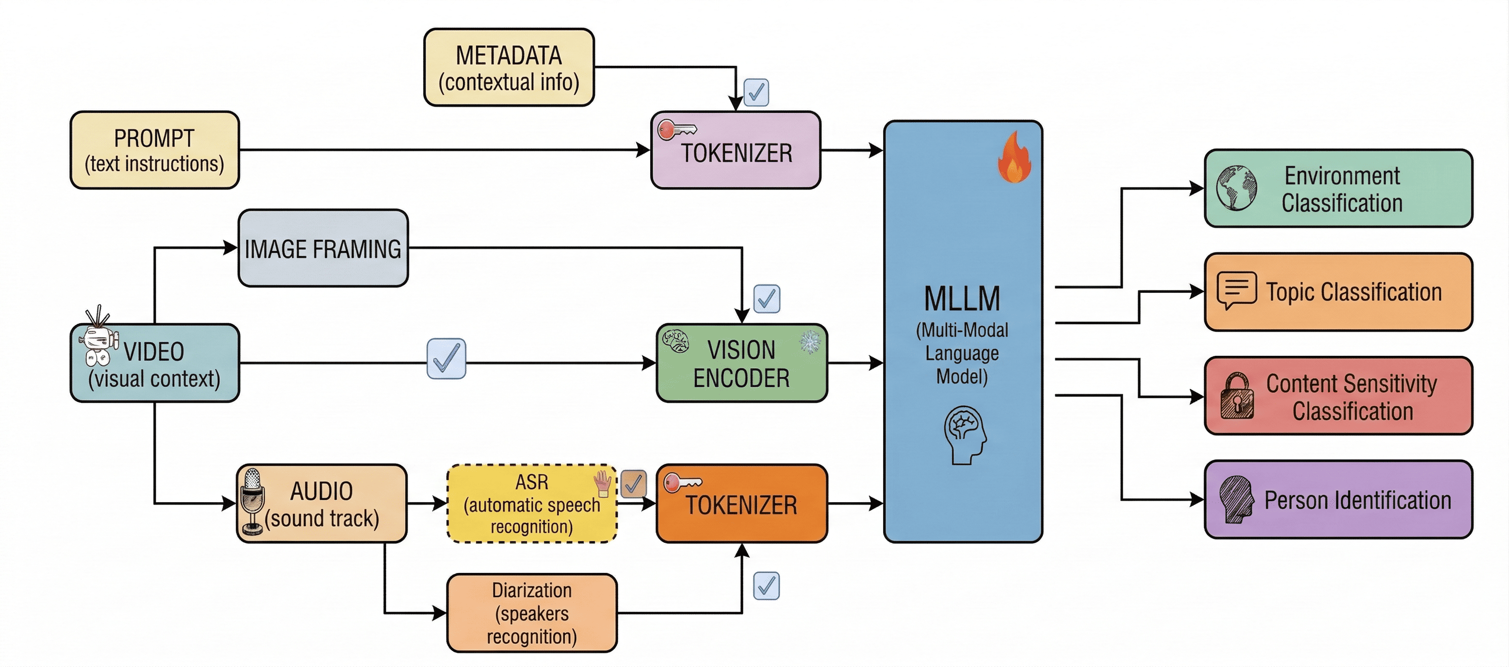
Pipeline. The production system (Figure 1) shares a single architecture across all configurations. An audio–textual branch transcribes speech with Faster-Whisper, optionally adds speaker diarization via
pyannote, and optionally appends episode-level metadata (program title, broadcast date, genre, and expected guests). A visual branch is instantiated either as sampled static frames or as the native video clip. The branches feed an MLLM that
returns, per minute, a structured JSON record over four tasks. Activating subsets of the optional components yields a grid of input configurations, ranging from visual-only to visual\(+\)ASR\(+\)diarization\(+\)metadata, that lets us isolate the contribution of each textual source. The exact configuration set differs slightly between the two visual branches and is enumerated in
Appendix 10: notably, the video branch includes a visual\(+\)metadata configuration without ASR—the one ultimately selected for deployment (Section 5).
Tasks and taxonomy. Each minute is annotated along four dimensions, inspired by the IAB Content Taxonomy [22] and adapted to Italian prime-time television. Topic classification assigns one label from a 28-label taxonomy (14 macro-areas). Environment classification assigns one of 22 setting labels. Visual named-entity recognition lists individuals visually present (empty if none). Sensitive-content detection flags material across six categories drawn from content-moderation and broadcast regulatory frameworks. The taxonomy was refined iteratively with broadcast domain experts; the full label set is in Appendix 7.
Deployment setting. The selected configuration (Gemini-3-Pro with video and episode-level metadata) is deployed on 14 full episodes of a single fixed-slot weekly program, annotating 3,104 minutes at one-minute granularity (advertising excluded). Audience metrics are supplied by an Italian media company in aggregated, normalized form; no personally identifiable information is accessed.
4 Choosing the Production Configuration↩︎
Diagnostic benchmark. To select a configuration under realistic constraints, we built a diagnostic test set of 100 one-minute clips from Italian broadcast programs aired in 2025, stratified across four editorial macro-categories—current-affairs talk shows, investigative, cultural, and lifestyle programs—with 25 clips sampled per category (one per episode) to balance editorial conditions by design; program identities are anonymized. Clips are extracted without enforcing scene boundaries and may span multiple shots, speaker turns, and topic transitions, reflecting operational conditions rather than curated single-topic segments. Two annotators with TV-content experience labeled all clips; inter-annotator agreement (Cohen’s \(\kappa\)) was 0.70 (topic), 0.67 (environment), and 0.67 (entities); sensitive content reached \(\kappa{=}1.0\), interpreted cautiously given only 12 positive clips. Disagreements were resolved by consensus. We evaluate nine MLLMs spanning proprietary and open-weight families—Gemini-3-Pro, GPT-5-mini, Llama-4-Maverick, Qwen2.5-VL-72B, Qwen3-VL (235B/30B/8B), Gemma-3-27B, and Ministral-14B—in the frame setting, and the six models supporting native video input (Gemini-3-Pro, Qwen3-Omni, Qwen3-VL-235B, Qwen3-VL-30B, Molmo-2-8B, and Seed-1.6) for the cross-pipeline comparison, in a zero-shot setting with a single prompt template that includes the full taxonomy (Appendix 8). Predictions outside the label set are scored as incorrect. Input token counts from model APIs are reported as an explicit proxy for cost.
Component choices. Preliminary studies fixed the visual and ASR components. Accuracy plateaus beyond 12 frames across all models, and shot-based sampling offers no advantage on this material; uniform sampling at 0.2 fps (12 frames) cuts token use by \({\sim}40\%\) relative to an 18-frame budget at comparable accuracy. Across the ASR systems compared, Faster-Whisper Medium offers competitive downstream quality without the latency overhead of larger variants, making it suitable for cost-efficient large-scale inference. This fixes the ASR component for the benchmark configurations that include it; the configuration ultimately deployed omits ASR altogether (Section 5).
What drives quality. Task quality is shaped by the interaction of input modality and model capacity, not by raw visual richness (Table 2). The frame pipeline’s
only/asr/asr_meta configurations let us isolate each textual source within a fixed model: only\(\rightarrow\)asr isolates the ASR increment,
asr\(\rightarrow\)asr_meta the metadata increment. For topic, the isolated ASR increment is large and consistent (\(+0.14\) to \(+0.21\) accuracy for Gemini-3-Pro, Llama-4-Maverick, and the Qwen models), while the subsequent metadata increment is near zero: speech-derived text is the driver and diarization adds no systematic benefit. For visual
NER—the most demanding task—the pattern reverses: the ASR increment is negligible whereas the isolated metadata increment dominates (precision \(0.08\rightarrow0.52\) for Qwen3-VL-235B and Qwen3-VL-30B, \(0.42\rightarrow0.60\) for Gemini-3-Pro), though enrichment is not uniformly safe—diarization noise degrades identity resolution for several models, and smaller models hallucinate identities without textual grounding.
Environment is primarily perceptual; whether native video helps is model-dependent (Table 1), with gains concentrated in motion-dependent or spatially ambiguous scenes. Sensitive-content detection is
dominated by false-positive control: transcripts can contextualize ambiguous scenes but also trigger spurious activations via lexical shortcuts, especially in smaller models; with only 12 positive clips, its metrics are diagnostic and do not drive
configuration selection.
Video is not universally better (controlled comparison). Critically, native video input does not systematically outperform sampled frames. To isolate the visual representation from confounds of model capacity and textual input, we compare the two pipelines within each of the three architectures common to both (Gemini-3-Pro, Qwen3-VL-235B, Qwen3-VL-30B) at matched input compositions (Table 1). Holding model and textual inputs fixed, the video\(-\)frame accuracy gap is small and, in most cells, not statistically distinguishable from zero: of the eighteen matched comparisons, twelve have a 95% bootstrap confidence interval (paired over clips) that spans zero. For topic, video helps only when no transcript is present (Gemini-3-Pro \(+0.12\), CI \([{+}0.05,{+}0.20]\); Qwen3-VL-30B \(+0.14\), CI \([{+}0.05,{+}0.24]\)) and the gain becomes indistinguishable from zero once ASR is added. For environment, the significant effects are model-specific and of opposite sign: video helps Qwen3-VL-30B substantially (\(+0.36\), CI \([{+}0.23,{+}0.48]\)) but hurts the larger Gemini-3-Pro (\(-0.10\), CI \([{-}0.19,{-}0.01]\)). The residual token gap between the two encodings is intrinsic to the representation and is reported, not equalized (Appendix 10). This within-model evidence—bounded to three architectures and a 100-clip set—substantiates the headline result under controlled conditions: the video benefit does not track model size and is confined to a few model–task cells, while degradation under extended multimodal context appears among the smaller video-only models in the full results (Appendix 10). Combined with the token-cost accounting, this argues against adopting video ingestion as a default. We select Gemini-3-Pro with video plus metadata for deployment: it is not Pareto-dominant (accepting a small environment loss, 0.73 vs. for frames\(+\)ASR\(+\)metadata) but gives the best topic accuracy (0.83) at roughly half the token cost. It omits ASR—for the highest-capacity model, metadata already supplies enough textual context (topic 0.83 vs. with ASR)—which in a corporate setting also drops a transcription stage and its hardware, lowering latency and improving portability.
| Model | Input | \(\Delta\)Topic | 95% CI | \(\Delta\)Env | 95% CI |
|---|---|---|---|---|---|
| Gemini-3-Pro | only | \(\mathbf{+0.12}\) | \([{+}0.05,{+}0.20]\) | \(-0.04\) | \([{-}0.13,{+}0.05]\) |
| asr+meta | \(+0.01\) | \([{-}0.04,{+}0.06]\) | \(\mathbf{-0.10}\) | \([{-}0.19,{-}0.01]\) | |
| +diar | \(+0.01\) | \([{-}0.03,{+}0.05]\) | \(+0.01\) | \([{-}0.08,{+}0.10]\) | |
| Qwen3-VL-235B | only | \(+0.04\) | \([{-}0.04,{+}0.12]\) | \(+0.06\) | \([{-}0.02,{+}0.14]\) |
| asr+meta | \(+0.01\) | \([{-}0.07,{+}0.10]\) | \(+0.04\) | \([{-}0.05,{+}0.13]\) | |
| +diar | \(+0.05\) | \([{-}0.06,{+}0.15]\) | \(+0.03\) | \([{-}0.07,{+}0.13]\) | |
| Qwen3-VL-30B | only | \(\mathbf{+0.14}\) | \([{+}0.05,{+}0.24]\) | \(\mathbf{+0.19}\) | \([{+}0.09,{+}0.30]\) |
| asr+meta | \(+0.05\) | \([{-}0.04,{+}0.14]\) | \(\mathbf{+0.36}\) | \([{+}0.23,{+}0.48]\) | |
| +diar | \(+0.07\) | \([{-}0.02,{+}0.16]\) | \(\mathbf{+0.20}\) | \([{+}0.09,{+}0.32]\) |
6pt
Error patterns. Manual inspection reveals failure modes the aggregate metrics obscure. Topic errors are systematic collapses between adjacent labels (international \(\rightarrow\) domestic politics), driven by shared lexical fields in the transcript; environment errors cluster within perceptually similar settings (home apartment vs.corporate office), while distinctive studio layouts stay stable. Sensitive-content errors stem from threshold instability—under weak visual evidence, lexical triggers induce spurious activations, turning text into a liability—and entity-recognition failures concentrate in smaller models and in clips lacking textual anchors, where models hallucinate identities. Model capacity moderates these effects but does not remove the underlying bottlenecks.
| Task | Driver | Video | Failure mode |
|---|---|---|---|
| Topic | Speech | Low | Semantic overlap |
| Environment | Visual | Var. | Spatial ambiguity |
| Sensitive | Visual | n/a | Spurious activation |
| Entities | Metadata | Low | Identity halluc. |
4pt
5 Deployment and Audience Analytics↩︎
Production cost and throughput. Table 3 summarizes deployment economics. The selected configuration consumes \({\sim}6.4\)K input tokens per annotated minute and emits only four structured fields, so annotating the full corpus costs \({\approx}\$40\) at list pricing1 (\({\approx}\$20\) via the Batch API)—under a cent and a half per minute. Median latency (\({\sim}31\) s/minute, real-time factor \({\approx}0.5\)) means a single request stream keeps pace with broadcast; annotation is offline and trivially parallelizable. Notably, native video\(+\)metadata is also more token-economical than the frame configuration (\({\sim}6.4\)K vs \({\sim}14.6\)K tokens/minute): the model encodes native video at a low fixed token rate per sampled second, whereas twelve full-resolution stills each consume a large token block. The production choice is therefore simultaneously the higher-quality and the cheaper one.
| Production metric | Value |
|---|---|
| Input tokens / annotated minute | \({\sim}6{,}443\) |
| Total input tokens (3,104 min) | \({\sim}20.0\)M |
| Output tokens / call | 4 fields (negl.) |
| API latency / minute | \({\sim}31\) s |
| Real-time factor | \({\approx}0.52\) |
| Est.cost, list ($2 / 1M in) | \({\approx}\$40\) |
| per annotated minute | \({\approx}\$0.013\) |
| per hour of broadcast | \({\approx}\$0.8\) |
| Est.cost, Batch API (\(-50\%\)) | \({\approx}\$20\) |
6pt
Human-cost comparison. The media partner’s manual workflow for the same deliverable is estimated at roughly two analyst-hours per episode (one to annotate content, one to ingest audience data and produce the analysis): \({\approx}28\) hours per 14-episode cycle, or \({\approx}\,\)€840 at an illustrative €30/h, against \({\approx}\$40\) of compute plus the residual human time to confirm sensitive-content flags—an order-of-magnitude gap that widens with scale, since manual effort grows linearly with airtime while per-minute annotation cost is fixed. The manual figure reflects a coarse operational pass, not the research-grade annotation used for the benchmark, and only bounds the saving.
Content characterization. On the 3,104 deployed minutes, editorial structure is highly concentrated: domestic politics (40.8%) and international politics (21.7%) account for over 60% of airtime, followed by economy and finance (11.7%), humor and satire (9.2%), and crime and justice (6.0%); remaining topics form a long tail. The NER module identifies 143 unique guests (hosts excluded) over 3,717 minute-level occurrences. Participation is structurally asymmetric: male guests account for 81.1% of occurrences (89 individuals, 33.9 appearances each on average) versus 700 occurrences across 54 female guests (13.0 each), and 80.2% of minutes feature exclusively male guests—a pattern replicated across episodes. Since visual NER operates at F1\(\,{\approx}\,\)0.60 at deployment, these absolute participation figures should be read as approximate estimates rather than exact counts; the asymmetry itself, however, is large and directionally robust to this error rate, illustrating the kind of large-scale content audit the pipeline makes feasible.
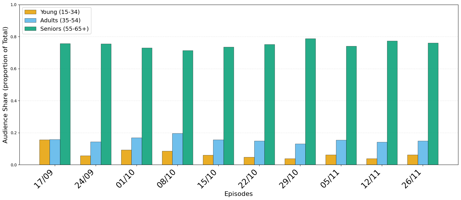
Baseline audience composition. Figure 2 reports normalized AMR per episode by age cohort (Young 15–34, Adults 35–54, Seniors 55+). The senior segment is the largest and most stable component; younger viewers show markedly higher inter-episode variability, indicating that episode-level fluctuations are driven mainly by changes in younger participation rather than the senior base.
Topic-level sensitivity and divergence. Audience values are normalized intra-episode via per-cohort \(z\)-scores (Appendix 9), so positive values indicate above-average engagement controlling for episode popularity and seasonality. Among the ten topics with the largest inter-cohort \(z\)-score gap, art and literature is positive for Young viewers yet negative for Adults and Seniors—the clearest case of cohort-selective engagement. A gradient pattern characterizes music, health and wellness, and sports–football: negative across cohorts, with the decline steepening with age. Family and relationships and environment and climate are associated with disengagement across all groups, while food and cooking and sports–other act as shared attractors that differ in amplitude rather than direction.
Interpretation. High-frequency structural topics sustain a stable engagement backbone, while low-frequency episodic segments generate localized deviations that differentially affect age cohorts—a shift from static aggregate measurement toward dynamic audience-sensitivity analysis of direct value for editorial planning. We present this integration as an illustrative downstream use enabled by the annotations rather than a standalone analytical contribution; all reported patterns are observational and no causal claims are made.
6 Lessons Learned and Conclusion↩︎
Speech and text beat video for the language-oriented tasks. Video pipelines do not systematically outperform frame configurations: under a controlled within-model comparison, most matched gaps are statistical ties and the few significant effects are model-specific and of opposite sign, not a function of model size (degradation under extended multimodal context shows up mainly in the smaller video-only models). Video ingestion should be a conditional design choice, validated per task and per model before its cost is accepted.
Metadata is the cheapest high-impact lever. Isolating each textual increment, episode-level metadata was the dominant driver for entity resolution—outweighing transcription quality there at negligible token cost—whereas speech transcripts, not metadata, drove topic. In a deployment, cheap structured side information is often more valuable than a heavier perceptual modality for the tasks it targets.
Taxonomy design is a first-order engineering decision. Recurring errors—semantic collapse between adjacent topics, perceptual confusion between similar environments—were attributable to label structure, not model capacity: overlapping or underspecified categories introduce systematic ambiguity that no extra modality resolves. The taxonomy should be a maintained engineering artifact, not a fixed schema.
Automated annotation enables scale but needs error-aware use. Annotating at inference speed makes longitudinal audits and cross-program comparisons feasible, but systematic label biases (environment misclassification, topic conflation) propagate downstream. We add two safeguards: the lowest-precision task (sensitive-content detection) is human-confirmed before any downstream use rather than driving autonomous decisions, and a rolling sample of deployed minutes is periodically re-annotated to monitor drift, seeded by the diagnostic benchmark. Studies built on automated annotations should carry reliability proxies, and findings from borderline categories should be read as indicative.
Taken together, these lessons show that deployed multimodal annotation should match each task to the cheapest reliable signal rather than defaulting to the richest input. In our broadcast setting, speech supported topic interpretation, metadata stabilized entity resolution, and vision remained necessary for perceptual labels. Under these safeguards, such annotations can support scalable audience analysis and content audits without treating automated labels as ground truth.
Limitations↩︎
The diagnostic benchmark (100 clips) limits statistical robustness and generalizability and should be read as diagnostic rather than as a large-scale corpus. The cross-pipeline comparison is controlled within the three architectures common to both pipelines and at matched textual inputs, but video and frame encodings cannot be equalized in token count; the residual token gap is an intrinsic property of the representation rather than a nuisance variable we control away. Bootstrap confidence intervals are reported for the controlled cross-pipeline comparison; the remaining per-model tables report point estimates only. Although the clips are stratified by editorial macro-category, they remain internally heterogeneous (multiple shots, speakers, and topic transitions per minute), so per-signal effects are reported descriptively and may partly reflect clip composition. The taxonomies are tailored to a specific broadcast format and may require adaptation elsewhere. The evaluation is monolingual (Italian) and centered on a single program type, leaving multilingual content and other genres untested. All experiments use zero-shot prompting of general-purpose models, without task-specific fine-tuning. The audience analyses are purely observational: intra-episode per-cohort \(z\)-score normalization removes episode-level popularity and seasonality, but the analysis is not benchmarked against simpler scheduling baselines, reported associations between content and engagement do not establish causal relationships, and they may be confounded by concurrent programming. Finally, downstream analyses inherit the annotation error profile of the pipeline, which is only partially characterized at this scale.
Ethical Considerations↩︎
Audience data were provided by the media partner in aggregated and normalized form, disaggregated only by coarse age cohorts; no personally identifiable information was accessed or stored. The system performs sensitive-content detection and visual entity recognition over public broadcast material; we report these capabilities for analytical and editorial-planning purposes and caution against punitive or surveillance uses. Automated annotation can encode and amplify bias: the observed gender asymmetry in guest participation is a property of the broadcast content, but pipeline errors could distort such measurements, so demographic findings should be validated before informing decisions. Program and company identities are anonymized, and proprietary data are not released. We follow the ACL Code of Ethics.
7 Complete Annotation Taxonomy↩︎
Table 4 lists the full label sets for topic, environment, and sensitive-content annotation.
| Topic | Environment | Sensitive |
|---|---|---|
| Domestic politics | Studio – Single host | Violence |
| International politics | Studio – 1-to-1 interview | Blood |
| Crime and justice | Studio – Guest panel | War / armed conflicts |
| Environment and climate | Studio – Remote split screen | Organized crime |
| Society and social phenomena | Studio – Video segment | Humanitarian crises |
| Family and relationships | Home – Apartment | Self-harm / suicide |
| Cinema, TV and entertainment | Home – Kitchen | |
| Music | Corporate office | |
| Humor and satire | Commercial/public venue | |
| Art and literature | Spa/wellness center | |
| History and archaeology | Vehicle/transport | |
| Religion and spirituality | Generic urban outdoor | |
| Science and technology | Nature – Outdoors | |
| Education and training | Nature – Mountain | |
| Food and cooking | Identified tourist site | |
| Fashion and beauty | ||
| Travel and tourism | ||
| Health and wellness | ||
| Motors and vehicles | ||
| Sports – Football | ||
| Sports – Other |
8 Prompt Strategies↩︎
Both pipelines share the output schema and hard constraints: select exactly one label for topic and environment, at most one sensitive-content flag, include a guest name only if the person is visually recognized or explicitly named, and return JSON only. Configurations differ in which sources are provided and in their relative authority. When metadata is added, it is explicitly subordinated to visual evidence (used only to confirm or correct visually recognized identities, never to assume presence). When ASR is added, a three-level hierarchy is established: video is primary for visual elements, ASR for spoken content, and metadata acts as a correction layer for proper nouns and context.
9 Audience Normalization↩︎
Topic-level audience sensitivity (Section 5) is computed on per-cohort, intra-episode \(z\)-scores. Let \(c\) index the age cohort, \(e\) the episode, and \(t\) the topic. Let \(x_{c,e,t}\) be the mean normalized AMR of cohort \(c\) over the minutes labeled with topic \(t\) in episode \(e\), and let \(\mu_{c,e}\) and \(\sigma_{c,e}\) be the mean and standard deviation of cohort \(c\)’s per-minute normalized AMR within episode \(e\). The \(z\)-score is \[z_{c,e,t} \;=\; \frac{x_{c,e,t}-\mu_{c,e}}{\sigma_{c,e}} .\] Normalizing within each episode and cohort removes differences in baseline popularity and seasonality, so positive (negative) values denote above-average (below-average) engagement of a cohort with a topic relative to its own episode-level mean. The inter-cohort gap discussed in Section 5 is the spread of \(z_{c,e,t}\) across cohorts, averaged over episodes.
10 Full Per-Model Results↩︎
Complete per-model, per-configuration results for all four tasks. We report Accuracy, Precision, Recall, and F1, together with input tokens (Tok) and average API latency in milliseconds (Lat). The video pipeline covers the six models supporting native video; the frame pipeline covers all nine models. Tables 1–4 report the video pipeline and Tables 5–8 the frame pipeline.
| Model | Input | Acc | Prec | Rec | F1 | Tok | Lat |
|---|---|---|---|---|---|---|---|
| Table – continued | |||||||
| Model | Input | Acc | Prec | Rec | F1 | Tok | Lat |
| continued on next page | |||||||
| gemini-3-pro | asr_diar_meta | 0.74 | 0.79 | 0.74 | 0.75 | 6856 | 31932 |
| gemini-3-pro | asr_meta | 0.66 | 0.76 | 0.66 | 0.68 | 6732 | 29595 |
| gemini-3-pro | meta | 0.73 | 0.79 | 0.73 | 0.75 | 6443 | 31008 |
| gemini-3-pro | only | 0.66 | 0.73 | 0.66 | 0.68 | 6224 | 35729 |
| molmo-2-8b | asr_diar_meta | 0.33 | 0.42 | 0.33 | 0.29 | 12197 | 22064 |
| molmo-2-8b | asr_meta | 0.14 | 0.06 | 0.14 | 0.06 | 11846 | 26757 |
| molmo-2-8b | meta | 0.26 | 0.68 | 0.26 | 0.24 | 11608 | 24596 |
| molmo-2-8b | only | 0.18 | 0.60 | 0.18 | 0.14 | 11361 | 21761 |
| qwen3-omni | asr_diar_meta | 0.54 | 0.49 | 0.54 | 0.49 | 15346 | 9525 |
| qwen3-omni | asr_meta | 0.56 | 0.56 | 0.56 | 0.53 | 15207 | 9735 |
| qwen3-omni | meta | 0.55 | 0.63 | 0.55 | 0.54 | 14861 | 9879 |
| qwen3-omni | only | 0.55 | 0.55 | 0.55 | 0.53 | 14615 | 9913 |
| qwen3-235b | asr_diar_meta | 0.65 | 0.65 | 0.65 | 0.62 | 14614 | 7178 |
| qwen3-235b | asr_meta | 0.71 | 0.73 | 0.71 | 0.71 | 14475 | 7237 |
| qwen3-235b | meta | 0.70 | 0.72 | 0.70 | 0.69 | 14129 | 7091 |
| qwen3-235b | only | 0.71 | 0.74 | 0.71 | 0.71 | 13884 | 9023 |
| qwen3-30b | asr_diar_meta | 0.62 | 0.58 | 0.62 | 0.57 | 14614 | 22218 |
| qwen3-30b | asr_meta | 0.66 | 0.60 | 0.66 | 0.62 | 14475 | 13720 |
| qwen3-30b | meta | 0.71 | 0.77 | 0.71 | 0.69 | 14130 | 20742 |
| qwen3-30b | only | 0.70 | 0.78 | 0.70 | 0.69 | 13884 | 18405 |
| seed-1.6 | asr_diar_meta | 0.42 | 0.48 | 0.42 | 0.40 | 19506 | 40369 |
| seed-1.6 | asr_meta | 0.54 | 0.65 | 0.54 | 0.56 | 19361 | 34226 |
| seed-1.6 | meta | 0.61 | 0.64 | 0.61 | 0.61 | 19036 | 33848 |
| seed-1.6 | only | 0.58 | 0.56 | 0.58 | 0.56 | 18799 | 57734 |
| Model | Input | Acc | Prec | Rec | F1 | Tok | Lat |
|---|---|---|---|---|---|---|---|
| Table – continued | |||||||
| Model | Input | Acc | Prec | Rec | F1 | Tok | Lat |
| continued on next page | |||||||
| gemini-3-pro | asr_diar_meta | 0.81 | 0.82 | 0.81 | 0.80 | 6856 | 31932 |
| gemini-3-pro | asr_meta | 0.80 | 0.82 | 0.80 | 0.79 | 6732 | 29595 |
| gemini-3-pro | meta | 0.83 | 0.82 | 0.83 | 0.81 | 6443 | 31008 |
| gemini-3-pro | only | 0.79 | 0.79 | 0.79 | 0.77 | 6224 | 35729 |
| molmo-2-8b | asr_diar_meta | 0.53 | 0.68 | 0.53 | 0.53 | 12197 | 22064 |
| molmo-2-8b | asr_meta | 0.60 | 0.73 | 0.60 | 0.62 | 11846 | 26757 |
| molmo-2-8b | meta | 0.50 | 0.67 | 0.50 | 0.52 | 11608 | 24596 |
| molmo-2-8b | only | 0.34 | 0.62 | 0.34 | 0.36 | 11361 | 21761 |
| qwen3-omni | asr_diar_meta | 0.76 | 0.75 | 0.76 | 0.74 | 15346 | 9525 |
| qwen3-omni | asr_meta | 0.77 | 0.79 | 0.77 | 0.77 | 15207 | 9735 |
| qwen3-omni | meta | 0.78 | 0.80 | 0.78 | 0.77 | 14861 | 9879 |
| qwen3-omni | only | 0.78 | 0.82 | 0.78 | 0.78 | 14615 | 9913 |
| qwen3-235b | asr_diar_meta | 0.69 | 0.74 | 0.69 | 0.69 | 14614 | 7178 |
| qwen3-235b | asr_meta | 0.70 | 0.73 | 0.70 | 0.69 | 14475 | 7237 |
| qwen3-235b | meta | 0.63 | 0.70 | 0.63 | 0.64 | 14129 | 7091 |
| qwen3-235b | only | 0.55 | 0.68 | 0.55 | 0.57 | 13884 | 9023 |
| qwen3-30b | asr_diar_meta | 0.69 | 0.77 | 0.69 | 0.70 | 14614 | 22218 |
| qwen3-30b | asr_meta | 0.71 | 0.78 | 0.71 | 0.72 | 14475 | 13720 |
| qwen3-30b | meta | 0.65 | 0.69 | 0.65 | 0.65 | 14130 | 20742 |
| qwen3-30b | only | 0.60 | 0.68 | 0.60 | 0.60 | 13884 | 18405 |
| seed-1.6 | asr_diar_meta | 0.75 | 0.79 | 0.75 | 0.76 | 19506 | 40369 |
| seed-1.6 | asr_meta | 0.71 | 0.70 | 0.71 | 0.70 | 19361 | 34226 |
| seed-1.6 | meta | 0.60 | 0.73 | 0.60 | 0.63 | 19036 | 33848 |
| seed-1.6 | only | 0.45 | 0.68 | 0.45 | 0.50 | 18799 | 57734 |
| Model | Input | Acc | Prec | Rec | F1 | Tok | Lat |
|---|---|---|---|---|---|---|---|
| Table – continued | |||||||
| Model | Input | Acc | Prec | Rec | F1 | Tok | Lat |
| continued on next page | |||||||
| gemini-3-pro | asr_diar_meta | 0.89 | 0.50 | 0.82 | 0.62 | 6856 | 31932 |
| gemini-3-pro | asr_meta | 0.85 | 0.41 | 0.82 | 0.55 | 6732 | 29595 |
| gemini-3-pro | meta | 0.88 | 0.47 | 0.64 | 0.54 | 6443 | 31008 |
| gemini-3-pro | only | 0.88 | 0.47 | 0.73 | 0.57 | 6224 | 35729 |
| molmo-2-8b | asr_diar_meta | 0.90 | 0.43 | 0.33 | 0.38 | 12197 | 22064 |
| molmo-2-8b | asr_meta | 0.84 | 0.27 | 0.44 | 0.33 | 11846 | 26757 |
| molmo-2-8b | meta | 0.82 | 0.24 | 0.44 | 0.31 | 11608 | 24596 |
| molmo-2-8b | only | 0.88 | 0.25 | 0.10 | 0.14 | 11361 | 21761 |
| qwen3-omni | asr_diar_meta | 0.69 | 0.22 | 0.89 | 0.35 | 15346 | 9525 |
| qwen3-omni | asr_meta | 0.68 | 0.21 | 0.89 | 0.34 | 15207 | 9735 |
| qwen3-omni | meta | 0.73 | 0.24 | 0.89 | 0.38 | 14861 | 9879 |
| qwen3-omni | only | 0.91 | 0.57 | 0.40 | 0.47 | 14615 | 9913 |
| qwen3-235b | asr_diar_meta | 0.77 | 0.23 | 0.67 | 0.34 | 14614 | 7178 |
| qwen3-235b | asr_meta | 0.74 | 0.19 | 0.63 | 0.29 | 14475 | 7237 |
| qwen3-235b | meta | 0.79 | 0.23 | 0.56 | 0.32 | 14129 | 7091 |
| qwen3-235b | only | 0.84 | 0.29 | 0.56 | 0.38 | 13884 | 9023 |
| qwen3-30b | asr_diar_meta | 0.77 | 0.25 | 0.78 | 0.38 | 14614 | 22218 |
| qwen3-30b | asr_meta | 0.78 | 0.29 | 0.80 | 0.42 | 14475 | 13720 |
| qwen3-30b | meta | 0.73 | 0.18 | 0.56 | 0.27 | 14130 | 20742 |
| qwen3-30b | only | 0.71 | 0.17 | 0.63 | 0.26 | 13884 | 18405 |
| seed-1.6 | asr_diar_meta | 0.88 | 0.33 | 0.09 | 0.14 | 19506 | 40369 |
| seed-1.6 | asr_meta | 0.89 | 0.50 | 0.36 | 0.42 | 19361 | 34226 |
| seed-1.6 | meta | 0.87 | 0.00 | 0.00 | – | 19036 | 33848 |
| seed-1.6 | only | 0.89 | 1.00 | 0.08 | 0.15 | 18799 | 57734 |
| Model | Input | Acc | Prec | Rec | F1 | Tok | Lat |
|---|---|---|---|---|---|---|---|
| Table – continued | |||||||
| Model | Input | Acc | Prec | Rec | F1 | Tok | Lat |
| continued on next page | |||||||
| gemini-3-pro | asr_diar_meta | 0.60 | 0.62 | 0.60 | 0.61 | 6856 | 31932 |
| gemini-3-pro | asr_meta | 0.50 | 0.56 | 0.50 | 0.52 | 6732 | 29595 |
| gemini-3-pro | meta | 0.60 | 0.63 | 0.60 | 0.60 | 6443 | 31008 |
| gemini-3-pro | only | 0.50 | 0.54 | 0.50 | 0.50 | 6224 | 35729 |
| molmo-2-8b | asr_diar_meta | 0.14 | 0.18 | 0.14 | 0.10 | 12197 | 22064 |
| molmo-2-8b | asr_meta | 0.13 | 0.11 | 0.13 | 0.07 | 11846 | 26757 |
| molmo-2-8b | meta | 0.10 | 0.01 | 0.10 | 0.02 | 11608 | 24596 |
| molmo-2-8b | only | 0.10 | 0.01 | 0.10 | 0.02 | 11361 | 21761 |
| qwen3-omni | asr_diar_meta | 0.10 | 0.01 | 0.10 | 0.02 | 15346 | 9525 |
| qwen3-omni | asr_meta | 0.10 | 0.01 | 0.10 | 0.02 | 15207 | 9735 |
| qwen3-omni | meta | 0.10 | 0.01 | 0.10 | 0.02 | 14861 | 9879 |
| qwen3-omni | only | 0.10 | 0.01 | 0.10 | 0.02 | 14615 | 9913 |
| qwen3-235b | asr_diar_meta | 0.13 | 0.14 | 0.13 | 0.06 | 14614 | 7178 |
| qwen3-235b | asr_meta | 0.18 | 0.17 | 0.18 | 0.12 | 14475 | 7237 |
| qwen3-235b | meta | 0.13 | 0.09 | 0.13 | 0.06 | 14129 | 7091 |
| qwen3-235b | only | 0.15 | 0.06 | 0.15 | 0.07 | 13884 | 9023 |
| qwen3-30b | asr_diar_meta | 0.10 | 0.01 | 0.10 | 0.02 | 14614 | 22218 |
| qwen3-30b | asr_meta | 0.10 | 0.01 | 0.10 | 0.02 | 14475 | 13720 |
| qwen3-30b | meta | 0.10 | 0.01 | 0.10 | 0.02 | 14130 | 20742 |
| qwen3-30b | only | 0.18 | 0.10 | 0.18 | 0.12 | 13884 | 18405 |
| seed-1.6 | asr_diar_meta | 0.42 | 0.40 | 0.42 | 0.38 | 19506 | 40369 |
| seed-1.6 | asr_meta | 0.39 | 0.38 | 0.39 | 0.37 | 19361 | 34226 |
| seed-1.6 | meta | 0.31 | 0.31 | 0.31 | 0.26 | 19036 | 33848 |
| seed-1.6 | only | 0.10 | 0.01 | 0.10 | 0.02 | 18799 | 57734 |
| Model | Input | Acc | Prec | Rec | F1 | Tok | Lat |
|---|---|---|---|---|---|---|---|
| Table – continued | |||||||
| Model | Input | Acc | Prec | Rec | F1 | Tok | Lat |
| continued on next page | |||||||
| gemini-3-pro | asr | 0.68 | 0.72 | 0.68 | 0.68 | 14294 | 35028 |
| gemini-3-pro | asr_diar | 0.72 | 0.77 | 0.72 | 0.72 | 14456 | 33811 |
| gemini-3-pro | asr_diar_meta | 0.73 | 0.79 | 0.73 | 0.74 | 14666 | 34378 |
| gemini-3-pro | asr_meta | 0.76 | 0.81 | 0.76 | 0.77 | 14572 | 32011 |
| gemini-3-pro | only | 0.70 | 0.75 | 0.70 | 0.71 | 13996 | 34865 |
| gemma-3-27b | asr | 0.46 | 0.51 | 0.46 | 0.43 | 4212 | 25520 |
| gemma-3-27b | asr_diar | 0.47 | 0.29 | 0.47 | 0.36 | 4376 | 28385 |
| gemma-3-27b | asr_diar_meta | 0.44 | 0.30 | 0.44 | 0.34 | 4586 | 8738 |
| gemma-3-27b | asr_meta | 0.37 | 0.47 | 0.37 | 0.34 | 4491 | 29150 |
| gemma-3-27b | only | 0.49 | 0.45 | 0.49 | 0.45 | 3917 | 8167 |
| gpt-5-mini | asr | 0.55 | 0.50 | 0.55 | 0.52 | 4551 | 37385 |
| gpt-5-mini | asr_diar | 0.27 | 0.51 | 0.27 | 0.34 | 4705 | 55330 |
| gpt-5-mini | asr_diar_meta | 0.56 | 0.62 | 0.56 | 0.58 | 4945 | 28378 |
| gpt-5-mini | asr_meta | 0.46 | 0.72 | 0.46 | 0.54 | 4849 | 45219 |
| gpt-5-mini | only | 0.59 | 0.64 | 0.59 | 0.59 | 4234 | 15836 |
| llama-4-mav | asr | 0.57 | 0.64 | 0.57 | 0.59 | 9753 | 20462 |
| llama-4-mav | asr_diar | 0.58 | 0.56 | 0.58 | 0.54 | 9906 | 24420 |
| llama-4-mav | asr_diar_meta | 0.60 | 0.68 | 0.60 | 0.57 | 10135 | 8195 |
| llama-4-mav | asr_meta | 0.54 | 0.62 | 0.54 | 0.56 | 10056 | 19666 |
| llama-4-mav | only | 0.55 | 0.60 | 0.55 | 0.56 | 9461 | 4710 |
| ministral-14b | asr | 0.28 | 0.30 | 0.28 | 0.25 | 5441 | 19854 |
| ministral-14b | asr_diar | 0.21 | 0.37 | 0.21 | 0.15 | 5620 | 21727 |
| ministral-14b | asr_diar_meta | 0.20 | 0.35 | 0.20 | 0.22 | 5868 | 10670 |
| ministral-14b | asr_meta | 0.08 | 0.22 | 0.08 | 0.10 | 5742 | 26039 |
| ministral-14b | only | 0.25 | 0.27 | 0.25 | 0.22 | 5124 | 7118 |
| qwen2.5-72b | asr | 0.60 | 0.62 | 0.60 | 0.58 | 4821 | 19667 |
| qwen2.5-72b | asr_diar | 0.53 | 0.47 | 0.53 | 0.46 | 4983 | 23429 |
| qwen2.5-72b | asr_diar_meta | 0.59 | 0.47 | 0.59 | 0.50 | 5241 | 6494 |
| qwen2.5-72b | asr_meta | 0.56 | 0.51 | 0.56 | 0.52 | 5150 | 19650 |
| qwen2.5-72b | only | 0.63 | 0.67 | 0.63 | 0.62 | 4460 | 7222 |
| qwen3-235b | asr | 0.65 | 0.63 | 0.65 | 0.62 | 3863 | 21662 |
| qwen3-235b | asr_diar | 0.57 | 0.58 | 0.57 | 0.54 | 4024 | 21450 |
| qwen3-235b | asr_diar_meta | 0.62 | 0.58 | 0.62 | 0.57 | 4283 | 6062 |
| qwen3-235b | asr_meta | 0.67 | 0.70 | 0.67 | 0.67 | 4192 | 20654 |
| qwen3-235b | only | 0.65 | 0.62 | 0.65 | 0.63 | 3501 | 3617 |
| qwen3-30b | asr | 0.56 | 0.55 | 0.56 | 0.53 | 3863 | 19758 |
| qwen3-30b | asr_diar | 0.44 | 0.36 | 0.44 | 0.35 | 4024 | 16779 |
| qwen3-30b | asr_diar_meta | 0.41 | 0.41 | 0.41 | 0.34 | 4283 | 5855 |
| qwen3-30b | asr_meta | 0.30 | 0.49 | 0.30 | 0.28 | 4192 | 16132 |
| qwen3-30b | only | 0.50 | 0.52 | 0.50 | 0.47 | 3501 | 4657 |
| qwen3-8b | asr | 0.34 | 0.53 | 0.34 | 0.32 | 9308 | 24031 |
| qwen3-8b | asr_diar | 0.43 | 0.34 | 0.43 | 0.34 | 7690 | 18707 |
| qwen3-8b | asr_diar_meta | 0.43 | 0.36 | 0.43 | 0.37 | 4283 | 7789 |
| qwen3-8b | asr_meta | 0.36 | 0.40 | 0.36 | 0.33 | 7835 | 23203 |
| qwen3-8b | only | 0.49 | 0.61 | 0.49 | 0.48 | 3501 | 7308 |
| Model | Input | Acc | Prec | Rec | F1 | Tok | Lat |
|---|---|---|---|---|---|---|---|
| Table – continued | |||||||
| Model | Input | Acc | Prec | Rec | F1 | Tok | Lat |
| continued on next page | |||||||
| gemini-3-pro | asr | 0.81 | 0.82 | 0.81 | 0.80 | 14294 | 35028 |
| gemini-3-pro | asr_diar | 0.81 | 0.84 | 0.81 | 0.80 | 14456 | 33811 |
| gemini-3-pro | asr_diar_meta | 0.80 | 0.81 | 0.80 | 0.78 | 14666 | 34378 |
| gemini-3-pro | asr_meta | 0.79 | 0.81 | 0.79 | 0.78 | 14572 | 32011 |
| gemini-3-pro | only | 0.67 | 0.73 | 0.67 | 0.65 | 13996 | 34865 |
| gemma-3-27b | asr | 0.65 | 0.72 | 0.65 | 0.67 | 4212 | 25520 |
| gemma-3-27b | asr_diar | 0.68 | 0.75 | 0.68 | 0.69 | 4376 | 28385 |
| gemma-3-27b | asr_diar_meta | 0.67 | 0.73 | 0.67 | 0.68 | 4586 | 8738 |
| gemma-3-27b | asr_meta | 0.65 | 0.74 | 0.65 | 0.66 | 4491 | 29150 |
| gemma-3-27b | only | 0.50 | 0.62 | 0.50 | 0.50 | 3917 | 8167 |
| gpt-5-mini | asr | 0.70 | 0.71 | 0.70 | 0.69 | 4551 | 37385 |
| gpt-5-mini | asr_diar | 0.39 | 0.74 | 0.39 | 0.49 | 4705 | 55330 |
| gpt-5-mini | asr_diar_meta | 0.63 | 0.80 | 0.63 | 0.68 | 4945 | 28378 |
| gpt-5-mini | asr_meta | 0.47 | 0.75 | 0.47 | 0.55 | 4849 | 45219 |
| gpt-5-mini | only | 0.61 | 0.73 | 0.61 | 0.63 | 4234 | 15836 |
| llama-4-mav | asr | 0.71 | 0.76 | 0.71 | 0.71 | 9753 | 20462 |
| llama-4-mav | asr_diar | 0.71 | 0.76 | 0.71 | 0.70 | 9906 | 24420 |
| llama-4-mav | asr_diar_meta | 0.69 | 0.72 | 0.69 | 0.67 | 10135 | 8195 |
| llama-4-mav | asr_meta | 0.71 | 0.75 | 0.71 | 0.71 | 10056 | 19666 |
| llama-4-mav | only | 0.50 | 0.65 | 0.50 | 0.52 | 9461 | 4710 |
| ministral-14b | asr | 0.53 | 0.66 | 0.53 | 0.54 | 5441 | 19854 |
| ministral-14b | asr_diar | 0.53 | 0.69 | 0.53 | 0.57 | 5620 | 21727 |
| ministral-14b | asr_diar_meta | 0.35 | 0.71 | 0.35 | 0.46 | 5868 | 10670 |
| ministral-14b | asr_meta | 0.13 | 0.54 | 0.13 | 0.20 | 5742 | 26039 |
| ministral-14b | only | 0.26 | 0.47 | 0.26 | 0.31 | 5124 | 7118 |
| qwen2.5-72b | asr | 0.69 | 0.84 | 0.69 | 0.72 | 4821 | 19667 |
| qwen2.5-72b | asr_diar | 0.63 | 0.78 | 0.63 | 0.66 | 4983 | 23429 |
| qwen2.5-72b | asr_diar_meta | 0.66 | 0.75 | 0.66 | 0.67 | 5241 | 6494 |
| qwen2.5-72b | asr_meta | 0.74 | 0.78 | 0.74 | 0.74 | 5150 | 19650 |
| qwen2.5-72b | only | 0.53 | 0.70 | 0.53 | 0.55 | 4460 | 7222 |
| qwen3-235b | asr | 0.66 | 0.75 | 0.66 | 0.68 | 3863 | 21662 |
| qwen3-235b | asr_diar | 0.65 | 0.76 | 0.65 | 0.67 | 4024 | 21450 |
| qwen3-235b | asr_diar_meta | 0.65 | 0.72 | 0.65 | 0.64 | 4283 | 6062 |
| qwen3-235b | asr_meta | 0.70 | 0.72 | 0.70 | 0.69 | 4192 | 20654 |
| qwen3-235b | only | 0.52 | 0.66 | 0.52 | 0.55 | 3501 | 3617 |
| qwen3-30b | asr | 0.66 | 0.78 | 0.66 | 0.68 | 3863 | 19758 |
| qwen3-30b | asr_diar | 0.59 | 0.75 | 0.59 | 0.61 | 4024 | 16779 |
| qwen3-30b | asr_diar_meta | 0.62 | 0.68 | 0.62 | 0.61 | 4283 | 5855 |
| qwen3-30b | asr_meta | 0.67 | 0.76 | 0.67 | 0.67 | 4192 | 16132 |
| qwen3-30b | only | 0.47 | 0.69 | 0.47 | 0.49 | 3501 | 4657 |
| qwen3-8b | asr | 0.50 | 0.67 | 0.50 | 0.52 | 9308 | 24031 |
| qwen3-8b | asr_diar | 0.49 | 0.63 | 0.49 | 0.49 | 7690 | 18707 |
| qwen3-8b | asr_diar_meta | 0.52 | 0.69 | 0.52 | 0.51 | 4283 | 7789 |
| qwen3-8b | asr_meta | 0.52 | 0.60 | 0.52 | 0.52 | 7835 | 23203 |
| qwen3-8b | only | 0.39 | 0.62 | 0.39 | 0.38 | 3501 | 7308 |
| Model | Input | Acc | Prec | Rec | F1 | Tok | Lat |
|---|---|---|---|---|---|---|---|
| Table – continued | |||||||
| Model | Input | Acc | Prec | Rec | F1 | Tok | Lat |
| continued on next page | |||||||
| gemini-3-pro | asr | 0.83 | 0.38 | 0.82 | 0.51 | 14294 | 35028 |
| gemini-3-pro | asr_diar | 0.86 | 0.43 | 0.82 | 0.56 | 14456 | 33811 |
| gemini-3-pro | asr_diar_meta | 0.77 | 0.27 | 0.64 | 0.38 | 14666 | 34378 |
| gemini-3-pro | asr_meta | 0.86 | 0.40 | 0.80 | 0.53 | 14572 | 32011 |
| gemini-3-pro | only | 0.87 | 0.43 | 0.55 | 0.48 | 13996 | 34865 |
| gemma-3-27b | asr | 0.87 | 0.40 | 0.60 | 0.48 | 4212 | 25520 |
| gemma-3-27b | asr_diar | 0.89 | 0.40 | 0.20 | 0.27 | 4376 | 28385 |
| gemma-3-27b | asr_diar_meta | 0.43 | 0.05 | 0.43 | 0.10 | 4586 | 8738 |
| gemma-3-27b | asr_meta | 0.89 | 0.43 | 0.30 | 0.35 | 4491 | 29150 |
| gemma-3-27b | only | 0.90 | 0.44 | 0.44 | 0.44 | 3917 | 8167 |
| gpt-5-mini | asr | 0.70 | 0.22 | 0.89 | 0.35 | 4551 | 37385 |
| gpt-5-mini | asr_diar | 0.84 | 0.20 | 0.20 | 0.20 | 4705 | 55330 |
| gpt-5-mini | asr_diar_meta | 0.76 | 0.23 | 0.60 | 0.33 | 4945 | 28378 |
| gpt-5-mini | asr_meta | 0.85 | 0.36 | 0.33 | 0.35 | 4849 | 45219 |
| gpt-5-mini | only | 0.81 | 0.25 | 0.36 | 0.30 | 4234 | 15836 |
| llama-4-mav | asr | 0.65 | 0.17 | 0.88 | 0.29 | 9753 | 20462 |
| llama-4-mav | asr_diar | 0.91 | 0.57 | 0.40 | 0.47 | 9906 | 24420 |
| llama-4-mav | asr_diar_meta | 0.13 | 0.00 | – | – | 10135 | 8195 |
| llama-4-mav | asr_meta | 0.33 | 0.00 | 0.00 | – | 10056 | 19666 |
| llama-4-mav | only | 0.72 | 0.19 | 0.67 | 0.30 | 9461 | 4710 |
| ministral-14b | asr | 0.88 | – | 0.00 | – | 5441 | 19854 |
| ministral-14b | asr_diar | 0.88 | – | 0.00 | – | 5620 | 21727 |
| ministral-14b | asr_diar_meta | 0.88 | – | 0.00 | – | 5868 | 10670 |
| ministral-14b | asr_meta | 0.87 | 0.00 | 0.00 | – | 5742 | 26039 |
| ministral-14b | only | 0.88 | – | 0.00 | – | 5124 | 7118 |
| qwen2.5-72b | asr | 0.87 | 0.43 | 0.25 | 0.32 | 4821 | 19667 |
| qwen2.5-72b | asr_diar | 0.84 | 0.25 | 0.30 | 0.27 | 4983 | 23429 |
| qwen2.5-72b | asr_diar_meta | 0.88 | 0.00 | 0.00 | – | 5241 | 6494 |
| qwen2.5-72b | asr_meta | 0.89 | 0.50 | 0.09 | 0.15 | 5150 | 19650 |
| qwen2.5-72b | only | 0.91 | 0.80 | 0.33 | 0.47 | 4460 | 7222 |
| qwen3-235b | asr | 0.84 | 0.14 | 0.33 | 0.20 | 3863 | 21662 |
| qwen3-235b | asr_diar | 0.82 | 0.26 | 0.86 | 0.40 | 4024 | 21450 |
| qwen3-235b | asr_diar_meta | 0.84 | 0.15 | 0.29 | 0.20 | 4283 | 6062 |
| qwen3-235b | asr_meta | 0.81 | 0.12 | 0.33 | 0.17 | 4192 | 20654 |
| qwen3-235b | only | 0.89 | 0.40 | 0.20 | 0.27 | 3501 | 3617 |
| qwen3-30b | asr | 0.82 | 0.32 | 0.70 | 0.44 | 3863 | 19758 |
| qwen3-30b | asr_diar | 0.63 | 0.20 | 1.00 | 0.33 | 4024 | 16779 |
| qwen3-30b | asr_diar_meta | 0.86 | 0.25 | 0.20 | 0.22 | 4283 | 5855 |
| qwen3-30b | asr_meta | 0.88 | 0.41 | 0.78 | 0.54 | 4192 | 16132 |
| qwen3-30b | only | 0.81 | 0.13 | 0.29 | 0.17 | 3501 | 4657 |
| qwen3-8b | asr | 0.86 | 0.25 | 0.20 | 0.22 | 9308 | 24031 |
| qwen3-8b | asr_diar | 0.80 | 0.17 | 0.38 | 0.23 | 7690 | 18707 |
| qwen3-8b | asr_diar_meta | 0.01 | 0.01 | 1.00 | 0.02 | 4283 | 7789 |
| qwen3-8b | asr_meta | 0.19 | 0.02 | 1.00 | 0.05 | 7835 | 23203 |
| qwen3-8b | only | 0.87 | 0.40 | 0.17 | 0.24 | 3501 | 7308 |
| Model | Input | Acc | Prec | Rec | F1 | Tok | Lat |
|---|---|---|---|---|---|---|---|
| Table – continued | |||||||
| Model | Input | Acc | Prec | Rec | F1 | Tok | Lat |
| continued on next page | |||||||
| gemini-3-pro | asr | 0.39 | 0.42 | 0.39 | 0.38 | 14294 | 35028 |
| gemini-3-pro | asr_diar | 0.27 | 0.29 | 0.27 | 0.24 | 14456 | 33811 |
| gemini-3-pro | asr_diar_meta | 0.30 | 0.27 | 0.30 | 0.26 | 14666 | 34378 |
| gemini-3-pro | asr_meta | 0.59 | 0.60 | 0.59 | 0.58 | 14572 | 32011 |
| gemini-3-pro | only | 0.43 | 0.39 | 0.43 | 0.40 | 13996 | 34865 |
| gemma-3-27b | asr | 0.15 | 0.08 | 0.15 | 0.09 | 4212 | 25520 |
| gemma-3-27b | asr_diar | 0.16 | 0.09 | 0.16 | 0.10 | 4376 | 28385 |
| gemma-3-27b | asr_diar_meta | 0.20 | 0.14 | 0.20 | 0.16 | 4586 | 8738 |
| gemma-3-27b | asr_meta | 0.36 | 0.38 | 0.36 | 0.36 | 4491 | 29150 |
| gemma-3-27b | only | 0.15 | 0.06 | 0.15 | 0.07 | 3917 | 8167 |
| gpt-5-mini | asr | 0.09 | 0.06 | 0.09 | 0.07 | 4551 | 37385 |
| gpt-5-mini | asr_diar | 0.11 | 0.05 | 0.11 | 0.06 | 4705 | 55330 |
| gpt-5-mini | asr_diar_meta | 0.21 | 0.26 | 0.21 | 0.20 | 4945 | 28378 |
| gpt-5-mini | asr_meta | 0.11 | 0.04 | 0.11 | 0.04 | 4849 | 45219 |
| gpt-5-mini | only | 0.10 | 0.01 | 0.10 | 0.02 | 4234 | 15836 |
| llama-4-mav | asr | 0.13 | 0.07 | 0.13 | 0.08 | 9753 | 20462 |
| llama-4-mav | asr_diar | 0.12 | 0.10 | 0.12 | 0.09 | 9906 | 24420 |
| llama-4-mav | asr_diar_meta | 0.26 | 0.36 | 0.26 | 0.28 | 10135 | 8195 |
| llama-4-mav | asr_meta | 0.11 | 0.05 | 0.11 | 0.04 | 10056 | 19666 |
| llama-4-mav | only | 0.16 | 0.08 | 0.16 | 0.09 | 9461 | 4710 |
| ministral-14b | asr | 0.09 | 0.01 | 0.09 | 0.02 | 5441 | 19854 |
| ministral-14b | asr_diar | 0.09 | 0.02 | 0.09 | 0.03 | 5620 | 21727 |
| ministral-14b | asr_diar_meta | 0.14 | 0.09 | 0.14 | 0.09 | 5868 | 10670 |
| ministral-14b | asr_meta | 0.14 | 0.12 | 0.14 | 0.08 | 5742 | 26039 |
| ministral-14b | only | 0.09 | 0.01 | 0.09 | 0.02 | 5124 | 7118 |
| qwen2.5-72b | asr | 0.13 | 0.05 | 0.13 | 0.06 | 4821 | 19667 |
| qwen2.5-72b | asr_diar | 0.12 | 0.05 | 0.12 | 0.06 | 4983 | 23429 |
| qwen2.5-72b | asr_diar_meta | 0.21 | 0.25 | 0.21 | 0.20 | 5241 | 6494 |
| qwen2.5-72b | asr_meta | 0.48 | 0.45 | 0.48 | 0.45 | 5150 | 19650 |
| qwen2.5-72b | only | 0.13 | 0.04 | 0.13 | 0.05 | 4460 | 7222 |
| qwen3-235b | asr | 0.17 | 0.08 | 0.17 | 0.10 | 3863 | 21662 |
| qwen3-235b | asr_diar | 0.13 | 0.07 | 0.13 | 0.08 | 4024 | 21450 |
| qwen3-235b | asr_diar_meta | 0.22 | 0.16 | 0.22 | 0.17 | 4283 | 6062 |
| qwen3-235b | asr_meta | 0.48 | 0.52 | 0.48 | 0.49 | 4192 | 20654 |
| qwen3-235b | only | 0.15 | 0.06 | 0.15 | 0.07 | 3501 | 3617 |
| qwen3-30b | asr | 0.15 | 0.08 | 0.15 | 0.10 | 3863 | 19758 |
| qwen3-30b | asr_diar | 0.13 | 0.08 | 0.13 | 0.09 | 4024 | 16779 |
| qwen3-30b | asr_diar_meta | 0.23 | 0.29 | 0.23 | 0.23 | 4283 | 5855 |
| qwen3-30b | asr_meta | 0.41 | 0.52 | 0.41 | 0.43 | 4192 | 16132 |
| qwen3-30b | only | 0.12 | 0.04 | 0.12 | 0.05 | 3501 | 4657 |
| qwen3-8b | asr | 0.14 | 0.06 | 0.14 | 0.07 | 9308 | 24031 |
| qwen3-8b | asr_diar | 0.14 | 0.07 | 0.14 | 0.08 | 7690 | 18707 |
| qwen3-8b | asr_diar_meta | 0.24 | 0.27 | 0.24 | 0.25 | 4283 | 7789 |
| qwen3-8b | asr_meta | 0.29 | 0.30 | 0.29 | 0.28 | 7835 | 23203 |
| qwen3-8b | only | 0.11 | 0.03 | 0.11 | 0.04 | 3501 | 7308 |
References↩︎
Gemini 3 Pro list pricing of $2.00 per 1M input tokens for prompts \({\le}200\)K tokens; output negligible. https://ai.google.dev/gemini-api/docs/pricing, accessed June 2026. The asynchronous Batch API halves these rates.↩︎