No title
January 01, 1970
1 Introduction↩︎
Over the past few years, artificial intelligence (AI) has emerged as both a significant climate challenge and a promising climate solution. Frontier training and large-scale inference consume substantial electricity: data centers are projected to account for 3–8% of global electricity use by 2030, and training a single state-of-the-art model can require energy comparable to that used by thousands of households in a year [1]. At the same time, AI is increasingly deployed to support climate action: optimizing grids for renewable integration, improving weather and climate forecasts, and strengthening disaster response and other adaptation efforts [2]–[4]. This dual role has sharpened industry and policy debate over AI’s net implications for climate change.
It is generally agreed that the climate impact of AI hinges on how its energy demand is met: AI will exacerbate climate change if powered primarily by fossil fuels, but can be a solution if powered by carbon-free renewable energy. Today, fossil power (natural gas and coal) still supplies the majority of data centers’ energy use worldwide [5]. As such, the latter scenario has been strongly advocated: The United Nations recently urged AI developers to run data centers on 100% renewable energy by 2030 [6]. Understanding how the energy mix powering AI will evolve, and whether this “100% renewable by 2030” vision can be achieved, remains an open question. Prevailing views fall into two camps.
A first view frames AI’s energy footprint as a capacity problem: renewables are scaling, so most incremental data-center load will likely be met by new renewable supply. The International Energy Agency projects that through 2035 renewables will provide the bulk of added data-center electricity, with fossil fuels supplying as little as 15% of the increase [5]. Some go further, arguing that AI-driven demand could itself accelerate clean investment and hasten substitution away from fossil generation [7], [8], a view echoed in the emerging “power couple” framing of AI growth and renewable investment [9]–[11]. The underlying logic is that renewables’ widening cost advantage makes clean procurement increasingly attractive [12], and AI-enabled grid optimization can ease integration frictions [13]. In this account, emissions hinge on the pace of clean-capacity deployment.
A second view warns the opposite: rapid growth in data-center demand can entrench fossil generation. Because many data centers are concentrated in regions with carbon-intensive grids, utilities facing abrupt load increases often meet reliability needs by running existing coal and gas plants harder and postponing planned retirements [14]. Industry reporting also documents cases in which utilities repower shuttered fossil assets [15] or commission new gas-fired capacity specifically to serve data-center loads [16]. In this account, clean capacity expansion alone is not enough for emission reduction. Instead, if clean capacity does not scale sufficiently in step with compute, AI growth can create a carbon lock-in that slows the renewable transition.
Reconciling these views is difficult because AI development and the energy transition coevolve [17]. Notably, the pace of energy transition influences economic incentives for AI development, while AI itself can drive or impede that transition through its substantial power demand and potential grid impacts. Capturing this interplay and analyzing the resulting equilibrium is essential to understanding how AI and energy shape each other. However, to our knowledge, no prior study has rigorously modeled these joint dynamics. Existing analyses typically treat developments in the AI and energy sectors independently, focusing on one side (e.g., AI innovation or clean-energy investment) while holding the other side exogenous.
This paper offers an initial step toward filling that gap. We develop a parsimonious model of endogenous AI development and energy transition decisions, more specifically, the investment in renewable energy capacity dedicated to AI. Observing that government policies (e.g., subsidies, renewable portfolio standards, direct public investments) are pivotal in driving renewable deployment, we conceptualize a welfare-maximizing policymaker who first chooses a renewable energy capacity to support AI development. This choice can be interpreted as selecting the policy package necessary to induce the targeted level of renewable investment. In response, a profit-maximizing AI developer then selects an AI capability level (for instance, choosing whether to pursue a frontier, computation-intensive AI versus a more modest, utility-grade AI). Our model captures three features of the AI context. First, the compute and energy a given capability requires depend on the prevailing scaling regime, which shapes how much renewable investment lowers operating costs. Across regimes, the capability–compute relationship can be close to proportional over the relevant range or exhibit sharply diminishing marginal gains from additional compute. We capture this variation through the scaling parameters.
Second, AI markets can exhibit supermodular returns to capability: incremental breakthroughs unlock new uses and generate disproportionately large value. As the technology matures and key applications saturate, these returns may become submodular. We represent these differences through the elasticity of willingness-to-pay. That elasticity sets how sharply returns curve, but that curvature alone does not determine whether capability reaches frontier scale; what matters is how fast willingness-to-pay rises relative to the energy needed to raise capability.
Third, the model allows AI to generate climate-related benefits, particularly through adaptation and resilience.1 Accordingly, we capture a potential tradeoff: although capability is energy-intensive, because it also aids climate adaptation, its social value could rise with climate damage even as its energy use can worsen that damage.
Solving the model clarifies how AI and the energy system coevolve. When market payoffs are supermodular and performance scales nearly linearly with compute (plausibly today’s frontier), developers push to maximal capability and are relatively insensitive to energy costs. In that case, the policymaker can capture much of AI’s adaptation value without fully decarbonizing the marginal megawatt-hour: renewable expansion may stop short of covering AI’s full load, leaving the remainder to be served by fossil-heavy grid power. The equilibrium is therefore carbon intensive. This can generate an “adaptation trap”: as climate damages rise, adaptation becomes more valuable, strengthening incentives to keep enabling frontier AI while tolerating residual fossil use, which raises emissions and further worsens damages.
Conversely, when scaling efficiencies weaken and returns to additional capability diminish, the logic flips. If capability gains are submodular while energy needs rise steeply, willingness-to-pay for larger models cannot keep pace with power requirements, so energy costs become a binding constraint for the developer. The policymaker can then raise capability most effectively by expanding renewable capacity, especially when AI’s adaptation value is high, because cleaner power lowers the cost of scaling rather than merely changing the fuel mix. In this regime, the model admits a carbon-free equilibrium, with AI fully powered by renewables. This can generate an “adaptation pathway”: worsening climate conditions increase the value of adaptation, which strengthens incentives to expand clean capacity and thereby supports capability growth on carbon-free electricity.
We present a calibrated case study with numerical examples informed by salient differences in electricity markets, renewable costs, and AI demand growth, and use it to illustrate the model’s mechanisms and assess alternative parameter regions. The results show that both the adaptation trap and the adaptation pathway arise in empirically plausible ranges. In turn, powering AI development with 100% renewables may be out of reach in some environments absent large declines in renewable investment costs and sustained policy commitment to addressing climate change.
Finally, beyond the base model, we examine two extensions. On the one hand, we allow AI to reduce renewable energy costs (for instance, AI might improve grid integration or drive innovation that lowers renewable installation costs). We find that this positive feedback, unless sufficiently substantial to induce full decarbonization, may reinforce incentives to pursue frontier AI development and unexpectedly exacerbate the adaptation trap. On the other hand, competition between AI developers (modeled as a duopoly) makes the adaptation pathway more likely: when multiple AI firms compete, profit margins shrink, and each firm becomes more cost-sensitive, increasing pressure to cut energy costs by utilizing renewables and, in turn, incentivizing renewable investment.
The remainder of the paper is organized as follows. 2 discusses related literature. 3 introduces the modeling framework. [sec:developer-decision] [sec:policymaker-decision] analyze the AI developer’s and policymaker’s decisions, respectively, deriving the main equilibrium results. 6 presents the case study, and 7 considers the extensions. 8 concludes with implications for policy and for future research on the AI–climate nexus.
2 Literature↩︎
The AI boom has made electricity a binding constraint on innovation, so energy policy increasingly functions as technology policy. Understanding their interaction means studying technological change, clean-capacity investment, and climate damages together. We organize the related work around three streams.
2.1 Environmental Policy and Technology Innovation↩︎
First, our paper relates to work on directed innovation and carbon lock-in. In the directed technical change tradition, policy shifts private returns to steer invention; in a canonical model, [18] show that well-designed climate policy can redirect innovation toward clean technologies and sustain the transition even after policy is relaxed. Empirically, higher energy prices and taxes reallocate inventive activity toward cleaner technologies [19], [20]. A parallel tradition asks why cost-effective energy-saving technologies often diffuse slowly, the so-called “energy paradox,” and traces it to a combination of pollution and innovation-and-adoption market failures [21], [22], while a long-running debate considers whether well-designed environmental regulation can itself stimulate offsetting innovation [23]. Complementary operations management work makes the policy–diffusion margin explicit at the firm and market level, from early models of green design responses to environmental requirements [24] to more recent analyses of how subsidy design, strategic supply, and regulatory uncertainty shape adoption and investment [25]–[27]. We share this literature’s interest in how environmental policy shapes technology, but the policy margin differs. Rather than steering invention between clean and dirty alternatives, clean-energy investment here sets the scale at which a developer deploys a single energy-intensive, adaptation-providing technology, and that equilibrium scale is what we study.
The lock-in literature starts from a different diagnosis. Increasing returns, network effects, and institutional complementarity can entrench an inferior regime long after superior alternatives exist [28]. In energy systems, carbon-intensive technologies are embedded in a dense web of infrastructure, regulation, skills, and sunk investments that together form a techno-institutional complex resistant to change [29], [30]. These perspectives raise a central question for the AI context: if policy can redirect innovation, why does carbon lock-in remain durable, and if lock-in dominates, why do transitions occur at all? We address this question by modeling a feedback loop between the innovation margin and the capacity margin, and show that lock-in can arise endogenously from the equilibrium interaction between private scaling incentives and public clean-capacity choices under certain conditions. Counterintuitive incentive effects of this kind recur in the economics of AI deployment more broadly: more reliable AI, for instance, can paradoxically make it costlier to sustain human oversight [31], and the most capable machine need not be the one a firm should deploy once it must also motivate human effort [32]; relatedly, when a human will only partially follow algorithmic advice, the best recommendation departs from the best decision [33].
2.2 Clean Capacity Investment and Carbon Footprint of AI↩︎
Second, an operations and energy-economics literature studies clean-capacity investment under uncertainty—accounting for intermittency and valuing operational flexibility—to meet load at acceptable cost and reliability. Much of this work treats demand as given, or as responding to prices through reduced-form elasticities and demand-response programs. Recent contributions endogenize strategic behavior on the supply side: [34] analyze renewable investment under intermittency and strategic behavior, and [35] show how operational flexibility reshapes the optimal mix of renewable and conventional generation. Related work studies joint choices over renewables, storage, and load control under tight resource constraints, yielding micro-foundations for data-center and “behind-the-meter” procurement and showing how clean investment depends on operational substitutability across these margins [36]. Closest to our two-source energy abstraction, [37] study joint operations and investment across renewable, flexible (natural-gas), and storage capacities and characterize when these resources act as substitutes or complements. A closely related strand emphasizes contracting and market design: [38] analyze renewable power purchase agreements (PPAs) and show how contract structure and timing affect green capacity expansion, while work on corporate renewable targets highlights how commitment mechanisms and investment timing interact with uncertainty [39], [40]. At the decentralized margin, [41] show that aggregating distributed energy resources can improve efficiency while also creating market power concerns, and operational constraints such as curtailment imply that installed capacity need not translate one-for-one into clean output [42]. We differ from this stream in what is treated as endogenous: it optimizes a supply portfolio against demand that is given or price-responsive, whereas in our model the load is the AI developer’s strategic response to the clean capacity the policymaker provides.
In parallel, an emerging literature quantifies the energy use and carbon footprint of the digital economy, especially large-scale AI. [43] highlight that frontier model development can be energy-intensive, motivating emissions accounting and efficiency efforts. Policy and industry analyses warn that data-center electricity demand could grow rapidly with AI workloads [13], [14] and document local grid stress from clustered data-center expansion [16]. Firms have responded with decarbonization commitments and record corporate renewable procurement [44]–[46]. A common limitation is that these analyses rarely model how developers adjust capability, and thus compute intensity, when energy becomes cheaper or cleaner. Capacity-planning and procurement models are detailed on supply, contracts, and market design but typically treat demand as technologically passive; the AI-footprint literature treats compute growth as an outcome rather than a strategic choice. Neither captures that clean-capacity investment can raise equilibrium compute demand by lowering the effective marginal cost of electricity, creating scope for rebound-type effects [47]. We model this feedback explicitly by treating clean capacity as a policy choice and capability as a strategic private choice.
2.3 Adaptation and Mitigation↩︎
Third, a climate-policy literature asks whether adaptation can expand without weakening mitigation. In the benchmark framing, adaptation and mitigation are substitutes, so cheaper adaptation lowers the marginal benefit of abatement. Integrated assessment work that incorporates adaptation formalizes this channel and shows how the timing of adaptation shapes optimal mitigation [48], with related arguments in surveys emphasizing uncertainty and learning [49]. At the same time, syntheses stress that climate policy is a portfolio problem: adaptation is unavoidable in the near term, but without mitigation, warming can outstrip adaptive capacity [50]. This tension underlies concerns about an “adaptation moral hazard.”
Beyond the benchmark, crowd-out is not inevitable. Adaptation can shift the distribution and timing of losses and the political constraints on mitigation, allowing complementarity [51]. What this debate largely abstracts from is adaptation delivered by a technology with steeply increasing returns to scale. In particular, AI-based adaptation is compute-intensive and scalable, with complementarities between capability and deployment; with supermodular returns, small advantages compound, and scale races become self-reinforcing [52], [53]. In AI markets specifically, a data feedback loop known as the “AI flywheel,” in which wider adoption generates more data that further improves capability, reinforces these dynamics [54]. Embedding this scaling logic into the adaptation–mitigation problem changes the relevant margin: worsening climate damages can raise the return to capability, translating adaptation demand into faster compute growth and, unless marginal electricity is carbon-free, higher emissions. Our model formalizes this feedback, and show that when a supermodular technology delivers adaptation, how its energy interface is governed shapes whether adaptation and mitigation are complementary or in tension.
3 Model↩︎
We develop a parsimonious model that isolates the core incentives linking AI development and renewable investment. In a single planning period, two actors move sequentially. A welfare-maximizing policymaker chooses renewable capacity \(y\) intended to power AI development. A profit-maximizing AI developer then chooses an AI capability level \(x\in[0,1]\).
The capacity \(y\) should be read as “dedicated” clean supply available to the developer—for example, via long-term power purchase agreements (PPAs) or on-site generation, rather than undifferentiated grid supply. This focus matches how AI developers often secure clean electricity and clarifies the margin at which policy and corporate procurement interact.
3.1 Capability, Energy Demand, and Emissions↩︎
We consider a single period that represents a technological phase in which the mapping from compute to capability is governed by a prevailing paradigm. For example, in one phase, progress is driven primarily by pretraining scale (larger datasets, more parameters, more training compute). In another, incremental compute is shifted toward inference (“test-time” scaling). The one-period structure provides a tractable way to study how the equilibrium between clean capacity and AI capability depends on the economics of scaling within a phase.
Within the phase, the developer chooses an AI capability level \(x\) that indexes performance along the scaling frontier. We normalize the maximum attainable performance in the phase to \(1\), reflecting that improvements eventually plateau. The developer chooses \(x\in[0,1]\) to maximize profits, trading off market value against costs. Compute is energy-intensive. Motivated by empirical “scaling laws” that relate model performance to training compute through approximate power laws [55]–[57], we assume that achieving capability \(x\) requires compute equal to \(x^{1+\alpha}\), where \(\alpha\ge 0\) governs how rapidly compute requirements rise with performance. If each unit of compute consumes \(k\) units of energy, the developer’s energy demand is \(k\,x^{1+\alpha}\).
Developers procure electricity from the grid and from dedicated renewables (PPAs or on-site generation).2 In practice, grids are mixed and remain dominated by fossil generation. In the United States, natural gas and coal together supply roughly three-fifths of electricity generation [58]; in China, coal generates the majority of electricity [59]. Renewable PPAs, on the other hand, match the majority of energy demand with renewable generation according to different matching requirements. In the model, we abstract the two sources as “fossil” and “renewable” to contrast carbon-intensive and carbon-free supply.
Let the unit energy costs of fossil and renewable sources be \(c_f\) and \(c_r\), respectively. The cost \(c_f\) can represent grid electricity tariffs, and \(c_r\) can represent either the PPA price or the unit generation cost of on-site renewable energy. We take \(c_r<c_f\), consistent with evidence that new utility-scale renewables are often cheaper than fossil alternatives on a levelized-cost basis [12]. For the time period considered, we treat renewables as capacity-constrained, whereas fossil generation can be ramped to cover residual demand. This captures the practical asymmetry that clean expansion requires lead time (siting, interconnection, transmission, storage), whereas fossil capacity in the grid can respond relatively quickly to load growth, including from data centers [14], [16]. For example, in Virginia, which has the world’s highest concentration of data centers, utilities have pursued aggressive generation and transmission expansion plans, including substantial fossil capacity additions, to keep pace with AI demand growth.3
Because \(c_r<c_f\), a profit-maximizing developer uses all available renewables first and relies on fossil energy only for demand above renewable capacity. Accordingly, given the developer’s capability choice \(x\) and the renewable capacity \(y\),4 the share of the developer’s energy demand met by renewables is \[\label{eq:beta95x95y} \beta(x,y) \;=\; \min\left\{\frac{y}{kx^{1+\alpha}},\,1\right\}.\tag{1}\] If \(kx^{1+\alpha}\le y\), renewables cover all energy use and \(\beta(x,y)=1\); otherwise, \(\beta(x,y)<1\).
A more rigorous formulation of 1 would replace renewable capacity \(y\) in the numerator with the quantity of renewable energy that can be effectively deployed to satisfy the developer’s electricity demand. The distinction matters because leading renewable sources, including solar and wind, are intermittent: the same nameplate capacity may yield different levels of usable renewable electricity depending on operational characteristics, such as the presence of energy storage systems and data center’s ability to shift or flexibly schedule workloads. Our main results are robust to incorporating this refinement (see EC.5.2 for details).
Market willingness to pay for capability \(x\) is given by \(\theta x^\lambda\), where \(\theta>0\) denotes the valuation at the capability frontier, \(x=1\), and \(\lambda>0\) governs the elasticity of value with respect to capability. When \(\lambda>1\), private returns to capability are convex: incremental improvements can unlock new tasks and markets, so valuation rises more than proportionally with \(x\). When \(0<\lambda<1\), by contrast, marginal gains become progressively less valuable. The monopoly benchmark can therefore be interpreted as a reduced-form representation of a regime with concentrated rents and strong incentives to race toward the frontier; 7.2 relaxes this assumption by introducing competition.
Achieving a given capability entails multiple cost components (hardware, facilities, labor, and energy). We assume that energy sources differ only in their unit energy cost, normalizing other costs away.5 Equivalently, \(c_r\) and \(c_f\) can be interpreted as all-in unit compute costs under renewable versus fossil-based power.
The developer’s profit is \[\Pi(x,y) \;=\; \theta x^\lambda -\Big(\beta(x,y)c_r+\big(1-\beta(x,y)\big)c_f\Big)\,k\,x^{1+\alpha}.\] The optimal capability choice conditional on \(y\) is \(x^*(y)\doteq \arg\max_{x\in[0,1]} \Pi(x,y)\).
3.2 Renewable Capacity and the Policy Objective↩︎
In practice, decisions regarding renewable capacity investment are distributed across governments, utilities, and private firms, including AI companies themselves. Nevertheless, investment outcomes are heavily shaped by public policy. Governments can directly invest in clean generation, transmission, and storage infrastructure; utility investments in renewable projects are often subject to regulatory approval and procurement requirements such as Renewable Portfolio Standards; technology companies’ investments in clean firm power can be facilitated by policies such as Clean Transition Tariffs; and third-party renewable developers frequently rely on financial incentives, including tax credits and investment subsidies.
Collectively, these mechanisms imply a mapping from policy choices to renewable investment outcomes. In the main analysis, we collapse this policy-investment process into a single decision by a policymaker who directly determines the renewable capacity \(y\). Conceptually, this choice can be interpreted as the policymaker selecting the policy package required to induce the targeted level of renewable capacity. This first-best abstraction allows us to focus on the fundamental interaction between policy-induced clean-energy investment and market-driven AI demand growth, suppressing implementation frictions that may arise in translating policy instruments into realized investment outcomes. We explicitly model the policy-to-investment process in an extension in EC.5.1.
The relevant decision variable is the period-specific capacity \(y\) that is available to power the phase of AI development under study. Although much energy infrastructure is long-lived, climate and industrial policy are frequently revised, and AI itself is a salient driver of such revisions. The one-period formulation can therefore be understood as capturing an investment decision within a phase, asking what a policymaker would provide for AI considering its prospective load in a given scaling regime.
A central policy concern is emissions from fossil-powered compute and the resulting climate damages. Let \(d_0>0\) denote the baseline emissions stock in the period considered, absent AI. This can be interpreted as the atmospheric carbon stock above a given climate stability threshold. Let \(e_f>0\) be the carbon emissions per unit of fossil-generated electricity, and treat renewables as zero-carbon. Given \((x,y)\), emissions attributable to AI development are \[E(x,y) \;=\; e_f\big(1-\beta(x,y)\big)\,k\,x^{1+\alpha},\] so total emissions are \(d_0+E(x,y)\). At the same time, higher AI capability can reduce the realized damages from a given emissions stock by improving forecasting, preparedness, and other adaptation services. We capture this adaptation channel through a reduced-form formulation where capability \(x\) scales down climate damages by a factor \(1-bx\), where \(b\in (0,1)\) measures the effectiveness of AI-enabled adaptation. The resulting climate-damage term is \[D(x,y) \;=\; (1-bx)\,\big(d_0+E(x,y)\big).\]
Expanding renewable capacity is costly and increasingly so at the margin: prime sites are developed first, and further scale requires transmission, interconnection, and balancing resources. We therefore model investment cost as an increasing, convex function \(V(y)\) with \(V(0)=0\). In an extension, we allow \(V\) to depend on capability, \(V(x,y)\), to capture the possibility that higher AI capability lowers the effective cost of integrating renewables—for example, through improved grid management and planning (see 7.1).
The policymaker chooses \(y\) to maximize social welfare, anticipating the developer’s best response \(x^*(y)\). Welfare includes economic surplus generated by AI (which may exceed the developer’s private profit when there are spillovers), subtracts climate damages net of adaptation benefits, and subtracts the investment cost of renewable capacity. A parsimonious representation is \[W(y) \;=\; \underbrace{\eta\,\Pi\big(x^*(y),y\big)}_{\text{economic surplus}} \;-\; \underbrace{\xi\,D\big(x^*(y),y\big)}_{\text{climate damages net of adaptation}} \;-\; \underbrace{V(y)}_{\text{renewable investment cost}},\] where \(\eta>1\) captures spillovers from AI profitability to broader economic value creation and \(\xi>0\) scales the policymaker’s weight on climate damages relative to economic surplus.
It is without loss to restrict the policy choice to \(y\in[0,k]\) so that dedicated renewable energy does not exceed the maximum demand \(k\). The optimal renewable capacity is \[y^* \;\doteq\; \arg\max_{y\in[0,k]} W(y).\]
4 Developer Capability Choice↩︎
We solve by backward induction, starting from the AI developer’s best response to renewable capacity \(y\). The developer chooses capability \(x\in[0,1]\) to maximize profits, trading off market value \(\theta x^\lambda\) against the energy cost of supplying \(k x^{1+\alpha}\) units of electricity at an endogenous unit price determined by the renewable share \(\beta(x,y)\). A key force is how willingness-to-pay scales with capability relative to how energy requirements scale, captured by \(\lambda\) versus \(1+\alpha\). Intuitively, when \(\lambda \ge 1+\alpha\), returns keep pace with energy needs, and the developer prefers higher capability; when \(\lambda < 1+\alpha\), energy costs become increasingly binding at high \(x\).
We begin with \(\lambda \ge 1+\alpha\), an environment in which the marginal private payoff from capability does not taper faster than the marginal energy requirement. This aligns with convex valuations in frontier markets and scaling regimes in which additional compute remains effective. We refer to this as market-led scaling. When multiple capability choices yield the same profit, we assume the developer selects the larger \(x\).
In the market-led scaling scenario where \(\lambda\geq 1+\alpha\), there exist two thresholds \(y_1\leq y_2\) such that for any given \(y\in [0,k]\), the optimal AI capability choice \(x^*\) equals \[x^*(y)=\begin{cases} 0 \quad \forall y< y_1\\ \left(\frac{y}{k}\right)^{\frac{1}{1+\alpha}} \quad \forall y\in [y_1,y_2)\\ 1 \quad \forall y\geq y_2 \end{cases}\] Accordingly, the emission from AI development \(E(x^*(y),y)=0\) if \(y<y_2\). Otherwise, \(E(x^*(y),y)>0\) unless \(y=k\).
Proof: All proofs are relegated to EC.1.
[lem:1] shows that the link between renewable capacity and fossil reliance can be discontinuous. The developer’s best response has three regions. When \(y<y_1\), the developer is inactive (\(x^*(y)=0\)): even modest capability would require enough fossil power that energy costs dominate market value.
When \(y\in[y_1,y_2)\), the developer produces a positive-capability model but stays fully within renewables. In particular, \[x^*(y)=\left(\frac{y}{k}\right)^{\frac{1}{1+\alpha}}\] exactly exhausts clean capacity and yields \(E(x^*(y),y)=0\). Renewables bind, so capability moves one-for-one with the clean-energy constraint. We call this interval the “coupling zone.”
Once \(y\) crosses \(y_2\), the developer jumps to the frontier choice \(x^*(y)=1\). Unless \(y\ge k\), residual demand is met by fossil generation, and emissions become strictly positive. Thus, additional renewables can shift the equilibrium from a clean, capacity-constrained regime to a frontier regime in which fossil power is used at the margin.
The mechanism is straightforward. Under \(\lambda\ge 1+\alpha\), the marginal market payoff from capability remains large relative to the implied increase in energy requirements, so the developer is drawn toward \(x=1\). When \(y\) is small, reaching high capability entails paying \(c_f\) on a large fossil share, which deters development or keeps it tightly constrained by clean capacity. As \(y\) rises, the developer can scale while remaining carbon-free. Beyond \(y_2\), the remaining fossil cost at \(x=1\) is no longer decisive, and the developer absorbs it rather than forgo frontier capability. For \(y\ge y_2\), capability no longer depends on renewable availability; we refer to this region as the “decoupling zone.”
We next consider the case in which compute requirements rise faster than willingness-to-pay as capability increases, that is, \(\lambda<1+\alpha\). We refer to this as the resource-led scaling scenario. Define \[f(c)\;\doteq\;\left(\frac{\theta\lambda}{(\alpha+1)\,c\,k}\right)^{\frac{1}{1+\alpha-\lambda}},\] which is decreasing in \(c\).
In the resource-led scaling scenario (\(\lambda<1+\alpha\)), for any \(y\in[0,k]\) the optimal capability choice is \[x^*(y)= \begin{cases} \min\{f(c_f),1\}, & \text{if } y<k\,f(c_f)^{1+\alpha},\\[4pt] \left(\frac{y}{k}\right)^{\frac{1}{1+\alpha}}, & \text{if } y\in\bigl[k\,f(c_f)^{1+\alpha},\,k\,f(c_r)^{1+\alpha}\bigr),\\[6pt] \min\{f(c_r),1\}, & \text{if } y\ge k\,f(c_r)^{1+\alpha}. \end{cases}\] Accordingly, \(E(x^*(y),y)=0\) for \(y\ge k\,f(c_f)^{1+\alpha}\); otherwise \(E(x^*(y),y)>0\) unless \(y=k\).
[lem:2] implies a different pattern from the market-led case. Capability remains increasing in \(y\), but the best response is typically interior and varies continuously: when \(\lambda<1+\alpha\), the marginal energy requirement grows faster than the marginal market payoff, so the developer becomes increasingly sensitive to the unit energy price at high \(x\). Expanding renewables therefore mainly works by lowering the effective cost of capability, inducing smooth adjustments in \(x\) rather than a jump to the frontier.
The emissions implications also reverse. For low \(y\), the developer behaves as if facing the fossil cost \(c_f\) and chooses \(x^*(y)=\min\{f(c_f),1\}\), which is independent of \(y\) and generally entails fossil use, a decoupling region. Once \(y\) reaches \(k\,f(c_f)^{1+\alpha}\), renewables suffice to support the developer’s preferred scale without fossil generation, so emissions fall to zero. Over the intermediate range, higher \(y\) lowers the effective unit cost toward \(c_r\) and can raise capability on a carbon-free basis; for sufficiently large \(y\), the unit cost is pinned down by \(c_r\) and \(x^*(y)\) again becomes independent of \(y\).
In sum, the response to clean capacity depends on whether scaling is market-led (\(\lambda\ge 1+\alpha\)) or resource-led (\(\lambda<1+\alpha\)). In the former, higher \(y\) can unlock frontier capability with residual fossil use at the margin; in the latter, higher \(y\) primarily substitutes renewables for fossil supply and supports interior capability choices. The next section shows how this distinction shapes the policymaker’s renewable investment decision.
5 Policy Choice: Renewable Capacity↩︎
Policy and industry discussions increasingly call for powering frontier AI with carbon-free electricity, often presuming that renewable expansion will naturally follow AI’s rising load [6]. However, whether this is true and whether it delivers decarbonization depend on strategic responses. In our framework, renewable capacity \(y\) affects welfare through two margins: it raises the renewable share \(\beta(x,y)\) at a given capability level, and it shifts equilibrium capability through the developer’s best response \(x^*(y)\) (characterized in 4). These two margins correspond to a composition effect and a scale effect: holding \(x\) fixed, higher \(y\) displaces fossil generation, but higher \(y\) can also increase total energy demand by raising \(x^*(y)\). The policymaker chooses \(y\) anticipating \(x^*(y)\), and the relevant outcome is the induced equilibrium pair \((x^*(y^*),y^*)\) and its implied emissions and damages. Accordingly, whether clean investment reduces emissions or instead accelerates them depends on which effect dominates in equilibrium and, ultimately, on the prevailing AI scaling regime. We analyze these effect in this section.
5.1 Market-Led Scaling: The Adaptation Trap↩︎
We begin with market-led scaling, \(\lambda\ge 1+\alpha\), in which willingness-to-pay rises at least as fast as energy requirements as capability increases. As [lem:1] illustrates, in this regime, clean capacity plays an enabling role and can move capability choice to frontier scaling even when full decarbonization is not achieved. We show that such a decoupling between frontier capability and full decarbonization can arise under the optimal renewable investment decision.
In the market-led scaling scenario where \(\lambda\geq 1+\alpha\), under the optimal renewable energy investment decision \(y^*\),
if either (a) \(\theta\leq \max\{\frac{1+\alpha}{\lambda }\cdot c_fk, c_rk\}\), or (b) \(V'(k)\leq \eta (c_f-c_r)+(1-b) e_f \xi\), then \(E(x^*(y^*),y^*)=0\) holds \(\forall d_0\geq 0\);
otherwise, there exists a threshold \(\bar{d}_m\) such that \(E(x^*(y^*),y^*)>0\) if and only if \(d_0\geq \bar{d}_m\). Furthermore, \(y^*\) remains unchanged \(\forall d_0\geq \bar{d}_m\).
Part (i) describes two cases in which the equilibrium is carbon-free even under market-led scaling. Under (a), frontier capability is not sufficiently valuable, relative to energy costs, to justify the discrete jump to \(x=1\) in [lem:1]. The developer instead chooses an interior capability level that can be served by renewables, so \(E(x^*(y^*),y^*)=0\). Under (b), full decarbonization is socially efficient: the marginal cost of expanding clean capacity to \(k\) is below its marginal benefit, which combines the private cost saving \(\eta(c_f-c_r)\) with avoided climate damages \((1-b)e_f\xi\). The policymaker therefore sets \(y^*=k\), delivering frontier capability on carbon-free power.
Part (ii) characterizes the remaining region, where frontier incentives are strong and the last units of clean capacity are expensive. Here climate deterioration can tilt the equilibrium toward carbon-intensive AI. Because damages take the form \((1-bx)(d_0+E(x,y))\), a higher baseline stock \(d_0\) increases the marginal value of capability through adaptation: holding emissions fixed, a higher \(x\) reduces the damage burden more. In the market-led regime, however, once \(y\) is high enough to make scaling feasible, the developer’s choice is largely pinned down by market incentives, not by marginal energy costs. The policymaker can therefore obtain frontier capability without paying the full cost required to make the marginal megawatt-hour carbon-free. The threshold \(\bar d_m\) formalizes the trade-off: beyond it, the welfare gain from inducing frontier capability (the scale effect) is already maximized, while the increase in investment cost outweighs the welfare loss from residual marginal emissions (the composition effect). Consequently, renewable investment stops at the level that triggers \(x^*(y)=1\) rather than the decarbonization level \(y^*=k\).
This logic delivers an adaptation trap. Partial clean investment is attractive because it enables frontier capability and hence adaptation benefits. But if frontier scaling is powered at the margin by fossil electricity, emissions rise, and the baseline worsens. A worse baseline then raises the value of adaptation, strengthening incentives to keep enabling frontier scaling while tolerating residual fossil use. To summarize, carbon intensity persists under market-led scaling because adaptation benefits from frontier capability (the scale effect) outweighs the benefits of full decarbonization (the composition effect).
5.2 Resource-Led Scaling: The Adaptation Pathway↩︎
We next consider resource-led scaling, \(\lambda<1+\alpha\), in which energy requirements rise faster than willingness-to-pay as capability increases. Here the developer’s capability choice is increasingly disciplined by unit energy cost. Clean capacity is therefore a direct policy lever, as characterized in [lem:2]: by lowering the marginal cost of the electricity that serves AI load, it changes the developer’s private return to scaling and can shift \(x^*(y)\) in economically meaningful ways. Such coupling at the margin leads to a distinct outcome from the one previously derived under market-led scaling.
In the resource-led scaling scenario where \(\lambda<1+\alpha\), under the optimal renewable energy investment decision \(y^*\),
if \(\theta\geq \frac{1+\alpha}{\lambda}\cdot c_fk\) and \(V'(k)> \eta(c_f-c_r)+(1-b) e_f \xi\), then \(E(x^*(y^*),y^*)>0\) holds \(\forall d_0\geq 0\);
otherwise, there exists a threshold \(\bar{d}_c\) such that \(E(x^*(y^*),y^*)=0\) if and only if \(d_0\geq \bar{d}_c\).
Part (i) identifies the corner case in which carbon-intensive AI persists: market incentives to scale remain strong, while the marginal cost of fully covering AI load with renewables is high relative to its benefits. In this region, the policymaker rationally stops short of full decarbonization, and some AI electricity continues to come from fossil generation.
Outside this region, climate deterioration can push the equilibrium toward carbon-free AI. The first step parallels the market-led case: a higher baseline emissions stock \(d_0\) raises the social value of adaptation, so the policymaker induces higher capability. The second step is where resource-led scaling changes the conclusion. Because the developer is energy-cost sensitive, higher capability requires a meaningful reduction in the effective marginal cost of scaling. This potentially aligns welfare gain from adaptation (through the scale effect) and from mitigation (through the composition effect), because investing in renewables accomplishes both: it substitutes away from emissions-intensive supply and lowers the energy cost faced by the developer over the relevant range. As a result, when \(d_0\) is large enough, the policymaker finds it optimal to invest sufficiently in clean capacity so that the induced increase in \(x^*(y)\) occurs on carbon-free marginal electricity, yielding \(E(x^*(y^*),y^*)=0\). The threshold \(\bar d_c\) captures when adaptation value is high enough to justify this shift.
This mechanism yields an adaptation pathway. Under resource-led scaling, worsening climate conditions increase the value of capability, and that increase translates into stronger incentives to expand clean capacity, because clean capacity is precisely what makes additional capability privately viable. In this regime, the feedback runs in a decarbonizing direction: climate stress strengthens clean investment, and clean investment supports capability growth on carbon-free power.
5.3 Policy Design Implications↩︎
The two regimes yield policy lessons that are difficult to see in analyses that hold either AI scaling or clean-capacity expansion fixed. In particular, “net-zero AI” is an equilibrium outcome of AI–energy interactions. The same intervention, expanding renewables, can reduce emissions in one regime and accelerate fossil-powered scaling in another. Which regime prevails depends on the economics of AI scaling and market demand; the central policy problem is to ensure that the composition effect dominates the scale effect at the margin.
Accordingly, “more renewables” is not a sufficient prescription when scaling is market-led. Partial clean investment may mainly relax a binding compute constraint, accelerating frontier scaling without ensuring that marginal electricity is carbon-free. Avoiding the adaptation trap therefore requires either (1) reducing the cost of the last-mile renewable expansion to \(y=k\)—through permitting, interconnection, transmission, storage, and firming—so that condition (b) in [prop:1](i) is met, (2) directly raising the private marginal cost of fossil-powered compute—for example, through carbon pricing, clean-energy matching requirements, or other instruments that increase the effective marginal cost of fossil-based compute—so that condition (a) in [prop:1] is met. In contrast, when scaling is resource-led, clean capacity is more likely to steer AI toward decarbonization because it directly constrains the developer’s capability choice.
More generally, whether climate adaptation emphasis weakens or strengthens emission mitigation depends on the scaling regime. In broader climate-policy debates, the relationship between adaptation and mitigation is contested, with evidence and theory supporting both substitution and complementarity depending on institutions and mechanisms [60]. Our results provide a concrete mechanism that may explain this ambiguity in the AI–energy nexus. In a market-led regime, adaptation motives can rationally support an equilibrium with residual fossil marginal power, weakening mitigation; in a resource-led regime, adaptation motives can instead strengthen the case for clean capacity, making mitigation and adaptation complements. We also note that both mechanisms hinge on one fundamental property of adaptation: its benefits and therefore the social value of capability can increase as climate condition worsens. Our analysis shows that taking into account such interactions can be instrumental for policymakers to understand the implications of adaptation delivered by technologies with different scaling properties.
6 Calibration and Counterfactuals↩︎
We illustrate the model’s quantitative implications using four calibrated numerical instances (Instances A–D). Each instance disciplines the primitives with observed magnitudes for AI investment, compute intensity, and power-system costs. Instances A–C are informed by 2024 conditions in the United States, China, and the European Union, respectively. Instance D is a stylized counterfactual that complements Instances A–C and helps isolate mechanisms.
Instances A and B satisfy the market-led condition \(\lambda>1+\alpha\) but differ in market size (the level of \(\theta\)), capturing market-led growth with strong versus limited investment. Instance C satisfies \(\lambda<1+\alpha\) with a market size comparable to Instance B, capturing resource-led growth with limited investment. Instance D mirrors Instance C except that we set \(\theta\) to the high-investment level from Instance A, producing a resource-led scaling environment with strong market potential. ¿tbl:tab:parameters? summarizes the parameter values for each instance. We briefly describe data sources and calibration below; readers are referred to EC.3 for details.
@l*4c@ Parameter & Instance A & Instance B & Instance C & Instance D
\(\theta\) (Billion USD) & 109.08 & 15.23 & 19.42 & 109.08
\(\lambda\) & 3.83 & 3.19 & 2.15 & 2.15
\(k\) (TWh) & 177.51 & 115.42 & 129.14 & 129.14
\(c_r\) (Billion USD/TWh) & 0.05 & 0.048 & 0.065 & 0.065
\(c_f\) (Billion USD/TWh) & 0.088 & 0.151 & 0.193 & 0.193
\(V(y)\) (Billion USD) & \(15.83y^{1.34}\) & \(9.83y^{1.34}\) & \(12y^{1.34}\) & \(12y^{1.34}\)
\(e_f\) (MMTCO\(_2\)Eq/TWh) & 0.367 & 0.614 & 0.187 & 0.187
\(\alpha\) &
\(\eta\) &
\(\xi\) (Billion USD/MMTCO\(_2\)Eq) &
\(b\) &
Notes: Instances A and B represent market-led scaling scenarios; Instances C and D represent resource-led scaling scenarios. Instances A and D feature strong AI market investment; Instances B and C feature limited AI investment.
6.1 Calibration↩︎
We start by calibrating the willingness-to-pay function \(\theta x^\lambda\). We anchor the market potential parameter \(\theta\) to private-sector AI investment magnitudes reported in [61], adjusted to reflect prominent public-sector investments. To estimate the elasticity \(\lambda\), we relate frontier model capability—measured by MMMU (Massive Multi-discipline Multimodal Understanding) scores [62]—to AI investment across regions over 2023–2025. This yields \(\lambda=3.83, 3.19\), and \(2.15\) for the three regions considered, indicating meaningful heterogeneity in how markets reward marginal capability improvements. We then estimate the spillover parameter \(\eta\) by taking the ratio of AI’s overall economic value potential [63] to the profit potential of the AI sector (for which the sum of our \(\theta\) estimates provides a reasonable proxy).
We next calibrate the scaling term \(x^{1+\alpha}\) and the energy-demand shifter \(k\). As a parsimonious approximation, we assume the major markets share a common scaling exponent \(\alpha\) but allow for regional heterogeneity in the level of energy intensity through \(k\). We estimate \(\alpha\) by regressing regional AI-related electricity usage [5] on frontier MMMU capability levels [62], obtaining \(\alpha=1.467\). We then set \(k\) in each instance as the AI-related electricity usage in the corresponding region.
Finally, we calibrate the energy and climate primitives. We treat PPA-backed renewable access as the relevant clean procurement margin for AI developers and use data reported by [5] to set \(c_r\) to the cost of renewable PPAs with 80% hourly matching; we also use the same source’s reported grid-price ranges to construct a mean–variance cost for \(c_f\), our measure of the (risky) outside option of relying on general grid electricity. Renewable investment costs take the form \(V(y)=g\,y^{1.34}\): the exponent is guided by construction-cost patterns across large Chinese solar projects (Midong, Mengxi Lanhai, Tianwan offshore, and Ordos), while \(g\) is pinned down by regional average construction costs adjusted for project lifespans. We set the climate-damage weight \(\xi\) to a social cost of carbon of US$225 per tonne [64] and the adaptation parameter \(b=0.15\) based on evidence that AI-enabled hazard mitigation can reduce projected average losses by up to 15% [65]. Lastly, \(e_f\) is set to regional grid emissions intensity.
6.2 Equilibrium Outcomes↩︎
We solve for equilibrium renewable investment and AI capability choices for the four instances in 6.1. 1 summarizes the outcomes, plotting AI energy usage under the developer’s optimal capability choice and renewable PPA capacity under the policymaker’s optimal investment decision. Two patterns emerge.
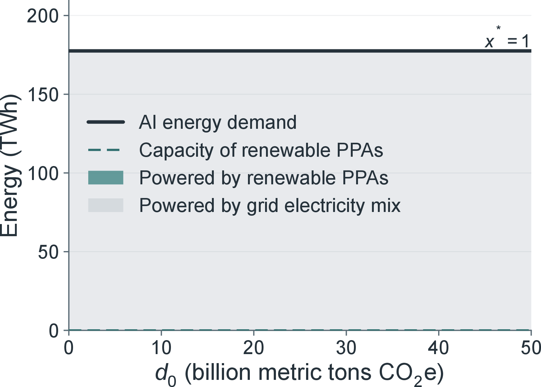
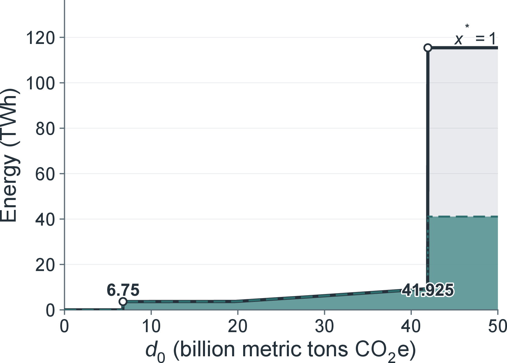
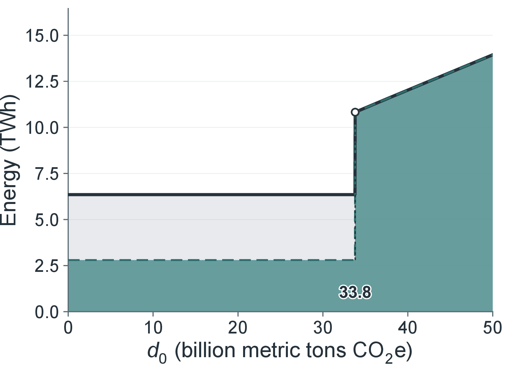
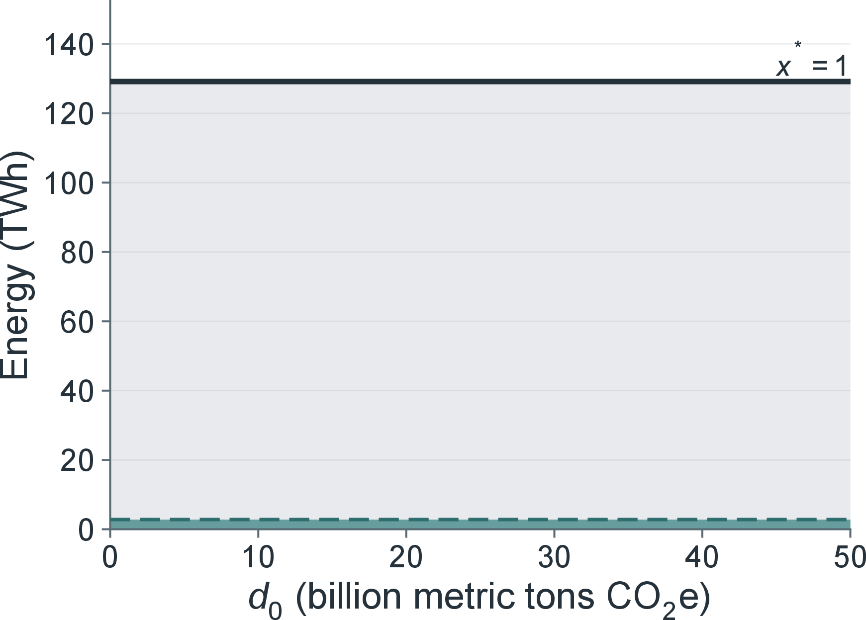
Figure 1: AI Energy Demand and Renewable Energy Investment Outcomes in the Case Study. Each panel plots AI energy demand and renewable PPA capacity against the baseline climate-damage scale \(d_0\); vertical scales differ across panels (peak demand ranges from about \(14\) TWh in Instance C to \(178\) TWh in Instance A). The developer’s equilibrium capability is \(x^*=1\) wherever marked; in the decoupling cases (Instances A and D), renewable PPAs meet a negligible share of AI energy demand (about \(0.02\%\) and \(2\%\), respectively). Circled markers denote critical values of \(d_0\): in panel (b), developer activation (\(6.75\)) and the adaptation-trap onset \(\bar{d}_m\) (\(41.925\)), beyond which equilibrium emissions are positive; in panel (c), the adaptation-pathway onset \(\bar{d}_c\) (\(33.8\)), beyond which equilibrium emissions are zero.. a — Market-led Scaling with Strong AI Investment (Instance A), b — Market-led Scaling with Limited AI Investment (Instance B), c — Resource-led Scaling with Limited AI Investment (Instance C), d — Resource-led Scaling with Strong AI Investment (Instance D)
6.2.1 High Market Potential: Decoupling.↩︎
Strong market potential can place the equilibrium in the decoupling zone under both market-led and resource-led scaling. Panels (a) and (d) of 1 illustrate the pattern: when \(\theta\) is high, the developer chooses frontier capability \(x^*=1\), yet renewable investment remains far below \(k\), so most AI electricity demand is met by the grid. Capability is then pinned down by market value rather than energy costs, leaving little scope for renewable investment to discipline scale. The policymaker therefore acts mainly through the composition effect, so differences between Instances A and D largely reflect renewable investment costs \(V(y)\) and grid generation costs \(c_f\).6 For the same reason, decoupling is relatively insensitive to \(d_0\): worsening climate raises adaptation value, but the associated welfare gains work through the scale channel, which is inactive once \(x\) is at its upper bound. This corresponds to [prop:1](ii) with \(\bar{d}_m=0\) (illustrated by panel (a)) and [prop:2](i) (illustrated by panel (d)).
Decoupling is also more likely to arise under market-led scaling. In numerical experiments holding other primitives fixed, the \(\theta\) threshold for decoupling is lower under market-led than under resource-led scaling, robust to the specific \(\lambda\) values in these scenarios. This accords with 4: market-led environments strengthen incentives to push to the frontier, so renewable investment is more likely to relax energy constraints without constraining capability.
6.2.2 Limited Market Potential: Coupling.↩︎
When AI market potential is limited, AI–energy coupling can arise in equilibrium. In 1, panels (b) and (c) show simultaneous increases in AI energy use and renewable PPA capacity for \(d_0\in[6.75,41.925]\) and for \(d_0\ge 33.8\), respectively. With a smaller market, energy costs become salient for the developer, which activates the scale effect in the policymaker’s renewable-investment problem. Whether coupling is temporary (and gives way to an adaptation trap) or instead persists as an adaptation pathway depends on the scaling regime, as illustrated in panels (b) and (c), which correspond to [prop:1](ii) and [prop:2](ii), respectively. In the ranges these two instances represent, market-led scaling tends to sustain frontier capability but fall short of net-zero, whereas resource-led scaling tends to deliver cleaner energy at the cost of frontier scale. These cases illustrate a practical trade-off between AI development and the clean-energy transition.
To interpret the transition points (\(d_0=41.925\) and \(33.8\) billion metric tons of CO\(_2\)e), we map emissions to atmospheric concentration using 1 ppm \(\approx\) 7.78 billion metric tons of CO\(_2\) [66]. The threshold in Instance B corresponds to about 6 ppm above the climate benchmark (roughly 2.3 years at recent rates of increase [67]); in Instance C, the pathway activates at about 4.3 ppm (about 1.7 years). These magnitudes place the model’s transition mechanisms in the near-term range given current trends. For example, the intensity of extreme events has risen markedly since 2020 [68]. Benchmarking current atmospheric CO\(_2\) (roughly 420 ppm) against 2020 levels (about 412 ppm) implies \(d_0\) on the order of 56 billion metric tons of CO\(_2\), exceeding both thresholds in panels (b) and (c).
6.3 Counterfactual Analysis: Levers for Net-Zero Frontier AI↩︎
We use the calibrated case study to ask what would deliver frontier capability on carbon-free power, that is, \(x^*(y^*)=1\) with \(y^*=k\). This outcome does not arise in the baseline calibrations. We therefore vary key primitives suggested by industry trends and quantify how each change shifts the equilibrium.
We start with renewable investment costs. In the market-led regime, condition (b) in [prop:1](i) gives a cost threshold below which the adaptation trap disappears and frontier AI can be powered without fossil generation. In our calibrations, the required decline is extremely large: at least 94.5% in Instance A and 72.1% in Instance B. Given the magnitude of recent cost declines, reductions of this size appear unlikely in the near term.
Condition (a) in [prop:1](i) highlights another lever: increasing frontier energy demand \(k\) relative to market investment \(\theta\) (see EC.2). A higher \(k/\theta\) makes clean capacity more valuable to the policymaker because it both displaces fossil electricity and relaxes the energy constraint that limits capability and adaptation benefits. This can bring net-zero frontier AI within reach in some environments. The [5] projects that AI electricity demand in China may rise by 170% from 2024 to 2030 (about 18% per year). In Instance B, an 18% increase in \(k\) moves the required renewable cost reduction into a feasible range when climate damages are sufficiently salient: a 25% cost reduction—within some projections [69]—is sufficient when \(d_0\ge 351.7\). However, the effect is fragile to rapid growth in \(\theta\): as investment rises relative to power needs, the economy returns to decoupling. In Instance B, this happens once \(\theta/k\) exceeds about 0.117 USD/kWh.
The same lever is largely ineffective in Instance A. Because the \(\theta/k\) threshold in condition (a) decreases in \(\lambda\) and increases in \(c_f\), the high-\(\lambda\), low-\(c_f\) configuration implies a very low threshold (about 0.057 USD/kWh). Even when coupling obtains, limited investment potential mutes the scale effect, while high energy demand makes clean expansion expensive. Consequently, coupling raises the required renewable cost reduction to 97.06% in Instance A. Net-zero frontier AI in such environments likely requires broader changes—a shift toward resource-led scaling, a clean-energy cost breakthrough, or policy that increases the effective price of fossil-based generation (e.g., stringent carbon pricing).
Instance C points in the opposite direction. In resource-led environments, coupling already operates through the adaptation pathway, so the binding constraint is the investment burden. Holding \(d_0=351.7\) as in the analysis of Instance B above, the nominal calibration requires a 41.71% reduction in renewable investment costs to reach net-zero frontier AI. Reducing \(k\) by 22.5% lowers this requirement to 13.5%, highlighting the value of data-center efficiency. But large cuts can break coupling: a 30% reduction returns the requirement to its nominal level.
Taken together, these counterfactuals imply that net-zero frontier AI is unlikely to follow from any single change. Achieving \(x^*(y^*)=1\) with \(y^*=k\) requires a portfolio: cheaper and easier-to-integrate clean capacity, policy that sufficiently internalizes climate damages, and management of AI-driven electricity demand consistent with the prevailing scaling regime. Even then, feasibility is limited in strongly market-led environments and hinges on the joint evolution of \(\theta\) and \(k\): rapid growth in investment or compute intensity can weaken coupling or raise the energy burden, shifting the equilibrium away from net-zero frontier AI.
7 Extensions↩︎
We extend the base model in two directions. First, AI capability may lower the cost of integrating renewables. Second, AI development may be competitive rather than monopolistic. Both extensions sharpen when the equilibrium tilts toward the adaptation trap versus the adaptation pathway. Hence, we focus on the market-led scaling scenario in this section.
7.1 AI-Enabled Reductions in Clean-Capacity Costs↩︎
The main model assumes renewable investment costs \(V(y)\) are independent of AI capability. In practice, higher capability can lower the cost of deploying and integrating renewables—in particular by improving forecasting, grid control, and storage operations, thereby easing integration frictions [2]. We capture this by allowing \[V=V(x,y), \qquad \frac{\partial V(x,y)}{\partial x}<0.\] One such specification is \[V(x,y)=\phi(x)\,V(y),\] where \(\phi'(x)<0\) and \(\phi(x)<1\) for all \(x\in(0,1]\), and \(V(y)\) is the baseline cost function used in the main model.
This extension introduces a feedback loop: higher \(x\) lowers the marginal cost of \(y\), strengthening incentives to invest in renewables, relaxing the energy constraint, and potentially supporting higher \(x\). As a result, full decarbonization is easier to sustain; in particular, the renewable-cost threshold for net-zero frontier AI is relaxed by a factor of \(\phi(1)\) (see EC.4.1).
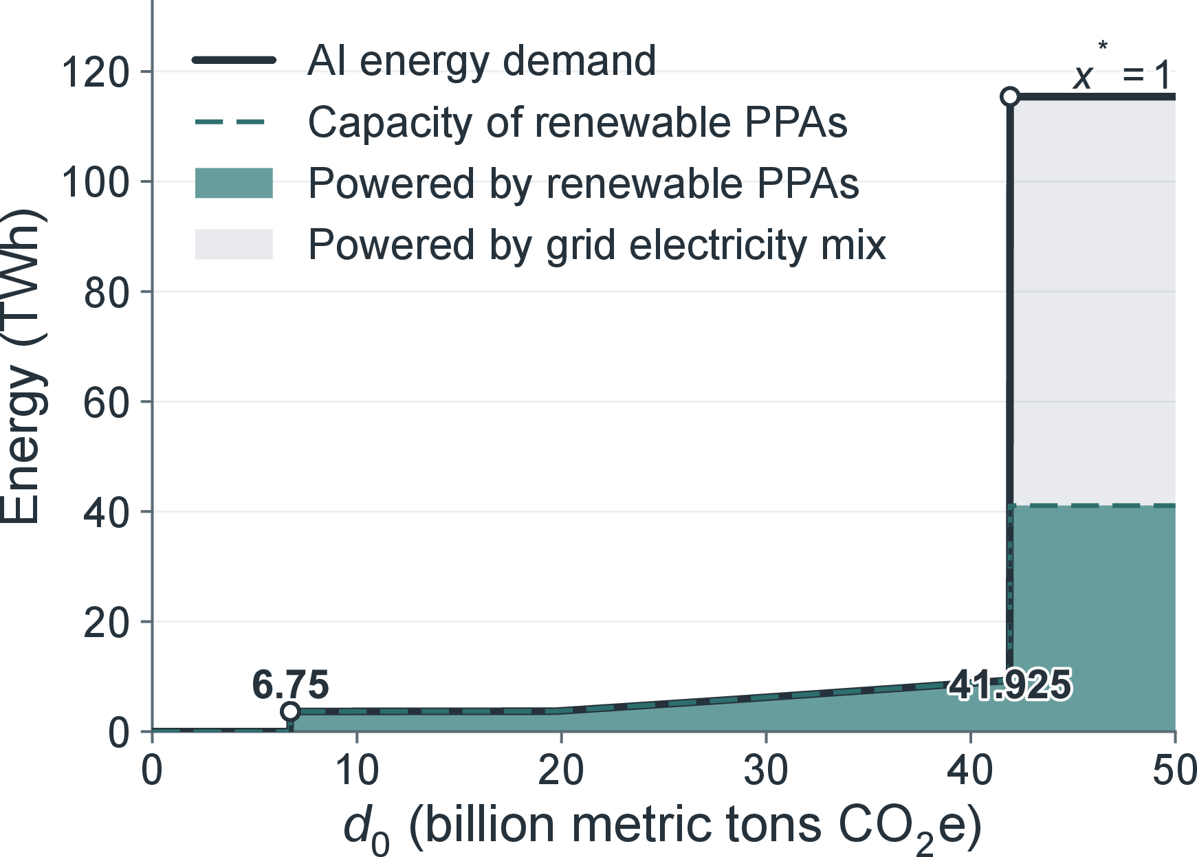
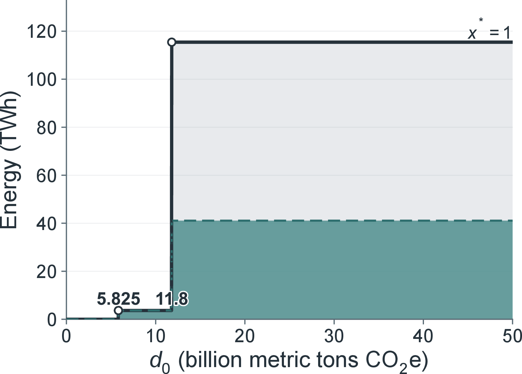
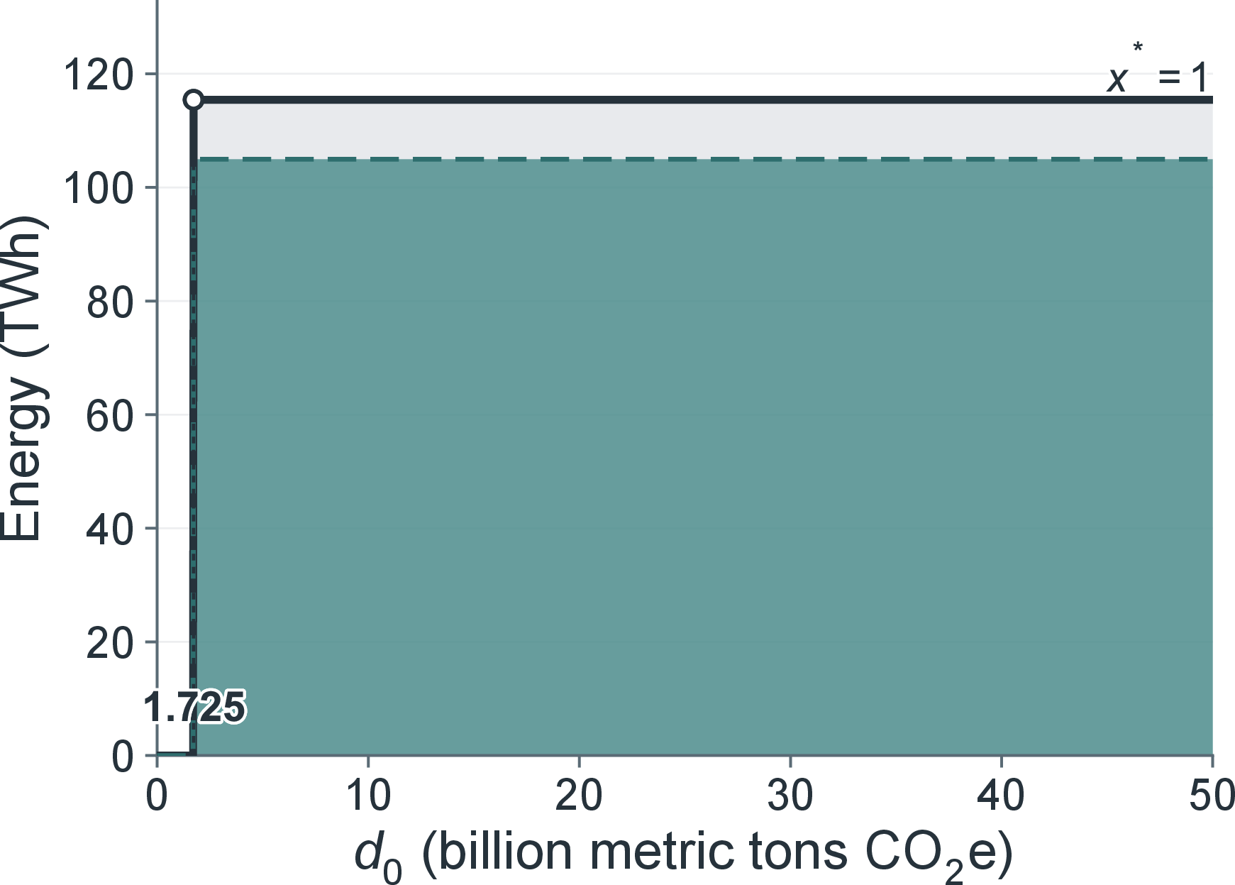
Figure 2: Adaptation Trap under AI-enabled Renewable Investment Cost Reduction. Illustration based on the parametric setting of Example B in the case study.. a — \(\phi(x)=1\) (the main model), b — \(\phi(x)=1-\frac{5}{9.83}x\), c — \(\phi(x)=1-\frac{7}{9.83}x\)
However, when AI-enabled cost reductions are insufficient to deliver full decarbonization, they can instead intensify the adaptation trap by expanding the parameter region in which the mechanism operates. 2 illustrates this pattern using Example B from the case study. With an AI-enabled cost-reduction potential of roughly \(50\%\) (panel (b)), an adaptation trap emerges once \(d_{0}\) reaches \(11.8\). This cutoff is far below the corresponding threshold in the absence of AI-enabled cost reduction, \(d_{0}=41.925\), shown in panel (a), which reproduces 1 (b) for comparison. Increasing the cost-reduction potential to \(70\%\) lowers the threshold further, as shown in panel (c). The intuition is straightforward: AI-enabled cost reductions strengthen the policymaker’s incentives to promote frontier AI development, thereby accelerating decoupling and, under market-led scaling, bringing forward the conditions under which the adaptation-trap mechanism arises.
Another key observation from comparing 2 (a) and (b) is that AI-enabled cost reductions may not translate into increased renewable capacity investment once the equilibrium enters the adaptation trap. This outcome arises from the loss of the scale effect as developers’ capability choices decouple from renewable availability. Consequently, only sufficiently large cost reductions can compensate for the loss of this lever and restore incentives for additional capacity investment. For Example B illustrated in 2, this cost-reduction requirement is at least 58%. If the threshold is met, AI-enabled cost reductions entail a trade-off in which the adaptation trap is more likely to occur but less fossil-dependent, as 2 (c) shows. Otherwise, such cost reductions tend to entrench carbon reliance by accelerating the same carbon-intensive trap, as is the case in 2 (b).
In practice, AI-enabled improvements in renewable development and integration are often cast as both an accelerant of the energy transition and a way to shrink AI’s own footprint. Our analysis shows that these gains depend on equilibrium responses: in some environments, efficiency improvements can deepen reliance on carbon-intensive supply rather than displace it. A decarbonizing AI–energy relationship requires more than technological complementarity: investment-side coupling must be sustained. In particular, policy may need to preserve the scale channel so that incentives for renewable capacity expansion keep pace with AI-driven electricity demand.
These effects are one instance of a broader pattern that spans the renewable-promoting levers available to a policymaker. We examine two further levers in [subsec:utilization] [subsec:decentralized]: a utilization factor \(\phi\) governing how much installed capacity becomes usable renewable energy, and decentralized investment in which the policymaker sets a financial incentive \(s\) based on which a utility chooses the capacity. Under market-led scaling, \(\phi\) and \(s\) reduce the carbon intensity of frontier AI yet can hasten the adaptation trap, lowering \(\bar{d}_m\) (for \(\phi\), only when it is not large enough to forestall the trap entirely). Under resource-led scaling, both uniformly reinforce the adaptation pathway, lowering \(\bar{d}_c\). The broader lesson is that making renewables cheaper, more usable, or better subsidized sharpens the incentive to scale capability, so the emissions consequences turn on the scaling regime rather than on the lever itself.
7.2 Competition Among AI Developers↩︎
The main model analyzes a single industry-representing developer. We extend the model to explore the implications of competition between developers. Specifically, we consider two AI developers that compete by choosing capabilities \((x_1,x_2)\) first and then prices \((p_1,p_2)\). We refer the reader to EC.4.2 for model details. We do note here that incorporating the price decision does not affect the main model results in the monopoly case, so the difference observed in this extension can be attributed to competition (see EC.4.2).
We observe that competition can reduce the private return to incremental capability, driven by two factors. First, market share is split so that the market potential (\(\theta\)) could be reduced for each developer. Second, the elasticity of revenue with respect to capability (\(\lambda\)) may decline, leading to slower growth, or even a reduction, in marginal revenue as the competitor scales as well. In reduced form, competition lowers the effective return from pushing to the frontier, which makes developers more sensitive to energy costs. As a result, equilibrium capability becomes more responsive to renewable capacity, and the planner’s renewable investment is more likely to discipline capability choices rather than be absorbed by additional fossil-powered scale. This potentially improves coupling and steers the equilibrium away from the adaptation trap.
A caveat, however, is that whether and to what extent this potential can be realized depends on the market condition. 3 illustrates a main finding based on extensive numerical experiments. When market investment potential (\(\theta\)) is high, the capability decision of either developer remains primarily driven by the market, and its coupling with renewable capacity enabled by competition is not strong enough to structurally shift the equilibrium. In this case, the equilibrium exhibits a “dual adaptation trap” under which both developers are subject to this mechanism. The dark blue region in 3 illustrates when such an equilibrium emerges; Example A in 6 turns out to be a case in point when \(d_0\) exceeds 32.78. However, competition still promotes renewable investment and reduces fossil usage in this case. For instance, in Example A (assuming \(d_0=50\)), the average percentage of AI energy demand satisfied by renewable investment (e.g., PPAs) increases from 0.02% to 4.93%.7

On the other hand, reduced market investment \(\theta\) may leave revenue potential insufficient to sustain competition, yielding a monopoly equilibrium (see the white region in 3). This outcome can arise for two reasons. First, when market elasticity with respect to capability (\(\lambda\)) is high, competition at the technological frontier becomes intense and can only be sustained in the presence of abundant renewable capacity, which turns out to exceed the policymaker’s investment in equilibrium. Second, competition may fail when overall market potential (\(\theta\)) is intrinsically low, such that even substantially lower renewable energy costs are insufficient to support multiple firms; Example B corresponds to this case.
Nevertheless, when \(\theta\) is intermediate and \(\lambda\) is not too high (see the light blue region in 3), competition can partially induce carbon-free AI development: in equilibrium, at least one developer’s energy demand is fully met by renewable resources despite market-led scaling. This case is more likely to occur when \(\lambda\) is reduced, that is, when market forces do not overly dominate cost considerations in scaling. This indicates that a decline in \(\lambda\)—for instance, as frontier gains moderate—tends to facilitate developer competition and differentiation, and thereby pushes part of the equilibrium into the carbon-free regime. Note that when \(\lambda\) drops below \(1+\alpha\), scaling becomes resource-led, which leads to the adaptation pathway. This extension highlights that an analogous mechanism may already be at work prior to this transition, operating through the competition lever.
A policy implication follows. Antitrust and market design in AI affect not only prices and innovation incentives but also the carbon intensity of the capability race. When rents are concentrated, a single developer has strong incentives to scale compute even under carbon-intensive power. When rents are contested, cost discipline rises, and renewable capacity becomes a more effective instrument for steering AI onto a carbon-free pathway.
8 Conclusion↩︎
AI and renewable energy are increasingly cast as a “power couple,” on the premise that surging AI demand will accelerate clean-energy investment and hasten decarbonization [9]–[11]. This paper asks when that premise holds and when it fails. Rather than taking renewable supply or AI demand as given, we treat capability choices and renewable-capacity expansion as jointly determined, and show that equilibrium outcomes hinge on two primitives: how compute maps into capability and how capability maps into private value.
A key insight from our analysis is that expanding renewable capacity need not decarbonize AI growth. When private returns to capability are supermodular and capability scales roughly proportionally with energy use, developers have strong incentives to push the frontier even when the marginal megawatt-hour is fossil-based. Anticipating this, the policymaker may invest less in renewables, because incremental clean capacity may not translate into a substantial increase in capability and, in turn, sufficient welfare gain that justifies investment costs. This regime supports a carbon-intensive equilibrium and an “adaptation trap”: as climate damages rise, the value of AI-enabled adaptation increases, which strengthens incentives to enable frontier scaling on fossil energy, thereby raising emissions. By contrast, when returns to additional capability are submodular and energy requirements rise steeply, energy costs become binding, and capability responds more directly to renewable capacity; clean investment then both enables capability and decarbonizes marginal compute, yielding an “adaptation pathway” in which adaptation advances through AI scaled on carbon-free power.
These regimes also clarify when “rebound” is benign and when it is harmful. Expanding renewable supply and improving energy efficiency both lower the effective cost of compute and can accelerate scaling. Under market-led scaling, this acceleration loosens the link between compute and clean capacity, slowing decarbonization and increasing the risk of carbon lock-in. Under resource-led scaling, the same cost reductions tighten that link, making renewable investment and AI growth mutually reinforcing. Carbon lock-in, therefore, can arise endogenously from incentives and scaling dynamics, not only from slow infrastructure or political inertia. A clean transition, on the other hand, is not guaranteed by ongoing renewable expansion, the cost advantage of clean power, or AI-driven efficiency improvements; it requires policies that keep clean capacity a binding constraint on marginal compute.
Four policy lessons follow. First, policies that expand clean capacity without addressing marginal emissions need not lower AI’s emissions intensity; policies that raise the private cost of fossil-powered compute can be instrumental, whether through carbon pricing, carbon-free procurement requirements, or constraints tied to local grid emissions. Second, to strengthen the coupling between AI growth and clean-energy deployment, policy must govern the conditions under which AI scales: the location and timing of large loads, renewable interconnection, and rules for carbon-free matching. Third, when market forces are exceptionally strong, energy policy may have limited leverage; expanding emissions reductions in other sectors to offset AI-related emissions may be more effective. Finally, the welfare value of AI’s adaptation potential is state-dependent: as climate damages rise, the planner’s optimal response can switch sharply between the trap and the pathway, implying that climate policy should treat adaptation and mitigation as a joint design problem.
Whether AI and renewable energy reinforce each other therefore depends on policy. The environmental consequences of AI are determined by the equilibrium response of the energy system and the institutions that govern it. Procurement, interconnection constraints, and the siting and timing of data-center expansion determine whether scaling is met by clean additions or by greater reliance on fossil generation. A clean scaling path requires policies and market design that sustain investment-side coupling so that renewable deployment keeps pace with compute growth. This, in turn, motivates a research agenda at the intersection of operations, markets, and political economy: measuring how workload flexibility affects marginal emissions; designing grid-aware siting and scheduling that internalize spatial and temporal system conditions; and studying how institutions such as PPAs, interconnection rules, capacity markets, and hourly matching requirements shape clean investment and the incentives to scale frontier AI.
Electronic Companion to
“Power Couple? AI Growth and Renewable Energy Investment”
9 Proofs of Technical Results↩︎
For convenience, we rewrite the developer’s profit in equation (2) as follows: Let \(\pi(x)\doteq \theta x^\lambda - c\cdot (kx^{1+\alpha})\). The developer’s profit equals \(\pi(x)\) where \(c=c_r\) if \(kx^{1+\alpha}\leq y\) (i.e., AI energy demand can be fully covered by renewable sources). We denote this piece by \(\pi_{c_r}(x)\). Otherwise, it equals \(\pi(x)\) where \(c=\beta c_r+(1-\beta)c_f\) where \(\beta=\frac{y}{kx^{1+\alpha}}\); this function can be rewritten as \(\theta x^\lambda - c_f\cdot (kx^{1+\alpha})+(c_f-c_r)y\), which we denote by \(\pi_{c_f}(x)\).
Proof of [lem:1]. The special case of this proposition in which \(\lambda=1+\alpha\) can be proven by setting \(y_1=y_2=0\) if \(\theta\geq c_fk\), setting \(y_1=y_2=k+1\) if \(\theta\leq c_rk\), and setting \(y_1=0, y_2=k+1\) if \(\theta\in (c_r,c_f)\).
To prove this proposition for the case in which \(\lambda>1+\alpha\), we first introduce two thresholds on \(\theta\): The first threshold is defined as \(\bar{\theta}\doteq \frac{(\alpha +1) c_f k}{\lambda }\). The second threshold, denoted by \(\bar{\bar{\theta}}\), is defined as follows: Consider the function \(F(\theta)=-\left((c_f-c_r) k^{\frac{\lambda }{-\alpha +\lambda -1}} \left(\frac{c_r}{\theta }\right)^{\frac{\alpha +1}{-\alpha +\lambda -1}}\right)+c_f k-\theta\). It can be shown that \(F''(\theta)<0\), indicating that \(F\) is concave and thus can have at most two zeros. It can be verified that one of them is \(c_rk\) because \(F(c_rk)=0\). Denote the other zero, if it exists, by \(\bar{\bar{\theta}}\).
We start by proving [lem:1] for the case in which \(\alpha=0\). In this case, \(\pi''(x)\geq 0\) under the assumption that \(\lambda>1+\alpha=1\), indicating that \(\pi(x)\) is convex and achieves its maximum at the boundary points. As such, we analyze two sub-cases.
The first sub-case is one in which \(\frac{c_r}{c_f}<\frac{1+\alpha}{\lambda}\) and \(\theta\in \left(\bar{\theta},\bar{\bar{\theta}}\right)\). Define \(y^0_1\doteq k^{\frac{\lambda }{-\alpha +\lambda -1}} \left(\frac{c_r}{\theta }\right)^{\frac{\alpha +1}{-\alpha +\lambda -1}}\). We also introduce another threshold \(y^0_2\): consider the function \(G(y)=\theta \left(\left(\frac{y}{k}\right)^{\frac{\lambda }{\alpha +1}}-1\right)-c_f k \left(\frac{y}{k}-1\right)\). It can be shown that \(G''(y)>0\), indicating that the function is convex. Furthermore, it can be verified that \(G(k)=0\) and \(G'(k)>0\) when \(\theta>\bar{\theta}\). This implies that in the first sub-case, \(G(y)\) has another zero that is strictly smaller than \(k\); denote that zero by \(y^0_2\). Hence, \(G(y)<0\) if and only if \(y\in (y^0_2,k)\).
We further prove that \(y^0_1<y^0_2\). We prove this by showing that \(G(y^0_1)>0\). It can be shown that \(G(y^0_1)=F(\theta)\). We show that \(\forall \theta\in (\bar{\theta},\bar{\bar{\theta}})\), \(F(\theta)>0\) is satisfied. We show this in two steps. First, we show that \(F(\theta)>0\) \(\forall \theta\in(c_rk,\bar{\bar{\theta}})\). This is because when \(\frac{c_r}{c_f}<\frac{1+\alpha}{\lambda}\), it can be calculated that \(F'(c_rk)>0\) and \(\lim_{\theta\rightarrow\infty}F(\theta)<0\), indicating that \(\bar{\bar{\theta}}\) exists and is greater than \(c_rk\), and \(F(\theta)>0\) if and only if \(\theta\in(c_rk,\bar{\bar{\theta}})\). Second, we show that \(c_rk<\bar{\theta}<\bar{\bar{\theta}}\) and thus \((\bar{\theta},\bar{\bar{\theta}})\subset (c_rk,\bar{\bar{\theta}})\). The inequality \(c_rk<\bar{\theta}\) directly follows from the condition that \(\frac{c_r}{c_f}<\frac{1+\alpha}{\lambda}\). To show \(\bar{\theta}<\bar{\bar{\theta}}\), we analyze \(F(\bar{\theta})\). It can be shown that \(F(\bar{\theta})=0\) when \(c_r=\frac{c_f(1+\alpha)}{\lambda}\); furthermore, it can be calculated that \(F(\bar{\theta})\) is strictly decreasing in \(c_r\) given \(\frac{c_r}{c_f}<\frac{1+\alpha}{\lambda}\) and \(\lambda>1+\alpha\). This indicates that \(F(\bar{\theta})>0\) and, in turn, \(\bar{\theta}<\bar{\bar{\theta}}\) holds, \(\forall c_r<\frac{c_f(1+\alpha)}{\lambda}\). This completes the proof that \(y^0_1<y^0_2\) in this sub-case. Accordingly, we can show the following.
When \(y<y^0_1\), it can be shown that (i) \(\pi_{c_r}(0)>\pi_{c_r}\left((y/k)^{1/1+\alpha}\right)\), and (ii) \(\pi_{c_f}(1)<\pi_{c_f}\left((y/k)^{1/1+\alpha}\right)\), indicating that the optimal technology choice is \(x=0\) due to the convexity of the functions \(\pi_{c_r}\) and \(\pi_{c_f}\). To prove (i), consider the function \(J(y)=\pi_{c_r}\left((y/k)^{1/1+\alpha}\right)-\pi_{c_r}(0)\). It can be shown that \(J''(y)>0\) and has two zeros \(y=0\) and \(y=y^0_1\). Hence, if and only if \(y\in (0,y^0_1)\), \(J(y)<0\), and thus (i) holds. To prove (ii), note that \(\pi_{c_f}\left((y/k)^{1/1+\alpha}\right)-\pi_{c_f}(1)\) is the \(G(y)\) function introduced above. Because \(G(y)>0\) \(\forall y<y^0_2\) and \(y^0_1<y^0_2\), (ii) is proven.
Based on the above observations, we know that when \(y\in [y^0_1,y^0_2)\), (i) \(\pi_{c_r}(0)\leq \pi_{c_r}\left((y/k)^{1/1+\alpha}\right)\), and (ii) \(\pi_{c_f}(1)<\pi_{c_f}\left((y/k)^{1/1+\alpha}\right)\), indicating that the optimal technology choice is \(x=(y/k)^{1/1+\alpha}\).
Similarly, when \(y\geq y^0_2\), we have (i) \(\pi_{c_r}(0)< \pi_{c_r}\left((y/k)^{1/1+\alpha}\right)\), and (ii) \(\pi_{c_f}(1)\geq \pi_{c_f}\left((y/k)^{1/1+\alpha}\right)\), indicating that the optimal technology choice is \(x=1\).
Hence, setting \(y_1=y_1^0\) and \(y_2=y_2^0\) proves [lem:1] in the first sub-case.
We then consider the second sub-case in which the condition in the first sub-case is not met.
(A) If \(\frac{c_r}{c_f}<\frac{1+\alpha}{\lambda}\) and \(\theta\leq \bar{\theta}\), then \(G'(k)\leq 0\), indicating that \(G(y)\geq 0\) and, accordingly, \(\pi_{c_f}\left((y/k)^{1/1+\alpha}\right)\geq \pi_{c_f}(1)\) holds \(\forall y\in [0,k]\). Hence, setting \(y_1=y_1^0\) and \(y_2=k\) proves the proposition.
(B) If \(\frac{c_r}{c_f}<\frac{1+\alpha}{\lambda}\) and \(\theta\geq \bar{\bar{\theta}}\), then \(G(y^0_1)=F(\theta)\leq 0\), which indicates that \(y^0_1\in (y^0_2,k)\). In that case, the solution \(x=(y/k)^{1/1+\alpha}\) is suboptimal. Hence, setting \(y_1=y_2=\frac{c_f k-\theta }{c_f-c_r}\) proves the proposition, because it can be shown that \(\pi_{c_r}(0)>\pi_{c_f}(1)\) if and only if \(y<\frac{c_f k-\theta }{c_f-c_r}\).
(C) If \(\frac{c_r}{c_f}\geq \frac{1+\alpha}{\lambda}\), it can be shown that \(\bar{\bar{\theta}}\leq c_rk\), thus \(F(\theta)>0\) if and only if \(\theta\in(\bar{\bar{\theta}},c_rk)\).
(C-i) If \(\theta\geq c_rk\), then \(F(\theta)\leq 0\), that is, \(G(y^0_1)\leq 0\), which is the situation discussed in (B).
(C-ii) If \(\theta<c_rk\), it can be shown that \(y_1^0>k\), indicating that \(J(y)\leq 0\) and, accordingly, \(\pi_{c_r}(0)\geq \pi_{c_r}\left((y/k)^{1/1+\alpha}\right)\) \(\forall y\in [0,k]\). Hence, the solution \(x=(y/k)^{1/1+\alpha}\) is also suboptimal. Hence, applying the approach in (B) and setting \(y_1=y_2=\frac{c_f k-\theta }{c_f-c_r}\) proves the proposition.
We then analyze the case in which \(\alpha>0\). It can be shown that \(\pi''(x)<0\) if \(x\leq \left(\frac{\theta (\lambda -1) \lambda }{\alpha (\alpha +1) ck}\right)^{\frac{1}{\alpha -\lambda +1}}\), and \(\pi''(x)\geq 0\) otherwise, indicating that \(\pi(x)\) is concave first and then becomes convex as \(x\) increases. Furthermore, it can be shown that \(\lim_{x\rightarrow 0} \pi'(x)<0\). These observations indicate that \(\pi(x)\) continues to achieve its maximum on the boundary points, and the arguments used to analyze the case in which \(\alpha=0\) continue to apply. Q.E.D.
Proof of [lem:2]. First consider the case in which \(\lambda\leq 1\). In this case, \(\pi''(x)=\theta (\lambda -1) \lambda x^{\lambda -2}-\alpha (\alpha +1) c x^{\alpha -1}\leq 0\), indicating that the function \(\pi(x)\) is concave. Hence, the global maximum of \(\pi(x)\) is achieved at its stable point. It can be shown that when \(y> k \left(\frac{\theta \lambda }{(1+\alpha) c_rk}\right)^{\frac{1+\alpha}{1+\alpha -\lambda}}\), the first piece \(\pi_{c_r}(x)\) achieves its global maximum (if it is less than 1), and the second piece \(\pi_{c_f}(x)\) decreases. For any \(y\in \left[k \left(\frac{\theta \lambda }{(1+\alpha) c_fk}\right)^{\frac{1+\alpha}{1+\alpha -\lambda}},k \left(\frac{\theta \lambda }{(1+\alpha) c_rk}\right)^{\frac{1+\alpha}{1+\alpha -\lambda}} \right]\), the first/second piece increases/decreases, thus the maximum is achieved at the break point at which \(x=\left(\frac{y}{k}\right)^{\frac{1}{1+\alpha}}\). For any \(y<k \left(\frac{\theta \lambda }{(1+\alpha) c_fk}\right)^{\frac{1+\alpha}{1+\alpha -\lambda}}\), the first piece increases, and the second piece achieves its global maximum (if it is less than 1). Incorporating the boundary constraint that \(x\leq 1\) leads to [lem:2] for this case.
We then consider the case in which \(\lambda>1\). In this case, it can be shown that \(\pi''(x)\geq 0\) if \(x<\left(\frac{\lambda(\lambda-1)\theta}{\alpha(1+\alpha)ck}\right)^{\frac{1}{1+\alpha-\lambda}}\) and \(\pi''(x)< 0\) otherwise, indicating that \(\pi\) is convex first and then becomes concave as \(x\) increases. Furthermore, \(\lim_{x\rightarrow 0}\pi'(x)=\lim_{x\rightarrow 0} \theta \lambda x^{\lambda -1}-(\alpha +1) c x^{\alpha }>0\), indicating that \(x=0\) cannot be the maximum. Therefore, \(\pi(x)\) continues to achieve its global maximum at a stable point, thus the arguments used in the previous case continue to apply. Q.E.D.
Proof of [prop:1]. Recall the \(y_1\) and \(y_2\) thresholds identified in [lem:1]. When \(V'(k)\leq \eta (c_f-c_r)+(1-b) e_f \xi\), it can be shown that either \(y^*<y_2\) or \(y^*=k\), in which case \(k(x^*(y^*))^{1+\alpha}\leq y^*\) is satisfied, indicating that \(E(x^*(y^*),y^*)=0\) always holds. To show this, assume that \(y^*\in (y_2,k)\). Then according to [lem:1], \(x^*(y^*)=1\). Plugging this solution into the policymaker’s welfare function, we obtain \(W(y^*)=\eta\left(-c_f(k-y^*)-c_ry^*+\theta\right)-\xi(1-b)(d_0+e_f(k-y^*))-V(y^*)\). It can be calculated that \(W'(y^*)=\eta(c_f-cr)+\xi(1-b)e_f-V'(y^*)\). Because \(V(y)\) is convex and \(y^*<k\), we have \(V'(y^*)<V'(k)\leq \eta (c_f-c_r)+(1-b) e_f \xi\), indicating that \(W'(y^*)>0\), which is a contradiction to the optimality of \(y^*\) as an interior solution.
When \(\theta\leq \max\{\frac{1+\alpha}{\lambda }\cdot c_fk, c_rk\}\), there are two sub-cases: (i) \(\frac{c_r}{c_f}<\frac{1+\alpha}{\lambda}\) and \(\theta\leq \frac{1+\alpha}{\lambda }c_fk\), which is the \(\bar{\theta}\) threshold defined in the proof of [lem:1], and (ii) \(\frac{c_r}{c_f}\geq \frac{1+\alpha}{\lambda}\) and \(\theta\leq c_rk\). Case (i) corresponds to situation (A) discussed in the second sub-case in the proof of [lem:1], in which \(y_2=k\) and thus the third scenario of \(x^*\) in [lem:1] does not materialize. Hence, \(k(x^*(y^*))^{1+\alpha}\leq y^*\) always holds. Case (ii) corresponds to situation (C-ii) discussed in the proof of [lem:1]. In that case, it can be shown that because \(\theta<c_rk\), \(y_1=y_2=\frac{c_fk-\theta}{c_f-c_r}>k\), indicating that \(x^*=0\) \(\forall y\in [0,k]\). Hence, \(k(x^*(y^*))^{1+\alpha}\leq y^*\) always holds as well.
Combining the above two paragraphs proves [prop:1](i).
Next consider the case in which neither condition in [prop:1](i) holds. This corresponds to either the first sub-case, or situations (B) and (C-i) in the second sub-case discussed in the proof of [lem:1]. In all of these cases, the third scenario of \(x^*\) in [lem:1] can materialize when \(y\) is sufficiently large, in particular, when \(y=k\). Hence, \(W(k)\), that is, the welfare function when \(y=k\), should be calculated by plugging in \(x^*(k)=1\). Based on the calculation in the first paragraph of this proof, we know that when \(V'(k)> \eta (c_f-c_r)+(1-b) e_f \xi\), \(W'(k)<0\), implying that \(y^*<k\). If \(y_2\leq 0\), then according to [lem:1], \(k(x^*(y))^{1+\alpha}>y\) holds for all \(y\in[0,k)\). Setting \(\bar{d}_m\) to be any negative number proves [prop:1](ii).
If \(y_2>0\), then \(W(y)\) can be formulated as a piecewise function containing at least two pieces: The last piece corresponds to the \(y\) range of \([y_2,k]\), in which \(x^*(y)=1\); we denote this piece by \(W_2\). At least one other piece corresponds to the first or second case of the \(x^*\) solution identified in [lem:1]. We show that \(y^*\) occurs on \(W_2(y)\) if and only if \(d_0\) is sufficiently large. It can be calculated that \(W_2''(y)<0\), indicating that \(W_2(y)\) is a concave function. Hence, if \(y^*\) occurs on \(W_2(y)\), then \(y^*\) equals either the stable point at which \(W_2'(y)=0\) (denoted by \(y'_2\)) or the endpoint \(y_2\) (because \(y^*<k\) as shown in the previous paragraph).
If \(\eta(c_f-c_r)+(1-b)e_f \xi-V'(y_2)>0\) (a condition independent of \(d_0\) because \(y_2\) is the zero of a function that is independent of \(d_0\); see the proof of [lem:1]), then \(W_2(y'_2)>W_2(y_2)\). Hence, \(y^*\) occurs on \(W_2(y)\) if and only if \(W(y)\leq W_2(y_2')\) holds for any \(y< y_2\). It can be calculated that for any \(y \leq y_2\), \(\frac{\partial(W(y)- W_2(y_2'))}{\partial d_0}\) equals either \(-b \xi\) (if the first case of \(x^*\) in [lem:1] materializes under \(y\), i.e., \(x^*(y)=0\)) or \(-b \xi \left(1-\left(\frac{y}{k}\right)^{\frac{1}{\alpha +1}}\right)\) (if the second case of \(x^*\) in [lem:1] materializes, i.e., \(x^*(y)=(\frac{y}{k})^{1/(1+\alpha)}\)). Because condition (i) in Proposition 3(i) does not hold, we know \(y_2<k\) according to the proof of [lem:1] (see the first sub-case, and situations (B) and (C-i) in the second sub-case). Hence, \(y<y_2\) implies that \(y<k\). Consequently, both derivatives calculated above are negative for any \(y<y_2\) given \(b>0\) (and are independent of \(d_0\)), indicating that \(W(y)- W_2(y_2')\) is a strictly decreasing linear function in \(d_0\). Hence, if \(y^*\) occurs on \(W_2(y)\) under some \(d'\), then the same happens under any \(d''>d'\), indicating that either [prop:1](i) or (ii) holds. To show that [prop:1](ii) holds in this case, define \(\Delta W(y)=W(y)- W_2(y_2')\) when \(d_0=0\) for any \(y<y_2\). Define \(\bar{d}''(y)=\max\{0,\Delta W(y)/|\frac{\partial(W(y)- W_2(y_2'))}{\partial d_0}|\}\), which is finite for any \(y<y_2<k\). By definition, \(W(y)<W_2(y_2')\) when \(d>\bar{d}''(y)\). Let \(\bar{\bar{d}}''=\max_{y<y_2}\bar{d}''(y)\). Then, when \(d>\bar{\bar{d}}''\), \(W(y)<W_2(y_2')\) \(\forall y<y_2\), and thus \(y^*=y_2'\), indicating that [prop:1](ii) holds in this sub-case if we set \(\bar{d}_m=\bar{\bar{d}}''\).
If \(\eta(c_f-c_r)+(1-b)e_f \xi-V'(y_2)\leq 0\), then \(W_2(y'_2)\leq W_2(y_2)\). Replacing \(y_2'\) by \(y_2\) in the arguments used in the previous bullet point proves [prop:1](ii) in this sub-case. Q.E.D.
Proof of [prop:2]. First consider the conditions in [prop:2](i): \(\theta\geq \frac{1+\alpha}{\lambda}c_fk\) indicates that \(k \left(\frac{\theta \lambda }{(1+\alpha) c_fk}\right)^{\frac{1+\alpha}{1+\alpha -\lambda}}\geq k\) given \(\lambda<1+\alpha\). In that case, \(x^*(y)=1\) \(\forall y\in [0,k]\) according to [lem:2]. Plugging \(x^*(y)=1\) into the welfare function leads to a function that we denote by \(\bar{W}_1(y)\). It can be calculated that \(\bar{W}_1''(y)<0\), indicating that \(\bar{W}_1(y)\) is a concave function. It can be calculated that when \(V'(k)>\eta(c_f-c_r)+(1-b) e_f \xi\), \(\bar{W}_1'(k)<0\) and thus \(y^*<k\). Hence, \(k(x^*(y))^{1+\alpha}=k> y^*\) for any \(d_0\). This proves [prop:2](i).
Next, consider the case in which the condition of [prop:2](i) is violated. Assume the first condition holds yet the second condition does not, that is, \(\theta\geq \frac{1+\alpha}{\lambda}c_fk\) and \(V'(k)\leq \eta(c_f-c_r)+(1-b) e_f \xi\). In this case, \(y^*=k\) based on the analysis in the previous paragraph. Hence, setting \(\bar{d}_c=0\) proves [prop:2](ii).
Assume the first condition is violated, that is, \(\theta<\frac{1+\alpha}{\lambda}c_fk\), indicating that \(k \left(\frac{\theta \lambda }{(1+\alpha) c_fk}\right)^{\frac{1+\alpha}{1+\alpha -\lambda}}< k\). In this case, the welfare function \(W(y)\) can be formulated as a piecewise function containing at least two pieces: The first piece corresponds to the \(y\) range of \([0,k \left(\frac{\theta \lambda }{(1+\alpha) c_fk}\right)^{\frac{1+\alpha}{1+\alpha -\lambda}})\), in which \(x^*=\left(\frac{\theta \lambda }{(\alpha+1)c_f k }\right)^{\frac{1}{1+\alpha -\lambda}}\); we denote this piece by \(W_1\). At least one other piece corresponds to the second or the third case of the \(x^*\) solution identified in [lem:2]. We show that \(y^*\) occurs on \(W_1(y)\) if and only if \(d_0\) is sufficiently small. It can be calculated that \(W_1''(y)<0\), indicating that \(W_1(y)\) is a concave function. Hence, if \(y^*\) occurs on \(W_1(y)\), then \(y^*\) equals either the stable point at which \(W_1'(y)=0\) (denoted by \(y_1'\)) or the endpoint \(y=0\).
If \(V'(0)< \eta(c_f-c_r)+(1-b) e_f \xi\) (a condition independent of \(d_0\)), then \(W_1(y_1')>W_1(0)\). Hence, \(y^*\) occurs on \(W_1(y)\) if and only if \(W(y)\leq W_1(y_1')\) holds for any \(y\geq k \left(\frac{\theta \lambda }{(1+\alpha) c_fk}\right)^{\frac{1+\alpha}{1+\alpha -\lambda}}\). It can be calculated that for any \(y\geq k \left(\frac{\theta \lambda }{(1+\alpha) c_fk}\right)^{\frac{1+\alpha}{1+\alpha -\lambda}}\), \(\frac{\partial(W(y)- W_1(y_1'))}{\partial d_0}\) equals either \(b \xi \left(\left(\frac{y}{k}\right)^{\frac{1}{\alpha +1}}-\left(\frac{\theta \lambda }{(1+\alpha)c_f k}\right)^{\frac{1}{\alpha -\lambda +1}}\right)\) (if the second case of \(x^*\) in [lem:2] materializes, i.e., \(x^*(y)=(\frac{y}{k})^{1/(1+\alpha)}\)) or \(b \xi \left(\left( \min\{\frac{\theta \lambda }{(1+\alpha)c_rk},1\}\right)^{\frac{1}{\alpha -\lambda +1}}-\left(\frac{\theta \lambda }{(1+\alpha)c_fk}\right)^{\frac{1}{\alpha -\lambda +1}}\right)\) (if the third case of \(x^*\) in [lem:2] materializes, i.e., \(x^*(y)=\min\{f(c_r),1\}\)). Both derivatives are positive for any \(y\geq k \left(\frac{\theta \lambda }{(1+\alpha) c_fk}\right)^{\frac{1+\alpha}{1+\alpha -\lambda}}\) given \(k \left(\frac{\theta \lambda }{(1+\alpha) c_fk}\right)^{\frac{1+\alpha}{1+\alpha -\lambda}}< k\) and \(b>0\) (and are independent of \(d_0\)), indicating that \(W(y)- W_1(y_1')\) is a strictly increasing linear function in \(d_0\). Hence, if \(y^*\) occurs on \(W_1(y)\) under some \(d'\), then the same happens under any \(d''<d'\), indicating that either [prop:2](i) or (ii) holds. To show that [prop:2](ii) holds in this case, define \(\Delta W(y)=W(y)- W_1(y_1')\) when \(d_0=0\) for any \(y\geq k \left(\frac{\theta \lambda }{(1+\alpha) c_fk}\right)^{\frac{1+\alpha}{1+\alpha -\lambda}}\). Define \(\bar{d}'(y)=\max\{0,-\Delta W(y)/\frac{\partial(W(y)- W_1(y_1'))}{\partial d_0}\}\). By definition, when \(d_0>\bar{d}'(y)\), \(W(y)>W_1(y_1')\), which implies that \(y^*\) no longer occurs on \(W_1(y)\). Setting \(\bar{d}_c=\min\{\bar{d}'(y), \forall y\geq k \left(\frac{\theta \lambda }{(1+\alpha) c_fk}\right)^{\frac{1+\alpha}{1+\alpha -\lambda}}\}\) proves [prop:2](ii) in this sub-case.
If \(V'(0)\geq \eta(c_f-c_r)+(1-b) e_f \xi\), then \(W_1(y_1')\leq W_1(0)\). Replacing \(y'_1\) by \(y=0\) in the arguments used in the previous bullet point proves [prop:2](ii) in this sub-case. Q.E.D.
10 Additional Results↩︎
In the counterfactual analysis in the case study (§6.3), we examine conditions under which an equilibrium in which the optimal AI capability choice is \(x^*(y^*)=1\) and the optimal renewable capacity investment is \(y^*=k\). Analytically, it can be shown that such conditions may involve (i) sufficiently low renewable investment cost, (ii) energy demand that is not excessively high, (iii) sufficiently adverse climate conditions. For simplicity, we adopt \(V(y)=g\cdot y^\mu\) where \(\mu>1\) in this analysis.
In the market-led scaling scenario, there exists an energy demand threshold \(\bar{k}\), a climate condition threshold \(\hat{d}\), and two marginal renewable investment cost thresholds \(g_1,g_2\) such that an equilibrium in which \(x^*(y^*)=1\) and \(y^*=k\) is achieved if (i) \(k\leq \bar{k}\), \(d_0\geq \hat{d}\) and \(g<g_1\) when \(\frac{\theta}{k}\leq \max\{\frac{c_f(1+\alpha)}{\lambda},c_r\}\), or (ii) \(g\leq g_2\) when \(\frac{\theta}{k}> \max\{\frac{c_f(1+\alpha)}{\lambda},c_r\}\).
Proof of [prop:EC1]. First, when \(\frac{\theta}{k}> \max\{\frac{c_f(1+\alpha)}{\lambda},c_r\}\), according to the fourth paragraph in the proof of [prop:1], \(x^*=1\) only materializes in the “decoupling zone” characterized by the third scenario in [lem:1]. Hence, achieving \(y^*=k\) requires \(V'(k)< \eta(c_f-c_r)+(1-b)e_f\xi\) according to the proof of [prop:1]. Setting \(g_2=\frac{\eta(c_f-c_r)+(1-b)e_f\xi}{\mu k^{\mu-1}}\) proves [prop:3](ii) in this case.
Second, when \(\frac{\theta}{k}\leq \max\{\frac{c_f(1+\alpha)}{\lambda},c_r\}\), according to the first paragraph in the proof of [prop:1], there are two possibilities.
\(\frac{c_r}{c_f}<\frac{1+\alpha}{\lambda}\) and \(\frac{\theta}{k}\leq \frac{1+\alpha}{\lambda }c_f\): in this case, \(y_2=k\). Hence, an equilibrium in which \(x^*(y^*)=1\) and \(y^*=k\) can only be achieved in the “coupling zone” in which \(x^*(y)=(\frac{y}{k})^{1/(1+\alpha)}\). Plugging this solution into the welfare function leads to a function that we denote by \(W_3(y)\). It can be shown that this equilibrium is indeed achieved if: (a) \(d_0\geq \frac{\eta \theta \lambda (\lambda- (1+\alpha))}{\alpha b \xi }\), (b) \(g\leq \min\{\frac{b d_0 \xi -(1+\alpha) c_r \eta k+\eta \theta \lambda }{(\alpha +1) k\cdot \mu k^{\mu-1}},\frac{b d_0 \xi -c_r \eta k+\eta \theta}{k^{\mu}}\}\). Condition (a) ensures that \(W_3(y)\) is concave, so the optimal solution is achieved either at a stable point or at the endpoint. Thus \(y^*=k\) when \(W_3'(k)\geq 0\), and \(W_3(k)\geq W(0)\) (i.e., renewable investment yields higher welfare than not investing). The two terms that define the \(g\) threshold in condition (b) ensure that these two inequalities hold.
\(\frac{c_r}{c_f}\geq \frac{1+\alpha}{\lambda}\) and \(\frac{\theta}{k}\leq c_r\): in this case, \(x^*(y)=0\) for any \(y\in[0,k]\). Hence, an equilibrium in which \(x^*(y^*)=1\) and \(y^*=k\) cannot be achieved. We impose \(k<\frac{\theta}{c_r}\) to eliminate this case.
Combining the conditions on \((k,d_0,g)\) proves [prop:3](i). Q.E.D.
Although it is intuitive that ensuring net-zero frontier AI requires a sufficiently low marginal cost of investment in renewables, Proposition [prop:3] indicates that the cost threshold depends on the ratio \(\frac{\theta}{k}\), which measures the average market investment per unit of energy demand. If this ratio exceeds \(\frac{c_f(1+\alpha)}{\lambda}\) (which is equivalent to \(\theta\lambda\geq c_fk(1+\alpha)\), i.e., the marginal market value exceeds the marginal cost at \(x=1\)), it can be shown that maximum AI capability is achieved in the decoupling zone, independent of whether \(y=k\). In this case, the reduction of the marginal cost of renewable investment is only driven by the composition effect, that is, it should be lower than the marginal benefit from displacing fossil fuel. Indeed, the proof shows that \(g_2\) equals the cost threshold identified in condition (b) in [prop:1](i).
Otherwise, maximum AI capability may be achieved in the coupling zone, which requires full decarbonization to justify its cost. In this case, the marginal benefit of renewable investment is determined by the scale effect, which includes the developer’s scale margin, the associated economic spillover, and the enhanced adaptation benefits, minus the renewable energy generation cost. These components determine the \((d_0,g_1)\) thresholds. A caveat is that in this case, the marginal benefit of renewable investment could be negative when frontier AI entails too high an energy cost even when powered by the cheaper renewable sources and therefore cannot be realized. This explains the upper bound on the energy demand \(k\) for this case. Another useful observation is that because the scale effect leverages AI’s adaptation benefits, the \(g_1\) bound can be much more relaxed than \(g_2\) when \(d_0\) is high, which suggests an avenue to circumvent the limited renewable investment cost reduction potential which is technology constraint.
We show that [prop:3] applies structurally to resource-led scaling scenarios. This is because the impact of the comparison between the elasticity parameters \(\lambda\) and \(\alpha\) is attenuated at frontier capability \(x=1\). The next proposition formalizes the finding.
In the resource-led scaling scenario, [prop:3] continues to hold if (a) the threshold on \(\frac{\theta}{k}\) that separates cases (i) and (ii) is changed to \(\frac{c_f(1+\alpha)}{\lambda}\), (b) the thresholds on \((k,d_0)\) are removed, and (c) the \(g_1\) threshold is replaced by a different one \(g_3\).
Proof of [pro:EC462]. Based on [lem:2], it can be shown that when \(\frac{\theta}{k}>\frac{c_f(1+\alpha)}{\lambda}\), \(f(c_f)>1\), thus only the first case (the “decoupling zone”) in [lem:2] materializes, in which \(x^*(y)=1\) for any \(y\in[0,k]\). Applying the same proof for [prop:3](ii) proves the result for the resource-led scaling scenario.
When \(\frac{\theta}{k}\leq \frac{c_f(1+\alpha)}{\lambda}\), \(f(c_f)\leq 1\), thus the welfare function has at least two pieces. Nevertheless, it can be shown that the equilibrium \(x^*=1\), \(y^*=k\) can only be achieved in the second case, that is, the “coupling zone” of [lem:2]. Plugging the \(x^*(y)=(\frac{y}{k})^{1/(1+\alpha)}\) solution into the welfare function leads to the same function \(W_3(y)\) as defined in the proof of [prop:3]. It can be proven that \(W_3(y)\) is guaranteed to be concave in the resource-led scaling scenario (thus the \(d_0\) threshold in [prop:3] is no longer needed). Meanwhile, we also plug the \(x^*=f(c_f)\) solution into the welfare function and denote the resulting function by \(W_4(y)\). Hence, \(y^*=k\) is achieved when (a) \(W_3'(k)\geq 0\), and (b) \(W_3(k)\geq \max_{y\in [0,kf(c_f)]}W_4(y)\). Condition (a) is equivalent to an upper bound on \(g\) as shown in the proof of [prop:3]. The same can be shown for condition (b): let \(y_4'\doteq \arg\max_{y\in [0,kf(c_f)]}W_4(y)\). Then condition (b) is equivalent to \(g(k^\mu-(y_4')^\mu)\) being no greater than a certain term that involves no \(g\). Since \(k^\mu-(y_4')^\mu\) is lower bounded by \(k^\mu-(kf(c_f))^\mu\), this condition can be translated into a well-defined upper bound on \(g\). Setting \(g_3\) as the minimum between this bound and the one that guarantees condition (a) proves the result for the case where \(\frac{\theta}{k}\leq \frac{c_f(1+\alpha)}{\lambda}\). Q.E.D.
11 Calibration Details↩︎
This section maps observable inputs into the parameter values used in Instances A–C. We proceed in three steps. First, we estimate the market-side relationship between investment and model capability to discipline the demand parameters. Second, we calibrate the technology scaling relationship linking capability to electricity use and anchor instance-specific energy-demand levels. Third, we set energy costs, emissions intensity, and the renewable investment cost function.
11.1 Market-side Calibration↩︎
We estimate the market scaling parameter \(\lambda\) by regression. Let \(w\) denote market willingness-to-pay. The power law \(w=\theta x^\lambda\) is equivalent to \(\log w = \lambda \log x+\log \theta\). For each instance, we assemble three annual observations of \((w,x)\) from AI investment and model capability measures for the U.S., China, and EU over 2023–2025, summarized in ¿tbl:tab:lambda95estimate?.
| United States | China | European Union | ||||
|---|---|---|---|---|---|---|
| 2-3 (lr)4-5 (lr)6-7 Year | Invest. | MMMU | Invest. | MMMU | Invest. | MMMU |
| 2025 | 341.80 | 85.4 | 76.25 | 80.1 | 22.10 | 62.5 |
| 2024 | 109.08 | 78.2 | 9.29 | 70.3 | 19.42 | 52.5 |
| 2023 | 67.22 | 59.4 | 7.76 | 45.9 | 11.00 | 45.6 |
Notes: Investment is in billions of USD. MMMU scores reflect the top-performing model in each region-year. See text for model names and data sources.
We construct the investment inputs in ¿tbl:tab:lambda95estimate? as follows. The 2023 and 2024 figures follow Maslej et al. (2024) and Maslej et al. (2025).8,9 For 2025, the investment value in Instance A is based on the volume of bonds issued by U.S.technology firms in 2025, which the source attributes largely to financing AI capability buildout.10 We verify that this measure is consistent with alternative estimates of U.S.AI investment in 2025.
For Instance C, the same source reports that European technology firms issued $49.1 billion in bonds in 2025. We treat this as a noisier proxy for AI development investment than its U.S.counterpart, because European firms are reported to emphasize AI applications (e.g., data management and optimization using AI tools) rather than frontier model R&D.11 Accordingly, we apply a scaling factor of 0.45 to isolate the portion plausibly attributable to AI development activities, yielding \(\theta = 49.1 \times 0.45 \approx 22.1\) billion USD in Instance C. The appropriate scaling factor is likely below 0.45, because some sources report substantially smaller figures when focusing on “core” AI development.12 Using such lower estimates preserves Instance C as a resource-led scaling scenario and does not materially change the numerical results.
For Instance B, the investment value is \(125 \times 0.61 \approx 76.25\), where 125 billion USD is total AI investment in China in 2025 and 61% is attributed to private investment.13 We use private investment to maintain comparability with the other investment measures, which are based on private-sector activity.
Model capability is measured by MMMU. The MMMU scores adopted for Instances A and B in ¿tbl:tab:lambda95estimate? are based on the highest MMMU (Val) evaluation reported for U.S.- and China-developed models in the corresponding year.14 The MMMU scores in Instance C are based on the performance of Mistral AI models reported in 202415 and 2025.16 No MMMU scores have been reported for Mistral’s 2023 models such as Mistral 7B Instruct. Mistral 7B Instruct achieved a score of 60.1 in the MMLU benchmark,17 while Pixtral 12B achieved 69.2.18 Assuming the same percentage increase in MMLU and MMMU scores between these two models, we estimate the MMMU score of Mistral 7B Instruct to be 45.6.
We set \(w\) to be the investment amounts and \(x\) to be the MMMU scores (normalized by 100 to lie in its range \([0,1]\)), and perform a linear regression for each instance. This yields a \(\lambda\) value of 3.83, 3.19, and 2.15.
The regression analysis also provides an estimate of \(\theta\), but it aggregates market conditions across 2023–2025 and does not target the 2024 conditions that underlie the remaining parameter choices. For consistency, we set the \(\theta\) values in Instances A and C to be the amounts of private AI investment in the U.S.and the EU in 2024 reported by Maslej et al. (2025). In China, public investment in AI plays a major role and is estimated to account for 39% of the total investment in 2025. We thus adjust China’s private AI investment figure reported by Maslej et al. (2025), which is 9.29 billion USD, and calculate the total investment to be \(9.29/(1-39\%)\approx 15.23\) billion USD, which is used as the \(\theta\) value in Instance B.
We estimate the \(\eta\) parameter using McKinsey’s project about the total economic value of Generative AI, which can be as high as 25.6 trillion USD worldwide. We divide that number by the revenue potential of the AI industry, of which the sum of the \(\theta\) values across the three instances is a reasonable proxy. This yields \(\eta = 25.6 \times 10^3/(109.08+15.23+19.42)\approx 178\).
The next subsection calibrates the technology scaling relationship between capability and energy use.
11.2 Scaling and Energy Demand↩︎
We calibrate the technology scaling parameter \(\alpha\) via regression. Let \(v\) denote the AI energy usage. The function \(v=kx^{1+\alpha}\) is equivalent to the linear function \(\log v = (1+\alpha)\log x +\log k\). We consider three sets of \((v,x)\) estimates in 2024, summarized in 1.
| United States | China | European Union | |
|---|---|---|---|
| Energy consumption (TWh) | 177.51 | 115.42 | 63.51 |
| MMMU score | 78.2 | 70.3 | 52.5 |
The energy consumption figures are based on estimates reported in Figure 2.12 by IEA (2025)19. The MMMU scores are the same as those shown in ¿tbl:tab:lambda95estimate?. Linear regression based on these estimates yields an \(\alpha \approx 1.467\).
Although the regression analysis also provides a \(k\) estimate, it does not account for the regional energy usage differences that we intend to capture through the different instances in the case study. To reflect such heterogeneity, we anchor the \(k\) estimate in each instance based on the actual energy consumption. In particular, the U.S.and China have actively engaged in frontier model development as illustrated by the corresponding MMMU scores. Hence, their energy consumption figures are reasonable proxies for the energy demand of frontier AI, reflecting regional differences such as compute capacity and energy efficiency. Therefore, we set the \(k\) value in Instances A and B to be the same as the 2024 energy consumption numbers in these two regions in 1, that is, 177.51 and 115.42 TWh, respectively. Nevertheless, the EU’s consumption figure may not fully represent its potential AI energy demand. We adjust this number by scaling it by a factor of \((70/52.5)^{1+1.467}\), effectively calculating the minimum amount of energy required if a model with an MMMU score above 70 is to be developed under the scaling law calibrated above. This yields \(k\approx 129.14\), which we adopt for Instance C.
The next subsection sets energy cost, emissions, and renewable investment parameters.
11.3 Energy Costs, Emissions, and Renewable Investment↩︎
We set \(c_r\) to be the lowest cost of a renewable PPA with 80% hourly matching, which is approximately 50, 48, and 65 USD per MWh according to Figure 2.19 by IEA (2025).
We estimate \(c_f\) based on the industry retail price range of grid electricity reported in Figure 2.19 by IEA (2025). This range is about \([79.27,93.90]\), \([87.80,150]\), and \([109.76,200]\) for the U.S., China, and EU, respectively (all numbers are in USD/MWh). Considering that the European range covers the entire EU and thus may be an overestimate of the volatility of the industry rates in data-center hubs (e.g., FLAP-D), we replace the lower bound (109.76) by the lowest industry rate relevant in the hub areas, which is approximately 164 USD/MWh (in France).20 We assume a uniform distribution of the grid rate, denoted by \(r_g\), in the ranges defined above. To reflect developers’ risk aversion to grid rate volatility, we adopt a mean–variance cost based on the following formula: \(c_f=E(r_g)+0.1Var(r_g)\). Accordingly, we can calculate \(c_f\) to be approximately 88, 151, and 193 USD per MWh in the three instances, respectively.
We next calibrate the renewable investment cost function \(V(y)\). We adopt a power-law formula for this cost function: \(V(y)=g\cdot y^\mu\). The calibration is based on solar farm investment costs in practice. To estimate \(\mu\), we collect investment information on major solar projects in China in recent years, summarized in ¿tbl:tab:solar?. Accordingly, it can be calculated that the average investment cost of existing solar capacities (i.e., those of the first three projects) is 0.60 billion USD/GW. The Ordos project will increase the total capacity by 94% and, at the same time, raise the average cost to 0.76 billion USD/GW, representing a 25% increase. Given cost function \(V(y)=g\cdot y^\mu\), the average investment cost is \(V(y)=g\cdot y^{\mu-1}\). Hence, the data collected implies \(1.94^{\mu-1}=1.25\). Solving this equation yields \(\mu\approx 1.34\).
| Midong | Mengxi Lanhai | Tianwan | Ordos | |
|---|---|---|---|---|
| Capacity (GW) | 3.5 | 3.0 | 2.0 | 8.0 |
| Investment (billion USD) | 2.13 | 1.60 | 1.40 | 7.33 |
| Grid connection | 2024 | 2024 | 2025 | 2027 (expected) |
To calibrate the \(g\) coefficient in the investment cost function, we collect prevailing solar investment cost information and find that 0.95, 0.59 and 0.72 USD per watt are reasonable estimates in the U.S., China, and EU.25\(^,\)26 Solar systems are expected to have a lifespan of approximately 30 years, with panels retaining at least 80% of their original power output and potentially remaining operational well beyond this period. Furthermore, solar installation costs are expected to further decrease in the future,27 so replacement cost is likely to be much lower compared to new installation cost. Hence, we amortized the installation cost by 60 years, obtaining an average cost of 15.83, 9.83, and 12 billion USD/TWh, which are set as the \(g\) values in Instances A-C, respectively.
Finally, we set \(e_f\) in Instances A-C to be the carbon intensity of the grid in the U.S., China, and EU, respectively, which is approximately 0.367 ton/MWh (calculated by dividing the total emission of 1.53 billion metric tons by the total generation of 4.18 trillion kilowatthours28), 0.614 ton/MWh,29 and 0.187 ton/MWh.30
12 Technical Details of Extensions↩︎
This section provides formal statements and supporting derivations for the extensions discussed in the main text. We first characterize how AI-enabled reductions in renewable investment costs affect the conditions for full decarbonization. We then present the model formulation for the competition extension and outline the solution approach.
12.1 AI-Enabled Reduction in Renewable Investment Costs↩︎
In this subsection, we formalize the finding that AI-enabled reduction in renewable investment costs reduces the cost requirement for achieving full decarbonization.
Given the renewable investment function \(\phi(x)V(y)\) where \(V(y)=g\cdot y^\mu\), [prop:3] continues to hold if the thresholds \(g_1\) and \(g_2\) are replaced by \(\frac{g_1}{\phi(1)}\) and \(\frac{g_2}{\phi(1)}\).
The proof follows that of [prop:3] except for replacing \(g\) with \(\phi(1)\cdot g\).
12.2 Competition Between AI Developers↩︎
We provide a detailed model formulation and technical details of the competition extension. We consider two symmetric developers that engage in capability and price competition by choosing \((x_1,x_2)\) first and then prices \((p_1,p_2)\).
Note that this setting extends the main model in two ways: first, the number of developers is increased; second, an additional pricing decision is introduced. To isolate the effects, we first show that extending the main model into a price-setting monopoly does not change the results. To meaningfully model the price decision, we introduce market heterogeneity by assuming the market willingness-to-pay parameter \(\theta'\) is uniformly distributed on \([0,\tilde{\theta}]\). The total demand is normalized to 1. Let \(p\) denote the monopolistic developer’s price decision. Accordingly, customers invest if \(\theta' x^\lambda\geq p\), indicating that the market demand equals \(\frac{\tilde{\theta}-px^{-\lambda}}{\tilde{\theta}}\), and the developer’s profit function becomes \(\tilde{\Pi}(x,y,p)=p\frac{\tilde{\theta}-px^{-\lambda}}{\tilde{\theta}}-\Big(\beta(x,y)c_r+\big(1-\beta(x,y)\big)c_f\Big)\,k\,x^{1+\alpha}.\) Optimizing this function over the price decision leads to \(\tilde{\Pi}^*(x,y)=\arg\max_{p\geq 0}\Pi(x,y,p)=\frac{\tilde{\theta}}{4}x^\lambda-\Big(\beta(x,y)c_r+\big(1-\beta(x,y)\big)c_f\Big)\,k\,x^{1+\alpha}\). It can be observed that \(\tilde{\Pi}^*(x,y)\) is the same as the developer’s profit function \(\Pi(x,y)\) formulated in the main model, except that \(\theta\) is replaced by \(\tilde{\theta}/4\). Therefore, we shall set \(\tilde{\theta}=4\theta\) in this extension to equate the equilibrium outcome from the price-setting monopoly and the main model so as to isolate the impact of competition.
We are now ready to formulate the duopoly extension. Let \(y_i\) be the amount of renewable investment capacity that developer \(i=1,2\) has access to. First consider the pricing stage: given \((x_1,x_2)\) (where \(x_1>x_2\) without loss of generality) and \((p_1,p_2)\), customers invest in \(x_1\) if their willingness-to-pay satisfies \(\theta' x_1^{\lambda }-p_1\geq \theta' x_2^{\lambda }-p_2\), which leads to \(\theta'\geq \frac{p_1-p_2}{x_1^{\lambda }-x_2^{\lambda }}\). Furthermore, for customers to make an investment, \(\theta' x_2^{\lambda}-p_2\geq 0\) should be satisfied, which gives \(\theta'\geq p_2 x_2^{-\lambda }\). Hence, let \(C(x,y)\doteq \Big(\beta(x,y)c_r+\big(1-\beta(x,y)\big)c_f\Big)\,k\,x^{1+\alpha}\) denote the energy cost under given \((x,y)\), then developer 1’s profit function equals \(\Pi_1(x_1,y_1,p_1,p_2]) = p_1 \left(\tilde{\theta}-\frac{p_1-p_2}{x_1^{\lambda }-x_2^{\lambda }}\right)/{\tilde{\theta}}-C(x_1,y_1)\). Developer 2’s profit function equals \(\Pi_2(x_2,y_2,p_1,p_2)=p_2 \left(\frac{p_1-p_2}{x_1^{\lambda }-x_2^{\lambda }}-p_2 x_2^{-\lambda }\right)/{\tilde{\theta}}-C(x_2,y_2)\). Maximizing these two profit functions together leads to a price equilibrium: \(p_1^*=\frac{2 x_1^{\lambda } \left(x_1^{\lambda }-x_2^{\lambda }\right)\tilde{\theta}}{4 x_1^{\lambda }-x_2^{\lambda }}\), and \(p_2^*= \frac{x_2^{\lambda } \left(x_1^{\lambda }-x_2^{\lambda }\right)\tilde{\theta}}{4 x_1^{\lambda }-x_2^{\lambda }}\). We plug the price equilibrium into the developers’ profit functions and analyze the capability choice equilibrium. This part of the analysis becomes analytically intractable. We resort to an extensive numerical study, which leads to the results shown in 7.2.
13 Additional Extensions↩︎
This appendix presents two further extensions that test the robustness of our main results to richer descriptions of how renewable capacity is financed and used. We first consider decentralized renewable investment, replacing the planner’s direct choice of capacity with an arrangement in which the policymaker sets a financial incentive and a utility makes the investment decision. We then consider imperfect renewable utilization, relaxing the assumption that installed capacity equals usable renewable energy to allow for intermittency, interconnection limits, or complementary infrastructure such as storage. In both cases, the adaptation-trap and adaptation-pathway characterizations of [prop:1] [prop:2] continue to hold, and the intensity of the policy or operational lever moderates the likelihood and severity of these outcomes in the same regime-dependent manner highlighted in the main text.
13.1 Decentralized Renewable Investment↩︎
In this extension, we explicitly model the interaction between policy choices and renewable capacity investment. We focus on a setting in which the policymaker provides financial incentives (e.g., renewable subsidies and tax credits), a major policy lever for stimulating renewable investment in practice. We also consider a utility undertaking renewable capacity development, reflecting one of the primary channels through which renewable energy investment occurs in practice.
The utility determines the renewable capacity level \(y\) to maximize the return from renewable investment. A stylized formulation of its objective is maximizing \((p_r-c_r+s)\cdot \beta(x^*(y),y) \cdot k(x^*(y))^{1+\alpha} - V(y)\), where \(p_r\) is the unit rate (e.g., a large load tariff) charged for the amount of renewable energy used by the developer under its optimal capability choices induced by \(y\), \(c_r\) is the unit renewable generation cost, and \(s\) is the unit financial incentive that the policymaker provides for renewable generation.31 While utilities may also recover part of their renewable investment costs from other ratepayers in practice, we abstract from these channels and focus on the direct interaction between renewable investment and AI development. In practice, electricity tariffs are typically subject to regulatory oversight and are therefore not readily adjusted especially compared to direct financial incentives such as subsidies or tax credits. Hence, we treat \(p_r\) as exogenous. We consider a three-stage game. In Stage 1, the policymaker chooses the financial incentive \(s\in [0,\bar{s}]\) where \(\bar{s}\) represents fiscal constraints that limit the amount of such incentive. The social welfare function that the policymaker aims to maximizes is the sum of the profit of the developer (plus associated economic spillovers) and the return to the utility (from renewable development), subtracts the climate damage and the fiscal spending on incentive provision. In Stage 2, the utility determines the renewable capacity level \(y\). Finally, in Stage 3, the developer chooses capability \(x\) given the available renewable capacity. Relative to the main model, the developer pays the renewable tariff \(p_r\) rather than \(c_r\), although we continue to assume \(p_r<c_f\), reflecting settings in which large-load renewable procurement provides electricity at a lower price than standard retail grid service.
We show that our main results are robust to the policy-investment interactions, and the likelihood as well as the magnitude of the adaptation/pathway effects can be moderated by the intensity of the policy support. We start by presenting this result for the market-led scaling scenario. Recall the \(y_1,y_2\) threshold that defines the developer’s optimal capability choice in [lem:1]. In the extension, we modify these thresholds by replacing \(c_r\) with \(p_r\) in their characterization (see the proof of [lem:1]) and denote the new thresholds by \(\hat{y}_1\) and \(\hat{y}_2\).
Statement (i) in [prop:1] continues to hold if either of the following conditions is satisfied: (a) \(\theta\leq \max\{\frac{1+\alpha}{\lambda }\cdot c_fk, p_rk\}\), (b) \(V'(k)\leq \min\{\eta (c_f-p_r)+(p_r-c_r)+(1-b) e_f \xi,p_r-c_r+\bar{s}\}\), or (c) \(V'(\hat{y}_2)>p_r-c_r+\bar{s}\).
Otherwise, statement (ii) in [prop:1] holds. Furthermore, the threshold \(\bar{d}_m\) decreases in \(\bar{s}\), whereas the equilibrium renewable energy investment \(y^*\) when \(d_0\geq \bar{d}_m\) increases in \(\bar{s}\).
Proof of [prop:ext2]. We can prove that condition (a) leads to statement (i) in [prop:1] based on the same arguments in the proof of [prop:1] (the second paragraph), because the developer’s capability choice follows [lem:1] with \(c_r\) replaced by \(p_r\). To prove condition (b), we complement the proof in [prop:1] (the first paragraph) by the fact that \(y^*=k\) can be achieved if and only \(V'(k)\leq p_r-c_r+\bar{s}\), i.e., there exists a \(s\) level to induce renewable investment to fully cover AI energy demand. Lastly, condition (c) indicates that under all feasible \(s\) levels, the induced renewable investment does not exceed the \(\hat{y}_2\) threshold and thus the equilibrium remains in the carbon-free zone.
To prove statement (ii) in [prop:1] continues to hold, we need to show that when the three conditions discussed above are violated, there are feasible \(s\) values under which \(x^*=1\) can materialize. This is guaranteed by \(V'(\hat{y}_2)\leq p_r-c_r+\bar{s}\). Furthermore, because \(V'(k)> \min\{\eta (c_f-p_r)+(p_r-c_r)+(1-b) e_f \xi,p_r-c_r+\bar{s}\}\), either (i) \(V'(k)> p_r-c_r+\bar{s}\) in which case no incentive level is sufficient to induce the utility to invest in \(k\) amount of renewable capacity, or (ii) \(V'(k)> \eta (c_f-c_r)+(1-b) e_f \xi\) in which case even when \(y=k\) is feasible, it is suboptimal (based on similar arguments in the fourth paragraph in the proof of [prop:1]). Hence, we know that when \(x^*=1\) is achieved, \(y<k\) is guaranteed under the optimal \(s\). Accordingly, let \(s^*\) be the optimal incentive level, and \(y^*(s^*)\) be the renewable investment induced. It can be shown that when \(y^*(s^*)\) occurs on \(W_2(y)\) which is defined in the proof of [prop:1], it equals either \(y_2\) or \(\hat{y}_2'\doteq \min\{y_2',(V')^{-1}(p_r-c_r+\bar{s})\}\). Replacing \(y'_2\) with \(\hat{y}_2'\) in the proof of [prop:1] proves that statement (ii) continues to hold in this extension. Furthermore, we know that \(\hat{y}_2'\) increases in \(\bar{s}\), and so does \(W_2(\hat{y}_2')\). Therefore, the threshold \(\bar{d}_m\) decreases in \(\bar{s}\) according to its definition (with \(y_2'\) replaced by \(\hat{y}_2'\)) in the proof of [prop:1]. This completes the proof of the sensitivity results in [prop:ext2](ii). Q.E.D.
[prop:ext2] indicates that policy support, when operating through the private investment incentives of renewable energy developers, may create a tradeoff between the timing and carbon intensity of an adaptation trap. While stronger policy support promotes renewable capacity investment and reduces the carbon intensity of AI development, it can simultaneously accelerate the attainment of frontier capability, thereby bringing forward the onset of the adaptation trap under the market-led scaling scenario.
Nevertheless, we show that stronger policy support can uniformly reinforces the adaptation pathway in the resource-led scaling scenario.
Statement (i) in [prop:2] continues to hold if either (a) \(\theta\geq \frac{1+\alpha}{\lambda}\cdot c_fk\) and \(V'(k)> \min\{\eta(c_f-p_r)+(p_r-c_r)+(1-b) e_f \xi, p_r-c_r+\bar{s}\}\) or (b) \(V'\left(kf(c_f)^{1+\alpha}\right)>p_r-c_r+\bar{s}\).
Otherwise, statement (ii) in [prop:2] holds. The threshold \(\bar{d}_c\) decreases in \(\bar{s}\) whereas and the equilibrium renewable energy investment \(y^*\) when \(d_0< \bar{d}_c\) is independent of \(\bar{s}\).
Proof of [prop:ext3]. To prove statement (i) in [prop:2] holds, we show that under either of the two conditions identified, only the first case of developer’s optimal capability choice \(x^*\) identified in [lem:2] can occur given a feasible incentive level; furthermore, the equilibrium renewable capacity investment \(y^*<k\). This holds under condition (b) because it implies that the investment threshold \(kf(c_f)^{1+\alpha}\) cannot be achieved by a feasible incentive level. To show the same under condition (a), we follow similar arguments in the first paragraph of the proof of [prop:2] if \(V'(k)> \eta(c_f-p_r)+(p_r-c_r)+(1-b) e_f \xi\). Otherwise, we know that \(V'(k)>p_r-c_r+\bar{s}\) must hold, which indicates that there does not exist a feasible incentive \(s\) that can induce renewable capacity investment at level \(k\), and thus \(y^*<k\) must hold as well.
To prove statement (ii) in [prop:2] holds when either condition is violated, we follow the proof of [prop:2] (from the second paragraph onward) by replacing \(c_r\) with \(p_r\). In particular, notice that because of the \(\bar{s}\) upper bound, the definition of the \(\bar{d}_c\) threshold should be changed to \(\bar{d}_c=\min\{\bar{d}'(y), \forall y\in [kf(c_f)^{1+\alpha} ,(V')^{-1}(p_r-c_r+\bar{s})]\}\), which decreases in \(\bar{s}\). However, the equilibrium renewable capacity investment before the adaptation pathway occurs, i.e., the optimal \(y^*\) that occurs on \(W_1(y)\) defined in the proof of [prop:2] does not change as long as \(V'\left(kf(c_f)^{1+\alpha}\right)\leq p_r-c_r+\bar{s}\) so that the entire \(W_1(y)\) piece is preserved in the extended model. Q.E.D.
13.2 Renewable Energy Utilization↩︎
The main model assumes that the renewable capacity investment is the same as the usable renewable energy level. In this extension, we allow these two quantities to differ to reflect operational factors that affect the realized utilization of renewable resources. Specifically, we model the amount of usable renewable energy by \(\phi\cdot y\) where \(\phi>0\) is the utilization factor. A \(\phi\) value in \((0,1)\) discounts the installed capacity, reflecting operational constraints such as intermittency and interconnection limitations. A \(\phi\) value that is greater than 1 indicates the existence of infrastructure or data center operations that complement renewable energy sources, such as energy storage systems or flexible workload scheduling practices. Accordingly, we modify the share of the developer’s energy demand met by renewables, originally formulated as the \(\beta(x,y)\) function in Equation (1) in the paper, to \(\tilde{\beta}(x,y)=\min\{\frac{\phi y}{kx^{1+\alpha}},1\}\). We then replace \(\beta(x,y)\) by \(\tilde{\beta}(x,y)\) in the model.
We solve the modified model and show the our main results continue to hold, although the moderating effect of the utilization factor \(\phi\) could differ across the market-led and resource-led scaling regimes. Proposition [prop:ext1] formalizes the findings.
Proof of [prop:ext1]. We first note that the modified renewables share function \(\tilde{\beta}(x,y)\) is equivalent to \(\beta(x,\phi y)\). Hence, by treating \(\phi y\) as one variable \(z\), the modified model is equivalent to the base model (with decision variables \(\{x,z\}\)) except that the renewable investment cost function \(V(y)\) should be replaced by \(\tilde{V}(z)\doteq V(\frac{z}{\phi})\). Hence, the proofs of [prop:1] and [prop:2] continue to apply to the extended model with the decision variable \(y\) replaced by \(z\), the corresponding threshold notation and expressions adjusted accordingly, and \(V(y)\) changed to \(\tilde{V}(z)\). In particular, we change \(V(k)\) to \(\tilde{V}'(k)=\partial V(\frac{z}{\phi})/\partial z|_{z=k}=\frac{1}{\phi}V'(\frac{z}{\phi})\). This completes the proof of [prop:ext1](i).
Next, we prove [prop:ext1](ii). To analyze the sensitivity of the adaptation trap threshold \(\bar{d}_m\) in [prop:1], we show that \(\tilde{V}(z)-\tilde{V}(z'_2)=V(\frac{z}{\phi})-V(\frac{z'_2}{\phi})\) increases in \(\phi\) for all \(z<z_2\) (\(z'_2\) and \(z_2\) defined in the same way as \(y'_2\) and \(y_2\) in the proof of [prop:1]). Specifically, given the convexity of the \(V\) function, it can be calculated that \(\partial \left(V(\frac{z}{\phi})-V(\frac{z'_2}{\phi})\right)/\partial \phi= \frac{1}{\phi^2}\left(z'_2V'(\frac{z'_2}{\phi})-zV'(\frac{z}{\phi})\right)>0\). Therefore, \(\Delta W(z)=W(z)-W_2(z_2')\) , which is the counterpart of the \(\Delta W(y)\) function defined in the proof of [prop:1] and equals a term independent of \(\phi\) minus \(\tilde{V}(z)-\tilde{V}(z'_2)\), decreases in \(\phi\). Consequently, the \(\bar{d}''(z)\) threshold, which is the counterpart of \(\bar{d}''(y)\) in the proof of [prop:1], decreases in \(\phi\) as well, and so does \(\bar{d}_m\) which is the maximum among \(\bar{d}''(z)\). Based on similar arguments, we show that \(\Delta W(z)\) as the counterpart of \(\Delta W(y)\) function defined in the proof of [prop:2] increases in \(\phi\). Hence, the adaptation pathway threshold \(\bar{d}_c\) in [prop:2] decreases in \(\phi\) according to how it is defined in the proof of [prop:2]. Q.E.D.
Proposition [prop:ext1] indicates that a higher \(\phi\) uniformly facilitates the adaptation pathway in the resource-led scaling regime: it not only enlarges the parametric region where an adaptation pathway exists (by decreasing \(\frac{1}{\phi}V'(\frac{k}{\phi})\) so the condition in [prop:2](i) is less likely to hold), but also accelerates the realization of such a pathway (by reducing the threshold \(\bar{d}_c\)). However, a higher \(\phi\) may not be universally beneficial in the market-led scaling regime. Notably, although a sufficiently large \(\phi\) reduces the likelihood of an adaptation trap (by making the condition in [prop:2](i) more likely to hold), when \(\phi\) is not large enough to eliminate the possibility of a trap altogether, an increase in \(\phi\) could conversely speed up the emergence of the trap (by reducing the threshold \(\bar{d}_m\)). While directionally distinct, the effects in the two scaling regimes stem from the same mechanism: more effective renewable utilization incentivizes more investment, thereby driving the equilibrium into the carbon-intensive zone in the market-led scaling regime or the carbon-free zone in the resource-led scaling regime.
References↩︎
AI may also help reduce emissions (mitigation), for example, by facilitating renewable integration or optimizing energy efficiency [2]. However, such effects are more uncertain (due to potential rebound effects) and slower to materialize, whereas adaptation benefits are more immediate and observable in practice. We focus on adaptation benefits as the primary social value of AI in the climate context.↩︎
In practice, developers’ alternative to grid power is likely a portfolio of energy resources, including dedicated renewable generation, efficient natural-gas technologies such as on-site combined cooling, heat, and power systems, and energy storage. We abstract from this mix and focus on the key economic and environmental attributes it typically delivers: lower generation costs and emissions than grid power, but at the expense of substantial upfront investment.↩︎
We acknowledge that grid capacity is constrained in practice. However, such constraints are typically reflected in interconnection queues for new data centers. Once connected, data centers generally rely on the utility’s obligation to serve, under which residual demand is met through grid power.↩︎
The model can be extended to include an existing renewable capacity level \(y_0\) in addition to the investment \(y\); all results remain robust.↩︎
In practice, the energy source can affect operations (e.g., workload shifting). We abstract from these operational margins to focus on investment and scaling incentives.↩︎
In Instance A, higher grid emissions are tempered by the strong adaptation value of frontier AI and are not decisive.↩︎
These percentages do not correspond to the overall percentage of renewable energy usage because the grid mix also contains a renewable component. Adopting the percentage of renewable generation in the U.S. grid (which is 21.4% in 2023), they correspond to an increase in AI’s overall renewable energy usage from 21.42% to 25.27%.↩︎
https://hai.stanford.edu/assets/files/hai_ai_index_report_2025.pdf. Figure 4.3.10. ↩︎
https://hai.stanford.edu/ai-index/2024-ai-index-report/economy. Second figure.↩︎
https://www.reuters.com/business/global-markets-tech-2025-12-22/↩︎
https://oecd.ai/en/wonk/measuring-ai-investment-new-oecd-ec-methodology↩︎
https://tech.eu/2025/11/04/europes-ai-ecosystem-rapid-growth-and-rising-global-ambitions/↩︎
https://www.secondtalent.com/resources/chinese-ai-investment-statistics/ ↩︎
https://llm-stats.com/models/mistral-small-3.2-24b-instruct-2506↩︎
https://docsbot.ai/models/compare/mistral-large/mistral-7b-instruct↩︎
https://iea.blob.core.windows.net/assets/601eaec9-ba91-4623-819b-4ded331ec9e8/EnergyandAI.pdf ↩︎
https://ec.europa.eu/eurostat/statistics-explained/index.php?title=Electricity_price_statistics. Figure 6. We note that, according to this source, the industrial electricity rate in Ireland exceeds the upper bound of 200 USD/MWh reported by the IEA (2025). Nevertheless, large data centers may be able to negotiate lower rates and benefit from tax incentives, potentially resulting in an effective electricity rate within the IEA range. Accordingly, we retain 200 USD/MWh as the upper bound.↩︎
https://www.pv-magazine.com/2024/06/06/worlds-largest-solar-plant-goes-online-in-china-2/↩︎
https://www.pv-magazine.com/2024/06/06/worlds-largest-solar-plant-goes-online-in-china-2/↩︎
https://www.saurenergy.com/solar-energy-news/construction-of-2gw-offshore-solar-plant-in-china-starts↩︎
https://www.reuters.com/business/energy/china-three-gorges-renewables-plans-11-bln-new-energy-project-inner-mongolia-2024-06-28/↩︎
https://a1solarstore.com/blog/what-is-a-solar-farm-and-how-much-money-can-it-make-you.html
https://compareelectricity.com/research/how-much-does-a-solar-farm-cost↩︎https://www.solarpowereurope.org/press-releases/new-study-reveals-path-to-reshore-solar
-manufacturing-in-europe. This article estimates that utility solar installations cost in Europe is about 60.8 €ct/Wp compared to 50.0 €ct/Wp for a Chinese system↩︎https://www.energy.gov/articles/doe-announces-goal-cut-solar-costs-more-half-2030↩︎
https://academic.oup.com/ijlct/article/doi/10.1093/ijlct/ctae181/7762370↩︎
See Figure 1 at https://www.eea.europa.eu/en/analysis/indicators/greenhouse-gas-emission-intensity-of-1.↩︎
Some renewable subsidies and tax benefits are tied to installed capacity rather than generation. This distinction does not affect the model outcomes because, in equilibrium, the developer either utilizes the full amount of available renewable generation or none of it.↩︎