Screened second-order exchange in the uniform electron gas:
exact reduction, a single-pole reference model and asymptotic analysis
March 24, 2026
Abstract
The uniform electron gas (UEG) is the basic reference system underlying the local-density approximation of density-functional theory. At high density the random-phase approximation (RPA) describes long-range screening well, but it misses the short-range, exchange-type correlation and leaves a systematic error in the correlation energy. A natural contribution that corrects this is the diagram obtained from the second-order exchange diagram by replacing one of its interaction lines with a frequency-dependent screened interaction; this is the screened second-order exchange (SOSEX). Here we evaluate this contribution explicitly within a model in which it can be treated analytically.
The reduction used here is based on exact multiplicative separation between the momentum variable \(q\) and the scaled frequency variable \(z=\xi/q\). Within the single-pole class considered here, this separation selects the case in which the characteristic screening-frequency scale is independent of momentum. We call the corresponding model the reduction-compatible single-pole (RC-SP) model. In that model the single-pole scale is denoted by \(\Lambda\), and the contribution is expressed as a one-dimensional integral depending on \(\Lambda\). The quantity obtained is not the correlation energy of the Coulomb system itself, but the contribution associated with the screened-second-order-exchange diagram. In the limit where the screened interaction returns to the bare Coulomb interaction (\(\Lambda\to\infty\)) this contribution reduces to the bare second-order exchange. We evaluate this limit in closed form and show that it agrees with the known value of the bare second-order exchange due to Onsager–Mittag–Stephen. This agreement provides a nontrivial check of the reduction and fixes an absolute energy scale for the \(\Lambda\)-dependence.
We analyze the dependence on the single-pole scale \(\Lambda\) by the Mellin–Barnes method and obtain asymptotic formulas in the small-\(\Lambda\) and large-\(\Lambda\) limits. Numerical evaluation is consistent with these formulas and shows a non-monotone dependence on \(\Lambda\): over an intermediate range, the normalized contribution exceeds its static-limit value. Finally, mapping \(\Lambda\) to the density parameter \(r_s\), these asymptotics generate specific functional forms in \(r_s\). Because these forms follow from the structure of the diagram rather than being chosen empirically, they can serve as a starting point for modeling screened-exchange contributions beyond the RPA.
1 Introduction↩︎
The practical success of density-functional theory (DFT) [1]–[4] rests on the accuracy of the exchange–correlation energy functional. The uniform electron gas (UEG) is the most widely used reference system for constructing exchange–correlation functionals within the local-density approximation (LDA) [2], [5]; most non-empirical LDA functionals are fitted as rational interpolations based on the Ceperley–Alder quantum Monte Carlo [6] and constrained to reproduce the known asymptotic forms in the high- and low-density limits [7]–[9]. This strategy works well, but the choice of analytic form is guided by empirical judgment rather than by diagrammatic structure. It is desirable to understand which perturbative contributions are essential in each density regime and what analytic forms they naturally generate.
At high density the random-phase approximation (RPA) captures long-range screening and collective excitations [10], but it lacks the short-range exchange-type contribution and leaves a systematic error in the absolute correlation energy [11]–[13]. The screened second-order exchange (SOSEX) correction is a natural candidate to remedy this, bridging the long-range screening of the RPA and the exchange-type correlation that the RPA omits. A complete treatment via the adiabatic-connection fluctuation–dissipation (ACFD) framework exists [11], [14], but the high-dimensional integrals make it difficult to extract the analytic structure of the correction in closed form. The aim of this paper is to evaluate the dynamically screened exchange diagram explicitly in a setting where it can be treated analytically, and to use the functional forms thus obtained as a guide for modeling screened-exchange contributions beyond the RPA.
The main contents of this paper are as follows.
First, we study the dynamically screened second-order exchange diagram for a general single-pole screening and identify the separation condition used by the one-dimensional reduction (Sec. 2). The essential point is the separation of the momentum variable \(q\) from the scaled frequency variable \(z=\xi/q\). Within the single-pole ansatz, exact multiplicative \(q\)–\(z\) separation selects the case in which the characteristic screening-frequency scale is independent of momentum. This is the reference model used here for the analytic treatment of the dynamically screened exchange diagram. For this model the contribution of the diagram reduces to the one-dimensional integral \[\tilde{\varepsilon}_{c}(\Lambda)=64\pi^{3}A_0\int_0^\infty K_\Lambda(y)\,\Phi(y)\,\mathrm{d}y, \label{eq:master}\tag{1}\] where \(\Lambda\) is the single-pole scale, \(K_\Lambda\) is the function determined by the screened interaction (the frequency integral) and \(\Phi\) by the geometry of the occupied states (the momentum integral) (derived in Sec. 3), and \(A_0\) is an overall conventional constant.
Second, we evaluate in closed form the static limit (\(\Lambda\to\infty\)) in which the screened interaction returns to the bare Coulomb interaction. In this limit the diagram reduces to the bare second-order exchange, and its value is \[\tilde{\varepsilon}_c(\infty)=64\pi^2A_0\,D_0,\qquad D_0:=\int_0^\infty\frac{\Phi(y)}{y}\,\mathrm{d}y =\frac{\pi^{3}}{18}\log2-\frac{\pi}{4}\zeta(3), \label{eq:D0intro}\tag{2}\] which we prove independently in Appendix 8. The ratio of the coefficients of \(\log2\) and \(\zeta(3)\) on the right-hand side coincides with the known value of the bare second-order exchange due to Onsager–Mittag–Stephen [15]. Therefore, fixing the overall constant \(A_0\) once so that the static limit agrees with this known value reproduces both coefficients simultaneously. This is not a separate fit of two independent coefficients; it is a confirmation that our reduction correctly yields this known result (\(D_0\) is moreover proportional to Glasser’s \(d=3\) constant [16]; Sec. 4).
Third, we analyze the dependence on the single-pole scale \(\Lambda\) by the Mellin–Barnes method and obtain asymptotic formulas in the small-\(\Lambda\) and large-\(\Lambda\) limits. Direct numerical evaluation is consistent with these asymptotic formulas and shows that the normalized contribution is non-monotone as a function of \(\Lambda\), exceeding its static-limit value over an intermediate range. Furthermore, mapping \(\Lambda\) to the density parameter \(r_s\), these asymptotics yield specific functional forms in \(r_s\) that serve as a starting point for modeling screened-exchange contributions beyond the RPA.
2 Screened second-order exchange and the setup↩︎
In this section we define screened second-order exchange at finite temperature, rewrite it as a zero-temperature imaginary-axis integral, isolate the \(q\)–\(z\) separability condition used by the reduction, and discuss the status and scope of this model quantity. We first give the definition and the overall constant \(A_0\). We define screened second-order exchange as the exchange-type second-order diagram in which one of the two interaction lines is replaced by a frequency-dependent screened interaction. Using the bosonic frequency \(\nu_\ell=2\pi\ell/\beta\), we consider the three-dimensional unpolarized UEG and nondimensionalize momenta by \(k_F\). The constant \(A_0\) collects the spin degeneracy, the \((2\pi)^{-3}\) of each momentum loop, the Coulomb coupling \(4\pi e^2\), the volume and particle-number normalization, and the convention factor between the grand potential and the energy: \[\Omega^{\mathrm{scr2x}}_T[D]=A_0\,\frac{1}{\beta}\sum_{\nu_\ell}\int \mathrm{d}^3q\, D(\boldsymbol{q},\mathrm{i}\nu_\ell)\,X_T(\boldsymbol{q},\mathrm{i}\nu_\ell), \label{eq:Omega}\tag{3}\] The chemical potential is denoted by \(\mu\), and \(n_F(x)=(\mathrm{e}^{\beta x}+1)^{-1}\) is evaluated at the one-particle energy measured from \(\mu\). Thus \[X_T=\int \mathrm{d}^3p\,\mathrm{d}^3k\,\frac{Q_T(\boldsymbol{p};\boldsymbol{q},\mathrm{i}\nu_\ell)\,Q_T(\boldsymbol{k};\boldsymbol{q},\mathrm{i}\nu_\ell)}{|\boldsymbol{p}-\boldsymbol{k}|^2},\quad Q_T(\boldsymbol{p};\boldsymbol{q},\mathrm{i}\nu_\ell)=\frac{n_F(\varepsilon_{\boldsymbol{p}}-\mu)-n_F(\varepsilon_{\boldsymbol{p}+\boldsymbol{q}}-\mu)}{\mathrm{i}\nu_\ell-(\varepsilon_{\boldsymbol{p}+\boldsymbol{q}}-\varepsilon_{\boldsymbol{p}})}. \label{eq:X}\tag{4}\] Here the chemical potential cancels from the denominator. In the zero-temperature fixed-density limit \(\mu\to\varepsilon_F\), the numerator therefore gives the occupation factor \(\Theta(1-|\boldsymbol{p}|)\) after momenta are scaled by \(k_F\). We write the zero-temperature limit as \(\tilde{\varepsilon}^{\,\mathrm{UEG}}_{\mathrm{scr2x}}[D]:=\lim_{T\to0}\Omega^{\mathrm{scr2x}}_T[D]/N\). The same imaginary-axis transfer kernel can also be obtained from the zero-temperature time-ordered Green-function expansion after the internal fermionic frequency is integrated out and the resulting transfer-frequency kernel is analytically continued off the real axis; this is summarized in Appendix 9.
We next move the finite-temperature Matsubara sum to a zero-temperature imaginary-axis integral. Writing the bosonic Matsubara sum as a contour integral, taking \(n_B(\omega)\to-\Theta(-\omega)\) as \(T\to0\) and Wick-rotating the negative real axis to the imaginary axis \(\omega=\mathrm{i}\xi\) (with \(\xi\in\mathbb{R}\) the resulting continuous imaginary-axis frequency replacing \(\nu_\ell\)), the UEG parity \(\Delta(-\boldsymbol{p}-\boldsymbol{q};\boldsymbol{q})=-\Delta(\boldsymbol{p};\boldsymbol{q})\), \(\delta(-\boldsymbol{p}-\boldsymbol{q};\boldsymbol{q})=-\delta(\boldsymbol{p};\boldsymbol{q})\) together with \(D(\boldsymbol{q},-\mathrm{i}\xi)=D(\boldsymbol{q},\mathrm{i}\xi)\) imply \(X(\boldsymbol{q},-\xi)=X(\boldsymbol{q},\xi)\). Thus, for the even integrand considered here, \[\frac{1}{\beta}\sum_{\nu_\ell} \longrightarrow \int_0^\infty\frac{\mathrm{d}\xi}{\pi}.\] With \(k_F=1\), \(\varepsilon_{\boldsymbol{p}+\boldsymbol{q}}-\varepsilon_{\boldsymbol{p}}=\boldsymbol{p}\cdot\boldsymbol{q}+q^2/2\), \(\Delta(\boldsymbol{p};\boldsymbol{q})=\Theta(1-|\boldsymbol{p}|)-\Theta(1-|\boldsymbol{p}+\boldsymbol{q}|)\) and \(\delta(\boldsymbol{p};\boldsymbol{q})=\boldsymbol{p}\cdot\boldsymbol{q}+q^2/2\), we obtain \[\begin{align} K[D]:=\tilde{\varepsilon}^{\,\mathrm{UEG}}_{\mathrm{scr2x}}[D] &=A_0\int_0^\infty\frac{\mathrm{d}\xi}{\pi}\int\mathrm{d}^3q\,D(\boldsymbol{q},\mathrm{i}\xi)\,X(\boldsymbol{q},\xi),\\ X(\boldsymbol{q},\xi)&=\int\mathrm{d}^3p\,\mathrm{d}^3k\,\frac{1}{|\boldsymbol{p}-\boldsymbol{k}|^2}\, \frac{\Delta(\boldsymbol{p};\boldsymbol{q})\Delta(\boldsymbol{k};\boldsymbol{q})}{[\mathrm{i}\xi-\delta(\boldsymbol{p};\boldsymbol{q})][\mathrm{i}\xi-\delta(\boldsymbol{k};\boldsymbol{q})]}. \end{align} \label{eq:KD}\tag{5}\]
We now consider general single-pole screening and isolate precisely the separability statement used in the reduction. For the single-pole family \[D_{1p}(\boldsymbol{q},\mathrm{i}qz)=D_q(q)\,\frac{u(q)^2}{u(q)^2+z^2},\qquad u(q)=\Omega_q/q,\] the reduction route used below becomes one-dimensional only after the screened interaction has been put into the multiplicatively separated form \(D(\boldsymbol{q},\mathrm{i}qz)=\widetilde{D}_q(q)\,w(z)\). For clarity, we spell out the short algebra behind this restriction. It concerns exact interaction-level separation only; it is not a general impossibility theorem for all possible indirect one-dimensional representations of special nonseparable models after the remaining integrations have been carried out. Suppose that, on an interval \(I\subset(0,\infty)\) where \(D_q(q)\ne0\) and \(u(q)>0\), one requires \[D_{1p}(q,\mathrm{i}qz)=\widetilde{D}_q(q)\,w(z)\] to hold for every \(q\in I\) and for more than one value of \(z\). Then, for any \(q_1,q_2\in I\), the ratio \(D_{1p}(q_1,\mathrm{i}qz)/D_{1p}(q_2,\mathrm{i}qz)\) must be independent of \(z\). Apart from a \(q\)-dependent prefactor this ratio contains \[\frac{u(q_1)^2}{u(q_2)^2}\, \frac{u(q_2)^2+z^2}{u(q_1)^2+z^2}.\] Independence of \(z\) at two distinct values of \(z\) forces \(u(q_1)^2=u(q_2)^2\), and hence \(u(q_1)=u(q_2)\) because \(u>0\). Thus the separation mechanism used in this paper selects a constant single-pole scale on \(I\). Conversely, if \(u(q)=\Lambda\), the separated form \(D_{1p}(q,\mathrm{i}qz)=D_q(q)\Lambda^2/(\Lambda^2+z^2)\) is immediate.
We therefore use the constant-scale single-pole model—which we call the reduction-compatible single-pole (RC-SP) model— \[D_{\mathrm{RC\text{-}SP}}(\boldsymbol{q},\mathrm{i}qz)=\frac{1}{q^2}\,\frac{\Lambda^2}{\Lambda^2+z^2} \label{eq:DRCSP}\tag{6}\] as the separable subfamily of the single-pole ansatz used for the one-dimensional kernel in this paper. In what follows we write the zero-temperature limit for this model—the left-hand side \(\tilde{\varepsilon}_c(\Lambda)\) of 1 in the Introduction—as \(\tilde{\varepsilon}_{c,\mathrm{RC\text{-}SP}}(\Lambda)\). Because \(u(q)\sim\omega_p/q\to\infty\) at long wavelength, the finite-\(\Lambda\) expansion is not uniform in the infrared, so RC-SP is not a surrogate for a realistic plasmon dispersion but an analytically tractable reference model. For general single-pole screening, the preceding formulae still give a useful route to finite-rank separable approximations built from the RC-SP kernel family (Sec. 7), but the exact one-variable kernel derived below is a property of the separated RC-SP case rather than a general classification of all possible reductions of screened interactions.
Finally, we make the status, scope and limitations of this model quantity explicit. First, the quantity that arises naturally in the finite-temperature formalism is the grand potential \(\Omega=E-TS-\mu N\), which differs from \(E\) by \(\mu N\) even as \(T\to0\). Hence the zero-temperature limit of 5 is not the correlation energy of the Coulomb system itself, but the contribution associated with the screened-second-order-exchange diagram. We do not assign to this quantity a completed parent approximation in the sense of Luttinger–Ward [17] or Almbladh–von Barth–van Leeuwen [18], and we deliberately distinguish it from the completed construction that derives the RPA correlation from the full adiabatic-connection fluctuation–dissipation framework [14]. Second, RC-SP is not a surrogate for a realistic plasmon-pole model (because of the infrared non-uniformity \(u(q)\to\infty\)) but an analytically tractable reference model that parameterizes dynamical screening by a single scale \(\Lambda\). Third, what is rigorously established here is (i) the exact reduction to a two-variable cosine-difference transform for general screening and the subsequent one-variable kernel for the separated Coulomb RC-SP case (Secs. 2 and 3), (ii) the closed form of the static geometric factor \(D_0\) (Proposition 1, Appendix 8), and (iii) the two-limit asymptotics of the screening factor with explicit remainder estimates (Sec. 5.4); the power-law mapping to \(r_s\) (Sec. 7.1) is a modeling choice. The significance of this paper is not to reproduce the entire correlation energy of the UEG, but to determine, for one contribution beyond the RPA, the functional forms constrained by the structure of the diagram, and to provide a controllable reference model for further analytic and numerical tests.
3 Reduction to a one-dimensional integral for the RC-SP model↩︎
Starting from 5 , we first derive a reduced formula valid for a general screened interaction in terms of a two-variable cosine-difference transform. We then specialize to the separated Coulomb RC-SP model, for which this formula becomes the one-dimensional integral 1 . We keep the overall numerical factors explicit.
We first set \(\xi=qz\). We then use two standard integral representations: the Fourier representation of the Coulomb kernel and a Schwinger parameter representation for each resolvent. Writing \(\boldsymbol{q}=q\hat{\boldsymbol{q}}\), \(\delta=q(\boldsymbol{p}\cdot\hat{\boldsymbol{q}}+q/2)\) and setting \(\xi=qz\) (\(\mathrm{d}\xi=q\mathrm{d}z\)), each resolvent produces a factor \(1/q\); together with \(\mathrm{d}^3q=q^2\mathrm{d}q\,\mathrm{d}\Omega_{\hat{\boldsymbol{q}}}\) the power of \(q\) is \(q^2\cdot q\cdot q^{-2}=q\). The coefficient remains \(A_0\): \[K[D]=A_0\int_0^\infty\frac{\mathrm{d}z}{\pi}\int_{S^2}\mathrm{d}\Omega_{\hat{\boldsymbol{q}}}\int_0^\infty \mathrm{d}q\,q\, D(\boldsymbol{q},\mathrm{i}qz)\,\tilde{X}(q,\hat{\boldsymbol{q}},z). \label{eq:Kqz}\tag{7}\] Here \(\tilde{X}(q,\hat{\boldsymbol{q}},z)\) is the momentum double integral \(X\) of 5 after the same substitution, i.e.with each resolvent denominator written as \(\mathrm{i}z-(\boldsymbol{p}\cdot\hat{\boldsymbol{q}}+q/2)\) (the two extracted factors of \(1/q\) being already accounted for above).
We decompose the Coulomb kernel by the identity \(\dfrac{1}{|\boldsymbol{p}-\boldsymbol{k}|^2}=\displaystyle\int\mathrm{d}^3r\,F_C(\boldsymbol{r})\mathrm{e}^{\mathrm{i}(\boldsymbol{p}-\boldsymbol{k})\cdot\boldsymbol{r}}\), \(F_C(\boldsymbol{r})=\dfrac{1}{4\pi|\boldsymbol{r}|}\), and in one block use the Schwinger representation together with the Fourier transform of the occupied sphere \(F_B(\rho)=4\pi j_1(\rho)/\rho=(2\pi)^{3/2}J_{3/2}(\rho)/\rho^{3/2}\) (\(j_1\) the spherical Bessel function of the first kind, \(J_{3/2}\) the Bessel function). The product-to-sum identity converts the two sine factors from the two blocks into a difference of cosines. Keeping this cosine-difference form is important: in the Coulomb case the individual cosine transforms need not converge, whereas their difference does. Folding the \(q\)-integral into \(\Psi_D(s_1,s_2;z):=\int_0^\infty\mathrm{d}q\,q\,D(q,\mathrm{i}qz)[\cos(qs_1)-\cos(qs_2)]\) gives the following expression, with the displayed coefficient including the product-to-sum factor and the \(1/\pi\) from 7 : \[\begin{align} K[D]&=\frac{2A_0}{\pi}\int_0^\infty\!\mathrm{d}z\int_{S^2}\!\mathrm{d}\Omega_{\hat{\boldsymbol{q}}}\int\!\mathrm{d}^3r\,F_C(\boldsymbol{r}) \int_0^\infty\!\mathrm{d}t_1\mathrm{d}t_2\,\mathrm{e}^{-z(t_1+t_2)} \\ &\quad\times \Psi_D\!\left(r_k+\frac{t_1-t_2}{2},\frac{t_1+t_2}{2};z\right) F_B(\boldsymbol{r}+t_1\hat{\boldsymbol{q}})F_B(\boldsymbol{r}-t_2\hat{\boldsymbol{q}}). \end{align}\]
We next perform the central affine transformation. With \(y=t_1+t_2\), \(x=(t_2-t_1)/(t_1+t_2)\), \(\boldsymbol{r}=y(\boldsymbol{R}+\tfrac x2\hat{\boldsymbol{q}})\) we have \(\mathrm{d}t_1\mathrm{d}t_2=\tfrac y2\mathrm{d}x\mathrm{d}y\), \(\mathrm{d}^3r=y^3\mathrm{d}^3R\), \(a=|\boldsymbol{R}+\tfrac12\hat{\boldsymbol{q}}|\), \(b=|\boldsymbol{R}-\tfrac12\hat{\boldsymbol{q}}|\), \(r_k+\tfrac{t_1-t_2}{2}=yR_k\), \(\tfrac{t_1+t_2}{2}=\tfrac y2\). Since \(F_BF_B=(2\pi)^3J_{3/2}(ay)J_{3/2}(by)/(y^3a^{3/2}b^{3/2})\), the \(y^{-3}\) cancels against \(\mathrm{d}^3r=y^3\mathrm{d}^3R\) and the coefficient becomes \(\dfrac{2A_0}{\pi}\times(2\pi)^3\times\dfrac12=8\pi^2A_0\): \[\begin{align} K[D]=8\pi^2A_0\int_0^\infty\!\mathrm{d}z\int_{S^2}\!\mathrm{d}\Omega_{\hat{\boldsymbol{q}}}\int\!\mathrm{d}^3R\int_{-1}^1\!\mathrm{d}x\int_0^\infty\!\mathrm{d}y\; y\,\mathrm{e}^{-zy}\,&F_C\!\Big(y\big(\boldsymbol{R}+\tfrac x2\hat{\boldsymbol{q}}\big)\Big)\\ &\times\Psi_D\!\Big(yR_k,\tfrac y2;z\Big)\, \frac{J_{3/2}(ay)J_{3/2}(by)}{a^{3/2}b^{3/2}}. \end{align} \label{eq:Kaffine}\tag{8}\]
We then use the RC-SP separation and a Frullani integral. For RC-SP we separate \(\Psi_D=w_\Lambda(z)\Psi_{D_q}\), \(w_\Lambda(z)=\Lambda^2/(z^2+\Lambda^2)\). Defining the one-variable kernel \[K_\Lambda(y):=\frac{1}{\pi}\int_0^\infty w_\Lambda(z)\mathrm{e}^{-zy}\mathrm{d}z=\frac{1}{\pi y}\Xi(\Lambda y),\qquad \Xi(z)=z\int_0^\infty\frac{\mathrm{e}^{-zt}}{1+t^2}\mathrm{d}t \label{eq:KLambda}\tag{9}\] and applying \(\int_0^\infty w_\Lambda(z)\mathrm{e}^{-zy}\mathrm{d}z=\pi K_\Lambda(y)\) to the \(z\)-integral of 8 makes the coefficient \(8\pi^2A_0\times\pi=8\pi^3A_0\). For the Coulomb part, the Frullani formula \(\int_0^\infty\frac{\cos aq-\cos bq}{q}\mathrm{d}q=\log\frac{b}{a}\) gives \(\Psi_{D_q}(yR_k,\tfrac y2)=\log\frac{1}{2|R_k|}\), the \(y\) in \(F_C(y(\cdots))=\frac{1}{4\pi y|\boldsymbol{R}+\frac{x}{2}\hat{\boldsymbol{q}}|}\) cancels against \(\int\mathrm{d}y\,y\), and with \(\int_{S^2}\mathrm{d}\Omega_{\hat{\boldsymbol{q}}}=4\pi\), \(\hat{\boldsymbol{q}}\to\hat{\boldsymbol{e}}\) the coefficient factor is \(8\pi^3A_0\times4\pi\times\frac{1}{4\pi}=8\pi^3A_0\): \[\tilde{\varepsilon}_{c,\mathrm{RC\text{-}SP}}(\Lambda)=8\pi^3A_0\int\!\mathrm{d}^3R\int_{-1}^1\!\mathrm{d}x\int_0^\infty\!\mathrm{d}y\, K_\Lambda(y)\,\frac{\log(1/(2|R_k|))}{|\boldsymbol{R}+\tfrac x2\hat{\boldsymbol{e}}|}\,\frac{J_{3/2}(ay)J_{3/2}(by)}{a^{3/2}b^{3/2}}. \label{eq:specialized}\tag{10}\]
Finally we extract the geometric block \(\Phi(y)\) and obtain the total coefficient \(64\pi^3A_0\). In cylindrical coordinates about the \(\hat{\boldsymbol{e}}\) axis, write \(R_\parallel=\boldsymbol{R}\cdot\hat{\boldsymbol{e}}\). The \(x\)-integral gives \(\int_{-1}^1\mathrm{d}x/|\boldsymbol{R}+\tfrac x2\hat{\boldsymbol{e}}|=2\log\frac{R_\parallel+1/2+a}{R_\parallel-1/2+b}\). In prolate-spheroidal coordinates \(u=a+b\in[1,\infty)\), \(v=a-b\in[-1,1]\) (\(\mathrm{d}^3R=\frac{1}{8}(u^2-v^2)\mathrm{d}u\mathrm{d}v\mathrm{d}\phi\), \(R_\parallel=\tfrac{uv}2\)) we have \(2\log\frac{R_\parallel+1/2+a}{R_\parallel-1/2+b}=2L(u)\), \(L(u)=\log\frac{u+1}{u-1}\), and \(\log\frac{1}{2|R_\parallel|}=\log\frac{1}{|uv|}\). From \(J_{3/2}(w)=\sqrt{2w/\pi}j_1(w)\) we get \(\frac{J_{3/2}(ay)J_{3/2}(by)}{a^{3/2}b^{3/2}}=\frac{2y}{\pi ab}j_1 j_1\), \(ab=(u^2-v^2)/4\), so \((u^2-v^2)\) cancels. The \(\phi\)-integral gives \(2\pi\) and, being even in \(v\), we fold onto \(v\in[0,1]\). Collecting the numerical factors explicitly, \(2\pi\cdot\frac{1}{8}\cdot2\cdot\frac{8}{\pi}\cdot2=8\), so that \(\Phi^{\mathrm{corr}}_0(y)=8\Phi(y)\), with \[\Phi(y):=y\int_1^\infty\!\mathrm{d}u\,L(u)\int_0^1\!\mathrm{d}v\,\ell(u,v)\, j_1\!\Big(\tfrac{u+v}{2}y\Big)j_1\!\Big(\tfrac{u-v}{2}y\Big),\quad \ell(u,v)=\log\frac{1}{uv}. \label{eq:Phi}\tag{11}\] Since \(\tilde{\varepsilon}=8\pi^3A_0\int K_\Lambda\Phi^{\mathrm{corr}}_0\mathrm{d}y\), the total coefficient is \(8\pi^3A_0\times8=64\pi^3A_0\), giving 1 . For the Coulomb RC-SP model, this reduces the diagram 5 to the one-dimensional integral 1 .
4 Static limit and agreement with bare second-order exchange↩︎
From \(\Xi(z)\to1\) (\(z\to\infty\)) we have \(K_\Lambda(y)\to1/(\pi y)\), hence \(\tilde{\varepsilon}_{c,\mathrm{RC\text{-}SP}}(\infty)=64\pi^2A_0D_0\), \(D_0=\int_0^\infty\Phi(y)/y\,\mathrm{d}y\). In the static limit both interaction lines become bare Coulomb, and the diagram reduces exactly to the topology of the bare second-order exchange.
Proposition 1 (Closed form of the static geometric factor). For \(\Phi\) of 11 , \(D_0=\dfrac{\pi^{3}}{18}\log2-\dfrac{\pi}{4}\zeta(3)=-\dfrac{\pi}{6}G(3)=0.2499018971\ldots\), with \(G(3)=\dfrac32\zeta(3)-\dfrac{\pi^{2}}{3}\log2\).
The complete proof is given in Appendix 8. It does not rely on Glasser’s evaluation and is self-contained: after the \(y\)-integral is performed, the remaining integrals are reduced to logarithmic, dilogarithmic and unit-interval logarithmic and polylogarithmic integrals. The constants needed for this reduction are derived in Lemma 6 from elementary series and standard polylogarithm identities, rather than taken from external integral tables. The argument has three steps. (i) Performing the \(y\)-integral with the Weber–Schafheitlin-type formula \(\int_0^\infty j_1(ay)j_1(by)\mathrm{d}y=\frac{\pi b}{6a^2}\) (\(a\ge b\), \(j_1\) the spherical Bessel function), the inner \(v\)-integral closes in terms of \(\mathop{\mathrm{Li}}_2\) through an elementary function \(h(u)\), giving \(D_0=\frac{\pi}{3}\int_1^\infty L(u)h(u)\mathrm{d}u\). (ii) The substitution \(u=1/x\) maps the remaining integral to the unit interval. Reorganizing it through \(\Psi(x)=\big[\log x\log(1+x)-\mathop{\mathrm{Li}}_2(-x)\big]/x\) makes the integrations by parts well behaved at the endpoints and gives \(\int_1^\infty L(u)h(u)\mathrm{d}u=\frac{\pi^2}{6}\log2-\frac{3}{4}\zeta(3)\). (iii) Hence \(D_0=\frac{\pi^3}{18}\log2-\frac{\pi}{4}\zeta(3)=-\frac{\pi}{6} G(3)\). This independently obtained value is consistent with Glasser’s \(d=3\) evaluation [16] through \(G(3)/(\tfrac3\pi D_0)=-2\), agrees with the closed form to \(60\) digits, and satisfies the integer relation \(12(\tfrac3\pi D_0)+9\zeta(3)-2\pi^2\log2=0\).
Theorem 1 (Static limit and agreement with bare second-order exchange). Substituting Proposition 1 into the static limit, \[\tilde{\varepsilon}_{c,\mathrm{RC\text{-}SP}}(\infty)=64\pi^2A_0D_0=-\frac{32\pi^{3}}{3}A_0\,G(3) =\frac{32\pi^{5}}{9}A_0\log2-16\pi^{3}A_0\zeta(3), \label{eq:staticfinal}\tag{12}\] which is proportional to Glasser’s \(G(3)\) down to the coefficient. The internal ratio \(\log2:\zeta(3)\) is \(-\dfrac{2\pi^2}{9}\), coinciding with the ratio \(\dfrac{1/3}{-3/(2\pi^2)}=-\dfrac{2\pi^2}{9}\) of the Onsager–Mittag–Stephen bare second-order exchange [15] \(E_{2x}=\frac{1}{3}\log2-\frac{3}{2\pi^2}\zeta(3)=0.0483583\;\mathrm{Ry}\). Imposing \(\tilde{\varepsilon}_{c,\mathrm{RC\text{-}SP}}(\infty)=E_{2x}\) fixes the single constant uniquely as \(A_0=E_{2x}/(64\pi^2D_0)=3.0635\times10^{-4}\), and since the coefficient ratios match, both the \(\log2\) and the \(\zeta(3)\) coefficients are reproduced simultaneously.
That fixing the overall constant \(A_0\) once reproduces both coefficients is a confirmation that our reduction correctly yields the known result for the bare second-order exchange. In what follows we define the normalized screening factor \[S(\Lambda):=\frac{\tilde{\varepsilon}_{c,\mathrm{RC\text{-}SP}}(\Lambda)}{\tilde{\varepsilon}_{c,\mathrm{RC\text{-}SP}}(\infty)} =\frac{1}{D_0}\int_0^\infty\frac{\Phi(y)}{y}\,\Xi(\Lambda y)\,\mathrm{d}y. \label{eq:Sdef}\tag{13}\] The overall coefficient \(64\pi^3A_0\) cancels, so \(S(\Lambda)\) does not contain \(A_0\) (\(S(\infty)=1\)).
5 Mellin–Barnes representation and contour-shift asymptotics↩︎
In this section we rigorously derive the two-limit asymptotics of the screening factor \(S(\Lambda)\) following the standard theory of Mellin–Barnes integrals. The complete proofs of the lemmas and propositions of this section, the precise hypotheses and remainder bound of the contour-shift theorem, the endpoint analysis of \(\Phi\), and the vertical-growth bound for the regular part \(H_2(s)\) of the Mellin integrand are given, self-contained, in the analytical appendices (Appendices 11–19). Below we present the logical structure and the main results, referring for the details to the corresponding appendix (Appendix 13: kernel analysis; Appendix 14: Mellin–Barnes representation; Appendix 15: contour-shift theorem; Appendix 16: endpoint analysis; Appendix 17: growth of \(H_2\); Appendix 18: rigorous asymptotic terms).
5.1 Analytic properties of the kernel \(\Xi\)↩︎
The two-limit asymptotics of the screening factor can be read from the analytic properties of the Mellin transform \(K(s)\) of the kernel \(\Xi\)—its functional equation, pole structure and exponential decay on vertical lines—which we establish here as independent lemmas. Henceforth we write \(K(s):=\mathcal{M}[\Xi](s)=\int_0^\infty z^{s-1}\Xi(z)\mathrm{d}z\).
Lemma 1 (Representation and Mellin transform of \(\Xi\)). The kernel of 9 closes in the auxiliary functions of the sine and cosine integrals, \[\Xi(z)=z\int_0^\infty\frac{\mathrm{e}^{-zt}}{1+t^2}\mathrm{d}t =z\Big[\operatorname{Ci}(z)\sin z+\big(\tfrac\pi2-\operatorname{Si}(z)\big)\cos z\Big]. \label{eq:Xiclosed}\tag{14}\] Its Mellin transform is holomorphic on the strip \(-1<\operatorname{Re}s<0\), \[K(s)=-\frac{\pi}{2}\,\frac{\Gamma(s+1)}{\sin(\pi s/2)}, \label{eq:Ks}\tag{15}\] and the right-hand side is the meromorphic continuation of \(K(s)\) to all of \(\mathbb{C}\).
Proof. The second equality in 14 is the standard integral representation, for the Laplace transform of \(1/(1+t^2)\), in terms of the auxiliary functions of the sine and cosine integrals. For 15 , performing the \(z\)-integral first gives \(\mathcal{M}[\Xi](s)=\Gamma(s+1)\int_0^\infty t^{-s-1}/(1+t^2)\mathrm{d}t\) (Fubini applies since the integrand is absolutely integrable for \(-1<\operatorname{Re}s<0\)), and the result follows from \(u=t^2\) and \(\int_0^\infty u^{\alpha-1}/(1+u)\mathrm{d}u=\pi/\sin(\pi\alpha)\) (\(\alpha=-s/2\)). The right-hand side is holomorphic except at the integers, defining the meromorphic continuation. ◻
Lemma 2 (Functional equation). \(K\) satisfies the two-step difference functional equation \[K(s+2)=-(s+1)(s+2)\,K(s)\qquad(s\in\mathbb{C}). \label{eq:funceq}\tag{16}\]
Proof. Immediate from 15 together with \(\Gamma(s+3)=(s+1)(s+2)\Gamma(s+1)\) and \(\sin\!\big(\tfrac{\pi(s+2)}2\big)=-\sin\!\big(\tfrac{\pi s}2\big)\). It reflects, in the Mellin image, that \(\Xi=z f\) (where \(f(z)=\int_0^\infty\mathrm{e}^{-zt}/(1+t^2)\mathrm{d}t\) satisfies the inhomogeneous ODE \(f''+f=1/z\)). ◻
Lemma 3 (Pole structure and residues). \(K\) has poles only at the integers. At nonnegative even \(s=2k\) (\(k=0,1,2,\dots\)) it has a simple pole with \(\mathop{\mathrm{Res}}_{s=2k}K=(-1)^{k+1}(2k)!\); at negative odd \(s=-(2k+1)\) (\(k=0,1,2,\dots\)) a simple pole with \(\mathop{\mathrm{Res}}_{s=-(2k+1)}K=\frac{\pi}{2}\frac{(-1)^k}{(2k)!}\); at negative even \(s=-2k\) (\(k=1,2,\dots\)) the simple pole of \(\Gamma(s+1)\) coincides with the simple zero of \(\sin(\pi s/2)\), giving a double pole. We use in particular the local expansions (with \(\gamma\) the Euler–Mascheroni constant) \[K(s)=-\frac{1}{s}+\gamma+O(s)\;\;(s\to0),\qquad K(s)=-\frac{1}{(s+2)^2}+\frac{\gamma-1}{s+2}+O(1)\;\;(s\to-2). \label{eq:Klaurent}\tag{17}\]
Proof. In 15 , \(\sin(\pi s/2)\) has simple zeros at the even integers \(s=0,\pm2,\dots\) and \(\Gamma(s+1)\) has simple poles at \(s=-1,-2,\dots\). At nonnegative even integers \(\Gamma\) is finite and nonzero, giving a simple pole; at negative odd integers \(\sin\ne0\), so the pole of \(\Gamma\) gives a simple pole; at negative even integers the two coincide, giving a double pole. The residues follow from the elementary evaluations \(\sin\!\big(\tfrac\pi2(2k+\varepsilon)\big)=(-1)^k\tfrac{\pi\varepsilon}2+O(\varepsilon^3)\), \(\Gamma(2k+1)=(2k)!\), and \(\mathop{\mathrm{Res}}_{s=-(2k+1)}\Gamma(s+1)=1/(2k)!\); at the same point \(\sin(\pi s/2)=(-1)^{k+1}\). The expansions 17 follow by inserting \(\Gamma(1+\varepsilon)=1-\gamma\varepsilon+\cdots\) and \(\Gamma(-1+\varepsilon)=-\varepsilon^{-1}+(\gamma-1)+\cdots\). The residue sequence is consistent with the consequence \(\mathop{\mathrm{Res}}_{s=2k+2}K=-(2k+1)(2k+2)\mathop{\mathrm{Res}}_{s=2k}K\) of the functional equation (Lemma 2) 16 . ◻
Lemma 4 (Exponential decay on vertical lines). For any fixed \(\sigma\) not at a pole, as \(|t|\to\infty\), \[|K(\sigma+\mathrm{i}t)|\sim \pi\sqrt{2\pi}\,|t|^{\sigma+1/2}\,\mathrm{e}^{-\pi|t|}, \label{eq:Kdecay}\tag{18}\] uniformly on compact sets of \(\sigma\).
Proof. Insert into 15 Stirling’s formula and \[\begin{align} |\Gamma(\sigma+1+\mathrm{i}t)|&\sim\sqrt{2\pi}\,|t|^{\sigma+1/2}\mathrm{e}^{-\pi|t|/2},\\ \Big|\sin\!\tfrac\pi2(\sigma+\mathrm{i}t)\Big|&=\sqrt{\sin^2\tfrac{\pi\sigma}2+\sinh^2\tfrac{\pi t}2}\sim\tfrac12\mathrm{e}^{\pi|t|/2}. \end{align}\] ◻
5.2 Mellin transform of the geometric block \(\Phi\) and its poles↩︎
We define the Mellin transform of the geometric block by \(F(s):=\int_0^\infty y^{s-1}\Phi(y)\mathrm{d}y\). The poles of \(F\) are determined by the endpoint asymptotics of \(\Phi\), which we first establish as a lemma.
Lemma 5 (Endpoint asymptotics of \(\Phi\)). \(\Phi\) of 11 satisfies, at the two endpoints, \[\begin{gather} \Phi(y)=a_0\,y\log y+b_0\,y+O\!\big(y^{2}|\log y|^{2}\big)\quad(y\downarrow0),\\ \Phi(y)=\frac{2\pi\log2}{y^{2}}-\frac{\pi^{2}}{4}\frac{\log y}{y^{2}}\sin y+O(y^{-2})\quad(y\to\infty), \end{gather} \label{eq:smallyPhi}\tag{19}\] where \[a_0=2\int_0^\infty\frac{j_1(x)^2}{x}\mathrm{d}x=\frac{1}{2},\qquad b_0:=\lim_{y\downarrow0}\Big[\frac{\Phi(y)}{y}-a_0\log y\Big]=-0.0864\ldots\] and \(b_0\) is a convergent finite constant. The large-\(y\) oscillatory term \(-\frac{\pi^2}{4}(\log y/y^2)\sin y\) is strictly larger than \(O(y^{-2})\) (of order \((\log y)\,y^{-2}\)) but, as shown below, does not contribute to the pole at \(s=2\).
Proof. Small \(y\): the main contribution comes from \(u=O(y^{-1})\), so set \(t=uy\). Inserting \(L(t/y)=\log\frac{t/y+1}{t/y-1}=\frac{2y}{t}+O(y^3/t^3)\) and \(\int_0^1\ell(u,v)\mathrm{d}v=\int_0^1(\log y-\log t-\log v)\mathrm{d}v=\log y-\log t+1\), and using \(2\int_0^\infty j_1(x)^2 x^{-1}\mathrm{d}x=\tfrac12\) (the leading term with \(x=t/2\)), one obtains the leading term \(a_0 y\log y\). The remainder proportional to \(\log t\) and to the constant \(1\) gives the coefficient of \(y\), whose limit (after subtracting \(\log y\)) defines \(b_0\). Large \(y\): by the exact trigonometric decomposition \(\Phi=T_v+T_u+R_3\) (the terms oscillating in \(v\) and in \(u\), which we call the \(v\)- and \(u\)-channels, plus a faster remainder), the endpoint singularity \(\mathcal{A}(v)\sim2\log2\log(1/v)\) of the \(v\)-channel gives, through \(\int_1^\infty u^{-2}L(u)\mathrm{d}u=2\log2\) and the asymptotics of \(\operatorname{Si}\), the non-oscillatory leading term \(2\pi\log2/y^2\), while the endpoint singularity \(\mathcal{B}(u)\sim\frac{\pi^2}{8}L(u)\) of the \(u\)-channel gives the oscillatory term \(-\frac{\pi^2}{4}(\log y/y^2)\sin y\) (for details see Appendix 16, Proposition 7). ◻
Since \(\Phi=O(y\log y)\) as \(y\to0\) and \(\Phi=O(y^{-2}\log y)\) as \(y\to\infty\), \(F\) is holomorphic on the strip \(-1<\operatorname{Re}s<2\) with \(D_0=F(0)\). Substituting Lemma 5 into \(\int_0^1 y^{s-1}\Phi\mathrm{d}y\) and \(\int_1^\infty y^{s-1}\Phi\mathrm{d}y\), the small-\(y\) endpoint terms \(a_0 y\log y\) and \(b_0 y\) give a double and a simple pole at \(s=-1\), and the non-oscillatory large-\(y\) term \(2\pi\log2/y^2\) gives a simple pole at \(s=2\). The large-\(y\) oscillatory term produces no pole at \(s=2\), since \(\int_1^\infty y^{s-3}\log y\sin y\,\mathrm{d}y\) is holomorphic for \(\operatorname{Re}s<3\) (Appendix 16, Corollary 1). Hence on the strip \(-1<\operatorname{Re}s<2\), \[F(s)=-\frac{a_0}{(s+1)^2}+\frac{b_0}{s+1}+\frac{2\pi\log2}{2-s}+\text{(regular)}. \label{eq:Fpoles}\tag{20}\]
5.3 Mellin–Barnes representation and the contour-shift theorem↩︎
Substituting into 13 the Mellin inversion \(\Xi(\Lambda y)=\frac{1}{2\pi\mathrm{i}}\int_{(c)}K(s)(\Lambda y)^{-s}\mathrm{d}s\) (\(-1<c<0\)) of Lemma 1, where \(\int_{(c)}\) denotes integration up the vertical line \(\operatorname{Re}s=c\) in the complex \(s\)-plane, and performing the \(y\)-integral inside via \(\int_0^\infty\frac{\Phi(y)}{y}y^{-s}\mathrm{d}y=F(-s)\), we obtain \[S(\Lambda)=\frac{1}{2\pi\mathrm{i}\,D_0}\int_{(c)}K(s)\,F(-s)\,\Lambda^{-s}\,\mathrm{d}s,\qquad c\in(-1,0). \label{eq:Smb}\tag{21}\] By the exponential decay 18 of Lemma 4 and the at-most-polynomial growth of \(F(-\sigma-\mathrm{i}t)\) on vertical lines (as the Mellin transform of the integrable function \(\Phi(y)/y\)), the integrand \(K(s)F(-s)\Lambda^{-s}\) decays exponentially on every vertical line. Hence 21 converges absolutely and the horizontal sides vanish in the contour shift below.
We derive the two-limit asymptotics of the screening factor by contour displacement of the Mellin–Barnes integral and a residue sum—the so-called converse mapping theorem [19]. In practice, the powers of \(\Lambda\) are determined by the poles crossed by the contour, while the power of \(\log\Lambda\) is fixed by the order of the corresponding pole. Set \(I(s;\Lambda):=\frac{1}{D_0}K(s)F(-s)\Lambda^{-s}\). By the exponential decay 18 of Lemma 4, taking \(\sigma_-<c<\sigma_+\) to avoid the poles, the residue theorem for a rectangular contour together with the vanishing of the horizontal sides give \[\begin{align} S(\Lambda)&=-\!\!\sum_{c<\operatorname{Re}\rho<\sigma_+}\!\!\mathop{\mathrm{Res}}_{s=\rho}I(s;\Lambda)\;+\;\frac{1}{2\pi\mathrm{i}}\int_{(\sigma_+)}\!\!I(s;\Lambda)\,\mathrm{d}s, \tag{22}\\ S(\Lambda)&=\phantom{-}\!\!\sum_{\sigma_-<\operatorname{Re}\rho<c}\!\!\mathop{\mathrm{Res}}_{s=\rho}I(s;\Lambda)\;+\;\frac{1}{2\pi\mathrm{i}}\int_{(\sigma_-)}\!\!I(s;\Lambda)\,\mathrm{d}s, \tag{23} \end{align}\] where the \(\sigma_+\) side carries a minus sign because it is traversed clockwise. The remainder integrals are bounded, via 18 and \(\Lambda^{-s}=\Lambda^{-\sigma}\Lambda^{-\mathrm{i}t}\), by \(\big|\frac{1}{2\pi\mathrm{i}}\int_{(\sigma)}I\,\mathrm{d}s\big|\le\mathrm{const}\cdot\Lambda^{-\sigma}\). The hypotheses of this contour shift (absolute integrability on vertical lines and vanishing of the horizontal sides) and the remainder bound \(\big|\frac{1}{2\pi\mathrm{i}}\int_{(\sigma)}I\,\mathrm{d}s\big|\le\frac{A(\sigma)}{2\pi}\Lambda^{-\sigma}\), \(A(\sigma)=\int_{\mathbb{R}}|D_0^{-1}KF(-\sigma-\mathrm{i}t)|\mathrm{d}t\), are verified rigorously for the actual \(\Phi\) on each strip in the analytical appendices (the contour-shift theorem of Appendix 15 and the strip-by-strip checks of Appendix 18). Therefore, shifting 22 to the right (\(\sigma_+\uparrow\)) as \(\Lambda\to\infty\), and 23 to the left (\(\sigma_-\downarrow\)) as \(\Lambda\to0\), gives asymptotic expansions with remainders \(O(\Lambda^{-\sigma_+})\) and \(O(\Lambda^{-\sigma_-})\) respectively ([19], Ch. 3). When \(K(s)F(-s)\) has an \(m\)-th-order pole \(\sum_{j=1}^m a_{-j}(s-\rho)^{-j}+O(1)\) at \(s=\rho\), expanding \(\Lambda^{-s}=\Lambda^{-\rho}\sum_{k\ge0}(-\log\Lambda)^k(s-\rho)^k/k!\) gives \[\mathop{\mathrm{Res}}_{s=\rho}I(s;\Lambda)=\frac{\Lambda^{-\rho}}{D_0}\sum_{j=1}^m a_{-j}\frac{(-\log\Lambda)^{\,j-1}}{(j-1)!} =\Lambda^{-\rho}\,P_\rho(\log\Lambda), \label{eq:residue}\tag{24}\] i.e. an \(m\)-th-order pole produces a \(\Lambda^{-\rho}\) term with a polynomial of degree \((m-1)\) in \(\log\Lambda\) as coefficient. Each successive term of the asymptotic expansion is therefore determined by the position and order of the poles of the integrand.
5.4 Large- and small-\(\Lambda\) asymptotics↩︎
The poles and residues of \(K(s)\) were given in Lemma 3 (\(s=0,2,4,\dots\) simple, \(s=-1,-3,\dots\) simple, \(s=-2,-4,\dots\) double). On the other hand \(F(-s)\), from the poles of \(F\) in 20 (\(s=-1\) double, \(s=2\) simple), has a double pole at \(s=1\) and a simple pole at \(s=-2\). The poles of the product \(K(s)F(-s)\) are the superposition of the two. To the right of \(c\) (\(\Lambda\to\infty\)) they lie at \(s=0\) (simple, \(K\)), \(s=1\) (double, \(F(-s)\); \(K\) regular), \(s=2\) (simple, \(K\)) and at \(s=4,6,\dots\). To the left of \(c\) (\(\Lambda\to0\)) they lie at \(s=-1\) (simple, \(K\); \(F(-s)=F(1)\) regular), \(s=-2\) (triple; collision of the double pole of \(K\) with the simple pole of \(F(-s)\)), \(s=-3\) (simple, \(K\)) and at \(s=-4,\dots\). In particular the collision at \(s=-2\) of the double pole of \(K\) and the simple pole of \(F(-s)\) yields a triple pole (\(m=3\)), which by 24 produces a degree-\(2\) polynomial in \(\log\Lambda\), i.e.the \(\Lambda^2(\log\Lambda)^2\) term on the small-\(\Lambda\) side. This is the mechanism by which the logarithm squared appears at the second small-\(\Lambda\) order.
We first consider the large-\(\Lambda\) limit \(\Lambda\to\infty\).
Theorem 2 (Large-\(\Lambda\) asymptotics). For every \(\varepsilon\in(0,1)\), as \(\Lambda\to\infty\), \[S(\Lambda)=1+\frac{C_1\log\Lambda+C_0}{\Lambda}+O(\Lambda^{-1-\varepsilon}),\qquad C_1=\frac{\pi}{4D_0}=-\frac{3}{2G(3)}=3.14283\ldots, \label{eq:largeMu}\tag{25}\] where \(C_0\) is the finite-part coefficient given in 26 below.
Proof. Shift 22 to the right only up to a line \(\sigma_+=1+\varepsilon<2\) and apply the pole data of Lemmas 3, 4 and 24 . At \(s=0\), from \(K(s)=-1/s+\gamma+O(s)\) of 17 and \(F(-s)=D_0+O(s)\), one has \(\mathop{\mathrm{Res}}_{s=0}I=-1\), giving the static value \(1\) after the sign flip. At \(s=1\), the regular value \(K(1)=-\pi/2\) and the double pole \(F(-1-\varepsilon')=-a_0{\varepsilon'}^{-2}-b_0{\varepsilon'}^{-1}+\cdots\) (\(\varepsilon'=s-1\)) of \(F(-s)\) give a double pole, and 24 (\(m=2\)) yields \(C_1=-a_0K(1)/D_0=\pi/(4D_0)\) (\(a_0=\tfrac12\)). The remainder is the integral on \(\operatorname{Re}s=1+\varepsilon\), hence is \(O(\Lambda^{-1-\varepsilon})\). The verification of the contour-shift hypotheses on this first right strip is carried out for the actual \(\Phi\) in Appendix 18 (Proposition 9, Corollary 2). We do not cross the next right singularity \(s=2\) in this statement with the stated remainder estimate. ◻
The approach to the static limit is governed by the log-corrected power law \(\Lambda^{-1}\log\Lambda\). The constant term of \(O(\Lambda^{-1})\) is also fixed by the same double pole at \(s=1\); taking the \(O(1)\) part of 24 (\(m=2\)), \[C_0=\frac{K'(1)-\pi b_0}{2D_0},\qquad K'(1)=-\frac{\pi}{2}(1-\gamma)\;\;(=-0.66411\ldots), \label{eq:C0}\tag{26}\] with \(C_0\approx-0.786\) numerically. The only non-elementary input is the finite part \(b_0\) of Lemma 5, and \(C_0\) is determined in closed form apart from \(b_0\) (\(K'(1)\) follows from the logarithmic derivative \(K'/K=\psi(s+1)-\tfrac\pi2\cot\tfrac{\pi s}2\) of 15 ).
We next consider the small-\(\Lambda\) limit \(\Lambda\to0\).
Theorem 3 (Small-\(\Lambda\) asymptotics). For every \(\varepsilon\in(0,1)\), as \(\Lambda\to0^+\), \[\begin{gather} S(\Lambda)=A\Lambda+\Lambda^2\big[B_2(\log\Lambda)^2+B_1\log\Lambda+B_0\big]+O(\Lambda^{2+\varepsilon}),\\ A=\frac{\pi F(1)}{2D_0},\qquad B_2=-\frac{\pi\log2}{D_0}=\frac{6\log2}{G(3)}=-8.71376\ldots \end{gather} \label{eq:smallMu}\tag{27}\]
Proof. Shift 23 to the left. At \(s=-1\) the simple pole of \(K\) (\(\mathop{\mathrm{Res}}_{s=-1}K=\pi/2\), Lemma 3) times the regular \(F(-s)=F(1)\) gives \(S(\Lambda)\sim A\Lambda\), \(A=\pi F(1)/(2D_0)\). At \(s=-2\) the double pole \(K(s)=-\varepsilon^{-2}+(\gamma-1)\varepsilon^{-1}+O(1)\) (\(\varepsilon=s+2\)) of 17 times \(F(-s)=F(2-\varepsilon)=2\pi\log2\,\varepsilon^{-1}+O(1)\) produces a triple pole \(-2\pi\log2\,\varepsilon^{-3}+\cdots\), and 24 (\(m=3\)) gives the \(\Lambda^2(\log\Lambda)^2\) term with \(B_2=-\pi\log2/D_0\). The verification of the first left strip (\(s=-1\)) and the linear term, and of the second left strip (\(s=-2\), which requires the vertical-growth bound for \(H_2(s)\)) together with the establishment of the \(\Lambda^2(\log\Lambda)^2\) term with an \(O(\Lambda^{2+\varepsilon})\) remainder, are given respectively in Appendix 18 (Corollary 3 and Corollary 4), where \(B_1=[H_2(2)-2(\gamma-1)\pi\log2]/D_0\) is also made explicit. ◻
The linear coefficient \(A=\pi F(1)/(2D_0)\) of the small-\(\Lambda\) limit involves \(F(1)=\int_0^\infty\Phi(y)\,\mathrm{d}y\), a convergent independent constant that depends on the whole intermediate profile of \(\Phi\). Numerically \(F(1)\approx3.04\ne0\), hence \(A\approx19.1\), so the linear term is genuinely leading. Unlike the leading coefficients \(C_1,B_2\) and \(D_0\), \(A\) does not reduce to \(G(3)\). What is pinned to the static endpoint is the leading coefficients with logarithms, \(\Lambda^{-1}\log\Lambda\) and \(\Lambda^2(\log\Lambda)^2\); the amplitude of the linear term is not fixed by the static limit alone.
That the leading coefficients \(C_1,B_2\) of the large-\(\Lambda\) and small-\(\Lambda\) limits both close in \(G(3)\) is a direct consequence of the static limit being pinned to Glasser/OMS. From 20 , the small-\(y\) endpoint \(\tfrac12y\log y\) of \(\Phi\) governs, through the double pole of \(F(-s)\) at \(s=1\), the large-\(\Lambda\) term \(\Lambda^{-1}\log\Lambda\), while the large-\(y\) endpoint \(2\pi\log2/y^2\) governs, through the pole collision at \(s=-2\), the small-\(\Lambda\) term \(\Lambda^2(\log\Lambda)^2\) (Table 1). The Mellin analysis of this section gives the leading term on the large-\(\Lambda\) side with a rigorous first-strip remainder, and the leading and second terms on the small-\(\Lambda\) side with explicit remainder estimates. It also provides the framework for a systematic analysis of the higher coefficients (\(\Lambda^3\) and beyond) in the left strips.
| Endpoint of \(\Phi(y)\) | Asymptotics of \(S(\Lambda)\) | Leading coefficient |
|---|---|---|
| small \(y\): \(\tfrac12y\log y\) | \(\Lambda\to\infty\): \(1+\dfrac{C_1\log\Lambda+C_0}{\Lambda}\) | \(C_1=\dfrac{\pi}{4D_0}=-\dfrac{3}{2G(3)}\) |
| large \(y\): \(\dfrac{2\pi\log2}{y^2}\) | \(\Lambda\to0\): \(\Lambda^2[B_2(\log\Lambda)^2+\cdots]\) | \(B_2=-\dfrac{\pi\log2}{D_0}=\dfrac{6\log2}{G(3)}\) |
| (\(K\) itself) | static value \(1\) / linear \(A\Lambda\) | \(A=\dfrac{\pi F(1)}{2D_0}\) |
6 Numerical results↩︎
We evaluate the exact reduced representation of Appendix 10 directly; the results below do not rely on term-by-term integration of the small- or large-\(\Lambda\) series.
6.1 The screening factor and its non-monotonicity↩︎
Figure 1 shows \(S(\Lambda)\). The factor is non-monotone: it exceeds its static-limit value \(1\) over an intermediate range of \(\Lambda\) (\(S\approx2.334\) at \(\Lambda=1\)) and then returns toward \(1\) as \(\Lambda\) grows. This excess above \(S=1\) is a property of the present model quantity; it is not a claim about the full correlation energy of the Coulomb system.

On the small-\(\Lambda\) side, \(S(\Lambda)/\Lambda\) takes the values \(19.09,19.07,19.01,18.90\) at \(\Lambda=10^{-5},3\times10^{-5},10^{-4},3\times10^{-4}\), a clear plateau that supports \(S(\Lambda)=A\Lambda+o(\Lambda)\) with \(A\approx19.10\) (a numerical confirmation of 27 in Theorem 3).
On the large-\(\Lambda\) side, \(Q(\Lambda):=\Lambda[S(\Lambda)-1]/\log\Lambda\) is stable, equal to \(2.93,2.98,3.01,3.03\) at \(\Lambda=30,100,300,1000\), which supports the asymptotic form \(S(\Lambda)-1\sim C_1\log\Lambda/\Lambda\). The coefficient \(C_1\) is fixed analytically by 25 of Theorem 2 to \(C_1=-\frac{3}{2G(3)}=3.143\). A two-parameter least-squares fit \(S=1+(C_1\log\Lambda+C_0)/\Lambda\) over the range \(\Lambda=30,100,300,1000,3000\) returns \(C_1\approx3.10\) and \(C_0\approx-0.57\); these are effective fitted values over a finite range. The theorem guarantees the first correction with an \(O(\Lambda^{-1-\varepsilon})\) remainder, but the omitted higher asymptotic terms are still visible at the accessible values of \(\Lambda\). Because of the logarithmic correction \(\Lambda^{-1}\log\Lambda\), the approach to the asymptotic regime is slow, and the fitted coefficient should be interpreted as a finite-range diagnostic rather than as a replacement for the analytic coefficient.
6.2 Verification of the endpoint asymptotics and numerical reliability↩︎
Figure 2 shows \(\Phi(y)\) together with its small-\(y\) endpoint asymptotics \(\frac{1}{2} y\log y+b_0 y\) (\(b_0=-0.0864\)). The two agree well for \(y\lesssim0.5\), visually confirming the endpoint coefficient \(a_0=\frac{1}{2}\) (the slope of the \(\log y\) difference quotient of \(\Phi(y)/y\) is \(0.4998\)).
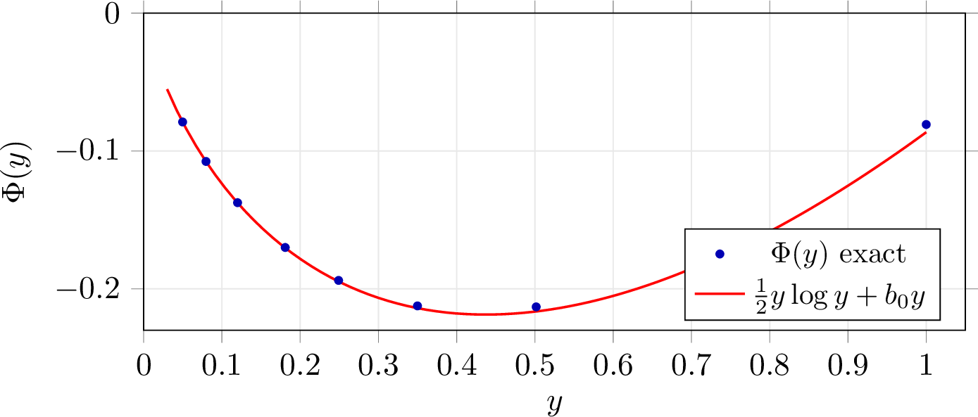
Numerical reliability was monitored in three ways: (i) comparison of the two representations of \(\Phi(y)\) (the scaled small-\(y\) representation and the \((\eta,\tau)\) representation for moderate and large \(y\)) in their overlap region; (ii) convergence with respect to the outer \(x=\log y\) grid; and (iii) stability of the finite-range fits. The production run used a uniform outer grid \(x\in[-17,8]\) with \(\Delta x=0.01\) (\(2501\) points). The \(\tau\) integral was evaluated with a 48-point Gauss–Laguerre rule, and the \(\eta\) integral used the grading \(\eta=\xi^2\) with a 10-point Gauss–Legendre rule on each panel. The same grid gives \(D_0^{\rm num}=0.2499026386\), while the exact value is \(D_0=0.2499018971\), a relative difference of \(2.97\times10^{-6}\). In the overlap check at \(y=0.03,0.05,0.1,0.2,0.3,0.5\), the maximum discrepancy \[\delta_\Phi=\frac{|\Phi_{\rm scaled}-\Phi_{\eta,\tau}|}{\max(1,|\Phi_{\rm scaled}|,|\Phi_{\eta,\tau}|)}\] was \(3.23\times10^{-4}\) and the root-mean-square value was \(1.77\times10^{-4}\). We additionally verified \(\int_0^\infty j_1(x)^2/x\,\mathrm{d}x=0.249999760\), \(\int_1^\infty u^{-2}L(u)\,\mathrm{d}u=1.386293781\), and \(\int_0^1\frac{\log(1/v)}{1-v^2}\,\mathrm{d}v=1.233699970\), consistent with \(\frac{1}{4}\), \(2\log2\), and \(\frac{\pi^2}{8}\), respectively.
7 Summary and outlook↩︎
The central point of this paper is that the contribution of one specific diagram—screened second-order exchange—can be reduced, for the separated Coulomb RC-SP model, to a one-dimensional integral, and that its dependence on the single-pole scale can then be studied from both asymptotic and numerical sides. First, we isolated the exact \(q\)–\(z\) multiplicative separability condition used by this reduction. Within the single-pole ansatz this condition selects a momentum-independent characteristic screening-frequency scale; it should not be read as a general impossibility theorem for every possible indirect representation of special nonseparable models. Second, we evaluated in closed form the static limit in which the screened line returns to the bare Coulomb interaction, and showed that its value coincides with the Onsager–Mittag–Stephen bare second-order exchange, thereby pinning the screening factor to an absolute energy scale. The numerical computation revealed a non-monotone intermediate maximum \(S(1)\simeq2.334\). Third, by the Mellin–Barnes method we obtained, with remainder estimates, the linear term in the small-\(\Lambda\) limit, the logarithmically corrected inverse-power law in the large-\(\Lambda\) limit, and the second small-\(\Lambda\) asymptotic term (\(\Lambda^2(\log\Lambda)^2\)).
7.1 Mapping to functional forms in \(r_s\)↩︎
If the single-pole scale \(\Lambda\) is mapped to the density parameter \(r_s\) by a power law \(\Lambda_{\mathrm{loc}}(r_s)=C_\Lambda r_s^{-\alpha}\), then the asymptotic forms in \(\Lambda\) obtained in the previous section, \[\{\Lambda^{-1}\log\Lambda,\;\Lambda^{-1},\;\Lambda,\;\Lambda^2(\log\Lambda)^2,\;\Lambda^2\log\Lambda,\;\Lambda^2\},\] translate into the linear span of the following functional forms in \(r_s\), \[\{r_s^{\alpha}\log r_s,\;r_s^{\alpha},\;r_s^{-\alpha},\;r_s^{-2\alpha}(\log r_s)^2,\;r_s^{-2\alpha}\log r_s,\;r_s^{-2\alpha}\}.\] What this paper provides is not a first-principles prediction of the exponent \(\alpha\), but a constrained family of functional forms suggested by the structure of the diagram; these can be used in place of empirically choosing a functional form for the residual correction of screened exchange.
7.2 Implication for the adiabatic-connection integral↩︎
The screened-second-order-exchange contribution studied here is one ingredient of the adiabatic-connection fluctuation–dissipation (ACFD) expression for the correlation energy [11], [14], in which a coupling constant \(\lambda\) is integrated from \(0\) to \(1\). Two features of our results bear on that integral without our having to carry it out.
First, the screening factor supplies exact constraints on the integrand. Since \(\tilde{\varepsilon}_{c,\mathrm{RC\text{-}SP}}(\infty)\) coincides with the Onsager–Mittag–Stephen bare second-order exchange 12 , the value \(S(\Lambda)\to1\) as \(\Lambda\to\infty\) is a closed-form reference point that any implementation of dynamically screened exchange must reproduce in the limit where the screened line becomes the bare Coulomb interaction; the endpoint asymptotics \(S(\Lambda)\sim A\Lambda\) (\(\Lambda\to0\)) and \(S(\Lambda)=1+(C_1\log\Lambda+C_0)/\Lambda+\cdots\) (\(\Lambda\to\infty\)) bound the integrand in the small-\(\Lambda\) and large-\(\Lambda\) regimes.
Second, the coupling dependence of the screening scale is not free but tied to its density dependence by coordinate scaling. The coupling-constant and coordinate-scaling formulations of the adiabatic connection are related by \(E_c^{\lambda}(r_s)=\lambda^{2}E_c(\lambda r_s)\) [20], [21]: the correlation energy at coupling \(\lambda\) and density \(r_s\) equals \(\lambda^{2}\) times the full-coupling correlation energy at the scaled density \(\lambda r_s\). If the screening scale tracks the local density as \(\Lambda_{\mathrm{loc}}(r_s)=C_\Lambda r_s^{-\alpha}\) (Sec. 7.1), the screening seen along the adiabatic connection at fixed \(r_s\) is therefore \(\Lambda(\lambda)=\lambda^{-\alpha}\Lambda(1)\), the screening of the scaled system at density \(\lambda r_s\). The same functional forms in \(r_s\) that are suggested by the diagram then also constrain the coupling-constant dependence of its contribution. In this scaling picture, the \(\lambda\to0\) vanishing expected of a correlation term is carried by the explicit prefactor \(\lambda^{2}\) rather than by \(S\) itself. We emphasize that this is a constraint on the analytic structure of the integrand—obtained from an exact scaling identity together with the modeling map of Sec. 7.1—and not an evaluation of the ACFD correlation energy itself: RC-SP is a controllable reference model, not a self-consistent account of how the physical screening evolves with \(\lambda\).
7.3 Outlook↩︎
There are three directions for future work. First, the RC-SP model can be studied as an auxiliary reference problem for dynamically screened exchange. As shown in Appendix 9, the Coulomb RC-SP kernel admits a formal Hubbard–Stratonovich representation as an interacting Fermi system with a retarded density–density interaction, or equivalently as a fermion–boson model in which a gapless bosonic field with linear dispersion \(\omega_{\boldsymbol{q}}=\Lambda|\boldsymbol{q}|\) couples to the electron density. This observation is meant only as a reference-model interpretation: it does not imply that the interaction is realized in an ordinary material, nor does it by itself remove the fermion sign problem. If a sign-free or mild-sign-problem lattice regularization can be found, quantum Monte Carlo calculations for this auxiliary model could provide useful benchmark data as a function of the single-pole scale \(\Lambda\). This possibility is only a future numerical test of the reference model; such data would complement, rather than replace, the usual UEG reference data used in LDA construction.
The second direction is the extension to a general pole model. The RC-SP kernel functions form a uniformly controlled single-pole family in the \(z\) direction on a \(\log\Lambda\) grid (\(|w_{\Lambda_1}-w_{\Lambda_2}|\le\frac{1}{2}|\log\Lambda_1-\log\Lambda_2|\)). If the radial direction is approximated by a rational function of \(q^2\) of Yukawa type, smooth corrections can be added while preserving the logarithmic singularity class \(\log|s_2/s_1|\) of the Coulomb case. A naive integer-power expansion is less suitable in the present coordinates, because it generates non-integrable ordinary-function singularities of type \(|R_k|^{-n}\). If the remaining part decays sufficiently fast at the endpoints, the leading Mellin poles are controlled by the finite-rank part, and the analysis of \(\Phi^{\mathrm{corr}}_0\), \(K_\Lambda\) and \(\Xi\) in this paper can be used as a starting point for more general separable approximations. If such approximations can be controlled, the single-pole result would provide a constraint on possible analytic forms of the screened exchange correction for broader classes of dynamic screening.
Third, the screening factor may serve as an input to coupling-constant modeling. If, in contrast to the scaling-fixed map of Sec. 7.2, the screening scale is assumed to track the coupling through the interaction strength itself, for instance \(\Lambda(\lambda)=\sqrt{\lambda}\,\Lambda(1)\) as suggested by the \(f\)-sum-rule scaling of a plasmon frequency, then a schematic contribution of the form \(\int_0^1\mathrm{d}\lambda\,\lambda S(\Lambda(\lambda))\) has a controlled small-\(\lambda\) endpoint: \(S(\Lambda)\sim A\Lambda\) gives an integrand of order \(\lambda^{3/2}\). This argument is only indicative, because the appropriate coupling dependence of the single scale \(\Lambda\) is not fixed by the present model. A first-principles determination of \(\Lambda(\lambda)\) is needed before this route can be promoted from a useful constraint to a predictive functional form.
Acknowledgments↩︎
No funding or other support was received. The author acknowledges the use of AI-based assistants—Claude (Claude Opus 4.8, Anthropic) and GPT-5.5 (OpenAI)—as interactive aids for exploring analytic manipulations during this work. All mathematical derivations and results were independently verified by the author, who takes full responsibility for the content.
8 Closed form of the static geometric factor \(D_0\)↩︎
We prove Proposition 1 of the main text (the closed form of the static geometric factor, \(D_0=-\tfrac\pi6G(3)\)). Applying the Weber–Schafheitlin-type formula \(\int_0^\infty j_1(ay)j_1(by)\,\mathrm{d}y=\frac{\pi b}{6a^2}\) (\(a\ge b>0\)) with \(a=\tfrac{u+v}2\ge b=\tfrac{u-v}2\), and using \(\frac{b}{a^2}=\frac{2(u-v)}{(u+v)^2}\), gives \[D_0=\frac{\pi}{3}\int_1^\infty\!\mathrm{d}u\,L(u)\,h(u),\qquad h(u)=\int_0^1\frac{u-v}{(u+v)^2}\log\frac{1}{uv}\,\mathrm{d}v. \label{eq:D0app}\tag{28}\] The inner integral closes elementarily. From \(\frac{u-v}{(u+v)^2}=\frac{2u}{(u+v)^2}-\frac{1}{u+v}\) and \(\int_0^1\frac{\log v}{(u+v)^2}\mathrm{d}v=-\frac{1}{u}\log\frac{u+1}{u}\), \(\int_0^1\frac{\log v}{u+v}\mathrm{d}v=\mathop{\mathrm{Li}}_2(-1/u)\), \[h(u)=-\frac{2\log u}{u+1}+\log u\,\log\frac{u+1}{u}+2\log\frac{u+1}{u}+\mathop{\mathrm{Li}}_2\!\Big(-\frac{1}{u}\Big). \label{eq:J0}\tag{29}\] The remaining outer integral \(g_0:=\int_1^\infty L(u)h(u)\mathrm{d}u\) is moved to the unit interval by \(u=1/x\) (\(x\in(0,1)\), \(\mathrm{d}u=-\mathrm{d}x/x^2\), \(L=\log\frac{1+x}{1-x}\)): \[\begin{gather} g_0=\int_0^1\frac{\mathrm{d}x}{x^2}\log\frac{1+x}{1-x}\,B(x),\\ B(x)=\underbrace{\frac{2x\log x}{1+x}}_{B_1}+\underbrace{\big[{-}\log x\log(1+x)+2\log(1+x)+\mathop{\mathrm{Li}}_2(-x)\big]}_{C(x)}. \end{gather} \label{eq:weight3}\tag{30}\] This integral is handled by logarithmic and polylogarithmic reductions; we split it as \(g_0=g_0^{(1)}+g_0^{(C)}\). In what follows we use the series \(\sum_{n\ge0}(2n+1)^{-3}=\frac{7}{8}\zeta(3)\), \(\mathop{\mathrm{Li}}_3(-1)=-\frac{3}{4}\zeta(3)\), and the following unit-interval logarithmic integrals. These identities are classical [22], but Lemma 6 derives them self-containedly from elementary functions and standard polylogarithm values only.
Lemma 6 (Logarithmic integrals on the unit interval). \[\begin{align} &\int_0^1\frac{\log x\log(1+x)}{x}\mathrm{d}x=-\frac{3}{4}\zeta(3), &&\int_0^1\frac{\log x\log(1+x)}{1+x}\mathrm{d}x=-\frac{1}{8}\zeta(3),\tag{31}\\ &\int_0^1\frac{\log x\log(1-x)}{1+x}\mathrm{d}x=\frac{13}{8}\zeta(3)-\frac{\pi^2}{4}\log2, &&\int_0^1\frac{\log^2(1+x)}{x}\mathrm{d}x=\frac{1}{4}\zeta(3),\tag{32}\\ &\int_0^1\frac{\log(1-x)\log(1+x)}{x}\mathrm{d}x=-\frac{5}{8}\zeta(3), &&\int_0^1\frac{\log x\log(1+x)}{1-x}\mathrm{d}x=\zeta(3)-\frac{\pi^2}{4}\log2.\tag{33} \end{align}\]
Proof. We use only the standard values \[\begin{gather} \eta(3):=\sum_{k\ge1}(-1)^{k-1}k^{-3}=\tfrac34\zeta(3),\quad \mathop{\mathrm{Li}}_3(-1)=-\tfrac34\zeta(3),\quad \mathop{\mathrm{Li}}_2(1)=\tfrac{\pi^2}{6},\\ \mathop{\mathrm{Li}}_2(-1)=-\tfrac{\pi^2}{12},\quad \sum_{m\ge0}(2m+1)^{-3}=\tfrac78\zeta(3), \end{gather}\] and the elementary formula \(\int_0^1 x^{k-1}\log x\,\mathrm{d}x=-k^{-2}\). We label the six integrals \(S_1,\dots,S_6\) in the order 31 –33 .
(i) Seed integrals. From \(\log(1\mp x)/x=\mp\sum_{k\ge1}(\pm1)^{k-1}x^{k-1}/k\), \[\sigma_0:=\int_0^1\frac{\log x\log(1-x)}{x}\mathrm{d}x=\zeta(3),\qquad S_1=\int_0^1\frac{\log x\log(1+x)}{x}\mathrm{d}x=-\eta(3)=-\frac{3}{4}\zeta(3).\]
(ii) Anchor \(I_0\). Integrating \(I_0:=\int_0^1\log^2(1-x)\,x^{-1}\mathrm{d}x\) by parts with \(\mathrm{d}(\log x)=x^{-1}\mathrm{d}x\) (boundary terms vanish) gives \(I_0=2\int_0^1\frac{\log x\log(1-x)}{1-x}\mathrm{d}x\), and \(x\mapsto1-x\) gives \(I_0=2\sigma_0=2\zeta(3)\).
(iii) \(S_5\). Use the identity \(\log(1-x)\log(1+x)=\frac{1}{4}\big[\log^2(1-x^2)-\log^2\tfrac{1+x}{1-x}\big]\). The first term, with \(w=x^2\), gives \(\int_0^1\log^2(1-x^2)\,x^{-1}\mathrm{d}x=\frac{1}{2} I_0=\zeta(3)\); the second, with \(t=\tfrac{1-x}{1+x}\) (\(\tfrac{1+x}{1-x}=t^{-1}\), \(\mathrm{d}x/x=-2\,\mathrm{d}t/(1-t^2)\)), \[\int_0^1\frac{1}{x}\log^2\frac{1+x}{1-x}\mathrm{d}x=2\int_0^1\frac{\log^2 t}{1-t^2}\mathrm{d}t=4\sum_{m\ge0}\frac{1}{(2m+1)^3}=\frac{7}{2}\zeta(3).\] Hence \(S_5=\frac{1}{4}\big(\zeta(3)-\frac{7}{2}\zeta(3)\big)=-\frac{5}{8}\zeta(3)\).
(iv) \(S_4\) and \(S_2\). From the Cauchy product \(\log^2(1+x)=2\sum_{n\ge1}(-1)^n H_{n-1}\,x^n/n\) (\(H_n\) the harmonic number, \(H_0=0\)). Integrating term by term and using \(H_{n-1}=H_n-1/n\) gives \(S_4=2\sum_{n\ge1}(-1)^n H_n/n^2-2\mathop{\mathrm{Li}}_3(-1)\). Here, from \(H_n/n=-\int_0^1 x^{n-1}\log(1-x)\mathrm{d}x\) and \(\sum_{n\ge1}(-1)^n x^{n-1}/n=-x^{-1}\log(1+x)\), \[\sum_{n\ge1}(-1)^n\frac{H_n}{n^2}=-\int_0^1\log(1-x)\sum_{n\ge1}\frac{(-1)^n x^{n-1}}{n}\,\mathrm{d}x =\int_0^1\frac{\log(1-x)\log(1+x)}{x}\mathrm{d}x=S_5,\] hence \(S_4=2S_5-2\mathop{\mathrm{Li}}_3(-1)=2\big(-\frac{5}{8}+\frac{3}{4}\big)\zeta(3)=\frac{1}{4}\zeta(3)\). Also, integrating \(\frac{\log(1+x)}{1+x}=\frac{\mathrm{d}}{\mathrm{d}x}\frac{1}{2}\log^2(1+x)\) by parts (boundary terms vanish) gives \(S_2=-\frac{1}{2} S_4=-\frac{1}{8}\zeta(3)\).
(v) \(S_3\). From the Cauchy product \(\frac{\log(1-x)}{1+x}=\sum_{n\ge1}(-1)^n\overline{H}_n\,x^n\), \(\overline{H}_n=\sum_{k=1}^n(-1)^{k-1}/k\). Integrating term by term (\(\int_0^1 x^n\log x\,\mathrm{d}x=-(n+1)^{-2}\), \(n\to m-1\)) and using \(\overline{H}_{m-1}=\overline{H}_m+(-1)^m/m\) gives \(S_3=\sum_{m\ge1}(-1)^m\overline{H}_{m-1}/m^2=W+\zeta(3)\), \(W:=\sum_{m\ge1}(-1)^m\overline{H}_m/m^2\). From \(\overline{H}_m=\int_0^1\frac{1-(-x)^m}{1+x}\mathrm{d}x\), \[W=\int_0^1\frac{\mathop{\mathrm{Li}}_2(-1)-\mathop{\mathrm{Li}}_2(x)}{1+x}\mathrm{d}x=\mathop{\mathrm{Li}}_2(-1)\log2-\int_0^1\frac{\mathop{\mathrm{Li}}_2(x)}{1+x}\mathrm{d}x,\] where the last integral, by integrating \(\mathop{\mathrm{Li}}_2'(x)=-\log(1-x)/x\) by parts, equals \(\mathop{\mathrm{Li}}_2(1)\log2+S_5=\frac{\pi^2}{6}\log2-\frac{5}{8}\zeta(3)\). Hence \(W=-\frac{\pi^2}{12}\log2-\big(\frac{\pi^2}{6}\log2-\frac{5}{8}\zeta(3)\big)=\frac{5}{8}\zeta(3)-\frac{\pi^2}{4}\log2\), i.e. \(S_3=\frac{13}{8}\zeta(3)-\frac{\pi^2}{4}\log2\).
(vi) \(S_6\). Integrating by parts with \(\mathrm{d}(-\log(1-x))=\mathrm{d}x/(1-x)\) (boundary terms vanish), \[\begin{align} S_6=\int_0^1\log(1-x)\,\mathrm{d}\big[\log x\log(1+x)\big] &=\int_0^1\frac{\log(1-x)\log(1+x)}{x}\mathrm{d}x+\int_0^1\frac{\log x\log(1-x)}{1+x}\mathrm{d}x\\ &=S_5+S_3=\zeta(3)-\frac{\pi^2}{4}\log2. \end{align}\] All six values are rational-coefficient combinations of \(\zeta(3)\) and \(\pi^2\log2\); since the arguments are restricted to the reals \(x,1\pm x\), no additional constants such as Catalan’s constant appear. ◻
We now evaluate the first part \(g_0^{(1)}\). From \(\frac{1}{x(1+x)}=\frac{1}{x}-\frac{1}{1+x}\), \[\begin{gather} g_0^{(1)}=\int_0^1\frac{2\log x}{x(1+x)}\log\frac{1+x}{1-x}\mathrm{d}x=2(K_1-K_2),\\ K_1=\int_0^1\frac{\log x}{x}\log\frac{1+x}{1-x}\mathrm{d}x,\qquad K_2=\int_0^1\frac{\log x}{1+x}\log\frac{1+x}{1-x}\mathrm{d}x. \end{gather}\] From \(\log\frac{1+x}{1-x}=2\sum_{n\ge0}\frac{x^{2n+1}}{2n+1}\) and \(\int_0^1 x^{2n}\log x\,\mathrm{d}x=-(2n+1)^{-2}\), \(K_1=-2\sum_{n\ge0}(2n+1)^{-3}=-\frac{7}{4}\zeta(3)\). Also, from \(\log\frac{1+x}{1-x}=\log(1+x)-\log(1-x)\) and 31 ,32 , \(K_2=-\frac{1}{8}\zeta(3)-\big(\frac{13}{8}\zeta(3)-\frac{\pi^2}{4}\log2\big)=-\frac{7}{4}\zeta(3)+\frac{\pi^2}{4}\log2\). Hence \(\zeta(3)\) cancels and \[g_0^{(1)}=2(K_1-K_2)=-\frac{\pi^2}{2}\log2. \label{eq:g01}\tag{34}\]
We now evaluate the second part \(g_0^{(C)}\). Set \(g(x):=\log x\log(1+x)-\mathop{\mathrm{Li}}_2(-x)\), \(\Psi(x):=g(x)/x\). Then \(C(x)=-g(x)+2\log(1+x)\), and from \(g'(x)=\frac{2\log(1+x)}{x}+\frac{\log x}{1+x}\), \(\Psi'=\frac{g'}{x}-\frac{g}{x^2}\), the following key identity follows: \[\frac{C(x)}{x^2}=-\frac{g}{x^2}+\frac{2\log(1+x)}{x^2} =\frac{\mathrm{d}}{\mathrm{d}x}\Psi(x)-\frac{\log x}{x(1+x)}. \label{eq:keyid}\tag{35}\] This recasting into \(\Psi'\) is the key device that makes every integration by parts close on the finite list of logarithmic integrals 31 –33 . Evaluating \(C(x)/x^2\) term by term, the individual pieces contain lower-order endpoint terms (for instance \(\int_0^1\log(1+x)\log(1-x)\,x^{-2}\mathrm{d}x=-\log^2 2-\frac{\pi^2}{12}\)) that cancel to leave the final combination; the assembly into \(\Psi'\) avoids this mixing of endpoint-singular pieces and the cancellation of endpoint divergences. Note that the integrands involve only the real arguments \(-x,\,1\pm x\), so the constants that appear reduce to combinations of \(\zeta(3)\), \(\pi^2\log2\), \(\log^3 2\) and lower-order logarithmic constants; no additional constant such as Catalan’s constant appears. Using this (the \(1/x^2\) drops out), \[g_0^{(C)}=\int_0^1\frac{C(x)}{x^2}\log\frac{1+x}{1-x}\mathrm{d}x =\underbrace{\int_0^1\Psi'(x)\log\frac{1+x}{1-x}\mathrm{d}x}_{=:T} -\underbrace{\int_0^1\frac{\log x}{x(1+x)}\log\frac{1+x}{1-x}\mathrm{d}x}_{=\,\frac{1}{2} g_0^{(1)}=-\frac{\pi^2}{4}\log2}.\] Split \(T\) via \(\log\frac{1+x}{1-x}=\log(1+x)-\log(1-x)\) and integrate each by parts. From \(\Psi(1)=g(1)=-\mathop{\mathrm{Li}}_2(-1)=\frac{\pi^2}{12}\) and the vanishing at the endpoints (\(\Psi(x)\sim\log x+1\) as \(x\downarrow0\), \(\log(1\pm x)\sim\pm x\)), \[\begin{align} T_+&=\int_0^1\Psi'\log(1+x)\mathrm{d}x=\frac{\pi^2}{12}\log2-\int_0^1\frac{\Psi(x)}{1+x}\mathrm{d}x,\\ T_-&=\int_0^1\Psi'\log(1-x)\mathrm{d}x =\Big[(\Psi-\Psi(1))\log(1-x)\Big]_0^1+\int_0^1\frac{\Psi(x)-\Psi(1)}{1-x}\mathrm{d}x\notag\\ &=\int_0^1\frac{\Psi(x)-\Psi(1)}{1-x}\mathrm{d}x=:R, \end{align}\] where the boundary term of \(T_-\) vanishes because \(\Psi-\Psi(1)=O(1-x)\). The first integral, via \(\frac{1}{x(1+x)}=\frac{1}{x}-\frac{1}{1+x}\), \(\int_0^1\frac{g}{x}\mathrm{d}x=\int_0^1\frac{\log x\log(1+x)}{x}\mathrm{d}x-\mathop{\mathrm{Li}}_3(-1)=-\frac{3}{4}\zeta(3)+\frac{3}{4}\zeta(3)=0\), and \(\int_0^1\frac{\mathop{\mathrm{Li}}_2(-x)}{1+x}\mathrm{d}x=\big[\log(1+x)\mathop{\mathrm{Li}}_2(-x)\big]_0^1+\int_0^1\frac{\log^2(1+x)}{x}\mathrm{d}x=-\frac{\pi^2}{12}\log2+\frac{1}{4}\zeta(3)\) (using the right entry of 32 ), gives \[\int_0^1\frac{\Psi}{1+x}\mathrm{d}x=\int_0^1\frac{g}{x}\mathrm{d}x-\int_0^1\frac{g}{1+x}\mathrm{d}x =0-\Big[{-}\tfrac18\zeta(3)-\big(\tfrac14\zeta(3)-\tfrac{\pi^2}{12}\log2\big)\Big] =\frac{3}{8}\zeta(3)-\frac{\pi^2}{12}\log2.\] By \(\frac{1}{x(1-x)}=\frac{1}{x}+\frac{1}{1-x}\) and \(\int_0^1\frac{g}{x}=0\), \(R\) reduces to \(R=\int_0^1\frac{g(x)-g(1)}{1-x}\mathrm{d}x\), and from \(g(1)=\frac{\pi^2}{12}=-\mathop{\mathrm{Li}}_2(-1)\) and \(\log x\log(1+x)|_{x=1}=0\) we have \(g(x)-g(1)=\log x\log(1+x)-[\mathop{\mathrm{Li}}_2(-x)-\mathop{\mathrm{Li}}_2(-1)]\), hence \[R=\int_0^1\frac{\log x\log(1+x)}{1-x}\mathrm{d}x-\int_0^1\frac{\mathop{\mathrm{Li}}_2(-x)-\mathop{\mathrm{Li}}_2(-1)}{1-x}\mathrm{d}x=R_1-R_2.\] Here \(R_1=\zeta(3)-\frac{\pi^2}{4}\log2\) (right entry of 33 ). \(R_2\), by integration by parts (\(v=-\log(1-x)\), \(\frac{\mathrm{d}}{\mathrm{d}x}[\mathop{\mathrm{Li}}_2(-x)-\mathop{\mathrm{Li}}_2(-1)]=-\frac{\log(1+x)}{x}\), boundary terms vanish), equals \(R_2=-\int_0^1\frac{\log(1-x)\log(1+x)}{x}\mathrm{d}x=\frac{5}{8}\zeta(3)\) (left entry of 33 ). Hence \(R=\big(\zeta(3)-\frac{\pi^2}{4}\log2\big)-\frac{5}{8}\zeta(3)=\frac{3}{8}\zeta(3)-\frac{\pi^2}{4}\log2\). Combining, \[T=\frac{\pi^2}{12}\log2-\Big(\frac{3}{8}\zeta(3)-\frac{\pi^2}{12}\log2\Big)-\Big(\frac{3}{8}\zeta(3)-\frac{\pi^2}{4}\log2\Big) =\frac{5\pi^2}{12}\log2-\frac{3}{4}\zeta(3),\] \[g_0^{(C)}=T+\frac{\pi^2}{4}\log2=\frac{2\pi^2}{3}\log2-\frac{3}{4}\zeta(3). \label{eq:g0C}\tag{36}\]
Composing both parts, 34 and 36 give \[g_0=g_0^{(1)}+g_0^{(C)}=-\frac{\pi^2}{2}\log2+\frac{2\pi^2}{3}\log2-\frac{3}{4}\zeta(3)=\frac{\pi^2}{6}\log2-\frac{3}{4}\zeta(3),\] hence \[D_0=\frac{\pi}{3}g_0=\frac{\pi^{3}}{18}\log2-\frac{\pi}{4}\zeta(3)=-\frac{\pi}{6}G(3),\qquad G(3)=\frac{3}{2}\zeta(3)-\frac{\pi^2}{3}\log2, \label{eq:D0final}\tag{37}\] which is Proposition 1. This derivation does not rely on Glasser’s evaluation, and because Lemma 6 derives the required logarithmic integrals internally, it is self-contained and does not depend on external integral tables either. As an independent check, regularizing 30 via the \(\mathop{\mathrm{Li}}_2\) representation 29 with \(u=(1+t)/(1-t)\) (\(L=-\log t\)) and performing high-precision quadrature agrees with 37 to \(60\) digits, and the integer relation \(12\,g_0+9\zeta(3)-2\pi^2\log2=0\) holds. Furthermore, the result is consistent with Glasser’s \(d=3\) value[16] through \(G(3)/(\tfrac3\pi D_0)=-2\).
9 Time-ordered transfer kernel and auxiliary fermion–boson representation↩︎
This appendix gives a compact zero-temperature formulation that parallels the Matsubara definition used in the main text. Its purpose is limited: it shows that, after the internal fermionic frequency is integrated out, the same off-axis transfer kernel appears. It does not assert an identity between the finite-temperature grand-potential construction and a completed ground-state correlation functional.
We normalize \(k_F=1\) and write \[\xi_{\boldsymbol{p}}:=\varepsilon_{\boldsymbol{p}}-\varepsilon_F .\] The zero-temperature time-ordered one-particle propagator is \[G^F_0(\boldsymbol{p},\omega)= \frac{\Theta(|\boldsymbol{p}|-1)}{\omega-\xi_{\boldsymbol{p}}+\mathrm{i}0} +\frac{\Theta(1-|\boldsymbol{p}|)}{\omega-\xi_{\boldsymbol{p}}-\mathrm{i}0}.\] For a fixed transfer \((\boldsymbol{q},\omega)\), the internal fermionic frequency integral of one particle–hole block gives \[Q^T_0(\boldsymbol{p};\boldsymbol{q},\omega)= \frac{\Delta(\boldsymbol{p};\boldsymbol{q})}{\omega-\delta(\boldsymbol{p};\boldsymbol{q})+\mathrm{i}0\,\operatorname{sgn}\Delta(\boldsymbol{p};\boldsymbol{q})}, \qquad \delta(\boldsymbol{p};\boldsymbol{q})=\xi_{\boldsymbol{p}+\boldsymbol{q}}-\xi_{\boldsymbol{p}}=\boldsymbol{p}\cdot\boldsymbol{q}+\frac{q^2}{2}.\] Equivalently, away from the real transfer-frequency axis we introduce \[Q^\sharp_0(\boldsymbol{p};\boldsymbol{q},z):=\frac{\Delta(\boldsymbol{p};\boldsymbol{q})}{z-\delta(\boldsymbol{p};\boldsymbol{q})}, \qquad z\in\mathbb{C}\setminus\mathbb{R},\] with the off-axis transfer kernel \[X^\sharp(\boldsymbol{q},z)=\int \mathrm{d}^3p\,\mathrm{d}^3k\, \frac{1}{|\boldsymbol{p}-\boldsymbol{k}|^2} Q^\sharp_0(\boldsymbol{p};\boldsymbol{q},z)Q^\sharp_0(\boldsymbol{k};\boldsymbol{q},z).\] On the imaginary axis this becomes \[X^\sharp(\boldsymbol{q},\mathrm{i}\xi)=\int \mathrm{d}^3p\,\mathrm{d}^3k\, \frac{1}{|\boldsymbol{p}-\boldsymbol{k}|^2} \frac{\Delta(\boldsymbol{p};\boldsymbol{q})\Delta(\boldsymbol{k};\boldsymbol{q})}{[\mathrm{i}\xi-\delta(\boldsymbol{p};\boldsymbol{q})][\mathrm{i}\xi-\delta(\boldsymbol{k};\boldsymbol{q})]},\] which is the kernel \(X(\boldsymbol{q},\xi)\) used in Eq. 5 . If the screened interaction has an off-axis continuation \(D^\sharp(\boldsymbol{q},z)\) whose product with \(X^\sharp(\boldsymbol{q},z)\) is analytic away from the real axis and decays sufficiently on large semicircles, the transfer-frequency contour can be deformed to the imaginary axis. Under these standard analytic-continuation assumptions one recovers \[I^{(0)}_{\mathrm{scr2x}}[D]=A_0\int_0^\infty\frac{\mathrm{d}\xi}{\pi}\int \mathrm{d}^3q\, D(\boldsymbol{q},\mathrm{i}\xi)X(\boldsymbol{q},\xi),\] which has the same algebraic form as the main-text model quantity.
For the Coulomb RC-SP kernel one may choose the off-axis bosonic continuation \[D^\sharp_{\Lambda}(\boldsymbol{q},z)=\frac{\Lambda^2}{-z^2+\Lambda^2q^2}, \qquad D^\sharp_{\Lambda}(\boldsymbol{q},\mathrm{i}\xi)=\frac{\Lambda^2}{\xi^2+\Lambda^2q^2}.\] Thus the \(\xi=qz\) reduction of the main text applies line by line.
The same kernel also has a formal Hubbard–Stratonovich representation. Consider the Euclidean retarded density–density interaction \[V_\Lambda(\boldsymbol{q},\mathrm{i}\xi_m):=g\, \frac{\Lambda^2}{\xi_m^2+\Lambda^2q^2},\qquad g>0.\] For the fermionic density \(\rho_{\boldsymbol{q},m}:=\sum_{\boldsymbol{k},n,\sigma}\bar\psi_{\boldsymbol{k}+\boldsymbol{q},n+m,\sigma}\psi_{\boldsymbol{k},n,\sigma}\), a Gaussian Hubbard–Stratonovich transformation gives, formally, \[\begin{align} &\exp\!\left[-\frac{1}{2\beta V}\sum_{\boldsymbol{q},m} \rho_{-\boldsymbol{q},-m}V_\Lambda(\boldsymbol{q},\mathrm{i}\xi_m)\rho_{\boldsymbol{q},m}\right] \\ &\qquad \propto \int\mathcal{D}\varphi\, \exp\!\left[-\frac{1}{2\beta V}\sum_{\boldsymbol{q},m} \varphi_{-\boldsymbol{q},-m}V_\Lambda^{-1}\varphi_{\boldsymbol{q},m} +\frac{\mathrm{i}}{\beta V}\sum_{\boldsymbol{q},m}\varphi_{-\boldsymbol{q},-m}\rho_{\boldsymbol{q},m}\right]. \end{align}\] Since \[V_\Lambda(\boldsymbol{q},\mathrm{i}\xi_m)^{-1}=\frac{\xi_m^2+\Lambda^2q^2}{g\Lambda^2},\] rescaling \(\varphi=\sqrt g\,\Lambda\,\phi\) yields the auxiliary fermion–boson action \[\begin{align} S[\bar\psi,\psi,\phi] &=\sum_{\boldsymbol{k},n,\sigma}\bar\psi_{\boldsymbol{k}n\sigma}(-\mathrm{i}\omega_n+\xi_{\boldsymbol{k}})\psi_{\boldsymbol{k}n\sigma} +\frac{1}{2\beta V}\sum_{\boldsymbol{q},m}\phi_{-\boldsymbol{q},-m}(\xi_m^2+\Lambda^2q^2)\phi_{\boldsymbol{q},m} \\ &\quad -\frac{\mathrm{i}\sqrt g\,\Lambda}{\beta V}\sum_{\boldsymbol{q},m}\phi_{-\boldsymbol{q},-m}\rho_{\boldsymbol{q},m} . \end{align}\] In coordinate space, the bosonic quadratic part is \[S_b[\phi]=\frac{1}{2}\int_0^\beta\mathrm{d}\tau\int\mathrm{d}^3x\, \big[(\partial_\tau\phi)^2+\Lambda^2(\nabla\phi)^2\big],\] so the auxiliary boson has the linear dispersion \(\omega_{\boldsymbol{q}}=\Lambda|\boldsymbol{q}|\). This representation is useful as a possible reference problem, but the imaginary coupling means that a sign problem can remain; any quantum Monte Carlo application would need a regularization in which that issue is absent or quantitatively controlled.
10 Numerical algorithm↩︎
The quantities to be evaluated are the geometric block \(\Phi(y)\) of the main text and \(S(\Lambda)=N(\Lambda)/D_0\), \(N(\Lambda)=\int_0^\infty\frac{\Phi(y)}{y}\Xi(\Lambda y)\mathrm{d}y\), \(D_0=\int_0^\infty\frac{\Phi(y)}{y}\mathrm{d}y\). We use the series \(j_1(z)=\frac{z}{3}-\frac{z^3}{30}+\cdots\) for \(j_1\) at small argument, the finite-interval representation \(\Xi(z)=z\int_0^{\pi/2}\mathrm{e}^{-z\tan\theta}\mathrm{d}\theta\) as one exact representation for \(\Xi\). In the verification code used for the present manuscript, we use the equivalent closed form in terms of \(\mathop{\mathrm{Si}}\) and \(\mathop{\mathrm{Ci}}\), together with the small- and large-\(z\) asymptotics (\(\Xi(z)=\frac{\pi}{2} z+z^2(\log z+\gamma-1)+\cdots\), \(\Xi(z)=1-2z^{-2}+24z^{-4}-\cdots\)) for stabilization.
The difficulty for \(\Phi(y)\) lies in the logarithmic singularity at \(u=1\), \(v=0\) and in the shift of the dominant contribution to \(u\sim y^{-1}\) at small \(y\). We use two representations according to the size of \(y\). For \(y\ll1\), set \(t=uy\), \(v=\mathrm{e}^{-\tau}\) and write \[\Phi(y)=\int_y^\infty\!\mathrm{d}t\,L(t/y)\int_0^\infty\!\mathrm{d}\tau\,\mathrm{e}^{-\tau}\big(\log(y/t)+\tau\big) j_1\!\Big(\tfrac{t+y\mathrm{e}^{-\tau}}2\Big)j_1\!\Big(\tfrac{t-y\mathrm{e}^{-\tau}}2\Big)\] to keep the dominant region at \(t=O(1)\). For moderate and large \(y\), with the endpoint-absorbing variables \(u=\cosh\eta\), \(v=\mathrm{e}^{-\tau}\), \[\Phi(y)=y\int_0^\infty\!\mathrm{d}\eta\,\sinh\eta\,L(\cosh\eta)\int_0^\infty\!\mathrm{d}\tau\,\mathrm{e}^{-\tau}\big(\tau-\log\cosh\eta\big) j_1\!\Big(\tfrac{\cosh\eta+\mathrm{e}^{-\tau}}2y\Big)j_1\!\Big(\tfrac{\cosh\eta-\mathrm{e}^{-\tau}}2y\Big)\] absorbs the endpoint singularity into an integrable weight on a half-infinite interval. The outer integral is taken with \(y=\mathrm{e}^x\) as \(D_0=\int_{-\infty}^\infty\Phi(\mathrm{e}^x)\mathrm{d}x\), \(N(\Lambda)=\int_{-\infty}^\infty\Phi(\mathrm{e}^x)\Xi(\Lambda\mathrm{e}^x)\mathrm{d}x\); \(\Phi(\mathrm{e}^x)\) is tabulated once on a uniform \(x\) grid, and \(D_0,N(\Lambda)\) are computed from the same table. Since numerator and denominator share the same table, interpolation errors tend to cancel. In the production calculation reported in Sec. 6, we used \(x\in[-17,8]\) with \(\Delta x=0.01\). The inner \(\tau\) integral used a 48-point Gauss–Laguerre rule. The \(\eta\) integral used the grading \(\eta=\xi^2\) and a composite 10-point Gauss–Legendre rule, with the cutoff \(\eta_{\max}=\max\{25,\log(4/y)+22\}\). The denominator of the final normalized factor was the exact closed-form value of \(D_0\), while the numerical value of the same integral was used as an independent check. At large \(\Lambda\) the weight of the integrand shifts to small \(y\) (\(y\sim\Lambda^{-1}\)), so a stable evaluation of \(\Phi\) in this region is the key point for the numerical verification of the coefficient \(C_1\).
11 Rigorous asymptotic analysis: overview and notation↩︎
Scope. These analytical appendices provide the rigorous analytic backbone for the asymptotic statements of the main text. The treatment is logically self-contained: starting from the reduced one-variable block \(\Phi\) and the screening kernel \(\Xi\) defined in the main text, we (i) establish the analytic properties of the kernel Mellin transform \(K(s)\) with full proofs (Appendix 13); (ii) justify the Mellin–Barnes representation of the normalized screening factor \(S(\Lambda)\) (Appendix 14); (iii) prove the general contour-shift theorem (Theorem 4) that converts the displacement of the integration line into a residue series with an explicit remainder bound, together with the residue-to-asymptotic rule (Appendix 15); (iv) carry out the endpoint analysis of \(\Phi\) that fixes the principal part of its Mellin transform \(F(s)\) at \(s=-1\) and \(s=2\) (Appendix 16); (v) control the vertical growth of the regular part \(H_2(s)\) on the closed strip \(0<\operatorname{Re}s<3\) (Appendix 17); and (vi) assemble these into large-\(\Lambda\) and small-\(\Lambda\) expansions with explicit remainder estimates, including the second small-\(\Lambda\) term \(\Lambda^2(\log\Lambda)^2\) (Appendix 18). A table of independent numerical cross-checks is collected in Appendix 19.
Notation. Throughout, \[\Phi(y):=y\int_1^\infty\!\mathrm{d}u\,L(u)\int_0^1\!\mathrm{d}v\,\ell(u,v)\, j_1\!\Big(\tfrac{u+v}{2}y\Big)\,j_1\!\Big(\tfrac{u-v}{2}y\Big), \quad L(u)=\log\frac{u+1}{u-1},\;\;\ell(u,v)=\log\frac{1}{uv}, \label{smeq:Phidef}\tag{38}\] where \(j_1(z)=\sin z/z^2-\cos z/z\) is the spherical Bessel function. We write \[F(s):=\int_0^\infty y^{s-1}\Phi(y)\,\mathrm{d}y,\qquad D_0:=\int_0^\infty\frac{\Phi(y)}{y}\,\mathrm{d}y=F(0),\] \[\Xi(z):=z\int_0^\infty\frac{\mathrm{e}^{-zt}}{1+t^2}\,\mathrm{d}t,\qquad K(s):=\mathcal{M}[\Xi](s)=\int_0^\infty z^{s-1}\Xi(z)\,\mathrm{d}z,\] and the normalized screening factor \[S(\Lambda):=\frac{1}{D_0}\int_0^\infty\frac{\Phi(y)}{y}\,\Xi(\Lambda y)\,\mathrm{d}y . \label{smeq:Sdef}\tag{39}\] We use the standard bounds \[\abs{j_1(z)}\le C\min\{z,(1+z)^{-1}\},\qquad \abs{j_1'(z)}\le C\min\{1,z^{-1}\}\quad(z>0), \label{smeq:j1bounds}\tag{40}\] \(\gamma\) denotes the Euler–Mascheroni constant, and for \(X\in L^1_{\mathrm{loc}}([1,\infty))\) we abbreviate \(\mathcal{M}_{>}[X](s):=\int_1^\infty y^{s-1}X(y)\,\mathrm{d}y\). The constant \(D_0=\tfrac{\pi^3}{18}\log2-\tfrac{\pi}{4}\zeta(3)=-\tfrac\pi6 G(3) =0.2499018971\ldots\) is the closed-form static factor established in Appendix 8.
12 The reduced block: preliminary facts↩︎
We record the two facts that frame the entire analysis; both are proved in Appendix 16.
Proposition 2 (A priori envelope). There is a constant \(C>0\) such that \[\abs{\Phi(y)}\le C\,y\,(1+\abs{\log y})\quad(0<y\le1),\qquad \abs{\Phi(y)}\le C\,y^{-2}(1+\log y)\quad(y\ge1). \label{smeq:envelope}\qquad{(1)}\] Consequently \(F(s)\) converges absolutely and is holomorphic on the strip \(-1<\operatorname{Re}s<2\), with \(D_0=F(0)\).
The exponents in ?? are sharp: \(\Phi\) carries a \(y\log y\) singularity as \(y\downarrow0\) (whence the double pole of \(F\) at \(s=-1\)) and a \(y^{-2}\) tail as \(y\to\infty\) (whence the simple pole of \(F\) at \(s=2\)). Fixing the coefficients of these singularities is the entire content of Appendix 16.
13 The screening kernel and its Mellin transform↩︎
The asymptotics of \(S(\Lambda)\) are governed by the meromorphic structure of \(K(s)\), which we now establish with complete proofs.
Lemma 7 (Closed form and Mellin transform of \(\Xi\)). For \(z>0\), \[\Xi(z)=z\Big[\mathop{\mathrm{Ci}}(z)\sin z+\big(\tfrac{\pi}{2}-\mathop{\mathrm{Si}}(z)\big)\cos z\Big], \label{smeq:Xiclosed}\tag{41}\] and the Mellin transform \[K(s)=-\frac{\pi}{2}\,\frac{\Gamma(s+1)}{\sin(\pi s/2)} \label{smeq:Ks}\tag{42}\] holds for \(-1<\operatorname{Re}s<0\); the right-hand side is the meromorphic continuation of \(K\) to all of \(\mathbb{C}\).
Proof. Write \(f(z):=\int_0^\infty \mathrm{e}^{-zt}/(1+t^2)\,\mathrm{d}t\), so \(\Xi=zf\). The exponential-integral representations of the sine and cosine integrals give the classical Laplace evaluation \(f(z)=\mathop{\mathrm{Ci}}(z)\sin z+(\tfrac\pi2-\mathop{\mathrm{Si}}(z))\cos z\), which is 41 . From 41 , \(\Xi(z)=O(z)\) as \(z\downarrow0\) and \(\Xi(z)=O(1)\) as \(z\to\infty\), so on \(-1<\operatorname{Re}s<0\) the integrand \(z^{s-1}\Xi(z)=z^s f(z)\) is absolutely integrable; moreover \(z^s\mathrm{e}^{-zt}(1+t^2)^{-1}\) is absolutely integrable on \((0,\infty)^2\) there, so Fubini gives \[K(s)=\int_0^\infty\frac{\mathrm{d}t}{1+t^2}\int_0^\infty z^{s}\mathrm{e}^{-zt}\,\mathrm{d}z =\Gamma(s+1)\int_0^\infty\frac{t^{-s-1}}{1+t^2}\,\mathrm{d}t .\] Substituting \(u=t^2\) and using \(\int_0^\infty u^{\alpha-1}(1+u)^{-1}\mathrm{d}u=\pi/\sin(\pi\alpha)\) (\(0<\operatorname{Re}\alpha<1\)) at \(\alpha=-s/2\), the \(t\)-integral equals \(-\tfrac{\pi}{2}\big/\sin(\pi s/2)\), yielding 42 . The right-hand side is meromorphic on \(\mathbb{C}\) and agrees with \(K\) on the strip, hence is its continuation. ◻
Lemma 8 (Functional equation). \(K(s+2)=-(s+1)(s+2)\,K(s)\) for all \(s\in\mathbb{C}\).
Proof. Immediate from 42 via \(\Gamma(s+3)=(s+1)(s+2)\Gamma(s+1)\) and \(\sin\!\big(\tfrac{\pi(s+2)}{2}\big)=-\sin\!\big(\tfrac{\pi s}{2}\big)\). It reflects, at the level of Mellin images, that \(\Xi=zf\) with \(f\) obeying the inhomogeneous ODE \(f''+f=1/z\). ◻
Lemma 9 (Poles, residues, and local expansions). \(K\) is meromorphic with poles only at the integers, and:
at \(s=2k\) \((k\ge0)\): a simple pole, \(\mathop{\mathrm{Res}}_{s=2k}K=(-1)^{k+1}(2k)!\);
at \(s=-(2k+1)\) \((k\ge0)\): a simple pole, \(\mathop{\mathrm{Res}}_{s=-(2k+1)}K=\tfrac{\pi}{2}(-1)^k/(2k)!\);
at \(s=-2k\) \((k\ge1)\): a double pole.
In particular \[K(s)=-\frac{1}{s}+\gamma+O(s)\;\;(s\to0),\qquad K(s)=-\frac{1}{(s+2)^2}+\frac{\gamma-1}{s+2}+O(1)\;\;(s\to-2), \label{smeq:Klaurent}\tag{43}\] and \(K(1)=-\tfrac\pi2\), \(K'(1)=-\tfrac\pi2(1-\gamma)\).
Proof. In 42 , \(\sin(\pi s/2)\) has simple zeros at the even integers and \(\Gamma(s+1)\) has simple poles at the negative integers. At a nonnegative even integer \(\Gamma\) is finite and nonzero, giving a simple pole of \(K\); at a negative odd integer \(\sin\neq0\), so the simple pole of \(\Gamma\) gives a simple pole of \(K\); at a negative even integer the simple pole of \(\Gamma\) coincides with the simple zero of \(\sin\), giving a double pole. For the residues, use \(\sin\!\big(\tfrac\pi2(2k+\varepsilon)\big)=(-1)^k\tfrac{\pi\varepsilon}{2}+O(\varepsilon^3)\) and \(\Gamma(2k+1)=(2k)!\) for (i). For (ii), \(\mathop{\mathrm{Res}}_{s=-(2k+1)}\Gamma(s+1)=1/(2k)!\) and \(\sin\!\big(\tfrac\pi2(-(2k+1))\big)=(-1)^{k+1}\); they satisfy the recursion \(\mathop{\mathrm{Res}}_{s=2k+2}K=-(2k+1)(2k+2)\mathop{\mathrm{Res}}_{s=2k}K\) forced by Lemma 8. The expansions 43 follow by inserting \(\Gamma(1+\varepsilon)=1-\gamma\varepsilon+O(\varepsilon^2)\) at \(s=\varepsilon\) and \(\Gamma(-1+\varepsilon)=-\varepsilon^{-1}+(\gamma-1)+O(\varepsilon)\), \(\sin\!\big(\tfrac\pi2(-2+\varepsilon)\big)=\tfrac{\pi\varepsilon}{2}+O(\varepsilon^3)\) at \(s=-2+\varepsilon\). Finally \(K(1)=-\tfrac\pi2\Gamma(2)/\sin(\pi/2)=-\tfrac\pi2\); differentiating \(\log K=\mathrm{const}+\log\Gamma(s+1)-\log\sin(\pi s/2)\) gives \(K'/K=\psi(s+1)-\tfrac\pi2\cot(\pi s/2)\), and at \(s=1\) (where \(\cot(\pi/2)=0\), \(\psi(2)=1-\gamma\)) one obtains \(K'(1)=-\tfrac\pi2(1-\gamma)\). ◻
Lemma 10 (Vertical exponential decay). For every fixed \(\sigma\notin\mathbb{Z}\), as \(\abs{t}\to\infty\), \[\abs{K(\sigma+\mathrm{i}t)}\sim \pi\sqrt{2\pi}\,\abs{t}^{\,\sigma+1/2}\mathrm{e}^{-\pi\abs{t}}, \label{smeq:Kdecay}\tag{44}\] uniformly for \(\sigma\) in compact subsets of \(\mathbb{R}\setminus\mathbb{Z}\). More precisely, for any compact \(K_0\subset\mathbb{R}\setminus\mathbb{Z}\) there exist \(C_{K_0}>0\) and an integer \(M\ge0\) with \[\abs{K(\sigma+\mathrm{i}t)}\le C_{K_0}(1+\abs{t})^{M}\mathrm{e}^{-\pi\abs{t}} \qquad(\sigma\in K_0,\;t\in\mathbb{R}). \label{smeq:Kdecay2}\tag{45}\]
Proof. Stirling’s formula gives \(\abs{\Gamma(\sigma+1+\mathrm{i}t)}\sim\sqrt{2\pi}\,\abs{t}^{\sigma+1/2}\mathrm{e}^{-\pi\abs{t}/2}\), and \(\abs{\sin\!\big(\tfrac\pi2(\sigma+\mathrm{i}t)\big)} =\big(\sin^2\tfrac{\pi\sigma}{2}+\sinh^2\tfrac{\pi t}{2}\big)^{1/2} \sim\tfrac12\mathrm{e}^{\pi\abs{t}/2}\); inserting into 42 yields 44 . On a compact \(K_0\) bounded away from \(\mathbb{Z}\), the Stirling bound holds uniformly and \(\abs{\sin(\tfrac\pi2(\sigma+\mathrm{i}t))}\ge c_{K_0}\mathrm{e}^{\pi\abs{t}/2}\) for \(\abs{t}\ge1\), while the reciprocal is bounded for \(\abs{t}\le1\); this gives the majorant 45 . ◻
14 The Mellin–Barnes representation of \(S(\Lambda)\)↩︎
Proposition 3 (Mellin–Barnes representation). For any \(c\in(-1,0)\), \[S(\Lambda)=\frac{1}{2\pi\mathrm{i}\,D_0}\int_{(c)}K(s)\,F(-s)\,\Lambda^{-s}\,\mathrm{d}s, \qquad \Lambda>0, \label{smeq:Smb}\qquad{(2)}\] where \(\int_{(c)}\) denotes integration up the line \(\operatorname{Re}s=c\). The integrand \[I(s;\Lambda):=\frac{1}{D_0}K(s)\,F(-s)\,\Lambda^{-s} \label{smeq:Idef}\qquad{(3)}\] is absolutely integrable on every vertical line that avoids the poles of \(K\) and of \(s\mapsto F(-s)\).
Proof. By Lemma 7, \(\mathcal{M}[\Xi](s)=K(s)\) on \(-1<\operatorname{Re}s<0\), and the Mellin inversion theorem applies (\(\Xi\) continuous, \(\Xi(z)=O(z)\) at \(0\), \(\Xi(z)=O(1)\) at \(\infty\), and \(K(c+\mathrm{i}\cdot)\in L^1(\mathbb{R})\) by Lemma 10); hence for \(c\in(-1,0)\), \(\Xi(\Lambda y)=\tfrac{1}{2\pi\mathrm{i}}\int_{(c)}K(s)(\Lambda y)^{-s}\mathrm{d}s\). Insert this into 39 . By Proposition 2, \(\int_0^1 y^{-c-1}\abs{\Phi}\,\mathrm{d}y<\infty\) (as \(-1<c\)) and \(\int_1^\infty y^{-c-1}\abs{\Phi}\,\mathrm{d}y<\infty\) (as \(\Phi=O(y^{-2}\log y)\)), so the double integral \(\int_0^\infty\!\int_{(c)}\abs{\Phi(y)/y}\,\abs{K(s)}\,(\Lambda y)^{-c}\abs{\mathrm{d}s}\mathrm{d}y\) is finite by 45 . Fubini then gives \[S(\Lambda)=\frac{1}{2\pi\mathrm{i}\,D_0}\int_{(c)}K(s)\,\Lambda^{-s} \Big(\int_0^\infty\frac{\Phi(y)}{y}\,y^{-s}\,\mathrm{d}y\Big)\mathrm{d}s =\frac{1}{2\pi\mathrm{i}\,D_0}\int_{(c)}K(s)\,F(-s)\,\Lambda^{-s}\,\mathrm{d}s,\] since for \(\operatorname{Re}s=c\in(-1,0)\) one has \(-\operatorname{Re}s\in(0,1)\subset(-1,2)\), so \(\int_0^\infty\Phi(y)y^{-s-1}\mathrm{d}y=F(-s)\) converges by Proposition 2. This is ?? . Absolute integrability on a vertical line avoiding poles follows from the exponential decay 45 together with the polynomial growth of \(F(-\sigma-\mathrm{i}t)\) in \(t\) (bounded on lines away from the poles of \(F\) by the explicit principal part of Appendix 16; polynomially bounded on \(0<\operatorname{Re}(-s)<3\) by Appendix 17). ◻
15 The contour-shift theorem↩︎
The next theorem turns line displacement into a residue series with an explicit remainder. It is stated for the integrand ?? but is a general fact about Mellin–Barnes integrands that decay exponentially on verticals (a quantitative form of the converse mapping theorem).
Theorem 4 (Contour shift with explicit remainder). Fix \(\Lambda>0\) and reals \(a<c<b\). Suppose:
(meromorphy) \(s\mapsto\tfrac{1}{D_0}K(s)F(-s)\) is holomorphic on the closed strip \(a\le\operatorname{Re}s\le b\) except for finitely many poles \(\rho_1,\dots,\rho_n\) in the open strip \(a<\operatorname{Re}s<b\), none on the lines \(\operatorname{Re}s=a,b\);
(vertical integrability) for each \(\sigma\in\{a,b\}\), \[A(\sigma):=\int_{-\infty}^{\infty} \abs[\Big]{\tfrac{1}{D_0}K(\sigma+\mathrm{i}t)\,F(-\sigma-\mathrm{i}t)}\,\mathrm{d}t<\infty; \label{smeq:Asigma}\tag{46}\]
(horizontal vanishing) \[\lim_{T\to\infty}\int_{a}^{b}\abs{I(\sigma+\mathrm{i}T;\Lambda)}\,\mathrm{d}\sigma =\lim_{T\to\infty}\int_{a}^{b}\abs{I(\sigma-\mathrm{i}T;\Lambda)}\,\mathrm{d}\sigma=0. \label{smeq:horiz}\tag{47}\]
Then \(\int_{(a)}I\), \(\int_{(c)}I\), and \(\int_{(b)}I\) converge absolutely and \[\begin{align} \frac{1}{2\pi\mathrm{i}}\int_{(c)}I(s;\Lambda)\,\mathrm{d}s &=-\!\!\sum_{c<\operatorname{Re}\rho_j<b}\!\!\mathop{\mathrm{Res}}_{s=\rho_j}I(s;\Lambda) \;+\;\frac{1}{2\pi\mathrm{i}}\int_{(b)}I(s;\Lambda)\,\mathrm{d}s, \tag{48}\\[2pt] \frac{1}{2\pi\mathrm{i}}\int_{(c)}I(s;\Lambda)\,\mathrm{d}s &=\phantom{-}\!\!\sum_{a<\operatorname{Re}\rho_j<c}\!\!\mathop{\mathrm{Res}}_{s=\rho_j}I(s;\Lambda) \;+\;\frac{1}{2\pi\mathrm{i}}\int_{(a)}I(s;\Lambda)\,\mathrm{d}s. \tag{49} \end{align}\] Moreover, for \(\sigma\in\{a,b\}\), \[\abs[\Big]{\frac{1}{2\pi\mathrm{i}}\int_{(\sigma)}I(s;\Lambda)\,\mathrm{d}s} \le\frac{A(\sigma)}{2\pi}\,\Lambda^{-\sigma}. \label{smeq:remainder}\tag{50}\]
Proof. Absolute convergence on \(\operatorname{Re}s=a,b\) is (A2); on \(\operatorname{Re}s=c\) it is Proposition 3. For \(T>0\) avoiding the imaginary parts of the \(\rho_j\), let \(R_T\) be the positively oriented rectangle with vertical sides \(\operatorname{Re}s=a,b\) and horizontal sides \(\operatorname{Im}s=\pm T\). The residue theorem gives \(\tfrac{1}{2\pi\mathrm{i}}\oint_{\partial R_T}I=\sum_{\rho_j\in R_T}\mathop{\mathrm{Res}}_{\rho_j}I\). The two horizontal segments tend to \(0\) as \(T\to\infty\) by (A3), and the vertical segments tend to \(\int_{(b)}I\) and \(-\int_{(a)}I\) (the left side is traversed downward under positive orientation). Hence \[\frac{1}{2\pi\mathrm{i}}\int_{(b)}I-\frac{1}{2\pi\mathrm{i}}\int_{(a)}I =\sum_{a<\operatorname{Re}\rho_j<b}\mathop{\mathrm{Res}}_{s=\rho_j}I . \label{smeq:fullrect}\tag{51}\] Applying the identical argument to the sub-rectangles with sides \(\{\operatorname{Re}s=c,\operatorname{Re}s=b\}\) and \(\{\operatorname{Re}s=a,\operatorname{Re}s=c\}\) (no pole on the new boundary by (A1), and (A2)–(A3) restrict to \([a,c],[c,b]\subset[a,b]\)) gives 48 and 49 . Finally, on \(\operatorname{Re}s=\sigma\), \(\abs{\Lambda^{-s}}=\Lambda^{-\sigma}\), so \[\abs[\Big]{\tfrac{1}{2\pi\mathrm{i}}\int_{(\sigma)}I\,\mathrm{d}s} \le\tfrac{1}{2\pi}\,\Lambda^{-\sigma}\!\int_{-\infty}^\infty \abs[\Big]{\tfrac1{D_0}K(\sigma+\mathrm{i}t)F(-\sigma-\mathrm{i}t)}\mathrm{d}t =\tfrac{A(\sigma)}{2\pi}\,\Lambda^{-\sigma}.\qedhere\] ◻
Lemma 11 (Residue-to-asymptotic rule). If \(\tfrac1{D_0}K(s)F(-s)\) has a pole of order \(m\) at \(s=\rho\) with \(\tfrac1{D_0}K(s)F(-s)=\sum_{j=1}^{m}a_{-j}(s-\rho)^{-j}+O(1)\), then \[\mathop{\mathrm{Res}}_{s=\rho}I(s;\Lambda) =\Lambda^{-\rho}\sum_{j=1}^{m}a_{-j}\,\frac{(-\log\Lambda)^{\,j-1}}{(j-1)!} =\Lambda^{-\rho}\,P_\rho(\log\Lambda), \label{smeq:residue}\tag{52}\] with \(P_\rho\) a polynomial of degree \(m-1\).
Proof. Multiply the Laurent series by \(\Lambda^{-s}=\Lambda^{-\rho}\sum_{k\ge0}(-\log\Lambda)^k(s-\rho)^k/k!\) and extract the coefficient of \((s-\rho)^{-1}\); only \(k=j-1\) contributes. ◻
Remark 1. Theorem 4 and Lemma 11 reduce each asymptotic term of \(S(\Lambda)\) to (a) locating the poles of \(K(s)F(-s)\) and their orders (Lemma 9 for the \(K\)-side; Appendix 16 for the \(F\)-side), and (b) verifying (A2)–(A3) on the target lines (Appendix 18). Shifting right (\(b\uparrow\)) gives the \(\Lambda\to\infty\) expansion with remainder \(O(\Lambda^{-b})\); shifting left (\(a\downarrow\)) gives the \(\Lambda\to0^+\) expansion with remainder \(O(\Lambda^{-a})\).
16 Endpoint analysis of \(\Phi\) and the principal part of \(F\)↩︎
This section proves Proposition 2 and fixes the principal part of \(F\) at \(s=-1\) (small-\(y\) endpoint) and at \(s=2\) (large-\(y\) endpoint). Set \[a_0:=2\int_0^\infty\frac{j_1(t/2)^2}{t}\,\mathrm{d}t=\tfrac12,\qquad b_0:=2\int_0^\infty\frac{j_1(t/2)^2}{t}\,(1-\log t)\,\mathrm{d}t=-0.08639\ldots \label{smeq:a0b0}\tag{53}\] (\(a_0=\tfrac12\) follows from \(\int_0^\infty j_1(x)^2x^{-1}\mathrm{d}x=\tfrac14\) and \(x=t/2\); \(b_0\) is finite because the integrand is \(O(t\log\tfrac1t)\) near \(0\) and \(O(t^{-3}\log t)\) at \(\infty\)).
The two endpoints are of unequal difficulty. The small-\(y\) endpoint is governed by the single region \(u\sim y^{-1}\) and is reached by one split of the \(u\)-integral; it produces the double and simple poles of \(F\) at \(s=-1\). The large-\(y\) endpoint is more delicate: \(\Phi\) decays only as \(y^{-2}\), and on top of the non-oscillatory \(y^{-2}\) tail there is a \(\log y\)-enhanced oscillatory piece \(\propto(\log y)\,y^{-2}\sin y\) that is larger than \(O(y^{-2})\) yet, as we show, contributes no pole at \(s=2\). To separate these we rewrite the Bessel product exactly as a finite sum of cosines and sines (the trigonometric decomposition below), which turns \(\Phi\) into oscillatory integrals over two “channels”: a \(v\)-channel, whose amplitude \(\mathcal{A}(v)\) is singular at \(v=0\) and produces the genuine principal part \(2\pi\log2/y^2\) of \(F\) at \(s=2\), and a \(u\)-channel, whose amplitude \(\mathcal{B}(u)\) is singular at \(u=1\) and produces only the pole-free oscillatory term. The auxiliary oscillatory Mellin kernels collected below supply the uniform vertical bounds needed to take Mellin transforms of the two channels term by term.
16.1 Small-\(y\) endpoint↩︎
The strategy is to split the \(u\)-integral at an intermediate scale and keep only the region that survives as \(y\downarrow0\). For \(u\) up to \(y^{-1/3}\) the arguments \(\tfrac{u\pm v}2y\) of the Bessel factors are small and the integrand is negligible; the leading behavior comes from \(u\sim y^{-1}\), where the substitution \(t=uy\) turns \(L(u)\) into \(2y/t\) and reduces the \(v\)-integral to the elementary constant \(\int_0^1\ell(u,v)\mathrm{d}v\). The single nonelementary input is \(\int_0^\infty j_1(x)^2x^{-1}\mathrm{d}x=\tfrac14\), which sets \(a_0=\tfrac12\). The resulting \(y\log y\) and \(y\) terms give, by the elementary Mellin transforms of \(y\log y\) and \(y\), the double and simple poles of \(F\) at \(s=-1\).
Proposition 4 (Sharpened small-\(y\) asymptotics). As \(y\downarrow0\), \[\Phi(y)=a_0\,y\log y+b_0\,y+O\!\big(y^2\abs{\log y}^2\big), \label{smeq:smally}\qquad{(4)}\] and the small-\(y\) endpoint contributes the principal part \(-a_0/(s+1)^2+b_0/(s+1)\) to \(F(s)\) near \(s=-1\).
Proof. Fix \(0<y<1\) and split the \(u\)-integration in 38 at \(y^{-1/3}\): \(\Phi=\Phi_<+\Phi_>\) with \(U_<=[1,y^{-1/3}]\), \(U_>=[y^{-1/3},\infty)\).
Low-\(u\) region. For \(u\in U_<\), \(uy\le y^{2/3}\ll1\), so by 40 \(\big|j_1(\tfrac{u\pm v}{2}y)\big|=O(uy)\) and the Bessel product is \(O(u^2y^2)\). Since \(\abs{\ell(u,v)}\le C(1+\log u+\abs{\log v})\) and \(\int_0^1(1+\abs{\log v})\mathrm{d}v<\infty\), \[\abs{\Phi_<(y)}\le Cy^3\!\int_1^{y^{-1/3}}\!u^2L(u)(1+\log u)\mathrm{d}u =O\!\big(y^{3}\,y^{-2/3}\abs{\log y}\big)=O\!\big(y^{7/3}\abs{\log y}\big).\]
High-\(u\) region. Substitute \(t=uy\). Since \(t/y\ge y^{-1/3}\to\infty\), \(L(t/y)=\tfrac{2y}{t}+R_L\) with \(\abs{R_L}\le C y^3 t^{-3}\), and writing \(j_1(\tfrac{t+vy}{2})j_1(\tfrac{t-vy}{2})=j_1(t/2)^2+R_j\), the smoothness of \(j_1\) and 40 give \(\abs{R_j}\le Cy^2\) for \(0<t\le1\) and \(\abs{R_j}\le Cy\,t^{-2}\) for \(t\ge1\). Hence \(\Phi_>=M+E_L+E_j\) with \[M(y)=2y\!\int_{y^{2/3}}^\infty\!\frac{j_1(t/2)^2}{t}(\log y-\log t+1)\mathrm{d}t,\] using \(\int_0^1(\log y-\log t-\log v)\mathrm{d}v=\log y-\log t+1\). Extending the lower limit to \(0\) costs \(O(y^{7/3}\abs{\log y})\) (as \(j_1(t/2)^2/t=O(t)\) near \(0\)), and the extended integral equals \(a_0y\log y+b_0y\) with \(a_0,b_0\) of 53 . The remainders satisfy \(\abs{E_L},\abs{E_j}=O(y^3\abs{\log y}^2)+O(y^2)\) by the bounds on \(R_L,R_j\) and \(j_1(t/2)^2=O(t^2),O(t^{-2})\). Combining gives ?? . Finally \(\int_0^1 y^{s}\log y\,\mathrm{d}y=-(s+1)^{-2}\) and \(\int_0^1 y^{s}\mathrm{d}y=(s+1)^{-1}\) convert \(a_0y\log y+b_0y\) into \(-a_0/(s+1)^2+b_0/(s+1)\), the remainder having a Mellin transform regular for \(\operatorname{Re}s>-2\). ◻
The first envelope in ?? is the crude bound contained in ?? .
16.2 Auxiliary oscillatory Mellin kernels↩︎
When the Mellin transform in \(y\) is taken inside the channel integrals of the next subsections, the inner \(y\)-integral is no longer over \((0,\infty)\) but over a tail \((v,\infty)\) or \((u,\infty)\), producing incomplete oscillatory transforms. The four kernels \(\mathcal{K}_s,\mathcal{M}_s,\mathcal{L}_s,\mathcal{N}_s\) below are exactly these tail integrals (rescaled so as to be dimensionless in the endpoint variable), and \(E^{\sin}_\alpha,E^{\cos}_\alpha\) are the corresponding full-line transforms that appear once an endpoint is reached. We record here, once and for all, that each is holomorphic on a vertical strip and grows at most linearly in \(\abs s\); these are the only properties used later, so the reader may use the kernels solely through the stated holomorphy and growth bounds. The estimates rest on a single integration by parts, which trades one power of the oscillation frequency for one power of \(y\).
The large-\(y\) analysis uses the following on a closed strip \(S_{\sigma_0,\sigma_1}=\{\sigma_0\le\operatorname{Re}s\le\sigma_1\}\), \(0<\sigma_0<\sigma_1<3\). Set \(\beta:=\min\{1,2-\sigma_1\}\in(-1,1]\).
Lemma 12 (Oscillatory Mellin kernels). For \(\alpha\ge\alpha_0>0\), the functions \[E^{\sin}_\alpha(s)=\int_1^\infty y^{s-3}\sin(\alpha y)\,\mathrm{d}y,\qquad E^{\cos}_\alpha(s)=\int_1^\infty y^{s-3}\cos(\alpha y)\,\mathrm{d}y\] are holomorphic on \(\sigma_0<\operatorname{Re}s<\sigma_1\) with \(\abs{E^{\sin}_\alpha(s)}+\abs{E^{\cos}_\alpha(s)}\le C(1+\abs s)\). The kernels \[\begin{gather} \mathcal{K}_s(v)=v^{2-s}\!\int_v^\infty\! t^{s-3}\sin t\,\mathrm{d}t,\qquad \mathcal{M}_s(v)=v^{3-s}\!\int_v^\infty\! t^{s-4}\cos t\,\mathrm{d}t,\\[2pt] \mathcal{L}_s(u)=u^{2-s}\!\int_u^\infty\! t^{s-3}\sin t\,\mathrm{d}t,\qquad \mathcal{N}_s(u)=u^{3-s}\!\int_u^\infty\! t^{s-4}\cos t\,\mathrm{d}t \end{gather} \label{smeq:KMLN}\tag{54}\] (\(0<v\le1\), \(u\ge1\)) are holomorphic on \(\sigma_0<\operatorname{Re}s<\sigma_1\) and obey \[\abs{\mathcal{K}_s(v)}\le C(1+\abs s)v^{\beta}(1+\abs{\log v}),\quad \abs{\mathcal{M}_s(v)}\le C,\quad \abs{\mathcal{L}_s(u)}+\abs{\mathcal{N}_s(u)}\le C(1+\abs s). \label{smeq:KMLNbound}\tag{55}\]
Proof. One integration by parts gives \(E^{\sin}_\alpha(s)=\tfrac{\cos\alpha}{\alpha}+\tfrac{s-3}{\alpha}\int_1^\infty y^{s-4}\cos(\alpha y)\mathrm{d}y\) (and analogously \(E^{\cos}_\alpha\)), with \(\int_1^\infty y^{\sigma_1-4}\mathrm{d}y<\infty\), giving the bound and (by dominated convergence on compacts) holomorphy. For \(\mathcal{N}_s,\mathcal{M}_s\), \(\abs{\mathcal{N}_s(u)}\le u^{3-\operatorname{Re}s}\int_u^\infty t^{\operatorname{Re}s-4}\mathrm{d}t=(3-\operatorname{Re}s)^{-1}\le(3-\sigma_1)^{-1}\), similarly \(\mathcal{M}_s\). For \(\mathcal{L}_s\), \(\mathcal{L}_s(u)=u^{-1}\cos u+(s-3)u^{2-s}\int_u^\infty t^{s-4}\cos t\,\mathrm{d}t\) with the second factor \(\le u^{-1}(3-\sigma_1)^{-1}\), so \(\abs{\mathcal{L}_s}\le C(1+\abs s)\). For \(\mathcal{K}_s\), the tail \(v^{2-s}E^{\sin}_1(s)\le C(1+\abs s)v^{2-\sigma_1}\le C(1+\abs s)v^{\beta}\), and the local part \(v^{2-s}\int_v^1 t^{s-3}\sin t\,\mathrm{d}t\) is, using \(\abs{\sin t}\le t\), \(\le v^{2-\sigma}\int_v^1 t^{\sigma-2}\mathrm{d}t\le v^{\beta}(1+\abs{\log v})\) in both cases \(\sigma\le1\) and \(1<\sigma<3\). ◻
16.3 Exact trigonometric decomposition↩︎
The spherical Bessel function is elementary, \(j_1(z)=\sin z/z^2-\cos z/z\), so the product \(j_1(Ay)j_1(By)\) is a finite combination of \(\sin\) and \(\cos\) of \(Ay\) and \(By\). Product-to-sum identities convert these into oscillations in the sum and difference variables \(u=A+B\) and \(v=A-B\) only. The resulting identity 56 is exact (no large-\(y\) approximation has been made); its first group of terms decays as \(1/y\) and its second as \(1/y^3\), but after the \(u,v\) integrations the surviving \(1/y^2\) behavior comes from the endpoints of the slowly decaying first group. Substituting into \(\Phi\) splits it into a \(v\)-channel \(T_v\) and a \(u\)-channel \(T_u\) (carrying the two endpoint singularities) and a faster, regular remainder \(R_3\), analyzed in turn below.
Lemma 13 (Exact decomposition). With \(A=\tfrac{u+v}2\), \(B=\tfrac{u-v}2\), \(D=u^2-v^2\), \[y\,j_1(Ay)j_1(By)=\frac{2}{Dy}\big[\cos(vy)+\cos(uy)\big] +\frac{8}{D^2y^3}\big[\cos(vy)-\cos(uy)-uy\sin(uy)+vy\sin(vy)\big]. \label{smeq:trig}\tag{56}\] Consequently \(\Phi(y)=T_v(y)+T_u(y)+R_3(y)\) with \[\begin{align} T_v(y)&=\frac{2}{y}\int_0^1\!\mathcal{A}(v)\cos(vy)\mathrm{d}v, & \mathcal{A}(v)&=\int_1^\infty\!\frac{L(u)\ell(u,v)}{u^2-v^2}\mathrm{d}u, \tag{57}\\ T_u(y)&=\frac{2}{y}\int_1^\infty\!\mathcal{B}(u)\cos(uy)\mathrm{d}u, & \mathcal{B}(u)&=L(u)\!\int_0^1\!\frac{\ell(u,v)}{u^2-v^2}\mathrm{d}v, \tag{58}\\ R_3(y)&=\frac{8}{y^3}\int_1^\infty\!\!\mathrm{d}u\!\int_0^1\!\!\mathrm{d}v\, \frac{L(u)\ell(u,v)}{(u^2-v^2)^2}\notag\\ &\qquad\times \big[\cos(vy)-\cos(uy)-uy\sin(uy)+vy\sin(vy)\big]. \tag{59} \end{align}\]
Proof. Expand \(j_1(z)=\sin z/z^2-\cos z/z\) in \(y\,j_1(Ay)j_1(By)\) and apply the product-to-sum identities \(\sin(Ay)\sin(By)=\tfrac12[\cos(vy)-\cos(uy)]\), \(\cos(Ay)\cos(By)=\tfrac12[\cos(vy)+\cos(uy)]\), \(\sin(Ay)\cos(By)\mp\cos(Ay)\sin(By)=\sin(vy),\sin(uy)\); collecting terms gives 56 , and substitution into 38 gives the channels. ◻
16.4 The \(v\)-channel↩︎
The \(v\)-channel amplitude \(\mathcal{A}(v)\) is regular except at \(v=0\), where it has an integrable logarithmic singularity \(\mathcal{A}(v)\sim2\log2\,\log\tfrac1v\); the coefficient \(2\log2\) is just \(\int_1^\infty L(u)u^{-2}\mathrm{d}u\). This single endpoint is the source of the entire non-oscillatory tail \(2\pi\log2/y^2\) of \(\Phi\), hence of the principal part of \(F\) at \(s=2\). We therefore extract the singular part with a smooth cutoff \(\chi_0\) supported near \(v=0\) and show that the remainder \(g\) lies in \(W^{1,1}(0,1)\) — that is, \(g\) and its derivative \(g'\) are both (absolutely) integrable — which is exactly the regularity needed for one integration by parts to give the remainder an \(O(y^{-2})\) bound without an accompanying pole. The Fourier cosine transform of the singular part is computed in closed form through the sine integral \(\mathop{\mathrm{Si}}\), whose value \(\mathop{\mathrm{Si}}(\infty)=\pi/2\) delivers the constant \(2\pi\log2\).
Lemma 14 (\(v\)-channel singular decomposition). Let \(\chi_0\in C^\infty_c([0,1))\), \(\chi_0\equiv1\) on \([0,\delta]\), \(\chi_0\equiv0\) on \([2\delta,\infty)\). Then \(\mathcal{A}(v)=2\log2\,\chi_0(v)\log\tfrac1v+g(v)\) with \(g\in W^{1,1}(0,1)\).
Proof. Write \(\mathcal{A}=a(v)\log\tfrac1v+b(v)\), \(a(v)=\int_1^\infty L(u)(u^2-v^2)^{-1}\mathrm{d}u\), \(b(v)=\int_1^\infty L(u)\log(1/u)(u^2-v^2)^{-1}\mathrm{d}u\). For \(0<v\le\tfrac12\), \(u^2-v^2\ge u^2/2\) and \((u^2-v^2)^{-1}=u^{-2}+v^2u^{-2}(u^2-v^2)^{-1}\) give \(a(v)=a_{A,0}+O(v^2)\) with \(a_{A,0}=\int_1^\infty L(u)u^{-2}\mathrm{d}u=2\log2\) (using \(\int_1^\infty L(u)u^{-4}\mathrm{d}u<\infty\)), and similarly \(b(v)=b_{A,0}+O(v^2)\); differentiation under the integral gives \(a',b'=O(v)\), hence on \((0,\delta_0]\), \(g=\mathcal{A}-2\log2\log\tfrac1v\) satisfies \(g=b_{A,0}+O(v^2\log\tfrac1v)\), \(g'=O(v\log\tfrac1v)\in L^1\). Near \(v\uparrow1\), \(\chi_0=0\), so \(g=\mathcal{A}\); splitting at \(u=1+\varepsilon\) and using \(c_0(\delta+\eta)\le u^2-v^2\le C_0(\delta+\eta)\) (\(v=1-\eta\), \(u=1+\delta\)), \(L(u)\le C\log\tfrac e\delta\), \(\abs{\ell(u,v)}\le C(\delta+\eta)\), yields \(\abs{\mathcal{A}}\le C\int_0^\varepsilon\log\tfrac e\delta\mathrm{d}\delta<\infty\) and \(\mathcal{A}'(v)=O(\log^2\tfrac{e}{1-v})\in L^1\). Thus \(g\in W^{1,1}(0,1)\). ◻
Proposition 5 (\(T_v\) structure). \(T_v(y)=\dfrac{2\pi\log2}{y^2}+G_v(y)\), where \(G_v\in L^1_{\mathrm{loc}}([1,\infty))\), \(G_v(y)=O(y^{-2})\), and \(\mathcal{M}_{>}[G_v](s)\) is holomorphic for \(\operatorname{Re}s<3\) with \(\abs{\mathcal{M}_{>}[G_v](s)}\le C(1+\abs s)\) on each closed substrip of \(\{0<\operatorname{Re}s<3\}\).
Proof. By Lemma 14, \(T_v=\tfrac{4\log2}{y}\int_0^1\chi_0(v)\log\tfrac1v\cos(vy)\mathrm{d}v +\tfrac2y\int_0^1 g(v)\cos(vy)\mathrm{d}v=:T_v^{\mathrm{sing}}+T_v^{\mathrm{reg}}\). Since \(g\in W^{1,1}\), \(T_v^{\mathrm{reg}}=\tfrac{2g(1)\sin y}{y^2}-\tfrac{2}{y^2}\int_0^1 g'\sin(vy)\mathrm{d}v=O(y^{-2})\). With \(\int_0^\delta\log\tfrac1v\cos(vy)\mathrm{d}v=[\mathop{\mathrm{Si}}(\delta y)-(\log\delta)\sin(\delta y)]/y\), the \(\sin(\delta y)/y^2\) terms cancel and \[T_v^{\mathrm{sing}}=\frac{2\pi\log2}{y^2}+Q_v -\frac{4\log2}{y^2}\int_\delta^{2\delta}a_\delta'\sin(vy)\,\mathrm{d}v, \qquad Q_v=\frac{4\log2}{y^2}\Big(\mathop{\mathrm{Si}}(\delta y)-\frac{\pi}{2}\Big)=O(y^{-3}),\] with \(a_\delta(v)=\chi_0(v)\log\tfrac1v\). Hence \(G_v=T_v^{\mathrm{reg}}+Q_v-\tfrac{4\log2}{y^2}\int a_\delta'\sin=O(y^{-2})\). The \(\sin y/y^2\) piece transforms to \(2g(1)E^{\sin}_1(s)\); \(Q_v\) transforms to a function bounded by \(C\int_1^\infty y^{\sigma_1-4}\mathrm{d}y\); the \(g'\)- and \(a_\delta'\)-pieces transform (Fubini on \([1,R]\), then \(R\to\infty\) dominated convergence) to \(\int g'\mathcal{K}_s\mathrm{d}v\) and \(\int_\delta^{2\delta}a_\delta'\mathcal{K}_s\mathrm{d}v\), which by 55 and \(\abs{g'(v)}\le Cv\log\tfrac ev\) are \(O(1+\abs s)\). All are holomorphic for \(\operatorname{Re}s<3\). ◻
16.5 The \(u\)-channel↩︎
The \(u\)-channel amplitude is \(\mathcal{B}(u)=L(u)J(u)\), singular at \(u=1\) because \(L(u)=\log\tfrac{u+1}{u-1}\) diverges logarithmically there. Its inner integral \(J(u)\) has the dilogarithm closed form 60 , from which \(\mathcal{B}(u)\sim\tfrac{\pi^2}{8}L(u)\) as \(u\downarrow1\). Unlike the \(v\)-channel, this endpoint produces no pole of \(F\) at \(s=2\): it generates only the oscillatory \((\log y)\,y^{-2}\sin y\) term, because the relevant Mellin integral \(\int_1^\infty y^{s-3}\log y\sin y\,\mathrm{d}y\) is holomorphic for \(\operatorname{Re}s<3\). Establishing this requires (i) the closed form and endpoint behavior of \(J\), (ii) control of the once-differentiated remainder amplitude \(\mathcal{D}\), and (iii) a general bound (Lemma 17) on oscillatory integrals whose amplitude has a logarithmic endpoint singularity; the same machinery then also disposes of the \(v\)-channel remainder \(\mathcal{C}\). Throughout, the standard dilogarithm identities (reflection and the elementary \(\int_0^a\log t/(1\mp t)\,\mathrm{d}t\)) are those of Lewin[22].
Lemma 15 (Closed form and decomposition of \(\mathcal{B}\)). Let \(J(u)=\int_0^1\ell(u,v)(u^2-v^2)^{-1}\mathrm{d}v\), so \(\mathcal{B}=L\,J\). Then \[J(u)=\frac{1}{2u}\Big[\mathop{\mathrm{Li}}_2\!\big(\tfrac1u\big)-\mathop{\mathrm{Li}}_2\!\big(-\tfrac1u\big)-\log u\,L(u)\Big], \label{smeq:Jclosed}\tag{60}\] with \(J(u)=\tfrac{\pi^2}{8}+O((u-1)\abs{\log(u-1)})\) as \(u\downarrow1\) and \(J(u)=u^{-2}(1-\log u)+O(u^{-4}(1+\log u))\) as \(u\to\infty\). With \(\chi_1\in C^\infty_c([1,\infty))\), \(\chi_1\equiv1\) on \([1,1+\delta]\), \(\chi_1\equiv0\) on \([1+2\delta,\infty)\), the function \(h(u):=\mathcal{B}(u)-\tfrac{\pi^2}{8}\chi_1(u)L(u)\) lies in \(W^{1,1}(1,\infty)\).
Proof. Set \(v=ut\), \(a=1/u\); with \(u^2-v^2=u^2(1-t^2)\), \(\tfrac{1}{1-t^2}=\tfrac12(\tfrac1{1-t}+\tfrac1{1+t})\) and \(\int_0^a\tfrac{\log t}{1\mp t}\mathrm{d}t=\mp\mathop{\mathrm{Li}}_2(\pm a)\mp\log a\log(1\mp a)\) one obtains 60 . The \(u\downarrow1\) limit uses \(\mathop{\mathrm{Li}}_2(x)+\mathop{\mathrm{Li}}_2(1-x)=\tfrac{\pi^2}{6}-\log x\log(1-x)\) at \(x=1/u\), giving \(\mathop{\mathrm{Li}}_2(\tfrac1u)\to\tfrac{\pi^2}{6}\), \(\mathop{\mathrm{Li}}_2(-\tfrac1u)\to-\tfrac{\pi^2}{12}\), \(\log u\,L(u)=O(\eta\abs{\log\eta})\) (\(\eta=u-1\)), hence \(J\to\tfrac{\pi^2}{8}\). The \(u\to\infty\) form follows from \(\mathop{\mathrm{Li}}_2(\pm x)=\pm x+\tfrac{x^2}4+O(x^3)\) and \(L(u)=\tfrac2u+\tfrac{2}{3u^3}+O(u^{-5})\). For \(h\): near \(u\downarrow1\), \(h=L(J-\tfrac{\pi^2}{8})=O((u-1)\abs{\log(u-1)}^2)\in L^1\), and from \(J'(u)=-J/u-L/u^2-\tfrac{\log u}{2u}L'(u)=O(\abs{\log(u-1)})\), \(h'=L'(J-\tfrac{\pi^2}{8})+LJ'\in L^1(1,1+\delta)\); for \(u\ge1+2\delta\), \(h=\mathcal{B}=O(u^{-3}(1+\log u))\) and \(h'=O(u^{-4}(1+\log u))\in L^1\). ◻
Lemma 16 (\(u\)-channel remainder amplitude). \(\mathcal{D}(u):=L(u)\int_0^1\ell(u,v)(u^2-v^2)^{-2}\mathrm{d}v\) obeys \(\mathcal{D}=\tfrac14 L(u)^2+O(L(u))\), \(\mathcal{D}'=O(L(u)/(u-1))\) as \(u\downarrow1\), and \(\mathcal{D}=O(u^{-5}(1+\log u))\), \(\mathcal{D}'=O(u^{-6}(1+\log u))\) as \(u\to\infty\); thus \(\mathcal{D},\mathcal{D}',u\mathcal{D},(u\mathcal{D})'\in L^1(1+\delta,\infty)\).
Proof. Differentiating \(J\) and using \(\int_0^1(u^2-v^2)^{-1}\mathrm{d}v=L(u)/(2u)\) gives \[J'(u)=-\tfrac{L(u)}{2u^2}-2u\!\int_0^1\!\ell(u,v)(u^2-v^2)^{-2}\mathrm{d}v, \qquad\text{i.e.}\qquad \mathcal{D}=-\tfrac{L}{2u}J'-\tfrac{L^2}{4u^3}.\] Near \(u\downarrow1\), with \(L'(u)=-\tfrac1{u-1}+O(1)\) and 60 , \(J'=-L+O(1)\), so \(\mathcal{D}=\tfrac14L^2+O(L)\); a further differentiation with \(J''=O((u-1)^{-1})\) gives \(\mathcal{D}'=O(L/(u-1))\). The decay at infinity is read off the \(u\to\infty\) forms of \(J,L,J'\). ◻
Lemma 17 (Oscillatory integral with logarithmic endpoint). If \(g\in C^1((0,\delta])\) with \(\abs{g(t)}\le C\log^2\tfrac et\) and \(\abs{g'(t)}\le C\,t^{-1}\log\tfrac et\), then \(\int_0^\delta g(t)\mathrm{e}^{\mathrm{i}yt}\mathrm{d}t=O(y^{-1}(\log y)^2)\), and the same holds for the cosine and sine transforms.
Proof. For \(y\ge\delta^{-1}\) split at \(1/y\): the piece on \([0,1/y]\) is \(\le\int_0^{1/y}\abs g\le Cy^{-1}\log^2(ey)\); on \([1/y,\delta]\), integration by parts gives boundary terms \(O(y^{-1}(\log y)^2)\) and \(\tfrac1y\int_{1/y}^\delta\abs{g'}=O(y^{-1}(\log y)^2)\). ◻
Lemma 18 (\(v\)-channel remainder amplitude \(\mathcal{C}\)). \(\mathcal{C}(v):=\int_1^\infty L(u)\ell(u,v)(u^2-v^2)^{-2}\mathrm{d}u\) satisfies \(\mathcal{C},v\mathcal{C}\in L^1(0,1)\) and, as \(y\to\infty\), \(\int_0^1\mathcal{C}(v)\cos(vy)\mathrm{d}v=O(y^{-1}(\log y)^2)\) and \(\int_0^1 v\mathcal{C}(v)\sin(vy)\mathrm{d}v=O(y^{-1}(\log y)^2)\).
Proof. As in Lemma 14 (with \((u^2-v^2)^{-2}\)), \(\abs{\mathcal{C}(v)}\le C\log^2\tfrac ev\), \(\abs{\mathcal{C}'(v)}\le C v^{-1}\log\tfrac ev\) near \(0\), and \(\abs{\mathcal{C}(v)}\le C\log^2\tfrac{e}{1-v}\), \(\abs{\mathcal{C}'(v)}\le C(1-v)^{-1}\log\tfrac{e}{1-v}\) near \(1\); hence \(\mathcal{C},v\mathcal{C}\in L^1(0,1)\), and near each endpoint \(v\mathcal{C}\) and its derivative obey the hypotheses of Lemma 17. On the compact middle \(\mathcal{C},v\mathcal{C}\in W^{1,1}\) give \(O(y^{-1})\); the endpoints give \(O(y^{-1}(\log y)^2)\) by Lemma 17. ◻
Proposition 6 (Fourier estimates for the \(u\)-channel remainder). As \(y\to\infty\), \[\int_1^\infty\mathcal{D}(u)\cos(uy)\,\mathrm{d}u=O\!\big(y^{-1}(\log y)^2\big), \qquad \int_1^\infty u\mathcal{D}(u)\sin(uy)\,\mathrm{d}u=O\!\big(y^{-1}(\log y)^2\big).\]
Proof. Split at \(u=1+\delta\). On \([1,1+\delta]\), Lemma 16 and \(L(1+t)\le C\log\tfrac et\) give the hypotheses of Lemma 17 for \(\mathcal{D}(1+t)\) and for \(g(t)=(1+t)\mathcal{D}(1+t)\). On \([1+\delta,\infty)\) the amplitudes and their derivatives are \(L^1\), so integration by parts gives \(O(y^{-1})\). ◻
16.6 Large-\(y\) structure and the principal part of \(F\)↩︎
We now assemble the channels. The \(v\)-channel (Proposition 5) supplies the non-oscillatory \(2\pi\log2/y^2\); the \(u\)-channel supplies the oscillatory \(-\tfrac{\pi^2}{4}(\log y/y^2)\sin y\) and nothing of lower order in a pole-producing form; the third group \(R_3\) is genuinely smaller, \(O(y^{-3}(\log y)^2)\). Combining them gives the two-term large-\(y\) expansion of \(\Phi\) with a remainder whose Mellin transform is holomorphic past \(s=2\). Feeding this, together with the small-\(y\) result, into \(F(s)=\int_0^\infty y^{s-1}\Phi\,\mathrm{d}y\) split at \(y=1\) then yields the complete principal part of \(F\) — the double pole at \(s=-1\) and the simple pole at \(s=2\) — which is all that the contour-shift machinery of Appendix 18 requires. The key point, made precise below, is that the oscillatory \(u\)-channel term, though larger than \(O(y^{-2})\), contributes no pole at \(s=2\), because \(\int_1^\infty y^{s-3}\log y\,\sin y\,\mathrm{d}y\) stays holomorphic for \(\operatorname{Re}s<3\).
Proposition 7 (Large-\(y\) structure). \[\Phi(y)=\frac{2\pi\log2}{y^2}-\frac{\pi^2}{4}\,\frac{\log y}{y^2}\sin y+G(y), \label{smeq:largey}\qquad{(5)}\] where \(G\in L^1_{\mathrm{loc}}([1,\infty))\), \(G(y)=O(y^{-2})\), and \(\mathcal{M}_{>}[G](s)\) is holomorphic for \(\operatorname{Re}s<3\) with \(\abs{\mathcal{M}_{>}[G](s)}\le C(1+\abs s)\) on each closed substrip of \(\{0<\operatorname{Re}s<3\}\). In particular the second envelope in ?? holds.
Proof. By Lemma 13, \(\Phi=T_v+T_u+R_3\); Proposition 5 treats \(T_v\). For \(T_u\), \(\mathcal{B}=\tfrac{\pi^2}{8}\chi_1L+h\) (Lemma 15) splits \(T_u=T_u^{\mathrm{sing}}+T_u^{\mathrm{reg}}\); \(T_u^{\mathrm{reg}}=\tfrac2y\int_1^\infty h\cos(uy)\mathrm{d}u =\tfrac{2h(1)\sin y}{y^2}-\tfrac2{y^2}\int_1^\infty h'\sin(uy)\mathrm{d}u=O(y^{-2})\), with Mellin transform \(O(1+\abs s)\) holomorphic for \(\operatorname{Re}s<3\) (via \(E^{\sin}_1\) and the kernel \(\mathcal{L}_s\) as in Proposition 5). For the singular part, set \(u=1+t\), \(\chi_*(t)=\chi_1(1+t)\), \(L(1+t)=\log\tfrac1t+r(t)\), \(r(t)=\log(2+t)\). The smooth piece \(\tfrac{\pi^2}{4y}\int_0^\infty\chi_*r\cos(y(1+t))\mathrm{d}t=O(y^{-2})\). For the \(\log\tfrac1t\) piece, with \(\chi_*=1\) on \([0,\delta]\) and the exact formulas \(\int_0^\delta\log\tfrac1t\cos(yt)\mathrm{d}t=[\mathop{\mathrm{Si}}(\delta y)-(\log\delta)\sin(\delta y)]/y\), \(\int_0^\delta\log\tfrac1t\sin(yt)\mathrm{d}t=[\log y+\gamma-\mathop{\mathrm{Ci}}(\delta y)+(\log\delta)\cos(\delta y)]/y\), together with \(\cos(y(1+t))=\cos y\cos(yt)-\sin y\sin(yt)\), one finds \[\frac{\pi^2}{4y}\int_0^\delta\log\tfrac1t\cos(y(1+t))\mathrm{d}t =-\frac{\pi^2}{4}\frac{\log y}{y^2}\sin y+V_\delta(y),\] where \(V_\delta(y)=O(y^{-2})\) consists of \(\sin y/y^2\), \(\cos y/y^2\), \(\sin((1+\delta)y)/y^2\) terms and \(Q_u(y)=\tfrac{\pi^2}{4y^2}[\cos y(\mathop{\mathrm{Si}}(\delta y)-\tfrac\pi2)+\sin y\,\mathop{\mathrm{Ci}}(\delta y)]=O(y^{-3})\). The cutoff-boundary contribution from \([\delta,2\delta]\) produces a matching \(\sin((1+\delta)y)/y^2\) term that cancels, leaving \(T_u^{\mathrm{sing}}=-\tfrac{\pi^2}{4}\tfrac{\log y}{y^2}\sin y+G_u^{\mathrm{sing}}\) with \(G_u^{\mathrm{sing}}=O(y^{-2})\). Each oscillatory \(y^{-2}\) term transforms via \(E^{\sin}_\alpha,E^{\cos}_\alpha\) and each \(a'\)/\(b_\delta'\) term via \(\mathcal{L}_s\) (Lemma 12); thus \(\mathcal{M}_{>}[G_u](s)\) is holomorphic for \(\operatorname{Re}s<3\) and \(O(1+\abs s)\), where \(G_u:=T_u^{\mathrm{reg}}+G_u^{\mathrm{sing}}\). Finally, by 59 , Lemma 18 and Proposition 6, \(R_3(y)=O(y^{-3}(\log y)^2)\) and, since \(\mathcal{C},v\mathcal{C}\in L^1(0,1)\) and \(\mathcal{D},u\mathcal{D}\in L^1(1,\infty)\), \(R_3\in L^1_{\mathrm{loc}}\) with \(\mathcal{M}_{>}[R_3](s)=\mathcal{I}^{\cos}_{\mathcal{C}}+\mathcal{I}^{\cos}_{\mathcal{D}}+\mathcal{I}^{\sin}_{u\mathcal{D}}+\mathcal{I}^{\sin}_{v\mathcal{C}}\), each term holomorphic for \(\operatorname{Re}s<3\) and \(O(1+\abs s)\) by the kernels \(\mathcal{M}_s,\mathcal{N}_s,\mathcal{L}_s,\mathcal{K}_s\). Setting \(G=G_v+G_u+R_3\) gives ?? . ◻
Corollary 1 (Principal part of \(F\)). \(F\) extends meromorphically to neighborhoods of \(s=-1\) and \(s=2\), and \[F(s)=-\frac{a_0}{(s+1)^2}+\frac{b_0}{s+1}+\frac{2\pi\log2}{2-s}+H(s), \label{smeq:Fpp}\tag{61}\] with \(H\) regular near \(s=-1\) and \(s=2\). Equivalently \(s\mapsto F(-s)\) has a double pole at \(s=1\) (with principal part \(-a_0(1-s)^{-2}+b_0(1-s)^{-1}\)) and a simple pole at \(s=-2\) (with residue \(2\pi\log2\) in the variable \(s\), i.e. \(F(-s)=\tfrac{2\pi\log2}{2+s}+\mathrm{reg}\)).
Proof. Split \(F=F_<+F_>\) at \(y=1\). By Proposition 4, \(F_<(s)=-a_0/(s+1)^2+b_0/(s+1)+H_<(s)\), \(H_<\) regular for \(\operatorname{Re}s>-2\). By Proposition 7, \(F_>(s)=2\pi\log2\int_1^\infty y^{s-3}\mathrm{d}y-\tfrac{\pi^2}{4}\int_1^\infty y^{s-3}\log y\sin y\,\mathrm{d}y+\mathcal{M}_{>}[G](s)\); the first term is \(\tfrac{2\pi\log2}{2-s}\) for \(\operatorname{Re}s<2\), and the second and \(\mathcal{M}_{>}[G]\) are regular for \(\operatorname{Re}s<3\) (the oscillatory integral by one integration by parts; \(\mathcal{M}_{>}[G]\) by Proposition 7). Combining gives 61 ; the reformulation for \(F(-s)\) is the substitution \(s\mapsto-s\). ◻
Remark 2. The oscillatory term \(-\tfrac{\pi^2}{4}(\log y/y^2)\sin y\) in ?? is of order \((\log y)y^{-2}\), hence larger than the \(O(y^{-2})\) remainder; it must be displayed. It does not, however, produce a pole of \(F\) at \(s=2\): \(\int_1^\infty y^{s-3}\log y\sin y\,\mathrm{d}y\) is entire for \(\operatorname{Re}s<3\). Only the non-oscillatory tail \(2\pi\log2/y^2\) contributes the simple pole at \(s=2\), so 61 is unaffected.
17 Vertical growth of the regular part \(H_2(s)\)↩︎
To shift the contour across \(s=-2\) we need polynomial control of the regular part of \(F\) on the closed strip \(0<\operatorname{Re}s<3\).
Definition 1. \(H_2(s):=F(s)-\dfrac{2\pi\log2}{2-s}\), regular near \(s=2\) by Corollary 1.
Lemma 19 (Exact decomposition and continuation of \(H_2\)). For \(0<\operatorname{Re}s<3\), \[H_2(s)=F_<(s)+J_{\mathrm{osc}}(s)+\mathcal{M}_{>}[G_v](s)+\mathcal{M}_{>}[G_u](s)+\mathcal{M}_{>}[R_3](s), \label{smeq:H2dec}\tag{62}\] where \(F_<(s)=\int_0^1 y^{s-1}\Phi(y)\mathrm{d}y\), \(J_{\mathrm{osc}}(s)=-\tfrac{\pi^2}{4}\int_1^\infty y^{s-3}\log y\sin y\,\mathrm{d}y\), and \(G_v,G_u,R_3\) are the remainders of Appendix 16. The right-hand side is holomorphic on \(0<\operatorname{Re}s<3\) and provides the holomorphic continuation of \(H_2\) there.
Proof. For \(0<\operatorname{Re}s<2\), Proposition 2 lets us split \(F=F_<+F_>\) and substitute ?? into \(F_>\); using \(\int_1^\infty y^{s-3}\mathrm{d}y=(2-s)^{-1}\) and absolute convergence of the \(G\)-transforms (\(G=O(y^{-2})\), \(R_3=O(y^{-3}(\log y)^2)\)) gives 62 after subtracting \(2\pi\log2/(2-s)\). Each summand is holomorphic for \(0<\operatorname{Re}s<3\): \(F_<,J_{\mathrm{osc}}\) by Lemma 20 below, and the three \(G\)-transforms by Propositions 5, 7. As the identity holds on \(0<\operatorname{Re}s<2\) with a right-hand side holomorphic on \(0<\operatorname{Re}s<3\), it continues \(H_2\) to that strip. ◻
Lemma 20 (Growth of \(F_<\) and \(J_{\mathrm{osc}}\)). On \(S_{\sigma_0,\sigma_1}\) with \(0<\sigma_0<\sigma_1<3\), \(\abs{F_<(s)}\le C\) and \(\abs{J_{\mathrm{osc}}(s)}\le C(1+\abs s)\), both holomorphic on \(\sigma_0<\operatorname{Re}s<\sigma_1\).
Proof. By Proposition 4, \(\abs{\Phi(y)}\le C_0 y(1+\abs{\log y})\) on \((0,y_0]\); on \([y_0,1]\), \(\Phi\) is bounded (insert 40 with \(\abs{j_1(A)}\le C(1+u)^{-1}\), \(\abs{j_1(B)}\le C(1+u-v)^{-1/2}\) into 38 : the \(u\)-integral converges, being \(O(u^{-5/2}\log u)\) at \(\infty\) and \(O(\log\tfrac1{u-1})\) at \(1\)). Hence \(\abs{F_<(s)}\le C_0\int_0^{y_0}y^{\sigma_0}(1+\abs{\log y})\mathrm{d}y+C\int_{y_0}^1 y^{\sigma_0-1}\mathrm{d}y\le C\). For \(J_{\mathrm{osc}}\), one integration by parts (\(\log1=0\), \(y^{s-3}\log y\to0\)) gives \(J_{\mathrm{osc}}(s)=-\tfrac{\pi^2}{4}\int_1^\infty[(s-3)y^{s-4}\log y+y^{s-4}]\cos y\,\mathrm{d}y\), whence \(\abs{J_{\mathrm{osc}}(s)}\le C(1+\abs s)\) since \(\int_1^\infty y^{\sigma_1-4}(1+\log y)\mathrm{d}y<\infty\). Holomorphy is dominated convergence on compacts. ◻
Proposition 8 (Vertical growth of \(H_2\)). For every closed strip \(S_{\sigma_0,\sigma_1}\subset\{0<\operatorname{Re}s<3\}\) there is \(C_{\sigma_0,\sigma_1}\) with \[\abs{H_2(s)}\le C_{\sigma_0,\sigma_1}(1+\abs s)^2\qquad(s\in S_{\sigma_0,\sigma_1}). \label{smeq:H2growth}\qquad{(6)}\]
Proof. On the open strip, 62 , Lemma 20, and the bounds \(\abs{\mathcal{M}_{>}[G_v]},\abs{\mathcal{M}_{>}[G_u]},\abs{\mathcal{M}_{>}[R_3]}\le C(1+\abs s)\) (Propositions 5, 7) give \(\abs{H_2(s)}\le C(1+\abs s)\le C(1+\abs s)^2\); the summands extend continuously to the boundary lines, so the bound holds on the closed strip. ◻
18 Rigorous asymptotic terms↩︎
We now verify the hypotheses of Theorem 4 on three strips and extract the corresponding terms of \(S(\Lambda)\). Throughout, \(I(s;\Lambda)=\tfrac1{D_0}K(s)F(-s)\Lambda^{-s}\) and we use the pole data of Lemma 9 (\(K\)-side) and Corollary 1 (\(F\)-side).
18.1 Large-\(\Lambda\) term (first right strip)↩︎
Proposition 9 (Hypotheses on \(c<\operatorname{Re}s<\sigma_+\), first right strip). Fix \(-1<c<0<1<\sigma_+<2\). On \(\Sigma:=\{c\le\operatorname{Re}s\le\sigma_+\}\), \(I(\cdot;\Lambda)\) is meromorphic with poles only at \(s=0\) (from \(K\)) and \(s=1\) (a double pole, from \(F(-s)\)), and hypotheses (A1)–(A3) of Theorem 4 hold with \(a=c\), \(b=\sigma_+\).
Proof. For \(s\in\Sigma\), \(-s\in[-\sigma_+,-c]\subset(-2,1)\), so by Corollary 1, \(F(-s)=-a_0(1-s)^{-2}+b_0(1-s)^{-1}+H(-s)\) with \(H(-s)\) bounded on \(\Sigma\); thus the only poles are \(s=0\) (from \(K\)) and \(s=1\) (double, from \(F(-s)\)). On a line \(\operatorname{Re}s=\sigma\in\{c,\sigma_+\}\) (both \(\notin\mathbb{Z}\)), \(\abs{F(-\sigma-\mathrm{i}t)}\le C_\sigma\) (bounded) and Lemma 10 gives \(\abs{K(\sigma+\mathrm{i}t)}\le C_\sigma(1+\abs t)^Me^{-\pi\abs t}\), so \(A(\sigma)=\int\abs{\tfrac1{D_0}KF}\mathrm{d}t<\infty\), which is (A2). For (A3), on \([c,\sigma_+]\) and \(\abs T\ge1\), \(\abs{F(-\sigma-\mathrm{i}T)}\le C\) and \(\abs{K(\sigma\pm\mathrm{i}T)}\le C(1+T)^Me^{-\pi T}\) uniformly (Stirling and \(\abs{\sin(\tfrac\pi2(\sigma\pm\mathrm{i}T))}^{-1}\le2e^{-\pi T/2}\)); with \(\abs{\Lambda^{-s}}=\Lambda^{-\sigma}\le\max\{\Lambda^{-c},\Lambda^{-\sigma_+}\}\), \(\int_c^{\sigma_+}\abs{I(\sigma\pm\mathrm{i}T;\Lambda)}\mathrm{d}\sigma\le C_\Lambda(1+T)^Me^{-\pi T}\to0\). ◻
Corollary 2 (Large-\(\Lambda\) asymptotics). As \(\Lambda\to\infty\), for any \(\varepsilon\in(0,1)\), \[S(\Lambda)=1+\frac{C_1\log\Lambda+C_0}{\Lambda}+O(\Lambda^{-1-\varepsilon}), \qquad C_1=\frac{\pi}{4D_0},\quad C_0=\frac{K'(1)-\pi b_0}{2D_0}, \label{smeq:large}\tag{63}\] with \(K'(1)=-\tfrac\pi2(1-\gamma)\). Numerically \(C_1=3.14283\ldots\) and \(C_0\approx-0.786\).
Proof. Apply Theorem 4 (right shift, \(b=\sigma_+=1+\varepsilon\)) using Proposition 9: \(S(\Lambda)=-\mathop{\mathrm{Res}}_{s=0}I-\mathop{\mathrm{Res}}_{s=1}I+\tfrac1{2\pi\mathrm{i}}\int_{(\sigma_+)}I\), with remainder \(\le\tfrac{A(\sigma_+)}{2\pi}\Lambda^{-1-\varepsilon}\) by 50 . At \(s=0\): \(K(s)=-s^{-1}+\gamma+O(s)\) and \(F(-s)=D_0+O(s)\), so \(\mathop{\mathrm{Res}}_{s=0}I=-1\), i.e.\(-\mathop{\mathrm{Res}}_{s=0}I=1\). At \(s=1\) (\(\varepsilon'=s-1\)): \(F(-s)=-a_0\varepsilon'^{-2}-b_0\varepsilon'^{-1}+O(1)\) and \(K(s)=K(1)+K'(1)\varepsilon'+O(\varepsilon'^2)\), \(\Lambda^{-s}=\Lambda^{-1}(1-\varepsilon'\log\Lambda+\cdots)\); Lemma 11 (\(m=2\)) gives \(\mathop{\mathrm{Res}}_{s=1}I=\tfrac{1}{\Lambda}\big(\tfrac{a_0K(1)}{D_0}\log\Lambda-\tfrac{a_0K'(1)+b_0K(1)}{D_0}\big)\), hence \(-\mathop{\mathrm{Res}}_{s=1}I=\tfrac1\Lambda(C_1\log\Lambda+C_0)\) with \(C_1=-a_0K(1)/D_0=\pi/(4D_0)\) (using \(a_0=\tfrac12\), \(K(1)=-\tfrac\pi2\)) and \(C_0=(a_0K'(1)+b_0K(1))/D_0=(K'(1)-\pi b_0)/(2D_0)\). ◻
18.2 Leading small-\(\Lambda\) term (first left strip)↩︎
Proposition 10 (Hypotheses on \(\sigma_-<\operatorname{Re}s<c\), first left strip). Fix \(-2<\sigma_-<-1<c<0\). On \(\Sigma:=\{\sigma_-\le\operatorname{Re}s\le c\}\), \(F(-s)\) is given by the absolutely convergent integral \(\int_0^\infty y^{-s-1}\Phi(y)\mathrm{d}y\), is bounded, and \(I(\cdot;\Lambda)\) has a single pole at \(s=-1\) (from \(K\)); hypotheses (A1)–(A3) hold with \(a=\sigma_-\), \(b=c\).
Proof. Write \(s=\sigma+\mathrm{i}t\). For \(s\in\Sigma\), the integral \(F(-s)=\int_0^\infty y^{-s-1}\Phi(y)\mathrm{d}y\) is absolutely convergent: by ?? , near \(0\) the absolute integrand is bounded by \(C y^{-\sigma}(1+\abs{\log y})\le C y^{-c}(1+\abs{\log y})\), which is integrable because \(c<1\), while near infinity it is bounded by \(C y^{-\sigma-3}(1+\log y)\le C y^{-\sigma_- -3}(1+\log y)\), which is integrable because \(\sigma_->-2\). Hence \(F(-s)\) converges absolutely with \(\abs{F(-s)}\le M_\Sigma\), and is holomorphic on the open strip by Morera. Since \(F(-s)\) is regular on \(\Sigma\) and \(K\) has its only pole there at \(s=-1\), (A1) holds with \(\rho=-1\). On \(\operatorname{Re}s=\sigma\in\{\sigma_-,c\}\subset(-2,0)\setminus\{-1\}\), Lemma 10 and \(\abs{F(-s)}\le M_\Sigma\) give (A2); the same Stirling estimate, uniform on \([\sigma_-,c]\), with \(\abs{\Lambda^{-s}}\le\max\{\Lambda^{-\sigma_-},\Lambda^{-c}\}\) gives (A3). ◻
Corollary 3 (Leading small-\(\Lambda\) term). As \(\Lambda\to0^+\), for any \(\varepsilon\in(0,1)\), \[S(\Lambda)=A\,\Lambda+O(\Lambda^{2-\varepsilon}),\qquad A=\frac{\pi\,F(1)}{2D_0}, \label{smeq:small1}\tag{64}\] where \(F(1)=\int_0^\infty\Phi(y)\mathrm{d}y\). Numerically \(F(1)\approx3.04\), \(A\approx19.1\).
Proof. Left shift to \(a=\sigma_-=-2+\varepsilon\) (Theorem 4, Proposition 10): \(S(\Lambda)=\mathop{\mathrm{Res}}_{s=-1}I+\tfrac1{2\pi\mathrm{i}}\int_{(\sigma_-)}I\), remainder \(\le\tfrac{A(\sigma_-)}{2\pi}\Lambda^{2-\varepsilon}\). Since \(\mathop{\mathrm{Res}}_{s=-1}K=\tfrac\pi2\) and \(F(-s)\) is regular at \(s=-1\) with value \(F(1)\), \(\mathop{\mathrm{Res}}_{s=-1}I=\tfrac{\pi}{2D_0}F(1)\,\Lambda\), giving 64 . ◻
18.3 Second small-\(\Lambda\) term (second left strip)↩︎
Proposition 11 (Hypotheses on \(\sigma_-<\operatorname{Re}s<c\), second left strip). Fix \(-3<\sigma_-<-2<-1<c<0\). On \(\Sigma:=\{\sigma_-\le\operatorname{Re}s\le c\}\), the relation \(F(-s)=\dfrac{2\pi\log2}{2+s}+H_2(-s)\) holds (with \(H_2\) continued by Lemma 19), so \(I(\cdot;\Lambda)\) is meromorphic with poles only at \(s=-1\) (simple, from \(K\)) and \(s=-2\) (triple: double pole of \(K\) meeting the simple pole of \(F(-s)\)); hypotheses (A1)–(A3) hold with \(a=\sigma_-\), \(b=c\).
Proof. For \(s\in\Sigma\), \(-s\in[-c,-\sigma_-]\subset(0,3)\), where by Lemma 19 and the identity theorem \(F(z)=\tfrac{2\pi\log2}{2-z}+H_2(z)\); with \(z=-s\) this is the stated relation, and \(H_2(-s)\) is holomorphic. Hence the poles of \(I\) in \(\Sigma\) are \(s=-1\) (simple, from \(K\)) and \(s=-2\) (double pole of \(K\) times the simple pole \(\tfrac{2\pi\log2}{2+s}\) of \(F(-s)\) \(=\) triple). On a line \(\operatorname{Re}s=\sigma\in\{\sigma_-,c\}\setminus\{-1,-2\}\), Proposition 8 gives \(\abs{H_2(-\sigma-\mathrm{i}t)}\le C(1+\abs t)^2\), and \(\abs{(2+\sigma+\mathrm{i}t)^{-1}}\le\abs{2+\sigma}^{-1}\), so \(\abs{F(-\sigma-\mathrm{i}t)}\le C(1+\abs t)^2\). Writing \(\Gamma(\sigma+1+\mathrm{i}t)=\Gamma(\sigma+5+\mathrm{i}t)\big/\!\prod_{j=1}^4(\sigma+j+\mathrm{i}t)\) with \(\sigma+5\in(2,5)\) and Stirling on \(\{2\le\operatorname{Re}z\le5\}\) gives \(\abs{\Gamma(\sigma+1+\mathrm{i}t)}\le C(1+\abs t)^{\sigma+1/2}e^{-\pi\abs t/2}\), whence \(\abs{K(\sigma+\mathrm{i}t)}\le C(1+\abs t)^Me^{-\pi\abs t}\); multiplying, \(\abs{\tfrac1{D_0}KF(-\,\cdot\,)}\le C(1+\abs t)^{M+2}e^{-\pi\abs t}\), integrable, which is (A2). The same uniform estimates on \([\sigma_-,c]\) for \(\abs T\ge1\) (now \(\abs{F(-\sigma-\mathrm{i}T)}\le C(1+T)^2\) and \(\abs{2\pi\log2/(2+\sigma+\mathrm{i}T)}\le2\pi\log2/T\)) give \(\int_{\sigma_-}^{c}\abs{I(\sigma\pm\mathrm{i}T;\Lambda)}\mathrm{d}\sigma\le C_\Lambda(1+T)^{M+2}e^{-\pi T}\to0\), which is (A3). ◻
Corollary 4 (Second small-\(\Lambda\) term). As \(\Lambda\to0^+\), for any \(\varepsilon\in(0,1)\), \[S(\Lambda)=A\,\Lambda+\Lambda^2\big[B_2(\log\Lambda)^2+B_1\log\Lambda+B_0\big]+O(\Lambda^{2+\varepsilon}), \label{smeq:small2}\tag{65}\] where \(A=\tfrac{\pi F(1)}{2D_0}\) as in 64 , \[B_2=-\frac{\pi\log2}{D_0},\qquad B_1=\frac{H_2(2)-2(\gamma-1)\pi\log2}{D_0}, \label{smeq:Bcoeffs}\tag{66}\] and \(B_0=a_{-1}/D_0\) with \(a_{-1}\) the simple-pole coefficient of \(K(s)F(-s)\) at \(s=-2\), determined by \(H_2(2),H_2'(2)\) and the regular part of \(K\) there. Numerically \(B_2=-8.71376\ldots\).
Proof. Left shift to \(a=\sigma_-=-2-\varepsilon\) (Theorem 4, Proposition 11): \(S(\Lambda)=\mathop{\mathrm{Res}}_{s=-1}I+\mathop{\mathrm{Res}}_{s=-2}I+\tfrac1{2\pi\mathrm{i}}\int_{(\sigma_-)}I\), remainder \(\le\tfrac{A(\sigma_-)}{2\pi}\Lambda^{2+\varepsilon}\). The \(s=-1\) residue is \(\tfrac{\pi}{2D_0}F(1)\Lambda=A\Lambda\) as in Corollary 3. At \(s=-2\), put \(\varepsilon'=s+2\): by 43 , \(K(s)=-\varepsilon'^{-2}+(\gamma-1)\varepsilon'^{-1}+O(1)\), and by Definition 1, \(F(-s)=F(2-\varepsilon')=\tfrac{2\pi\log2}{\varepsilon'}+h_0-h_1\varepsilon'+O(\varepsilon'^2)\) with \(h_0=H_2(2)\), \(h_1=H_2'(2)\); multiplying, \(K(s)F(-s)=-\tfrac{2\pi\log2}{\varepsilon'^3}+\tfrac{2(\gamma-1)\pi\log2-h_0}{\varepsilon'^2}+\tfrac{a_{-1}}{\varepsilon'}+O(1)\). With \(\Lambda^{-s}=\Lambda^2(1-\varepsilon'\log\Lambda+\tfrac{\varepsilon'^2}{2}(\log\Lambda)^2+\cdots)\) and Lemma 11 (\(m=3\)), \(\mathop{\mathrm{Res}}_{s=-2}I=\Lambda^2\big[-\tfrac{\pi\log2}{D_0}(\log\Lambda)^2+\tfrac{h_0-2(\gamma-1)\pi\log2}{D_0}\log\Lambda+\tfrac{a_{-1}}{D_0}\big]\), giving 66 . ◻
Remark 3 (Relation to the main-text theorems). Corollary 2 is the rigorous form of the large-\(\Lambda\) theorem (\(\Lambda^{-1}\log\Lambda\) leading correction); Corollary 3 is the leading small-\(\Lambda\) term (\(A\Lambda\)); and Corollary 4 is the second small-\(\Lambda\) term, whose \(\Lambda^2(\log\Lambda)^2\) structure is forced by the collision at \(s=-2\) of the double pole of \(K\) with the simple pole of \(F(-s)\). The closed-form leading coefficients \(C_1=\tfrac{\pi}{4D_0}=-\tfrac{3}{2G(3)}\) and \(B_2=-\tfrac{\pi\log2}{D_0}=\tfrac{6\log2}{G(3)}\) both reduce to Glasser’s \(G(3)\) because the static endpoint is pinned to \(D_0=-\tfrac\pi6G(3)\); the linear amplitude \(A\) does not, since \(F(1)\) depends on the whole profile of \(\Phi\).
19 Independent numerical cross-checks↩︎
The following quantities were verified independently (high-precision quadrature / series) and agree with the closed forms above; they are recorded here as a check on the analytic chain.
| Quantity | Closed form | Numerical value |
|---|---|---|
| \(\displaystyle\int_0^\infty j_1(x)^2x^{-1}\mathrm{d}x\) | \(\tfrac14\) | \(0.250000\) |
| \(a_0=2\int_0^\infty j_1(t/2)^2t^{-1}\mathrm{d}t\) | \(\tfrac12\) | \(0.500000\) |
| \(b_0\) | — | \(-0.086392\) |
| \(\int_1^\infty L(u)u^{-2}\mathrm{d}u\) | \(2\log2\) | \(1.386294\) |
| \(\int_0^1\log(1/v)(1-v^2)^{-1}\mathrm{d}v\) | \(\pi^2/8\) | \(1.233700\) |
| \(\int_0^1\frac{\log x\log(1+x)}{x}\mathrm{d}x\) | \(-\tfrac34\zeta(3)\) | \(-0.901543\) |
| \(\int_0^1\frac{\log x\log(1+x)}{1+x}\mathrm{d}x\) | \(-\tfrac18\zeta(3)\) | \(-0.150257\) |
| \(\int_0^1\frac{\log x\log(1-x)}{1+x}\mathrm{d}x\) | \(\tfrac{13}{8}\zeta(3)-\tfrac{\pi^2}{4}\log2\) | \(0.243070\) |
| \(\int_0^1\frac{\log^2(1+x)}{x}\mathrm{d}x\) | \(\tfrac14\zeta(3)\) | \(0.300514\) |
| \(\int_0^1\frac{\log(1-x)\log(1+x)}{x}\mathrm{d}x\) | \(-\tfrac58\zeta(3)\) | \(-0.751286\) |
| \(\int_0^1\frac{\log x\log(1+x)}{1-x}\mathrm{d}x\) | \(\zeta(3)-\tfrac{\pi^2}{4}\log2\) | \(-0.508215\) |
| \(D_0=F(0)\) | \(\tfrac{\pi^3}{18}\log2-\tfrac\pi4\zeta(3)=-\tfrac\pi6 G(3)\) | \(0.24990190\) |
| \(J(u)\to\) (\(u\downarrow1\)) | \(\pi^2/8\) | \(1.233700\) |
| \(K(1)\) | \(-\pi/2\) | \(-1.570796\) |
| \(K'(1)\) | \(-\tfrac\pi2(1-\gamma)\) | \(-0.664108\) |
| \(\mathop{\mathrm{Res}}_{s=-1}K\) | \(\pi/2\) | \(1.570796\) |
| \(C_1=-a_0K(1)/D_0\) | \(\dfrac{\pi}{4D_0}=-\dfrac{3}{2G(3)}\) | \(3.142826\) |
| \(B_2=-\pi\log2/D_0\) | \(\dfrac{6\log2}{G(3)}\) | \(-8.713764\) |
The small-\(y\) formula ?? matches the directly evaluated \(\Phi\) (e.g.\(\Phi(0.05)=-0.0792\) versus \(a_0(0.05)\log(0.05)+b_0(0.05)=-0.0792\)), and the large-\(y\) tail of ?? , after removing the oscillatory \(-\tfrac{\pi^2}{4}(\log y/y^2)\sin y\) term, has period-average \(\Phi(y)y^2\to2\pi\log2=4.3552\).
Logical map. Lemma 7–10 \(\Rightarrow\) kernel analytic data; Proposition 3 \(\Rightarrow\) Mellin–Barnes representation; Theorem 4, Lemma 11 \(\Rightarrow\) contour-shift machinery; Proposition 4, 7, Corollary 1 \(\Rightarrow\) principal part of \(F\); Lemma 19–Proposition 8 \(\Rightarrow\) vertical control of \(H_2\); Proposition 9–Corollary 4 \(\Rightarrow\) the three rigorous asymptotic terms of \(S(\Lambda)\).