ParlayMarket: Automated Market Making for Parlay-style Joint Contracts
March 23, 2026
Abstract
Prediction markets are powerful mechanisms for information aggregation, but existing designs are optimized for single-event contracts. In practice, traders frequently express beliefs about joint outcomes - through parlays in sports, conditional forecasts across related events, or scenario bets in financial markets. Current platforms either prohibit such trades or rely on ad hoc mechanisms that ignore correlation structure, resulting in inefficient prices and fragmented liquidity.
We introduce ParlayMarket, the first automated market-making design that supports parlay-style joint contracts within a unified liquidity pool while maintaining coherent pricing across base markets and their combinations. The key design choice is to represent the joint distribution using a pairwise exponential-family model. The postulated model compresses the \(2^M\) outcome space into \(O(M^2)\) sufficient statistics, while making weakest assumptions on higher order moments. This allows a single pool of liquidity to support an exponentially large family of contracts without separate capitalization for each one.
Our main result is a convergence characterization of the resulting system. Under repeated trading, the AMM dynamics converge to a unique fixed point corresponding to the best approximation to the true joint distribution within the model class. We show that (i) parameter error remains bounded at stationarity due to a balance between signal and noise in trade-induced updates, and (ii) pricing error and monetary loss scale with this parameter error, implying that aggregate market-maker loss remains controlled and grows at most quadratically in the number of base markets. These results establish explicit limits on the information-retrieval error achievable through the trading interface. Importantly, parlay trades play a structural role in this convergence: by providing direct constraints on joint outcomes, they improve identifiability of dependence structure and reduce steady-state error relative to markets that rely only on marginal trades. Empirically, we show both in controlled simulations and in replay on historical Kalshi parlay data that this design achieves the intended scaling while remaining effective in realistic market settings.
Together, these results show that parlay markets can be supported within an automated market maker without incurring combinatorial loss or requiring full joint enumeration. ParlayMarket provides a practical and scalable design for prediction markets, bridging the gap between combinatorial expressiveness and deployable market infrastructure.
1 Introduction↩︎
Prediction markets are powerful mechanisms for aggregating information about uncertain events, but existing designs fundamentally operate at the level of individual contracts. In particular, bounded-loss pricing for single markets is typically achieved through Hanson’s logarithmic market scoring rule (LMSR) [1], [2]. In practice, traders frequently reason about joint outcomes: combinations of events whose probabilities depend on shared underlying factors. These appear naturally in applications such as sports parlays, conditional forecasts across related events, and multi-scenario financial bets.
Supporting such joint contracts introduces a fundamental challenge. With \(M\) binary events, the joint outcome space contains \(2^M\) possible realizations. A naive combinatorial market maker must maintain prices and risk exposure across all these outcomes, leading to worst-case loss that scales exponentially in \(M\). This renders direct approaches intractable beyond very small systems. This challenge is well known in combinatorial prediction markets, where allowing direct trading over joint outcome spaces yields expressive markets but typically incurs exponential state and inference costs [2], [3].
At a fundamental level, existing approaches either ignore dependence or implicitly require reasoning over an exponentially large outcome space, leading to either incoherent pricing or unbounded combinatorial risk. Current platforms therefore either
prohibit parlay-style contracts or rely on ad hoc constructions that fragment liquidity and fail to propagate information across markets.
In this paper, we show that this exponential dependence is not fundamental. By maintaining a shared parametric approximation of the joint distribution and updating it through trade flow, it is possible to support an exponentially large family of joint
contracts while operating with only polynomial complexity. Our approach is related in spirit to graphical-model views of prediction markets, where prices are treated as marginals of an underlying probabilistic model [3], [4], but differs in that the dependence structure is learned online from
endogenous trading activity rather than imposed ex ante. In particular, we construct a mechanism that reduces the effective state and risk from \(2^M\) to \(O(M^2)\) as demonstrated in
Figure 1. This reduction is made possible by the model class itself. Rather than maintaining a separate state variable for every joint outcome, ParlayMarket restricts its internal belief state to a pairwise exponential family,
so that only first- and second-order sufficient statistics are maintained. This is the smallest coherent model that can represent dependence across events: an independence model cannot encode correlations at all, while a fully general joint model requires
exponentially many degrees of freedom. The pairwise exponential-family choice therefore acts as the structural bridge between combinatorial expressiveness and quadratic capital requirements. It is also principled statistically: among all distributions
matching the learned marginals and pairwise moments, it is the maximum-entropy distribution, and so introduces no higher-order structure not supported by the observed trade flow.
We introduce the ParlayMarket, an automated market maker that maintains a global probabilistic model over outcomes and derives all prices as marginals of this model. The joint distribution is represented using a pairwise exponential-family model,
which compresses the \(2^M\) outcome space into \(O(M^2)\) sufficient statistics. Trades in both base markets and parlay markets are interpreted as observations about this distribution, and
the model parameters are updated online after each trade. Because the state is shared across all markets, each trade propagates information across related contracts and allows liquidity and information to be pooled rather than fragmented.
We show that this design satisfies three central objectives. It pools liquidity across markets by pricing all contracts from a shared state, avoiding fragmentation. It achieves bounded loss through an LMSR-style cost function defined over this shared representation, with loss that grows at most quadratically in \(M\), rather than exponentially in the number of joint outcomes. Finally, it aggregates information efficiently: as trades accumulate, the model converges to the best pairwise approximation of the true joint distribution under the observed data. This does not claim that higher-order dependence is absent; rather, it identifies the pairwise family as the practical frontier at which global coherence, online learnability, and non-combinatorial loss can all be achieved simultaneously.
Conceptually, ParlayMarket transforms the market into an online inference system. Rather than quoting prices independently for each contract, the mechanism maintains a learned probabilistic model whose marginals define all prices. Trades act as stochastic observations, and the market maker continuously updates its beliefs to maintain consistency and improve accuracy.
Together, these results demonstrate that combinatorial expressiveness does not require combinatorial capital. ParlayMarket enables scalable, correlation-aware prediction markets by reducing the effective complexity of joint market making from exponential to polynomial.


Figure 1: ParlayMarket enables \(2^M\) markets with \(O(M^2)\) capital. Theoretical curves show the asymptotic loss scaling implied by the analysis in Section 5. Empirical curves are obtained from controlled simulation of correlated binary markets under the Gaussian score model described later in Sections 3 and 6, and confirm the same polynomial-vs.-exponential separation in practice.. a — Expected Loss, b — \(\mathrm{CVaR}_{95}\) Loss
1.0.0.1 Paper Overview.
The remainder of the paper is organized as follows. In Section 2, we review background on prediction markets, combinatorial and parlay markets, and probabilistic models of dependence, and position our work relative to prior approaches. In Section 3, we formalize the problem and define the design objectives for parlay-capable market makers. Section 4 analyzes existing approaches and shows that they fail to simultaneously satisfy these objectives due to fragmented liquidity and combinatorial loss. Section 5 introduces ParlayMarket and describes its pricing and update mechanisms. We then present the theoretical results on convergence, loss bounds, and information aggregation. Finally, Section 6 evaluates the mechanism empirically, and Section 7 discusses implications and future directions.
2 Background and Related Work↩︎
2.1 Market Makers for Prediction Markets↩︎
Prediction markets are widely used mechanisms for aggregating dispersed information into prices that reflect beliefs about future events. In automated settings, liquidity is typically provided by cost-function market makers, most notably the logarithmic market scoring rule (LMSR) introduced by Hanson [2], [5]. LMSR defines a convex cost function over outcome states, ensuring that prices correspond to proper scoring rules and that the market maker incurs bounded worst-case loss.
Subsequent work has analyzed LMSR and related mechanisms through the lens of convex optimization and information theory. Chen and Pennock [6] interpret LMSR as a utility-based market maker, while Abernethy et al. [7] connect market scoring rules to online learning and Bregman divergence minimization. Subsequent work has analyzed LMSR and related mechanisms through the lens of convex optimization and information theory. Chen and Pennock [6] interpret LMSR as a utility-based market maker, while Abernethy et al.[7] connect market scoring rules to online learning and Bregman divergence minimization. Relatedly, Abernethy et al.[8] study information aggregation in markets whose cost functions belong to the exponential family, showing that the class of bounded-loss AMMs is precisely the class of exponential-family market makers and deriving convergence guarantees for the resulting price dynamics. These formulations establish that price updates correspond to gradient steps in a dual space, enabling regret bounds and convergence guarantees under suitable assumptions.
A parallel line of work studies constant-function market makers (CFMMs), which generalize AMMs widely used in decentralized finance [9]. These mechanisms define invariant functions over reserves and have been analyzed in terms of liquidity provision, arbitrage dynamics, and loss-versus-rebalancing tradeoffs [10]. While CFMMs and LMSR-style market makers differ in formulation, both emphasize tractability, continuous liquidity, and bounded loss.
Despite their success, these designs treat markets as independent. Each contract is priced in isolation, and no explicit mechanism exists to enforce consistency across related events or to incorporate information about dependencies between outcomes.
2.2 Combinatorial and Parlay Markets↩︎
To capture richer information structures, combinatorial prediction markets allow trading over joint outcome spaces [2]. In principle, such markets can represent arbitrary joint distributions over \(M\) binary events, enabling traders to express beliefs about correlations, conditional outcomes, and complex scenarios.
However, exact implementations are computationally intractable in general, as the state space grows exponentially with the number of variables. Pricing and updating require summation over \(2^M\) outcomes, making naive implementations impractical beyond very small systems. This has led to a variety of approaches that restrict expressiveness or simplify trader interaction, rather than maintaining a fully consistent joint distribution. In particular, practical systems often rely on simplified market structures or heuristic pricing mechanisms, which can lead to inconsistencies across related contracts [11]. However, exact implementations are computationally intractable in general, as the state space grows exponentially with the number of variables. This has led to a variety of approaches that restrict expressiveness or simplify trader interaction. Hossain et al.[12] address this directly by restricting the security space to a structured subset and designing LMSR mechanisms for combinatorial securities from a geometric viewpoint, characterizing the feasible cost functions and the resulting loss bounds.
In practice, deployed systems (e.g., Polymarket, Kalshi [13], [14]) rarely implement full combinatorial markets. Instead, joint contracts such as parlays (e.g., betting on \(A \wedge B\)) are typically handled through dealer-mediated mechanisms such as request-for-quote (RFQ) workflows or individual markets. These approaches do not maintain a coherent joint distribution and often exhibit fragmented liquidity, inconsistent pricing, and large bid-ask spreads. As a result, prices for joint outcomes may fail to align with marginal markets, leading to inefficiencies and arbitrage opportunities. This highlights a gap between theoretical combinatorial expressiveness and practical market design.
2.3 Modeling Dependence in Markets↩︎
A natural way to represent dependencies among multiple binary variables is through graphical models. In particular, pairwise Markov random fields such as the Ising model provide a tractable representation of joint distributions using only first-order (bias) and second-order (interaction) terms: \[P_{\boldsymbol{\varphi}}(\mathbf{x}) \;\propto\; \exp\!\left(\sum_{i=1}^M \theta_i x_i + \sum_{i < j} W_{ij}\,x_i x_j\right),\] These models can be interpreted as maximum-entropy distributions consistent with specified marginals and pairwise correlations.
There is a substantial literature on learning Ising models and related graphical structures from data. Ravikumar et al. [15] propose \(\ell_1\)-regularized logistic regression methods for structure recovery, while Bresler [16] and Vuffray et al. [17] establish sample complexity and algorithmic guarantees under various conditions. These works show that pairwise models can efficiently approximate high-dimensional distributions without requiring full enumeration.
In online settings, learning such models connects to stochastic optimization and online convex optimization. Algorithms based on stochastic gradient descent or mirror descent achieve convergence and regret guarantees under strong convexity and Lipschitz conditions [18], [19]. In particular, cross-entropy or log-likelihood minimization provides a natural objective for updating probabilistic models from streaming data.
A closely related line of work studies prediction markets through the lens of probabilistic inference, where prices represent beliefs and trades correspond to updates to an implicit model [4], [20]. Building on this perspective, Chen et al.[3] propose representing the joint distribution using Bayesian networks, enabling efficient price updates via probabilistic inference. Laskey et al. [21] extend this idea to a full graphical model market maker: they replace the unrestricted combinatorial LMSR with a belief representation confined to a graphical model, making inference tractable for moderately large market families while preserving probabilistic coherence. While these approaches capture structured dependencies, they assume a fixed model structure and perform inference over a predefined graph, rather than learning dependencies endogenously from trading activity. As a result, existing approaches either restrict attention to marginal distributions or rely on fixed joint structures, limiting their ability to adapt to evolving correlations in market data.
2.4 Positioning of This Work↩︎
ParlayMarket (PM) builds on these strands by integrating automated market making with online learning of dependence. Unlike classical LMSR or CFMM designs, PM does not treat markets independently; instead, it maintains an explicit probabilistic model over joint outcomes. Unlike combinatorial prediction markets, it does not attempt to represent the full \(2^M\) outcome space, but instead uses a tractable pairwise approximation via an Ising model. Finally, unlike standard graphical-model learning approaches, it does not rely on exogenous datasets, but instead learns from endogenous market activity, using trades in both base markets and parlays as signals about the underlying distribution.
This places PM at the intersection of market design and statistical learning: it provides a unified mechanism that supports trading in correlated contracts while simultaneously performing online inference over dependencies. To our knowledge, this is the first framework that combines automated liquidity provision for parlays with consistent, learnable joint pricing in a single AMM architecture.
3 Model and Design Objectives↩︎
We formalize automated market making for correlated prediction markets as a joint mechanism design and statistical inference problem. The market maker interacts with a stochastic stream of trades that reveal partial information about an underlying joint distribution, and must simultaneously provide liquidity, control risk, and learn the dependence structure.
3.1 Market Setting↩︎
We consider a collection of \(M\) binary events \(X_1, \dots, X_M \in \{0,1\}\), and denote a joint outcome by \(x \in \{0,1\}^M\). The uncertainty over outcomes is governed by an unknown ground-truth distribution \(P^{*}\) over \(\{0,1\}^M\), which captures both marginal probabilities and dependencies among events.
3.1.0.1 Contracts.
The market supports trading in a family of payoff functions indexed by subsets \(S \subseteq \{1,\dots,M\}\). Each contract corresponds to a Boolean payoff
\[f_S(x) = \prod_{i \in S} x_i \label{eq:payoff}\tag{1}\] which pays \(1\) if all events in \(S\) occur and \(0\) otherwise. In particular, singleton sets \(S=\{i\}\) recover base contracts, while larger subsets correspond to parlay contracts. Let \(\mathcal{F}\) denote the set of all supported contracts.
3.1.0.2 Pricing and coherence.
At any time, the market maker maintains a parametric distribution \(P_{\boldsymbol{\varphi}}\) over \(\{0,1\}^M\), which induces prices for all contracts via expectations:
\[p_S(\boldsymbol{\varphi}) = \mathbb{E}_{x \sim P_{\boldsymbol{\varphi}}}[f_S(x)] \label{eq:core95price}\tag{2}\] This ensures probabilistic coherence, in the sense that all prices are consistent with a single joint distribution. In particular, marginal and joint prices satisfy the usual consistency constraints implied by \(P_{\boldsymbol{\varphi}}\).
3.2 Trader/Information Model↩︎
We model the market as an online information aggregation process in which traders arrive sequentially and trade based on private signals about the underlying outcome distribution.
3.2.0.1 Underlying process
The underlying uncertainty in each base market is driven by a correlated Gaussian score process. Specifically, there are \(M\) base markets where market \(i\) resolves Yes if an underlying score \(S_i(T)\) exceeds threshold \(K_i\) at expiry \(T\). The scores follow correlated arithmetic Brownian motion \[dS_i(t) = \sigma_i\, dW_i(t), \qquad \mathrm{Cov}(dW_i, dW_j) = \rho_{ij}\, dt,\] so that \(S_T \mid S_t \sim \mathcal{N}(S_t, \Sigma)\) with \(\Sigma_{ij} = \rho_{ij}\sigma_i\sigma_j(T-t)\). The binary outcome of market \(i\) is \(X_i = \mathbf{1}[S_i(T) > K_i]\).
The Gaussian score model is a natural choice for several reasons. First, it provides a tractable closed-form expression for the conditional probability of each outcome given the current score, enabling informed traders to compute exact signals. Second, the pairwise correlation structure \(\rho_{ij}\) maps cleanly onto the interaction parameters \(W_{ij}\) of the Ising approximation used by ParlayMarket, making the theoretical analysis transparent. Third, it is a standard model for continuous-time prediction markets and sports scoring processes, and admits straightforward emulation from real-world data by calibrating \((\sigma_i, \rho_{ij}, K_i)\) to observed outcome frequencies and co-occurrences [22]. In particular, it captures how the volatility in the likelihood of an event increases as we move closer to when the outcome is going to be revealed.
3.2.0.2 Trader types.
At each time step, a trader arrives and interacts with a single contract.
Informed traders. Informed traders observe the true underlying score process \(S_t\) and target the exact conditional probability. For base market \(i\) they submit \(\hat{p}_i = \Phi\!\left(\frac{S^i_t - K_i}{\sigma_i\sqrt{T-t}}\right)\), and for parlay \(\mathcal{S}\) they submit the exact multivariate normal orthant probability \(P\!\left(\bigcap_{i\in\mathcal{S}}\{S_i(T)>K_i\} \mid S_t\right)\).
Noise traders. Noise traders observe a noisy signal \(\tilde{S}^i_t = S^i_t + \varepsilon^i\) with \(\varepsilon \sim \mathcal{N}(0, \mathrm{diag}(\sigma^2_i(T-t)))\) independent of the path, and target the resulting noisy probability estimate. The noise-trader fraction is \(\alpha \in [0,1]\).
3.2.0.3 Information Structure.
Each trader has access only to a local signal about a bounded number of events - there is no global information. Informed traders observe the score process \(S_t \in \mathbb{R}^M\) for all \(M\) base markets, but this is a signal about the current conditional distribution only; no trader has access to the full future path or to the joint distribution \(P^*\) directly. PM itself must learn \(P^*\) online from the sequence of incoming trades.
3.3 Market Interface↩︎
The market maker exposes a pricing and trading interface over the contract set \(\mathcal{F}\). Trades are executed via a cost function \(C_S(\cdot;\theta)\), which determines the payment required to adjust the position in contract \(S\). Following each trade, the market maker updates its internal parameters \(\theta\), which in turn updates prices across all contracts.
3.3.0.1 Interaction model.
Traders arrive sequentially. At each round \(t\), one market \(m_t\) is selected uniformly at random from the \(M + P\) markets, and a single trader arrives. With probability \(1 - \alpha\) the arriving trader is informed; with probability \(\alpha\) they are a noise trader. Competition is fair at each step: every arriving trader observes the current PM price and decides whether and how much to trade before the next trader arrives.
3.4 Design Objectives↩︎
We formalize the requirements for a market maker supporting correlated contracts.
3.4.0.1 Property 1: Liquidity Consistency.
The market maker should provide comparable liquidity across all contracts without requiring independent capital allocation.
Let \(I_m(x; \phi)\) denote the price impact of a trade \(x\) in market \(m\). Then there should exist constants \(0 < c_1 \le c_2 < \infty\) such that for all sufficiently small admissible trade sizes \(x\), such that there is non-zero price impact across all markets,
\[c_1 \le \frac{I_m(x;\phi)}{I_{m'}(x;\phi)} \le c_2 \qquad \forall m,m' \in \mathcal{M}\] That is, price impact should remain comparable across all markets, including both base and parlay contracts, so that parlays are not disproportionately illiquid.
3.4.0.2 Property 2: Bounded loss.
The market maker should incur bounded loss under arbitrary trading sequences.
Let \(L_T\) denote cumulative realized AMM loss over all executed trades up to horizon \(T\). A satisfactory mechanism should control both expected aggregate loss and tail risk under the induced joint process of trades and outcomes.
First, expected loss should scale subexponentially in the number of base markets, ideally linearly: \[\mathbb{E}[L_T] = o(2^M), \qquad \text{ideally } \mathbb{E}[L_T] = O(M)\]
Second, tail loss should also remain controlled. For a confidence level \(\alpha\) such as \(0.95\), define \[\mathrm{VaR}_{\alpha}(L_T) := \inf\{ \ell : \Pr(L_T \le \ell) \ge \alpha \}\]
Then the mechanism should satisfy \[\mathrm{VaR}_{0.95}(L_T) = o(2^M), \qquad \text{ideally } \mathrm{VaR}_{0.95}(L_T) = O(M)\] Optionally, the same requirement can be imposed on \(\mathrm{CVaR}_{0.95}(L_T)\).
3.4.0.3 Property 3: Information aggregation
The market maker should aggregate information from trades so that the implied distribution converges to the true distribution \(P^{*}\).
Let \(P_{\phi_T}\) denote the distribution represented by the AMM after \(T\) trades. A satisfactory mechanism should use singleton and parlay order flow to recover the latent joint law with small statistical error.
In particular, after a number of trades linear in the effective model dimension, the represented distribution should be close to the true distribution in KL divergence: \[D_{\mathrm{KL}}(P^\star \,\|\, P_{\phi_T}) \le \varepsilon \qquad \text{for } T = O(n),\] where \(n\) denotes the relevant model dimension or number of informative parameters. Equivalently, the KL error should decrease with the number of informative trades: \[\mathbb{E}\!\left[D_{\mathrm{KL}}(P^\star \,\|\, P_{\phi_T})\right] \to 0 \quad \text{as } T \text{ grows.}\]
3.4.0.4 Implication for market design.
Taken together, Properties 1–3 indicate that neither pure contract-by-contract execution nor pure contract-by-contract pricing is sufficient. Treating each exposed parlay as an isolated market tends to fragment liquidity and scale risk with the number of listed contracts, while quoting combinations purely as functions of current base-market prices can improve accessibility but does not, by itself, recover the latent joint law. The design problem is therefore to support executable parlay trading while pooling risk and information strongly enough to preserve liquidity, control aggregate loss, and use order flow to learn dependence. The next section examines two natural baseline approaches along these lines and shows where each falls short.
4 Baseline Designs for Parlay-style Markets↩︎
The properties defined in Section 3 impose stringent requirements on any viable market design. In particular, the mechanism must (i) pool liquidity across an exponential family of contracts (Property 1), (ii) maintain bounded aggregate risk (Property 2), and (iii) learn and represent the joint distribution over outcomes from observed trade flow (Property 3).
We examine two natural baseline approaches - request-for-quote systems and independence-based automated market makers - and show that each fails to satisfy these requirements for fundamental, structural reasons. Additional empirical details, robustness checks, and full raw results are deferred to the appendix 8.1.
4.1 Request-for-Quote Protocol↩︎
In many existing platforms, parlay trades are handled via a request-for-quote (RFQ) mechanism: a trader specifies a bundle of outcomes, and a market maker returns a price based on proprietary models. RFQ protocol is a standard tool in illiquid markets. The sequence diagram of a simple RFQ protocol is shown in Figure 2. Current largest prediction market in the US, Kalshi [14], implements this protocol for its parlay-like system, called combos, to establish price and liquidity. While flexible in principle, RFQ systems lack the structural properties required for scalable information aggregation.

4.1.1 Shortcomings of Using RFQ Protocol for Parlays↩︎
4.1.1.1 Liquidity fragmentation.
RFQ systems do not guarantee liquidity across contracts, particularly for higher-order combinations. Table 1 shows that bid-ask spreads increase substantially from base markets to combination markets, indicating deteriorating liquidity and inconsistent pricing across related contracts.
4.1.1.2 Incoherent probabilistic pricing.
RFQ quotes are not derived from a shared probabilistic model, and can violate basic consistency constraints. In particular, we observe frequent violations of the Fréchet upper bound for joint probabilities. For example, a two leg parlay on an NBA game priced at 82 cents for moneyline YES market and Tennis game priced at 14 cents for moneyline YES market received a best quote of 80 cents; more than 5 times the minimum of two prices. Across the sample, a substantial fraction of quoted combinations exceed this bound, indicating that prices cannot be interpreted as a coherent joint distribution. Full set is reported in Appendix 8.1.
4.1.1.3 Limited gains from quote aggregation.
Aggregating quotes from multiple market makers yields only marginal improvements in spread, suggesting that fragmentation persists because of gatekeeped fragmentation competition. A detailed breakdown by leg count and market is provided in Appendix 8.2.
4.1.2 The RFQ trilemma↩︎
The RFQ architecture faces a fundamental trilemma among three desiderata introduced in Section 3: liquidity consistency, information aggregation, and bounded loss. By adjusting collateral requirements, market-maker access, and quote policy, the platform may achieve at most two of these objectives at the expense of the third.
Open participation and relaxed collateral. If collateral requirements are loosened and participation is opened to a broad, permissionless network of market makers, the platform can improve quote availability and competitive price discovery, thereby supporting liquidity consistency and information aggregation. However, it sacrifices bounded loss, since tail exposures are no longer tightly constrained by capital or collateral.
Conservative quoting. If dealers quote conservatively - for example by staying close to feasibility bounds or widening quotes to defend against adverse selection - then the platform can preserve quote availability and protect participating dealers, thereby supporting liquidity consistency and bounded loss. But such quotes no longer function as statistically meaningful estimates of joint probabilities, so information aggregation is lost.
Restricting the market family. If the platform constrains quoting to a limited subset of combinations, then within that subset it can support tighter risk control and meaningful information aggregation, thereby supporting bounded loss and information aggregation. However, this violates liquidity consistency, since broad executable access across the exposed market family is no longer available.
Thus RFQ is not merely an implementation choice but a structurally constrained architecture: it can satisfy at most two corners of the trilemma simultaneously, but not all three across a broad parlay market 3.

| Market type | Number of markets | Average spread (cents) |
|---|---|---|
| Base markets | 999 | 5.12 |
| Combo markets | 549 | 11.89 |
4.2 Strawman Independence-Based Parlay AMM↩︎
The shortcomings of RFQ motivate a natural alternative: replace dealer-mediated quoting with a pooled-liquidity architecture that offers immediate algorithmic quotes for exposed parlays. Hence the natural alternative is to use an automated market makers (AMMs) to parlay markets. A strawman approach is to assume independence across base events. In this approach, each base market is maintained separately, and the price of a composite contract is computed as the product of marginal probabilities:
\[q_{\mathrm{ind}}(E_1 \cap \cdots \cap E_k) = \prod_{i=1}^k \hat{p}_i.\] where \(\hat{p}_i\) is the current price of event \(i\).
This design ensures that quotes are always available hence Property 1 is satisfied naively. However it structurally fails on the remaining two objectives.
4.2.0.1 Unbounded loss under correlation (violates Property 2).
The independence-based AMM also fails to guarantee bounded loss in the presence of correlated outcomes. Consider two events \(E_1\) and \(E_2\) with marginal probability \(p\), and suppose they are highly positively correlated (e.g., nearly perfectly co-moving). Under the independence assumption, the AMM prices the joint contract as \(q_{\mathrm{ind}}(E_1 \cap E_2) = p^2\), whereas the true joint probability is close to \(p\). This creates a persistent arbitrage opportunity: an informed trader can repeatedly buy the parlay at price \(p^2\) while its expected payoff is approximately \(p\), yielding an expected profit of \(p - p^2 > 0\) per unit traded.
Crucially, trades in the parlay market do not update the prices of the constituent base markets under this design. As a result, the mispricing does not decay with trading activity, and the arbitrage opportunity persists indefinitely. The trader can therefore extract unbounded cumulative profit by repeatedly executing this strategy, implying that the market maker’s loss is not bounded. This violates Property 2 and highlights a fundamental limitation of mechanisms that do not couple pricing across related contracts.
4.2.0.2 Failure to capture dependence (violates Property 3).
The independence assumption leads to systematically biased prices whenever outcomes are correlated. More fundamentally, the model class cannot represent or learn dependence structure. As a result, even with arbitrarily large volumes of trade data, it cannot recover the true joint distribution, violating Property 3.
| Strategy | Trades | Win% | Net PnL | ROI | Sharpe |
|---|---|---|---|---|---|
| Native (exec price) | 220,746 | 82.0% | $591,485.31 | 52.35% | 0.2177 |
| Simple independence | 144,545 | 83.5% | $347,782.44 | 45.34% | 0.1831 |
4.2.0.3 Empirical comparison.
Table 2 compares the performance of an independence-based AMM against a native benchmark using a replay-based evaluation. While the independence baseline improves trade execution and liquidity, it remains systematically mispriced due to its inability to model correlations.
4.3 Towards a Joint Distribution Market Maker↩︎
These observations suggest that any viable design must satisfy three structural requirements: (i) maintain a shared representation of the joint distribution, (ii) update this representation from both base and composite trades, and (iii) derive all prices coherently from this shared state.
The next section introduces the AMM - ParlayMarket, which satisfies these requirements by maintaining a tractable approximation to the joint distribution and updating it via online learning from trade flow.
5 ParlayMarket↩︎
The limitations of baseline designs in Section 4 arise from the absence of a shared global state and the inability to propagate information across markets. We now construct a market maker that resolves these limitations by maintaining and updating a coherent joint distribution over all outcomes.
At a high level, ParlayMarket interprets each trade - whether in a base market or a parlay - as a noisy observation about the underlying joint distribution \(P^\star\). The mechanism maintains a parametric approximation \(P_\phi\) to this distribution, derives all prices as marginals of \(P_\phi\), and updates \(\phi\) after every trade. This transforms the market into an online inference system, where prices reflect a globally consistent and continuously learned probabilistic model.
We show that this design satisfies all three properties from Section 3, and that the complete-parlay variant enjoys an additional structural bonus: per-market loss halves with each new base asset added.
5.1 Architecture↩︎
The central challenge for a multi-market maker is keeping prices across all \(N_M = 2^M - 1\) markets mutually consistent as information arrives through trade flow. A trade on any single market reveals something about the joint distribution, and a rational AMM should propagate this information to related markets immediately— otherwise prices become stale and the AMM is exposed to arbitrage. The ParlayMarket solves this through three interlocking mechanisms: shadow trades that broadcast information across markets, an Ising model belief state that compactly represents the joint distribution, and a composite likelihood SGD update that continuously calibrates the model from observed trade flow.
5.1.0.1 Shadow trades and price propagation.
Prices in the ParlayMarket are posted marginals of a shared internal belief distribution \(P_{\boldsymbol{\varphi}}\) over all \(M\) outcomes. When a trader bets on market \(S\), the observed trade direction reveals information not just about event \(S\) but about all correlated events. Since we assume all incoming traders are informed (Section 3), the AMM should treat each trade as a signal about the entire joint distribution and update prices everywhere, not only in market \(S\).
To implement this, the AMM records a set of internal shadow trades on related markets after each real trade arrives. Shadow trades are not real bets - they are bookkeeping entries that encode the information the AMM infers about other markets from the observed trade. Critically, they ensure that no market’s price becomes stale simply because it receives little direct trading volume; even an esoteric parlay market that rarely attracts traders will see its posted price updated whenever a correlated market is active.
5.1.0.2 Ising model as the joint belief state.
To propagate information through shadow trades, the AMM needs a tractable model of the joint distribution that can be updated incrementally. Parlay trades are especially informative here: a bet on a \(k\)-way parlay directly reveals a joint probability \(P^*(\bigcap_{i \in S} \{X_i = 1\})\), which constrains not only the individual event probabilities but also their pairwise and higher-order correlations.
The Ising model is the natural parametric choice. Given a target set of marginal probabilities \(\{p_i^*\}\) and pairwise correlations \(\{p_{ij}^*\}\), the Ising model is the maximum-entropy distribution consistent with those first and second-order moments: \[\label{eq:ising-dist} P_{\boldsymbol{\varphi}}(\mathbf{x}) \;\propto\; \exp\!\left(\sum_{i=1}^M \theta_i x_i + \sum_{i < j} W_{ij}\,x_i x_j\right),\tag{3}\] where \(\boldsymbol{\varphi} = (\boldsymbol{\theta}, \mathbf{W})\) collects bias parameters \(\theta_i \in \mathbb{R}\) (controlling individual event probabilities) and interaction weights \(W_{ij} \in \mathbb{R}\) (controlling pairwise correlations). Choosing the maximum-entropy distribution is equivalent to making the weakest possible assumptions beyond the moment constraints: no spurious higher-order structure is imposed that is not supported by the data. This also corresponds to a moment-matching approach to Bayesian updating - rather than tracking the full \(2^M\)-dimensional joint distribution, the AMM only needs to maintain the \(\binom{M}{2} + M\) sufficient statistics \((\mathbb{E}[X_i], \mathbb{E}[X_i X_j])\) of the Ising exponential family.
Posted prices are the Ising marginals computed via belief propagation: \(p_i^{\boldsymbol{\varphi}} = P_{\boldsymbol{\varphi}}(X_i = 1)\) for base markets and \(p_S^{\boldsymbol{\varphi}} = P_{\boldsymbol{\varphi}}\!\bigl(\bigcap_{i \in S}\{X_i = 1\}\bigr)\) for a parlay \(S \subseteq [M]\). All \(N_M\) prices are generated from the single shared parameter vector \(\boldsymbol{\varphi}\), so they are guaranteed to be globally consistent with some joint distribution at every point in time.
5.1.0.3 Gradient updates from trade errors.
Each trade on market \(m\) reveals a discrepancy between the AMM’s current posted price \(p_m^{\boldsymbol{\varphi}}\) and the true probability \(p_m^* = P^*(\mathcal{E}_m)\) implied by the trader’s signal. The AMM treats this discrepancy as a cross-entropy error and takes a stochastic gradient step to reduce it. Formally, the AMM implicitly minimises the composite pseudo-likelihood [23], [24]: \[\label{eq:pseudo-loss} \mathcal{L}(\boldsymbol{\varphi}) \;=\; \sum_{i=1}^M \lambda_i\,\mathrm{CE}(p_i^*, p_i^{\boldsymbol{\varphi}}) \;+\; \sum_{i < j} \lambda_{ij}\,\mathrm{CE}(p_{ij}^*, p_{ij}^{\boldsymbol{\varphi}}),\tag{4}\] where \(\lambda_i, \lambda_{ij} \ge 0\) are normalised trade arrival rates and \(\mathrm{CE}(p,q) = -p\log q - (1-p)\log(1-q)\). Upon each trade on market \(m\), the AMM applies the SGD update \[\label{eq:sgd-update} \boldsymbol{\varphi}_{t+1} \;=\; \boldsymbol{\varphi}_t - \eta\,\nabla_{\boldsymbol{\varphi}}\,\mathrm{CE}(p_m^*, p_m^{\boldsymbol{\varphi}_t}),\tag{5}\] with step size \(\eta > 0\). Because \(\boldsymbol{\varphi}\) is shared across all markets, a gradient step triggered by a trade on market \(m\) immediately shifts the posted prices of every other market through the Ising model’s interaction terms. Shadow trades are then computed using the updated \(\boldsymbol{\varphi}_{t+1}\), so the propagated price changes are themselves grounded in the newly calibrated belief state. This cycle—real trade \(\to\) gradient update \(\to\) shadow trades—is the core feedback loop of the ParlayMarket.
5.1.0.4 Relation to Properties 1–3.
The three mechanisms above address our desiderata from in turn. We now give an informal preview of the reasons behind this, and then prove formal results and empirical justification in the succeeding sections.
5.1.0.5 Property 1
(Liquidity consistency) is satisfied because all \(N_M\) posted prices flow from a single shared \(\boldsymbol{\varphi}\)—there is no separate model or order book per market. More importantly, shadow trades mean the AMM does not need direct trading activity in a market to keep its price current: every real trade on any correlated market triggers updates that ripple through \(\boldsymbol{\varphi}\) and shift all posted prices simultaneously. A rarely-traded parlay market is not forgotten; it benefits from every trade on its correlated counterparts.
5.1.0.6 Property 2
(Bounded loss) follows from the balance that shadow trades create between gradient signal and gradient noise. Each real trade adds one update to \(\boldsymbol{\varphi}\), but the shadow trades it spawns spread that update’s effect across all related markets. As the number of markets grows, both the number of updates per round and the noise in each update grow together and cancel, keeping the steady-state parameter error—and therefore the AMM’s total monetary loss per round— bounded independently of \(M\). Without shadow trades this cancellation breaks, and loss grows exponentially with \(M\).
5.1.0.7 Property 3
(Information aggregation) follows from the structure of the cross-entropy objective. The composite pseudo-likelihood \(\mathcal{L}(\boldsymbol{\varphi})\) has a unique minimum at the parameters \(\boldsymbol{\varphi}^*\) whose implied moments match those of the true distribution \(P^*\). Because each trade gradient pushes \(\boldsymbol{\varphi}\) toward this minimum, the AMM’s posted prices converge to those of the best Ising approximation to \(P^*\) as trade flow accumulates—and with it, the posted joint probabilities approach the true joint distribution.
5.2 Liquidity consistency.↩︎
Before turning to convergence and loss, it is useful to state explicitly why the Parlay AMM satisfies Property 1. The mechanism does not maintain a separate model or a separate liquidity budget for each contract. Instead, every base and every parlay quote is generated from the same shared parameter vector \(\boldsymbol{\varphi}\), so liquidity is pooled rather than fragmented across markets.
For a market \(S\), let \(p_S(\boldsymbol{\varphi};x)\) denote the posted YES price after a small YES trade of size \(x\). Under a two-outcome LMSR with common liquidity parameter \(b\), the local price impact satisfies \[I_S(x;\boldsymbol{\varphi}) := p_S(\boldsymbol{\varphi};x)-p_S(\boldsymbol{\varphi};0) = \frac{x}{b}\,p_S^{\boldsymbol{\varphi}}\bigl(1-p_S^{\boldsymbol{\varphi}}\bigr) + O(x^2).\] Hence, on any operating region where all active quotes are bounded away from the endpoints, \[p_S^{\boldsymbol{\varphi}} \in [\varepsilon,1-\varepsilon] \qquad \text{for all active } S,\] we have for all sufficiently small admissible trades \[4\varepsilon(1-\varepsilon) \;\le\; \frac{I_S(x;\boldsymbol{\varphi})}{I_{S'}(x;\boldsymbol{\varphi})} \;\le\; \frac{1}{4\varepsilon(1-\varepsilon)} \qquad \forall S,S'.\] Thus small trades induce comparable price impact across base and parlay contracts. Moreover, because every real trade updates the shared state \(\boldsymbol{\varphi}\) and therefore all posted quotes, a thinly traded parlay does not become stale simply because it receives little direct order flow. This is precisely the sense in which the Parlay AMM satisfies liquidity consistency without requiring independent capital allocation across the exponentially many exposed contracts.
5.3 Convergence to the True Distribution↩︎
We first show how Property 3 is satisfied by focusing on how well the Ising model learns the joint distribution via the incoming trades. Our main result concerns the posted prices of the ParlayMarket - they converge geometrically to the best Ising approximation of \(P^*\). After \(O(1/(\eta\mu))\) informative trades the KL divergence between the true joint distribution and the AMM’s belief shrinks to the model-misspecification floor, and all \(N_M\) posted prices stabilize at their moment-matched values.
Theorem 1 (Geometric convergence). In the pure arbitrageur environment, starting from \(\boldsymbol{\varphi}_0 = 0\) with step size \(\eta \le 1/(2L)\): \[\mathbb{E}\|\boldsymbol{\varphi}_t - \boldsymbol{\varphi}^*\|^2 \;\le\; (1 - 2\eta\mu)^t\,\|\boldsymbol{\varphi}^*\|^2 \;+\; \frac{\eta\sigma^2}{2\mu},\] where \(\sigma^2 = \mathbb{E}\|\mathbf{g}_t(\boldsymbol{\varphi}^*)\|^2\) is the gradient variance at the optimum. With \(\eta = 0.2\) and \(\mu \approx \tfrac{1}{4}\), the contraction factor per round is \(0.9\); roughly \(22\) rounds suffice to reduce the initial error by \(10\times\).
Three results underpin this guarantee.
5.3.0.1 Moment-matched target.
The fixed point \(\boldsymbol{\varphi}^*\) is the unique parameter vector satisfying \(p_i^{\boldsymbol{\varphi}^*} = p_i^*\) for all \(i\) and \(p_{ij}^{\boldsymbol{\varphi}^*} = p_{ij}^*\) for all \(i < j\). This follows directly from the update rule: at \(\boldsymbol{\varphi}^*\) the per-trade scalar \(\lambda_m = (p_m^{\boldsymbol{\varphi}^*} - p_m^*) / (1 - p_m^{\boldsymbol{\varphi}^*})\) vanishes for every market \(m\), so all gradient steps are zero. Equivalently, \(\boldsymbol{\varphi}^*\) is the I-projection of \(P^*\) onto the Ising family—the maximum-entropy distribution whose first and second moments match those of \(P^*\) [25]. Once \(\boldsymbol{\varphi}_t \to \boldsymbol{\varphi}^*\), the posted joint prices \(p_S^{\boldsymbol{\varphi}} = P_{\boldsymbol{\varphi}}(\bigcap_{i \in S}\{X_i=1\})\) converge to the best Ising-family approximation of \(P^*\), giving \(D_{\mathrm{KL}}(P^* \| P_{\boldsymbol{\varphi}_t}) \to 0\) up to the misspecification gap.
5.3.0.2 Loss curvature.
The contraction rate \((1 - 2\eta\mu)\) is determined by the strong-convexity constant \(\mu\) of the composite pseudo-likelihood \(\mathcal{L}\).
Proposition 1 (Strong convexity). On the compact ball \(\Phi_B = \{\boldsymbol{\varphi} : \|\boldsymbol{\varphi}\| \le B\}\), \(\mathcal{L}\) is \(\mu\)-strongly convex. At the uninformative initialisation \(\boldsymbol{\varphi} = 0\), the Hessian is diagonal with \(\mu = \tfrac{3}{16}\) (interaction directions) and \(\Lambda = \tfrac{1}{4}\) (bias directions), giving condition number \(\kappa = \Lambda/\mu = \tfrac{4}{3}\). All eigenvalues are \(O(1)\), independent of \(M\).
Each CE term in \(\mathcal{L}\) contributes a positive-semidefinite rank-one block \(H_m = (\nabla_{\boldsymbol{\varphi}} p_m^{\boldsymbol{\varphi}})(\nabla_{\boldsymbol{\varphi}} p_m^{\boldsymbol{\varphi}})^\top / [p_m^*(1-p_m^*)]\) to the Hessian via the covariance identity. At \(\boldsymbol{\varphi} = 0\) the Ising model is the uniform product measure, so cross-terms vanish and the Fisher matrix is diagonal with entries \(\tfrac{1}{4}\) (bias parameters) and \(\tfrac{3}{16}\) (interaction parameters)—all \(O(1)\) regardless of \(M\). Adding more base markets adds more CE terms and therefore more curvature, but the per-parameter curvature stays bounded, which is why the convergence rate does not degrade as \(M\) grows.
5.3.0.3 Parlay acceleration.
Higher-order parlay trades strictly improve the convergence rate by adding curvature in the interaction directions that base-market trades cannot supply alone. When the AMM accepts \(k\)-way parlay bets for \(k \ge 3\), each parlay-\(S\) trade contributes a further PSD block \(H_S\) to the Hessian, raising the effective strong-convexity constant to \[\label{eq:mu-eff} \mu_\mathrm{eff} \;\ge\; \mu + \sum_{k \ge 3}\;\sum_{S \in \mathcal{S}_k} \lambda_S\,\mu_S, \qquad \mu_S = \lambda_{\min}(H_S) \ge 0,\tag{6}\] with strict inequality whenever parlay \(S\) is informative about \(\boldsymbol{\varphi}\). The contraction factor improves from \((1 - 2\eta\mu)\) to \((1 - 2\eta\mu_\mathrm{eff})\), and the cumulative regret tightens to \(G^2/(2\mu_\mathrm{eff})(1+\log T) = O(\log T)\). The gain is largest for the interaction weights \(W_{kl}\): a two-way parlay \(\{k,l\}\) contributes only \(O(\rho^2)\) to the \((W_{kl},W_{kl})\) curvature entry via base-price cross-effects, whereas a higher-order parlay \(S \ni k,l\) contributes \(O(1)\) directly— a factor of \(O(\rho^{-2})\) improvement at small correlations \(\rho\). Proofs are deferred to the appendix.
5.4 Bounded Loss↩︎
The previous subsection established Property 3 by showing that the shared parameter vector \(\boldsymbol{\varphi}_t\) converges to the moment-matched target \(\boldsymbol{\varphi}^\ast\). We now turn to Property 2. The question here is not whether the AMM learns the correct joint distribution, but how the remaining parameter error translates into monetary loss. The bridge is a quadratic sensitivity bound: near the fixed point, LMSR loss is second-order in pricing error, and pricing error is first-order in parameter error. In the complete-parlay regime, shadow trades then pool information across all \[N_M = 2^M - 1\] active contracts, keeping the aggregate steady-state loss per round bounded even though the number of quoted markets grows exponentially.
Proposition 2 (Complete-parlay loss scaling). In the complete-parlay regime, where every non-empty subset \(S \subseteq [M]\) is traded at equal rate and the SGD step size is \(\eta\), the aggregate expected LMSR loss admits the decomposition \[\mathbb{E}[L_T] \;\le\; L_{\mathrm{transient}} + T\,L_{\mathrm{ss,round}},\] with \[L_{\mathrm{transient}} = O\!\left(\frac{b\rho^2 M^2}{\eta}\right), \qquad L_{\mathrm{ss,round}} = O(b\eta).\] In particular, the dependence on \(M\) is polynomial rather than exponential, so the complete-parlay Parlay AMM satisfies the bounded-loss requirement of Property 2.
The proposition should be read as a two-phase decomposition. The first term is a one-time learning cost incurred while the AMM moves from the uninformative initialization toward \(\boldsymbol{\varphi}^\ast\). The second is the steady-state cost of continuing to learn from a stochastic stream of informative trades once the model has essentially converged.
5.4.0.1 Loss–parameter link.
We first convert the parameter-space error from Theorem 1 into a bound on monetary loss.
Lemma 1 (Quadratic sensitivity). For a market \(S\) with true probability \(p_S^\ast\) and AMM parameters \(\boldsymbol{\varphi}\), the expected LMSR monetary loss from one informed trade satisfies \[b\,\mathrm{KL}(p_S^\ast \| p_S^{\boldsymbol{\varphi}}) \;\le\; \frac{b\,\Lambda_S}{2}\, \|\boldsymbol{\varphi}-\boldsymbol{\varphi}^\ast\|^2, \qquad \Lambda_S := \sup_{\boldsymbol{\varphi}} \frac{\|\nabla_{\boldsymbol{\varphi}} p_S^{\boldsymbol{\varphi}}\|^2}{p_S^\ast(1-p_S^\ast)}.\]
The lemma is the composition of two local facts. First, for \(p\) near \(p^\ast\), \[\mathrm{KL}(p^\ast\|p) = \frac{(p-p^\ast)^2}{2p^\ast(1-p^\ast)} + O(|p-p^\ast|^3).\] Second, the price error is linear in the parameter error: \[p_S^{\boldsymbol{\varphi}} - p_S^\ast = \nabla_{\boldsymbol{\varphi}} p_S^{\boldsymbol{\varphi}^\ast} \cdot (\boldsymbol{\varphi}-\boldsymbol{\varphi}^\ast) + O(\|\boldsymbol{\varphi}-\boldsymbol{\varphi}^\ast\|^2).\] Combining the two shows that monetary loss is quadratic in parameter error. This is the key bridge from the convergence theory to Property 2.
5.4.0.2 Signal–noise balance in the complete-parlay regime.
In the formal interaction model, one market is selected uniformly at random each round. Over a block of \(N_M\) rounds, each of the \(N_M = 2^M - 1\) markets is therefore visited once in expectation. The cumulative local information gathered over such a block is summarized by the aggregate sensitivity matrix \[\Sigma_{\mathrm{cycle}} := \sum_{S\neq\emptyset} F_S(\boldsymbol{\varphi}^\ast), \qquad F_S(\boldsymbol{\varphi}^\ast) := \frac{ (\nabla_{\boldsymbol{\varphi}} p_S^\ast) (\nabla_{\boldsymbol{\varphi}} p_S^\ast)^\top }{ p_S^\ast(1-p_S^\ast) }.\] Each term \(F_S(\boldsymbol{\varphi}^\ast)\) measures how informative market \(S\) is about the shared parameter vector near the truth: markets whose prices respond strongly to perturbations of \(\boldsymbol{\varphi}\) contribute more to learning. Because all markets update the same shared state \(\boldsymbol{\varphi}\), both the mean restoring drift toward \(\boldsymbol{\varphi}^\ast\) and the stochastic gradient noise accumulate through this same pooled matrix \(\Sigma_{\mathrm{cycle}}\). Put differently, adding more markets increases signal and noise at the same rate rather than letting noise dominate. As a result, the steady-state parameter error remains \(O(\eta)\) rather than growing with \(N_M\). Applying Lemma 1 then gives \[L_{\mathrm{ss,round}} = O(b\eta).\]
5.4.0.3 Why shadow trades matter.
This favorable scaling is not automatic: it relies on the fact that a trade in one market updates the shared parameter vector and therefore refreshes all related quotes. That cross-market propagation is exactly what shadow trades provide. A trade in market \(S\) does not only improve the quote for \(S\); it also carries information about overlapping base and parlay contracts through the common state \(\boldsymbol{\varphi}\). Without this mechanism, each additional market would still add its own stochastic noise, but the corresponding information would remain largely confined to the market that was directly traded. The system would then behave more like a collection of weakly connected books than a single pooled market maker, and the uniform aggregate bound in Proposition 2 would no longer be expected to hold.
As an immediate corollary, once the transient learning phase has passed, \[\bar{\ell}_M \;\approx\; \frac{L_{\mathrm{ss,round}}}{N_M} = O\!\left(\frac{b\eta}{2^M}\right),\] so the mean loss per listed market decays exponentially with \(M\). We state this as a corollary rather than part of Proposition 2 because the design objective in Section 3 is bounded aggregate loss; the halving pattern in Figure 4 and Table 3 is the complete-parlay consequence of that aggregate bound.
5.5 Parlay Trades as essential for learning↩︎
The previous subsection used Theorem 1 only as an input to the loss bound. We now return to the learning dynamics themselves. Higher-order parlays are not merely extra contracts to quote; they also sharpen the learning problem by adding curvature to the shared objective. This strengthens Property 3 directly, and through Lemma 1 it improves the constants in Property 2 as well.
Proposition 3 (Parlay-accelerated convergence). Suppose, in addition to base and pairwise markets, the AMM receives trades on higher-order parlays \(S \subseteq [M]\) with \(|S|\ge 3\) at rates \(\{\lambda_S\}\). Let \(\mathcal{L}^+\) denote the augmented composite loss including these parlay terms, and write \[\mathcal{S}_k := \{S \subseteq [M] : |S| = k\}.\] Then:
Improved local curvature. In a neighborhood of \(\boldsymbol{\varphi}^\ast\), the augmented loss has local strong-convexity constant \(\mu_{\mathrm{eff}}\) satisfying \[\mu_{\mathrm{eff}} \;\ge\; \mu + \sum_{k \ge 3}\;\sum_{S \in \mathcal{S}_k} \lambda_S\,\mu_S, \qquad \mu_S \ge 0,\] with strict inequality whenever at least one traded higher-order parlay is informative about \(\boldsymbol{\varphi}\).
Faster parameter convergence. Under the same SGD dynamics 5 with step size \(\eta \le 1/(2L)\), \[\mathbb{E}\|\boldsymbol{\varphi}_t - \boldsymbol{\varphi}^\ast\|^2 \;\le\; (1 - 2\eta\mu_{\mathrm{eff}})^t\,\|\boldsymbol{\varphi}^\ast\|^2 \;+\; \frac{\eta\sigma^2}{2\mu_{\mathrm{eff}}},\] yielding strictly faster geometric contraction than under the base-and-pairwise objective alone.
Improved average error and loss. Let \[\bar{\varepsilon}_T^2 := \frac{1}{T}\sum_{t=1}^T \mathbb{E}\|\boldsymbol{\varphi}_t - \boldsymbol{\varphi}^\ast\|^2.\] Then \[\bar{\varepsilon}_T^2 \;\le\; O\!\left( \frac{\|\boldsymbol{\varphi}^\ast\|^2}{\eta\mu_{\mathrm{eff}} T} + \eta \right).\] Consequently, the average LMSR loss per round is \(O(b\,\bar{\varepsilon}_T^2)\) and the cumulative excess loss over \(T\) rounds is \(O(bT\,\bar{\varepsilon}_T^2)\), both with strictly improved constants.
5.5.0.1 Intuition: curvature as information aggregation.
Each trade provides a stochastic gradient whose strength depends on how informative the observed event is about the parameters. Base-market trades mainly constrain first moments, and pairwise trades constrain interactions only one edge at a time. By contrast, a \(k\)-way parlay directly reveals a joint probability and therefore aligns with several interaction directions simultaneously. At the level of the Hessian, each informative parlay adds a positive semidefinite block, strengthening the restoring force toward \(\boldsymbol{\varphi}^\ast\).
5.5.0.2 Interaction-level acceleration.
The gain is largest for interaction weights \(W_{ij}\). In weak-correlation regimes, these directions are the hardest to learn from singleton flow alone, because the relevant gradients appear only through small cross-effects. Higher-order parlays that include both \(i\) and \(j\) constrain several interaction directions at once and can therefore dominate the curvature in the weakly identified subspace; heuristically, the improvement can be of order \(O(\rho^{-2})\) when \(\rho \ll 1\).
5.5.0.3 From faster learning to lower loss.
Proposition 3 should be read as the mechanism behind the favorable loss scaling in Proposition 2. By Lemma 1, monetary loss is quadratic in parameter error, so any increase in curvature reduces both the transient learning cost and the steady-state error floor. Parlays are therefore not only additional products to quote; they are an additional source of statistical signal that sharpens the learning dynamics of the market maker itself.
6 Evaluation↩︎
We evaluate ParlayMarket in both controlled and market-based settings. The synthetic experiments test the theoretical predictions of Section 5: bounded aggregate loss, geometric convergence, and the role of parlay order flow in accelerating learning. We then study a historical-market replay on Kalshi data to evaluate whether the same advantages persist under observed prices, RFQ flow, and realistic implementation constraints.
6.1 Complete-Parlay Loss Scaling↩︎
6.1.0.1 Setup.
We simulate \(M \in \{4, 5, 6, 7, 8, 9\}\) correlated binary assets drawn from a jointly Gaussian scoring model with pairwise correlation \(\rho = 0.3\). At each round, one of the \(N_M = 2^M - 1\) non-empty parlay markets is selected uniformly at random and an informed trader submits a bet of size \(b\). The AMM updates its Ising parameters via SGD with step sizes \(\eta_h = \eta_J = 0.2\). All results are averaged over \(100\) independent simulation runs.
6.1.0.2 Baselines.
We compare the Correlation AMM against four baselines. The true oracle knows \(P^*\) exactly and serves as a lower bound on achievable loss. The independent LMSR maintains a separate LMSR per market, ignoring correlations entirely. The pairwise oracle knows the true pairwise marginals \(p_{ij}^*\) analytically and fits an Ising MRF to these moments, but does not learn from trade flow. The Gaussian oracle uses the true Gaussian copula parameters to price joint events via multivariate normal CDF; it captures higher-order structure exactly under the Gaussian model but cannot update from trades. All oracle baselines are given their parameters for free and serve to bracket the loss achievable with varying degrees of distributional knowledge.
6.1.0.3 Per-market loss decay.
Figure 4 shows the mean per-market LMSR monetary loss \(\ell_M\) as a function of \(M\). Consistent with Proposition 2, \(\ell_M\) decays exponentially as \(C \cdot 2^{-M}\), halving with each additional base asset. The product \(\ell_M \cdot 2^M \approx 0.15\) is approximately constant for \(M = 4, \ldots, 9\) (see Table 3), confirming that the total per-round loss \(N_M \cdot \ell_M\) is essentially flat—consistent with the steady-state dominance predicted by the two-phase decomposition.
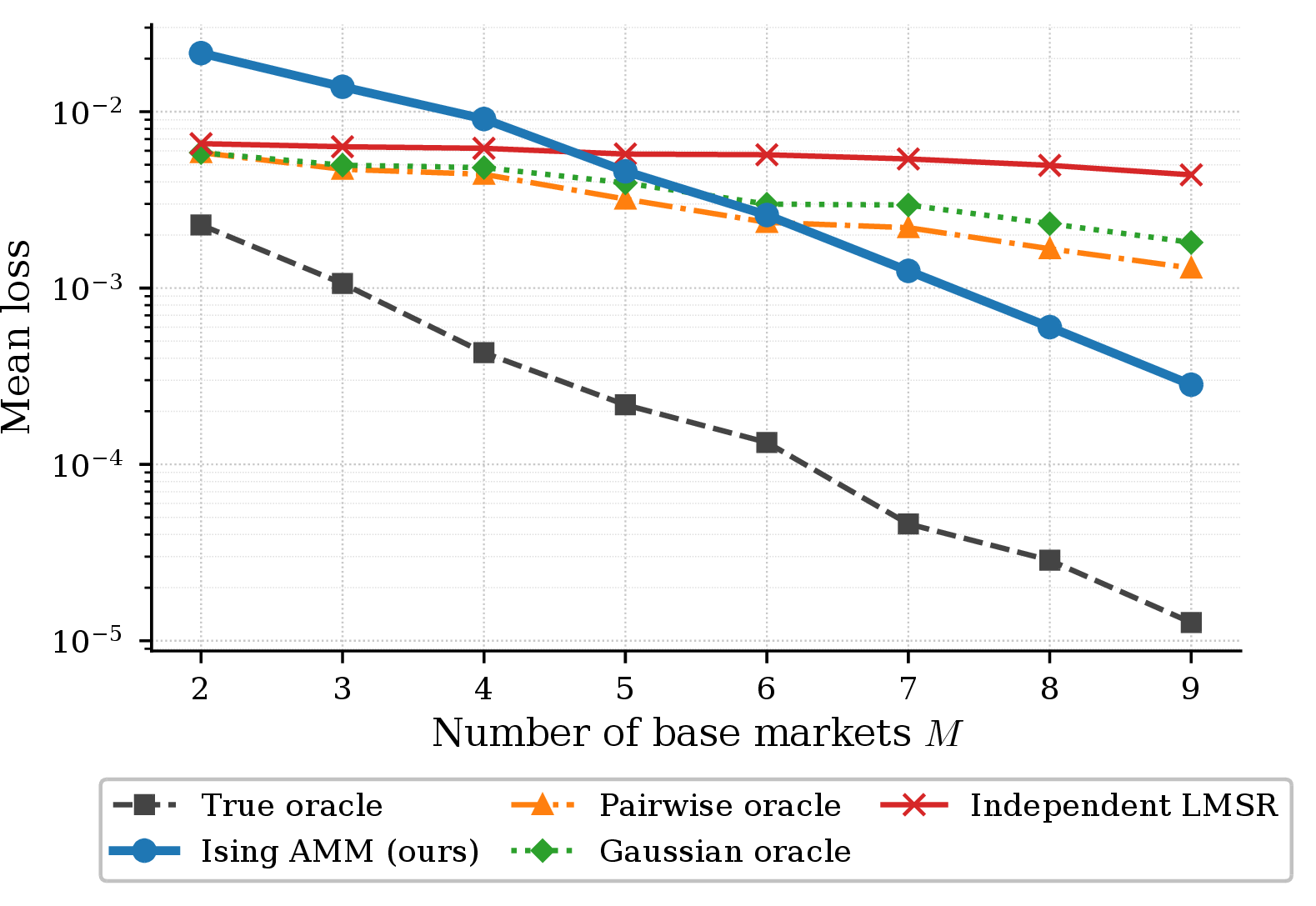

Figure 4: The ParlayMarket is the only non-oracle model whose loss decays exponentially with the number of base markets \(M\), in the presence of parlays; all other non-oracle models plateau or grow.. a — Mean LMSR loss per round per market \(\bar{\ell}_M\)., b — \(\mathrm{CVaR}_{95}\) loss per round per market.
| \(M\) | \(N_M\) | \(\ell_M\) | \(\ell_{M+1}/\ell_M\) | \(\ell_M \cdot 2^M\) | \(N_M \cdot \ell_M\) |
|---|---|---|---|---|---|
| 4 | 15 | \(\sim 0.0094\) | \(\sim 0.49\) | \(\sim 0.15\) | \(\sim 0.14\) |
| 5 | 31 | \(\sim 0.0048\) | \(\sim 0.50\) | \(\sim 0.15\) | \(\sim 0.15\) |
| 6 | 63 | \(\sim 0.0024\) | \(\sim 0.50\) | \(\sim 0.15\) | \(\sim 0.15\) |
| 7 | 127 | \(\sim 0.0012\) | \(\sim 0.50\) | \(\sim 0.15\) | \(\sim 0.15\) |
| 8 | 255 | \(\sim 0.0006\) | \(\sim 0.50\) | \(\sim 0.15\) | \(\sim 0.15\) |
| 9 | 511 | \(\sim 0.0003\) | — | \(\sim 0.15\) | \(\sim 0.15\) |
6.1.0.4 Price convergence.
Figure 5 shows the mean absolute error (MAE) between the AMM’s posted prices and the true probabilities over time, averaged across all \(N_M\) markets and all simulation runs, with \(\pm 1\sigma\) shading. The top panel shows the LMSR market-price MAE; the bottom panel shows the Ising marginal belief error for the Ising model. Both converge monotonically; the Ising belief error converges faster because belief propagation directly optimises the Ising objective, while the market-price error includes the additional LMSR rounding effect.

6.1.0.5 Parlay acceleration.
Consistent with Proposition 3, the advantage of the ParlayMarket is entirely contingent on the presence of parlay order flow. Figure 4 shows that with complete parlays the Ising AMM achieves the lowest non-oracle loss, decaying exponentially with \(M\). Figure 6 shows the complementary picture: when informed traders are restricted to base markets only, the model ranking completely reverses.
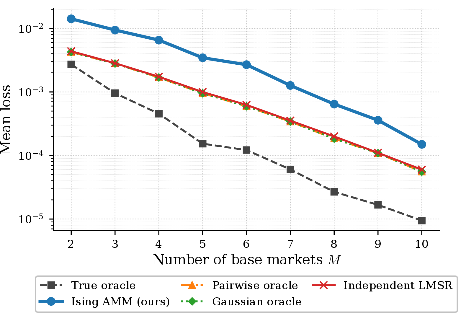
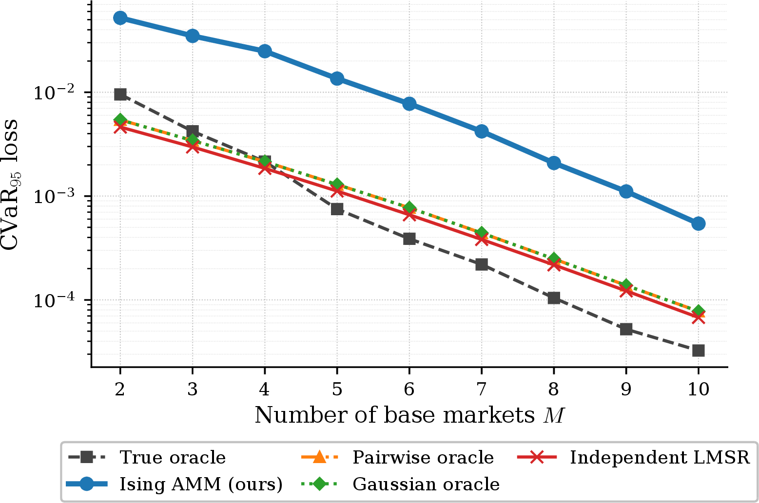
Figure 6: The ParlayMarket fails to perform better than even independent AMMs in the absence of parlay markets.. a — Mean LMSR loss per round per market \(\bar{\ell}_M\)., b — \(\mathrm{CVaR}_{95}\) loss per round per market.
6.2 Importance of Parlays for learning↩︎
6.2.0.1 Setup.
We run an ablation in which informed traders are restricted to the \(M\) base markets only - no parlay bets are placed - while all AMMs still maintain and price all \(N_M = 2^M - 1\) markets. Figures 4 and 6 show mean loss per round per market vs.\(M\) for both conditions.
6.2.0.2 The model ranking reverses completely.
With complete parlays (Figure 4), the ParlayMarket is the best-performing non-oracle model: it achieves the lowest per-round loss of all non-oracle AMMs, sitting just above the true oracle and well below every other model. The independent LMSR, pairwise oracle, and Gaussian oracle all incur substantially higher and exponentially growing losses as \(M\) increases, reaching \(\approx 2.24\), \(\approx 0.66\), and \(\approx 0.93\) per round respectively at \(M=9\).
Without parlays (Figure 6), the ranking completely reverses: the ParlayMarket now has the highest loss of all non-oracle models, while the independent LMSR, pairwise oracle, and Gaussian oracle cluster together at much lower values (\(\approx 0.02\)–\(0.06\) per round across all tested \(M\)). The y-axis scale tells the story: the no-parlay plot peaks at \(\approx 0.18\), while the with-parlay plot requires a scale of \(2.3\) - a \(13\times\) difference - just to accommodate the losses of the non-Ising models.
6.2.0.3 Why the ranking reverses.
The reversal reveals precisely what parlays provide: the gradient signal needed to calibrate the Ising joint belief model. Without parlays, the ParlayMarket receives gradient updates only from the \(M\) base markets. This is insufficient to pin down the \(\binom{M}{2}\) interaction parameters \(W_{ij}\) in any reasonable simulation length: the base-market signal is under-determined relative to the full Ising parameter space, so the model misprices joint events and incurs high loss. Simpler models - the pairwise oracle (which knows \(p_{ij}^*\) analytically) and the independent LMSR (which only needs to price \(M\) uncorrelated events) - do not face this calibration problem and therefore achieve low loss without parlays. With parlays, the situation reverses. Each parlay bet supplies a direct gradient signal on a specific joint event, giving the Ising model the rich information it needs to calibrate \((\boldsymbol{\theta}, \mathbf{W})\) from all \(N_M\) markets simultaneously (Proposition 3 and Figure 4). Once calibrated, belief propagation ensures that all \(N_M\) posted prices are globally consistent with the learned joint distribution, so adversaries cannot exploit mispriced correlations. The independent LMSR cannot use this information at all (it ignores correlations by design), and the pairwise and Gaussian oracles only capture lower-order structure - leaving them vulnerable to adversaries who trade higher-order parlays against their mispriced joint events.
6.2.0.4 Implication.
Parlays are not merely an efficiency accelerant: they are the primary information channel through which the ParlayMarket learns the joint distribution. Without them, the Ising model is the worst non-oracle performer; with them, it is the best. No other model tested achieves this reversal, confirming that the ParlayMarket and parlay markets are jointly necessary - neither is sufficient alone.
6.3 Robustness Under Noisy Informed Traders↩︎
6.3.0.1 Setup.
We repeat the complete-parlay simulation with the same parameters but vary the noise-trader fraction \(\alpha \in [0, 1]\): with probability \(\alpha\) the arriving trader submits a uniformly random price signal, and with probability \(1 - \alpha\) they are fully informed. Results at \(M = 9\) are extrapolated from direct simulations at \(M \in \{3, 4, 5\}\) using the clean \(M = 5 \to 9\) loss scaling.
6.3.0.2 Results.
Figure 7 (a) shows the per-market LMSR loss as a function of noise-trader fraction \(\alpha\) for \(M = 9\). The ParlayMarket’s loss grows gracefully with \(\alpha\)—it remains the best-performing non-oracle model across all noise levels tested—because the noisy gradient signal inflates the steady-state error while leaving the convergence rate largely unchanged. All models cross the break-even line only at high noise fractions, demonstrating robustness to realistic noise levels.
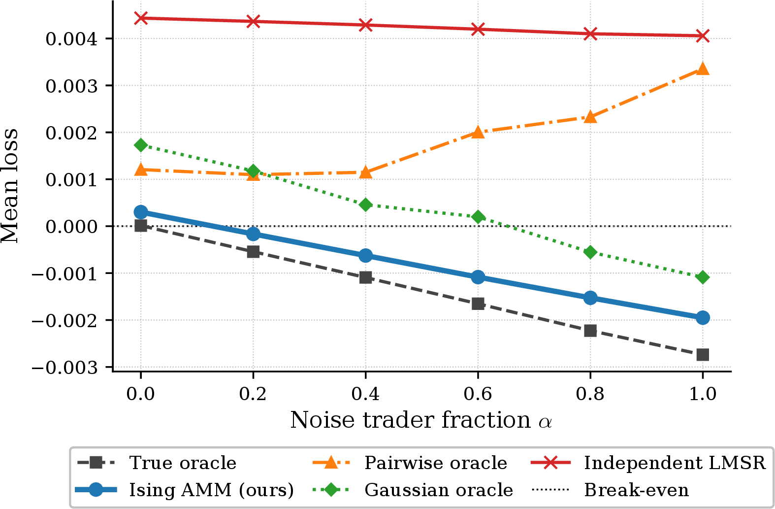
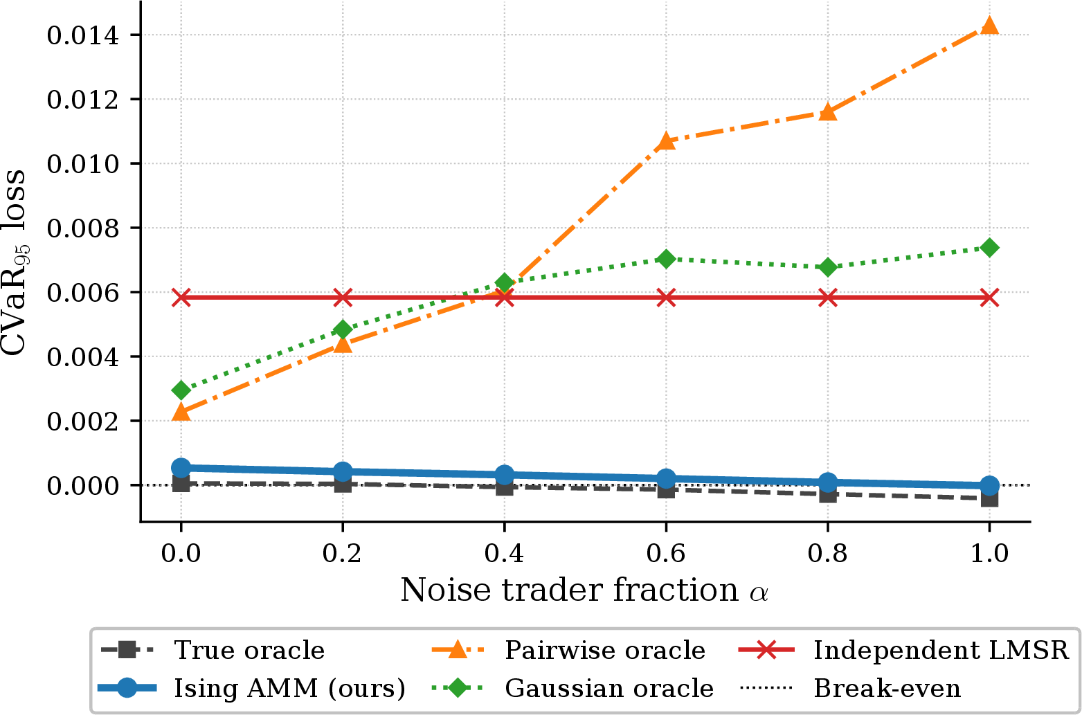
Figure 7: Per-market loss under varying noise-trader fractions (\(M = 9\), extrapolated from \(M \in \{3,4,5\}\) simulations). The ParlayMarket remains the best-performing non-oracle model across all noise levels; the break-even line is crossed only at high noise fractions.. a — Per-market loss vs.noise trader fraction \(\alpha\) (\(M = 9\))., b — \(\mathrm{CVaR}_{95}\) loss vs.noise trader fraction \(\alpha\) (\(M = 9\)).
6.4 Extension to Multinomial Markets↩︎
6.4.0.1 Setup.
All experiments above assume binary outcomes per base asset. We now evaluate whether the Ising AMM generalises to multinomial markets, where each base asset can resolve to one of \(K > 2\) outcomes. We run three configurations that vary the outcome structure and the nature of price jumps (e.g.smooth updates vs.discontinuous jumps between outcome clusters). In each case, we compare the Ising AMM against a True Oracle baseline (knows the true joint distribution exactly) and an Independent baseline (maintains a separate market maker per outcome, ignoring all correlations). The underlying trader model for these results is a straightforward generalization of the Gaussian scoring model, and the details are deferred to Appendix .
6.4.0.2 Results.
Figure 8 reports the key per-round statistics (mean, median, 95% VaR, and 95% CVaR of Loss / Step) across the three configurations. In every scenario the Ising AMM sits strictly between the True Oracle lower bound and the Independent baseline: it captures a large fraction of the correlation structure available to the oracle while outperforming the disjoint-market-maker strategy on all four statistics. The gap between Ising AMM and Independent is particularly pronounced in the tail-risk metrics (95% VaR and CVaR), indicating that joint modelling not only reduces average loss but also curtails the worst-case exposure that arises when correlated outcomes are priced independently. These results demonstrate that the Ising parameterisation and the parlay-driven gradient signal are not artefacts of the binary setting. The mechanism extends naturally to multinomial markets and retains its loss advantage over disjoint market makers even as the outcome space grows.


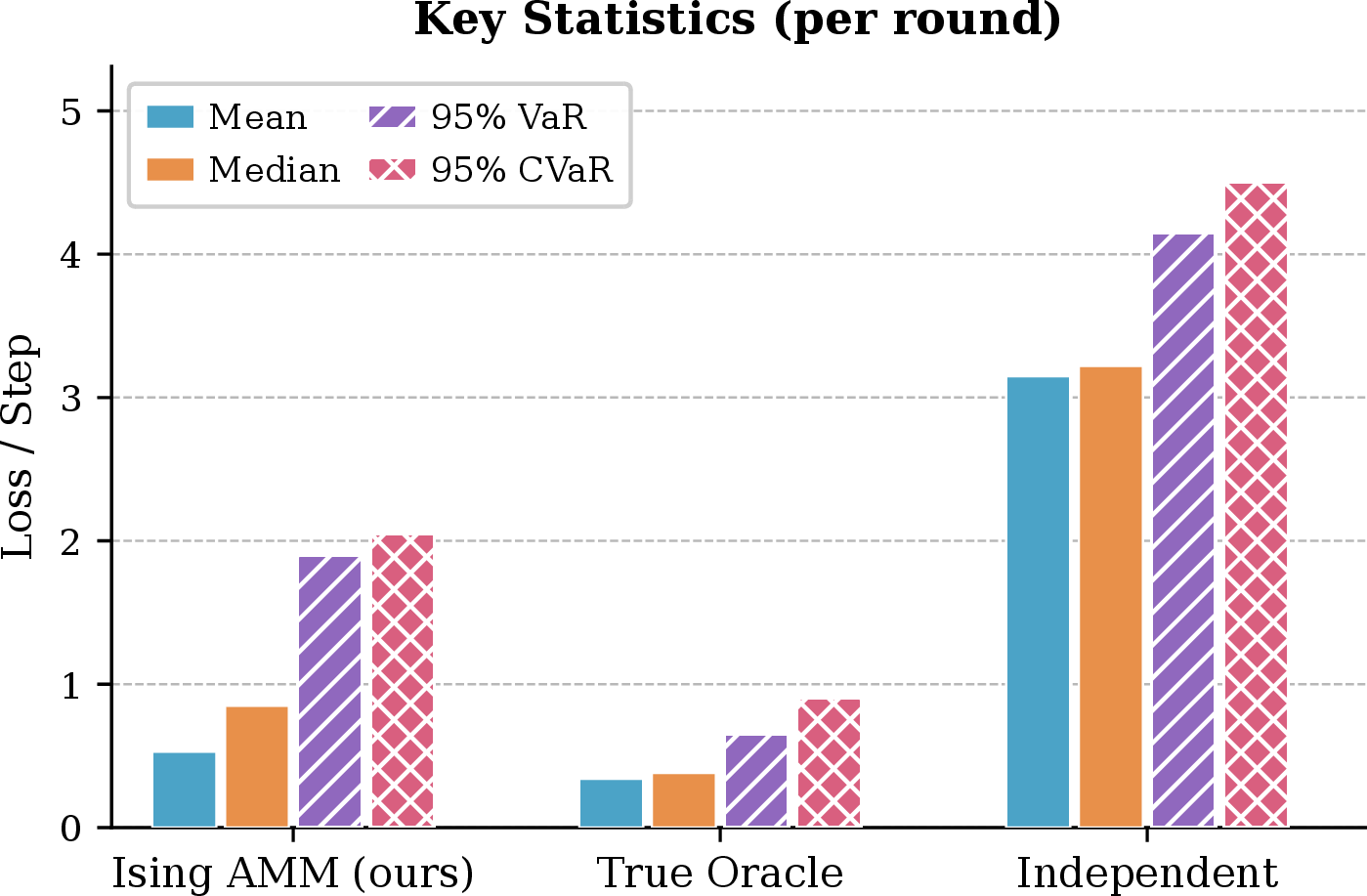
Figure 8: Key per-round statistics (Loss / Step) for three multinomial market configurations. In all cases the Ising AMM (ours) sits between the True Oracle lower bound and the Independent baseline, with the largest relative gain visible in the tail-risk measures (95% VaR and CVaR).. a — Five markets with \([2,3,4,4,5]\) outcomes, b — Eight markets with \([2,3,3,4,4,5,6,7]\) outcomes, c — Eight markets with \([2,3,3,4,4,5,6,7]\) outcomes, and random jumps
6.5 Empirical Market Performance↩︎
To evaluate whether these advantages survive outside the synthetic setting, we replay the mechanism on historical Kalshi data. The empirical study preserves three implementation details that are central to the practicality of the design.
6.5.0.1 Two execution settings.
We consider two execution settings. In a full-market emulation, base markets are modeled as LMSRs under the AMM, and the informative signal extracted from each trade is its target price: an informed trader is assumed to move the market to the price implied by her information. In a standalone market-maker emulation, base markets remain external and the AMM is used only as a shared quoting and underwriting engine for parlays; in that case the relevant signal is order flow - trade direction and share quantity - rather than the final market price. These two settings correspond to two distinct practical roles of the mechanism: a complete market design and a drop-in correlation-aware parlay market maker layered on top of an existing RFQ-style platform.
6.5.0.2 Real-market emulation.
The replay is performed on a real historical universe. We use Kalshi’s NBA slate for 2026-03-07, comprising 732 base markets across six games and 5,918 listed combo tickers with legs entirely inside this universe, spanning 2- through 10-leg parlays. To scale inference to clusters of this size, we train one Ising model per game cluster and use loopy belief propagation rather than exact enumeration. Each model is initialized from the first 30 candle mid-prices of its constituent legs, with fields initialized from median log-odds and couplings initialized at zero, after which the stream of candle updates and parlay trades is replayed chronologically. Candle updates train local fields, while parlay trades update both fields and interactions through the trade-implied target price.
6.5.0.3 Preprocessing.
The empirical setup explicitly addresses a key market imperfection: fee bias. Observed Kalshi combo execution prices are ask quotes rather than direct probability assessments, so they are systematically upward biased by platform markup. Training directly on these prices would therefore bias the learned joint model upward. To correct for this, we preprocess each observed trade into a canonical all-YES representation using the complement rule and inclusion–exclusion; for mixed YES/NO parlays, the additive fee cancels in the alternating expansion, yielding an approximately unbiased target in the model’s native parameterization. This correction is essential in practice: without it, parlay loss remains flatter and revenue is lower.
The full replay pipeline and all implementation details are described in Appendix 11. Table 4 shows that standalone ParlayMarket market maker achieves the strongest risk-adjusted liquidity-provider portfolio, with the highest Sharpe ratio among the non-native strategies while still accepting a large fraction of historical flow. The full AMM accepts all trades but exhibits lower ROI, likely because the observed RFQ flow contains substantial noise that a fully internalized LMSR-style implementation must absorb directly. Taken together, these results show that the empirical value of ParlayMarket pricing is strongest in the standalone market-maker regime: the model can be inserted into an existing platform, improve LP portfolio quality, and remain competitive on accepted quotes.
6.6 Summary↩︎
Across both synthetic and historical evaluations, the results support the same conclusion. A shared, learned representation of the joint distribution allows ParlayMarket to quote a combinatorially large family of contracts while controlling aggregate loss, using parlay order flow as a direct signal for dependence learning. In synthetic settings this produces the predicted scaling and convergence behavior; in historical replay it yields a practically useful correlation-aware quoting engine with strong risk-adjusted performance that can be readily deployed.
| Strategy | Accepted Trades | MM Win Rate | Net PnL | Sharpe | |
|---|---|---|---|---|---|
| Kalshi (execution price) | 5436 | 84.5% | $244,190.77 | 0.7151 | |
| Stand-alone MM (\(\theta_{\rm corr}\)) | 3973 | 86.8% | $113,984.58 | 1.0049 | |
| Full AMM | 5436 | 69.0% | $158,577.66 | 0.7062 |
7 Conclusion and limitations↩︎
In this paper, we showed that parlay trading can be incorporated into an automated market maker without requiring a separate pricing and risk-management process for every combination. The mechanism supports \(2^M\) base and joint contracts using only an \(O(M^2)\) shared representation, and correspondingly achieves \(O(M^2)\) aggregate information-retrieval loss rather than loss that scales with the full combinatorial market space. This shared structure also allows parlay order flow to serve as a direct signal for learning dependence structure. The empirical results further suggest that the mechanism is not only theoretically well-founded but close to deployable in practice: historical-market replay on Kalshi data shows that, in the standalone market-maker setting, correlation-aware quoting remains competitive under observed prices, RFQ flow, and realistic execution constraints.
An important scope condition of the current framework is that the traded contracts are assumed to already be expressed in a structurally coherent binary form. In many practical settings, this representation must itself be constructed before correlation-aware pricing becomes meaningful. For example, families of mutually exclusive outcomes may satisfy constraints such as \(\sum_{i=1}^k X_i = 1\), even though the underlying latent process remains stochastic. In such cases, a separate preprocessing or structural-learning layer is needed to map raw market data into variables on which the assumptions of the AMM hold. We illustrate one such preprocessing step in the evaluation section. This suggests a broader architecture for automated parlay markets: a structural layer that identifies and normalizes the relevant event representation, followed by a pricing layer such as ParlayMarket that provides automated execution and, as a secondary benefit, elicits dependence from the resulting trade flow.
8 RFQ Details↩︎
8.1 Combo Mispricing for Independent Events↩︎
Our experiments show that the RFQ combo market fails Property 3 in a basic sense: combo prices do not reliably encode joint probabilities even in independent cases. We consider two-leg combos whose legs are drawn from different leagues (NBA and ATP tennis) so that the events are naturally close to independent. We fetch the base market prices for legs and compare them to the best quote we receive from the combo market for the 2-leg combo. Detailed quotes and prices for this experiment are shown in Table 5.
Under probabilistic pricing, the combo YES price should be approximately the product of the two leg YES prices. All 33 quoted prices exceed the independence benchmark. Moreover, and more decisively, 13 of the 33 quotes (39%) violate the Fréchet upper bound \(P(A \cap B) \leq \min(P(A), P(B))\)—a constraint that holds under any joint probability distribution, regardless of correlation structure (Table 6).
| Leg 1 | Leg 2 | \(p_1 \cdot p_2\) | Quoted | \(\Delta\) |
|---|---|---|---|---|
| 72c | 88c | 63.4c | 72c | 8.6c |
| 72c | 37c | 26.6c | 70c | 43.4c |
| 72c | 15c | 10.8c | 31c | 20.2c |
| 72c | 14c | 10.1c | 30c | 19.9c |
| 72c | 41c | 29.5c | 50c | 20.5c |
| 72c | 20c | 14.4c | 34c | 19.6c |
| 72c | 82c | 59.0c | 63c | 4.0c |
| 72c | 79c | 56.9c | 62c | 5.1c |
| 72c | 17c | 12.2c | 14c | 1.8c |
| 72c | 42c | 30.2c | 31c | 0.8c |
| 72c | 30c | 21.6c | 25c | 3.4c |
| 29c | 88c | 25.5c | 29c | 3.5c |
| 29c | 37c | 10.7c | 29c | 18.3c |
| 29c | 15c | 4.4c | 29c | 24.7c |
| 29c | 14c | 4.1c | 24c | 19.9c |
| 29c | 41c | 11.9c | 29c | 17.1c |
| 29c | 20c | 5.8c | 26c | 20.2c |
| 29c | 82c | 23.8c | 27c | 3.2c |
| 29c | 79c | 22.9c | 26c | 3.1c |
| 29c | 17c | 4.9c | 6c | 1.1c |
| 29c | 42c | 12.2c | 13c | 0.8c |
| 29c | 30c | 8.7c | 29c | 20.3c |
| 82c | 88c | 72.2c | 82c | 9.8c |
| 82c | 37c | 30.3c | 79c | 48.7c |
| 82c | 15c | 12.3c | 80c | 67.7c |
| 82c | 14c | 11.5c | 80c | 68.5c |
| 82c | 41c | 33.6c | 35c | 1.4c |
| 82c | 20c | 16.4c | 80c | 63.6c |
| 82c | 82c | 67.2c | 72c | 4.8c |
| 82c | 79c | 64.8c | 70c | 5.2c |
| 82c | 17c | 13.1c | 14c | 0.9c |
| 82c | 42c | 34.4c | 35c | 0.6c |
| 82c | 30c | 24.6c | 45c | 20.4c |
| Leg 1 | Leg 2 | \(p_1 \cdot p_2\) | \(\min(p_1,p_2)\) | Quoted | \(Q / \min\) |
|---|---|---|---|---|---|
| 82c | 14c | 11.5c | 14c | 80c | \(5.71\times\) |
| 82c | 15c | 12.3c | 15c | 80c | \(5.33\times\) |
| 82c | 20c | 16.4c | 20c | 80c | \(4.00\times\) |
| 82c | 37c | 30.3c | 37c | 79c | \(2.14\times\) |
| 72c | 14c | 10.1c | 14c | 30c | \(2.14\times\) |
| 72c | 15c | 10.8c | 15c | 31c | \(2.07\times\) |
| 29c | 15c | 4.4c | 15c | 29c | \(1.93\times\) |
| 72c | 37c | 26.6c | 37c | 70c | \(1.89\times\) |
| 82c | 30c | 24.6c | 30c | 45c | \(1.50\times\) |
| 72c | 20c | 14.4c | 20c | 34c | \(1.70\times\) |
| 29c | 14c | 4.1c | 14c | 24c | \(1.71\times\) |
| 72c | 41c | 29.5c | 41c | 50c | \(1.22\times\) |
| 29c | 20c | 5.8c | 20c | 26c | \(1.30\times\) |
8.2 Quote Aggregation to Tighten Spread↩︎
We test whether multiple market makers materially tighten combo quotes. Let \(S1\) denote the best single-maker spread and \(S2\) the mixed spread obtained by taking the best YES quote and best NO quote across all market makers. From Table 7 the average \(S1\) is 12.08c and the average \(S2\) is 11.89c, so quote aggregation improves execution by only 0.19c on average. This pattern also holds across leg counts shown on Table 8: for 2-leg combos, average spreads remain very wide (26.02c for \(S1\), 24.30c for \(S2\)); for 3+ leg combos, the improvement is negligible. Overall, the presence of multiple market makers does not generate meaningful competitive tightening in combo markets.
| Metric | Value |
|---|---|
| Average quotes per combo | 4.5 |
| Best single quote spread (\(S1\)) | 12.08c |
| Best mixed quote spread (\(S2\)) | 11.89c |
| Mixed-quote improvement (\(S1 - S2\)) | 0.19c |
| Leg count | Count | Avg.\(S1\) (cents) | Avg.\(S2\) (cents) |
|---|---|---|---|
| 2 | 43 | 26.02 | 24.30 |
| 3 | 58 | 22.19 | 22.19 |
| 4 | 56 | 14.80 | 14.73 |
| 5+ | 392 | 8.66 | 8.60 |
9 Mathematical Proofs↩︎
This appendix supplies proofs and supporting derivations for the claims stated in Section 5. In particular, it supports the Property 1 bound in Subsection 5.1, Theorem 1, Proposition 1, Lemma 1, Proposition 2, and Proposition 3. Throughout this appendix we write \(\phi\) for the parameter vector \(\boldsymbol{\varphi}\) from Section 5.
9.1 Proof supporting Property 1 in Subsection 5.1↩︎
Proof of the liquidity-consistency bound in the Property 1 paragraph of Subsection 5.1. Fix any market \(S\) and let \(z_S\) denote the YES-minus-NO share imbalance in the corresponding two-outcome LMSR book. With common liquidity parameter \(b\), the LMSR YES price is \[p_S(z_S) = \frac{e^{z_S/b}}{1+e^{z_S/b}}.\] After a small YES order of size \(x\), the new imbalance is \(z_S+x\), so the local price impact is \[I_S(x;\phi) := p_S(z_S+x)-p_S(z_S).\] Since \[p_S'(z_S) = \frac{1}{b}\,p_S(z_S)\bigl(1-p_S(z_S)\bigr),\] Taylor expansion gives \[I_S(x;\phi) = \frac{x}{b}\,p_S^{\phi}\bigl(1-p_S^{\phi}\bigr)+O(x^2),\] which is the local-impact formula displayed in Subsection 5.1.
Assume now that all active quotes lie in the operating region \[p_S^{\phi}\in[\varepsilon,1-\varepsilon] \qquad \text{for every active }S.\] Then \[\varepsilon(1-\varepsilon) \le p_S^{\phi}\bigl(1-p_S^{\phi}\bigr) \le \frac{1}{4}.\] Hence the directional derivative of price impact at the origin satisfies \[\frac{\partial_x I_S(0;\phi)}{\partial_x I_{S'}(0;\phi)} = \frac{p_S^{\phi}(1-p_S^{\phi})}{p_{S'}^{\phi}(1-p_{S'}^{\phi})} \in \bigl[4\varepsilon(1-\varepsilon),\,1/(4\varepsilon(1-\varepsilon))\bigr].\] By continuity, the same comparability holds for all sufficiently small admissible trades \(x\). Thus small orders induce comparable local price impact across base and parlay contracts. Because all quoted probabilities are functions of the same shared state \(\phi\), every real trade also shifts all related prices immediately, which is exactly the liquidity-consistency claim made in the Property 1 paragraph of Subsection 5.1. ◻
9.2 Proofs for Subsection 5.3↩︎
9.2.0.1 Common notation.
Let \[\mathcal{E}_2 := \bigl\{\{i\}:1\le i\le M\bigr\} \cup \bigl\{\{i,j\}:1\le i<j\le M\bigr\}.\] For a traded event \(E\subseteq [M]\), write \[q_E(\phi) := P_\phi\!\Big(\bigcap_{i\in E}\{X_i=1\}\Big), \qquad p_E^\ast := P^\ast\!\Big(\bigcap_{i\in E}\{X_i=1\}\Big),\] and \[\ell_E(\phi):=\mathrm{CE}(p_E^\ast,q_E(\phi)) = -p_E^\ast \log q_E(\phi) - (1-p_E^\ast)\log(1-q_E(\phi)).\] If the market corresponding to \(E\) is sampled with probability \(\lambda_E>0\), define \[L(\phi):=\sum_{E\in\mathcal{E}_2}\lambda_E\,\ell_E(\phi).\] This is the same singleton-and-pairwise composite objective as \(\mathcal{L}\) in 4 , written with a shorter symbol in the appendix. Let \[T(X):=\bigl(X_1,\dots,X_M,\,(X_iX_j)_{1\le i<j\le M}\bigr)\] denote the vector of sufficient statistics. We assume throughout that the target moment vector \[m^\ast := \bigl(p_i^\ast,\; p_{ij}^\ast\bigr)_{1\le i<j\le M}\] lies in the interior of the pairwise marginal polytope, so that it is realizable by a unique pairwise Ising parameter \(\phi^\star\).
9.2.0.2 Expected gradient of the sampled update.
The sampled update in 5 is exactly the stochastic-gradient step for the composite loss 4 . Indeed, for any traded event \(E\), \[\nabla_\phi \ell_E(\phi) = \frac{q_E(\phi)-p_E^\ast}{q_E(\phi)(1-q_E(\phi))}\,\nabla_\phi q_E(\phi).\] By the covariance identity used in Subsection 5.3, \[\nabla_\phi q_E(\phi) = \operatorname{Cov}_\phi\!\bigl(T(X),\mathbf{1}_E\bigr) = q_E(\phi)\Bigl(\mathbb{E}_\phi[T(X)\mid E]-\mathbb{E}_\phi[T(X)]\Bigr).\] Hence \[\nabla_\phi \ell_E(\phi) = \frac{q_E(\phi)-p_E^\ast}{1-q_E(\phi)} \Bigl(\mathbb{E}_\phi[T(X)\mid E]-\mathbb{E}_\phi[T(X)]\Bigr),\] which is exactly the vector form of the marketwise update described after 5 . Therefore, if \(E_t\) denotes the event traded at round \(t\), then \[\phi_{t+1}=\phi_t-\eta g_t, \qquad \mathbb{E}[g_t\mid \phi_t]=\nabla L(\phi_t).\]
Proof of the moment-matched target claim in Subsection 5.3. Because the mean dynamics are gradient descent on \(L\), it suffices to identify the unique minimizer of \(L\). Let \(\phi^\star\) be the unique Ising parameter whose singleton and pairwise moments equal \((p_i^\ast,p_{ij}^\ast)\). Such a parameter exists and is unique because the pairwise Ising family is a finite exponential family with strictly convex log-partition function, so the map from natural parameters to interior moments is one-to-one.
For every \(E\in\mathcal{E}_2\), \[\ell_E(\phi)-\ell_E(\phi^\star) = \mathrm{CE}(p_E^\ast,q_E(\phi))-\mathrm{CE}(p_E^\ast,p_E^\ast) = \mathrm{KL}\!\bigl(\mathrm{Bern}(p_E^\ast)\,\|\,\mathrm{Bern}(q_E(\phi))\bigr) \ge 0.\] Summing with weights \(\lambda_E\) gives \[L(\phi)-L(\phi^\star) = \sum_{E\in\mathcal{E}_2}\lambda_E\, \mathrm{KL}\!\bigl(\mathrm{Bern}(p_E^\ast)\,\|\,\mathrm{Bern}(q_E(\phi))\bigr) \ge 0.\] Equality holds if and only if \(q_E(\phi)=p_E^\ast\) for every traded event \(E\), that is, if and only if \(\phi\) matches all singleton and pairwise moments. By injectivity of the Ising moment map on the interior of the marginal polytope, this happens only at \(\phi=\phi^\star\).
Thus \(\phi^\star\) is the unique global minimizer of \(L\). Since the mean update is \(-\eta \nabla L(\phi)\), \(\phi^\star\) is also the unique fixed point of the mean dynamics. Finally, the maximum-entropy characterization in the moment-matched target paragraph follows from the standard Lagrange-duality argument for finite exponential families: among all distributions on \(\{0,1\}^M\) with the prescribed first and second moments, the entropy maximizer has density proportional to \(\exp(\langle \phi^\star,T(x)\rangle)\), which is exactly the pairwise Ising law. ◻
Proof of Proposition 1 (local strong-convexity form used in the convergence argument). Let \[m(\phi):=\bigl(q_E(\phi)\bigr)_{E\in\mathcal{E}_2}\in\mathbb{R}^d, \qquad J(\phi):=\nabla_\phi m(\phi)\in\mathbb{R}^{d\times d}.\] Write \(L=F\circ m\), where \[F(u):=\sum_{E\in\mathcal{E}_2}\lambda_E\,\mathrm{CE}(p_E^\ast,u_E).\] Since \[\frac{\partial}{\partial u_E}\mathrm{CE}(p_E^\ast,u_E) = \frac{u_E-p_E^\ast}{u_E(1-u_E)}, \qquad \frac{\partial^2}{\partial u_E^2}\mathrm{CE}(p_E^\ast,u_E) = \frac{1}{u_E(1-u_E)},\] the chain rule gives \[\nabla^2 L(\phi) = J(\phi)^\top D(\phi)J(\phi) + \sum_{E\in\mathcal{E}_2}\lambda_E \frac{q_E(\phi)-p_E^\ast}{q_E(\phi)(1-q_E(\phi))} \,\nabla_\phi^2 q_E(\phi),\] where \[D(\phi) = \operatorname{diag}\!\Bigl(\frac{\lambda_E}{q_E(\phi)(1-q_E(\phi))}\Bigr)_{E\in\mathcal{E}_2}.\] At \(\phi=\phi^\star\) we have \(q_E(\phi^\star)=p_E^\ast\) for every \(E\), so the second term vanishes and therefore \[\nabla^2 L(\phi^\star) = J(\phi^\star)^\top D^\star J(\phi^\star), \qquad D^\star = \operatorname{diag}\!\Bigl(\frac{\lambda_E}{p_E^\ast(1-p_E^\ast)}\Bigr)_{E\in\mathcal{E}_2}.\] Assume now that \(J(\phi^\star)\) has full rank and that \(p_E^\ast\in[\varepsilon,1-\varepsilon]\) for every traded event \(E\). Then \(D^\star\succ 0\), hence \(\nabla^2 L(\phi^\star)\succ 0\). Let \[\mu_0:=\lambda_{\min}\!\bigl(\nabla^2 L(\phi^\star)\bigr)>0.\] Because \(\nabla^2L\) is continuous, there exists a neighborhood \(U\) of \(\phi^\star\) such that \[\nabla^2L(\phi)\succeq \frac{\mu_0}{2}I \qquad \text{for all }\phi\in U.\] By the Hessian characterization of strong convexity, \(L\) is \(\mu\)-strongly convex on \(U\) with \(\mu=\mu_0/2\).
This is the local strong-convexity statement needed in the proof of Theorem 1. The explicit Hessian values quoted in Proposition 1 at the uninformative initialization \(\phi=0\) are obtained by evaluating the same Fisher blocks under the uniform product measure. ◻
Proof of Theorem 1. Let \(U\) be the neighborhood from the previous proof, and assume that all iterates remain in \(U\). Write \[e_t:=\phi_t-\phi^\star.\] Because the sampled gradient is unbiased, we may write \[g_t=\nabla L(\phi_t)+\zeta_t, \qquad \mathbb{E}[\zeta_t\mid \phi_t]=0, \qquad \mathbb{E}[\|\zeta_t\|^2\mid \phi_t]\le \sigma^2.\] Let \(L_g\) denote a gradient-Lipschitz constant of \(L\) on \(U\). Then \[e_{t+1}=e_t-\eta \nabla L(\phi_t)-\eta \zeta_t.\] Taking conditional expectations and using \(\mathbb{E}[\zeta_t\mid \phi_t]=0\), \[\mathbb{E}\!\left[\|e_{t+1}\|^2\mid \phi_t\right] = \|e_t\|^2 -2\eta\langle \nabla L(\phi_t),e_t\rangle +\eta^2\|\nabla L(\phi_t)\|^2 +\eta^2\mathbb{E}\!\left[\|\zeta_t\|^2\mid \phi_t\right].\] Local strong convexity gives \[\langle \nabla L(\phi_t),e_t\rangle \ge \mu \|e_t\|^2,\] and \(L_g\)-smoothness gives \[\|\nabla L(\phi_t)\| = \|\nabla L(\phi_t)-\nabla L(\phi^\star)\| \le L_g \|e_t\|.\] Hence \[\mathbb{E}\!\left[\|e_{t+1}\|^2\mid \phi_t\right] \le \bigl(1-2\eta\mu+\eta^2 L_g^2\bigr)\|e_t\|^2+\eta^2\sigma^2.\] Set \[\rho:=1-2\eta\mu+\eta^2L_g^2.\] Taking full expectations and iterating the recursion yields \[\mathbb{E}\|e_t\|^2 \le \rho^t \|e_0\|^2 + \eta^2\sigma^2\sum_{s=0}^{t-1}\rho^s \le \rho^t \|e_0\|^2 + \frac{\eta^2\sigma^2}{1-\rho} = \rho^t \|e_0\|^2 + \frac{\eta\sigma^2}{2\mu-\eta L_g^2}.\] This is the precise finite-\(\eta\) estimate underlying the display in Theorem 1.
If \(\eta\le \mu/L_g^2\), then \(\rho\le 1-\eta\mu\), so \[\mathbb{E}\|e_t\|^2 \le (1-\eta\mu)^t\|e_0\|^2+\frac{2\eta\sigma^2}{\mu}.\] In the small-step regime, \[\rho=1-2\eta\mu+O(\eta^2), \qquad \frac{\eta\sigma^2}{2\mu-\eta L_g^2} = \frac{\eta\sigma^2}{2\mu}+O(\eta^2),\] which is exactly the simplified form quoted in Subsection 5.3. ◻
Proof of the \(O(\log T)\) cumulative-regret statement following 6 . Let \(L_t(\phi):=\ell_{E_t}(\phi)\) be the random round-\(t\) loss, where \(E_t\) is the market sampled at round \(t\). Because \(E_t\) is sampled with probabilities \((\lambda_E)_{E\in\mathcal{E}_2}\), \[\mathbb{E}[L_t(\phi_t)-L_t(\phi^\star)\mid \phi_t] = L(\phi_t)-L(\phi^\star).\] Now take the decaying step size \(\eta_t=c/t\). From the same recursion as in the proof of Theorem 1, \[\mathbb{E}\|\phi_t-\phi^\star\|^2\le \frac{C}{t}\] for some constant \(C>0\). Since \(L\) is \(L_g\)-smooth and \(\nabla L(\phi^\star)=0\), \[L(\phi_t)-L(\phi^\star) \le \frac{L_g}{2}\|\phi_t-\phi^\star\|^2.\] Therefore \[\mathbb{E}\!\left[\sum_{t=1}^T \bigl(L_t(\phi_t)-L_t(\phi^\star)\bigr)\right] = \sum_{t=1}^T \mathbb{E}\bigl[L(\phi_t)-L(\phi^\star)\bigr] \le \frac{L_g C}{2}\sum_{t=1}^T \frac{1}{t} \le \frac{L_g C}{2}(1+\log T).\] Thus the expected cumulative excess loss is \(O(\log T)\), exactly as stated after 6 . ◻
9.3 Proofs for Subsection 5.4↩︎
Proof of Lemma 1. Fix a market \(S\) and define \[f(p):=\mathrm{KL}(p_S^\ast\|p) = p_S^\ast\log\frac{p_S^\ast}{p} +(1-p_S^\ast)\log\frac{1-p_S^\ast}{1-p}.\] Then \(f(p_S^\ast)=0\) and \(f'(p_S^\ast)=0\), while \[f''(p) = \frac{p_S^\ast}{p^2}+\frac{1-p_S^\ast}{(1-p)^2}.\] In particular, \[f''(p_S^\ast)=\frac{1}{p_S^\ast(1-p_S^\ast)}.\] By Taylor’s theorem, for \(p\) in a sufficiently small neighborhood of \(p_S^\ast\), \[\mathrm{KL}(p_S^\ast\|p) = \frac{(p-p_S^\ast)^2}{2p_S^\ast(1-p_S^\ast)} + O\!\bigl(|p-p_S^\ast|^3\bigr).\] Next apply the mean-value theorem to the map \(\phi\mapsto p_S^\phi\). For \(\phi\) in a small neighborhood \(U\) of \(\phi^\star\), \[|p_S^\phi-p_S^\ast| \le \sup_{\tilde{\phi}\in U}\|\nabla p_S^{\tilde{\phi}}\|\,\|\phi-\phi^\star\|.\] Substituting this into the quadratic expansion above gives \[b\,\mathrm{KL}(p_S^\ast\|p_S^\phi) \le \frac{b}{2} \left( \sup_{\tilde{\phi}\in U} \frac{\|\nabla p_S^{\tilde{\phi}}\|^2}{p_S^\ast(1-p_S^\ast)} \right) \|\phi-\phi^\star\|^2 + O\!\bigl(\|\phi-\phi^\star\|^3\bigr).\] After shrinking \(U\) if necessary, the cubic remainder is dominated by the quadratic term, so the local bound in Lemma 1 follows with \[\Lambda_S := \sup_{\tilde{\phi}\in U} \frac{\|\nabla p_S^{\tilde{\phi}}\|^2}{p_S^\ast(1-p_S^\ast)}.\] The value \(\Lambda_S=1/4\) quoted in Subsection 5.4 is the corresponding baseline constant obtained by evaluating the same gradient expression at the symmetric initialization \(\phi=0\). ◻
Proof of Proposition 2 and of the mean-loss corollary stated afterward. For the complete-parlay regime, let \[N_M:=2^M-1.\] Let \(\ell_t\) denote the expected LMSR monetary loss incurred at round \(t\) by the market that is actually traded. Define the family-average quadratic sensitivity \[\bar\Lambda_M := \frac{1}{N_M} \sum_{\varnothing\neq S\subseteq[M]} \sup_{\phi\in U} \frac{\|\nabla p_S^\phi\|^2}{p_S^\ast(1-p_S^\ast)}.\] Assume the following three properties hold with constants independent of \(M\): \[\begin{align} \text{(A1)}\qquad \mathbb{E}\|\phi_t-\phi^\star\|^2 &\le C_0 \|\phi^\star\|^2 e^{-c\eta t}+C_1\eta, \\ \text{(A2)}\qquad \bar\Lambda_M &\le C_2, \\ \text{(A3)}\qquad \|\phi^\star\|^2 &=O(M^2\rho^2). \end{align}\] Condition (A1) is the transient-plus-noise-floor estimate inherited from Theorem 1; (A2) is the uniform average sensitivity bound needed to convert parameter error into monetary loss through Lemma 1; and (A3) is the weak-correlation scaling of the target interaction vector used in the text.
For the market \(S_t\) traded at round \(t\), Lemma 1 gives \[\mathbb{E}[\ell_t\mid S_t=S] \le \frac{b}{2} \left( \sup_{\phi\in U} \frac{\|\nabla p_S^\phi\|^2}{p_S^\ast(1-p_S^\ast)} \right) \mathbb{E}\|\phi_t-\phi^\star\|^2.\] Averaging over the uniformly sampled market family therefore yields \[\mathbb{E}[\ell_t] \le \frac{b\bar\Lambda_M}{2}\, \mathbb{E}\|\phi_t-\phi^\star\|^2 \le \frac{b C_2}{2}\Bigl(C_0\|\phi^\star\|^2 e^{-c\eta t}+C_1\eta\Bigr).\]
Summing the transient term over all \(t\ge 0\) and using \(\sum_{t\ge 0}e^{-c\eta t}=O(1/\eta)\), we obtain \[L_{\mathrm{transient}} \le \sum_{t\ge 0}\frac{bC_0C_2}{2}\|\phi^\star\|^2 e^{-c\eta t} = O\!\left(\frac{b\|\phi^\star\|^2}{\eta}\right) = O\!\left(\frac{b\rho^2 M^2}{\eta}\right),\] which is the transient bound stated in Proposition 2.
The steady-state per-round loss is obtained from the \(C_1\eta\) term: \[L_{\mathrm{ss,round}} = O(b\eta).\] This is the second display in Proposition 2.
Finally, the mean loss per listed market discussed at the end of Subsection 5.4 satisfies \[\bar\ell_M = \frac{1}{N_M T} \sum_{t=1}^T \mathbb{E}[\ell_t] \le \frac{L_{\mathrm{transient}}}{N_M T} + \frac{L_{\mathrm{ss,round}}}{N_M}.\] Hence \[\bar\ell_M = O\!\left(\frac{b\rho^2M^2}{\eta N_M T}\right) + O\!\left(\frac{b\eta}{N_M}\right).\] For \(T\to\infty\), the steady-state term dominates, so \[\bar\ell_M = O\!\left(\frac{b\eta}{N_M}\right) = O(b\eta\,2^{-M}).\] Since \(N_M=2^M-1\), \[\frac{\bar\ell_{M+1}}{\bar\ell_M} \longrightarrow \frac{N_M}{N_{M+1}} = \frac{2^M-1}{2^{M+1}-1} \longrightarrow \frac{1}{2}.\] This proves the halving-law corollary stated after Proposition 2. ◻
9.3.0.1 Remark on shadow trades.
The previous proof shows exactly where shadow trades enter the argument in Subsection 5.4: they are part of the mechanism that makes a uniform-in-\(M\) bound such as (A1) plausible. Without shadow repricing, parameters are updated only from direct order flow in their own markets, so the steady-state term in (A1) need not remain \(O(\eta)\) uniformly in \(M\); once that uniform bound fails, the aggregate loss guarantee in Proposition 2 can fail as well.
9.4 Proofs for Subsection 5.5↩︎
Proof of Proposition 3. Let \[\mathcal{E}_+ := \mathcal{E}_2 \cup \{S\subseteq [M]: |S|\ge 3,\;\lambda_S>0\},\] and define the augmented composite loss \[L^+(\phi):=\sum_{E\in \mathcal{E}_+}\lambda_E\,\mathrm{CE}(p_E^\ast,q_E(\phi)).\] This is the appendix shorthand for the augmented objective \(\mathcal{L}^+\) used in Proposition 3. Assume there exists a parameter \(\phi^\dagger\) such that \[q_E(\phi^\dagger)=p_E^\ast \qquad \text{for every }E\in \mathcal{E}_+,\] and that the augmented Jacobian \(J_+(\phi^\dagger)\) has full rank.
Exactly as in the proof of Proposition 1, the Hessian at \(\phi^\dagger\) is \[\nabla^2L^+(\phi^\dagger) = \sum_{E\in \mathcal{E}_+} \frac{\lambda_E}{p_E^\ast(1-p_E^\ast)} \,\nabla q_E(\phi^\dagger)\nabla q_E(\phi^\dagger)^\top.\] Split the sum into baseline events and higher-order events: \[\nabla^2L^+(\phi^\dagger) = \nabla^2L(\phi^\dagger) + \sum_{\substack{S\subseteq [M]\\ |S|\ge 3}} \frac{\lambda_S}{p_S^\ast(1-p_S^\ast)} \,\nabla q_S(\phi^\dagger)\nabla q_S(\phi^\dagger)^\top.\] Every added term is positive semidefinite, so \[\nabla^2L^+(\phi^\dagger)-\nabla^2L(\phi^\dagger)\succeq 0.\] Hence the local strong-convexity constant cannot decrease: \[\mu_{\mathrm{eff}}\ge \mu.\] Moreover, if one of the added rank-one terms has nonzero projection on a weakest-curvature eigendirection of \(\nabla^2L(\phi^\dagger)\), then \(\mu_{\mathrm{eff}}>\mu\), which is exactly the curvature improvement summarized in 6 and in item 1 of Proposition 3.
Applying Theorem 1 with \(L^+\) in place of \(L\) yields the improved contraction factor and the smaller steady-state error floor in item 2. Averaging the resulting bound over \(t\le T\) gives \[\bar\varepsilon_T^2 := \frac{1}{T}\sum_{t=1}^T \mathbb{E}\|\phi_t-\phi^\dagger\|^2 \le C\left( \frac{\|\phi_0-\phi^\dagger\|^2}{\eta \mu_{\mathrm{eff}} T} +\eta \right)\] for a constant \(C\) depending only on local smoothness and variance parameters. Therefore any quadratic price–loss bound of the form \[\ell_{\mathrm{mon}}(t)\le C_b \|\phi_t-\phi^\dagger\|^2\] immediately implies the improved average-loss conclusion in item 3. ◻
10 Multinomial Gaussian Scoring Model↩︎
This appendix describes the generalization of the binary Gaussian scoring model (Section 3.2) to categorical markets used in Section 6.4.
10.0.0.1 Categorical markets.
We consider \(M\) base markets where market \(i\) can resolve to one of \(K_i \geq 2\) mutually exclusive outcomes. The experiment in Section 6.4 uses two configurations: \(\mathbf{K} = [2,3,4,4,5]\) and \(\mathbf{K} = [2,3,3,4,4,5,6,7]\), giving total outcome spaces of \(\prod_i K_i = 480\) and \(241{,}920\) respectively.
10.0.0.2 Score process and threshold model.
Each market \(i\) is driven by an underlying score \(S_i(t) \in \mathbb{R}\) following correlated arithmetic Brownian motion \[dS_i(t) = \sigma\, dW_i(t), \qquad \mathrm{Cov}(dW_i, dW_j) = \rho_{ij}\,dt, \label{eq:multi-score}\tag{7}\] with constant volatility \(\sigma = 1\) and pairwise correlation \(\rho_{ij} = \rho = 0.3\) for \(i \neq j\) (equicorrelation structure).
The outcome of market \(i\) is determined by \(K_i - 1\) ordered thresholds \(\tau_i^1 < \cdots < \tau_i^{K_i - 1}\): \[X_i = k \iff S_i(T) \in \bigl(\tau_i^{k-1},\, \tau_i^k\bigr], \label{eq:multi-outcome}\tag{8}\] where we set \(\tau_i^0 = -\infty\) and \(\tau_i^{K_i} = +\infty\). Thresholds are initialized so that all \(K_i\) categories are equiprobable at \(t = 0\): \[\tau_i^k = \sigma\sqrt{T}\,\Phi^{-1}\!\left(\tfrac{k}{K_i}\right), \quad k = 1, \ldots, K_i - 1. \label{eq:multi-thresholds}\tag{9}\]
10.0.0.3 Informed trader signals.
Given the current score \(S_i(t) = s\) and time remaining \(\tau = T - t\), the conditional probability of each outcome is \[P(X_i = k \mid S_i(t) = s) = \Phi\!\left(\frac{\tau_i^k - s}{\sigma\sqrt{\tau}}\right) - \Phi\!\left(\frac{\tau_i^{k-1} - s}{\sigma\sqrt{\tau}}\right). \label{eq:multi-marginal}\tag{10}\] For joint events, bivariate and trivariate normal CDFs are evaluated via inclusion–exclusion on the hyperrectangle defined by the relevant threshold intervals. Specifically, for a pair \((i, j)\), \[P(X_i = k,\, X_j = l \mid \mathbf{S}_t) = \sum_{a \in \{k-1, k\}} \sum_{b \in \{j-1, j\}} (-1)^{a+b}\, \Phi_2\!\left(\frac{\tau_i^a - s_i}{\sigma\sqrt{\tau}},\; \frac{\tau_j^b - s_j}{\sigma\sqrt{\tau}};\; \rho_{ij}\right), \label{eq:multi-joint}\tag{11}\] and analogously for 3-way subsets using the trivariate normal CDF \(\Phi_3\).
10.0.0.4 Categorical parlays.
A categorical parlay is a pair \((S, \mathbf{c})\) where \(S \subseteq [M]\) is a subset of markets and \(\mathbf{c} = (c_i)_{i \in S}\) is a target outcome vector. The parlay pays if and only if \(X_i = c_i\) for every \(i \in S\). Parlay books remain two-state LMSRs (YES/NO), with the true price given by \(P^*_{S,\mathbf{c}} = P(\bigcap_{i\in S}\{X_i = c_i\} \mid \mathbf{S}_t)\). We generate all 2- and 3-market categorical parlays, capped at 300 per leg count. Trade-level weights are set to \(50\%\) base, \(30\%\) 2-leg, and \(20\%\) 3-leg.
10.0.0.5 Market maker: Potts MRF.
The binary Ising model generalizes naturally to the Potts MRF: \[P_\varphi(\mathbf{x}) \propto \exp\!\left( \sum_{i=1}^M \theta_i[x_i] + \sum_{i < j} W_{ij}[x_i, x_j] \right), \label{eq:potts}\tag{12}\] where \(\theta_i \in \mathbb{R}^{K_i}\) are bias vectors and \(W_{ij} \in \mathbb{R}^{K_i \times K_j}\) are pairwise interaction matrices. Identifiability is enforced by fixing \(\theta_i[0] = 0\) and \(W_{ij}[0, :] = W_{ij}[:, 0] = \mathbf{0}\) (first category as reference). The parameter count scales as \(O\!\left(\sum_i K_i + \sum_{i<j} K_i K_j\right)\), which is \(O(K^2 M^2)\) for uniform \(K_i = K\)—polynomial in \(M\) and \(K\). The SGD update rule applies unchanged with \(\nabla_\varphi\) taken with respect to the Potts parameters. For base markets we use a \(K_i\)-state LMSR with cost function \(C(\mathbf{s}) = b\log\sum_k \exp(s_k/b)\) and price vector \(\mathrm{softmax}(\mathbf{s}/b)\).
10.0.0.6 Jump variant.
The third configuration in additionally overlays a Poisson jump process on the score paths: at each time step, each market \(i\) independently draws a Poisson count \(N_i \sim \mathrm{Poi}(\lambda)\) with \(\lambda = 0.01\), and on each jump the score is relocated to one of market \(i\)’s finite thresholds chosen uniformly at random. This mimics discontinuous information arrivals (e.g., injury announcements or score shocks) and tests robustness of the Potts MRF update to sudden distributional shifts.
10.0.0.7 Simulation parameters.
All experiments use \(T = 1\), \(300\) time steps (\(dt = 1/300\)), \(b = 10\), \(\eta_\theta = \eta_W = 0.2\), \(200\) independent simulation runs, and zero noise-trader fraction. Exact Potts inference is used when the total state space satisfies \(\prod_i K_i \leq 4096\); loopy belief propagation is used otherwise.
11 Historical-Market Replay Details↩︎
This appendix summarizes the implementation details of the historical-market replay used in Section 6.
11.1 Execution Settings↩︎
We study two execution settings. In the full-market emulation, base markets are modeled as externally operated LMSRs and parlay prices are built on top of those market states. The signal extracted from each trade is its target price: we assume that an informed trader moves the market to the price implied by her information, and the AMM updates from that post-trade price. In the standalone market-maker emulation, base markets remain operated by the platform and parlay trades are executed directly against a shared liquidity pool. In this case, the informative signal is the trader’s order flow - trade direction and share quantity - rather than the final market price.
11.2 Data and Model Setup↩︎
We run the historical-market emulation on Kalshi’s NBA slate for 2026-03-07. Learning rates are set to \(\eta_\theta = 0.1\) and \(\eta_W = 0.01\), and the LMSR liquidity parameter is \(b = 10{,}000\). On this slate, Kalshi lists 6 NBA games and 732 available base markets across nine series, including moneyline, spread, total, and player-prop contracts. These markets partition into 6 event-key clusters, one per game, with cluster sizes ranging from 73 to 135 markets. We match 5,918 listed combo tickers whose legs lie entirely in this universe, spanning 2- through 10-leg parlays, and retain executed RFQ trades only.
We train one Ising model per cluster. Because these clusters contain many markets, inference is performed with loopy belief propagation rather than exact enumeration. Each model is initialized from the first 30 candle mid-prices of its constituent legs, with \[\theta_i = \mathrm{logit}\!\bigl(\mathrm{median}_t\, p_{it}\bigr), \qquad W_{ij}=0.\] The merged stream of 1-minute candle updates and parlay trades is then replayed in chronological order. Candle updates train the local fields \(\theta\), while parlay trades train both \(\theta\) and \(W\) using the trade-implied target price.
11.3 Fee-Bias Correction↩︎
Observed Kalshi execution prices are ask quotes rather than direct probability assessments, and therefore include a platform markup. Writing \[p_{\mathrm{obs}}(A) = P^\ast(A) + \varepsilon(A), \qquad \varepsilon(A)\ge 0,\] training directly on \(p_{\mathrm{obs}}\) would bias the learned marginals and couplings upward. We therefore preprocess each observed trade into a canonical all-YES target using the complement rule and inclusion–exclusion. For mixed YES/NO parlays, the additive fee cancels in the alternating expansion, yielding an unbiased target in the model’s native parameterization. Empirically, this preprocessing is essential: without it, parlay loss remains flat and revenue stays lower.
11.4 Replay Pipeline and Evaluation↩︎
The emulation replays 3,710 candle updates and 5,436 valid executed parlay trades in chronological order. In the full-market emulation, the observed Kalshi execution price \(p_{\mathrm{exec}}\) is treated as the trader’s target price, and the corresponding LMSR share bundle \((\Delta s_{\text{yes}}, \Delta s_{\text{no}})\) is computed to move the current quote to \(p_{\mathrm{exec}}\). The pool records revenue \(C(s+\Delta s)-C(s)\), and the same event is then used to update the Ising model and execute shadow trades on the LMSR state.
At each executed parlay trade, we also compute the pre-trade independence-based quote \(\hat{\theta}\) and the correlation-aware quote \(\theta^{\mathrm{corr}}\), and compare them to the realized Kalshi execution price \(p_{\mathrm{exec}}\). We adopt a conservative trader model in which the trader’s reservation price is exactly \(p_{\mathrm{exec}}\), so a quote is accepted only if \(\theta^{\mathrm{corr}} \le p_{\mathrm{exec}}\); any quote above the observed execution price is treated as rejected. :contentReference[oaicite:6]index=6
Table 4 evaluates three strategies: Kalshi, Independence, Stand-alone Market Maker, and Full AMM. For the Stand-alone Market Maker, pool capital is defined by the maximum drawdown of cumulative premium minus payout; for Full AMM, it is the sum of per-market LMSR losses. ROI is net PnL divided by required pool capital, and Sharpe is computed from 5 1-hour event-time portfolio returns.