Multi-Agent Reinforcement Learning for V2X Resource Allocation: Disentangling MARL Challenges Through Benchmarking
February 18, 2026
Abstract
Radio resource allocation (RRA) is a critical function in cellular vehicle-to-everything (C-V2X) networks, where vehicles must share limited wireless resources to support safety-critical communications. Multi-agent reinforcement learning (MARL) has emerged as a promising approach for this problem. However, key MARL challenges, including non-stationarity, coordination difficulty, large action space, partial observability, and limited robustness and generalization, are often intertwined, making it difficult to assess their individual impact on performance in vehicular environments. Moreover, existing studies primarily focus on developing new algorithms, while systematic benchmarking and comparative analyses remain limited. To address this gap, we formulate C-V2X RRA as a hierarchy of multi-agent interference games that progressively introduce key MARL challenges. Based on this framework, we develop a suite of benchmark learning tasks and construct training and testing datasets from SUMO-generated highway traces with diverse vehicular topologies and interference conditions. Using the proposed benchmark, we evaluate representative MARL algorithms spanning value-based, actor-critic, Independent Learning (IL), and Centralized Training with Decentralized Execution (CTDE) paradigms. The results identify robustness and generalization across diverse vehicular topologies as the dominant challenge among those considered in this work, reducing average normalized return by up to 59 percentage points, and show that, on the most challenging task, the best actor-critic method outperforms the best value-based method by 42%. By revealing the relative strengths and limitations of different MARL paradigms and open-sourcing the code, datasets, and benchmark suite, this work provides a systematic and reproducible foundation for evaluating and advancing MARL algorithms in vehicular networks.
Deep Reinforcement Learning; V2X; Radio Resource Allocation; MARL
1 Introduction↩︎
Cellular Vehicle-to-Everything (C-V2X) is a critical technology in the evolution of intelligent transportation systems, supporting vehicle-to-vehicle (V2V) and vehicle-to-infrastructure (V2I) communications. Radio Resource Allocation (RRA), which manages communication resources such as spectrum and power among multiple vehicles and infrastructure nodes, plays a key role in the performance of C-V2X networks [1].
In recent years, Deep Reinforcement Learning (DRL) has emerged as a powerful tool for addressing the complexities of RRA in C-V2X networks. Unlike traditional optimization methods that often rely on predefined models, DRL leverages deep neural networks (DNNs) to learn optimal policies directly from interaction data [2]. This data-driven approach allows DRL to adapt to the dynamic and uncertain nature of vehicular environments, making it particularly well-suited for real-time decision-making tasks in RRA [3].
RRA in C-V2X networks is inherently a multi-agent problem, as efficient resource sharing depends on the coordinated actions of multiple vehicles and devices. This multi-agent aspect has led to the exploration of Multi-Agent Reinforcement Learning (MARL) techniques [4], which extend the principles of Reinforcement Learning (RL) to scenarios where multiple agents interact within a shared environment.
Recent research has highlighted the potential of MARL in C-V2X networks [3], [5]. Consequently, a growing body of work has focused on developing MARL-based solutions to address issues such as coordination, partial observability, scalability, and adaptation to dynamic environments [6]–[12]. While these studies have demonstrated the effectiveness of MARL for C-V2X RRA, research has focused primarily on developing increasingly sophisticated algorithms. In contrast, comparatively little attention has been paid to understanding the relative impact of different MARL challenges that govern system performance in C-V2X or to establishing standardized benchmarks for evaluating different MARL approaches.
A first limitation of the existing literature is that the relative importance of different MARL challenges in C-V2X RRA remains poorly understood. MARL faces several well-known challenges, including non-stationarity, coordination difficulty, large action space, partial observability, and robustness and generalization [13]. In C-V2X networks, these challenges arise naturally from different system characteristics. For example, mutual interference among vehicles introduces coordination difficulty and non-stationarity, distributed decision making leads to partial observability, increasing network scale enlarges the action space, and rapidly changing vehicular topologies require robust policies that generalize across diverse interference structures. Understanding the relative importance of these challenges in C-V2X RRA is therefore essential for guiding future algorithm development. Addressing this question requires benchmark environments that can systematically isolate individual challenges and evaluate algorithm performance under controlled conditions.
A second limitation is the lack of systematic MARL benchmarking studies for C-V2X RRA. Over the past decade, the machine learning community has developed a rich set of classical MARL algorithms [13], including value-based, actor-critic, Independent Learning (IL), and Centralized Training with Decentralized Execution (CTDE) approaches. Existing C-V2X studies typically adopt one or more of these algorithms, or use them as building blocks for more advanced methods, but comprehensive comparisons remain scarce. Consequently, there is limited understanding of the relative strengths and weaknesses of different MARL paradigms in addressing the challenges encountered in vehicular communications. Although [14] provides a comprehensive benchmark of common MARL algorithms across various gaming environments, its findings do not directly translate to C-V2X scenarios due to fundamental differences in system dynamics and performance objectives.
Motivated by these observations, this paper aims to establish a systematic benchmarking and analytical framework for MARL in C-V2X RRA. Rather than proposing another MARL algorithm, our objective is to identify the key challenges that arise in vehicular communication environments, quantify their impact on learning performance, and evaluate how representative MARL algorithms address these challenges. Such an understanding is essential not only for selecting appropriate MARL algorithms for C-V2X RRA, but also for identifying promising directions for future algorithm development. Specifically, this paper seeks to answer the following research questions:
What is the relative impact of different MARL challenges on C-V2X RRA performance?
How do different classes of MARL algorithms compare under different challenges?
Which MARL approaches provide the best balance between performance, robustness, and scalability for C-V2X RRA?
To address these questions, the main contributions of this work are summarized as follows.
We formulate C-V2X RRA problems as a hierarchy of multi-agent interference games that progressively introduce key MARL challenges while increasing environmental realism and complexity. The resulting framework provides a systematic approach for decomposing MARL challenges and analyzing their impact on learning performance.
Based on the proposed interference-game framework, we develop a suite of benchmark learning tasks that explicitly isolate individual MARL challenges. This benchmark methodology enables controlled, reproducible, and interpretable evaluation of MARL algorithms under progressively more realistic vehicular communication settings, allowing the relative severity of different challenges to be quantified. Vehicle positional datasets are generated using the Simulation of Urban MObility (SUMO) simulator to capture diverse traffic densities and interference conditions, providing a standardized testbed for MARL evaluation in C-V2X networks.
Using the proposed benchmark, we conduct a comprehensive evaluation of eight representative MARL algorithms spanning value-based, actor-critic, IL, and CTDE paradigms. Beyond performance comparison, the benchmark provides a quantitative characterization of the relative severity of different MARL challenges in C-V2X RRA and yields several new insights into the behavior of representative MARL paradigms, including the identification of robustness and generalization across diverse vehicular topologies as the dominant challenge among those considered in this work. The study further reveals the relative strengths and limitations of different MARL paradigms in addressing individual challenges, providing guidance for future algorithm design and establishing Independent Proximal Policy Optimization (IPPO) as a strong and scalable baseline.
We release an open-source benchmark suite, including datasets and code3, providing a systematic and reproducible foundation for evaluating and advancing MARL algorithms in vehicular networks.
An earlier version of this work appeared at the IEEE International Conference on Communications (ICC) 2025 [15]. Compared with the conference version, this journal paper extends the comparative study into a comprehensive benchmarking framework for MARL in C-V2X networks. Specifically, it introduces challenge-specific learning tasks that systematically isolate key MARL challenges, incorporates large-scale SUMO-generated datasets based on standardized Third Generation Partnership Project (3GPP) and European Telecommunications Standards Institute (ETSI) evaluation scenarios [16], [17], and significantly expands the experimental analysis to quantify the impact of coordination difficulty, large action space, and robustness and generalization across unseen vehicular topologies. In addition, the complete benchmark suite, datasets, and source code are publicly released to support reproducible research.
The remainder of the paper is organized as follows. Section II reviews related work. Section III describes the C-V2X communication system model. Section IV formulates the RRA problem as a series of multi-agent interference games. Section V introduces the eight MARL algorithms evaluated in this study. Section VI details the experimental setup, while the results and discussion are presented in Section VII. Finally, Section VIII concludes the paper.
2 Related Works↩︎
The application of MARL to RRA in C-V2X communications has been extensively investigated in recent years. In this section, we review and compare relevant studies from two perspectives—the employed DRL algorithms and the characteristics of the C-V2X environment—as summarized in Table 1.
| Reference | Scenario | # V2V | # V2I | Speed | Payload | DRL Algorithm |
|---|---|---|---|---|---|---|
| [3] | Urban | 60-300 | - | 36 km/h | Train: - Test: - | DQN |
| [5] | Urban | 4 | 4 | 36 km/h | Train: \(2\times1060\)B Test: \((1,\dots,6)\times1060\)B | DQN (fingerprint) |
| [6] | Urban | 4/8 | 4/8 | 36–54 km/h | Train: \(6\times1060\)B Test: \((1,\dots,6)\times1060\)B | Hysteretic D3RQN |
| [7] | Urban | 4 | 4 | 36/54 km/h | Train: \((1,\dots,6)\times210\)B Test: \((1,\dots,6)\times210\)B | DQN (emergent comm.) |
| [8] | Urban | 4 | 4 | 36–54 km/h | Train: \(2\times1060\)B Test: \((1,\dots,6)\times1060\)B | DQN (attention) |
| [9] | Urban | 8-32 | - | 36–144 km/h | Train: - Test: \(2\times1060\)B | DQN (mean-field) |
| [18] | Urban | 4 | 4 | 10–60 km/h | Train: \(n\times1060\)B Test: \(n\times1060\)B | DDQN |
| [19] | Urban | 5-25 | 3-12 | - | Train: - Test: - | DDQN (federated) |
| [10] | Urban | 60-300 | - | - | Train: - Test: - | DDQN (GNN) |
| [20] | Urban | 4 | 4 | 36 km/h | Train: \((1,\dots,6)\times1060\)B Test: \((1,\dots,6)\times1060\)B | QMIX |
| [21] | Urban | 4-24 | 4-8 | 36–54 km/h | Train: \(2\times1060\)B Test: \((1,\dots,6)\times1060\)B | policy gradient (federated) |
| [22] | Urban | 0 | 5 | 36 km/h | Train: - Test: - | MAPPO |
| [23] | Highway (platooning) | - | 25 | 10–90 km/h | Train: 300B Test: 300B | MAPPO |
| [24] | Highway | 48 | 3 | - | Train: 300–12000B Test: 300–12000B | IPPO |
| [25] | Urban (platooning) | 15-45 | 5-7 | 36–54 km/h | Train: 4000B Test: 4000B | MADDPG |
| [26] | Urban (platooning) | 16 | 4 | 36 km/h | Train: - Test: - | MADDPG |
| [11] | Urban / Highway | 4-20 | 4 | 50-108 km/h | Train: \(1\times1060\)B Test: \((1,\dots,6)\times1060\)B | DQN + DDPG |
“-”indicates that the parameter value is not specified in the experiments.
2.1 DRL Algorithms↩︎
DRL algorithms can be broadly categorized into value-based, policy gradient, and actor-critic methods [27]. In multi-agent settings, two commonly used learning frameworks are IL and CTDE.
Most existing C-V2X RRA studies adopt value-based IL methods [3], [5]–[10], [18], [19]. Starting from Deep Q-Network (DQN)-based resource allocation [3], subsequent works have introduced mechanisms such as fingerprints and hysteretic learning to mitigate non-stationarity and coordination challenge [5], [6], emergent communication and attention mechanisms to improve observability [7], [8], mean-field approximations to enhance scalability [9], and graph neural networks (GNNs) to improve state representation [10]. Double DQN (DDQN)-based approaches have also been explored to reduce overestimation bias [18], [19]. In contrast, value-based CTDE methods remain relatively under-explored, with QMIX being a representative example [20].
Policy gradient and actor-critic methods have also been explored for C-V2X RRA. Existing studies have investigated both IL and CTDE variants of proximal policy optimization (PPO) [22]–[24], as well as deep deterministic policy gradient (DDPG) and multi-agent DDPG (MADDPG)-based approaches [25], [26]. More advanced frameworks, including meta-RL and federated RL, have also been proposed to improve adaptation and performance of distributed learning[11], [21].
Overall, existing studies primarily focus on developing increasingly sophisticated MARL algorithms. In contrast, systematic benchmarking and comparative analyses of representative MARL paradigms under different C-V2X challenges remain limited.
2.2 C-V2X Environment↩︎
2.2.1 Urban vs. Highway Scenarios↩︎
Most C-V2X evaluation studies adopt the road-traffic scenarios defined in 3GPP TR 36.885 [16], which specifies the user equipment (UE) distribution and mobility model, channel model, and traffic model for two primary environments: an urban scenario and a highway scenario. In the existing literature, urban scenarios are extensively studied [3], [6], [8]–[11], [18]–[21], [26], while highway scenarios have received less attention [11], [24].
2.2.2 Number of V2V and V2I links↩︎
Most C-V2X studies adopt a framework where each V2I link is assigned a dedicated uplink subchannel, while V2V links share these subchannels through spectrum reuse [3], [5]. The most common configuration contains four V2I links and four V2V links [5], [6], [8], [18], [20]. Although a few works report experiments involving hundreds of vehicles or links [3], [10], these approaches typically avoid fully simultaneous joint decision-making by serializing or batching agent updates. As a result, the effective number of simultaneously interacting agents remains much smaller than the total number of vehicles in the network.
2.2.3 Vehicle Speed and Density↩︎
Although 3GPP TR 36.885 [16] and ETSI TR 103 766 [17] specify vehicle speeds, densities, and speed–density relationships for reproducible C-V2X evaluations, existing literature generally does not follow these values strictly. 3GPP TR 36.885 defines target vehicle speeds of 15 km/h and 60 km/h for urban scenarios and 140 km/h and 70 km/h for highway scenarios, with vehicle density determined by a 2.5-second headway rule. ETSI TR 103 766 further provides six highway speed–density configurations, ranging from high-speed cases (250 km/h at 35 veh/km) to congested conditions (50 km/h at 500 veh/km) [17]. However, most existing studies use vehicle speeds in the range of 36–54 km/h [3], [5]–[8], [20]–[22], [25], [26], and vehicle density is often left unspecified. Since vehicle density strongly influences V2V interference, this absence poses challenges for cross-study comparison.
2.2.4 Payload Sizes↩︎
Most existing works use payload sizes that are integer multiples (1–6) of 1,060 bytes [6], [8], [9], [11], [18], [20], [21]. Typically, the payload size is fixed during training and varied during testing to examine generalization. An agent trained on a large payload (e.g., \(6\times1,060\) bytes) can readily handle smaller payloads, but the reverse does not necessarily hold. In summary, the lack of standardized evaluation settings across studies highlights the need for a unified benchmarking framework.
3 C-V2X Communication System↩︎
We consider a typical C-V2X network, where V2V links coexist with V2I links [16]. A V2I link connects a vehicle to the base station (BS) and can be used for high-throughput services. A V2V link connects a pair of neighboring vehicles for periodic transmission of cooperative awareness messages (CAM) to support advanced driving services.
In order to enhance spectrum utilization, we consider that \(L\) V2V links share the uplink resources orthogonally allocated to \(M\) V2I links. Without loss of generality, we assume that every V2I link \(m\in \mathcal{M}=\{0,\ldots, M-1\}\) is pre-assigned subchannel \(m\) with constant transmit power \(P^{\rm I}_{m}\) [5]. Moreover, one or more V2V links \(i\in \mathcal{L}=\{0,\ldots, L-1\}\) can reuse the subchannels of the V2I links for CAM transmission.
The time is discretized into equal-length control intervals, indexed by \(k \in \mathcal{K} = \{0,1,\ldots\}\). At the beginning of each control interval \(k\) (i.e., time \(kT\)), the transmitting vehicle of each V2V link \(i\) (i.e., V2V transmitter \(i\)) samples its driving status to form the CAM and buffers it in a queue before transmitting the data to the corresponding receiving vehicle (i.e., V2V receiver \(i\)).
Each control interval \(k\) is further divided into \(T\) communication intervals indexed by \(t \in \mathcal{T}=\{0,1,\ldots, T-1\}\) on a faster timescale. Each communication interval has a length of \(\Delta t\) \(\rm ms\) corresponding to the subframe duration in C-V2X communications. We consider dynamic scheduling [12], where the V2V transmitters make RRA decisions at time \(kT+t, k \in \mathcal{K}, t \in \mathcal{T}\), and the corresponding communication interval is represented as \((k,t)\). In the rest of the paper, we will use \(x_{(k,t)}:=x((kT+t)\Delta t)\) to represent any variable \(x\) at the beginning of communication interval \((k,t)\).
We use the binary allocation indicator \(\theta_{i,m,(k,t)}\in\{0,1\}\) to indicate whether V2V link \(i\) occupies subchannel \(m\) at communication interval \((k,t)\) or not. Moreover, we consider that each V2V link \(i\) occupies at most one subchannel, i.e., \(\sum_{m=0}^{M-1} \theta_{i,m,(k,t)} \leq 1\).
3.0.1 Channel Gain↩︎
The instantaneous channel gain of V2V link \(i\) over subchannel \(m\) (occupied by V2I link \(m\)) at communication interval \((k,t)\) is denoted by \(G_{i,m,(k,t)}\). \(G_{i,m,(k,t)}\) remains constant within a communication interval, and can be written as \[G_{i,m,(k,t)}=\alpha_{i,(k,t)}h_{i,m,(k,t)},\] where \(\alpha_{i,(k,t)}\) captures the large-scale fading effects including path loss and shadowing, which are assumed to be frequency independent. \(h_{i,m,(k,t)}\) corresponds to small-scale fading, which can be regarded as identically distributed random variables with unit mean on all subchannels. We consider that \(G_{i,m,(k,t)}\) is a Markov process [28], where the probability of \(G_{i,m,(k,t)}\) taking a specific value only depends on the value of \(G_{i,m,(k,t-1)}\).
Similarly, let \(G_{m,(k,t)}\) denote the channel gain of the V2I link \(m\); \(G_{i,B,m,(k,t)}\) denote the interference channel gain from V2V link \(i\) transmitter to V2I link \(m\) receiver; \(G_{B,i,m,(k,t)}\) represent the interference channel gain from V2I link \(m\) transmitter to V2V link \(i\) receiver; and \(G_{j,i,m,(k,t)}\) be the interference channel gain from the V2V link \(j\) transmitter to the V2V link \(i\) receiver over the subchannel \(m\).
3.0.2 Signal-to-Interference-plus-Noise Ratio (SINR)↩︎
The SINR \(\gamma_{m,(k,t)}\) and \(\gamma_{i,m,(k,t)}\) of V2I link \(m\) and V2V link \(i\) on subchannel \(m\) at communication interval \((k,t)\) are derived by \[\begin{align} \label{SINRV2I} \gamma_{m,(k,t)} = \frac{P^{\rm I}_{m} G_{m,(k,t)}}{\sigma^2 + \sum\limits_{i\in\mathcal{L}}\theta_{i,m,(k,t)} P^{\rm V}_{i,m,(k,t)} G_{i,B,m,(k,t)}}, \end{align}\tag{1}\] and \[\begin{align} \label{SINRV2V} \gamma_{i,m,(k,t)}= \frac{P^{\rm V}_{i,m,(k,t)} G_{i,m,(k,t)}}{\sigma^2 + I_{i,m,(k,t)}}, \end{align}\tag{2}\] respectively, where \(P^{\rm V}_{i,m,(k,t)}\) is the transmit power of V2V link \(i\) over the subchannel \(m\) at communication interval \((k,t)\). \(\sigma^2\) is the power of channel noise which satisfies the independent Gaussian distribution with a zero mean value. \(I_{i,m,(k,t)}\) is the total interference power received by V2V link \(i\) over subchannel \(m\), where \[\begin{align} \label{IV2V} & I_{i,m,(k,t)}=\IEEEnonumber \\ & P^{\rm I}_{m} G_{B,i,m,(k,t)}+ \sum\limits_{j\in \mathcal{L} \backslash \{i\}}\theta_{j,m,(k,t)} P^{\rm V}_{j,m,(k,t)} G_{j,i,m,(k,t)}.\IEEEnonumber \end{align}\tag{3}\]
We discretize the transmit power \(P^{\rm V}_{i,m,(k,t)}\) to four levels for ease of learning and practical circuit restriction [5], [6], i.e., \(P^{\rm V}_{i,m,(k,t)}\in\mathcal{A}_P=\{23, 10, 5, -100\}\) \(\rm dBm\). Note that \(-100\) dBm can be considered as zero transmit power.
3.0.3 Instantaneous Data Rate↩︎
The instantaneous data rates \(r_{m,(k,t)}\) and \(r_{i,(k,t)}\) of V2I link \(m\) and V2V link \(i\) at communication interval \((k,t)\) are respectively derived as \[\label{rateV2I} r_{m,(k,t)} = W\log_2(1+\gamma_{m,(k,t)}),\tag{4}\] and \[\begin{align} \label{rateV2V} r_{i,(k,t)} =\sum_{m=0}^{M-1} {\theta_{i,m,(k,t)}} W\log_2(1+\gamma_{i,m,(k,t)}), \end{align}\tag{5}\] where \(W\) is the bandwidth of a subchannel.
Let \(r^{\rm CAM}_{i,(k,t)}\) denote the transmission rate of V2V link \(i\) in terms of CAM at communication interval \((k,t)\), which is given by \[\label{rateV2VCAM} r^{\rm CAM}_{i,(k,t)}=\frac{r_{i,(k,t)}}{N_c},\tag{6}\] where \(N_c\) is the constant CAM size.
3.0.4 Queuing Dynamic↩︎
Each V2V transmitter \(i\in\mathcal{L}\) has a buffer to store its CAM. Let \(q^{\rm CAM}_{i,(k,t)}\) denote the queue length of V2V transmitter \(i\), in number of CAMs, at communication interval \((k,t)\). At the beginning of the first communication interval \((k, 0)\) of each control interval \(k\in\mathcal{K}\), V2V transmitter \(i\) samples the driving status and generates a new CAM, which replaces any CAMs left undelivered from the previous control interval. Therefore, the queue length at the start of each control interval is set to \(q^{\rm CAM}_{i,(k,0)}=1\) [12].
At each communication interval \((k, t), t\in\mathcal{T}\), within control interval \(k\), the queue length decreases according to the number of CAMs transmitted, with the constraint that it cannot become negative: \(q^{\rm CAM}_{i,(k,t+1)}=\max \left[0,q^{\rm CAM}_{i,(k,t)}- r^{\rm CAM}_{i,(k,t)}\Delta t\right]\).
To capture the discontinuity at control interval boundaries, we denote by \(q^{\rm CAM}_{i,(k,T)}\) the queue length at the end of the last communication interval \((k,T-1)\) of control interval \(k\). Note that \(q^{\rm CAM}_{i,(k,T)}\neq q^{\rm CAM}_{i,(k+1,0)}\) because the queue is reset at the start of each new control interval.
The queue process thus evolves as \[\begin{align} \label{queue2} \setlength{\arraycolsep}{1.6pt} q^{\rm CAM}_{i,(k,t+1)}= \left\{ \begin{array}{ll} 1 , &\mathrm{if}\quad t=0 \\ \max \left[0,q^{\rm CAM}_{i,(k,t)}- r^{\rm CAM}_{i,(k,t)}\Delta t\right], & \mathrm{otherwise} \\ \end{array}\right. . \end{align}\tag{7}\]
4 C-V2X Multi-agent Environment↩︎
In this section, we formulate the RRA problem in C-V2X as a series of multi-agent interference games. Each successive game builds upon the previous one and captures more realistic factors, resulting in increasing complexity.
4.1 Normal-Form Interference Game (NFIG)↩︎
4.1.1 Environment model↩︎
Without loss of generality, we consider a snapshot of the channel gains at the communication interval \((k,t)\) is captured. The objective is to derive the optimal policy that prescribes the subchannel allocation \(\{\theta_{i,m,(k,t)}\}_{m\in\mathcal{M}}\) and transmit power \(\{P^{\rm V}_{i,m,(k,t)}\}_{m\in\mathcal{M}}\) for each V2V link \(i\), so that the sum data rate of all the V2V and V2I links is maximized for this specific communication interval. This simple problem can be formulated as a normal-form game consisting of
Finite set of V2V agents \(\mathcal{L}\);
For each agent \(i\in\mathcal{L}\):
action \(a_{i}=\{\theta_{i,m},P^{\rm V}_{i,m}\}_{m\in\mathcal{M}}\);
common reward \[\begin{align} \label{NFIG95reward} R = \lambda_1 \sum_{m\in\mathcal{M}} r_{m,(k,t)} + \lambda_2 \sum_{i\in\mathcal{L}} r_{i,(k,t)}, \end{align}\tag{8}\] where \(\lambda_1\) and \(\lambda_2\) are weighting coefficients reflecting the relative importance of V2I and V2V objectives, respectively.
Since the normal-form game defines a single interaction between the agents and environment, i.e., the time horizon is \(1\), the communication interval index \((k,t)\) is omitted in the above notations. Each agent \(i\) samples an action \(a_{i}\) with probability \(\pi_{i}(a_{i})\) given by its policy. The actions of all the agents form a joint action \(a=\{a_{i}\}_{i\in\mathcal{L}}\). Finally, each agent receives the common reward based on the reward function and the joint action.
4.1.2 MARL challenges↩︎
The main challenges faced by MARL algorithms in the NFIG environment stem from the lack of awareness of other agents’ actions or policies, making coordination difficult. As all agents initially explore actions randomly, an agent may be penalized due to poor decisions made by other agents, even if it has chosen the optimal action. If the penalties for miscoordination are high, the agent is likely to favor a ‘safe’ action that ensures an acceptable reward regardless of the actions of others. Specifically, this issue leads to two primary types of pathologies [29], as described below.
Relative overgeneralization: A suboptimal Nash Equilibrium in the joint action space is preferred over an optimal Nash Equilibrium because each agent’s action in the suboptimal equilibrium appears more favorable when other agents choose actions randomly.
Miscoordination: When multiple optimal Nash equilibria exist, one agent may choose an action corresponding to one equilibrium, while another agent selects an action corresponding to a different equilibrium, leading to poor joint actions.
Another well-known challenge is the non-stationary environment caused by agents’ evolving policies during learning, which leads to the fluctuating values of agents’ actions over time and makes it difficult to achieve convergence.
4.2 Stochastic Interference Game (SIG)↩︎
4.2.1 Environment model↩︎
Consider the more practical case when the instantaneous data rate of the V2V links and V2I links vary over time due to the changing distances between the transmitters and receivers and the fast fading effects. The optimization objective is to maximize the V2I throughput as well as the probability of fully delivering the newly generated CAM within each control interval. This problem can be formulated as a stochastic game consisting of
State \(s_{(k,t)}=(G_{(k,t)},q_{(k,t)}^{\mathrm{CAM}},t)\), where \(G_{(k,t)}=\{\{G_{i,m,(k,t)}\}_{i\in\mathcal{L}},\{G_{j,i,m,(k,t)}\}_{i,j\in\mathcal{L}},\{G_{B,i,m,(k,t)}\}_{i\in\mathcal{L}},\) \(\{G_{i,B,m,(k,t)}\}_{i\in\mathcal{L}},G_{m,(k,t)}\}_{m\in\mathcal{M}}\), and \(q_{(k,t)}^{\mathrm{CAM}}=\{q_{i,(k,t)}^{\mathrm{CAM}}\}_{i\in\mathcal{L}}\). The state is thus composed of the channel gains of all the V2V links, V2I links, and interference links on all the subchannels, as well as the queue length of all the V2V links.
Common reward \[\label{GR} \begin{align} R_{(k,t)} = &\lambda_1 \sum_{m\in \mathcal{M}} r_{m,(k,t)} \\ &+ \lambda_2 \sum_{i\in \mathcal{L}} r_{i,(k,t)}|_{q^{\mathrm{CAM}}_{i,(k,t)}>0} + \sum_{i\in \mathcal{L}} Z|_{q^{\mathrm{CAM}}_{i,(k,t)}=0}, \end{align}\tag{9}\]
where \(Z\) is a tuned hyper-parameter encouraging early completion of transmission for CAM whose value is greater than the largest \(r_{i,(k,t)}\) ever obtained [5].
State transition probability \[\begin{align} &\mathrm{Pr}(s_{(k,t+1)}| s_{(k,t)},a_{(k,t)})=\IEEEnonumber \\ &\mathrm{Pr}(G_{(k,t+1)}| G_{(k,t)}) \mathrm{Pr}(q^{\rm CAM}_{(k,t+1)}|q^{\rm CAM}_{(k,t)},G_{(k,t)},a_{(k,t)}), \end{align}\] where \(\mathrm{Pr}(q^{\rm CAM}_{(k,t+1)}|q^{\rm CAM}_{(k,t)},G_{(k,t)},a_{(k,t)})\) can be derived from 7 .
Note that, at the beginning of each control interval \(k\), the queue length \(q^{\rm CAM}_{(k,0)}\) is reset to \(1\), and the actions taken during the past control intervals \(k'<k\) do not affect the queue length at control interval \(k\). Therefore, the time horizon of SIG is \(T\) communication intervals in a single control interval.
4.2.2 MARL challenges↩︎
All challenges present in the NFIG environment are exacerbated in the SIG environment. This is due to the presence of \(T\) communication intervals per episode, instead of just one, leading to the accumulation of relative overgeneralization and miscoordination errors over time steps.
In addition, a significant challenge for SIG lies in learning an optimal policy across a wide range of diverse states and being able to generalize this policy to unseen states. This difficulty arises from two main sources. First, fast fading introduces stochasticity into the environment, generating diverse channel conditions within the same episode. More importantly, vehicle mobility creates a broad spectrum of possible vehicular topologies, resulting in numerous potential path-loss values for V2V, V2I, and interference links. Even when fast fading is ignored, channel states remain fixed within an episode but vary across episodes due to changing topologies. While NFIG only needs to learn a policy tailored to a single fixed topology, SIG must develop a universal policy capable of making optimal decisions across all possible topologies, including those not encountered during training [30].
4.3 Partially Observable Stochastic Interference Game (POSIG)↩︎
4.3.1 Environment model↩︎
In SIG, it is assumed that each agent \(i\) can observe the global state \(s_{(k,t)}\) in each communication interval \((k,t)\). This assumption is normally not realistic in practical scenarios. Instead, each agent \(i\) can only receive local observations consisting of partial information about the state \(s_{(k,t)}\). This scenario can be formulated as a POSIG, which is defined by the same elements of SIG. Additionally, the observation for each agent \(i\in\mathcal{L}\) is defined as [3]: \[\begin{align} s_{i,(k,t)}=\{ G_{i,(k,t)},I_{i,(k,t-1)},q^{\rm CAM}_{i,(k,t)},t\}, \end{align}\] where \(G_{i,(k,t)}=\{G_{i,m,(k,t)},G_{i,B,m,(k,t)}\}_{m\in\mathcal{M}}\) is the local observation of channel states at V2V transmitter \(i\) in communication interval \((k,t)\). Moreover, \(I_{i,(k,t-1)}=\{I_{i,m,(k,t-1)}\}_{m\in\mathcal{M}}\) is the received interference power at V2V receiver \(i\) over all subchannels at the previous communication interval \((k,t-1)\).
4.3.2 MARL challenges↩︎
In addition to the MARL challenges in SIG, the partial observability in POSIG further increases the difficulty of solving the problems. Specifically, different global states can correspond to the same local observation, making it harder for agents to distinguish between them.
Having identified the key MARL challenges associated with each interference game, we next present the algorithms evaluated in this study to address these challenges.
5 Algorithms↩︎
5.1 Independent Learning (IL)↩︎
In IL, each agent treats the other agents as part of the environment and uses the single agent RL algorithms to learn a policy.
5.1.1 Value-based↩︎
- IDQN
-
In Independent DQN (IDQN), each agent has a pair of Q-network and target network and uses the off-policy DQN [31] for decentralized training in a multi-agent environment.
- Hys-IDQN
-
Hysteretic IDQN (Hys-IDQN) is a variant of IDQN aimed at enhancing coordination in IL. Unlike standard IDQN, it employs two distinct learning rates based on the sign of the Temporal-Difference (TD) error [32].
5.1.2 Actor-critic↩︎
- IA2C
-
Advantage Actor-Critic (A2C) [33] is an on-policy actor-critic algorithm; its independent, per-agent variant, IA2C, assigns each agent a pair of actor and critic networks for decentralized training in a multi-agent environment.
- IPPO
-
In IPPO, each agent uses the on-policy PPO [34] for decentralized training in a multi-agent environment. Compared to IA2C, IPPO optimizes a surrogate objective by performing multiple update epochs within each training iteration.
5.2 Centralized Training and Decentralized Execution (CTDE)↩︎
In CTDE, it is assumed that global states and actions are available to the learning algorithms during the centralized training, while only local observations and actions are accessible to each agent during the decentralized execution.
5.2.1 Value Decomposition↩︎
In value-based RL, the joint Q-function is decomposed into individual utility functions during centralized training. Ideally, the Individual-Global-Max (IGM) condition should be satisfied, where the optimal global action that maximizes the joint Q-function corresponds to the set of optimal local actions that maximize each agent’s individual utility functions. During decentralized execution, each agent then uses its individual utility function to select actions. Value decomposition can fully resolve the multi-agent coordination problem if the IGM condition can be met. In partially observableenvironments, the individual utility functions are derived from local observations and it is normally much harder to satisfy the IGM condition.
- VDN
-
In Value Decomposition Networks (VDN) [35], the joint Q-function is the sum of individual utility functions.
- QMIX
-
In QMIX [36], the joint Q-function is a monotonic function of the individual utility functions. This monotonicity condition is more general than the additivity condition in VDN, allowing it to be satisfied by a broader range of tasks. However, both additivity and monotonicity are sufficient but not necessary conditions for satisfying the IGM principle. Consequently, QMIX’s performance may be limited in tasks that do not meet the monotonicity conditions.
5.2.2 Centralized Critic Decentralized Actors↩︎
In actor-critic RL, a centralized critic learns the joint value functions of global states or state-action pairs for all agents, while decentralized actors learn individual policies for each agent. In partially observable environments, these policies are conditioned on local observation-action history. Compared to IL, the centralized critic estimates the joint value functions rather than the expected joint value functions conditioned on each agent’s local observations or observation-action pairs. However, the multi-agent coordination problem still exists, as the policy gradient used for actor training is based on local rather than global actions. This issue is referred to as centralized-decentralized mismatch.
- MAA2C
-
Multi-agent A2C (MAA2C) [14] differs from IA2C by incorporating the global state into the critic, alongside local observations and previous actions, in environments with partial observability.
- MAPPO
-
The relationship between Multi-agent PPO (MAPPO) [37] and IPPO mirrors that between MAA2C and IA2C.
Table 2 summarizes the eight algorithms evaluated in this study. The MADDPG algorithm [38], another well-known CTDE actor-critic method, is excluded because it is primarily designed for continuous action spaces, whereas our C-V2X tasks involve discrete actions. Moreover, [14] shows that MADDPG underperforms relative to other algorithms across most evaluated games.
| Algorithm | Type | Framework | On/Off-Policy |
|---|---|---|---|
| IDQN | Value-based | IL | Off-policy |
| Hys-IDQN | Value-based | IL | Off-policy |
| VDN | Value-based | CTDE | Off-policy |
| QMIX | Value-based | CTDE | Off-policy |
| IA2C | Actor-critic | IL | On-policy |
| IPPO | Actor-critic | IL | On-policy |
| MAA2C | Actor-critic | CTDE | On-policy |
| MAPPO | Actor-critic | CTDE | On-policy |
6 Experiment Setup↩︎
We set up the simulated environment based on the evaluation methodology for the freeway case described in Annex A of 3GPP TR 36.885 [16], including the road configuration, V2V and V2I channel models, and the V2V traffic model. For vehicle density and speed, we adopt three representative scenarios from ETSI TR 103 766 [17]: Scenario #1 (35 veh/km, 250 km/h), #3 (123 veh/km, 70 km/h), and #6 (500 veh/km, 50 km/h). The key parameters of the C-V2X environment are summarized in Table 3, following existing works [5], [16].
For the reward functions, we set the weights with \(\lambda_1{:}\lambda_2 = 1{:}9\) to prioritize CAM delivery over V2I throughput, reflecting the heterogeneous QoS requirements of C-V2X systems and following the V2V-favoring weighting commonly adopted in C-V2X resource allocation studies [3], [8], [18], [21]. Specifically, we use \(\lambda_1 = 0.1\) and \(\lambda_2 = 0.9\) for NFIG, and \(\lambda_1 = 0.2\) and \(\lambda_2 = 1.8\) for SIG/POSIG. The absolute values differ because the single-step and sequential tasks have different reward scales, while the relative V2V-first priority is kept identical. The completion bonus \(Z\) is introduced to encourage early V2V queue completion while preserving a dense learning signal. Following the reward-shaping principle in [5], we choose \(Z\) to be larger than the maximum achievable single-step V2V transmission rate, so that completing a V2V transmission is always preferred to any single-step throughput gain, and empirically tune it within the range suggested in [5]. This yields \(Z = 0.5\) for SIG/POSIG.
| Description | Value |
|---|---|
| Communication interval | \(1\) ms |
| Control interval | \(100\) ms |
| Carrier frequency | \(2\) GHz |
| Total Bandwidth | \(4\) MHz |
| V2I link/subchannel number | \(4\) |
| V2V link/agent number | \(\{4, 8, 16\}\) |
| Noise power | \(-114\) dBm |
| V2I transmit power | \(23\) dBm |
| V2V transmit power | \(\{23, 10, 5, -100\}\) dBm |
| BS antenna height | \(25\) m |
| BS antenna gain | \(8\) dBi |
| BS noise figure | \(5\) dB |
| Vehicle antenna gain | \(3\) dBi |
| Vehicle noise figure | \(9\) dB |
| CAM size | \(6\times1{,}060\) Bytes |
6.1 Vehicle Positional Data Generation↩︎
We simulate a 2 km highway with three lanes in each direction (six lanes in total). Vehicle positional data is obtained from SUMO, an open-source traffic simulation platform that provides realistic vehicle movement data. We create datasets for all tasks with the goal of representing diverse interference conditions.
To capture realistic interference conditions while keeping computational complexity manageable, we adopt the following procedure. Initial topologies are generated by randomly placing the vehicles according to a spatial Poisson process at one end of the 2 km highway. All vehicles are confined within a distance of \(D\) m from the end of the highway, where \(D\) is given by the ratio of the total number of vehicles to the vehicle density.
Vehicles then travel at time-varying speeds with random lane changes, and positional data is sampled every 100 ms. This procedure is repeated under different vehicle densities and speeds. The training dataset consists of samples evenly distributed across the three density levels. Since training dataset size strongly affects policy generalization [30], we experimentally determined that 15,000 samples for 4-agent tasks and 60,000 for 8-/16-agent tasks yield the best performance.
The testing dataset comprises nine representative topologies obtained by combining three vehicle-density levels (35, 123, and 500 veh/km, corresponding to the ETSI sparse, moderate, and dense traffic scenarios) with three vehicle-to-BS distance levels
(close, mid, and far), forming a \(3\times3\) evaluation matrix. This design provides a representative yet computationally manageable set of test topologies that can be shared across
the learning tasks introduced in Section VI.B, thereby enabling controlled comparison of different MARL challenges under a common evaluation framework. The number of subchannels is fixed at \(M=4\), while the number of
agents varies across \(L \in \{4, 8, 16\}\).
6.2 Learning Tasks↩︎
6.2.1 NFIG↩︎
NFIG is the simplest task, since the agents only need to learn the resource allocation policy for a given vehicle topology in a single time step. As discussed in Section IV.A.2), the main MARL challenges in NFIG are coordination difficulty and non-stationarity. These challenges often lead the learned policy to converge to a suboptimal Nash equilibrium rather than the optimal one. Since NFIG is essentially a matrix game, the coordination difficulty is heavily influenced by the structure of the matrix. We conduct nine experiments, each trained and tested on a single topology from the testing dataset. We fix \(L{=}4\) agents, enabling exhaustive search to derive optimal policies. Since the NFIG task isolates coordination as the sole challenge, any performance gap relative to the optimum directly reflects agent coordination inefficiency.
6.2.2 SIG↩︎
SIG is a considerably more complex task compared with NFIG, involving a longer time horizon (multiple time steps rather than a single time step), fast fading, and diverse positional data. To investigate how these factors affect learning difficulty, we conduct ablation experiments on SIG.
6.2.2.1 SIG Single Location with No Fast Fading (SL_NFF)
We train and test in the SIG environment using a single positional data sample, similar to NFIG, and without fast fading. Comparing NFIG and SIG SL_NFF evaluates the impact of multiple time steps within an episode versus a single time step. In general, the impact of multiple time steps is influenced by two factors: the CAM size \(N_c\) and the time horizon \(T\), which are set to \(6\times 1060\) bytes and \(100\), respectively, in this paper. Since the queue is typically exhausted within the first 20 time steps under a reasonable policy, we reduce the time horizon to 50 ms to accelerate training, while the learned policies remain valid for the full 100 ms horizon.
6.2.2.2 SIG Single Location with Fast Fading (SL_FF)
Based on SIG SL_NFF, we introduce fast fading to the wireless channels, adding stochasticity to state transitions. For the SIG SL_FF tasks, we further evaluate the ability of different algorithms to handle the large action space by varying the number of simultaneously interacting agents, with \(L\in\{4,8,16\}\).
6.2.2.3 SIG Multiple Locations (ML)
We use training dataset of 15,000 or 60,000 diverse positional samples along with a testing dataset of nine representative topologies, as described in Section VI.A. This setting corresponds to the standard SIG task outlined in Section IV.B, referred to as SIG ML. The comparison between SIG SL_FF and SIG ML highlights the difficulty of learning a policy that can handle a large number of varying topologies and generalize to unseen ones.
6.2.3 POSIG↩︎
In the POSIG environment, we use the same training and testing datasets as in the SIG ML tasks. Comparing SIG ML and POSIG isolates the effect of partial observability, where agents receive only local channel and queue states rather than the global information of all agents.
Table 4 summarizes the properties and MARL challenges associated with each learning task.
| Task | Properties | MARL Challenges | ||||||
| Steps | Agents | FF | Non-Stat. | Coordination | Large Action Space | Robust./Gen. | Partial Observability | |
| NFIG | 1 | 4 | ✔ | ✔ | ||||
| SIG SL_NFF | 50 | 4 | ✔ | ✔ | ||||
| SIG SL_FF | 50 | 4,8,16 | ✔ | ✔ | ✔ | ✔ | ||
| SIG ML | 50 | 4,8,16 | ✔ | ✔ | ✔ | ✔ | ✔ | |
| POSIG | 50 | 4,8,16 | ✔ | ✔ | ✔ | ✔ | ✔ | ✔ |
4pt
6.3 Evaluation Protocol↩︎
Each algorithm was run on all five learning tasks (Table 4), using five random seeds for each task. We train all algorithms for a number of environment time steps determined by task complexity and algorithm type, evaluating performance at regular intervals throughout training, resulting in a total of 100 evaluations per run. At each evaluation point, nine evaluation episodes were executed without exploration noise, and the average return across these episodes was calculated. For SIG ML and POSIG tasks, the nine evaluation episodes correspond to the nine test topologies; for other tasks, they are conducted on the single training topology.
To ensure a fair comparison, we account for the inherent differences in sample efficiency between off-policy value-based and on-policy actor-critic algorithms when setting the training horizon [14]. For each task and algorithm category, we empirically choose the number of training time steps such that further extension yields no significant improvement, so that every algorithm reaches its attainable performance. Although off-policy algorithms require fewer environment interactions, they perform substantially more gradient updates per interaction through replay-buffer reuse; the overall training cost is therefore comparable across the two families, making the comparison fair.
Hyperparameters were tuned for each task category by evaluating each configuration over five seeds and selecting the best-performing one. Tables 8–11 in Appendix A present the final values.
6.4 Performance Metrics↩︎
To facilitate comparison across algorithms and tasks with different reward scales, we normalize the returns using the formula \(\mathrm{norm}\_G_{t}^{a}=(G_{t}^{a}-G_{t}^{\rm{min}})/(G_{t}^{\rm{max}}-G_{t}^{\rm{min}})\), where \(G_{t}^{\rm{min}}\) and \(G_t^{\max}\) denote low-performance and high-performance reference baselines, respectively. The low-performance reference \(G_{t}^{\rm{min}}\) is the return under a random policy in which each agent selects actions uniformly at random at each time step. The high-performance reference \(G_t^{\max}\) is obtained as follows.
NFIG: Since NFIG contains only a single time step per episode and considers only the 4-agent setting, \(G_t^{\max}\) is obtained through exact exhaustive search over the joint action space and therefore corresponds to the true optimal return.
SIG SL: For the 4-agent setting, \(G_t^{\max}\) is obtained by per-step exhaustive search, which maximizes the instantaneous V2V throughput at each communication interval. Although this procedure does not provide a theoretically certified optimal return, it serves as a practical and algorithm-independent high-performance reference because the cumulative reward in SIG SL is dominated by the same objective, namely rapid V2V queue clearance. Maximizing the instantaneous V2V throughput tends to empty the V2V queues as quickly as possible, thereby naturally increasing the likelihood of obtaining the early-completion bonus \(Z\).
For the 8- and 16-agent settings, exhaustive search becomes computationally prohibitive due to the exponentially growing joint action space. We therefore adopt a greedy iterative assignment algorithm as the high-performance reference. The algorithm sequentially selects, for each agent, the subchannel–power pair that maximizes the instantaneous V2V throughput and iterates until no further improvement is possible. In the 4-agent setting, the average return achieved by greedy iterative assignment is only \(0.50\%\) lower than that of per-step exhaustive search, indicating that it provides a close approximation to the per-step optimum.
SIG ML and POSIG: For each of the nine test topologies, we reuse the corresponding \(G_t^{\max}\) obtained for SIG SL.
Note that except for NFIG, where \(G_t^{\max}\) corresponds to the true optimum obtained through exhaustive search, \(G_t^{\min}\) and \(G_t^{\max}\) should not be interpreted as strict lower and upper bounds on achievable performance. Consequently, normalized returns may occasionally fall below zero or exceed one. However, because \(G_t^{\min}\) and \(G_t^{\max}\) are computed independently of the evaluated algorithms and applied consistently within each task, the relative ranking and pairwise comparison of algorithms remain unaffected.
For each algorithm, we report the maximum average test return achieved during training, where the average is computed over five independent runs with different random seeds. Table [tbl:tab:benchmarking] presents these maximum returns along with their 95% confidence intervals. The top-performing algorithm in each task is indicated in bold.
| Tasks/Algos. | IDQN | Hys-IDQN | VDN | QMIX | IA2C | MAA2C | IPPO | MAPPO | |
|---|---|---|---|---|---|---|---|---|---|
| \(35\_\text{far}\) | \(0.97 \pm 0.01\) | \(0.97 \pm 0.00\) | \(0.97 \pm 0.00\) | \(0.97 \pm 0.00\) | \(0.94 \pm 0.14\) | \(\bm{0.99 \pm 0.02}\) | \(0.97 \pm 0.00\) | \(0.97 \pm 0.02\) | |
| \(35\_\text{mid}\) | \(\bm{1.00 \pm 0.00}\) | \(\bm{1.00 \pm 0.00}\) | \(\bm{1.00 \pm 0.00}\) | \(\bm{1.00 \pm 0.00}\) | \(\bm{1.00 \pm 0.00}\) | \(\bm{1.00 \pm 0.00}\) | \(\bm{1.00 \pm 0.00}\) | \(\bm{1.00 \pm 0.00}\) | |
| \(35\_\text{close}\) | \(0.94 \pm 0.04\) | \(0.97 \pm 0.05\) | \(0.98 \pm 0.04\) | \(\bm{1.00 \pm 0.00}\) | \(0.98 \pm 0.04\) | \(\bm{1.00 \pm 0.00}\) | \(0.98 \pm 0.04\) | \(\bm{1.00 \pm 0.00}\) | |
| \(123\_\text{far}\) | \(\bm{0.97 \pm 0.01}\) | \(\bm{0.97 \pm 0.00}\) | \(\bm{0.97 \pm 0.00}\) | \(\bm{0.97 \pm 0.00}\) | \(\bm{0.97 \pm 0.01}\) | \(\bm{0.97 \pm 0.03}\) | \(0.97 \pm 0.00\) | \(0.97 \pm 0.01\) | |
| \(123\_\text{mid}\) | \(0.99 \pm 0.01\) | \(\bm{1.00 \pm 0.01}\) | \(\bm{1.00 \pm 0.00}\) | \(\bm{1.00 \pm 0.00}\) | \(0.98 \pm 0.01\) | \(0.99 \pm 0.01\) | \(0.99 \pm 0.01\) | \(0.99 \pm 0.01\) | |
| \(123\_\text{close}\) | \(\bm{1.00 \pm 0.00}\) | \(\bm{1.00 \pm 0.00}\) | \(\bm{1.00 \pm 0.00}\) | \(\bm{1.00 \pm 0.00}\) | \(\bm{1.00 \pm 0.00}\) | \(\bm{1.00 \pm 0.00}\) | \(\bm{1.00 \pm 0.00}\) | \(\bm{1.00 \pm 0.00}\) | |
| \(500\_\text{far}\) | \(0.99 \pm 0.02\) | \(0.99 \pm 0.02\) | \(\bm{1.00 \pm 0.00}\) | \(\bm{1.00 \pm 0.00}\) | \(\bm{1.00 \pm 0.00}\) | \(0.99 \pm 0.02\) | \(0.99 \pm 0.02\) | \(0.97 \pm 0.07\) | |
| \(500\_\text{mid}\) | \(0.97 \pm 0.05\) | \(0.95 \pm 0.04\) | \(0.93 \pm 0.00\) | \(0.93 \pm 0.00\) | \(0.95 \pm 0.06\) | \(0.97 \pm 0.05\) | \(\bm{1.00 \pm 0.00}\) | \(\bm{1.00 \pm 0.00}\) | |
| \(500\_\text{close}\) | \(0.99 \pm 0.01\) | \(0.98 \pm 0.01\) | \(\bm{1.00 \pm 0.00}\) | \(\bm{1.00 \pm 0.00}\) | \(0.99 \pm 0.01\) | \(0.98 \pm 0.01\) | \(0.98 \pm 0.01\) | \(0.99 \pm 0.01\) | |
| Average | \(0.98 \pm 0.02\) | \(0.98 \pm 0.01\) | \(0.98 \pm 0.02\) | \(0.99 \pm 0.02\) | \(0.98 \pm 0.02\) | \(0.99 \pm 0.01\) | \(0.99 \pm 0.01\) | \(0.99 \pm 0.01\) | |
| Without Fast Fading (NFF) \(4\text{ag}\) | |||||||||
| 2-10 | \(35\_\text{far}\) | \(0.99 \pm 0.02\) | \(0.99 \pm 0.01\) | \(\bm{1.00 \pm 0.01}\) | \(0.99 \pm 0.01\) | \(0.99 \pm 0.00\) | \(0.99 \pm 0.00\) | \(0.94 \pm 0.04\) | \(0.94 \pm 0.04\) |
| \(35\_\text{mid}\) | \(0.88 \pm 0.04\) | \(0.91 \pm 0.07\) | \(\bm{1.00 \pm 0.00}\) | \(\bm{1.00 \pm 0.00}\) | \(\bm{1.00 \pm 0.00}\) | \(0.99 \pm 0.02\) | \(0.96 \pm 0.04\) | \(0.99 \pm 0.04\) | |
| \(35\_\text{close}\) | \(0.82 \pm 0.08\) | \(0.87 \pm 0.08\) | \(0.97 \pm 0.01\) | \(0.97 \pm 0.01\) | \(0.94 \pm 0.00\) | \(\bm{0.99 \pm 0.00}\) | \(0.96 \pm 0.03\) | \(0.98 \pm 0.04\) | |
| \(123\_\text{far}\) | \(0.98 \pm 0.01\) | \(0.98 \pm 0.01\) | \(\bm{0.99 \pm 0.01}\) | \(\bm{0.99 \pm 0.00}\) | \(0.98 \pm 0.03\) | \(0.97 \pm 0.03\) | \(0.96 \pm 0.01\) | \(0.97 \pm 0.02\) | |
| \(123\_\text{mid}\) | \(\bm{0.99 \pm 0.00}\) | \(\bm{0.99 \pm 0.00}\) | \(\bm{0.99 \pm 0.01}\) | \(\bm{0.99 \pm 0.00}\) | \(0.97 \pm 0.02\) | \(0.97 \pm 0.02\) | \(0.98 \pm 0.01\) | \(0.98 \pm 0.02\) | |
| \(123\_\text{close}\) | \(0.98 \pm 0.01\) | \(\bm{1.00 \pm 0.01}\) | \(\bm{1.00 \pm 0.01}\) | \(\bm{1.00 \pm 0.00}\) | \(0.99 \pm 0.01\) | \(\bm{1.00 \pm 0.01}\) | \(\bm{1.00 \pm 0.01}\) | \(0.99 \pm 0.02\) | |
| \(500\_\text{far}\) | \(\bm{1.00 \pm 0.00}\) | \(\bm{1.00 \pm 0.01}\) | \(\bm{1.00 \pm 0.01}\) | \(\bm{1.00 \pm 0.00}\) | \(0.99 \pm 0.03\) | \(\bm{1.00 \pm 0.01}\) | \(0.97 \pm 0.03\) | \(0.99 \pm 0.01\) | |
| \(500\_\text{mid}\) | \(0.95 \pm 0.05\) | \(0.93 \pm 0.04\) | \(0.99 \pm 0.01\) | \(\bm{1.00 \pm 0.01}\) | \(0.97 \pm 0.03\) | \(0.98 \pm 0.03\) | \(0.98 \pm 0.02\) | \(0.98 \pm 0.04\) | |
| \(500\_\text{close}\) | \(0.97 \pm 0.02\) | \(0.97 \pm 0.03\) | \(\bm{1.00 \pm 0.01}\) | \(\bm{1.00 \pm 0.01}\) | \(0.98 \pm 0.03\) | \(0.99 \pm 0.03\) | \(0.98 \pm 0.02\) | \(0.96 \pm 0.01\) | |
| 2-10 | Average | \(0.95 \pm 0.06\) | \(0.96 \pm 0.05\) | \(0.99 \pm 0.01\) | \(0.99 \pm 0.01\) | \(0.98 \pm 0.01\) | \(0.99 \pm 0.01\) | \(0.97 \pm 0.02\) | \(0.98 \pm 0.02\) |
| 2-10 | With Fast Fading (FF) \(4\text{ag}\) | ||||||||
| 2-10 | Average | \(0.95 \pm 0.04\) | \(0.98 \pm 0.01\) | \(0.99 \pm 0.03\) | \(0.99 \pm 0.03\) | \(0.99 \pm 0.03\) | \(\bm{1.00 \pm 0.03}\) | \(0.99 \pm 0.02\) | \(0.99 \pm 0.02\) |
| 2-10 | With Fast Fading (FF) \(8\text{ag}\) | ||||||||
| 2-10 | Average | \(0.95 \pm 0.04\) | \(0.95 \pm 0.05\) | \(0.99 \pm 0.03\) | \(0.98 \pm 0.04\) | \(0.98 \pm 0.05\) | \(0.98 \pm 0.06\) | \(\bm{1.00 \pm 0.02}\) | \(\bm{1.00 \pm 0.02}\) |
| 2-10 | With Fast Fading (FF) \(16\text{ag}\) | ||||||||
| 2-10 | Average | \(0.84 \pm 0.03\) | \(0.84 \pm 0.04\) | \(0.96 \pm 0.06\) | \(0.95 \pm 0.06\) | \(0.90 \pm 0.03\) | \(0.90 \pm 0.04\) | \(0.99 \pm 0.03\) | \(\bm{1.00 \pm 0.02}\) |
| \(4\text{ag}\) | \(0.74 \pm 0.07\) | \(0.73 \pm 0.04\) | \(0.75 \pm 0.02\) | \(0.72 \pm 0.04\) | \(0.73 \pm 0.02\) | \(0.73 \pm 0.04\) | \(0.80 \pm 0.05\) | \(\bm{0.81 \pm 0.03}\) | |
| \(8\text{ag}\) | \(0.49 \pm 0.03\) | \(0.48 \pm 0.06\) | \(0.51 \pm 0.05\) | \(0.50 \pm 0.03\) | \(0.65 \pm 0.01\) | \(0.66 \pm 0.03\) | \(\bm{0.67 \pm 0.04}\) | \(0.66 \pm 0.05\) | |
| \(16\text{ag}\) | \(0.09 \pm 0.11\) | \(0.14 \pm 0.10\) | \(0.04 \pm 0.10\) | \(0.20 \pm 0.04\) | \(0.50 \pm 0.06\) | \(0.49 \pm 0.02\) | \(0.58 \pm 0.04\) | \(\bm{0.59 \pm 0.03}\) | |
| \(4\text{ag}\) | \(0.76 \pm 0.06\) | \(0.76 \pm 0.05\) | \(0.78 \pm 0.03\) | \(0.79 \pm 0.04\) | \(0.72 \pm 0.05\) | \(0.86 \pm 0.02\) | \(0.88 \pm 0.01\) | \(\bm{0.90 \pm 0.02}\) | |
| \(8\text{ag}\) | \(0.64 \pm 0.03\) | \(0.62 \pm 0.02\) | \(0.64 \pm 0.03\) | \(0.62 \pm 0.04\) | \(0.64 \pm 0.06\) | \(0.81 \pm 0.04\) | \(0.82 \pm 0.05\) | \(\bm{0.86 \pm 0.03}\) | |
| \(16\text{ag}\) | \(0.57 \pm 0.02\) | \(0.53 \pm 0.08\) | \(0.47 \pm 0.02\) | \(0.49 \pm 0.03\) | \(0.52 \pm 0.03\) | \(0.68 \pm 0.05\) | \(0.77 \pm 0.04\) | \(\bm{0.81 \pm 0.06}\) | |
| Topology | CDS | Avg. Perf. | |
|---|---|---|---|
| 3-4 | NFIG | SIG SL_NFF | |
| \(35\_\text{far}\) | 0.316 | 0.97 | 0.99 |
| \(35\_\text{mid}\) | 0.002 | 1.00 | 0.98 |
| \(35\_\text{close}\) | 0.121 | 0.98 | 0.94 |
| \(123\_\text{far}\) | 0.070 | 0.97 | 0.97 |
| \(123\_\text{mid}\) | 0.028 | 0.99 | 0.98 |
| \(123\_\text{close}\) | 0.005 | 1.00 | 0.99 |
| \(500\_\text{far}\) | 0.335 | 0.99 | 0.99 |
| \(500\_\text{mid}\) | 0.368 | 0.96 | 0.97 |
| \(500\_\text{close}\) | 0.034 | 0.99 | 0.98 |
7 Results and Discussions↩︎
7.1 NFIG↩︎
7.1.1 Significance of coordination and non-stationarity challenges in single-step environment↩︎
From Table 5, of the 72 experiments (9 tasks \(\times\) 8 algorithms) for NFIG, 29 reached optimal performance across all five runs, with a maximum deviation of 7% (VDN and QMIX for \(500\_\text{mid}\)), showing most experiments achieve optimal or near-optimal results.
The main challenges in NFIG are coordination and non-stationarity. The coordination challenge arises from link interference: increasing an agent’s V2V transmit power improves its own throughput but reduces that of others sharing the same subchannel [39]. As a result, an agent’s best action is influenced by the actions of other agents at the same time step. While this could theoretically challenge advanced algorithms like QMIX, all methods—including simple IL approaches such as IDQN— achieve optimal performance in most of the NFIG tasks. We hypothesize this is because coordination penalties are low: the reward (sum throughput) remains non-negative for any joint action.
Furthermore, the near-optimal performance of NFIG is not sensitive to the specific V2V/V2I reward weighting. A sensitivity analysis of \(\lambda_{2}:\lambda_{1}\) shows that all eight algorithms achieve average normalized returns above \(0.95\) under the \(0.5{:}0.5\), \(0.75{:}0.25\), and \(0.9{:}0.1\) weightings, indicating that the observed ease of the NFIG task is not an artifact of the particular reward weighting adopted in this paper.
7.1.2 Comparison between different vehicular topologies↩︎
Table 5 shows that some tasks/topologies are harder to learn optimal policies than others. For instance, \(500\_\text{mid}\) achieves the lowest average performance, with only MAPPO reaching the optimum, whereas simpler topologies like \(35\_\text{mid}\) and \(123\_\text{close}\) allow all algorithms to reach near-optimal performance (\(\geq 0.99\)).
To explain this variation, we define a coordination difficulty score (CDS): \[d = \frac{G_{\rm{NE}}^{\max} - G_{\rm{NE}}^{\min}}{G_{\rm{NE}}^{\max}} + \frac{1 - G_{\rm{NE}}^{\text{mean}}}{G_{\rm{NE}}^{\max}},\] where \(G_{\rm{NE}}^{\max}\), \(G_{\rm{NE}}^{\min}\), and \(G_{\rm{NE}}^{\text{mean}}\) are normalized equilibrium returns. As Table 6 shows, CDS correlates negatively with performance (Pearson \(r=-0.696\), \(p=0.037\)): low-CDS topologies like \(123\_\text{close}\) (0.005) and \(35\_\text{mid}\) (0.002) achieve near-optimal results, while \(500\_\text{mid}\) (0.368) performs worst. This confirms that the topology-determined game structure primarily drives coordination difficulty.
The key insights from NFIG results are:
The challenges of coordination and non-stationarity are not pronounced in single-step environment.
The coordination difficulty is primarily determined by the underlying game structure induced by topology-specific interference patterns: topologies with a single, high-value equilibrium are easy to learn, while those with multiple heterogeneous equilibria introduce coordination ambiguity and hinder learning.
7.2 SIG-SL↩︎
7.2.1 Significance of coordination and non-stationarity challenges in multi-step environment↩︎
We compare NFIG and SIG SL_NFF to assess whether the coordination and non-stationarity challenges present in single-step settings become more severe in multi-step environments. Table 5 shows that among 72 experiments for SIG SL_NFF, 17 reached “approximate optimal" performance across all five runs, fewer than in NFIG. The maximum deviation is 18% (IDQN on \(35\_\text{close}\)), higher than in NFIG, yet 64 of 72 experiments deviate by less than 5%, indicating most results remain near-optimal.
Extending the time horizon from one to 50 steps could potentially exacerbate coordination difficulty and non-stationarity through the accumulation of errors over multiple time steps. However, comparing performance across topologies (Table 6), eight of nine show performance differences within \(\pm 2\%\) between NFIG and SIG SL_NFF, suggesting multi-step decision making does not significantly impact overall performance. We attribute this to the fact that the coordination structure—determined by the underlying interference patterns—remains consistent across time steps within an episode.
7.2.2 Comparison between different algorithms↩︎
QMIX (0.99) and VDN (0.99) consistently outperform Hys-IDQN (0.96) and IDQN (0.95), highlighting the advantage of value-decomposition methods in capturing the relationship between individual and joint action values. In contrast, actor-critic CTDE algorithms show little advantage over their IL counterparts: MAPPO (0.98) and MAA2C (0.99) perform similarly to IPPO (0.97) and IA2C (0.98). This is expected, as the global state is available to all agents in SIG SL tasks, making CTDE and IL actor-critic algorithms nearly equivalent under parameter sharing.
7.2.3 Impact of fast fading↩︎
We compare SIG SL_NFF and SIG SL_FF to assess the impact of fast fading on algorithm performance. Table 5 shows that average performance remains similar across all algorithms with and without fast fading (SIG SL_NFF: 0.95–0.99, SIG SL_FF: 0.95–1.00). Moreover, algorithms such as Hys-IDQN, IA2C, IPPO, and MAPPO even perform slightly better when fast fading is included. These results suggest that introducing a small amount of stochasticity into the wireless channels does not degrade performance.
7.2.4 Impact of large action space↩︎
We compare SIG SL_FF in 4-, 8-, and 16-agent settings to assess how increasing the action space affects learning. Table 5 shows that performance is stable from four to eight agents, with most algorithms achieving near-optimal returns. At 16 agents, differences emerge: value-based IL algorithms (IDQN, Hys-IDQN: 0.84) drop most, PPO-based methods (IPPO, MAPPO: 1.00) remain near-optimal, and value decomposition (VDN: 0.96, QMIX: 0.95) and A2C variants (IA2C, MAA2C: 0.90) fall in between.
This trend reflects how different algorithms cope with non-stationarity induced by joint-action space growth. As the number of agents increases, each agent’s environment depends on an increasingly large and evolving joint policy. Consequently, replay-buffer samples collected under previous joint policies become increasingly inconsistent, leading to performance degradation in value-based methods. Value decomposition approaches partially mitigate this effect through structured factorization but remain sensitive to stale replay buffers. In contrast, actor-critic methods rely on on-policy updates and thus naturally adapt to the evolving joint policy. PPO further stabilizes learning by constraining policy updates via its clipped objective, explaining its superior scalability.
The key insights from SIG SL results are:
Multi-step decision-making and fast fading do not have significant impact on performance.
In fully observable environments, value-based CTDE methods (VDN and QMIX) excel at coordination through value decomposition at small scales, whereas CTDE offers no clear advantage for actor-critic methods. However, as the number of agents increases from four to sixteen, the performance of value-based methods deteriorates, while PPO-based actor-critic algorithms exhibit substantially greater scalability to the larger action space and maintain performance close to the greedy high-performance reference.
7.3 SIG-ML↩︎
7.3.1 Significance of robustness and generalization challenges↩︎
Compared with SIG SL_FF, which trains on a single topology, SIG ML trains on a much larger, more diverse dataset (15,000 samples for 4 agents; 60,000 for 8/16 agents) while evaluating on the same nine representative topologies (Section VI.A). We tested three dataset-sampling methods—random, consecutive, and random batches of ten consecutive topologies—and selected random sampling as best.
Table 5 shows substantial performance degradation in SIG ML: in the 4-agent case, normalized returns decrease by 18.18% (MAPPO) to 27.27% (QMIX) relative to SIG SL_FF, with larger drops for 8- and 16-agent settings.
Two challenges could drive this: (1) robustness—learning a single policy that performs well across the diverse training topologies; and (2) generalization—transferring that policy to topologies unseen during training. To disentangle them, we conduct an ablation with IDQN and IPPO in the 16-agent setting. In the standard SIG ML setup, the nine evaluation topologies are excluded from the training set of roughly \(60{,}000\) samples, and the corresponding results are reported in Table 5 (IDQN: \(0.09\), IPPO: \(0.58\)). We then add these nine topologies to the training set and re-evaluate on them, so that no evaluation topology is unseen at test time. Even in this case, IDQN and IPPO reach only (\(0.13\) and \(0.59\)), respectively—showing little improvement over the unseen-topology results (\(0.09\) and \(0.58\)) and still far below their SIG SL_FF performance (\(0.84\) and \(0.99\)). Since performance remains low even when the evaluation topologies are included in training, the degradation is driven primarily by robustness rather than by generalization.
Finally, since our results on SIG SL_FF show that performance does not degrade substantially with increasing action space, the primary cause of performance deterioration at larger scales is not action-space expansion but the growing difficulty of robustness and generalization. As the number of agents increases, the diversity of interference patterns grows rapidly, making it increasingly challenging for learned policies to generalize to unseen topologies.
7.3.2 Comparison between different algorithms↩︎
7.3.2.1 Value-based vs. Actor-Critic
As shown in Table 5, the actor-critic advantage in SIG ML emerges and widens with the number of agents. In the 4-agent setting all families perform comparably, with only PPO-based methods clearly ahead (IPPO: 0.80, MAPPO: 0.81). As the number of agents increases, the gap widens sharply: at 16 agents value-based methods decline to low returns (0.04–0.20) while actor-critic methods remain substantially higher (0.49–0.59).
7.3.2.2 IL vs. CTDE
For value-based algorithms, value-decomposition CTDE methods (VDN, QMIX) provide little consistent advantage over their IL counterparts (IDQN, Hys-IDQN): the differences are within \(\pm 0.03\) at 4 and 8 agents and become mixed at 16 agents, where QMIX (0.20) exceeds IDQN (0.09) but VDN (0.04) falls below it. This indicates that value decomposition does not reliably mitigate the robustness and generalization challenge in SIG ML. For actor-critic algorithms, CTDE methods (MAPPO, MAA2C) perform similarly to their IL counterparts (IPPO, IA2C) across all scales, consistent with the observations in SIG SL.
The key insights from SIG ML results are:
Learning a policy that can adapt across diverse vehicular topologies and generalize to unseen ones is a critical challenge in C-V2X RRA problems.
The advantage of actor-critic over value-based algorithms grows with the number of agents: the two families perform comparably at small scales, whereas at larger scales actor-critic methods—particularly PPO-based ones—exhibit substantially stronger robustness and generalization.
7.4 POSIG↩︎
7.4.1 Significance of partial observability challenge↩︎
As shown in Table 5, POSIG outperforms or matches SIG ML across all algorithms and tasks, with gains particularly pronounced for value-based methods. In the 8-agent setting, value-based algorithms improve by 24%–31%, and in the 16-agent setting, they recover from near-zero returns (0.04–0.20) to 0.47–0.57. actor-critic methods, by contrast, exhibit smaller but still noticeable improvements.
The key distinction between SIG ML and POSIG is the state representation: SIG ML uses the full global state, whereas POSIG relies on local observations. Since partial observability would normally be expected to degrade performance, the consistent advantage of POSIG suggests that the enlarged global state in SIG ML is itself a source of learning difficulty. Specifically, the SIG ML global state includes all pairwise interference channel gains \(\{G_{j,i,m,(k,t)}\}_{j \neq i, m \in \mathcal{M}}\) and therefore scales as \(O(L^2M)\), resulting in a high-dimensional representation in which the most relevant local features may be less effectively exploited during learning. In contrast, the POSIG local observation contains only \(\{G_{i,m,(k,t)}, G_{i,B,m,(k,t)}\}_{m\in\mathcal{M}}\) together with the previous-step received interference, yielding a representation whose dimension is independent of the number of agents. At 16 agents, the global state dimension is approximately 20 times larger than that of the local observation, and this gap further increases as the number of agents grows. Consistent with this explanation, the performance of value-based methods drops sharply in 16-agent SIG ML (IDQN: 0.09) but remains substantially higher in POSIG (IDQN: 0.57).
We further compared fully connected (FC) and recurrent (Gated Recurrent Unit (GRU)) architectures in POSIG and found that recurrence does not significantly improve performance, indicating that temporal memory is unlikely to explain the advantage of POSIG over SIG ML; we therefore report FC results throughout. This is again consistent with the hypothesis that compact local observation providing a more effective representation than the high-dimensional global state, although conclusively establishing it would require further investigation, which we leave to future work.
7.4.2 Comparison between Different Algorithms↩︎
7.4.2.1 Value-based vs. Actor-Critic
As shown in Table 5, actor-critic algorithms consistently outperform value-based algorithms in POSIG, in alignment with the findings for SIG ML. IPPO and MAPPO achieve the highest performance across all agent scales (0.77–0.90), followed by MAA2C and IA2C. In contrast, value-based algorithms exhibit lower performance, with the gap widening as the number of agents increases. In 16-agent setting, the best actor-critic method (MAPPO, 0.81) outperforms the best value-based method (IDQN, 0.57) by 42%.
7.4.2.2 IL vs. CTDE
For value-based algorithms, CTDE algorithms (VDN: 0.78, QMIX: 0.79) hold a small advantage over their IL counterparts (IDQN: 0.76, Hys-IDQN: 0.76) in the 4-agent setting. However, this advantage vanishes at larger scales: VDN and QMIX perform comparably to IDQN and Hys-IDQN at 8 agents (all \(\approx\) 0.62–0.64) and fall below them at 16 agents (VDN: 0.47, QMIX: 0.49 vs.IDQN: 0.57, Hys-IDQN: 0.53). This reversal occurs because individual Q-functions learned from local observations violate the IGM assumption more severely, and the resulting errors compound through the mixing network as the number of agents increases.
For actor-critic algorithms, CTDE provides a consistent advantage under partial observability: MAA2C outperforms IA2C across all scales (4-agent: 0.86 vs.; 8-agent: 0.81 vs.; 16-agent: 0.68 vs.), and MAPPO maintains a modest advantage over IPPO as the number of agents increases.
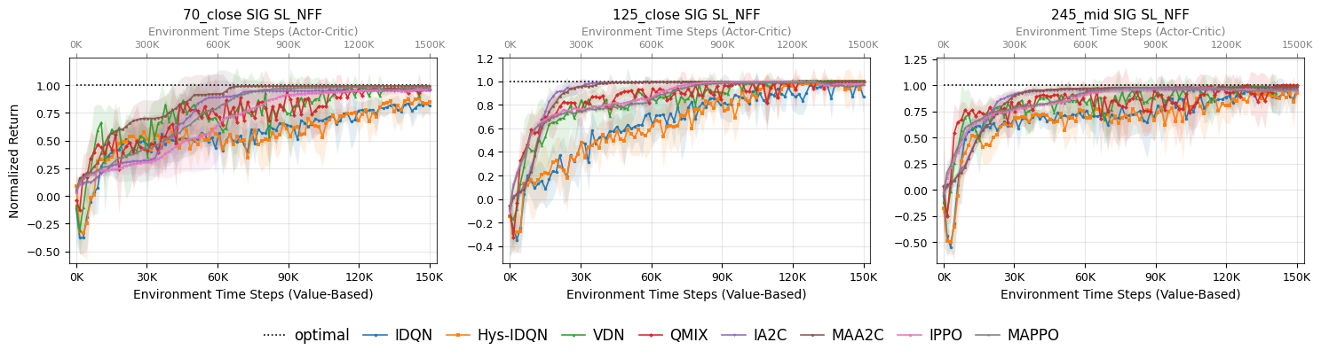
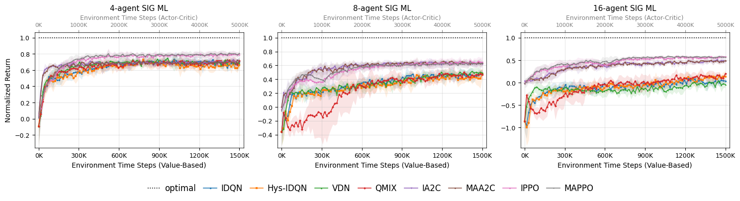
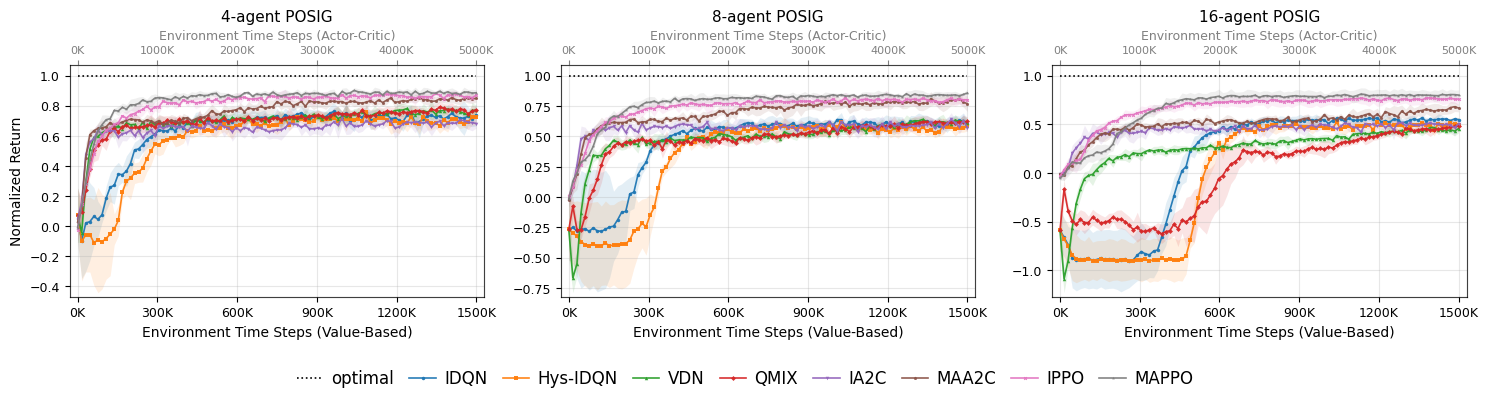
The convergence curves of all algorithms for SIG SL_NFF, SIG ML, and POSIG tasks are shown in Fig. 1, Fig. 2, and Fig. 3, respectively. It can be observed that actor-critic algorithms consistently display stable, monotonic improvements, whereas value-based methods exhibit pronounced oscillations and higher variance. This instability arises because value-based learning repeatedly bootstraps from non-stationary Q-targets, making updates sensitive to short-term reward fluctuations.
The key insights from the POSIG results are as follows:
Despite operating under partial observability, POSIG outperforms or matches SIG ML across all algorithms, with the gains being particularly significant for value-based methods. We hypothesize that the compact local observations in POSIG provide a more effective and scalable representation for learning than the high-dimensional state representation used in SIG ML.
In partially observable environments, the CTDE paradigm benefits actor-critic algorithms but offers diminishing, or even negative, advantages for value-based algorithms as the number of agents increases.
MAPPO achieves the best overall performance across all tasks, whereas IPPO delivers only slightly lower performance while offering superior scalability.
To summarize the findings of Section VII, Table 7 presents a challenge-oriented attribution analysis. Each row corresponds to the introduction of a new MARL challenge through the transition from one learning task to the next and reports the resulting change in average normalized return, measured in percentage points (pp). For each task, we first compute the average normalized return across the eight evaluated algorithms, representing the fraction of the random-to-reference performance gap closed by the algorithms. The performance change is computed as the difference between the average normalized return of the current task and that of the corresponding baseline task. The baseline is the preceding learning task within the same agent-count column, except for the first row and the large-action-space row. For NFIG, the baseline is the optimal performance obtained through exhaustive search. For the large-action-space row, the 8- and 16-agent results are compared with the corresponding 4-agent reference. Negative values indicate performance degradation, while positive values indicate performance improvement.
The results show that non-stationarity and coordination difficulty reduce performance by only 1 percentage point in the four-agent single-topology setting, while introducing multiple decision steps causes a further 1-percentage-point decrease. Increasing the number of agents from four to sixteen results in a 7-percentage-point reduction. In contrast, the transition from SIG SL_FF to SIG ML, which introduces topology diversity and the associated robustness and generalization challenge, causes much larger degradations of 23, 40, and 59 percentage points for the 4-, 8-, and 16-agent settings, respectively. Partial observability does not introduce additional degradation; instead, performance increases by 6, 13, and 28 percentage points in the corresponding settings. Overall, these results identify robustness and generalization across diverse vehicular topologies as the dominant challenge in the proposed benchmark.
| Task | Added MARL challenge | Performance change (pp) | ||
|---|---|---|---|---|
| 3-5 | 4 ag. | 8 ag. | 16 ag. | |
| NFIG | Non-stationarity, coordination | \(-1\) | — | — |
| SIG SL_NFF | Multi-step | \(-1\) | — | — |
| SIG SL_FF | Large action space | — | \(-1\) | \(-7\) |
| SIG ML | Robustness/generalization | \(\mathbf{-23}\) | \(\mathbf{-40}\) | \(\mathbf{-59}\) |
| POSIG | Partial observability | \(+6\) | \(+13\) | \(+28\) |
4pt
8 Conclusion and Future Works↩︎
In this paper, we proposed a series of interference games for RRA in C-V2X networks that enable the systematic isolation and attribution of key MARL challenges. Using this benchmark framework, we evaluated eight classical MARL algorithms and obtained the following key insights:
The most significant challenge in the studied C-V2X environment is not the well-known issues of non-stationarity, coordination, large action space, or partial observability, but rather learning policies that remain effective across diverse vehicular topologies and generalize to unseen ones.
Both value-based and actor-critic algorithms perform well in simplified tasks involving a single fixed topology. However, in more realistic tasks with diverse vehicular topologies, actor-critic algorithms achieve higher performance and exhibit more stable learning behavior.
Among the actor-critic methods, PPO consistently outperforms A2C. Furthermore, incorporating a centralized critic provides only limited benefits for MAPPO over IPPO. Given the scalability limitations of centralized critics, IPPO represents a more practical baseline for large-scale C-V2X RRA.
These findings provide several directions for future research. Although value-based independent learning remains one of the most widely adopted MARL approaches for C-V2X RRA, greater attention should be devoted to actor-critic algorithms because of their superior performance in complex environments. In particular, IPPO offers an attractive balance between performance and scalability.
The comparison among SIG SL, SIG ML, and POSIG reveals that conventional RL algorithms can learn highly effective policies when trained on a single topology, but their performance deteriorates substantially when exposed to a large variety of topologies. The vehicular topology—and consequently the path loss of all links—affects the queue transition dynamics. While topologies remain fixed within an episode, they vary across episodes, making the SIG ML and POSIG environments a continuum of related tasks, each with distinct dynamics. Given the impracticality of learning a separate policy for every possible transition function, it is highly desirable for the learned policy to enable zero-shot transfer, solving both seen and unseen tasks at runtime without additional training.
The superior performance of POSIG relative to SIG ML suggests that more effective state and representation learning mechanisms may play an important role in improving generalization. Advanced architectures such as GNN-based MARL [10], transformer-based MARL, and meta-RL [11] introduce learning mechanisms specifically designed to address challenges such as representation learning, generalization, and rapid adaptation across environments. While these approaches are promising, their effectiveness in C-V2X RRA remains insufficiently understood due to the lack of standardized and controlled benchmark environments. We believe that one important contribution of the proposed benchmark framework is to provide a systematic evaluation platform for such future methods. In particular, the NFIG, SIG SL, and SIG ML tasks provide controlled settings for evaluating coordination, large action space, robustness, and generalization, while POSIG enables investigation of partial observability and representation learning under local observations. By isolating different MARL challenges through progressively more realistic interference games, the proposed benchmark can help future studies identify which challenges are effectively addressed by advanced architectures and which remain unresolved.
It is also important to note that the objective of the proposed benchmark is not to establish deployment-ready scalability to arbitrarily large C-V2X networks, but rather to investigate how key MARL challenges evolve as the number of simultaneously coordinating agents increases. The results consistently show that PPO-based actor-critic methods remain comparatively resilient as the number of simultaneously coordinating agents increases from four to sixteen. While larger-scale studies remain an important direction for future research, particularly under more computationally efficient MARL architectures and training frameworks, the current benchmark provides valuable insights into the relative importance of different MARL challenges and their scaling behavior in C-V2X RRA.
Additionally, the current benchmark adopts controlled observation and agent-availability assumptions, including noise-free observations, instantaneous channel state information, and a fixed set of active agents. These assumptions were intentionally adopted to isolate and quantify the topology-generalization challenge while avoiding confounding factors. Nevertheless, the modular interference-game framework naturally supports controlled extensions to additional robustness dimensions, including noisy observations, delayed information, and missing or inactive agents. By introducing each impairment as a separate task variant while keeping other factors fixed, future studies can systematically quantify the additional difficulty introduced by each impairment and evaluate robustness beyond the topology-generalization challenge considered in this work.
Finally, the conclusions of this paper are based on experiments conducted under the standardized 3GPP TR 36.885 highway evaluation framework. Consequently, the exact numerical results and performance gaps reported here may vary under different deployment scenarios. Nevertheless, the central finding—that robustness and generalization across diverse vehicular topologies constitute the dominant challenge among those considered in this work—is rooted in the fundamental dependence of wireless interference on vehicular topology and is therefore expected to extend beyond the specific highway setting. The current benchmark focuses on topology-induced distribution shifts under a fixed channel model. Other sources of distribution shift, such as changes in propagation environments, channel models, and traffic characteristics, may introduce additional robustness and generalization challenges that warrant further investigation.
9 Hyperparameters↩︎
The hyperparameters used in all experiments are given in Tables 8–11.
| Hyperparameter | IDQN | Hys-IDQN | VDN | QMIX |
|---|---|---|---|---|
| actor/critic hidden dimension (FC) | \(128\) | \(128\) | \(128\) | \(128\) |
| learning rate | \(3 \times 10^{-5}\) | \(3 \times 10^{-5}\) | \(3 \times 10^{-5}\) | \(3 \times 10^{-5}\) |
| mixing network learning rate | - | - | - | \(1 \times 10^{-6}\) |
| hysteretic learning rate | - | \(\alpha{=}1.0, \beta{=}0.2\) | - | - |
| batch size | \(64\) | \(64\) | \(64\) | \(64\) |
| target update (soft) | \(5 \times 10^{-3}\) | \(5 \times 10^{-3}\) | \(5 \times 10^{-3}\) | \(5 \times 10^{-3}\) |
| training episodes | \(50{,}000\) / \(3{,}000\) | \(50{,}000\) / \(3{,}000\) | \(50{,}000\) / \(3{,}000\) | \(50{,}000\) / \(3{,}000\) |
| epsilon anneal steps (linear) | \(40{,}000\) / \(2{,}400\) | \(40{,}000\) / \(2{,}400\) | \(40{,}000\) / \(2{,}400\) | \(40{,}000\) / \(2{,}400\) |
| parameter sharing | False | False | False | False |
| Note: Values shown as \(a / b\) indicate different settings for NFIG / SIG SL respectively. Single values apply to both. | ||||
| Hyperparameter | IA2C | MAA2C | IPPO | MAPPO |
|---|---|---|---|---|
| hidden dimension (FC) | \(128\) | \(128\) | \(128\) | \(128\) |
| actor learning rate (\(\alpha\)) | \(2 \times 10^{-4}\) | \(2 \times 10^{-4}\) | \(4 \times 10^{-4}\) | \(4 \times 10^{-4}\) |
| critic learning rate (\(\beta\)) | \(2 \times 10^{-4}\) | \(2 \times 10^{-4}\) | \(6 \times 10^{-4}\) | \(6 \times 10^{-4}\) |
| batch size | \(8\) | \(8\) | \(256\) | \(256\) |
| mini-batches | - | - | \(4\) | \(4\) |
| target update (soft) | \(0.01\) | \(0.01\) | - | - |
| PPO epochs | - | - | \(10\) | \(10\) |
| entropy coefficient | - | - | \(0.001\) | \(0.001\) |
| training episodes | \(50{,}000\) / \(30{,}000\) | \(50{,}000\) / \(30{,}000\) | \(50{,}000\) / \(30{,}000\) | \(50{,}000\) / \(30{,}000\) |
| parameter sharing | False | False | True | True |
| Note: Values shown as \(a / b\) indicate different settings for NFIG / SIG SL respectively. Single values apply to both. | ||||
| Hyperparameter | IDQN | Hys-IDQN | VDN | QMIX |
|---|---|---|---|---|
| hidden dimension (FC) | \(128\) | \(128\) | \(128\) | \(128\) |
| learning rate | \(10^{-5}\) / \(10^{-6}\) | \(10^{-5}\) / \(10^{-6}\) | \(10^{-5}\) | \(10^{-5}\) |
| mixing network learning rate | - | - | - | \(10^{-6}\) |
| hysteretic learning rate | - | \(\alpha{=}1.0, \beta{=}0.2\) | - | - |
| batch size | \(64\) | \(64\) | \(64\) | \(64\) |
| target update (soft) | \(5 \times 10^{-3}\) | \(5 \times 10^{-3}\) | \(5 \times 10^{-3}\) | \(5 \times 10^{-3}\) |
| training episodes | \(30{,}000\) | \(30{,}000\) | \(30{,}000\) | \(30{,}000\) |
| epsilon anneal steps (linear) | \(24{,}000\) | \(24{,}000\) | \(24{,}000\) | \(24{,}000\) |
| parameter sharing | False | False | False | False |
| Note: Values shown as \(a / b\) indicate different settings for SIG ML / POSIG respectively. Single values apply to both. | ||||
| Hyperparameter | IA2C | MAA2C | IPPO | MAPPO |
|---|---|---|---|---|
| actor/critic hidden dimension (FC) | \(128\) | \(128\) | \(128\) | \(128\) |
| actor learning rate (\(\alpha\)) | \(5 \times 10^{-4}\) | \(5 \times 10^{-4}\) | \(4 \times 10^{-4}\) | \(4 \times 10^{-4}\) |
| critic learning rate (\(\beta\)) | \(5 \times 10^{-4}\) | \(5 \times 10^{-4}\) | \(6 \times 10^{-4}\) | \(6 \times 10^{-4}\) |
| batch size | \(8\) | \(8\) | \(256\) | \(256\) |
| mini-batches | - | - | \(4\) | \(4\) |
| target update (soft) | \(0.01\) | \(0.01\) | - | - |
| PPO epochs | - | - | \(10\) | \(10\) |
| entropy coefficient | - | - | \(0.001\) | \(0.001\) |
| training episodes | \(100{,}000\) | \(100{,}000\) | \(100{,}000\) | \(100{,}000\) |
| parameter sharing | True | True | True | True |
| Note: Values shown as \(a / b\) indicate different settings for SIG ML / POSIG respectively. Single values apply to both. | ||||
References↩︎
\(^{1}\)S. Wang, L. Lei, P. Maheshwari, and S. Bellefeuille are with the College of Engineering, University of Guelph, Guelph, Ontario, Canada (e-mail: leil@uoguelph.ca).↩︎
\(^{2}\)K. Zheng is with the College of Electrical Engineering and Computer Sciences, Ningbo University, Ningbo, 315211, China.↩︎