How to improve the accuracy of semiclassical and quasiclassical dynamics with and without generalized quantum master equations
March 04, 2026
Abstract
Semi- and quasi-classical (SC) theories can handle anharmonic interactions and are thus well-suited to predict atomistic quantum dynamics in condensed phases that encode energy and charge transport, spectroscopic responses, and chemical reactivity. However, SC theories can be computationally expensive and inaccurate. When combined with generalized quantum master equations (GQMEs), the resulting SC-GQMEs can enhance the efficiency and accuracy of SC dynamics. Yet, while the origin of improved efficiency is clear, the mechanism that improves accuracy remains elusive. Even worse, SC-GQMEs can yield unphysical dynamics in challenging parameter regimes—a shortcoming that might be avoided if the mechanism of accuracy improvement were understood. Here, we uncover this mechanism. We leverage short-time analyses to prove that exact, “left-handed” time-derivatives delay the onset of SC inaccuracy, even without the GQME. However, these derivatives are a double-edged sword: while offering greater short-time accuracy, they become unphysical in challenging parameter regimes. Because short-lived SC-GQME kernels combine short-time accuracy with long-time stability, we develop a protocol to unambiguously determine the memory kernel cutoff, even in challenging cases where previous treatments had failed. Our protocol employs only SC calculations and combines self-consistency with mixed-accuracy auxiliary kernels to triangulate a propitious kernel cutoff, yielding SC-GQMEs with greater accuracy than SC theory alone, while remaining physical and accurate over arbitrary times. Our insights into accuracy improvement, identification of when the SC-GQME is advantageous, and kernel cutoff protocol are general and can be expected to apply to complex systems that go beyond simple models.
Accurate quantum dynamics is essential for describing fundamental processes such as charge transfer in solution, energy transport in light-harvesting complexes, and the optical spectra of molecules. When a problem can be written in terms of an open quantum system coupled to a Gaussian environment [1], one can use a variety of numerically exact methods [2]–[15]. However, many physical systems exhibit anharmonic interactions that can engender non-Gaussian statistics, including spin systems [16]–[19], photosynthetic complexes [20], [21], electrochemical interfaces [22]–[24], and technologically relevant semiconductors[25]–[28]. Hence, approximate methods become necessary. Among these, the semi- and quasi-classical hierarchy[29]–[44] stands out due to its compatibility with generally anharmonic ab initio forces and ability to treat non-Gaussian fluctuations. Yet, despite their promise, semiclassics involve uncontrolled approximations that can lead to inaccurate dynamics.
Semi- and quasi-classical (SC) theories treat some degrees of freedom quantum mechanically and others classically, offering a means to approximate quantum dynamics in systems where a fully quantum description is intractable. This family of methods has been instrumental in understanding superconductivity [45], [46], modeling charge transport from first principles[47]–[49], describing complex interactions in spin systems [50]–[52], and simulating linear and non-linear spectroscopies [53]–[66]. However, SC methods are beset by problems, such as violating detailed balance[67]–[70] and creating artificial resonances or shifts in spectroscopic peaks[60], [71]–[75]. Researchers have adopted various strategies to address these challenges. For example, one can incorporate more quantum effects using the path integral formalism [76]–[82] or the quantum-classical Liouville equation [83]–[87], but this generally entails a trade-off between higher accuracy and increased computational cost. Another way is to partition a system’s degrees of freedom into two different categories and treat one set with numerically exact or perturbative approaches and the other set semiclassically [88]–[93], but this generally requires Gaussian environments or exactly solvable Hamiltonian partitions. Finally, one can combine SC theory with generalized quantum master equations (GQME). These SC-GQMEs extract the non-Markovian generator of the dynamics, i.e., the memory kernel, using SC theory, enabling the subsequent solution of the GQME. SC-GQMEs have been shown to provide significant boosts in accuracy and efficiency to SC methods, and have been demonstrated both in [94] and out[95]–[106] of equilibrium, for atomistic systems[107], multi-state problems [108], [109], and even multitime correlation functions for nonlinear spectroscopies [110]. However, fundamental questions remain regarding the source of their improved accuracy, when they are advantageous, and why they sometimes fail. We consider these questions here.
How and when do GQMEs improve SC dynamics? Early work posited that it was the confluence of short-lived memory kernels and the short-time accuracy of SC methods that endowed SC-GQMEs with improved accuracy [98]. However, later work showed that long-lived memory kernels could still improve the accuracy of SC dynamics, and proposed that this improvement arises from exact sampling of bath correlations at time \(t=0\) used to construct the SC-GQME kernel [99]. Building on these insights, Ref. -’ [100] established mathematical requirements for when one should expect the self-consistent extraction of the memory kernel in the SC-GQME to provide either the same or different (not necessarily better) level of accuracy compared to the original SC dynamics. Indeed, it was later shown that the SC-GQME can generate worse dynamics than the original SC approximation, even with unphysical, negative populations, in systems with large energy biases and system-bath coupling[105]. This is a worrying situation because, to date, no diagnostic exists to determine if and when the SC-GQME should be expected to improve SC dynamics. This presents a problem when describing complex processes where exact quantum dynamics become challenging, including energy flow in photosynthetic complexes or charge transport in transition metal oxides, which exhibit strong electronic-nuclear coupling and significant energetic disorder [111]–[113].
Here, we resolve these issues by addressing the following questions:
What is the mechanism of accuracy improvement in the SC-GQME?
What is the role of self-consistency in the SC-GQME?
How can one reliably improve SC dynamics with and without the SC-GQME?
In particular, we leverage a short-time expansion analysis to demonstrate that improved accuracy arises from exact time derivatives on the initial condition that delay the onset of error arising from the SC approximation. This enables us to show that simple numerical integration of these time derivatives yields improved accuracy, even in the absence of the GQME. However, we find that, while offering greater short-time accuracy, these time derivatives can become inaccurate, even unphysical, at long times in challenging parameter regimes. Returning to the SC-GQME, our analysis shows that the self-consistent structure of the SC-GQME is not strictly necessary to improve the accuracy of SC dynamics. Instead, we establish that it can help ensure sum rules, such as population conservation in the calculated nonequilibrium averages of reduced density matrices. By understanding static sampling errors in SC correlation functions, we show that one can impose the same conservation laws with a predictable uniform shift of the time derivatives. Noting, then, that SC-GQMEs are most beneficial when they exhibit short-lived kernels that capitalize on short-time accuracy while circumventing long-time instability of exact time derivative-rotated initial conditions, we propose a new, unambiguous protocol to truncate the memory kernel, even in challenging parameter regimes where previous protocols had failed. Our kernel truncation metric is self-contained and only requires access to the SC dynamics used to construct the SC-GQME kernel. Importantly, our protocol is compatible with advances in sampling initial conditions for atomistic systems[114]–[119], and may be expected to allow for physically meaningful and accurate dynamics that surpass those of SC methods alone. We observe that, with this protocol, the resulting SC-GQME dynamics are always as accurate or more than the direct SC approximation.
1 SC Method and Illustrative Models↩︎
While our conclusions in this work are independent of the choice of SC theory and model, we illustrate our arguments by employing the linearized semiclassical initial value representation (LSC) method [32] as our choice of SC theory to simulate the reduced (spin) density matrix dynamics of the spin-boson model [120]. Specifically, we quantify the accuracy of SC theory and our modifications to it by benchmarking against the population dynamics, \(\langle \sigma_z(t)\rangle\), obtained using the numerically exact, path integral-based time-evolving matrix product operator (TEMPO) approach [121]. In the Supplementary Information (SI) Sec. I, we further test the performance of our ideas with respect to coherence dynamics and other SC methods (see SI Sec. I A and B).
We choose the spin-boson model because it is the paradigmatic open quantum system that illustrates decoherence, dissipation, and thermalization, and can be used to model electron, charge, and spin transfer in the condensed phase[120], [122]. However, our conclusions are broadly applicable to systems in contact with thermal reservoirs, including, e.g., the Frenkel exciton model (see SI Sec. I C). The spin-boson model consists of a central spin connected to a Gaussian thermal environment, \[\hat{H} = (\varepsilon + \hat{V}_B) \hat{\sigma}_z + \Delta \hat{\sigma}_x + \frac{1}{2}\sum_n \big( \hat{p}_n^2 + \omega_n^2 \hat{x}_n^2\big),\] where \(\{ \hat{\sigma}_i \}\) are Pauli matrices, \(\varepsilon\) is spin’s bias, \(\Delta\) is its diabatic coupling, \(\omega_n\), \(\hat{p}_n\), and \(\hat{x}_n\), are the frequency and mass-weighted momenta and positions of the \(n^{\rm th}\) oscillator in the thermal bath, and \(\hat{V}_B = \sum_n c_n\hat{x}_n\) is the bath part of the system-bath coupling, with \(c_n\) being the coupling to the \(n^{\rm th}\) oscillator. The spectral density, \[J(\omega) = \frac{\pi}{2} \sum_n \frac{c_n^2}{\omega_n} \delta\left(\omega - \omega_n\right)\] determines the coupling between the system and bath. For simplicity, we employ an Ohmic spectral density with an exponential cutoff \(J(\omega) = \frac{\pi}{2}\eta \omega e^{-\omega/\omega_c}\), where \(\frac{\pi}{2}\eta = \pi\lambda/\omega_c\), is the Kondo parameter, and \(\lambda = \frac{1}{\pi}\int_0^{\infty}{\rm d}\omega\;J(\omega)/\omega\) is the reorganization energy quantifying the strength of system-bath coupling and \(\omega_c\) is the cutoff frequency that determines how quickly the thermal bath dissipates energy.
Arguably the simplest method in the SC hierarchy, the LSC method [32], [78] is equivalent to truncated Wigner approximation[51], [123], [124] and offers accuracy comparable to mean-field methods such as Ehrenfest theory [125]–[128] . Because LSC contains the least quantum treatment, it offers a hard test for our analysis. LSC encodes quantum mechanics only in the initial and final conditions for measurement and employs classical dynamics to evolve all variables. In Wigner phase space, LSC approximates a quantum correlation function thus: \[\begin{align} \label{lsc-ivr-approx} C_{AB}(t) &= \mathrm{Tr}\{\hat{\rho}_B \hat{A}e^{i\mathcal{L}t}\hat{B}\}\\ &\approx (2\pi)^{-f} \int {\rm d}\boldsymbol{\Gamma}\;(\hat{\rho}_B \hat{A})^W_{ \boldsymbol{\Gamma}}e^{i\mathcal{L}^Wt}B^W_{\boldsymbol{\Gamma}}\\ &= (2\pi)^{-f} \int {\rm d}\boldsymbol{\Gamma}\;(\hat{\rho}_B \hat{A})^W_{ \boldsymbol{\Gamma}}B^W_{\boldsymbol{\Gamma}}(t). \end{align}\tag{1}\] Here, \(f\) is the total number of degrees of freedom (electronic and nuclear), \(\Gamma = \{\mathbf{X}, \mathbf{P}, \mathbf{x}, \mathbf{p} \}\) constitutes the phase space for the subsystem and bath, and \(\mathcal{L}^W\) is the Wigner-transformed [129], [130] quantum Liouvillian, which is equivalent to the classical Poisson bracket, with \(e^{i\mathcal{L}^W t}\) becoming the classical Hamiltonian propagator. To obtain a continuous, Cartesian representation of the spin’s outer product states, \(\{ \ket{j}\bra{k}\} \mapsto \{ \mathbf{X}, \mathbf{P}\}\), the LSC treatment of such open quantum systems employ the Meyer-Miller-Stock-Thoss mapping [131], [132]. We refer the reader to the SI Secs. II A and B for details on exact simulations and LSC simulations, which we propagate using a split-operator algorithm [133].
2 Self-consistent GQMEs↩︎
We start by delineating the anatomy of GQMEs and SC-GQMEs, which necessitates introducing new notation. Here, we provide a table summarizing our notation (see Table ¿tbl:table:table1?).
| \(\mathcal{C}(t)\) | Correlation function |
|---|---|
| \(\mathcal{K}(t)\) | Memory kernel |
| \(\big[\mathcal{C}(t)\big]_{\rm LSC}\) | LSC approximated \(\mathcal{C}(t)\) |
| \(\partial_t^n\big[\mathcal{C}(t)\big]_{\rm LSC}\) | \(n^{\rm th}\) numerical time derivative of \(\big[\mathcal{C}(t)\big]_{\rm LSC}\) |
| \(\big[\dot{\mathcal{C}}^{(nL/nR)}(t)\big]_{\rm LSC}\) | LSC approximated \(n^{\rm th}\) left- or right-handed derivative(s) of \(\mathcal{C}(t)\) |
| \(\big[\mathcal{C}^{(nL/nR)}(t)\big]_{\rm LSC}\) | Integrated \(\big[\dot{\mathcal{C}}^{(nL/nR)}(t)\big]_{\rm LSC}\) |
| \(\big[\dot{\bar{\mathcal{C}}}^{(nL/nR)}(t)\big]_{\rm LSC}\) | Statically shifted \(\big[\dot{\bar{\mathcal{C}}}^{(nL/nR)}(t)\big]_{\rm LSC}\) |
| \(\big[\bar{\mathcal{C}}^{(nL/nR)}(t)\big]_{\rm LSC}\) | Integrated \(\big[\dot{\bar{\mathcal{C}}}^{(nL/nR)}(t)\big]_{\rm LSC}\) |
| \(\mathcal{K}^{(x)}(t)\) | Auxiliary kernel, \(x\in \{ 1, 3b, 3f \}\) |
| Memory kernel constructed from \(\big[\bar{\mathcal{C}}^{nL}(t)\big]_{\rm LSC}\) and its time derivatives |
GQMEs[134]–[136] are low-dimensional equations of motion for a few “interesting” degrees of freedom, say electronic excitations in a molecular aggregate [137], transition dipoles in a spectroscopy experiment [109], [138], [139], density fluctuations in a liquid [140], or electric and thermal currents in materials[141]. One can derive a GQME using projection operator techniques [142], [143], and the choice of projection operator, \(\mathcal{P} = |\boldsymbol{A})(\boldsymbol{A}|\), determines which degrees of freedom one is interested in tracking, \(\{A_j \}\). This procedure yields a Volterra equation for \(\mathcal{C}(t)\), the correlation function or nonequilibrium average of interest: \[\label{mnz} \dot{\mathcal{C}}(t) = \mathcal{C}(t)\dot{\mathcal{C}}(0) - \int^t_0 {\rm d}s \; \mathcal{C}(t-s)\mathcal{K}(s),\tag{2}\] where \(\mathcal{C}(t) = (\boldsymbol{A}|e^{i\mathcal{L}t}|\boldsymbol{A})\), \(\mathcal{L}\) is the Liouvillian for the entire system, and \(\mathcal{K}(t)\) is the memory kernel, which describes the influence of all degrees of freedom not included in \(\{ A_j \}\). The definition of the inner product, \((\mathbf{A}|\hat{\mathcal{O}}|\mathbf{B})\) depends on the definition of the projection operator and should be chosen to ensure the idempotency of the projector, \(\mathcal{P}^2 = \mathcal{P}\), and its complement \(\mathcal{Q} = 1 - \mathcal{P}\). Here, we illustrate our ideas using a definition of the inner product that yields nonequilibrium averages in the electronic subspace of an open quantum system linked to a bosonic reservoir: \((A_j|\mathcal{O} |A_k) \equiv \mathrm{Tr}[\hat{\rho}_B A_j^{\dagger}\mathcal{O}A_k]\), with \(\rho_B A^{\dagger}_k\) encoding the initial condition. In particular, we consider the Argyres-Kelley projector [144], for which \(A_j \in \{\ket{j}\bra{k} \}\) spans the coherences and populations of the discrete subspace, but note that the same conclusions arise when using the population projector[145], for which \(A_j \in \{ \ket{j}\bra{j}\}\) spans only the populations. Nevertheless, our conclusions are general and apply both in and out of equilibrium and for other definitions of the inner product.
The projected propagator, \(e^{i\mathcal{Q}\mathcal{L}t}\), in the memory kernel, \(\mathcal{K}(t) = (\boldsymbol{A}|\left(\mathcal{LQ}\right)e^{i\mathcal{QL}t}\left(\mathcal{QL}\right)|\boldsymbol{A})\) has historically made this quantity difficult to calculate. However, one may invoke the Dyson identity to obtain a self-consistent expansion of the memory kernel [99], [146], \[\label{ksc1} \mathcal{K}(t) = \mathcal{K}^{(1)}(t) + \int^t_0 {\rm d}s \; \mathcal{K}^{(3b)}(t-s)\mathcal{K}(s),\tag{3}\] into two auxiliary kernels \[\begin{align} \tag{4} \mathcal{K}^{(1)}(t) &= (\boldsymbol{A}|\left(\mathcal{LQ}\right) e^{i\mathcal{L}t} \left(\mathcal{QL}\right)|\boldsymbol{A}), \\ \tag{5} \mathcal{K}^{(3b)}(t) &= i(\boldsymbol{A}|\left(\mathcal{LQ}\right) e^{i\mathcal{L}t} |\boldsymbol{A}), \end{align}\] that no longer use the projected propagator. This enables one to use any dynamics solver to obtain \(\mathcal{K}^{(1)}(t)\) and \(\mathcal{K}^{(3b)}(t)\). Evaluating \(\mathcal{K}^{(1)}(t)\) and \(\mathcal{K}^{(3b)}(t)\) using SC dynamics is what constitutes the SC-GQME.
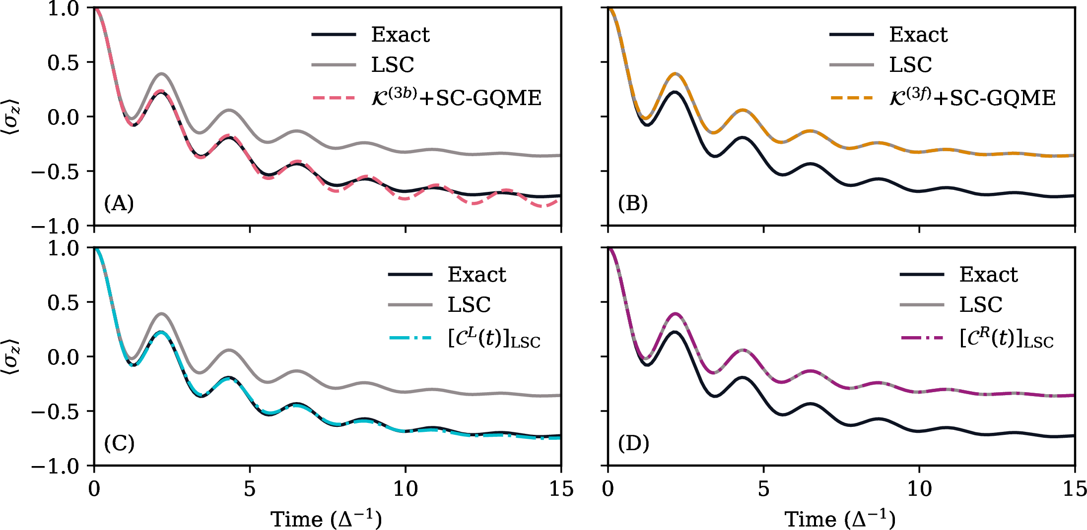
Figure 1: No caption. a — Accuracy improvement in the SC-GQME and its relation to left- and right-handed derivatives. Nonequilibrium population dynamics in the spin–boson model subject to initial condition \(\rho(0) = \rho_B\ket{1}\bra{1}\) with parameters \(\epsilon = \Delta\), \(\beta = 5.0\Delta^{-1}\), \(\omega_c = 2.0\Delta\), \(\eta = 0.2\Delta\) with Ohmic spectral density. Panels compare exact (black) and LSC dynamics (gray) with (A) \(\mathcal{K}^{(3b)}(t)\) as the generator of the SC-GQME, (B) \(\mathcal{K}^{(3f)}(t)\) as the generator of the SC-GQME. Panels (C) and (D) show the dynamics obtained by integrating \(\big[\dot{\mathcal{C}}^L(t)\big]_{\rm LSC}\) and \(\big[\dot{\mathcal{C}}^R(t)\big]_{\rm LSC}\), respectively.
When employing exact quantum dynamics, one can alternatively derive an equally valid self-consistent expansion of the memory kernel [99], \[\label{ksc2} \mathcal{K}(t) = \mathcal{K}^{(1)}(t) + \int^t_0 {\rm d}s \; \mathcal{K}(t-s)\mathcal{K}^{(3f)}(s),\tag{6}\] where, \[\label{k3f} \mathcal{K}^{(3f)}(t) = i(\boldsymbol{A}| e^{i\mathcal{L}t} \left(\mathcal{QL}\right)|\boldsymbol{A}).\tag{7}\] Equations 3 and 6 are equally valid when using numerically exact quantum dynamics to evaluate the auxiliary kernels and yield the same memory kernel and GQME dynamics. However, this equivalence does not generally hold when using approximate dynamics [99]. For example, noting that one can rewrite \(\mathcal{K}^{(1)}(t)\) as a time derivative of \(\mathcal{K}^{(3b)}(t)\) and \(\mathcal{K}^{(3f)}(t)\), i.e., \[\begin{align} \mathcal{K}^{(1)}(t) &= \dot{\mathcal{K}}^{(3b)}(t) - \mathcal{K}^{(3b)}(t)\dot{\mathcal{C}}(0), \\ \mathcal{K}^{(1)}(t) &= \dot{\mathcal{K}}^{(3f)}(t) - \dot{\mathcal{C}}(0)\mathcal{K}^{(3f)}(t), \end{align}\] Ref. -’ [99] showed that adopting \(\mathcal{K}^{(3b)}(t)\) as the generator of the memory kernel yielded a backward SC-GQME with improved dynamics but using \(\mathcal{K}^{(3f)}(t)\) as the generator of the memory kernel resulted in a forward SC-GQME, whose dynamics were as inaccurate as the original SC dynamics (see Fig. 1 (A) and (B)). We provide expressions for all auxiliary kernels in SI Sec. III C.
3 Mechanism for accuracy improvement↩︎
The difference in accuracy improvement afforded by \(\mathcal{K}^{(3b)}(t)\) and \(\mathcal{K}^{(3f)}(t)\) continues to be particularly surprising since the only difference between these auxiliary kernels is the direction in which one applies the Liouvillian operator as the generator of the time derivative, either on the initial condition in Eq. 5 or the final measurement in Eq. 7 . Hence, there exists an asymmetry when taking the analytical derivative on the initial versus final conditions from a semiclassical perspective.
To highlight this asymmetry, we rewrite the auxiliary kernels by explicitly noting whether they invoke right- or left-handed derivatives of \(\mathcal{C}(t)\)—\(\dot{\mathcal{C}}^R(t)\) and \(\dot{\mathcal{C}}^L(t)\), respectively. To obtain such expressions, one substitutes the definition of \(\mathcal{Q}\) into the form of each auxiliary kernel, \[\tag{8} \begin{align} \mathcal{K}^{(1)}(t) = &-\ddot{\mathcal{C}}^{LR}(t) + \dot{\mathcal{C}}(0)\dot{\mathcal{C}}^R(t) + \dot{\mathcal{C}}^L(t)\dot{\mathcal{C}}(0) \nonumber \tag{9} \\ \; &- \dot{\mathcal{C}}(0)\mathcal{C}(t)\dot{\mathcal{C}}(0) \\ \mathcal{K}^{(3b)}(t) = &-\dot{\mathcal{C}}^L(t) + \dot{\mathcal{C}}(0)\mathcal{C}(t) \\ \mathcal{K}^{(3f)}(t) = &-\dot{\mathcal{C}}^R(t) + \mathcal{C}(t)\dot{\mathcal{C}}(0) \end{align}\] where, \[\begin{align} \dot{\mathcal{C}}^L(t) &= -i(\mathcal{L}\boldsymbol{A}|e^{i\mathcal{L}t}|\boldsymbol{A}), \\ \dot{\mathcal{C}}^R(t) &= i(\boldsymbol{A}|e^{i\mathcal{L}t}|\mathcal{L}\boldsymbol{A}), \\ \ddot{\mathcal{C}}^{LR}(t) &= (\mathcal{L}\boldsymbol{A}|e^{i\mathcal{L}t}|\mathcal{L}\boldsymbol{A}). \end{align}\] Because performing a numerical time derivative of \(\mathcal{C}(t)\) is equivalent to taking a single right-handed derivative [100], it appears that the SC-GQME relies on this asymmetry to obtain accuracy improvements. While true for the first right-handed derivative, we show more broadly where this ostensible equivalence holds in Eqs. 11 13 .
3.1 Is self-consistency necessary?↩︎
Given that the only difference in constructing the backward and forward SC-GQMEs is their use of left- versus right-handed time derivatives, respectively, can one obtain similar improvements by directly integrating \(\dot{\mathcal{C}}^L(t)\) versus \(\dot{\mathcal{C}}^R(t)\) to recover \(\mathcal{C}(t)\)? Specifically, one could calculate \(\mathcal{C}(t)\) by integrating the time-derivative, bypassing the self-consistent structure of the SC-GQME altogether, \[\label{integration} \mathcal{C}^{(L/R)}(t) \equiv \mathcal{C}(0) - \int^t_0 {\rm d}s \; \dot{\mathcal{C}}^{(L/R)}(s).\tag{10}\] To pursue this question, we return to the population dynamics in Fig. 1 (A) and (B). Panels (C) and (D) show the results of numerically integrating the LSC approximations to \(\dot{\mathcal{C}}^L(t)\) and \(\dot{\mathcal{C}}^R(t)\) that we used to construct the backward and forward SC-GQMEs, respectively. We provide expressions for these derivatives in SI Sec. III D. The results show that integrating \(\big[\dot{\mathcal{C}}^L(t)\big]_{\rm LSC}\) yields dynamics that closely match the numerically exact dynamics and the improved dynamics afforded by the backward SC-GQME that uses \(\mathcal{K}^{(3b)}(t)\), while integrating \(\big[\dot{\mathcal{C}}^R(t)\big]_{\rm LSC}\) reproduces the original and inaccurate LSC dynamics for \(\langle \sigma_z(t)\rangle\) and the forward SC-GQME dynamics obtained from \(\mathcal{K}^{(3f)}(t)\). Similar improvement extends to observables governed by electronic coherences, such as \(\langle \sigma_x \rangle\) and \(\langle \sigma_y \rangle\), where integrating \(\big[\dot{\mathcal{C}}^L(t)\big]_{\rm LSC}\) consistently maintains agreement with the exact dynamics for a longer period of time compared to the LSC dynamics in line with trends reported for the SC-GQME[106] (see SI Sec. I A) . We thus conclude that self-consistency is not strictly necessary to improve the accuracy of SC dynamics.
Figure 1 raises two intriguing questions. First, how does integrating \(\big[\dot{\mathcal{C}}^L(t)\big]_{\rm LSC}\) produce any accuracy improvement whereas \(\big[\dot{\mathcal{C}}^R(t)\big]_{\rm LSC}\) does not? To answer Q1, we must understand this asymmetry. The following observation also motivates a second question: while both the backward SC-GQME and the numerical integration of \(\big[\dot{\mathcal{C}}^L(t)\big]_{\rm LSC}\) yield predictions with improved accuracy, the two do not exactly agree with each other. So, why do they differ? To apply the SC-GQME in a controlled manner, we must resolve these questions.
3.2 Why does \(\mathcal{C}^R(t)\) not improve accuracy?↩︎
We start with the null result by explaining why \(\big[\dot{\mathcal{C}}_{jk}^R(t)\big]_{\rm LSC}\) yields no improvement. This is because the time-derivative of the LSC-approximated \(\mathcal{C}_{jk}(t)\) equals the LSC-approximated correlation function where the rotation caused by the time derivative (i.e., the action of the Liouvillian on \(A_k\)) is done quantum mechanically, before application of the LSC approximation. This latter expression is the definition of the right-handed derivative, \[\label{eq:lsc-time-derivative} \begin{align} \partial_t[\mathcal{C}_{jk}(t)]_{\rm LSC} &= \int {\rm d}\boldsymbol{\Gamma} \; \left(\hat{\rho}_B A_j\right)^W e^{i\mathcal{L}^Wt} (i\mathcal{L}^W) {A_k}^W, \\ &= \int {\rm d}\boldsymbol{\Gamma} \; \left(\hat{\rho}_B A_j\right)^W e^{i\mathcal{L}^Wt} \left(i\mathcal{L}A_k\right)^W\\ &= [\dot{\mathcal{C}}^{R}_{jk}(t)]_{\rm LSC}, \end{align}\tag{11}\] where \(\partial_t\) denotes the numerical time derivative. Hence, since \(\big[\dot{\mathcal{C}}^R(t)\big]_{\rm LSC} = \partial_t[\mathcal{C}_{jk}(t)]_{\rm LSC}\), its numerical integral cannot produce any accuracy improvement.
We note, however, that right-handed and numerical derivatives are not equivalent to all others—if they were, then the LSC approximation would recover the full quantum dynamics. In fact, there is a critical value \(n^*\)—which depends on the model and the observable—beyond which the (quantum mechanical) right-handed and numerical (SC) derivatives acting on the measured variable cease to agree, \[\label{cond2} \left((i\mathcal{L})^nA_k\right)^W \neq ((i\mathcal{L})^W)^n {A_k}^W,\;\;\;{\rm for\;} n \geq n^*.\tag{12}\] The explanation for this is simple: the two flavors of derivative agree when the application of the Wigner transform on the resulting Liouvillian-rotated operator have no correction terms arising from the Moyal product (see SI Sec. IV A). In the case of the spin-boson (and related energy and charge transfer models), this equivalence holds for the first few derivatives of subsystem operators, \(\{\ket{j}\bra{k} \}\) (see SI Sec. IV A). Hence, one can conclude, \[\label{eq:lsc-equivalence-of-rhd-numerical-derivative} \partial_t[\mathcal{C}_{jk}(t)]_{\rm LSC} = [\dot{\mathcal{C}}^{R}_{jk}(t)]_{\rm LSC}.\tag{13}\] This equivalence breaks down at different orders for different operators. For example, in the spin-boson model, \(n^* = 4\) for \(\sigma_z\), while \(n^* = 3\) for \(\sigma_x\) (see SI Sec. IV B). While one could expect discrepancies to arise in the evolution of these operators at orders beyond \(n^{*}\), the order of accuracy of their correlation functions can be higher, as closure against the initial condition can fortuitously cancel some of the erroneous terms (see SI Sec. IV D).
We now turn to \(\dot{\mathcal{C}}_{jk}^L(t)\). Here, the Liouvillian acts on the initial condition, \(\hat{\rho}_BA_j^{\dagger}\), where we demonstrate that the order of applying the Wigner transformation matters even at the level of the first derivative (see SI Sec. IV C), \[(i\mathcal{L} \hat{\rho}_BA_j)^W \neq i\mathcal{L}^W \left( \hat{\rho}_BA_j\right)^W.\] This implies that, \[\partial_t[\mathcal{C}_{jk}(t)]_{\rm LSC} \neq \dot{\mathcal{C}}^L_{jk}(t).\] This inequality emerges because the Wigner transformation of an operator product does not generally equal the product of the Wigner-transformed operators. Accounting for this distinction has been essential for accurately evaluating quantum correlation functions within semiclassical approaches[100], [130], [147], [148].
Hence, upon integrating \(\dot{\mathcal{C}}^L_{jk}(t)\), one should not expect to recover the original LSC approximation to \(\mathcal{C}_{jk}(t)\). This condition is compatible with earlier work delineating conditions for when the SC-GQME can be expected to give the same level of accuracy as the original SC dynamics[100]. Yet, while this analysis shows why \(\big[\mathcal{C}^{R}(t)\big]_{\rm LSC} = \big[\mathcal{C}(t)\big]_{\rm LSC}\) and \(\big[\mathcal{C}^{L}(t)\big]_{\rm LSC} \neq \big[\mathcal{C}(t)\big]_{\rm LSC}\), it does not explain how employing \(\dot{\mathcal{C}}^L(t)\) leads to improved dynamics.

Figure 2: No caption. a — Schematic of how left-handed derivatives can delay the onset of inaccuracy of semiclassical dynamics. Left: Taylor expansion of a representative correlation function, \(\mathcal{C}(t)\), where \(\chi_n\) represents the \(n^{\text{th}}\) static coefficient. Green checks indicate agreement with the exact static coefficient while an orange (red) diamond suggests minor (major) disagreement with the exact static coefficient. Right: graphical representation of the static coefficients of the same representative correlation function, \(\mathcal{C}(t)\). Top right: the static moments of \(\big[\mathcal{C}^R(t)\big]\) are identical to \(\mathcal{C}(t)\) and have minor disagreement from exact dynamics at \(4^{\rm th}\) order (yellow region). Larger disagreements arise at higher orders (red region). Bottom right: the static moments of \(\big[\mathcal{C}^L(t)\big]\) match the exact quantum dynamics through \(4^{\rm th}\) order, but minor disagreements arise at \(5^{\rm th}\) order.
3.3 Why and how does \(\mathcal{C}^L(t)\) improve accuracy?↩︎
We answer this question by turning to short-time analysis based on Taylor expansions. We distinguish between two types of Taylor expansions, one on a Heisenberg-evolved operator: \[\label{operator95exp} A_k(t) = \sum_{n=0}^{\infty} i^n\frac{\mathcal{L}^nA_k}{n!} t^n,\tag{14}\] and one on the correlation function itself: \[\label{corr95exp} \mathcal{C}_{jk}(t) = \sum_{n=0}^{\infty} i^n\frac{\mathcal{C}^{(n)}_{jk}(0)}{n!} t^n,\tag{15}\] where \(\mathcal{C}^{(n)}_{jk}(0) \equiv \frac{{\rm d}^n}{{\rm d}t^n}\mathcal{C}_{jk}(t)\big|_{t=0}\). The critical concept here is how the accuracy of these short-time expansions changes when one applies the SC approximation directly to \(\mathcal{C}(t)\) versus to versions of the correlation functions where one applies left-handed derivatives.
We consider the Taylor expansion of the SC-approximated \(A_k(t)\) and \(\mathcal{C}(t)\). The LSC approximation to an operator’s evolution takes the form: \[[A_k(t)]_{\rm LSC} = e^{i\mathcal{L}^W t} A_k^W = \sum_{n=0}^{\infty} i^n\frac{(\mathcal{L}^W)^nA_k^W}{n!} t^n.\] In contrast, to recover the exact quantum dynamics of this operator in phase space, one would instead need to apply the Wigner transform to both sides of Eq. 14 , meaning that one instead requires \((\mathcal{L}^nA_k)^W\). While we may expect \((\mathcal{L}^nA_k)^W = (\mathcal{L}^W)^nA_k^W\) for low \(n\), this equality breaks down at a threshold order that depends on the form of \(A_k\) [149]. For example, in the case of \(A_k = \sigma_z\), we have already shown the order at which these start to differ is \(n=4\) (see Eq. 12 and SI Sec. IV B). Naively, this suggests that the LSC approximation to the quantum dynamics of \(\langle \sigma_z(t) \rangle\) is only accurate to \(\mathcal{O}(t^4)\) in a Taylor series in time. However, a serendipitous error cancellation via closure against the initial condition leads some erroneous terms to average out to zero. In the case of population dynamics subject to an initial excitation on site \(1\), the deviation between the exact and LSC dynamics only starts at \(n=6\) order (see SI Sec. IV D).
We now posit that modifying the sequence of exact left-handed versus right-handed derivatives consistent with the LSC approximation in Eq. 15 allows one to obtain different predictions for \(\mathcal{C}(t)\) while still using SC dynamics. Specifically, we hypothesize that incorporating a left-handed derivative into \(\mathcal{C}(t)\), before applying the LSC approximation, can delay the onset of inaccuracy in the LSC dynamics. Indeed, the Taylor expansion for the left-handed version of Eq. 10 takes the form: \[\label{modified95exp} \mathcal{C}^{L}(t) = \mathcal{C}(0)+ \sum_{n=1}^{\infty} i^{n}\frac{\mathcal{C}^{(1|n-1)}(0)}{n!} t^{n},\tag{16}\] where \(\mathcal{C}^{(1|n-1)}_{jk}(0) = \partial_t^{(n-1)}\dot{\mathcal{C}}^{L}(t)\big|_{t=0}\) denotes the quantity obtained by taking an exact quantum mechanical derivative on the initial condition followed by Wigner transformation and all other derivatives as the outcome of the repeated application of \(\mathcal{L}^{W}\) on the final measurement. This modification of derivatives does not change the order at which the operator’s LSC evolution differs from the exact quantum result (see Eq. 12 ). However, it alters the initial condition against which the operator is closed, leading one to conclude that the order of accuracy for the resulting \([\mathcal{C}^{L}(t)]_{\text{LSC}}\) can be changed relative to \([\mathcal{C}(t)]_{\text{LSC}}\) (see schematic in Fig. 2). In the case of population dynamics subject to an initial excitation on site \(1\), this new closure yields greater error cancellation and the deviation between exact and LSC dynamics described by Eq. 16 starts beyond \(n=6\) (see SI Sec. IV D). Hence, our hypothesis is correct: by taking an exact left-handed derivative before Wigner transformation, we have delayed the onset of error from the LSC approximation in the short-time expansion of the correlation function of interest.
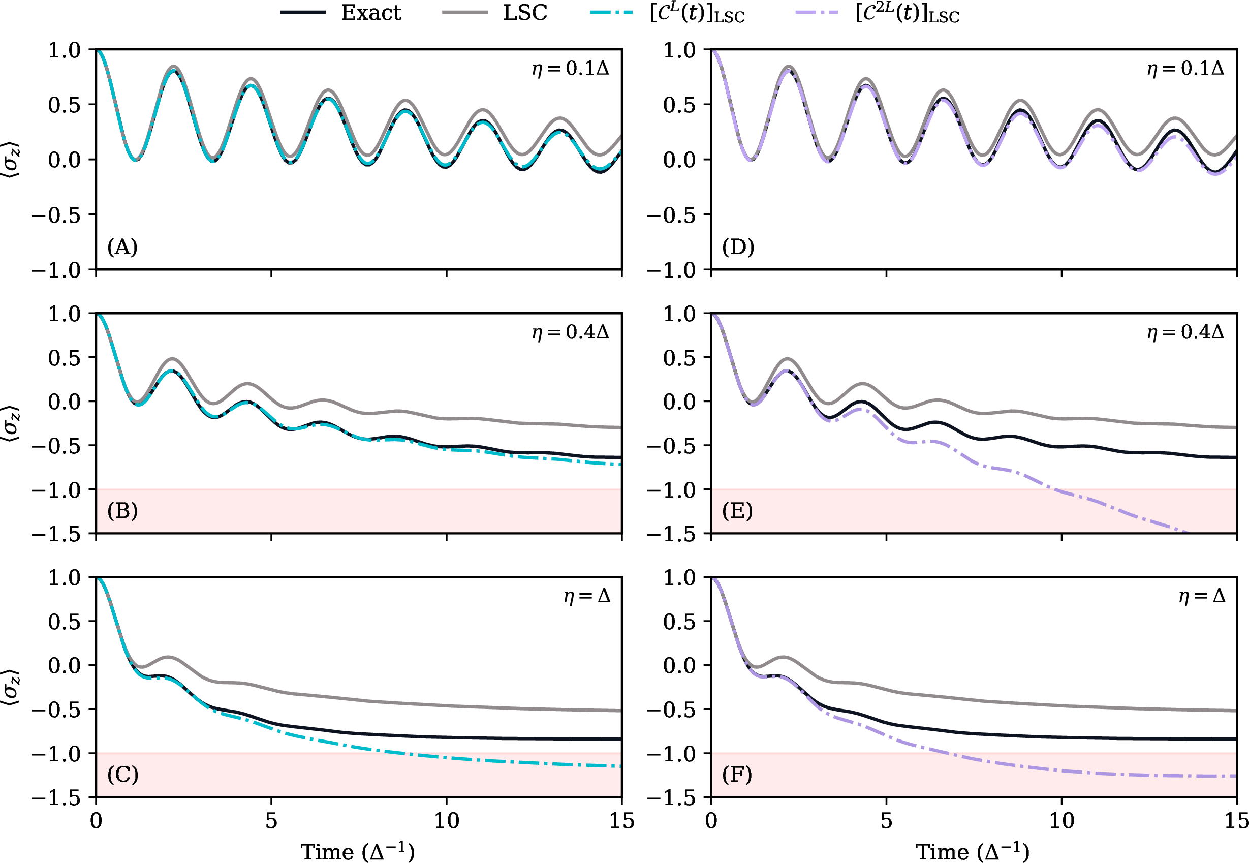
Figure 3: No caption. a — Extent to which left-handed derivatives can improve the accuracy of semiclassical dynamics. Comparison of exact (black) and LSC (gray) population dynamics to integrating \(\big[\mathcal{C}^L(t)\big]_{\rm LSC}\) and \(\big[\mathcal{C}^{2L}(t)\big]\). All panels correspond to the spin–boson model with \(\epsilon = \Delta\), \(\beta = 5.0\Delta^{-1}\), \(\omega_c = \Delta\), an Ohmic spectral density, and varying system–bath coupling, \(\eta\), subject to initial condition \(\rho(0) = \rho_B\ket{1}\bra{1}\). Red shaded regions denote unphysical negative populations.
3.4 When does \(\mathcal{C}^L(t)\) struggle?↩︎
Just as the SC-GQME stops improving SC dynamics in challenging parameter regimes [105], one might expect there to be cases where \(\mathcal{C}^L(t)\) is not sufficient to improve the accuracy of LSC dynamics. These parameter regimes include instances of large bias, which can be expected to exacerbate the difficulties SC methods face in capturing detailed balance, and strong system-bath coupling regimes where the mean-field approximation in LSC is known to fail. For example, in Fig. 3 panels (A), (B), and (C) we show that \([\dot{\mathcal{C}}^{L}(t)]_{\text{LSC}}\) ceases to provide an advantage over \([\mathcal{C}(t)]_{\text{LSC}}\) as a function of increasing system-bath coupling, \(\eta\). Most worrying, however, is the unphysical dynamics of \(\big[\mathcal{C}^{L}(t)\big]_{\rm LSC}\), exhibiting negative populations in the case with the highest coupling, \(\eta = 1\), in panel (C). In such parameter regimes where the one left-handed derivative proves not only insufficient but instead catastrophic, one might wonder if taking additional left-handed derivatives can help. This expectation aligns with our hypothesis that adopting exact left-handed derivatives delays the onset of inaccuracy for the correlation function. Yet, as we show below, one must strike a balance between the delayed onset of inaccuracy in time and the complexity of the initial condition to be sampled, as generated by the repeated action of the exact Liouvillian.
We illustrate this complexity of the initial condition by considering a correlation function starting from the initial condition \(\hat{\rho}_B\ket{1}\bra{1}\), \[\label{eq:noderiv-lsc} [\mathcal{C}_{1B}(t)]_{\rm LSC} = \int {\rm d} \boldsymbol{\Gamma}\;\rho_B^W [\ket{1}\bra{1}]^W B^W_{\boldsymbol{\Gamma}}(t).\tag{17}\] Upon taking the first left-handed derivative, we obtain, \[\label{eq:1LderivLSC} \begin{align} &[\dot{\mathcal{C}}_{1B}^{L}(t)]_{\rm LSC} = -i\int {\rm d} \boldsymbol{\Gamma} \; (\mathcal{L}\rho_B^W \ket{1}\bra{1})^W B^W_{\boldsymbol{\Gamma}}(t)\\ &\quad = \int {\rm d} \boldsymbol{\Gamma}\; \rho_B^W( - \Delta \sigma_y^W +2\xi^W[\ket{1}\bra{1}]^W )B^W_{\boldsymbol{\Gamma}}(t),\\ \end{align}\tag{18}\] where \(\xi^W = \sum_n \frac{-c_n \tanh\left(\frac{\beta \omega_n}{2}\right)p_n}{\omega_n}\). The complexity of Eq. 18 is greater than that of Eq. 17 as one must evaluate correlation functions where the initial condition contains contributions from both coherences (\(\sigma_y^W\)) and populations \((\ket{1}\bra{1})^W\) dressed by bath operators (\(\xi^W\)). Leveraging the intuition that Monte Carlo integration of increasingly complex operators becomes more difficult and computationally demanding, one might imagine that converging these correlation functions subject to these more complex initial conditions takes significantly more sampling than one would require for Eq. 17 . In turn, one can expect that incomplete cancellation of error from finite sampling at the level of Eq. 18 gets amplified in the integrative construction of \(\mathcal{C}^L(t)\) in Eq. 10 . Indeed, \(\sim10^5\) trajectories suffice to converge Eq. 17 , while converging Eq. 18 \(\sim~10^6\) trajectories to achieve similar accuracy when using Eq. 10 .
This complexity only rises further when we pursue the second left-handed derivative,
\[\label{eq:2LderivLSC} \begin{align} [\ddot{\mathcal{C}}_{1B}^{2L}(t)]_{\rm LSC} &= -\int {\rm d} \boldsymbol{\Gamma}\;(\mathcal{L}^2\rho_B^W \ket{1}\bra{1})^W B^W_{\boldsymbol{\Gamma}}(t) \\ &= -\int {\rm d} \boldsymbol{\Gamma}\; \rho_B^W \left[ 2\Delta^2 \sigma_z^W - 2\Delta (\varepsilon + V_B^W) \sigma_x^W + 2\Delta\xi^W \sigma_y^W + 2(\varphi^W - \zeta^W)(\ket{1}\bra{1})^W \right] B^W_{\boldsymbol{\Gamma}}(t). \end{align}\tag{19}\]
Here \(\ddot{\mathcal{C}}^{2L}(t) = -(\mathcal{L}^2\mathbf{A}|e^{i\mathcal{L}t}|\mathbf{A})\), \(V_B^W = \sum_n c_n x_n\), \(\varphi^W = \sum_n c_n \omega_n \tanh(\beta\omega_n/2) x_n\), and \(\zeta^W = 2 (\xi^W)^2 - \sum_n c_n^2 \frac{ \tanh\left(\beta \omega_n/2\right)}{\omega_n}\). Equation 19 poses a monumental challenge to converge, requiring \(\sim 10^7-10^8\) trajectories. Recovering \(\mathcal{C}(t)\) from its second time derivative simply requires double integration, \[\label{double-int} \mathcal{C}^{2L}(t) = \mathcal{C}(0) + \int_0^t {\rm d} s_1 \; \int_0^{s_1} {\rm d}s_2 \; \ddot{\mathcal{C}}^{2L}(s_2).\tag{20}\] Starting with an easy parameter regime, Fig. 3 (A) and (D) show that \(\big[\mathcal{C}^{L}(t)\big]_{\rm LSC}\) in Eq. 10 yields a more accurate result at long times than \(\big[\mathcal{C}^{2L}(t)\big]_{\rm LSC}\) in Eq. 20 —despite our expectation that the second left-handed derivative should provide greater accuracy. This small but significant disagreement illustrates the difficulty of striking a balance between increased accuracy at short times and the much higher computational cost of converging the second left-handed derivative.
Despite the greater complexity of the second left-handed derivative, one might envision parameter regimes where the first derivative struggles but the second derivative can delay the onset of inaccuracy. Figure 3 (E) and (F) focus on stronger system-bath coupling, which is challenging to SC theories. Consistent with the mechanism of short-time accuracy that we have outlined, \([\mathcal{C}^{L}(t)]_{\rm LSC}\) in (C) offers a short-time improvement over \([\mathcal{C}(t)]_{\rm LSC}\), but deviates from the exact result, even turning unphysical at long times. As hypothesized, \(\big[\mathcal{C}^{2L}(t)\big]_{\rm LSC}\) can offer greater short-time accuracy than \(\big[\mathcal{C}^{L}(t)\big]_{\rm LSC}\) in (F), but ultimately falls prey to long-time instability in both (E) and (F). These results suggest that although first and second left-handed derivatives progressively improve short-time accuracy—with diminishing gains—both approaches ultimately exhibit long-time instability in challenging parameter regimes.
3.5 Summary↩︎
Our above analysis establishes a framework that elucidates how to improve the accuracy of SC dynamics via left-handed derivatives. We show that exact (left-handed) derivatives acting on the initial condition before transforming into SC phase space delay the onset of inaccuracy in short-time SC dynamics, providing a concrete answer to Q1, even if long-time inaccuracy can become worse. While one can, in principle, employ any number of analytical derivatives on the initial condition to further delay inaccuracies, this approach is analytically demanding, generally inaccessible unless one has access to an explicit Liouvillian, and poses a significant computational challenge. However, SC-GQMEs may provide an advantage over direct integration of these left-handed derivatives. This is because a GQME’s memory kernel may decay on fast timescales—perhaps faster than the onset of the instability in the left-handed derivatives. In such cases, the SC-GQME can benefit from the enhanced short-time accuracy afforded by the left-handed derivatives while offering a path to construct well-behaved and improved dynamics over all time. Hence, we turn back to the SC-GQME to uncover how it operates and determine whether it works at all differently from simply integrating left-handed derivatives.
4 Apparent differences, conservation laws, & sampling errors↩︎
While it appears that the SC-GQME improves the accuracy of LSC dynamics by leveraging the left-handed derivative \(\dot{\mathcal{C}}^{L}(t)\) in \(\mathcal{K}^{(1)}(t)\) and \(\mathcal{K}^{(3b)}(t)\) (see Eq. 4 and 5 ), Fig. 1 (A) and (C) demonstrate that predictions from the SC-GQME do not exactly match predictions from \([\mathcal{C}^L(t)]_{\rm LSC}\) , especially at long times, despite both yielding improved accuracy. This discrepancy motivates Q2 and implies that the SC-GQME, perhaps through its self-consistent construction of the memory kernel, is doing something different than simply integrating \(\big[\dot{\mathcal{C}}^L(t)\big]_{\rm LSC}\). Motivated by this insight, we ask how the SC-GQME and \(\big[\mathcal{C}^{L}(t)\big]_{\rm LSC}\) differ for alternative metrics, including conservation laws.
To address Q2, we consider the extent to which \(\big[\mathcal{C}^{L}(t)\big]_{\rm LSC}\) and the SC-GQME conserve probability, \(h\), in the electronic subsystem. To illustrate this point, we describe the time-dependence of \(h\) using matrix elements of \(\dot{\mathcal{C}}^L(t)\). Specifically, we consider the matrix elements of \(\dot{\mathcal{C}}^L(t)\) that correspond to initializing an excitation in state \(\ket{1}\bra{1}\) and measuring the excitation in site \(\ket{1}\bra{1}\) and \(\ket{2}\bra{2}\), \[\frac{{\rm d}h^L}{{\rm d}t} = \dot{\mathcal{C}}^L_{11}(t) + \dot{\mathcal{C}}^L_{12}(t),\] In the spin-boson model, exact quantum dynamics trivially satisfy this conservation law, \[\begin{align} \begin{aligned} \frac{{\rm d}h^L}{{\rm d}t} &= -\Delta\mathrm{Tr}\left\{\hat{\rho}_B \hat{\sigma}_y\right\} -i\mathrm{Tr}\{[\hat{V}_B, \hat{\rho}_B] \ket{1}\bra{1}\} = 0. \end{aligned} \end{align}\] However, under the LSC approximation, finite sampling of the initial conditions can cause this condition to no longer be strictly satisfied, \[\begin{align} \begin{aligned} \label{conserve} \frac{{\rm d}h^{L}_{\rm LSC}}{{\rm d}t} &= -\Delta\int {\rm d}\boldsymbol{\Gamma} \; \rho_B^W \sigma_y^W + 2 \int {\rm d}\boldsymbol{\Gamma} \; \xi^W \rho_B^W [\ket{1}\bra{1}]^W\approx 0. \end{aligned} \end{align}\tag{21}\] As the right-hand side of Eq. 21 is calculated from sampling of initial conditions and is independent of the generator of dynamics, it remains a constant through time. Therefore, one would expect the total population to change linearly when integrating \(\big[\dot{\mathcal{C}}^L(t)\big]_{\rm LSC}\). As such, when one samples \(\big[\dot{\mathcal{C}}^L(t)\big]_{\rm LSC}\) and integrates it using Eq. 10 , one should not expect to conserve the total electronic population to high precision, i.e., it should not obey the probability conservation law.
This static error biases the entire LSC correlation function and is magnified upon numerical integration. If this insight is correct, by removing the zero-time bias uniformly across time and instead replacing the zero-time value by either the analytical answer or a highly converged static calculation, \[\label{reference} \begin{align} \dot{\bar{\mathcal{C}}}^{L}(t) &= \dot{\mathcal{C}}^{L}(t) - \dot{\mathcal{C}}^{L}(0) + \dot{\mathcal{C}}^{\rm ref}(0),\\ \ddot{\bar{\mathcal{C}}}^{2L}(t) &= \ddot{\mathcal{C}}^{2L}(t) - \ddot{\mathcal{C}}^{2L}(0) + \ddot{\mathcal{C}}^{\rm ref}(0), \end{align}\tag{22}\] one should conserve population upon numerical integration of the left-handed derivatives. Figure 4 demonstrates this to be true. Thus, the numerically integrated \(\big[\mathcal{C}^L(t)\big]_{\rm LSC}\) fails to conserve population because finite sampling of its initial conditions leave a residual constant bias in the correlation function—a problem that is easy to resolve with the simple shift in Eq. 22 —rather than from any deficiency in the underlying SC methodology.
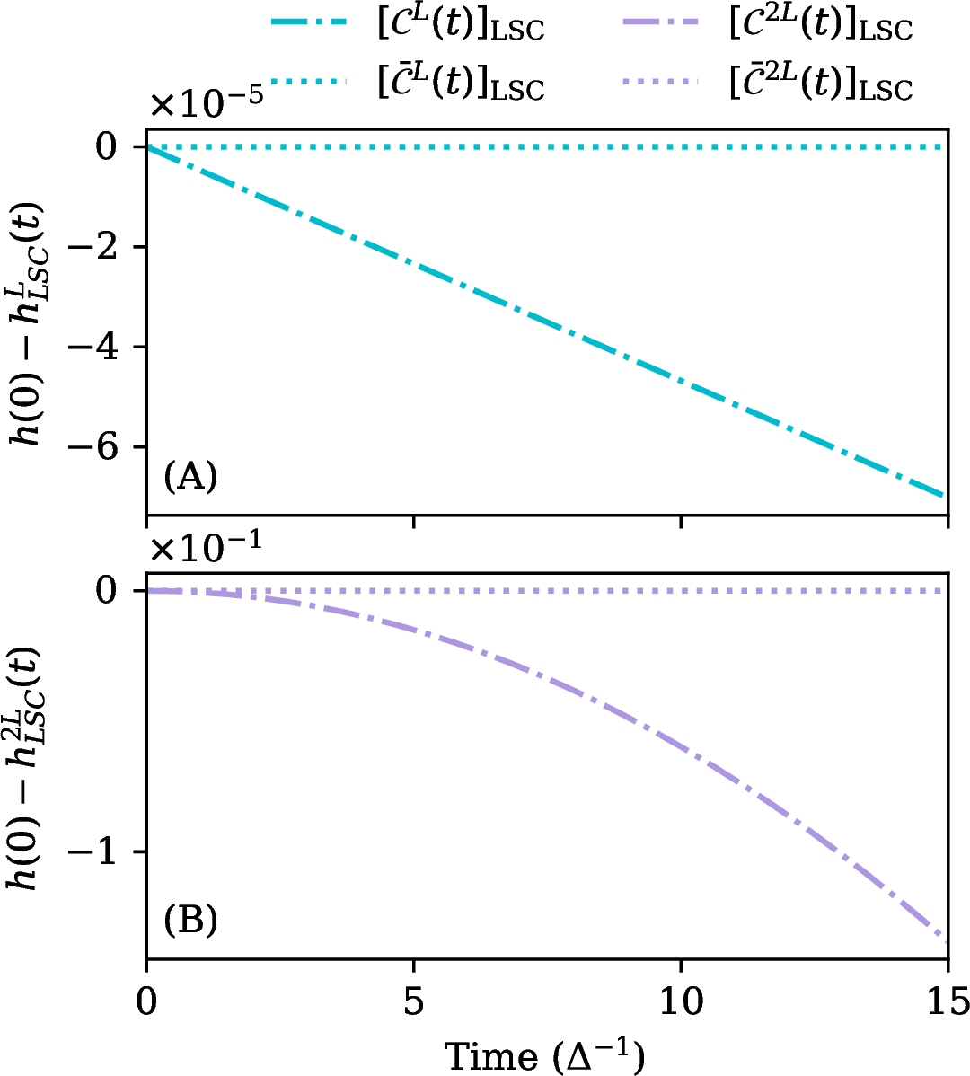
Figure 4: No caption. a — A simple shift allows left-handed derivatives to conserve population. Conservation of total population, \(h\), in (A) \(\big[\mathcal{C}^L(t)\big]_{\rm LSC}\) versus \(\big[\bar{\mathcal{C}}^L(t)\big]_{\rm LSC}\) and (B) \(\big[\mathcal{C}^{2L}(t)\big]_{\rm LSC}\) versus \(\big[\bar{\mathcal{C}}^{2L}(t)\big]_{\rm LSC}\) for a spin-boson model with parameters \(\epsilon = \Delta\), \(\beta = 5.0\Delta^{-1}\), \(\omega_c = 2.0\Delta\), \(\eta = 0.2\Delta\) subject to initial condition \(\rho(0) = \rho_B\ket{1}\bra{1}\).
Interestingly, the current formulation of the SC-GQME preserves the total population, \(h\), for the Argyres-Kelley and population-based projectors in spin-boson model-like problems. However, this is a fortuitous accident arising from the structure of \(\dot{\mathcal{C}}(0)\) and its action in the auxiliary kernels for these projectors, respectively (see SI Sec. V). While we encounter conservation of total population for the chosen projectors in this work, by choosing a different projector—for example, one that projects onto a single population—one no longer guarantees conservation of total population, which can lead to inaccurate descriptions of the dynamics [104]. Nevertheless, applying the same shift of the left-handed derivative can minimize sampling error and ensure total population conserving dynamics (see SI Sec. V E). Moreover, as previous studies [100] have proven, if one constructs a memory using a correlation function and its (commensurably accurate) time derivatives, one must predict the same correlation function from the SC-GQME. Thus, if one builds the memory kernel using only the corrected \(\big[\bar{\mathcal{C}}^L(t)\big]_{\rm LSC}\), which preserves population, and its time derivatives, the SC-GQME must return the same population-conserving dynamics observed in \(\big[\bar{\mathcal{C}}^L(t)\big]_{\rm LSC}\). Figure 5 verifies this fact, with \(\big[\bar{\mathcal{C}}^L(t)\big]_{\rm LSC}\) matching the dynamics of the SC-GQME whose memory kernel we built using \(\big[\bar{\mathcal{C}}^L(t)\big]_{\rm LSC}\) and its time derivatives within \(0.01\%\) error. Figure 5 also reveals that the traditional SC-GQME (labeled ‘SC-GQME’), which uses mixed (0\(^{\rm th}\) and \(1^{\rm st}\)) left-handed derivatives to construct the auxiliary kernels, mixes two levels of accuracy and thus yields similar (albeit not the same) dynamics as the SC-GQME built consistently from the left-handed derivative \(\big[\bar{\mathcal{C}}^{L}(t)\big]_{\rm LSC}\) and its time-derivatives.
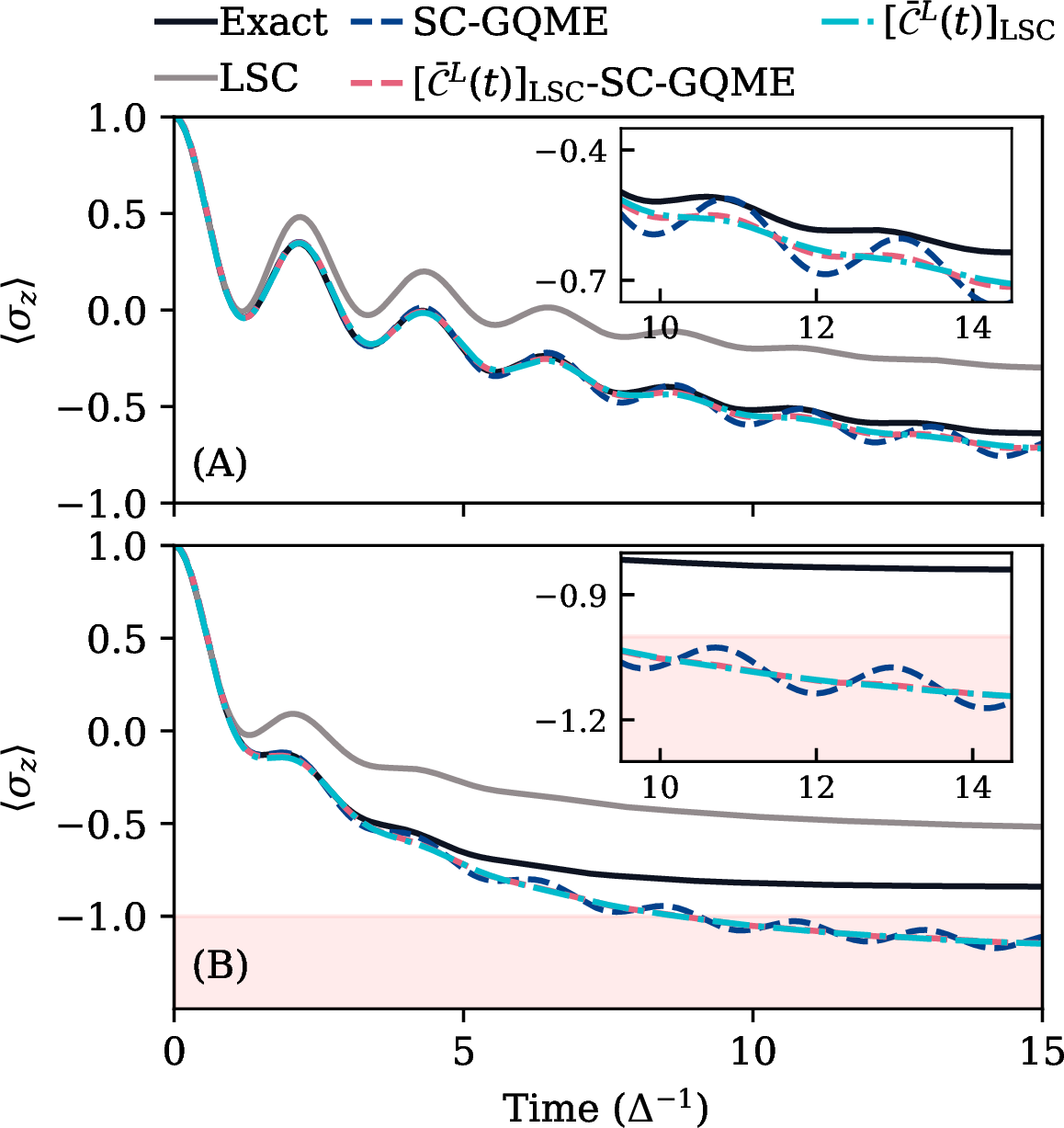
Figure 5: No caption. a — Resolving apparent discrepancies between the SC-GQME and the left-handed derivative. Nonequilibrium population dynamics for the spin-boson model with \(\epsilon = \Delta\), \(\beta = 5.0\Delta^{-1}\), \(\omega_c =\Delta\), an Ohmic spectral density, and subject to initial condition \(\rho(0) = \rho_B\ket{1}\bra{1}\). (A) \(\eta = 0.4\Delta\). (B) \(\eta = \Delta\). Red shaded regions denote nonphysical negative populations. Note that the dynamics obtained from the single-accuracy SC-GQME built on the shifted left-handed derivative, \(\big[\bar{\mathcal{C}}^L(t)\big]_{{\rm LSC}}\)-SC-GQME (dashed cyan line), and the direct integration of \(\big[\bar{\mathcal{C}}^L(t)\big]_{{\rm LSC}}\) (dashed red line) agree, in contrast to the more strongly oscillatory dynamics predicted with the traditional SC-GQME (dashed dark blue line), which is built on mixed-accuracy inputs to the auxiliary kernels. Use of single-accuracy constructions validates the use of equivalence proofs[99], [100] for GQME dynamics.
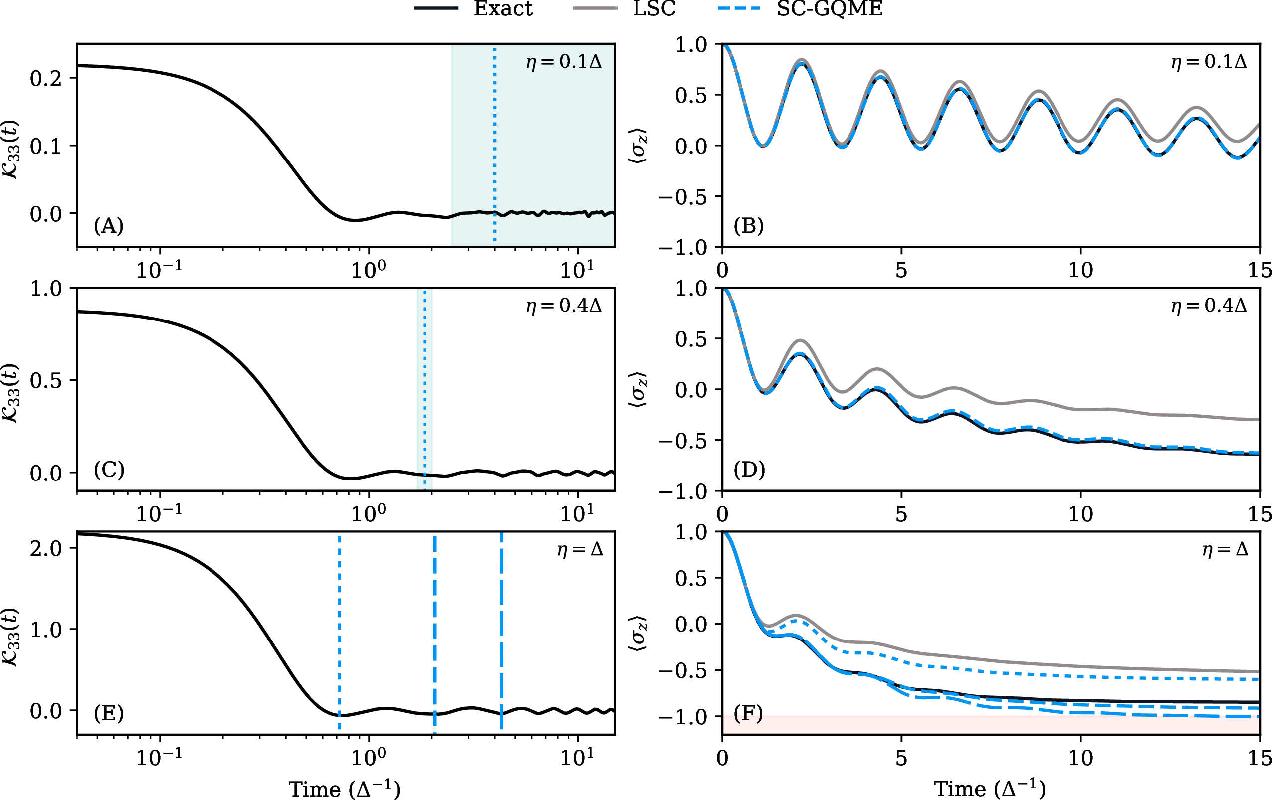
Figure 6: No caption. a — Vanishing “plateaus of stability" complicate the choice of the memory kernel truncation time, \(\boldsymbol{\tau_{\mathcal{K}}}\). Memory kernel elements (left) and nonequilibrium population dynamics (right) for the spin-boson model with \(\epsilon = \Delta\), \(\beta = 5.0\Delta^{-1}\), \(\omega_c = \Delta\), as a function of increasing system-bath coupling, \(\eta\), with an Ohmic spectral density, and subject to initial condition \(\rho(0) = \rho_B\ket{1}\bra{1}\). Green shaded regions indicate the plateau of stability in (A) and (C), and vertical dotted lines correspond to proposed memory kernel cutoffs, \(\tau_{\mathcal{K}}\). Memory cutoffs chosen within this region yield accurate population dynamics shown in (B) and (D). For strong system–bath coupling, the plateau of stability vanishes. Truncation at different times (blue dashed lines in (E)) generate population dynamics (F) with differing long-time limits. Red shaded regions denote unphysical, negative populations.
In summary, we demonstrate that dynamics predicted from integrating \(\big[\dot{\mathcal{C}}^L(t)\big]_{\rm LSC}\) and the SC-GQME differ due to the preservation of conservation laws. We find that the source of this error was a time-independent sampling bias that numerical integration amplifies when obtaining \(\big[\mathcal{C}^{L}(t)\big]_{\rm LSC}\) from \(\big[\dot{\mathcal{C}}^{L}(t)\big]_{\rm LSC}\) or \(\big[\mathcal{C}^{2L}(t)\big]_{\rm LSC}\) from \(\big[\ddot{\mathcal{C}}^{2L}(t)\big]_{\rm LSC}\). We show that we could fix this problem easily by shifting \(\big[\dot{\mathcal{C}}^L(t)\big]_{\rm LSC}\) and \(\big[\ddot{\mathcal{C}}^{2L}(t)\big]_{\rm LSC}\) by the appropriate reference constants, as given by Eqs. 22 . Use of these corrected left-handed derivatives, \(\big[\dot{\bar{\mathcal{C}}}^L(t)\big]_{\rm LSC}\) and \(\big[\ddot{\bar{\mathcal{C}}}^{2L}(t)\big]_{\rm LSC}\), leads to internally consistent integrated and SC-GQME dynamics that conserve population. Finally, our work reveals that employing the same level of left-handed derivatives in the construction of the auxiliary kernels—in contrast to the mixed-accuracy objects relying on different numbers of left-handed derivatives employed in previous versions of the SC-GQME—ensures the internal consistency of the SC-GQME dynamics. Together, these observations allow one to answer Q2 and clarify the role of self-consistency in SC-GQME. The self-consistent structure of the SC-GQME preserves conservation laws when constructed with mixed-accuracy or biased auxiliary kernels. However, the self-consistency neither improves nor impairs the SC-GQME relative to integrating a shifted left-handed derivative (which obeys conservation of population), provided that the auxiliary kernels are constructed from the same number of correspondingly shifted left-handed derivatives.
5 When is the SC-GQME advantageous?↩︎
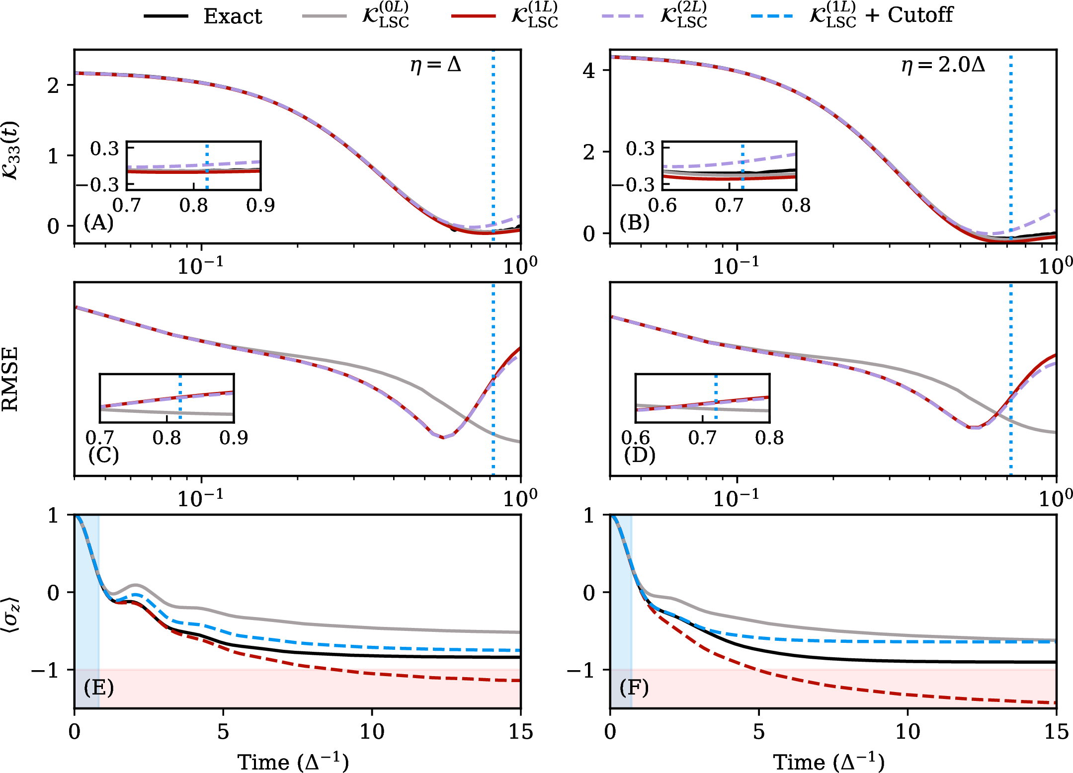
Figure 7: No caption. a — Our RMSE protocol determines optimal cutoff times \(\tau_M\), even in challenging parameter regimes. Single-accuracy memory kernel elements constructed from various numbers of left-handed derivatives (A-B), RMSE of the SC-GQME dynamics with respect to the bare LSC dynamics as a function of proposed kernel truncation time \(\tau_M\) (C-D), and nonequilibrium population dynamics (E-F) for the spin-boson model with \(\epsilon = \Delta\), \(\beta = 5.0\Delta^{-1}\), \(\omega_c = \Delta\), as a function of increasing system-bath coupling, \(\eta\), with an Ohmic spectral density, and subject to initial condition \(\rho(0) = \rho_B\ket{1}\bra{1}\). We choose \(\tau_M\) as the time when the RMSE of \(\mathcal{K}_{\rm{LSC}}^{(1L)}\) (solid red line) and \(\mathcal{K}_{\rm{LSC}}^{(2L)}\) (dashed purple line) start to deviate (dashed blue line). Memory truncation times: \(\tau_M = 0.83\) in (C) and \(\tau_M = 0.72\) (D). (Insets): Enlarged view of the memory kernels (A-B) and RMSE (C-D) around \(\tau_M\). (E-F) Note that the resulting population dynamics from \(\mathcal{K}^{\rm{LSC}}_{1L}\) with memory truncation (dashed blue) are always better than the direct LSC approximation (gray) while avoiding the unphysical behavior evident at long times when using the SC-GQME without (dashed red) memory truncation. The shaded blue region highlights the time up to \(\tau_M\). Red shaded regions denote nonphysical negative populations.
Until now, we have seen that the SC-GQME appears to offer the same level of accuracy as \(\bar{\mathcal{C}}^{L}(t)\). However, we have not yet exploited one of the central benefits of the GQME: when appropriately designed, a GQME’s \(\mathcal{K}(t)\) decays faster (at \(\tau_{\mathcal{K}}\)) than \(\mathcal{C}(t)\) (at \(\tau_C\)). In such cases, one only needs to simulate \(\mathcal{C}(t)\) for short times to construct \(\mathcal{K}(t)\), which then enables one to generate GQME dynamics over arbitrary times at comparatively trivial computational cost. When \(\tau_{\mathcal{K}} \ll \tau_C\), the reduction in the computational cost can reach multiple orders of magnitude [150]–[152]. Beyond this efficiency boost, a short-lived memory kernel can have a second benefit in SC-GQMEs: that \(\big[\bar{\mathcal{C}}^{L}\big]_{\rm LSC}\) and \(\big[\bar{\mathcal{C}}^{2L}\big]_{\rm LSC}\) may be able to offer improved accuracy over \(t \sim \tau_{\mathcal{K}}\) before their accuracy degrades for \(t > \tau_\mathcal{K}\), allowing one to avoid the long-time instabilities evident in Fig 3 (E) and (F). Under these conditions, the SC-GQME may offer improved accuracy, even for parameter regimes where the single and double integration of \(\big[\dot{\bar{\mathcal{C}}}^{L}(t)\big]_{\rm LSC}\) and \(\big[\ddot{\bar{\mathcal{C}}}^{2L}(t)\big]_{\rm LSC}\) would be expected to fail. We demonstrate this below.
5.1 Difficulties of choosing \(\tau_M\)↩︎
In well-behaved dissipative problems, the memory kernel decays to \(0\), allowing one to set an upper bound on the convolution integral in Eq. 2 equal to the memory lifetime, \(\tau_M\), for \(t \geq \tau_M\). This protocol accurately recovers the correlation function \(\mathcal{C}(t)\). Early implementations of the GQME that employed exact solvers for impurity models routinely showed that their GQME dynamics converged with increasing cutoff time, \(\tau_M\) [153]–[155]. This type of analysis also allowed researchers to identify \(\tau_M\) in SC-GQMEs [97], [98]. However, subsequent work showed that memory kernels exhibit high-frequency oscillations when the spectral density of the system spans a wide energetic breadth, making it difficult to identify its decay timescale [99]. Further, the limited accuracy of SC methods can result in memory kernels that do not decay fully [99], [101]. To resolve this ambiguity, Ref. -’ [99] proposed the idea of a “plateau of stability”, corresponding to the range of time during which truncating the memory kernel ceases to influence the SC-GQME dynamics. In practice, one determines \(\tau_M\) as any point within this plateau of stability. Unfortunately, these same studies demonstrated that the size of this plateau of stability depends on the parameter regime [94], [99]. Even worse, in some parameter regimes, this plateau of stability may not even exist [94], [99], [101], [105]. Thus, in challenging parameter regimes, choosing \(\tau_M\) via a disappearing plateau of stability becomes ambiguous at best and impossible at worst.
Figure 6 illustrates how the plateau of stability becomes narrower and even disappears as the parameter regime becomes more challenging to LSC—in this case, as \(\eta\) increases. Despite this difficulty, the smoothness of the SC kernels in Fig. 6 (E) enables us to serendipitously choose a good \(\tau_M\) value (i.e., one that leads to SC-GQME dynamics that closely match the exact benchmark) by picking the second dip of the memory kernel. But, why not pick any point after this? Doing so yields suboptimal—even unphysical—dynamics. The situation worsens when the physical problem involves broader spectral densities, e.g., of a Debye form. In such cases, the resulting SC memory kernels display high-frequency noise [99] that, while globally innocuous, makes it difficult to visually identify when the memory kernel has decayed, revealing the need for an automated method, such as that of plateau of stability identification. Yet, this plateau disappears as the coupling grows, making it clear that a more general method is required.
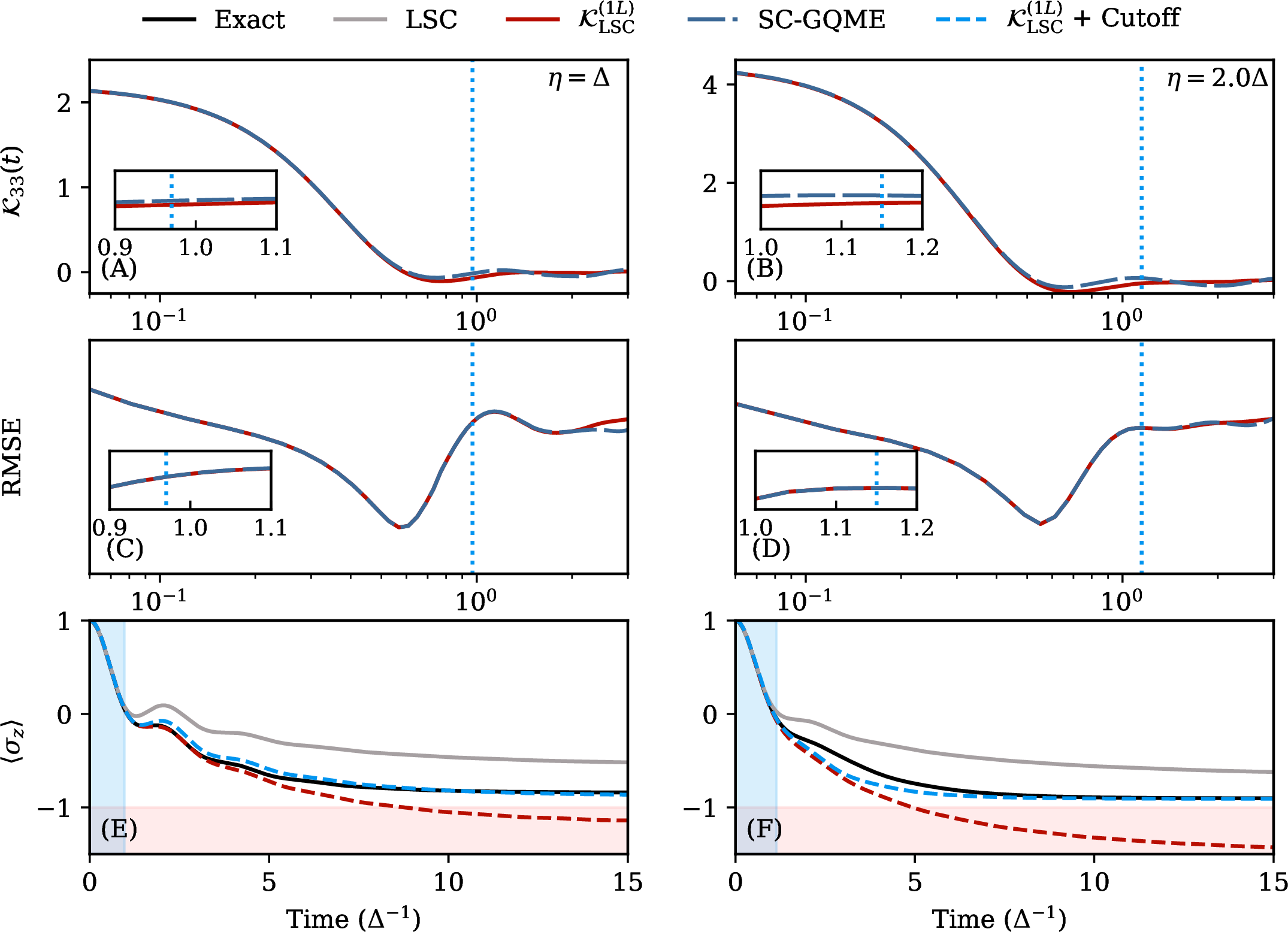
Figure 8: No caption. a — Our RMSE protocol affords even greater accuracy when combined with mixed-accuracy kernels. Here, we report analogous results to Fig. 7 with the main difference being that we compare single-accuracy and mixed-accuracy constructions of the memory kernels. That is, we construct \(\mathcal{K}^{(1L)}_{\rm LSC}(t)\) from single-accuracy auxiliary kernels and \(\mathcal{K}(t)\) from the SC-GQME using mixed-accuracy auxiliary kernels defined in Eq. 8 . Memory truncation times: \(\tau_M = 0.97\) in (C) and \(\tau_M = 1.15\) (D). Particularly noteworthy in (E-F) is the closer agreement to the numerically exact population dynamics (black line) of \(\mathcal{K}^{(1L)}_{\rm LSC}(t)\) coupled with our proposed RMSE-based memory truncation protocol.
5.2 Triangulating accuracy limits↩︎
Figure 6 reveals a major challenge for the SC-GQME: when the plateau of stability disappears, how does one choose a favorable \(\tau_M\) without prior knowledge of the exact dynamics? To answer this question, previous work [103] has attempted to address this challenge by proposing closures that combine auxiliary kernels of mixed accuracy to stabilize the long-time behavior of the memory kernel and avoid the ambiguities illustrated in Fig. 6. While these closures consistently exhibit a plateau of stability and provide an unambiguous truncation time, memory truncation within this framework can still produce unphysical long-time dynamics under strong system-bath coupling (see SI Sec. VI C). Here, we take a fundamentally different approach to address Q3: rather than modifying the construction of the memory kernel, we leverage our understanding of the short-time dynamics to identity the optimal cutoff time for a memory kernel, even one without a plateau of stability, allowing us to optimize accuracy while always providing physically meaningful dynamics. We know, for example, how to ensure that the SC-GQME retains the same accuracy as the dynamics from which we build its memory kernel. That is, if one uses \([\mathcal{C}(t)]_{\rm LSC}\) and its numerical time derivatives, \(\partial_t[\mathcal{C}(t)]_{\rm LSC}\) and \(\partial_t^{2}[\mathcal{C}(t)]_{\rm LSC}\), to construct \(\mathcal{K}(t) \equiv \mathcal{K}_{\rm LSC}^{(0L)}(t)\), the resulting SC-GQME dynamics are identical to \([\mathcal{C}(t)]_{\rm LSC}\) [99], [100]. Our analysis above also reveals that if one uses dynamics obtained from the single-accuracy first left-handed derivative, \([\bar{\mathcal{C}}^{L}(t)]_{\rm LSC}\) and \([\dot{\bar{\mathcal{C}}}^{L}(t)]_{\rm LSC}\), and its numerical time derivative, \(\partial_t[\dot{\bar{\mathcal{C}}}^{L}(t)]_{\rm LSC}\), to construct \(\mathcal{K}(t) \equiv \mathcal{K}_{\rm LSC}^{(1L)}(t)\), the resulting SC-GQME dynamics are identical to \([\bar{\mathcal{C}}^{L}(t)]_{\rm LSC}\). Hence, if one were to use \(\big[\bar{\mathcal{C}}^{2L}(t)\big]_{\rm LSC}\), \(\big[\dot{\bar{\mathcal{C}}}^{2L}(t)\big]_{\rm LSC}\), and \(\big[\ddot{\bar{\mathcal{C}}}^{2L}(t)\big]_{\rm LSC}\) to construct \(\mathcal{K} \equiv \mathcal{K}_{\rm LSC}^{(2L)}(t)\), one should recover dynamics consistent with \(\big[\bar{{\mathcal{C}}}^{2L}(t)\big]_{\rm LSC}\). Since increasing the number of left-handed derivatives progressively extends the short-time accuracy of the LSC dynamics, we propose that the memory kernels obtained from each of these protocols should offer short-time accuracy for increasingly longer times before long-time inaccuracy, or even instability, becomes dominant.
To test this hypothesis, we construct \(\{ \mathcal{K}_{\rm LSC}^{(0L)}(t), \mathcal{K}_{\rm LSC}^{(1L)}(t), \mathcal{K}_{\rm LSC}^{(2L)}(t)\}\)—memory kernels with \(0\), \(1\), and \(2\) left-handed derivatives. Given the progressively longer short-time accuracy of these memory kernels, we expect all three kernels to agree over a short time. When the the inaccuracy in \(\mathcal{K}_{\rm LSC}^{(0L)}(t)\), which is the memory kernel built from correlation functions that remain accurate to the lowest order, sets in at time \(\tau_{0,1}\), we expect \(\mathcal{K}_{\rm LSC}^{(0L)}(t)\) to start deviating from \(\mathcal{K}_{\rm LSC}^{(1L)}(t)\) and \(\mathcal{K}_{\rm LSC}^{(2L)}(t)\). Then, at \(\tau_{1,2}\) we expect \(\mathcal{K}_{\rm LSC}^{(1L)}(t)\) to start differing from \(\mathcal{K}_{\rm LSC}^{(2L)}(t)\), which continues to be accurate for some time after this point. Figures 7 (A) and (B) confirm the validity of this expectation. However, in the absence of exact dynamics, one cannot determine how long after \(\tau_{1,2}\) this short-time accuracy in \(\mathcal{K}_{\rm LSC}^{(2L)}(t)\) lasts. Conservatively, one might truncate \(\mathcal{K}_{\rm LSC}^{(1L)}(t)\) or \(\mathcal{K}_{\rm LSC}^{(2L)}(t)\) at \(\tau_{1,2}\). In addition, anticipating our results, one might also worry about the higher \(n\)L left-handed derivatives leading to unphysical long-time limits—a point to which we return later. This protocol, however, leads to some ambiguity: which memory kernel element should one choose to test this? One might also imagine that it might be difficult to implement this protocol when the memory kernels are noisy or have high-frequency noise, as observed in systems with broad spectral densities.
5.3 A new protocol to choose \(\tau_M\)↩︎
To avoid these ambiguities, we propose to use a noise-robust root mean squared error (RMSE) metric. RMSE metrics integrate the error over time added over all entries of the correlation function between reference dynamics, \(\mathcal{C}^{\rm ref}_{jk}(t)\), and GQME dynamics, \(\mathcal{C}^{\rm GQME}_{jk}(t; \tau_M)\), obtained subject to a proposed choice of cutoff time, \(\tau_M\), \[{\rm RMSE}(\tau_M) = \sqrt{\frac{1}{T}\int_0^T {\rm d}t \sum_{jk} |\mathcal{C}^{\rm ref}_{jk}(t) - \mathcal{C}^{\rm GQME}_{jk}(t; \tau_M)|^2}.\] These metrics have recently been used to choose non-Markovian generator lifetimes for conformational dynamics in biophysics [156], [157], charge transport in solids [141], [150], [151], and even linear and nonlinear spectroscopic responses [138], [158]. For SC-GQMEs, the natural reference would be either the numerically exact result or the choice of SC theory in the problem. However, access to numerically exact solutions would defeat the purpose of resorting to SC dynamics, and choosing the SC dynamics as a reference can introduce ambiguities. For example, choosing \(\tau_M\) when the RMSE built with respect to the bare SC dynamics becomes minimal would bias the GQME to recover the original SC approximation, which is what we want to improve in the first place. Alternatively, while SC dynamics built on left-handed derivatives offer greater accuracy at short times, choosing these as the reference could bias the GQME to recreate unphysical instabilities at long times when the parameter regime is challenging to SC theory. We propose a middle ground. Since the bare SC dynamics remains physical throughout, we use it as the reference for the RMSE from which we choose when to cut off the memory kernel obtained from SC dynamics built on left-handed derivatives, i.e., \(\mathcal{C}^{\rm ref}(t) \equiv [\mathcal{C}(t)]_{\rm LSC}\).
We expect the RMSE for the bare SC dynamics \(\mathcal{K}_{\rm LSC}^{(0L)}(t)\) to decrease monotonically with increasing \(\tau_M\) (gray curves in Figs. 7 (C) and (D)). In contrast, we expect the RMSE for \(\mathcal{K}_{\rm LSC}^{(1L)}(t)\) and \(\mathcal{K}_{\rm LSC}^{(2L)}(t)\) to decrease for a short time before deviating from the RMSE for \(\mathcal{K}_{\rm LSC}^{(0L)}(t)\). Like for the memory kernels, these deviations should occur at \(\tau_{0,1}\) and \(\tau_{1,2}\). Figures 7 (C) and (D) show that the RMSE lines for \(\mathcal{K}_{\rm LSC}^{(1L)}(t)\) and \(\mathcal{K}_{\rm LSC}^{(2L)}(t)\) exhibit a minimum in the RMSE before starting to increase again. Choosing this value of \(\tau_M\) produces GQME dynamics that closely track \([\mathcal{C}(t)]_{\rm LSC}\) (see SI Fig. S7 in SI Sec. VI). One may also be tempted to choose the next intersection point between the RMSE curves for \(\mathcal{K}_{\rm LSC}^{(0L)}(t)\) and \(\mathcal{K}_{\rm LSC}^{(1L)}(t)\) and \(\mathcal{K}_{\rm LSC}^{(2L)}(t)\). While this choice yields improved dynamics relative to \([\mathcal{C}(t)]_{\rm LSC}\), it is still suboptimal. We then expect to observe the RMSE curves for \(\mathcal{K}_{\rm LSC}^{(1L)}(t)\) and \(\mathcal{K}_{\rm LSC}^{(2L)}(t)\) to start deviating from each other when the short-time accuracy of \(\mathcal{K}_{\rm LSC}^{(1L)}(t)\) wanes, at \(\tau_{1,2}\) (dashed blue line in Figs. 7 (C) and (D), which agree with the dashed blue lines in (A) and (B)). This intersection offers an unambiguous protocol for identifying the point in time when \(\mathcal{K}_{\rm LSC}^{(1L)}(t)\) and \(\mathcal{K}_{\rm LSC}^{(2L)}(t)\) should offer improved GQME dynamics relative to \(\mathcal{K}_{\rm LSC}^{(0L)}(t)\) while remaining physical. Indeed, Figs. 7 (E) and (F) confirm this expectation, with the memory-truncated \(\mathcal{K}_{{\rm LSC}}^{(1L)}\) dynamics (dashed blue line) exhibiting greater accuracy than the bare LSC dynamics (gray line) while avoiding the unphysical behavior of the \(\mathcal{K}_{{\rm LSC}}^{(1L)}\) dynamics subject to no cutoff (dashed red lines).
Yet, we argue that the performance of our truncated GQME dynamics can be better. Effective triangulation of the optimal \(\tau_M\) requires kernels that maintain short-time accuracy and long-time stability. Although the second left-handed derivative can provide additional short-time accuracy, its propensity for long-time instability (see Figs. 7 (A) and (B)) makes it a double-edged sword. To extend the stability of the RMSE curves—potentially allowing the curves to overlap for longer times—we propose using kernels that have at most one left-handed derivative, such as \(\mathcal{K}^{(1L)}_{\rm LSC}\). One must then introduce a second construction for comparison to triangulate \(\tau_M\). While one might be tempted to use \(\mathcal{K}^{(0L)}_{\rm LSC}\), it has less short-time accuracy relative to \(\mathcal{K}^{(1L)}_{\rm LSC}\) and the RMSE curves from each construction deviate at very short times (see Fig. 7 (C) and (D)). Instead, we turn to mixed-accuracy constructions. Specifically, we invoke the traditional SC-GQME memory kernel construction, whose auxiliary kernels are given by Eq. 8 . The only difference between \(\mathcal{K}^{(1L)}_{\rm LSC}\) and the traditional SC-GQME kernel lies in the construction of both auxiliary kernels . That is, for the former, one constructs both kernels using only the first left-handed derivative, whereas for the latter, one uses both the original SC approximation, \(\big[ \mathcal{C}(t)\big]_{\rm LSC}\), and the first left-handed derivative, \(\big[ \mathcal{C}^L(t)\big]_{\rm LSC}\).
This mixing generally endows the SC-GQME memory kernel with long-time stability as well as different levels of short-time accuracy compared to \(\mathcal{K}^{(1L)}_{\rm LSC}(t)\). Thus, we propose to triangulate \(\tau_M\) using a single-accuracy kernel, \(\mathcal{K}^{(1L)}_{\rm LSC}(t)\) and a mixed-accuracy kernel, \(\mathcal{K}(t)\), from the SC-GQME. Thus, we expect both kernels to maintain long-time stability, but with different degrees of short-time accuracy, which we confirm in Fig. 8 (A) and (B).
Consistent with our proposal, the truncated dynamics from \(\mathcal{K}^{(1L)}_{\rm LSC}(t)\) (dashed light-blue lines) in Figs. 8 (E) and (F) exhibit greater accuracy than those in Figs. 7 (E) and (F), including a better estimate of the long-time limit. Thus this protocol performs well in difficult parameter regimes, such as those characterized by high system-bath coupling, high energy bias, or broad spectral densities (e.g., Debye), which we examine in Fig. S8 and S9 in SI Sec. VI. Thus, this RMSE-based protocol leveraging the single-accuracy \(\mathcal{K}^{(1L)}_{\rm LSC}(t)\) and mixed-accuracy SC-GQME kernel gives both an unambiguous path to identifying the kernel cutoff time, \(\tau_M\), and significantly improves the accuracy of SC dynamics across parameter regimes and systems, even those that had proved previously inaccessible for improvement through the SC-GQME.
5.4 Summary↩︎
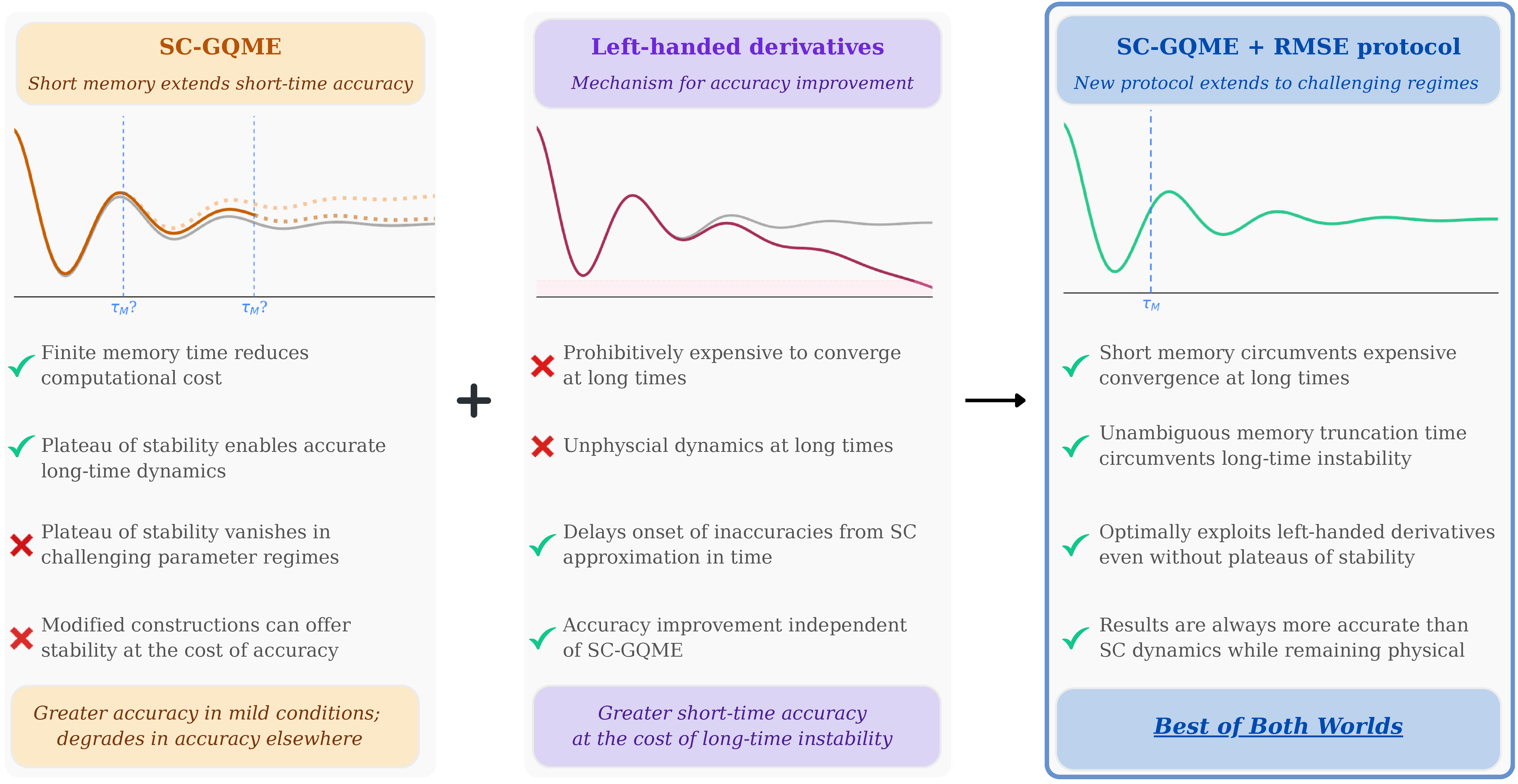
The SC-GQME does provide a tangible benefit over integrating left-handed time derivatives, and our analysis reveals when it is most advantageous. Specifically, when the memory kernel decays faster or even on similar timescales with the onset of inaccuracy—or even instability—in the left-handed derivatives, one can benefit from the latter’s enhanced short-time accuracy and generate accurate GQME dynamics for arbitrarily long times, even in parameter regimes where previous studies had encountered difficulties. We achieved this by reframing how to choose the memory cutoff, \(\tau_M\): instead of seeking a plateau of stability, which can become ambiguous in difficult parameter regimes, we shift to an RMSE-based analysis referenced to accessible SC dynamics to obtain a practical protocol for identifying a \(\tau_M\). This protocol addresses Q3: it is physically meaningful and yields predictions that are more accurate than the bare SC dynamics in parameter regimes where the traditional plateau does not exist. This approach further demonstrates that higher-order left-handed derivatives enhance short-time accuracy at the expense of long-time stability. This balance of short-time accuracy and long-time stability motivates the comparison of single- and mixed-accuracy kernel constructions that balance the competing effects, effectively extending the window of reliable short-time dynamics. Importantly, the protocol is pathway-agnostic by design and can in principle be applied to any combination of memory kernel constructions that differ in their level of short-time accuracy (see SI Sec. VI C). These ideas demonstrate that the SC-GQME is more than the sum of its constituent SC approximations: when paired with a principled cutoff strategy, it offers a robust framework for leveraging the short-time accuracy of SC dynamics to make reliable and physically meaningful predictions of long-time dynamics.
6 Conclusion and Outlook↩︎
In this work, we have addressed a fundamental and long-standing challenge in SC-GQMEs—how and when the SC-GQME improves the accuracy of semiclassical dynamics—through an extensive and systematic study. To resolve this main challenge, we addressed three main questions, Q1 – Q3, delineated in our introduction. We began by discovering that analytically acting with a (left-handed) time derivative on the initial condition of a SC correlation can improve its accuracy, even in the absence of the GQME. This finding allowed us to answer the first question (Q1) by demonstrating that the improvement could be understood through the short-time expansions of the exact and LSC-approximated correlation functions. However, we also showed that while left-handed derivatives can progressively improve short-time accuracy, they can become more inaccurate, and even unphysical, at long times, especially in parameter regimes that are challenging to SC theory. What is more, their integrated dynamics did not exactly match the predictions from the SC-GQME, especially at long times. This latter discrepancy between integrated and SC-GQME dynamics prompted us to address the second question (Q2) and show how the self-consistent SC-GQME formulation can (i) appear to preserve physical constraints, such as conservation of population, and (ii) alter the predicted dynamics by mixing time derivatives with various levels of accuracy. Having resolved these apparent discrepancies, we turned to the third question (Q3) by leveraging these novel insights with the finite lifetime of the SC-GQME’s memory kernel to reap the benefits of short-time accuracy from these derivatives while avoiding the dangers of their long-time instability. We achieved this by introducing a new protocol that employs an RMSE metric evaluated with respect to the LSC dynamics to unambiguously identify a beneficial kernel cutoff. Our protocol avoids the difficulties of previous approaches relying on a plateau of stability, which is known to disappear in difficult parameter regimes. Instead, we leverage the self-consistent structure of the memory kernel to construct single-accuracy and mixed-accuracy kernels to triangulate the latest point at which the resulting memory kernels exhibit short-time accuracy. We proposed this point as a proxy for the kernel cutoff time, and demonstrated that it gives truncated dynamics with greater accuracy than the bare LSC approximation and of the integrated left-handed derivatives even in parameter regimes where previous protocols have failed. For a schematic summary of the key findings in our work, we refer the reader to Fig. 9.
These insights open the door to applying the SC-GQME as a principled and reliable tool, and generalizing it to problems beyond model systems, even when one does not have access to exact benchmarks. By providing a clear framework for balancing the short-time accuracy of left-handed derivatives with the long-time stability enabled by memory truncation, our work enables the SC-GQME to deliver dynamics that are more accurate than the direct SC approximation. This approach is directly applicable to a wide variety of problems, including charge and energy transport and linear and non-linear spectroscopies where both transient and long-time accuracy is imperative. More broadly, our findings suggest that the SC-GQME can be systematically leveraged to capture the quantum dynamics of increasingly complex and atomistic environments, even ones with non-Gaussian statistics.
Supplemental Material↩︎
See the supplementary material for additional details supporting this work, including the generality of the conclusions, computational details, derivations of short-time analysis and population conservation, and additional details on the RMSE protocol.
Acknowledgments↩︎
This work was supported by the National Science Foundation Early Career Award in the directorate for Mathematical and Physical Sciences under Award No. 2443961. A.M.C. acknowledges the support from a David and Lucile Packard Fellowship for Science and Engineering. This work utilized the Alpine high-performance computing resource at the University of Colorado Boulder. Alpine is jointly funded by the University of Colorado Boulder, the University of Colorado Anschutz, Colorado State University, and the National Science Foundation (award 2201538). We thank Tianchu Li for sharing his HEOM code with us. We thank Aaron Kelly for sharing his FBTS code with us. M. R. L. thanks Ethan H. Fink for insightful discussions. We collectively thank Anthony J. Dominic III, Zachary R. Wiethorn, and Pranay Venkatesh for comments on the manuscript.
Author Declarations↩︎
Conflict of Interest↩︎
The authors have no conflicts to disclose.
Data Availability↩︎
The data that support the findings of this study are available from the corresponding author upon reasonable request.