Autonomous Satellite Rendezvous via Hybrid Feedback Optimization
February 24, 2026
Abstract
As satellites have proliferated, interest has increased in autonomous rendezvous, proximity operations, and docking (ARPOD). A fundamental challenge in these tasks is the uncertainties when operating in space, e.g., in measurements of satellites’ states, which can make future states difficult to predict. Another challenge is that satellites’ onboard processors are typically much slower than their terrestrial counterparts. Therefore, to address these challenges we propose to solve an ARPOD problem with feedback optimization, which computes inputs to a system by measuring its outputs, feeding them into an optimization algorithm in the loop, and computing some number of iterations towards an optimal input. We focus on satellite rendezvous, and satellites’ dynamics are modeled using the continuous-time Clohessy-Wiltshire equations, which are marginally stable. We develop an asymptotically stabilizing controller for them, and we use discrete-time gradient descent in the loop to compute inputs to them. Then, we analyze the hybrid feedback optimization system formed by the stabilized Clohessy-Wiltshire equations with gradient descent in the loop. We show that this model is well-posed and that maximal solutions are both complete and non-Zeno. Then, we show that solutions converge exponentially fast to a ball around a rendezvous point, and we bound the radius of that ball in terms of system parameters. Simulations show that this approach provides up to a 98.4% reduction in the magnitude of disturbances across a range of simulations, which illustrates the viability of hybrid feedback optimization for autonomous satellite rendezvous.
1 Introduction↩︎
Autonomous rendezvous, proximity operations, and docking (ARPOD) is a critical class of tasks for satellites in space [1]–[3]. The execution of ARPOD tasks allows for transportation of personnel, resupply, and servicing/repair [4]–[6]. However, due to satellite payload restrictions and financial costs, computing power onboard satellites is limited [7]–[9], which restricts the speed of computations that are performed when executing such tasks. Additionally, unanticipated modeling errors can cause poor performance and, potentially, cause mission failure, in part because predictions of future satellite states are unreliable [10], [11]. What we seek is an ARPOD approach that (i) does not predict future states, (ii) rejects disturbances when they arise, and (iii) has low computational complexity that accommodates the slow processors often found onboard satellites.
Therefore, in this paper we solve an ARPOD problem with feedback optimization. Feedback optimization measures the outputs of a control system, feeds them into a running optimization algorithm in the loop, and uses that algorithm to compute new inputs to a system [12]. Feedback optimization avoids solving optimization problems offline in a feedforward configuration [13]–[19]. It offers inherent robustness to inaccurate system models and time-varying parameters, and eliminates the need for pre-computed set points or reference signals [13], [15]. It differs fundamentally from model-predictive control (MPC) because it does not attempt to predict future states [20]. Such predictions can be difficult under the uncertainties that arise in space-based autonomy, which makes feedback optimization a natural fit. In general, feedback optimization also does not require an optimal input to be computed exactly by the optimization algorithm in the loop. Instead, some number of steps can be taken to compute iterates that work toward the optimal input, and one of those iterates can be used as a sub-optimal input to a system. This property helps accommodate slow processors onboard satellites, which may not be able to exactly compute optimal inputs before an input to a satellite is needed.
We focus on a satellite rendezvous problem in which there are two satellites, the target and the chaser, that are in low earth orbit. The target satellite is uncontrolled and orbiting the earth, while the chaser satellite is controlled. The goal is to drive the chaser to rendezvous with the target. Under mild conditions, we can linearize the chaser’s dynamics to obtain the Clohessy-Wiltshire (CW) equations [21], which describe the motion of the chaser relative to the target. It is standard in feedback optimization to assume that a system is asymptotically stable before optimizing its inputs [22]. However, the CW equations give a marginally stable system. Therefore, we first design a stabilizing feedback controller for the CW equations, and we show that only a subset of available gains must be non-zero to set all closed-loop eigenvalues to desired values. We also derive closed forms for each gain in terms of the desired closed-loop eigenvalues.
The stabilized CW equations that model the chaser are in continuous time, and we implement feedback optimization with discrete-time gradient descent running in the chaser’s feedback loop. We therefore model this setup as a hybrid system. We develop this model in the hybrid systems framework of [23], and we establish the existence and certain properties of its solutions, which we use to characterize the long-term performance of feedback optimization for the satellite rendezvous problem. To the best of our knowledge, this work is the first to apply feedback optimization to an ARPOD problem. In detail, the contributions of this paper are the following:
We design a controller to asymptotically stabilize the CW equations, and we give closed forms for the gains needed to attain desired closed-loop eigenvalues (Theorem 1).
We develop a hybrid systems model of feedback optimization for the CW equations with gradient descent in the loop, we prove that it is well-posed, and we prove that all maximal solutions to it are both complete and non-Zeno (Lemma 1, Proposition 1).
We bound the steady-state rendezvous error of the chaser satellite in terms of disturbances and other system parameters (Proposition 2, Theorem 2).
We prove that this implementation of feedback optimization is robust to perturbations, in the sense that bounded perturbations to the hybrid model produce bounded perturbations in the chaser’s trajectories (Corollary 1).
We show in simulations that hybrid feedback optimization successfully reduces the magnitude of disturbances in satellite rendezvous by up to 98.4% (Section 7).
A number of related approaches have been developed to solve ARPOD problems. For example, the authors in [24], [25] propose a switching controller that assures local asymptotic stability despite drift and under-actuation in the underlying satellite dynamics. Researchers have also used nonlinear estimators and sliding mode control to execute ARPOD maneuvers in the presence of faulty thrusters and physical disturbances in space [26]. To meet real-time demands, developments in [5], [27] provide a model-predictive control (MPC) approach that is computationally time-constrained and robust to disturbances drawn from a Gaussian distribution. We differ from all of these works by considering a hybrid model in which a continuous-time chaser satellite is controlled by a discrete-time optimization algorithm it runs onboard. The feedback optimization controller that we present also has lower computational complexity than the aforementioned works because it only requires some number of gradient descent iterations to be performed when computing each of the chaser’s inputs. To the best of our knowledge, this work is the first to apply feedback optimization to an ARPOD problem.
Within the feedback optimization literature, related work in [22], [28], [29] considers a continuous-time system and discrete-time computations in a sampled-data feedback optimization configuration. Results in [22], [28] show that large enough sample times guarantee closed-loop stability, and they provide practical stability guarantees under time-varying disturbances. Results in [29] show that when a closed-loop system’s inputs change at a fixed rate, global exponential stability is obtained. The current paper differs because we develop a hybrid model in the framework of [23], which allows us to characterize system behavior at all times, rather than just at certain sample times. Moreover, we use the hybrid model to derive analytical guarantees of robustness, including robustness to errors in the rate at which inputs are applied to the chaser, which we allow to vary over time. Some of our modeling developments are related to those in [30] by a subset of the authors of the current paper, which also considered hybrid feedback optimization. However, the current paper differs because it must analyze state dynamics that are subject to unknown, time-varying disturbances (see Section 4), while developments in [30] studied an unperturbed state equation.
The rest of the paper is organized as follows. Section 2 provides background, and Section 3 gives a formal problem statement. Section 4 develops a stabilizing controller, and Section 5 develops the hybrid feedback optimization model of the chaser satellite. Section 6 analyzes the convergence of the chaser to a rendezvous point. Section 7 presents simulations, and Section 8 concludes.
2 Preliminaries and Background↩︎
This section gives background on the Clohessy-Wiltshire equations, feedback optimization, and hybrid systems.
2.1 Notation↩︎
Let \(\mathbb{R}\) denote the set of real numbers and \(\mathbb{N}\) denote the set of non-negative integers. Let \(I_n\) denote the \(n \times n\) identity matrix and let \(\mathbb{1}_{n}\) denote the all-ones vector of size \(n\). Given scalars \(a_1, a_2, \ldots, a_n\), we use \(\textrm{diag}(a_1, a_2, \ldots, a_n)\) to denote the diagonal matrix with \(a_1, a_2, \ldots, a_n\) on its main diagonal. The \(2\)-norm of a vector \(\mathbf{x}\) is denoted \(\left\|\mathbf{x}\right\|\). We denote the Euclidean projection of a vector \(\mathbf{v}\) onto a non-empty, compact, convex set \(\mathcal{Z}\) by \(\Pi_{\mathcal{Z}}[\mathbf{v}] = \arg\min_{\mathbf{z} \in \mathcal{Z}} \|\mathbf{v}-\mathbf{z}\|\). The distance from a point \(\mathbf{v} \in \mathbb{R}^n\) to a non-empty set \(\mathcal{A} \subseteq \mathbb{R}^n\) is denoted \(\|\mathbf{v}\|_{\mathcal{A}} := \inf_{\mathbf{a} \in \mathcal{A}} \|\mathbf{v} - \mathbf{a}\|\). We denote the diameter of a non-empty, compact, convex set \(\mathcal{Z}\) by \(d_{\mathcal{Z}}\). Let \(\textrm{eig}(M)\) denote the set of eigenvalues of a square matrix \(M\). Let \(\lambda_{max}(M)\) denote the largest eigenvalue of a symmetric matrix \(M\), and let \(\lambda_{min}(M)\) denote its smallest eigenvalue. For a finite multi-set \(S\), we use \(\mu_{\max}(S)\) to denote the largest multiplicity of an element of \(S\), i.e., the largest number of times an element appears in \(S\).
2.2 Clohessy-Wiltshire Equations↩︎
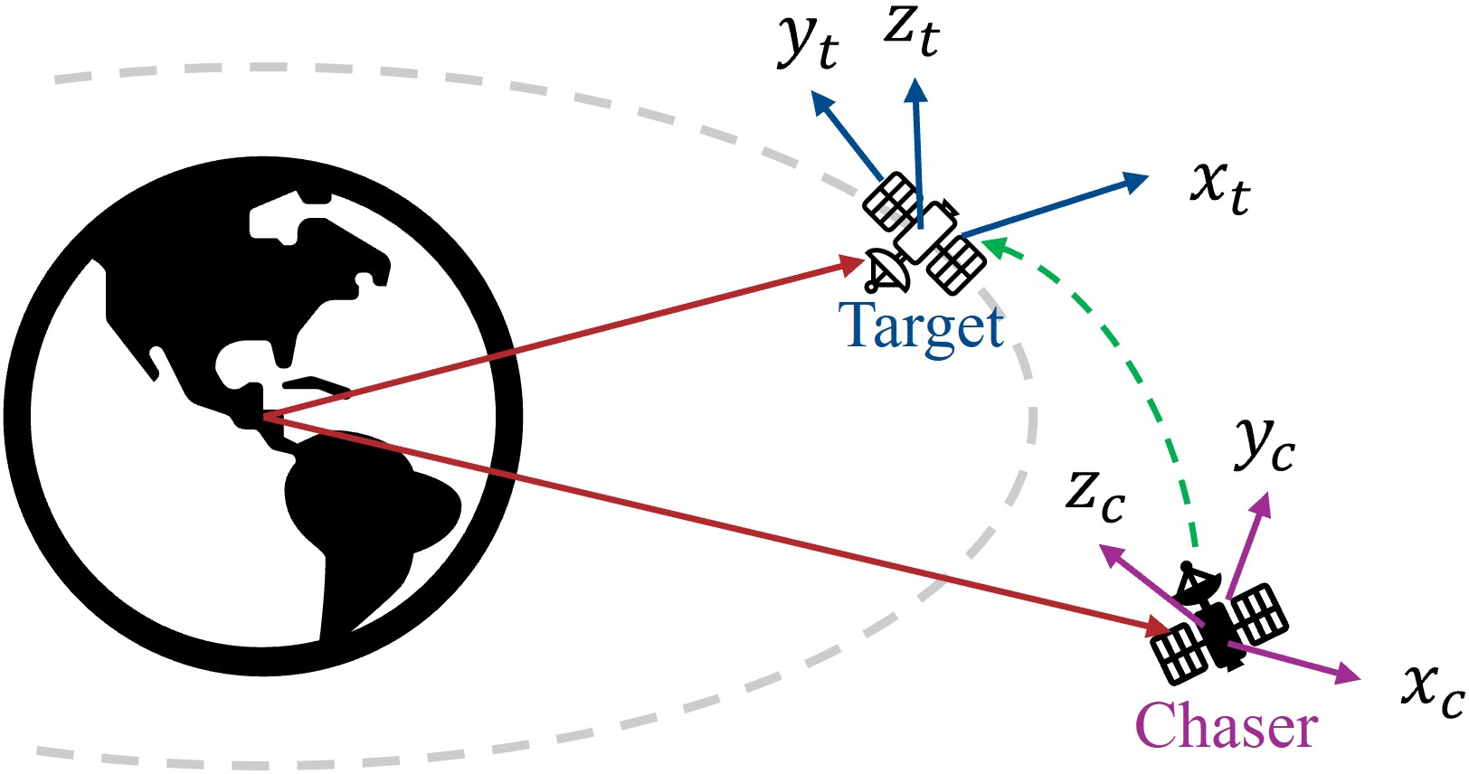
As described in the Introduction, we study the satellite rendezvous problem seen in Figure 1. We consider the relative dynamics between a controlled chaser satellite and an uncontrolled target satellite. To model these dynamics, we make the following standard assumptions [3], [5]:
The target satellite is in an uncontrolled circular orbit around the earth.
The distance between the target and chaser satellites is much less than the orbital radius of the target satellite.
The chaser satellite operates with bi-directional thrusters and external torque generators installed along the axes aligning with its body-fixed coordinate frame.
Then one can obtain the dynamics for the chaser’s position and velocity relative to the target. We denote the chaser’s position relative to the target by \((x, y, z)^T \in \mathbb{R}^3\), and linearizing these dynamics gives the Clohessy–Wiltshire (CW) equations: \[\label{eq:cwDynamics} \left[ \begin{array}{c} \dot{x} \\ \dot{y} \\ \dot{z} \\ \ddot{x} \\ \ddot{y} \\ \ddot{z} \end{array} \right] = \left[ \begin{array}{cccccc} 0 & 0 & 0 & 1 & 0 & 0 \\ 0 & 0 & 0 & 0 & 1 & 0 \\ 0 & 0 & 0 & 0 & 0 & 1 \\ 3w^2 & 0 & 0 & 0 & 2w & 0 \\ 0 & 0 & 0 & -2w & 0 & 0 \\ 0 & 0 & -w^2 & 0 & 0 & 0 \end{array} \right] \left[ \begin{array}{c} {x} \\ {y} \\ {z} \\ \dot{x} \\ \dot{y} \\ \dot{z} \end{array} \right] + \frac{1}{m_c} \left[ \begin{array}{ccc} 0 & 0 & 0 \\ 0 & 0 & 0 \\ 0 & 0 & 0 \\ 1 & 0 & 0 \\ 0 & 1 & 0 \\ 0 & 0 & 1 \end{array} \right] \left[ \begin{array}{c} {u_{x}} \\ {u_{y}} \\ {u_{z}} \end{array} \right],\tag{1}\] where \(m_c\) is the mass of the chaser, \(w := \sqrt{\mu/a^3}\), \(\mu := 3.986 \times10^{14} m^3s^{-2}\) is the standard gravity parameter of the earth, and \(a\) is the orbital radius of the satellite. These equations model the translational motion of the chaser relative to the target in the CW coordinate frame that is fixed to the target satellite. The CW equations define a marginally stable system, and we compactly express these dynamics as \[\label{eq:cwdynamics} \textcolor{black}{\dot{\boldsymbol{x}}} = A_{\textrm{CW}}\textcolor{black}{\boldsymbol{x}} + B_{\textrm{CW}}\mathbf{u},\tag{2}\] where \(\textcolor{black}{\boldsymbol{x}} = (x, y, z, \dot{x}, \dot{y}, \dot{z})^T \in \mathbb{R}^6\) and the matrices \(A_{\textrm{CW}} \in \mathbb{R}^{6 \times 6}\) and \(B_{\textrm{CW}} \in \mathbb{R}^{6 \times 3}\) can be read off from 1 .
2.3 Feedback Optimization Background↩︎
Suppose we have the linear time invariant (LTI) system \[\begin{align} \label{eq:ltisystem} \begin{aligned} \textcolor{black}{\dot{\mathbf{\chi}}} &= A\textcolor{black}{\mathbf{\chi}} + B\mathbf{v} \\ \mathbf{y} &= \Psi\mathbf{x} + \mathbf{d}, \end{aligned} \end{align}\tag{3}\] where \(\textcolor{black}{\mathbf{\chi}} \in \mathbb{R}^n\) is the system’s state, \(\mathbf{v} \in \mathbb{R}^m\) is its input, and \(\mathbf{y} \in \mathbb{R}^p\) is its output. The mapping \(t \mapsto \mathbf{d}(t) \in \mathbb{R}^p\) models an unknown time-varying disturbance.
In feedback optimization, it is standard to take \(A\) to be Hurwitz and we suppose that is the case here. If the mapping \(t \mapsto \mathbf{d}(t)\) were known, then to optimize the system’s steady-state behavior, at each \(t\) one could drive the pair \((\mathbf{v}, \mathbf{y})\) to a solution of
|l| ^ss,^ss (^ss,^ss)
where \(\Phi : \mathbb{R}^m \times \mathbb{R}^p \to \mathbb{R}\) is strongly convex in \((\mathbf{v}^{ss}, \mathbf{y}^{ss})\) and \(\mathcal{U} \subseteq \mathbb{R}^m\) is a non-empty, compact, convex set. These properties ensure the problem in [eq:phidef]-[eq:ddef] has a unique solution.
For Hurwitz \(A\), if \(\mathbf{d} \equiv 0\), then the steady-state input-to-output map of the system in 3 would be \(\mathbf{v}^{ss} \mapsto H\mathbf{v}^{ss}\), where \(H:= -\Psi A^{-1}B\). We allow for \(\mathbf{d} \neq 0\), and therefore we consider the mapping \(\mathbf{v}^{ss} \mapsto H\mathbf{v}^{ss} + \mathbf{d}\), which is equal to the steady-state mapping with its value perturbed by \(\mathbf{d}\). If the disturbance \(\mathbf{d}\) were known, then one could plug the expression for \(\mathbf{y}^{ss}\) in [eq:ddef] into [eq:phidef] and solve the set-constrained problem
|l| ^ss (^ss,H^ss + ) .
Then, one could, for example, solve this problem using a standard projected gradient descent law in which each gradient descent step is projected onto the constraint set \(\mathcal{U}\) to enforce the satisfaction of the set constraint. We denote the \(k^{\textrm{th}}\) iterate of this projected gradient descent law by \(\mathbf{v}^{ss}_k\). Then, the first iterate would take the form \[\label{eq:newbiggrad} \mathbf{v}^{ss}_{1} = \Pi_{\mathcal{U}}\Big[\mathbf{v}^{ss}_{0} -\gamma\Big(\nabla_{\mathbf{u}} \Phi\big(\mathbf{v}^{ss}_0, H\mathbf{v}^{ss}_0 + \mathbf{d}\big) + H^T \nabla_{\mathbf{y}}\Phi\big(\mathbf{v}^{ss}_0, H\mathbf{v}^{ss}_0 + \mathbf{d}\big)\Big)\Big],\tag{4}\] where \(\gamma > 0\) is a stepsize, \(\nabla_{\mathbf{u}} \Phi\) denotes the gradient of \(\Phi\) with respect to its first argument, and \(\nabla_{\mathbf{y}} \Phi\) denotes the gradient of \(\Phi\) with respect to its second argument.
However, we consider unknown disturbances \(t \mapsto \mathbf{d}(t)\), which means that the value of \(\mathbf{y}^{ss}\) cannot be computed from \(\mathbf{v}^{ss}\) with [eq:ddef]. Then, the update law in 4 also cannot be executed as written. Instead, rather than computing \(\mathbf{y}^{ss}\), we will sample the actual values of the output \(\mathbf{y}\) and use those values to optimize over \(\mathbf{v}^{ss}\). Let \(\mathbf{y}_s\) denote a sampled value of the output. Although \(\mathbf{y}_s\) need not be sampled from a system at steady state, we will use the standard approximation in feedback optimization that treats \(\mathbf{y}_s\) as coming from a system at steady state [13], [31]. This approximation is implemented by setting \(\mathbf{y}_s = H\mathbf{v}^{ss}_0 + \mathbf{d}\), where \(\mathbf{d}\) is the disturbance at the time \(\mathbf{y}_s\) is sampled and \(\mathbf{v}_0^{ss}\) is the input at the time \(\mathbf{y}_s\) is sampled.
Then, we can solve the problem in [eq:fo95genform] with a projected gradient descent law whose \((k+1)^{\textrm{th}}\) iterate takes the form \[\label{eq:gdUpdateLaw} \mathbf{v}^{ss}_{k+1} = \Pi_{\mathcal{U}}\Big[\mathbf{v}^{ss}_{k} -\gamma\Big(\nabla_{\mathbf{u}} \Phi\big(\mathbf{v}^{ss}_k, \mathbf{y}_s\big) + H^T \nabla_{\mathbf{y}}\Phi\big(\mathbf{v}^{ss}_k, \mathbf{y}_s\big)\Big)\Big].\tag{5}\]
In the feedback optimization literature, it is standard to formulate a closed-loop system between the plant in 3 and the optimization algorithm in 5 . Then the closed-loop interconnected system is \[\begin{align} \label{eq:cdltisystem} \text{Plant: }& \begin{cases} \textcolor{black}{\dot{\mathbf{\chi}}} &= A\textcolor{black}{\mathbf{\chi}} + B\mathbf{v} \\ \mathbf{y} &= \Psi\textcolor{black}{\mathbf{\chi}} + \mathbf{d}, \end{cases}\\ \text{Controller:}& \begin{cases} \mathbf{v}^{ss}_{k+1} = \Pi_{\mathcal{U}}\Big[\mathbf{v}^{ss}_{k} -\gamma\Big(\nabla_{\mathbf{u}} \Phi\big(\mathbf{v}^{ss}_k, \mathbf{y}_s\big) + H^T \nabla_{\mathbf{y}}\Phi\big(\mathbf{v}^{ss}_k, \mathbf{y}_s\big)\Big)\Big], \end{cases} \end{align}\tag{6}\] where at certain points in time we set \(\mathbf{y}_s = \mathbf{y}\) and \(\mathbf{v} = \mathbf{v}^{ss}_k\). Feedback optimization does not require the gradient descent update law to converge to an optimum before using one of its iterates as the input to the plant. Our analysis below allows for this possibility onboard the chaser satellite as well.
2.4 Hybrid System Background↩︎
Using the framework of [23] a hybrid system \(\mathcal{H}\) takes the form \[\label{eq:hybridmodel} \mathcal{H} := \begin{cases} \begin{align} \dot{\zeta} &\in F(\zeta) \quad &\zeta \in C \\ \zeta^+ &\in G(\zeta) \quad &\zeta \in D \end{align} \end{cases},\tag{7}\] where \(\zeta \in \mathbb{R}^{n}\) is the system’s state vector and the maps \(F\) and \(G\) are set-valued in general. The map \(F\) defines the flow map and governs the continuous dynamics within the flow set \(C\), while \(G\) defines the jump map, which models the system’s discrete behavior within the jump set \(D\).
Definition 1 (Hybrid Basic Conditions [23]). A hybrid system \(\mathcal{H}\) with data \((C, F, D, G)\) satisfies the hybrid basic conditions if
\(C\) and \(D\) are closed subsets of \(\mathbb{R}^n\);
\(F: \mathbb{R}^n\rightrightarrows\mathbb{R}^n\) is outer semicontinuous4, and locally bounded5 relative to \(C\), \(C\subset \text{dom}~F,\) and \(F(\zeta)\) is convex for every \(\zeta \in C\);
\(G: \mathbb{R}^n\rightrightarrows\mathbb{R}^n\) is outer semicontinuous and locally bounded relative to \(D\), and \(D\subset \text{dom}~G\).
If a hybrid system satisfies the hybrid basic conditions, then it is well-posed by [23], which implies that errors in the models of \(C\), \(D\), \(F\), and \(G\) up to a certain threshold produced bounded changes in the trajectories produced by the system over finite hybrid time horizons. For a hybrid system \(\mathcal{H}\), its solutions, denoted by \(\phi\), are hybrid arcs that can in general be maximal6, complete7, and Zeno8. Complete solutions are defined over arbitrarily long hybrid time horizons, and Zeno behavior implies that solutions undergo an infinite number of jumps in finite time, i.e., a system’s states stop flowing in finite time.
3 Problem Statement↩︎
As described in the Introduction, the goal of this work is to develop a computation-in-the-loop approach to autonomous satellite rendezvous that (i) does not require predictions of future states, (ii) allows for in-the-loop computations of inputs to be slow and hence to produce sub-optimal inputs, and (iii) provides robustness to unmodeled disturbances. In general, rendezvous of the chaser with the target at the exact same location would cause a collision and is therefore undesirable. Moreover, under the above conditions we do not expect exact convergence to a rendezvous point. Instead, we seek to show approximate convergence to a Euclidean ball about a desired rendezvous point. Accounting for all of these factors, the problem we solve in this paper is the following.
Problem 1. Develop a controller that drives the chaser satellite to asymptotically approximately rendezvous with the target satellite without attempting to predict future states, while using only onboard computations. Show that this controller is robust to perturbations in the chaser’s dynamics.
4 Stabilization of the Clohessy-Wiltshire Dynamics↩︎
We consider the CW equations from 2 with full-state feedback and unknown disturbances in output measurements. This setup is equivalent to 3 with \(A = A_{\textrm{CW}}\), \(B = B_{\textrm{CW}}\), and \(\Psi = I_6\). Then \[\begin{align} \dot{\mathbf{x}} &= A_{\textrm{CW}}\mathbf{x} + B_{\textrm{CW}}\mathbf{v} \\ \mathbf{y} &= \mathbf{x} + \mathbf{d}, \end{align}\] where \(\mathbf{d} \in \mathbb{R}^6\) is an unknown time-varying disturbance. We implement a controller of the form \(\mathbf{v}=-K\mathbf{y} + \mathbf{u}\), where \(\mathbf{u} \in \mathbb{R}^3\) is a new input that will be computed by the optimization algorithm in the loop, and \[K := \left[\begin{array}{cccccc} k_1 & k_2 & k_3 & k_4 & k_5 & k_6 \\ k_7 & k_8 & k_9 & k_{10} & k_{11} & k_{12} \\ k_{13} & k_{14} & k_{15} & k_{16} & k_{17} & k_{18} \end{array}\right] \in \mathbb{R}^{3 \times 6}\] is a matrix of gains. Then, the closed-loop system we consider takes the form \[\begin{align} \label{eq:CWltisystem} \dot{\mathbf{x}} &= A_{\textrm{stab}}\mathbf{x} + B_{\textrm{stab}}\mathbf{u} - B_{\textrm{stab}}K\mathbf{d} \\ \mathbf{y} &= \mathbf{x} + \mathbf{d}, \end{align}\tag{8}\] where \(B_{\textrm{stab}} := B_{\textrm{CW}}\) and \(A_{\textrm{stab}} := A_{\textrm{CW}} - B_{\textrm{CW}}K\). Explicitly, \[\label{eq:A95Stab} A_{\textrm{stab}} = \left[ \begin{array}{cccccc} 0 & 0 & 0 & 1 & 0 & 0 \\ 0 & 0 & 0 & 0 & 1 & 0 \\ 0 & 0 & 0 & 0 & 0 & 1 \\ 3w^2 - k_{1} & - k_{2} & - k_{3} & - k_{4} & 2w - k_{5} & - k_{6} \\ - k_{7} & - k_{8} & - k_{9} & -2w - k_{10} & - k_{11} & - k_{12} \\ - k_{13} & - k_{14} & -w^2 - k_{15} & - k_{16} & - k_{17} & - k_{18} \\ \end{array} \right].\tag{9}\] We suppose that a multi-set \(\Lambda_{\textrm{des}}\) of \(6\) desired closed-loop eigenvalues is given.
Assumption 1. All elements in \(\Lambda_{\textrm{des}}\) are real and negative.
We denote the elements of \(\Lambda_{\textrm{des}}\) by \(\lambda_1, \lambda_2, \ldots, \lambda_6\) and without loss of generality we suppose that \[\label{eq:lambda95order} \lambda_6 \leq \lambda_5 \leq \cdots \leq \lambda_1 < 0.\tag{10}\] Although the matrix \(K\) has \(18\) elements in it, we only set \(8\) of them to non-zero values, and they will be used in Theorem 1 to set all closed-loop eigenvalues equal to desired values. The non-zero gains we use are \(k_1\), \(k_4\), \(k_5\), \(k_8\), \(k_{10}\), \(k_{11}\), \(k_{15}\), and \(k_{18}\), and all other gains are set to zero. We set \(k_5 = 2w\) and \(k_{10} = -2w\).
Next we choose \(k_1\), \(k_4\), \(k_8\), \(k_{11}\), \(k_{15}\), and \(k_{18}\) so that \(\textrm{eig}\big(A_{\textrm{stab}}\big) = \Lambda_{\textrm{des}}\). We can do so because the CW equations are completely controllable. While standard pole placement techniques could be used to numerically assign gains in \(K\), we use fewer gains to provide a closed-form relationship between the gains and the desired closed-loop eigenvalues. We use this relationship in our later analysis to quantify how the choices of the closed-loop eigenvalues affect the chaser satellite’s rate of convergence to a compact ball about the rendezvous point with the target.
Theorem 1 (Stabilizing Controller Gains). Consider \(A_{\textrm{stab}}\) from 9 , let a multi-set of desired eigenvalues \(\Lambda_{\textrm{des}} = \{\lambda_1, \lambda_2, \ldots, \lambda_6\}\) be given, and suppose Assumption 1 holds. Then setting \[\label{eq:Kdef} K = \left[\begin{array}{cccccc} 3w^2 + \lambda_1\lambda_2 & 0 & 0 & -\lambda_1 - \lambda_2 & 2w & 0 \\ 0 & \lambda_3\lambda_4 & 0 & -2w & -\lambda_3 - \lambda_4 & 0 \\ 0 & 0 & -w^2 + \lambda_5\lambda_6 & 0 & 0 & -\lambda_5 - \lambda_6 \\ \end{array}\right]\tag{11}\] enforces \(\textrm{eig}(A_{\textrm{stab}}) = \Lambda_{\textrm{des}}\).
Proof. We first compute the eigenvalues of \(A_{\textrm{stab}}\) in terms of \(k_1\), \(k_4\), \(k_8\), \(k_{11}\), \(k_{15}\), and \(k_{18}\). The matrix \(\lambda I_6 - A_{\textrm{stab}}\) has a block \(2 \times 2\) structure, namely \[\lambda I_6 - A_{\textrm{stab}} = \left(\begin{array}{cc} \lambda I_3 & -I_3 \\ \textrm{diag}(k_1 - 3w^2, k_8, w^2 + k_{15}) & \textrm{diag}(\lambda + k_4, \lambda + k_{11}, \lambda + k_{18}) \end{array}\right).\] Using Schur’s formula [32], we have \[\begin{gather} \det(\lambda I_6 - A_{\textrm{stab}}) = \det(\lambda I_3)\det\Big(\textrm{diag}(\lambda + k_4, \lambda + k_{11}, \lambda + k_{18}) \\ + \textrm{diag}(k_1 - 3w^2, k_8, w^2 + k_{15})\big(\lambda I_3\big)^{-1}\Big). \end{gather}\] Expanding gives \[\begin{gather} \det(\lambda I_6 - A_{\textrm{stab}}) = \\ \det\Big(\textrm{diag}(\lambda^2 + k_4\lambda, \lambda^2 + k_{11}\lambda, \lambda^2 + k_{18}\lambda) + \textrm{diag}(k_1 - 3w^2, k_8, w^2 + k_{15})\Big), \end{gather}\] where we have used the fact that \(\det(cM) = c^3\det(M)\) for a scalar \(c\) and \(3 \times 3\) matrix \(M\). Then the eigenvalues of \(A_{\textrm{stab}}\) are the solutions to the equation \[\big(\lambda^2 + k_4\lambda + k_1 - 3w^2\big)\big(\lambda^2 + k_{11}\lambda + k_8\big)\big(\lambda^2 + k_{18}\lambda + k_{15} + w^2\big) = 0.\]
Solving this equation gives the eigenvalues of \(A_{\textrm{stab}}\) in pairs as the following: \(\lambda_{1,2} = -\frac{1}{2}k_4 \pm \frac{1}{2}\sqrt{k_4^2 - 4(k_1 - 3w^2)}\), \(\lambda_{3,4} = -\frac{1}{2}k_{11} \pm \frac{1}{2}\sqrt{k_{11}^2 - 4k_8}\), and \(\lambda_{5,6} = -\frac{1}{2}k_{18} \pm \frac{1}{2}\sqrt{k_{18}^2 - 4(w^2 + k_{15})}\). Starting with \(\lambda_{1}\) we see that \(\lambda_{1} = -\frac{1}{2}k_4 + \frac{1}{2}\sqrt{k_4^2 - 4(k_1 - 3w^2)}\), and solving for \(k_1\) gives \(k_{1} = 3w^2 - \lambda_{1}^2 - k_4\lambda_{1}\). We plug this expression into the expression for \(\lambda_{2}\) to find \(\lambda_{2} = -\frac{1}{2}k_4 - \frac{1}{2}\sqrt{k_4^2 - 4(k_1 - 3w^2)} = -\frac{1}{2}k_4 - \frac{1}{2}\big(2\lambda_1 + k_4\big)\). Then \(k_4 = -\lambda_{1} - \lambda_{2}\). Solving for \(k_8\), \(k_{11}\), \(k_{15}\), and \(k_{18}\) proceeds similarly. ◻
5 Hybrid Modeling of Feedback Optimization↩︎
In this section, we develop a hybrid model of feedback optimization for the satellite rendezvous problem, and we show that it is well-posed and that maximal solutions are both complete and non-Zeno. We first formulate the system model. As stated in Section 2.3, feedback optimization is used to optimize the steady-state behavior of a system, and systems are typically assumed to be asymptotically stable when using feedback optimization. We will therefore implement feedback optimization for the stabilized CW equations \[\tag{12} \begin{align} \dot{\mathbf{x}} &= A_{\textrm{stab}}\mathbf{x} + B_{\textrm{stab}}\mathbf{u} - B_{\textrm{stab}}K\mathbf{d} \tag{13} \\ \mathbf{y} &= \mathbf{x} + \mathbf{d}, \tag{14} \end{align}\] where we suppose that desired eigenvalues in \(\Lambda_{des}\) have been specified, \(K\) is from 11 , and \(\mathbf{d}\) is an unknown time-varying disturbance. At each time \(t\), we seek to drive the input and output of this system to the solution to
|l| , (,)
where \(H_{\textrm{stab}} := -A_{\textrm{stab}}^{-1}B_{\textrm{stab}}\), and the constraint \(\mathbf{y} = H_{\textrm{stab}}\mathbf{u} + \mathbf{d}\) is equal to the steady-state input-to-output mapping associated with the system in 13 14 with values perturbed by \(\mathbf{d}\). We consider objective functions \(\Phi\) of the form \[\label{eq:quadOBJ} \Phi(\mathbf{u},\mathbf{y}_{s}) = \frac{1}{2}\mathbf{u}^\top Q_{\mathbf{u}}\mathbf{u} + \frac{1}{2}(\mathbf{y}_{s} - \hat{\mathbf{y}})^\top Q_{\mathbf{y}}(\mathbf{y}_s - \hat{\mathbf{y}}),\tag{15}\] where \(Q_{\mathbf{u}} \in \mathbb{R}^{3 \times 3}\) and \(Q_{\mathbf{y}} \in \mathbb{R}^{6 \times 6}\) are symmetric and positive definite, and \(\hat{\mathbf{y}} \in \mathbb{R}^{6}\) is the nominal point at which the chaser will rendezvous with the target. The chaser should stop moving once it has done so, and therefore we set \(\hat{y}_4 = \hat{y}_5 = \hat{y}_6 = 0\).
5.1 Hybrid Modeling of Flow and Jump Sets↩︎
We now develop a hybrid model of feedback optimization implemented for the chaser’s dynamics in 12 with discrete-time gradient descent in the loop. Some of these modeling developments are related to those in prior work [30] by a subset of the authors of the current paper. The current paper goes beyond [30] because it implements a pre-stabilizing feedback controller design, propagates output disturbances through the dynamics as a result of that feedback controller, and quantifies the impact of these disturbances on satellite rendezvous.
We begin by defining the state vector and flow and jump sets for the model of the chaser. For feedback optimization, the state \(\mathbf{x} \in \mathbb{R}^6\) evolves in continuous time according to 13 , and \(\mathbf{x}\) is a state in the hybrid model we develop. Samples of the output are taken over time, and each sample is fed into an optimization algorithm that computes new values of \(\mathbf{u} \in \mathbb{R}^3\). We use \(\mathbf{y}_s \in \mathbb{R}^6\) to denote the sampled output, and both \(\mathbf{y}_s\) and \(\mathbf{u}\) are states of the hybrid system as well. The value of \(\mathbf{y}_s\) is plugged into a projected gradient descent algorithm of the form of 5 that runs in the loop and computes iterates that progress toward the optimal input. We denote the current gradient descent iterate by \(\mathbf{z} \in \mathbb{R}^3\), which is also a state of the hybrid system. To track the amount of continuous time required to compute an iterate, we introduce a timer \(\tau_{g} \in \mathbb{R}\) that tracks the amount of time remaining until the next gradient descent iteration is completed. It counts down with unit rate, and an iteration of gradient descent has been completed when it reaches zero. Between the times at which samples \(\mathbf{y}_s\) are taken, the state \(\mathbf{x}\) continues flowing with the most recently applied input held constant. Therefore, we introduce a timer \(\tau_{c} \in \mathbb{R}\) that tracks the amount of time remaining until the input to the system \(\mathbf{u}\) is changed. This timer also counts down with unit rate, and the input \(\mathbf{u}\) is set equal to the most recent optimization iterate \(\mathbf{z}\) when \(\tau_{c}\) reaches zero. Additionally, to convert the time-dependent disturbance \(t \mapsto \mathbf{d}(t)\) into a state-dependent disturbance, we introduce a timer \(\tau_{d}\in \mathbb{R}\) that begins at zero and counts up with unit rate. Each timer is a state of the hybrid model we develop.
We assemble the states of the hybrid system into the vector \[\label{eq:zeta} \zeta := \left(\begin{array}{ccccccc}\! \mathbf{x}^{\top} & \mathbf{u}^{\top} & \mathbf{y}_s^{\top} & \mathbf{z}^{\top} & \tau_{c} & \tau_{g} & \tau_{d} \end{array}\!\right)^{\top} \in \mathcal{X} := \mathbb{R}^{21}.\tag{16}\] We define \(\tau_{c,\max}\) as the maximum amount of time that can elapse between two consecutive changes in the chaser’s input, and it defines the control cadence of the chaser satellite. We define \(\tau_{g,\textrm{comp}}\) as the amount of time required to complete one iteration of gradient descent. A jump occurs only when \(\tau_{g}\) or \(\tau_{c}\) has reached zero. Otherwise the system’s states continue flowing. Then we define the flow and jump sets as \[\begin{align} C &:= \big\{\zeta \in \mathcal{X} \mid \tau_{c} \in [0,\tau_{c,\max}], \tau_{g} \in [0,\tau_{g,\textrm{comp}}]\big\} \tag{17} \\ D &:= \big\{\zeta \in \mathcal{X} \mid \tau_{c} = 0 \textrm{ or } \tau_{g} = 0\big\}, \tag{18} \end{align}\] respectively.
5.2 Flow Map Definition↩︎
The flow map models the continuous-time evolution of \(\zeta\). The state \(\mathbf{x}\) flows according to the stabilized CW dynamics in 13 , \(\tau_{g}\) and \(\tau_{c}\) count down with unit rate, and \(\tau_{d}\) counts up with unit rate. Other states only change at jump times, and the flow map is \[\label{eq:fwmap} F(\zeta) := \left(\begin{array}{c} A_{\textrm{stab}}\mathbf{x} + B_{\textrm{stab}}\mathbf{u} - B_{\textrm{stab}}K\mathbf{d}(\tau_{d}) \\ \mathbf{0} \\ \mathbf{0} \\ \mathbf{0} \\ {-1} \\ {-1} \\ {1} \end{array}\right) \quad \textcolor{black}{\textrm{ for all } \zeta \in C}.\tag{19}\]
5.3 Jump Map Definition↩︎
The jump map has three cases as defined in 18 : (i) \(\tau_{g} = 0\) with \(\tau_{c} > 0\), (ii) \(\tau_{c} = 0\) with \(\tau_{g} > 0\), and (iii) \(\tau_{c} = \tau_{g} = 0\).
In case (i), the hybrid system completes a single gradient descent step of the form \(\mathbf{z}^+ = \Pi_{\mathcal{U}}\big[\mathbf{z} - \gamma(\nabla_{\mathbf{u}} \Phi(\mathbf{z}, \mathbf{y}_s) + H^T\nabla_{\mathbf{y}}\Phi(\mathbf{z}, \mathbf{y}_s))\big]\), where \(\nabla_{\mathbf{u}}\Phi\) denotes the derivative of \(\Phi\) with respect to its first argument, \(\nabla_{\mathbf{y}}\Phi\) denotes the derivative of \(\Phi\) with respect to its second argument, and \(\gamma > 0\) is a stepsize. Since \(\tau_{c} > 0\), that new iterate is not applied as the input to the system. The timer \(\tau_{g}\) resets to \(\tau_{g,\textrm{comp}}\), and all other states remain unchanged. Then, the jump map for this case is \[\label{eq:g1def} G_1(\zeta) := \left(\begin{array}{c} \mathbf{x} \\ \mathbf{u} \\ \mathbf{y}_s \\ \Pi_{\mathcal{U}}\Big[\mathbf{z} - \gamma\big(\nabla_{\mathbf{u}} \Phi\big(\mathbf{z}, \mathbf{y}_s\big) + H^T\nabla_{\mathbf{y}}\Phi\big(\mathbf{z}, \mathbf{y}_s\big)\big)\Big] \\ \tau_{c} \\ \tau_{g,\textrm{comp}} \\ \tau_{d} \end{array} \right) \quad \textcolor{black}{\textrm{ for all } \zeta \in D_1},\tag{20}\] where \(D_1 := \{\zeta\in \mathcal{X}: \tau_{g} = 0\}\).
During case (ii), when \(\tau_{c} = 0\) and \(\tau_{g} > 0\), the input \(\mathbf{u}\) is set equal to the most recent optimization iterate \(\mathbf{z}\), a new output \(\mathbf{y}_s\) is sampled, and the timer \(\tau_{c}\) resets to some number in the interval \([\tau_{c,\min},\tau_{c,\max}]\), where \(0 < \tau_{c,\min} \leq \tau_{c,\max}\). This interval is used to model indeterminacy in the amount of time that elapses between changes in the input. All other states remain unchanged, and the jump map for this case is \[\label{eq:g2def} G_2(\zeta) := \left(\begin{array}{c} \mathbf{x} \\ \mathbf{z} \\ H_{\textrm{stab}}\mathbf{u} + \mathbf{d}(\tau_{d}) \\ \mathbf{z} \\ {[\tau_{c,\min}, \tau_{c,\max}]} \\ \tau_{g}\\ \tau_{d} \end{array} \right) \quad \textcolor{black}{\textrm{ for all } \zeta \in D_2},\tag{21}\] where \(D_2 := \{\zeta\in \mathcal{X}: \tau_{c} = 0\}\), and, as is standard in feedback optimization, we approximate the output \(\mathbf{y}_{s} = \Psi \mathbf{x} + \mathbf{d}\) as coming from the perturbed steady-state mapping \[\label{eq:hstab95approx} \mathbf{y}_{s} = H_{\textrm{stab}}\mathbf{u} + \mathbf{d},\tag{22}\] where \(H_{\textrm{stab}}\) is from [eq:ddef95u]. The mapping \(G_2\) has a set-valued element in the form of \([\tau_{c,\min}, \tau_{c,\max}]\), which allows \(\tau_{c}\) to reset to any value in this interval and models indeterminacy in the amount of time that elapses between changes in the input.
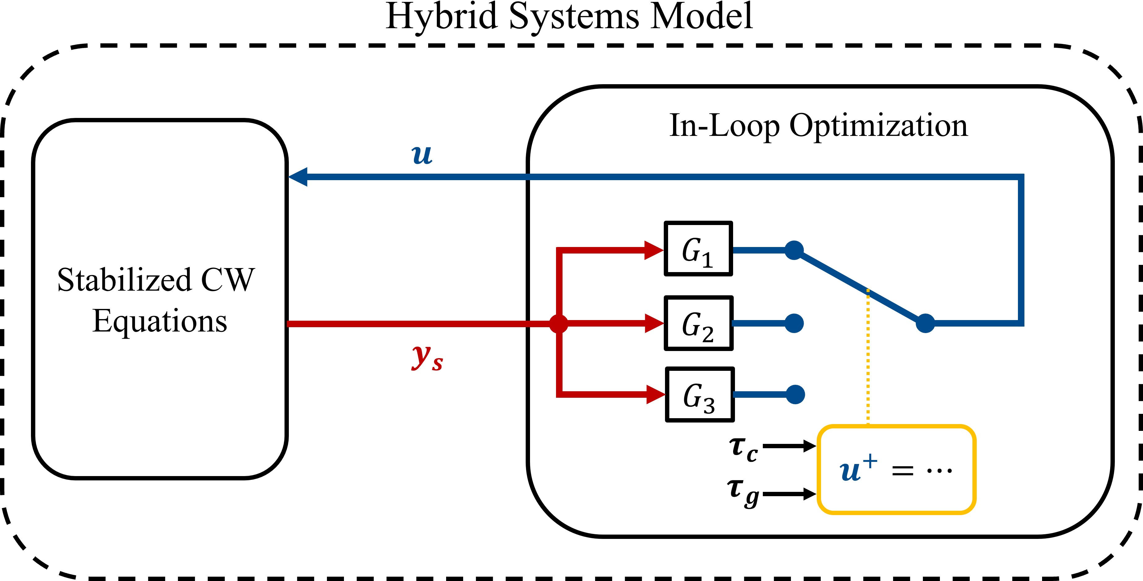
In case (iii), where both \(\tau_{c} = 0\) and \(\tau_{g} = 0\), we combine cases (i) and (ii), and the system executes either \(G_1\) then \(G_2\) or \(G_2\) then \(G_1\). The full jump map \(G\) is \[\label{eq:jpmap} \zeta^+ \in G(\zeta) := \begin{cases} G_1(\zeta) \quad \text{if } \tau_{c} > 0 \textrm{ and } \tau_{g} = 0 \quad \textrm{ Case (i)} \\ G_2(\zeta) \quad \text{if } \tau_{c} = 0 \textrm{ and } \tau_{g} > 0 \quad \textrm{ Case (ii)} \\ G_3(\zeta) \quad \text{if } \tau_{c} = 0 \textrm{ and } \tau_{g} = 0 \quad \textrm{ Case (iii)}, \end{cases}\tag{23}\] where \(G_3(\zeta) := G_1(\zeta) \cup G_2(\zeta)\). Then, the hybrid model of feedback optimization onboard the chaser satellite is \[\label{eq:hybridFO} \mathcal{H}_{\text{FO}}:= (C,F,D,G),\tag{24}\] where \(C\) is from 17 , \(F\) is from 19 , \(D\) is from 18 , and \(G\) is from 23 . We illustrate this hybrid model in Figure 2.
5.4 Intermittent Sampling and Optimization in \(\mathcal{H}_{\text{FO}}\)↩︎
We impose the following assumption on the relative rates of computation of inputs and changes in the values of inputs applied to the chaser.
Assumption 2. There exists \(\ell \in \mathbb{N}\) with \(\ell \geq 1\) such that \(\ell\tau_{g,\textrm{comp}} \leq \tau_{c,\min}\).
Assumption 2 implies that there are at least \(\ell\) gradient descent iterations, i.e., case (i) jumps, performed between consecutive changes in the chaser’s input. Mathematically, it ensures that the optimization algorithm takes at least one step towards the optimal input before each input is applied to the chaser. The value of \(\ell\) is determined by a chaser satellite’s onboard processor and will vary across implementations. Without this assumption, a satellite could never perform a computation and never change its input.
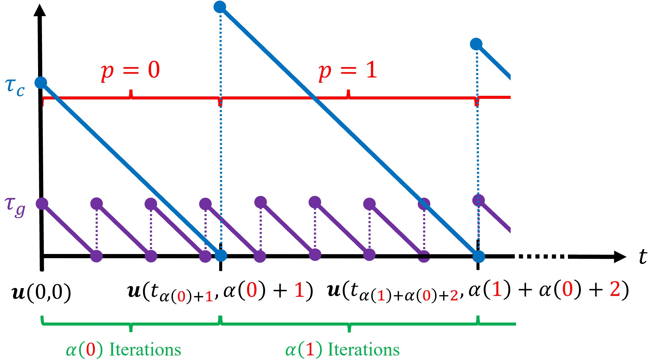
To analyze the relationship between sampling and optimization in \(\mathcal{H}_{\text{FO}}\), consider an initial condition \(\phi(0,0) = \nu \in \mathbb{R}^{21}\) that satisfies \[\label{eq:initconds} \tau_{c}(0,0) \in [\tau_{c,\min},\tau_{c,\max}],~\tau_{g}(0, 0) = \tau_{g,\textrm{comp}},~\tau_{d}(0,0) = 0,~\textrm{and}~\mathbf{z}_{0}({0},{0}) = \mathbf{u}({0},{0}),\tag{25}\] and consider a solution \(\phi\) to \(\mathcal{H}_{FO}\) from such initial condition. The behavior of sampling outputs and optimizing inputs is as follows. Starting from hybrid time \((0, 0)\) the input \(\mathbf{u}(0, 0)\) is applied to the system and held constant. While that input is applied, the system performs some number of gradient descent steps that we denote by \(\alpha(0)\) (which are \(\alpha(0)\) case (i) jumps) before a new input is applied. Each case (i) jump is triggered by \(\tau_{g}\) reaching zero. The new input is applied when a case (ii) jump occurs, which is triggered by \(\tau_{c}\) reaching zero. This case (ii) jump is the \(\big(\alpha(0) + 1\big)^{th}\) jump, and it changes the value of the input to \(\mathbf{u}({t_{\alpha(0) + 1}},{\alpha(0) + 1})\), where the value \(\alpha(0) + 1\) has accounted for the \(\alpha(0)\) case (i) jumps and the one case (ii) jump that have occurred. When computing the value of the input \(\mathbf{u}({t_{\alpha(0) + 1}},{\alpha(0) + 1})\), the \(k^{\textrm{th}}\) iterate for any \(k \in \{0, \ldots, \alpha(0)\}\) is denoted \(\mathbf{z}_{k}(t_{k},{k})\). When computing \(\mathbf{u}(t_{\alpha(0) + 1},{\alpha(0) + 1})\), we denote the \(\alpha(0)^{\textrm{th}}\) iterate (which is the last iterate) by \(\mathbf{z}_{\alpha(0)}(t_{\alpha(0)},{\alpha(0)})\). The first two changes in the input are shown in Figure 3, where \(\tau_{c}\) is shown jumping to different values when it jumps because it can jump to any value in the interval \([\tau_{c,\min}, \tau_{c,\max}]\).
When \(\tau_{c}\) reaches zero for the first time, several operations occur in addition to the input changing, and they are modeled in the jump map \(G_2\) in 21 . The output \(\mathbf{y}_s(t_{\alpha(0) + 1},{\alpha(0) + 1})\) is sampled, and we approximate it as coming from the perturbed steady-state mapping in 22 . The input \(\mathbf{u}\) is set equal to the most recent optimization iterate, i.e., \(\mathbf{u}(t_{\alpha(0) + 1},{\alpha(0) + 1}) = \mathbf{z}_{\alpha(0)}(t_{\alpha(0)},{\alpha(0)})\), and that iterate is also used as the initial iterate when computing the next input so that \(\mathbf{z}_{0}(t_{\alpha(0) + 1},{\alpha(0) + 1}) = \mathbf{z}_{\alpha(0)}(t_{\alpha(0)},{\alpha(0)})\).
We use \(\alpha(p)\) for \(p \in \mathbb{N}\) to denote the number of gradient descent iterations that are generated when computing the \((p+1)^{\textrm{th}}\) input to the system. We define \(\textcolor{black}{\bar{\alpha}\left(p\right)}\) for \(p \in \mathbb{N}\) as the total number of gradient descent iterations that have been completed for computing any input up until the \(p^{\textrm{th}}\) jump in \(\mathbf{u}\). Then \(\textcolor{black}{\bar{\alpha}\left(0\right)} = 0\) and \(\textcolor{black}{\bar{\alpha}\left(p\right)} = \sum^{p-1}_{i=0} \alpha(i)\). Figure 3 provides an illustration of how inputs change over time.
We can iterate the above analysis to find a general expression for the \((k+1)^{\textrm{th}}\) iterate when finding the \((p+1)^{\textrm{th}}\) input to the system. That iterate is computed after the \(p^{\textrm{th}}\) case (ii) jump has occurred and after \(k+1\) case (i) jumps have occurred after that case (ii) jump. It takes the form \[\begin{gather} \label{eq:bigiteration} \mathbf{z}_{k+1}(t_{\textcolor{black}{\bar{\alpha}\left(p\right)} + p + k + 1},{\textcolor{black}{\bar{\alpha}\left(p\right)} + p + k + 1}) = \\\Pi_{\mathcal{U}}\big[\mathbf{z}_{k}(t_{\textcolor{black}{\bar{\alpha}\left(p\right)} + p + k},{\textcolor{black}{\bar{\alpha}\left(p\right)} + p + k}) - \gamma\big(Q_{\mathbf{u}}\mathbf{z}_{k}(t_{\textcolor{black}{\bar{\alpha}\left(p\right)} + p + k},{\textcolor{black}{\bar{\alpha}\left(p\right)} + p + k}) \\ + H^{\top}Q_{\mathbf{y}}\big(\mathbf{y}_s(t_{\textcolor{black}{\bar{\alpha}\left(p\right)} + p + k},{\textcolor{black}{\bar{\alpha}\left(p\right)} + p + k}) - \hat{\mathbf{y}} \big)\big)\big]. \end{gather}\tag{26}\]
The hybrid time \((t_{\textcolor{black}{\bar{\alpha}\left(p\right)} + p + k},{\textcolor{black}{\bar{\alpha}\left(p\right)} + p + k})\) accounts for \(\bar{\alpha}(p)\) total gradient descent iterations that have been computed up to the \(p^{\textrm{th}}\) change in the input, \(p\) changes in the input itself, and \(k\) gradient descent iterations that have been computed so far in the course of computing the \((p+1)^{\textrm{th}}\) input.
The \((p+1)^{\textrm{th}}\) input to the system is \[\label{eq:c2inptiterate} \mathbf{u}(t_{\textcolor{black}{\bar{\alpha}\left(p + 1\right)} + p + 1},{\textcolor{black}{\bar{\alpha}\left(p + 1\right)} + p + 1}) = \mathbf{z}_{\alpha(p)}(t_{\textcolor{black}{\bar{\alpha}\left(p\right)} + \alpha(p) + p},{\textcolor{black}{\bar{\alpha}\left(p\right)} + \alpha(p) + p}),\tag{27}\] i.e., it is set equal to the most recently computed iterate from the optimization algorithm at the time that the change in the input occurs. When computing iterates for the \((p+2)^{\textrm{th}}\) input, the initial iterate is denoted \[\mathbf{z}_{0}(t_{\textcolor{black}{\bar{\alpha}\left(p + 1\right)} + p + 1},{\textcolor{black}{\bar{\alpha}\left(p + 1\right)} + p + 1}).\] That is, the initial iterate when computing the next input is equal to the final iterate that was computed when finding the previous input.
5.5 Basic Properties of the Hybrid Model of Feedback Optimization↩︎
We impose the following assumption on the disturbance \(\mathbf{d}\).
Assumption 3. There exists a non-empty compact set \(\mathcal{D} \subseteq \mathbb{R}^6\) such that \(\mathbf{d}(t) \in \mathcal{D}\) for all \(t \geq 0\). The mapping \(t \mapsto \mathbf{d}(t)\) is differentiable and there exists some \(\bar{\mathbf{d}} \geq 0\) such that \(\big\|\dot{\mathbf{d}}(t)\big\| \leq \bar{\mathbf{d}}\) for all \(t \geq 0\).
The following results show that solutions to \(\mathcal{H}_{\text{FO}}\) exist over arbitrarily long hybrid time domains.
Lemma 1. Consider the system \(\mathcal{H}_{\text{FO}}\) in 24 and suppose that Assumption 3 holds. Then \(\mathcal{H}_{\text{FO}}\) is well-posed in the sense that it satisfies Definition 1.
Proof. See 10.1 ◻
Lemma 1 guarantees well-posedness of the system, which is used in the forthcoming results. Next we establish that solutions to \(\mathcal{H}_{\text{FO}}\) exist for hybrid times \((t, j)\) where \(t\) and \(j\) can grow arbitrarily large.
Proposition 1 (Completeness of Maximal Solutions). Consider the hybrid feedback optimization model \(\mathcal{H}_{\text{FO}}\) from 24 and suppose Assumption 3 holds. Then, from every point in \(C\cup D\) there exists a nontrivial solution to \(\mathcal{H}_{\text{FO}}\), and all maximal solutions are both complete and non-Zeno.
Proof. See 10.2 ◻
The non-Zeno property guarantees that the system will keep flowing and that the computation and application of inputs will continue indefinitely.
6 Convergence Analysis↩︎
This section analyzes how the chaser approaches the target when using feedback optimization. For simplicity of notation we define \(\xi(p,k) := \bar{\alpha}(p) + p + k\). Then \[\label{eq:xtime95def} (t_{\xi(p,k)},{\xi(p,k)}) = (t_{\textcolor{black}{\bar{\alpha}\left(p\right)} + p + k},{\textcolor{black}{\bar{\alpha}\left(p\right)} + p + k}),\tag{28}\] i.e., \((t_{\xi(p,k)},{\xi(p,k)})\) denotes the hybrid time at which the optimization algorithm has completed the \(k^{\textrm{th}}\) iteration when computing the \((p+1)^{\textrm{th}}\) input to the system. Then we may write 26 as \[\begin{gather} \mathbf{z}_{k+1}(t_{\xi(p,k+1)},{\xi(p,k+1)}) = \Pi_{\mathcal{U}}\big[\mathbf{z}_{k}(t_{\xi(p,k)},{\xi(p,k)}) \\ - \gamma\big(Q_{\mathbf{u}}\mathbf{z}_{k}(t_{\xi(p,k)},{\xi(p,k)}) + H^\top Q_{\mathbf{y}}\big(\mathbf{y}_s(t_{\xi(p,k)},{\xi(p,k)}) - \hat{\mathbf{y}} \big)\big)\big]. \end{gather}\]
The following lemma relates successive iterates that are used to compute the inputs to the chaser satellite. In it, we use the constants \[\label{eq:LqDef} L := \lambda_{\max}(Q_{\mathbf{u}} + H_{\textrm{stab}}^{\top}Q_{\mathbf{y}}H_{\textrm{stab}}) \quad \textrm{and} \quad q:= 1-2\gamma\lambda_{\min}(Q_u) + \gamma^2L^2 \in (0,1),\tag{29}\] where \(Q_{\mathbf{u}}\) and \(Q_{\mathbf{y}}\) are from 15 and \(H_{\textrm{stab}}\) is from [eq:ddef95u].
Lemma 2 (Input Convergence Rate). Consider the hybrid system \(\mathcal{H}_{FO}\) in 24 and the objective in 15 . Suppose that the gradient descent algorithm uses a stepsize \(\gamma \in \left(0,\frac{2}{\lambda_{\min}(Q_u) + L}\right)\), where \(L\) is from 29 . Let \(\phi\) denote a maximal solution to \(\mathcal{H}_{FO}\) with initial condition \(\phi(0, 0) = \nu\) that satisfies 25 . For any \((t, j) \in \textrm{dom } \phi\), set \(P = \max\{p \in \mathbb{N} : \bar{\alpha}(p) + p \leq j\}\). Then, for any \(p \in \{0, \ldots, P\}\) the state \(z\) obeys \[\begin{gather} \label{eq:inputbound95norm} \big\|\mathbf{z}_{\alpha({p})}(t_{\xi(p,\alpha(p))},{\xi(p,\alpha(p))}) - \mathbf{z}^*(t_{\xi(p,0)},{\xi(p,0)})\big\| \\ \leq q^{\frac{\alpha({p})-1}{2}}\big\|\mathbf{z}_{1}(t_{\xi(p,1)},{\xi(p,1)}) - \mathbf{z}^*(t_{\xi(p,0)},{\xi(p,0)})\big\|, \end{gather}\tag{30}\] where \(q\) is from 29 and \(\mathbf{z}^*(t_{\xi(p,0)},{\xi(p,0)}) = \mathop{\mathrm{arg\,min}}\limits_{\mathbf{u} \in \mathcal{U}} \Phi\big(\mathbf{u}, \mathbf{y}_{s}(t_{\xi(p,0)},{\xi(p,0)})\) is a function of the hybrid time time \((t_{\xi(p,0)},{\xi(p,0)})\) because it depends on the sampled output at the same time, namely \(\mathbf{y}_{s}(t_{\xi(p,0)},{\xi(p,0)})\).
Proof. The steps of the proof follow those of a standard proof in the convex optimization literature for the minimization of a strongly convex function using gradient descent, e.g., [33]. ◻
6.1 Complete Hybrid Convergence↩︎
At time \(t\), let \(\big(\tilde{\mathbf{u}}(t), \tilde{\mathbf{y}}(t)\big)\) denote the solution to [eq:fo95genform95u]. Setting \(\dot{\mathbf{x}} \equiv 0\) in the CW equations and setting \(\mathbf{u}\) and \(\mathbf{y}\) equal to \(\tilde{\mathbf{u}}(t)\) and \(\tilde{\mathbf{y}}(t)\), respectively, we obtain the state \[\label{eq:xtildedef} \tilde{\mathbf{x}}(t) = -A_{\textrm{stab}}^{-1}B_{\textrm{stab}}\tilde{\mathbf{u}}(t) + A_{\textrm{stab}}^{-1}B_{\textrm{stab}}K\mathbf{d}(t),\tag{31}\] which simultaneously gives the CW equations the input \(\tilde{\mathbf{u}}(t)\), the output \(\tilde{\mathbf{y}}(t)\), and the input-output relation \(\tilde{\mathbf{y}}(t) = H_{\textrm{stab}}\tilde{\mathbf{u}}(t) + \mathbf{d}(t)\) as required by [eq:fo95genform95u]. The value of \(\tilde{\mathbf{x}}(t)\) in general differs from that of the nominal rendezvous point \(\hat{y}\) precisely because \(\tilde{\mathbf{x}}(t)\) accounts for costs on the input in \(\Phi\) and the disturbance \(\mathbf{d}\). The value of \(\tilde{\mathbf{x}}(t)\) can be interpreted as the chaser’s chosen rendezvous point at time \(t\). This section bounds the distance between \(\mathbf{x}(t, j)\) and \(\tilde{\mathbf{x}}(t)\) as a function of \(t\).
For a solution \(\phi\) to \(\mathcal{H}_{FO}\), at each hybrid time \((t, j) \in \textrm{dom }\phi\) we can bound the distance between \(\phi\) and the set \[\label{eq:closedsetA} \mathcal{A}(t) := \big\{\tilde{\mathbf{x}}(t)\big\} \times \mathcal{U} \times \mathbb{R}^6 \times \mathcal{U} \times [0, \tau_{c,\max}] \times [0, \tau_{g,\textrm{comp}}] \times \mathbb{R},\tag{32}\] where \(\tilde{\mathbf{x}}(t)\) is from 31 . By definition, \(\|\phi(t, j)\|_{\mathcal{A}(t)} = \|\mathbf{x}(t, j) - \tilde{\mathbf{x}}(t)\|\). We will bound \((t, j) \mapsto \|\phi(t, j)\|_{\mathcal{A}(t)}\) for each solution to \(\mathcal{H}_{\text{FO}}\), which will characterize the error between the chaser’s position \(\mathbf{x}(t,j)\) and the chosen rendezvous point \(\tilde{\mathbf{x}}(t)\), while accounting for the full dynamics of \(\mathcal{H}_{\text{FO}}\).
Proposition 2 (Convergence of \(\mathcal{H}_{\text{FO}}\)). Consider the hybrid system \(\mathcal{H}_{\text{FO}}\) from 24 , with the objective function from 15 and stepsize \(\gamma \in \left(0,\frac{2}{\lambda_{\min}(Q_u) + L}\right)\), where \(Q_{\mathbf{u}}\) is from 15 and \(L\) is from 29 . Suppose that Assumptions 1, 3, and 2 hold. For each maximal solution \(\phi\) to \(\mathcal{H}_{FO}\) with initial condition \(\phi(0, 0) = \nu\) that satisfies 25 , for each \((t, j) \in \textrm{dom } \phi\), we have \[\begin{gather} \label{eq:tmCompleteBound} \|\phi(t, j)\|_{\mathcal{A}(t)} \leq \mu_{\max}(\Lambda_{\textrm{des}})\frac{|\lambda_6|}{|\lambda_1|}\exp\big({-\big|\lambda_{1}\big|}t\big) \big\|\phi({0},{0})\big\|_{\mathcal{A}(t)}\\ + \frac{\mu_{\max}(\Lambda_{\textrm{des}})|\lambda_6|d_{\mathcal{U}}}{m_{c}\big|\lambda_{1}\big|^2}\big[2 - \exp(-|\lambda_1|\tau_{c,\max}) -\exp\big({-\big|\lambda_{1}\big|}t\big)\big] \\ + \frac{\mu_{\max}(\Lambda_{\textrm{des}})|\lambda_6| q^{\frac{\ell}{2}} d_{\mathcal{U}}}{m_{c}\big|\lambda_{1}\big|^2}\Big[1 - \exp\big({\big|\lambda_{1}\big|}\tau_{c,\min}\big)\exp\big({-\big|\lambda_{1}\big|}t\big)\Big] \\ + \frac{\mu_{\max}(\Lambda_{\textrm{des}}) |\lambda_6|}{m_{c}|\lambda_1|^2}\big\|A_{\textrm{stab}}^{-1}\big\|\big\|K\big\|\bar{\mathbf{d}} \Big[1 + \big(\mu_{\max}(\Lambda_{\textrm{des}})|\lambda_6|t - 1\big)\exp\big({-\big|\lambda_{1}\big|}t\big)\Big], \end{gather}\tag{33}\] where \(\bar{\mathbf{d}}\) is from Assumption 3, \(\ell \geq 1\) is from Assumption 2, \(\mathcal{A}(t)\) is from 32 , and \(q \in \left(0,1\right)\) is from 29 . In particular, each such solution satisfies \[\begin{gather} \limsup_{\substack{(t, j) \in \textrm{dom }\phi \\ t+j\rightarrow\infty}}\left\|\phi({t},{j})\right\|_{\mathcal{A}(t)} \leq \\ \mu_{\max}(\Lambda_{\textrm{des}})\frac{|\lambda_6|}{m_{c}|\lambda_1|^2} \Big(2d_{\mathcal{U}} -d_{\mathcal{U}}\exp({-\big|\lambda_{1}\big|}\tau_{c,\max}) + d_{\mathcal{U}}q^{\frac{\ell}{2}} + \big\|A_{\textrm{stab}}^{-1}\big\|\big\|K\big\|\bar{\mathbf{d}}\Big). \end{gather}\]
Proof. See 11.1. ◻
Proposition 2 shows that a chaser satellite approaches a ball around its chosen rendezvous point exponentially quickly with rate given by \(\exp(-|\lambda_1|t)\). At time \(t\) that chosen rendezvous point is \(\tilde{\mathbf{x}}(t)\), and the ball around it has radius \(r\), which depends on the eigenvalues in \(\Lambda_{\textrm{des}}\), which are user-specified, as well as the parameter \(\ell\) from Assumption 2, which is a function of the speed of the chaser’s onboard processor.
6.2 Convergence and Robustness↩︎
Proposition 2 requires initial conditions that satisfy 25 . We next present a convergence result for solutions to \(\mathcal{H}_{\text{FO}}\) in which all initial conditions are arbitrary except for \(\tau_{d}(0, 0)\), which is simply used to represent time itself and hence begins at \(\tau_{d}(0, 0) = 0\). This is both our main result on convergence and a step toward establishing a robustness result below in Corollary 1.
Theorem 2 (Global Convergence of \(\mathcal{H}_{\text{FO}}\)). Consider the hybrid system \(\mathcal{H}_{\text{FO}}\) from 24 , and suppose that Assumptions 1, 3, and 2 hold. Suppose the objective from 15 is used with a stepsize \(\gamma \in \left(0,\frac{2}{\lambda_{\min}(Q_u) + L}\right)\), where \(L\) is from 29 and \(Q_{\mathbf{u}}\) is from 15 . For each maximal solution \(\phi\) to \(\mathcal{H}_{FO}\) with initial condition \(\phi(0, 0)\) that satisfies \(\tau_{d}(0,0) = 0\), for each \((t, j) \in \textrm{dom } \phi\), \[\begin{gather} \|\phi(t, j)\|_{\mathcal{A}(t)} \leq \mu_{\max}(\Lambda_{\textrm{des}})\frac{|\lambda_6|}{|\lambda_1|}\exp\big({-\big|\lambda_{1}\big|}t\big) \big\|\phi({0},{0})\big\|_{\mathcal{A}(t)}\\ + \frac{\mu_{\max}(\Lambda_{\textrm{des}})|\lambda_6|d_{\mathcal{U}}}{m_{c}\big|\lambda_{1}\big|^2}\big[2 - \exp(-2|\lambda_1|\tau_{c,\max}) -\exp\big({-\big|\lambda_{1}\big|}t\big)\big] \\ + \frac{\mu_{\max}(\Lambda_{\textrm{des}})|\lambda_6| q^{\frac{\ell}{2}} d_{\mathcal{U}}}{m_{c}\big|\lambda_{1}\big|^2}\Big[1 - \exp\big({\big|\lambda_{1}\big|}\tau_{c,\min}\big)\exp\big({-\big|\lambda_{1}\big|}t\big)\Big] \\ + \frac{\mu_{\max}(\Lambda_{\textrm{des}}) |\lambda_6|}{m_{c}|\lambda_1|^2}\big\|A_{\textrm{stab}}^{-1}\big\|\big\|K\big\|\bar{\mathbf{d}} \Big[1 + \big(\mu_{\max}(\Lambda_{\textrm{des}})|\lambda_6|t - 1\big)\exp\big({-\big|\lambda_{1}\big|}t\big)\Big], \end{gather}\] where \(\bar{\mathbf{d}}\) is from Assumption 3, \(\ell \geq 1\) is from Assumption 2, \(\mathcal{A}(t)\) is from 32 , and \(q \in \left(0,1\right)\) is from 29 . In particular, each such solution satisfies \[\begin{gather} \limsup_{\substack{(t, j) \in \textrm{dom }\phi \\ t+j\rightarrow\infty}} \|\phi(t, j)\|_{\mathcal{A}(t)} \leq \\ \mu_{\max}(\Lambda_{\textrm{des}})\frac{|\lambda_6|}{m_{c}|\lambda_1|^2}\Big(2d_{\mathcal{U}} -d_{\mathcal{U}}\exp\big({-2\big|\lambda_{1}\big|}\tau_{c,\max}) + d_{\mathcal{U}}q^{\frac{\ell}{2}} + \big\|A_{\textrm{stab}}^{-1}\big\|\big\|K\big\|\bar{\mathbf{d}}\Big). \end{gather}\]
Proof. See 11.2. ◻
Theorem 2 shows that a result like Proposition 2 holds for arbitrary initial conditions (except \(\tau_{d}\)), i.e., the chaser satellite approaches an error ball of known size about its chosen rendezvous point \(\tilde{\mathbf{x}}(t)\) and it does so exponentially quickly with rate given by \(\exp(-|\lambda_1|t)\), regardless of its initial state. It is possible to choose the desired closed-loop eigenvalues in \(\Lambda_{des}\) to bound the radius of the error ball by any \(\eta > 0\). Given \(\eta > 0\), a straightforward calculation shows that first choosing \(\lambda_6\) such that \[\label{eq:l6bound} \big|\lambda_6\big| \geq \frac{\mu_{\max}(\Lambda_{\textrm{des}})\Big(2d_{\mathcal{U}} + d_{\mathcal{U}}q^{\frac{\ell}{2}} + \big\|A_{\textrm{stab}}^{-1}\big\|\big\|K\big\|\bar{\mathbf{d}}\Big)}{m_{c}\eta}\tag{34}\] and then choosing \(\lambda_1\) such that \[\label{eq:l1bound} \big|\lambda_1\big| \geq \sqrt{\frac{\mu_{\max}(\Lambda_{\textrm{des}})\Big(2d_{\mathcal{U}} + d_{\mathcal{U}}q^{\frac{\ell}{2}} + \big\|A_{\textrm{stab}}^{-1}\big\|\big\|K\big\|\bar{\mathbf{d}}\Big)\big|\lambda_6\big|}{m_{c}\eta}}\tag{35}\] ensures that \(\limsup_{\substack{(t, j) \in \textrm{dom }\phi \\ t + j \to \infty}} \|\phi(t, j)\|_{\mathcal{A}(t)} \leq \eta\). These bounds may require \(|\lambda_6|\) and \(|\lambda_1|\) to be large, which would also require \(|\lambda_2|\), \(|\lambda_3|\), \(|\lambda_4|\), and \(|\lambda_5|\) to be large. These large eigenvalues can make the gains \(k_1\), \(k_4\), \(k_8\), \(k_{11}\), \(k_{15}\), and \(k_{18}\) large when using the controller in Theorem 1, which can result in large inputs being applied to the system. However, several properties of a satellite rendezvous problem can make these inputs smaller. Both bounds depend on \(\bar{\mathbf{d}}\), which bounds the rate of change of the disturbance \(\mathbf{d}\). Slowly varying disturbances have smaller values of \(\bar{\mathbf{d}}\) and hence allow for smaller values of \(|\lambda_6|\) and \(|\lambda_1|\). Both bounds also depend on \(q^{\frac{\ell}{2}}\), which can be made smaller by executing faster computations onboard the chaser satellite. These bounds are sufficient to have asymptotic error bounded by \(\eta\), and in Section 7 we show that modest asymptotic error is incurred even without satisfying them.
The radius of the ball in Theorem 2 contains the term \(-d_{\mathcal{U}}\exp\big({-2\big|\lambda_{1}\big|}\tau_{c,\max})\) where Proposition 2 contains the term \(-d_{\mathcal{U}}\exp({-\big|\lambda_{1}\big|}\tau_{c,\max})\). The ball about \(\tilde{\mathbf{x}}(t)\) in Theorem 2 is therefore larger, which implies that the conditions in 34 and 35 are sufficient to bound asymptotic error by \(\eta\) using either result.
6.3 Robustness of Global Hybrid Convergence↩︎
Theorem 2 not only characterizes system behavior from arbitrary initial conditions, but also enables analysis of the robustness of the system \(\mathcal{H}_{\text{FO}}\) to various perturbations. We consider perturbations that represent unplanned variations in the control cadence, namely the timing with which inputs to the chaser are changed, as well as unplanned variations in the timing with which computations are completed. We first consider the perturbed domain of the flow map, which is \[\label{eq:CWCrhodef} C_\rho := \big\{\zeta \in \mathcal{X} : \tau_{c}\in[0,\tau_{c,\max} + \theta_{c,\max}], \tau_{g}\in[0,\tau_{g,\textrm{comp}} + \theta_{g,\textrm{comp}}]\big\},\tag{36}\] where \(\theta_{c,\max} \in (-\tau_{c,\max}, \infty)\) and \(\theta_{g,\textrm{comp}} \in (-\tau_{g,\textrm{comp}}, \infty)\). These perturbations allow \(\tau_{c}\) to take values larger than \(\tau_{c,\max}\) and also allow it to reset to any positive value outside of \([\tau_{c,\min},\tau_{c,\max}]\) at jumps. Similarly, they allow \(\tau_{g}\) to take values larger than \(\tau_{g,\textrm{comp}}\) and for it to reset to any positive value at jumps. Jumps are still triggered when at least one of these timers reaches zero, and we use \(D_\rho := D\) for the perturbed system model.
For the flow map, we allow errors in the rates at which the timers \(\tau_{g}\) and \(\tau_{c}\) count down. We define the perturbed flow map as \[F_\rho(\zeta) := \left(\begin{array}{cc} A_{\textrm{stab}} \mathbf{x} + B_{\textrm{stab}} \mathbf{u} - B_{\textrm{stab}}K\mathbf{d}(\tau_{d}) \\ \mathbf{0} \\ \mathbf{0} \\ \mathbf{0} \\ -1 + \kappa_{c} \\ -1 + \kappa_{g} \\ 1 \end{array}\right),\] where \(\kappa_c \in (-\infty, 1)\) models error in the rate at which \(\tau_{c}\) counts down, and \({\kappa_g \in (-\infty, 1)}\) models error in the rate at which \(\tau_{g}\) counts down.
We now define each case of the perturbed jump map. For case (i), we account for the fact that \(\tau_{g}\) could reset to a value other than \(\tau_{g,\textrm{comp}}\) after a gradient descent iteration is completed, and we define \(G_{1,\rho}\) as \[G_{1,\rho}(\zeta) := \left(\begin{array}{cc} \mathbf{x}\\ \mathbf{u}\\ \mathbf{y}_{s}\\ \Pi_\mathcal{U}\bigg[\mathbf{z} - \gamma\Big(\nabla_{\mathbf{u}} \Phi\big(\mathbf{z}, \mathbf{y}_s\big) + H^T\nabla_{\mathbf{y}}\Phi\big(\mathbf{z}, \mathbf{y}_s\big)\Big)\bigg]\\ \tau_{c} \\ \tau_{g,\textrm{comp}} + \theta_{g,\textrm{comp}} \\ \tau_{d} \end{array}\right),\] where \(\theta_{g,\textrm{comp}}\) is from 36 . For case (ii) we define \(G_{2,\rho}\) as \[G_{2,\rho}(\zeta) := \left(\begin{array}{cc} \mathbf{x}\\ \mathbf{z}\\ H_{\textrm{stab}} \mathbf{u} + \mathbf{d}(\tau_{d})\\ \mathbf{z}\\ \left[\tau_{c,\min} + \theta_{c,\min},\tau_{c,\max} + \theta_{c,\max}\right]\\ \tau_{g} \\ \tau_{d} \end{array}\right).\] The interval to which \(\tau_{c}\) is reset is perturbed with constants \(\theta_{c,\min} \in (-\tau_{c,\min},\infty)\) and \(\theta_{c,\max} \in (-\tau_{c,\max},\infty)\) that satisfy \(0 < \tau_{c,\min} + \theta_{c,\min} \leq \tau_{c,\max} + \theta_{c,\max}\), which ensures that \(\tau_{c}\) is reset to a non-empty interval, though both endpoints of the interval can be perturbed. For case (iii) we define \(G_{3,\rho}(\zeta) := G_{1,\rho}(\zeta) \cup G_{2,\rho}(\zeta)\), and we define the perturbed jump map as \[G_\rho(\zeta) := \begin{cases} G_{1,\rho}(\zeta) \quad \text{if } \tau_{c} > 0 \textrm{ and } \tau_{g} = 0 \quad \textrm{ Case (i)} \\ G_{2,\rho}(\zeta) \quad \text{if } \tau_{c} = 0 \textrm{ and } \tau_{g} > 0 \quad \textrm{ Case (ii)} \\ G_{3,\rho}(\zeta) \quad \text{if } \tau_{c} = 0 \textrm{ and } \tau_{g} = 0 \quad \textrm{ Case (iii)} \end{cases}.\] We also define \[\label{eq:newrhodef} \rho = \max\{ \theta_{g,\textrm{comp}}, \kappa_c, \kappa_g, \theta_{c,\min}, \theta_{c,\max} \}\tag{37}\] to be the maximum size of any perturbation.
The full perturbed hybrid system model is defined as \[\label{eq:HFOR} \mathcal{H}_{\text{FO}}^{\rho}:= \begin{cases} \dot{\zeta} \in F_\rho(\zeta) & \zeta \in C_\rho\\ \zeta^+\in G_\rho(\zeta) & \zeta \in D_\rho \end{cases}.\tag{38}\]
The notion of robustness that we analyze requires the following definition.
Definition 2 (\((\tau, \epsilon)\)-closeness [23]). Given \(\tau,\epsilon > 0\), two hybrid arcs \(\phi_1\) and \(\phi_2\) are \((\tau,\epsilon)\)-close if
for all \((t,j)\in\textrm{dom }\phi_1\) with \(t+j\leq \tau\) there exists \(s\) such that \((s,j)\in \textrm{dom }\phi_2\), \(|t-s|<\epsilon\), and \[|\phi_1(t,j)-\phi_2(s,j)|<\epsilon;\]
for all \((t,j)\in\textrm{dom }\phi_2\) with \(t+j\leq \tau\) there exists \(s\) such that \((s,j)\in \textrm{dom }\phi_1\), \(|t-s|<\epsilon\), and \[|\phi_2(t,j)-\phi_1(s,j)|<\epsilon.\]
The following result characterizes robustness of hybrid feedback optimization for the satellite rendezvous problem.
Corollary 1 (Robustness of \(\mathcal{H}_{\text{FO}}\)). Consider the hybrid system \(\mathcal{H}_{\text{FO}}^{\rho}\) with \(\rho\) as defined in 37 , and suppose that Assumptions 1, 3, and 2 hold. Consider objectives of the form of 15 , and suppose that the gradient descent algorithm uses a stepsize \(\gamma \in \left(0,\frac{2}{\lambda_{\min}(Q_u) + L}\right)\). Then, for every \(\epsilon > 0\) and \(\tau > 0\), there exists \(\delta > 0\) with the following property: for every solution \(\phi_{\delta}\) to \(\mathcal{H}_{\text{FO}}^{\delta\rho}\), there exists a solution \(\phi\) to \(\mathcal{H}_{\text{FO}}\) such that \(\phi_{\delta}\) and \(\phi\) are \((\tau,\epsilon)\)-close.
Proof. Lemma 1 shows that \(\mathcal{H}_{\text{FO}}\) is well-posed, and Proposition 1 shows its maximal solutions are complete. The result then follows from [34]. ◻
Corollary 1 shows that, up to any time \(\tau\) and for any tolerance \(\epsilon\), there exists a strictly positive perturbation to \(\mathcal{H}_{\text{FO}}\) such that each solution of the perturbed system is \((\tau, \epsilon)\)-close to a solution that \(\mathcal{H}_{\text{FO}}\) could have produced. This result only holds over bounded hybrid time horizons, which means that one must select a time \(\tau\) up until which this result is applied. In practice, one often runs a satellite rendezvous controller until some point in time, after which a different controller is used to complete a task after the chaser has rendezvoused with the target, e.g., the chaser may inspect the target satellite. Then one can set the time \(\tau\) to be the amount of time for which the rendezvous controller will be used, and one is assured of robustness for the entire time that it is used.
7 Simulation Results↩︎
This section presents three sets of simulation results for hybrid feedback optimization running onboard the chaser satellite. The first set of results simulates the system \(\mathcal{H}_{\text{FO}}\) from 24 from a fixed initial condition to illustrate its nominal behavior. The second simulates the perturbed system \(\mathcal{H}_{\text{FO}}^{\rho}\) from 38 for various values of the perturbation \(\rho\) to compare this behavior to the nominal behavior. The third simulates \(\mathcal{H}_{\text{FO}}\) from \(20\) different initial conditions to show that all of them produce trajectories that achieve the desired rendezvous behavior.
7.1 Problem Setup↩︎
Suppose we consider the chaser dynamics from 8 , and the feedback optimization problem we solve is
|l| , (,):= ^Q_ + (-)^Q_ ( - )
where \(Q_{\mathbf{u}} = 0.00005\cdot I_3\), \(Q_{\mathbf{y}} = \text{diag}(0.04,0.04,0.04,0.055,0.055,0.055)\), \(\mathcal{U} = [-0.4,0.4]\), \(\mathbf{d}(t) = 5\sin(t) \cdot\mathbb{1}_{6}\), and \(\hat{\mathbf{y}} = (100.0,100.0,100.0,0.0,0.0,0.0)^\top\).
For simulations, the Hybrid Equations Toolbox (Version 3.0.0.76 [35]) was used, along with the initial conditions \[\begin{gather} \label{eq:initconds1} \mathbf{x}(0,0)= (1500, -1770, 3000, 1, 3.4, 1)^\top, \mathbf{u}(0,0) = (0, 0, 0)^\top, \tau_{g}(0,0) = 0.5 \\ \mathbf{y}_s(0,0) = (1505, -1775, 3005, 6, 5.4, 6.2)^\top, \mathbf{z}(0,0) = (0, 0, 0)^\top, ~\tau_{c}(0,0) = 0.175,\\ ~\tau_{d}(0,0) = 0, \end{gather}\tag{39}\] where \(\tau_{g,\textrm{comp}} = 0.5, \tau_{c,\min} = 1.5\), and \(\tau_{c,\max} = 2.0\), with stepsize \(\gamma = 0.1\).
For the stabilizing controller, we set \[\Lambda_{\textrm{des}} = \{-0.0155, -0.0163, -0.0155, -0.0170, -0.0165, -0.0170\},\] which gives \[\tilde{A}_{\textrm{stab}} = \left[ \begin{array}{cccccc} 0 & 0 & 0 & 1 & 0 & 0 \\ 0 & 0 & 0 & 0 & 1 & 0 \\ 0 & 0 & 0 & 0 & 0 & 1 \\ -0.0003 & 0 & 0 & -0.0318 & 0 & 0 \\ 0 & -0.0003 & 0 & 0 & -0.0325 & 0 \\ 0 & 0 & -0.0003 & 0 & 0 & -0.0335 \\ \end{array} \right].\]
7.2 Simulation Results↩︎
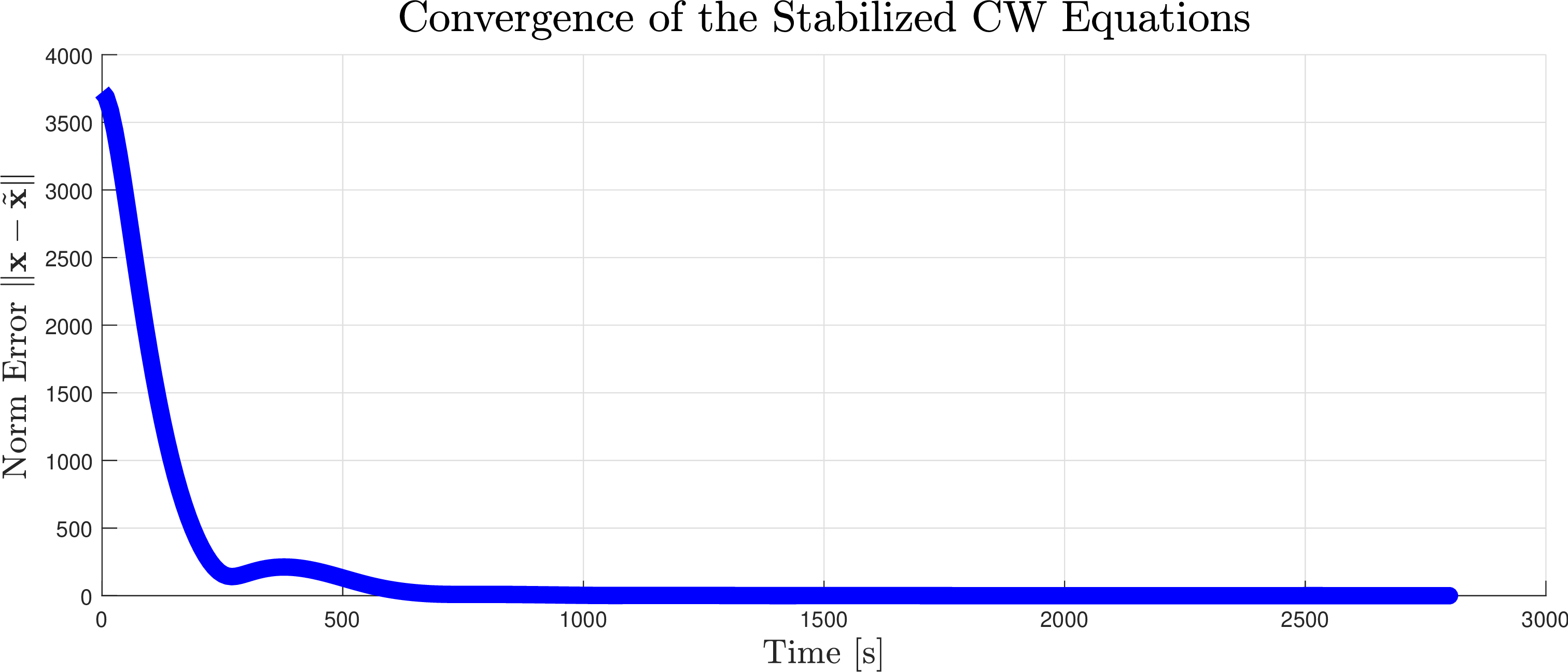
We first simulate the behavior of \(\mathcal{H}_{\text{FO}}\) from the initial condition in 39 . As in Proposition 2 and Theorem 2, our focus is on evaluating how closely the state of the chaser approaches its chosen rendezvous point. We therefore examine the value of \(\|\mathbf{x}(t, j) - \tilde{\mathbf{x}}(t)\|\) as a function of \(t\).
This value over time is plotted in Figure 4, which shows that the chaser satellite converges quite closely to the chosen rendezvous point, despite the perturbations given by \(t \mapsto \mathbf{d}(t)\) and the fact that sub-optimal inputs to the system are used over time. The trajectory shown in Figure 4 represents the typical behavior we saw in our simulations, and it shows the success of feedback optimization for satellite rendezvous. The limiting value of \(\|\mathbf{x}(t, j) - \tilde{\mathbf{x}}(t)\|\) is approximately \(0.082\), while \(\bar{\mathbf{d}} = 5\), which indicates that feedback optimization provides a \(98.4\)% reduction in the magnitude of disturbances faced by the system.
| Value of \(\|\mathbf{x} - \tilde{\mathbf{x}}\|\) | |||
|---|---|---|---|
| \(\theta = -0.25\) | \(\theta = 0.5\) | \(\theta = 1.0\) | |
| \(\kappa = 0.1\) | 0.13 | 0.14 | 0.27 |
| \(\kappa = 0.3\) | 0.19 | 0.15 | 0.31 |
| \(\kappa = 0.5\) | 0.43 | 0.27 | 1.57 |
| \(\kappa = 0.7\) | 0.54 | 2.23 | 4.39 |
| \(\kappa = 0.9\) | 1.22 | 4.32 | 3.53 |
We next consider the perturbed system model \(\mathcal{H}_{\text{FO}}^{\rho}\). For the timers \(\tau_{c}\) and \(\tau_{g}\) we use perturbations of the form \(\theta_{c,\min} = \theta_{c,\max} = \theta_{g, \textrm{comp}} = \theta\) and \(\kappa_c = \kappa_g = \kappa\). The values of \(\theta\) and \(\kappa\) used in simulations are shown in Table 1, along with the asymptotic values of \(\|\mathbf{x}(t, j) - \tilde{\mathbf{x}}(t)\|\) for each run. A second-order regression of these values gives \[\|\mathbf{x}(t, j) - \tilde{\mathbf{x}}(t)\|\approx 0.256 - 1.62\kappa - 0.449\theta + 4.131\kappa^2 - 0.023\theta^2 + 3.364\kappa\theta.\]
Figure 5 shows the behavior of \(\|\mathbf{x}(t, j) - \tilde{\mathbf{x}}(t)\|\) for \(\theta = 1\) and varying values of \(\kappa\). The value \(\theta = 1\) means that the timers \(\tau_{c}\) and \(\tau_{g}\) take one second longer to jump than they do in the nominal system model. The positive values taken by \(\kappa\) mean that both \(\tau_{c}\) and \(\tau_{g}\) count down more slowly than they do in the nominal system model. Figure 6 shows simulations for \(\theta = 0.5\) and varying values of \(\kappa\). Figure 7 does the same for \(\theta = -0.25\) and varying values of \(\kappa\). The negative value of \(\theta\) implies that \(\tau_{c}\) and \(\tau_{g}\) count down to zero faster than they do in the nominal model.
Table 2 gives the asymptotic values of \(\|\mathbf{x}(t, j) - \tilde{\mathbf{x}}(t)\|\) for each value of \(\rho = \max\{\theta, \kappa\}\). Table 2 shows that larger perturbations \(\rho\) produce larger asymptotic errors in the chaser’s state, which is intuitive. Table 1 shows that increasing \(\theta\) increases errors more rapidly than increasing \(\kappa\). Intuitively, smaller values of both \(\theta\) and \(\kappa\) produce smaller errors because computations, measurements of outputs, and changes in the input happen more quickly for those smaller values, which allows the underlying optimization algorithm to react more quickly to disturbances faced by the system.
| Asymptotic value of \(\|\mathbf{x}(t, j) - \tilde{\mathbf{x}}(t)\|\) | |||||
|---|---|---|---|---|---|
| \(\rho\) | 0.1 | 0.3 | 0.5 | 0.7 | 0.9 |
| Value | 0.05 | 0.11 | 0.35 | 2.15 | 4.23 |
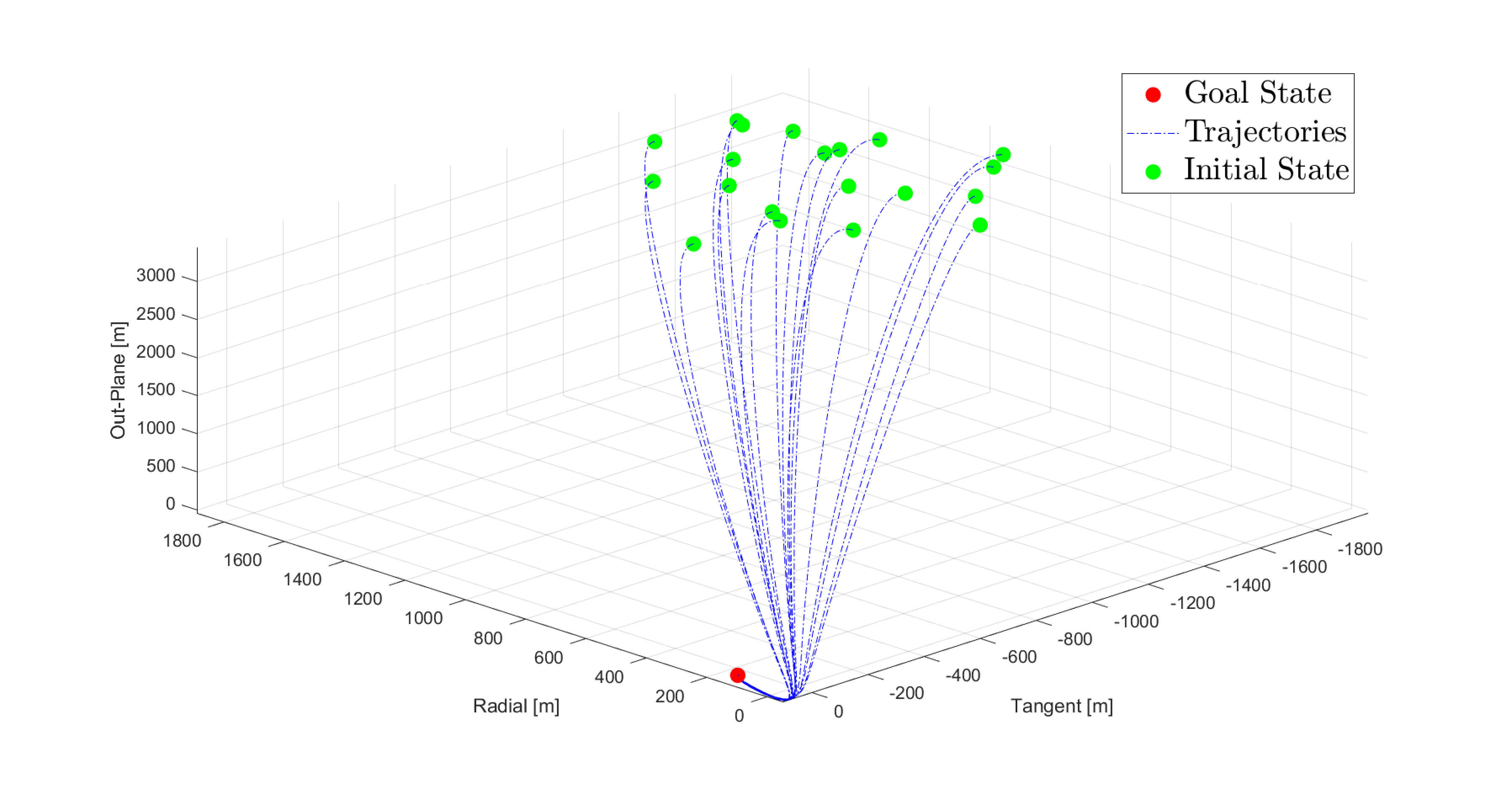
For the third set of simulations we consider \(20\) initial conditions of the nominal system \(\mathcal{H}_{\text{FO}}\) that satisfy \[\begin{gather} \label{eq:initconds2} \mathbf{x}(0,0) \in [1000, 2000] \times [-1000, -2000] \times [-2500, -3500] \times [0.1, 4.0] \times \\ [0.1, 4.0] \times [0.1, 4.0], \mathbf{u}(0,0) = \big(0, 0, 0\big)^\top, ~\mathbf{y}_s(0,0) = \mathbf{x}(0,0) + 5,~\mathbf{z}(0,0) = \big(0, 0, 0\big)^\top,\\ \tau_{c}(0,0) = 0.175,~\tau_{g}(0,0) = 0.5,~\tau_{d}(0,0) = 0, \end{gather}\tag{40}\] and we simulated trajectories from each. Figure 8 shows that all trajectories produce asymptotically small values of \(\|\mathbf{x}(t, j) - \tilde{\mathbf{x}}(t)\|\), with the largest among them being \(0.81\) meters, which illustrates that the feedback optimization approach we use reliably drives the chaser satellite close to its rendezvous point with the target satellite.
8 Conclusion↩︎
This paper developed a hybrid system model for feedback optimization in a satellite rendezvous problem that considers continuous-time dynamics with discrete-time optimization in the loop. The resulting hybrid model was shown to be well-posed, and all of its solutions were shown to be complete and non-Zeno. Analytically, the solutions to this system were shown to converge to a ball around a desired rendezvous point, and in simulation the radius of that ball was shown to be small, indicating close convergence to desired rendezvous points. Future work includes using hybrid feedback optimization for systems with nonlinear dynamics, such as including attitude control with the CW equations.
9 Basic Results on Hybrid Systems↩︎
For completeness we reproduce here two basic results from the study of hybrid systems.
Lemma 3 (Lemma A.33 in [34]). Given closed sets \(D_1\subset \mathbb{R}^m\) and \(D_2\subset \mathbb{R}^m\) and the set-valued maps \(G_1:D_1 \rightrightarrows \mathbb{R}^n\) and \(G_2:D_2\rightrightarrows\mathbb{R}^n\) that are outer semicontinuous and locally bounded relative to \(D_1\) and \(D_2\), respectively, the set-valued map \(G:D\rightrightarrows \mathbb{R}^n\) given by \[G(\zeta) := G_1(\zeta) \cup G_2(\zeta) = \begin{cases} G_1(\zeta) &\text{if } \zeta \in D_1 \backslash D_2 \\ G_2(\zeta) &\text{if } \zeta \in D_2 \backslash D_1\\ G_1(\zeta)\cup G_2(\zeta) &\text{if } \zeta \in D_1 \cap D_2 \end{cases}\label{OSLBjump}\tag{41}\] for each \(\zeta\in D\) is outer-semicontinuous and locally bounded relative to the closed set \(D\).
Lemma 4 (Basic existence of solutions; Proposition 2.34 in [34]). Let \(\mathcal{H}=(C,F,D,G)\) satisfy Definition 1. Take an arbitrary \(\nu \in C \cup D.\) If \(\nu \in D\) or
(VC) there exists a neighborhood \(U\) of \(\nu\) such that for every \(\zeta \in U \cap C\), \[F(\zeta) \cap T_C(\zeta) \neq
\emptyset,\] then there exists a nontrivial solution \(\phi\) to \(\mathcal{H}\) with \(\phi(0,0)=\nu\). If (VC) holds for every \(\nu \in C\backslash D\), then there exists a nontrivial solution to \(\mathcal{H}\) from every initial point in \(C \cup D\), and every maximal solution \(\phi\) to \(\mathcal{H}\) satisfies exactly one of the following conditions:
\(\phi\) is complete;
dom \(\phi\) is bounded and the interval \(I^J\), where \(J = \sup_j \textrm{dom } \phi\), has nonempty interior and \(t\mapsto \phi(t,J)\) is a maximal solution to \(\dot{z}\in F(z)\), in fact lim\(_{t\rightarrow T}|\phi(t,J)|=\infty\), where \(T = \sup_t \textrm{dom } \phi\);
\(\phi(T,J)\in C\cup D\), where \((T,J)= \sup \textrm{dom } \phi\).
Furthermore, if \(G(D)\subset C \cup D\), then \(3)\) above does not occur.
10 Section 5 Proofs↩︎
10.1 Proof of Lemma 1↩︎
For the hybrid model \(\mathcal{H}_{\text{FO}}\) in 24 , the set \(C\) in 17 and the set \(D\) in 18 satisfy Condition [hybridcond95one] in Definition 1 by inspection. The map \(F\) in 19 is defined everywhere on \(C\) and outputs a singleton that is linear in \(\mathbf{x}\), \(\mathbf{u}\), and \(\mathbf{d}\). The disturbance \(\mathbf{d}\) that appears in \(F\) is bounded under Assumption 3, and \(F\) therefore satisfies Condition [hybridcond95two] in Definition 1.
To satisfy Condition [hybridcond95three] for the map \(G\) in 23 , we use Lemma 3 in 9. The jump map \(G_1\) in 20 is outer semicontinuous since the projection mapping \(\Pi_{\mathcal{U}}[\cdot]\) is continuous and all other entries are singletons. The jump map \(G_2\) in 21 is outer semicontinuous since its only set-valued entry is a compact interval and all other entries are singletons. Since the jump map in 23 has the structure of the jump map in Lemma 3 and the jump set in 18 has the structure of the jump set in Lemma 3, we can apply Lemma 3 to the map \(G\) in 23 . Then \(G\) is outer semicontinuous and locally bounded relative to the closed set \(D\). Then Condition [hybridcond95three] of Definition 1 is satisfied. Therefore, all conditions of Definition 1 are satisfied, and \(\mathcal{H}_{\text{FO}}\) is well-posed.
10.2 Proof of Proposition 1↩︎
Since \(\mathcal{H}_{\text{FO}}\) is well-posed as shown in Lemma 1, the results follow from applying Lemma 4 in 9. First we show that the condition (VC) holds for all \(\nu\in C\backslash D\). Consider an arbitrary \(\nu\in C\backslash D\), and let \(U\) be a neighborhood of \(\nu\). We show that \(F(\zeta) \cap T_{C}(\zeta) \neq \emptyset\) for each \(\zeta \in U\cap C\), where \(T_{C}(\zeta)\) is the tangent cone of the set \(C\) at the point \(\zeta\). Based on the flow map \(F\) from 19 , only \(\dot{\mathbf{x}}\), \(\dot{\tau_{c}}\), \(\dot{\tau_{g}}\), and \(\dot{\tau_{d}}\) are non-zero during flows. In addition, \(C\) does not restrict the values of \(\mathbf{x}\) or \(\tau_{d}\), which implies that all values of \(\dot{\mathbf{x}}\) and \(\dot{\tau_{d}}\) are allowable at all values of \(\mathbf{x}\) and \(\tau_{d}\), respectively. On the other hand, the timers \(\tau_{c}\) and \(\tau_{g}\) take values in compact intervals, which implies that some directions are infeasible at some values of \(\tau_{c}\) and \(\tau_{g}\). Therefore, satisfaction of the condition \(F(\zeta)\cap T_C(\zeta) \neq \emptyset\) is determined by the dynamics of \(\tau_{c}\) and \(\tau_{g}\).
To show that \(F(\zeta)\cap T_C(\zeta) \neq \emptyset\), we compute the tangent cone \(T_C(\zeta)\) as \[T_{C}(\zeta) := \begin{cases} \mathbb{R}^{18} \times \{-1\} \times \mathbb{R}\times \mathbb{R}&\text{if \tau_{c} = \tau_{c,\max}} \text{ and \tau_{g} \in (0, \tau_{g,\textrm{comp}})}\\ \mathbb{R}^{18} \times \{-1\} \times \{1\} \times \mathbb{R}&\text{if \tau_{c} = \tau_{c,\max}} \text{ and \tau_{g} = 0}\\ \mathbb{R}^{18}\times \{1\} \times \{-1\} \times \mathbb{R}&\text{if \tau_{c} = 0} \text{ and \tau_{g} = \tau_{g,\textrm{comp}}}\\ \mathbb{R}^{18} \times \mathbb{R}\times \{-1\} \times \mathbb{R}&\text{if \tau_{c} \in (\tau_{c,\min}, \tau_{c,\max})} \text{ and \tau_{g} = \tau_{g,\textrm{comp}}}\\ \mathbb{R}^{18}\times \{-1\} \times \{-1\} \times \mathbb{R}&\text{if \tau_{c} = \tau_{c,\max} } \text{ and \tau_{g} = \tau_{g,\textrm{comp}}}\\ \mathbb{R}^{18} \times \{1\} \times \{1\} \times \mathbb{R}&\text{if \tau_{c} = 0 } \text{ and \tau_{g} = 0}\\ \mathbb{R}^{18} \times \mathbb{R}\times \mathbb{R}\times \mathbb{R}&\text{otherwise.} \end{cases}\] Then \(F(\zeta)\in T_C(\zeta)\) for every \(\zeta \in C \backslash D\) and condition (VC) from Lemma 4 is satisfied for every \(\nu \in C \backslash D\). Then by Lemma 4 there exists a nontrivial solution \(\phi\) to \(\mathcal{H}_{FO}\) with the initial condition \(\phi(0,0) = \nu\). Let \(\mathcal{S}_{\mathcal{H}_{FO}}\) denote the set of all maximal solutions to \(\mathcal{H}_{FO}\). Every solution \(\phi \in \mathcal{S}_{\mathcal{H}_{FO}}\) satisfies one of the three conditions in Lemma 4.
The system \(\mathcal{H}_{\text{FO}}\) satisfies \(G(D) \subset C \cup D\), which implies that \(3)\) in Lemma 4 does not occur. Regarding \(2)\), the only components of the solution that change during flows are \(\mathbf{x}, \tau_{c}\), \(\tau_{g}\), and \(\tau_{d}\). Since \(\tau_{c}\) and \(\tau_{g}\) take values in compact sets, they are bounded and cannot blow up to infinity. Since \(\mathbf{u} \in \mathcal{U}\), which is a compact set, the input \(\mathbf{u}\) is bounded, and there exists some finite \(\mathbf{u}_{max} \geq 0\) such that \(\|\mathbf{u}\| \leq \mathbf{u}_{max}\) for all \(\mathbf{u} \in \mathcal{U}\). Similarly, \(\mathbf{d} \in \mathcal{D}\), which is a compact set, and there exists some \(\mathbf{d}_{max} \geq 0\) such that \(\|\mathbf{d}\| \leq \mathbf{d}_{max}\) for all \(\mathbf{d} \in \mathcal{D}\). Since the mapping \((\mathbf{x}, \mathbf{u}) \mapsto {A}_{\textrm{stab}}\mathbf{x} + B_{\textrm{stab}}\mathbf{u} - B_{\textrm{stab}}K\mathbf{d}\) is globally Lipschitz and both \(\mathbf{u}\) and \(\mathbf{d}\) are bounded, the state \(\mathbf{x}\) does not blow up in finite time. Finally, since \(\dot{\tau_{d}} = 1\), the timer \(\tau_{d}\) cannot blow up in finite time. Then Condition \(2)\) from Lemma 4 does not hold. Therefore, Condition \(1)\) from Lemma 4 holds and all maximal solutions to \(\mathcal{H}_{\text{FO}}\) are complete.
Regarding Zeno behavior, jumps in \(G\) are triggered only when either one of the timers \(\tau_{c}\) or \(\tau_{g}\) has reached zero, and \(G\) resets any timers that have reached zero to non-zero values. This property implies that \(G(D) \cap D = \emptyset\), ruling out Zeno behavior by Proposition 2.34 in [34].
11 Section 6 Proofs↩︎
11.1 Proof of Proposition 2↩︎
In this proof any empty sums evaluate to zero by convention, and we take \(\alpha(-1) = 0\) for notational convenience.
The high-level steps of the proof are:
Bound the distance between the input \(\mathbf{u}\) and the optimal input \(\mathbf{u}^*\).
Give an expression for the difference \(\mathbf{x}(t_{},j{}) - \tilde{\mathbf{x}}(t)\) in terms of integrals of the dynamics of \(x(t, j)\).
Bound each integrand that does not have a closed form integral.
Evaluate each reuslting integral and simplify to bound \(\|\mathbf{x}(t_{},j{}) - \tilde{\mathbf{x}}(t)\|\).
We begin with Step [step:1]. By definition of \(\mathcal{A}(t)\) we have \[\label{eq:t1normsequal} \|\phi(t, j)\|_{\mathcal{A}(t)} = \big\|\mathbf{x}(t_{},j{})\big\|_{\{\tilde{\mathbf{x}}(t)\}} = \big\|\mathbf{x}(t_{},j{}) - \tilde{\mathbf{x}}(t)\big\|.\tag{42}\] We define \(P = \max\{p \in \mathbb{N} : \bar{\alpha}(p) + p \leq j\}\), which is the number of times the input \(\mathbf{u}\) has changed up to jump time \(j\). We now address step [step:1], suppose \(P \geq 1\), then using 28 in 27 we see that for each \(p \in \{1, \ldots, P\}\) we have \(\mathbf{u}(t_{\xi(p,0)},{\xi(p,0)}) = \mathbf{z}_{\alpha({p-1})}(t_{\xi(p-1,\alpha(p-1))},{\xi(p-1,\alpha(p-1))})\). If \(P = 0\), then we have only \(\mathbf{u}(t_{\xi(0,0)},{\xi(0,0)}) = \mathbf{u}(0,0) = \mathbf{z}_{0}(0, 0)\). For \(p \geq 1\) the optimal value for \(\mathbf{u}(t_{\xi(p,0)},{\xi(p,0)})\) is \(\mathbf{u}^*(t_{\xi(p,0)},{\xi(p,0)}) = \mathbf{z}^*(t_{\xi(p-1,0)},{\xi(p-1,0)})\), where we define \(\mathbf{z}^{*}(t_{\xi(p-1,0)},{\xi(p-1,0)}) = \mathop{\mathrm{arg\,min}}\limits_{\mathbf{u} \in \mathcal{U}} \, \Phi\big(\mathbf{u}, \mathbf{y}_{s}(t_{\xi(p-1,0)},{\xi(p-1,0)})\big)\). From Lemma 2 we know that for \(p \geq 1\) \[\begin{gather} \label{eq:thm1951} \big\|\mathbf{z}_{\alpha({p-1})}\big(\xi(p-1,\alpha(p-1))\big) -\mathbf{z}^*(t_{\xi(p-1,0)},{\xi(p-1,0)})\big\| \leq \\ q^{\frac{\alpha({p-1})-1}{2}}\|\mathbf{z}_{1}(t_{\xi(p-1,1)},{\xi(p-1,1)}) - \mathbf{z}^*(t_{\xi(p-1,0)},{\xi(p-1,0)})\big\|. \end{gather}\tag{43}\] For \(p \geq 1\) we also have \[\begin{gather} \label{eq:thm1952} \mathbf{z}_{1}(t_{\xi(p-1,1)},{\xi(p-1,1)}) = \Pi_{\mathcal{U}}\bigg[\mathbf{z}_0(t_{\xi(p-1,0)},{\xi(p-1,0)}) \\ -\gamma\Big(\nabla_{\mathbf{u}} \Phi\big(\mathbf{z}_0(t_{\xi(p-1,0)},{\xi(p-1,0)}), \mathbf{y}_{s}(t_{\xi(p-1,0)},{\xi(p-1,0)})\big) \\ + H^T\nabla_{\mathbf{y}} \Phi\big(\mathbf{z}_0(t_{\xi(p-1,0)},{\xi(p-1,0)}), \mathbf{y}_{s}(t_{\xi(p-1,0)},{\xi(p-1,0)})\big) \Big)\bigg]. \end{gather}\tag{44}\] In projected gradient descent the optimum is a fixed point so that \[\begin{gather} \label{eq:thm1953} \mathbf{z}^*(t_{\xi(p-1,0)},{\xi(p-1,0)}) = \Pi_{\mathcal{U}}\Big[\mathbf{z}^*(t_{\xi(p-1,0)},{\xi(p-1,0)}) \\ -\gamma\Big(\nabla_{\mathbf{u}} \Phi\big(\mathbf{z}^*(t_{\xi(p-1,0)},{\xi(p-1,0)}), \mathbf{y}_{s}(t_{\xi(p-1,0)},{\xi(p-1,0)})\big) \\ + H^T\nabla_{\mathbf{y}} \Phi\big(\mathbf{z}^*(t_{\xi(p-1,0)},{\xi(p-1,0)}), \mathbf{y}_{s}(t_{\xi(p-1,0)},{\xi(p-1,0)})\big) \Big)\bigg]. \end{gather}\tag{45}\] Using the relation \[\mathbf{y}_s(t_{\xi(p-1,0)},{\xi(p-1,0)}) = H_{\textrm{stab}} \mathbf{z}_0(t_{\xi(p-1,0)},{\xi(p-1,0)}) + \mathbf{d}(t_{\xi(p-1,0)})\] from 22 , we combine 43 , 44 , and 45 to find that for \(p \geq 1\), \[\begin{gather} \label{eq:thm1955} \left\|\mathbf{u}(t_{\xi(p,0)},{\xi(p,0)}) - \mathbf{u}^*(t_{\xi(p,0)},{\xi(p,0)})\right\| \leq q^{\frac{\alpha({p-1})-1}{2}} \big\| \mathbf{z}_{0}(t_{\xi(p-1,0)},{\xi(p-1,0)}) \\ -\gamma(Q_{\mathbf{u}} + H_{\textrm{stab}}^{\top}Q_{\mathbf{y}}H_{\textrm{stab}})\mathbf{z}_{0}(t_{\xi(p-1,0)},{\xi(p-1,0)}) - \gamma H_{\textrm{stab}}^\top Q_{\mathbf{y}} (\mathbf{d}(t_{\xi(p-1,0)}) - \hat{\mathbf{y}}) \\ - \mathbf{z}^*(t_{\xi(p-1,0)},{\xi(p-1,0)}) + \gamma\big(Q_{\mathbf{u}} + H_{\textrm{stab}}^TQ_{\mathbf{y}}H_{\textrm{stab}}\big)\mathbf{z}^*(t_{\xi(p-1,0)},{\xi(p-1,0)}) \\ + \gamma H_{\textrm{stab}}^TQ_{\mathbf{y}}(\mathbf{d}(t_{\xi(p-1,0)}) - \hat{\mathbf{y}}) \big\|, \end{gather}\tag{46}\] where we have substituted both \(\mathbf{u}(t_{\xi(p,0)},{\xi(p,0)}) = \mathbf{z}_{\alpha(p-1)}\big(\xi(p-1,\alpha(p-1))\big)\) and \(\mathbf{u}^*(t_{\xi(p,0)},{\xi(p,0)}) = \mathbf{z}^*(t_{\xi(p-1,0)},{\xi(p-1,0)})\). We have also used the non-expansive property of \(\Pi_{\mathcal{U}}\), namely that \(\|\Pi_{\mathcal{U}}[u_1] - \Pi_{\mathcal{U}}[u_2]\| \leq \|u_1 - u_2\|\) for all \(u_1, u_2 \in \mathcal{U}\). Combining like terms and applying the triangle inequality gives \[\begin{gather} \left\|\mathbf{u}(t_{\xi(p,0)},{\xi(p,0)}) - \mathbf{u}^*(t_{\xi(p,0)},{\xi(p,0)})\right\| \leq q^{\frac{\alpha({p-1})-1}{2}} \Big\| \mathbf{z}_{0}(t_{\xi(p-1,0)},{\xi(p-1,0)}) \\ - \mathbf{z}^*(t_{\xi(p-1,0)},{\xi(p-1,0)}) \Big\| \cdot \Big\|I_3 - \gamma(Q_{\mathbf{u}} + H_{\textrm{stab}}^TQ_{\mathbf{y}}H_{\textrm{stab}})\Big\| \end{gather}\] for \(p \geq 1\). We have \(\|\mathbf{z}_{0}(t_{\xi(p-1,0)},{\xi(p-1,0)}) - \mathbf{z}^*(t_{\xi(p-1,0)},{\xi(p-1,0)})\| \leq d_{\mathcal{U}}\) by definition of \(d_{\mathcal{U}}\), and a straightforward calculation shows \(\|I_3 - \gamma(Q_{\mathbf{u}} + H_{\textrm{stab}}^TQ_{\mathbf{y}}H_{\textrm{stab}})\| \leq q^{\frac{1}{2}}\). Then \[\left\|\mathbf{u}(t_{\xi(p,0)},{\xi(p,0)}) - \mathbf{u}^*(t_{\xi(p,0)},{\xi(p,0)})\right\| \leq q^{\frac{\alpha({p-1})}{2}} d_{\mathcal{U}} \label{eq:u95convergence}\tag{47}\] for each \(p \geq 1\).
We now move to Step [step:2]. The model of \(\mathcal{H}_{FO}\) applies piecewise constant inputs to the underlying chaser dynamics. We therefore integrate the chaser’s dynamics over the intervals with constant inputs and compute the distance between \(\mathbf{x}(t, j)\) and \(\tilde{\mathbf{x}}(t)\) for an arbitrary \((t, j) \in \textrm{dom }\phi\). For each \(p \in \{0, \ldots, P\}\) the input is equal to \(\mathbf{u}(t_{\xi(p,0)},{\xi(p,0)})\) over intervals of the form \([t_{\xi(p,0)}, t_{\xi(p+1,0)}]\), and therefore we may write \[\begin{gather} \label{eq:thm195951} \mathbf{x}(t, j) - \tilde{\mathbf{x}}(t) = \exp(A_{\textrm{stab}}t)\mathbf{x}({0},{0}) + \sum^{P-1}_{p=0}\int_{t_{\xi(p,0)}}^{t_{\xi(p+1,0)}} \!\!\!\!\!\!\!\!\!\!\exp\big(A_{\textrm{stab}}(t_{\xi(p+1,0)}-\tau)\big) d\tau \\ \cdot B_{\textrm{stab}}\mathbf{u}(t_{\xi(p,0)},{\xi(p,0)}) + \int_{t_{\xi(P,0)}}^{t} \exp\big(A_{\textrm{stab}}(t - \tau)\big) d\tau B_{\textrm{stab}}\mathbf{u}(t_{\xi(P,0)},{\xi(P,0)}) \\ - A_{\textrm{stab}}^{-1}B_{\textrm{stab}}K\mathbf{d}(t) + A_{\textrm{stab}}^{-1}B_{\textrm{stab}}\tilde{\mathbf{u}}(t) - \int^{t}_{0}\exp\big(A_{\textrm{stab}}(t - \tau)\big)B_{\textrm{stab}}K\mathbf{d}(\tau)d\tau, \end{gather}\tag{48}\] where \(\tilde{\mathbf{x}}(t) = A_{\textrm{stab}}^{-1}B_{\textrm{stab}}K\mathbf{d}(t) - A_{\textrm{stab}}^{-1}B_{\textrm{stab}}\tilde{\mathbf{u}}(t)\) is from 31 . Next, using integration by parts, we find \[\begin{gather} \label{eq:integrationbyparts} - \int^{t}_{0}\exp\big(A_{\textrm{stab}}(t - \tau)\big)B_{\textrm{stab}}K\mathbf{d}(\tau)d\tau = A_{\textrm{stab}}^{-1}B_{\textrm{stab}}K\mathbf{d}(t)\\ - \exp\big(A_{\textrm{stab}}t\big)A_{\textrm{stab}}^{-1}B_{\textrm{stab}}K\mathbf{d}(0) - \int^{t}_{0}\exp\big(A_{\textrm{stab}}(t - \tau)\big)A_{\textrm{stab}}^{-1}B_{\textrm{stab}}K\dot{\mathbf{d}}(\tau)d\tau. \end{gather}\tag{49}\] We use 49 in 48 and add and subtract the term \[\begin{gather} \sum_{p=0}^{P-1} \int_{t_{\xi(p,0)}}^{t_{\xi(p+1,0)}} \exp\big(A_{\textrm{stab}}(t_{\xi(p+1,0)} - \tau)\big)d\tau B_{\textrm{stab}} \mathbf{u}^*(t_{\xi(p,0)},{\xi(p,0)}) \\ + \int_{t_{\xi(P,0)}}^{t} \exp\big(A_{\textrm{stab}}(t - \tau)\big)d\tau B_{\textrm{stab}}\mathbf{u}^*(t_{\xi(P,0)},{\xi(P,0)}) \\ + \int_0^t \exp\big(A_{\textrm{stab}}(t - \tau)\big)d\tau B_{\textrm{stab}} \tilde{\mathbf{u}}(t) + \exp(A_{\textrm{stab}}t)B_{\textrm{stab}}K\mathbf{d}(t) \end{gather}\] to find \[\begin{gather} \mathbf{x}(t, j) - \tilde{\mathbf{x}}(t) = \exp(A_{\textrm{stab}}t)\mathbf{x}({0},{0}) \\ + \sum^{P-1}_{p=0}\int_{t_{\xi(p,0)}}^{t_{\xi(p+1,0)}} \exp\big(A_{\textrm{stab}}(t_{\xi(p+1,0)}-\tau)\big) d\tau B_{\textrm{stab}}\big(\mathbf{u}(t_{\xi(p,0)},{\xi(p,0)}) \\ - \mathbf{u}^*(t_{\xi(p,0)},{\xi(p,0)})\big) + \int_{t_{\xi(P,0)}}^{t} \exp\big(A_{\textrm{stab}}(t - \tau)\big) d\tau B_{\textrm{stab}} \big( \mathbf{u}(t_{\xi(P,0)},{\xi(P,0)}) \\ - \mathbf{u}^*(t_{\xi(p,0)},{\xi(p,0)})\big) + \sum^{P-1}_{p=0}\int_{t_{\xi(p,0)}}^{t_{\xi(p+1,0)}} \exp\big(A_{\textrm{stab}}(t_{\xi(p+1,0)}-\tau)\big) d\tau B_{\textrm{stab}} \\ \cdot \big(\mathbf{u}^*(t_{\xi(p,0)},{\xi(p,0)}) - \tilde{\mathbf{u}}(t)\big) \!\!+ \! \int_{t_{\xi(P,0)}}^{t} \!\!\!\!\!\!\!\exp\big(A_{\textrm{stab}}(t - \tau)\big) d\tau B_{\textrm{stab}}\big(\mathbf{u}^*(t_{\xi(P,0)},{\xi(P,0)}) \\ - \tilde{\mathbf{u}}(t)\big) + \exp\big(A_{\textrm{stab}}t\big)A_{\textrm{stab}}^{-1}B_{\textrm{stab}}\tilde{\mathbf{u}}(t) -\exp\big(A_{\textrm{stab}}t\big)A_{\textrm{stab}}^{-1}B_{\textrm{stab}}K\mathbf{d}(0) \\ - \int^{t}_{0} \exp\big(A_{\textrm{stab}}(t - \tau)\big)A_{\textrm{stab}}^{-1}B_{\textrm{stab}}K\dot{\mathbf{d}}(\tau)d\tau, \end{gather}\] where we have also used \(\int_{0}^{t} \exp\big(A_{\textrm{stab}}(t - \tau)\big) d\tau = \Big(\exp\big(A_{\textrm{stab}}t\big) - I_{6}\Big)A_{\textrm{stab}}^{-1}\). After taking the norm of \(\mathbf{x}(t, j) - \tilde{\mathbf{x}}(t)\) we use \[\int^{t}_{0} \exp\big(A_{\textrm{stab}}t\big)A_{\textrm{stab}}^{-1}B_{\textrm{stab}}K\dot{\mathbf{d}}(\tau)d\tau = \exp\big(A_{\textrm{stab}}t\big)A_{\textrm{stab}}^{-1}B_{\textrm{stab}}K\big(\mathbf{d}(t) - \mathbf{d}(0)\big)\] and \(\tilde{\mathbf{x}}(t) = -A_{\textrm{stab}}^{-1}B_{\textrm{stab}}\tilde{\mathbf{u}}(t) + A_{\textrm{stab}}^{-1}B_{\textrm{stab}} K \mathbf{d}(t)\), and then we apply the triangle inequality to find \[\begin{gather} \big\|\mathbf{x}(t, j) - \tilde{\mathbf{x}}(t) \big\| \leq \big\|\exp(A_{\textrm{stab}}t)\big\|\big\|\mathbf{x}({0},{0}) - \tilde{\mathbf{x}}(t) \big\| \\ + \frac{1}{m_{c}}\sum^{P-1}_{p=0}\int_{t_{\xi(p,0)}}^{t_{\xi(p+1,0)}} \big\|\exp\big(A_{\textrm{stab}}(t_{\xi(p+1,0)}-\tau)\big)\big\| d\tau \big\|\mathbf{u}(t_{\xi(p,0)},{\xi(p,0)}) \\ - \mathbf{u}^*(t_{\xi(p,0)},{\xi(p,0)}) \big\| + \frac{1}{m_{c}}\int_{t_{\xi(P,0)}}^{t} \big\|\exp\big(A_{\textrm{stab}}(t - \tau)\big)\big\| d\tau \big\| \mathbf{u}(t_{\xi(P,0)},{\xi(P,0)}) \\ - \mathbf{u}^*(t_{\xi(p,0)},{\xi(p,0)}) \big\| + \frac{1}{m_{c}}\sum^{P-1}_{p=0}\int_{t_{\xi(p,0)}}^{t_{\xi(p+1,0)}} \big\|\exp\big(A_{\textrm{stab}}(t_{\xi(p+1,0)}-\tau)\big)\big\| d\tau \\ \cdot \big\|\mathbf{u}^*(t_{\xi(p,0)},{\xi(p,0)}) - \tilde{\mathbf{u}}(t)\big\| + \frac{1}{m_{c}}\int_{t_{\xi(P,0)}}^{t} \big\|\exp\big(A_{\textrm{stab}}(t - \tau)\big)\big\| d\tau \big\|\mathbf{u}^*(t_{\xi(P,0)},{\xi(P,0)}) \\ - \tilde{\mathbf{u}}(t)\big\| + \frac{1}{m_{c}}\int^{t}_{0} \big\|\exp\big(A_{\textrm{stab}}t\big) - \exp\big(A_{\textrm{stab}}(t - \tau)\big)\big\|\big\|A_{\textrm{stab}}^{-1}\big\| \big\|K\big\|\big\|\dot{\mathbf{d}}(\tau)\big\|d\tau, \end{gather}\] where we have used \(\big\|B_{\textrm{stab}}\big\| = \frac{1}{m_{c}}\), which is a property of the CW equations that follows from \(B_{\textrm{stab}}^TB_{\textrm{stab}} = \frac{1}{m_c^2}I_3\).
Now we turn to Step [step:2point5]. From Assumption 3 we have \(\big\|\dot{\mathbf{d}}(t)\big\| \leq \bar{\mathbf{d}}\), and since \(\mathcal{U}\) is compact we have \(\|u_1 - u_2\| \leq d_{\mathcal{U}}\) for all \(u_1, u_2 \in \mathcal{U}\). Using these facts and 47 gives \[\begin{gather} \label{eq:thm1957} \big\|\mathbf{x}(t, j) - \tilde{\mathbf{x}}(t) \big\| \leq \big\|\exp(A_{\textrm{stab}}t)\big\|\big\|\mathbf{x}({0},{0}) - \tilde{\mathbf{x}}(t)\big\| \\ + \frac{1}{m_{c}}\int_{0}^{t_{\xi(1,0)}} \big\|\exp\big(A_{\textrm{stab}}(t_{\xi(1,0)}-\tau)\big)\big\| d\tau \; d_{\mathcal{U}}\\ + \frac{1}{m_{c}}\sum^{P-1}_{p=1}\int_{t_{\xi(p,0)}}^{t_{\xi(p+1,0)}} \big\|\exp\big(A_{\textrm{stab}}(t_{\xi(p+1,0)}-\tau)\big)\big\| d\tau q^{\frac{\alpha({p-1})}{2}} \; d_{\mathcal{U}} \\ + \frac{1}{m_{c}}\int_{t_{\xi(P,0)}}^{t} \big\|\exp\big(A_{\textrm{stab}}(t - \tau)\big)\big\| d\tau \; q^{\frac{\alpha({P-1})}{2}} d_{\mathcal{U}} + \frac{1}{m_{c}}\int_{0}^{t} \big\|\exp\big(A_{\textrm{stab}}(t - \tau)\big)\big\| d\tau \; d_{\mathcal{U}}\\ + \frac{1}{m_{c}}\int^{t}_{0} \big\|\exp\big(A_{\textrm{stab}}t\big) - \exp\big(A_{\textrm{stab}}(t - \tau)\big)\big\|d\tau \big\|A_{\textrm{stab}}^{-1}\big\|\big\|K\big\|\bar{\mathbf{d}}, \end{gather}\tag{50}\] where we have combined integrals, separated the \(p = 0\) term from the sum, and used \(\alpha(-1) = 0\). The last integrand can be bounded via \[\begin{align} \big\|\exp\big(A_{\textrm{stab}}t\big) - \exp\big(A_{\textrm{stab}}(t - \tau)\big)\big\| &\leq \big\|\exp\big(A_{\textrm{stab}}(t - \tau)\big\|\big\|\exp\big(A_{\textrm{stab}}\tau\big) - I_6\big\| \\ &\leq \big\|\exp\big(A_{\textrm{stab}}(t - \tau)\big)\big\|\big(\big\|\exp\big(A_{\textrm{stab}}\tau\big)\big\| + 1\big). \label{eq:thm195952} \end{align}\tag{51}\] From [36], we have \[\label{eq:thm1959} \big\|\exp(A_{\textrm{stab}}t)\big\| \leq \mu_{\max}(\Lambda_{\textrm{des}}) \frac{|\lambda_6|}{|\lambda_1|} \exp\big({-|\lambda_1|}t\big),\tag{52}\] which comes directly from the stabilized CW equations that we study. Using this bound with 51 gives \[\begin{gather} \label{eq:thm195953} \int^{t}_{0} \big\|\exp\big(A_{\textrm{stab}}t\big) - \exp\big(A_{\textrm{stab}}(t - \tau)\big) \big\|d\tau \leq \mu_{\max}(\Lambda_{\textrm{des}})^2 \Bigg(\frac{|\lambda_6|}{|\lambda_1|}\Bigg)^2t\exp\big({-|\lambda_1|}t\big) \\ + \mu_{\max}(\Lambda_{\textrm{des}}) \frac{|\lambda_6|}{|\lambda_1|} \int^{t}_{0}\exp\big({-|\lambda_1|}(t - \tau)\big)d\tau. \end{gather}\tag{53}\] Assumption 2 ensures \(\alpha(p) \geq \ell\) for all \(p \in \mathbb{N}\). Since \(q\in (0,1)\), we have \(q^{\frac{\alpha({p-1})}{2}} \leq q^{\frac{\ell}{2}}\) for all \(p \geq 1\).
Now we address Step [step:3]. Using 53 in 50 , evaluating the integrals, and combining with 52 and 53 gives \[\begin{gather} \label{eq:secondbigone} \big\|\mathbf{x}(t, j) - \tilde{\mathbf{x}}(t) \big\| \leq \mu_{\max}(\Lambda_{\textrm{des}})\frac{|\lambda_6|}{|\lambda_1|} \exp\big({-\big|\lambda_{1}\big|}t\big)\big\|\mathbf{x}({0},{0}) - \tilde{\mathbf{x}}(t)\big\| \\ + \frac{\mu_{\max}(\Lambda_{\textrm{des}})\frac{|\lambda_6|}{|\lambda_1|}d_{\mathcal{U}}}{m_{c}\big|\lambda_{1}\big|}\Big[1-\exp\big({-\big|\lambda_{1}\big|}t_{\xi(1,0)}\big)\Big] \\ + \frac{\mu_{\max}(\Lambda_{\textrm{des}})\frac{|\lambda_6|}{|\lambda_1|} q^{\frac{\ell}{2}} d_{\mathcal{U}} }{m_{c}\big|\lambda_{1}\big|} \Big[1-\exp\big({-\big|\lambda_{1}\big|}(t - t_{\xi(1,0)})\big)\Big] \\ + \frac{\mu_{\max}(\Lambda_{\textrm{des}})\frac{|\lambda_6|}{|\lambda_1|}d_{\mathcal{U}} }{m_{c}\big|\lambda_{1}\big|} \Big[1-\exp\big({-\big|\lambda_{1}\big|}t\big)\Big]\\ + \frac{\mu_{\max}(\Lambda_{\textrm{des}})^2\Big(\frac{|\lambda_6|}{|\lambda_1|}\Big)^2}{m_{c}}\big\|A_{\textrm{stab}}^{-1}\big\|\big\|K\big\|\bar{\mathbf{d}}t\exp\big({-|\lambda_1|}t\big) \\ + \frac{\mu_{\max}(\Lambda_{\textrm{des}}) \frac{|\lambda_6|}{|\lambda_1|}}{m_{c}|\lambda_1|}\big\|A_{\textrm{stab}}^{-1}\big\|\big\|K\big\|\bar{\mathbf{d}} \Big[1-\exp\big({-\big|\lambda_{1}\big|}t\big)\Big]. \end{gather}\tag{54}\] Next, using \(\tau_{c,\min} \leq t_{\xi(1,0)} \leq \tau_{c,\max}\) gives the upper bound \[\begin{gather} \label{eq:thm19595953} \big\|\mathbf{x}(t, j) - \tilde{\mathbf{x}}(t) \big\| \leq \mu_{\max}(\Lambda_{\textrm{des}})\frac{|\lambda_6|}{|\lambda_1|} \exp\big({-\big|\lambda_{1}\big|}t\big)\big\|\mathbf{x}({0},{0}) - \tilde{\mathbf{x}}(t)\big\| \\ + \frac{\mu_{\max}(\Lambda_{\textrm{des}})\frac{|\lambda_6|}{|\lambda_1|}d_{\mathcal{U}}}{m_{c}\big|\lambda_{1}\big|}\Big[1-\exp\big({-\big|\lambda_{1}\big|}\tau_{c,\max}\big)\Big] \\ + \frac{\mu_{\max}(\Lambda_{\textrm{des}})\frac{|\lambda_6|}{|\lambda_1|} q^{\frac{\ell}{2}} d_{\mathcal{U}}}{m_{c}\big|\lambda_{1}\big|}\Big[1 - \exp\big({-\big|\lambda_{1}\big|}(t - \tau_{c,\min})\big)\Big] \\ + \frac{\mu_{\max}(\Lambda_{\textrm{des}}) \frac{|\lambda_6|}{|\lambda_1|}d_{\mathcal{U}}}{m_{c}|\lambda_1|}\Big[1-\exp\big({-\big|\lambda_{1}\big|}t\big)\Big]\\ + \frac{\mu_{\max}(\Lambda_{\textrm{des}})^2\Big(\frac{|\lambda_6|}{|\lambda_1|}\Big)^2}{m_{c}}\big\|A_{\textrm{stab}}^{-1}\big\|\big\|K\big\|\bar{\mathbf{d}}t\exp\big({-|\lambda_1|}t\big) \\ + \frac{\mu_{\max}(\Lambda_{\textrm{des}}) \frac{|\lambda_6|}{|\lambda_1|}}{m_{c}|\lambda_1|}\big\|A_{\textrm{stab}}^{-1}\big\|\big\|K\big\|\bar{\mathbf{d}} \Big[1-\exp\big({-\big|\lambda_{1}\big|}t\big)\Big]. \end{gather}\tag{55}\] By factoring we see that \[\label{eq:thm19595954} \exp\big({-\big|\lambda_{1}\big|}(t - \tau_{c,\min}\big) = \exp\big({\big|\lambda_{1}\big|}\tau_{c,\min}\big)\exp\big({-\big|\lambda_{1}\big|}t\big).\tag{56}\] By definition of \(\|\cdot\|_{\mathcal{A}(t)}\), it holds that \[\label{eq:thm19514} \|x(0, 0) - \tilde{x}(t)\| = \|\phi(0, 0)\|_{\mathcal{A}(t)},\tag{57}\] and combining 42 , 55 , 56 and 57 gives \[\begin{gather} \label{eq:thm19517} \|\phi(t, j)\|_{\mathcal{A}(t)} \leq \mu_{\max}(\Lambda_{\textrm{des}})\frac{|\lambda_6|}{|\lambda_1|}\exp\big({-\big|\lambda_{1}\big|}t\big) \big\|\phi({0},{0})\big\|_{\mathcal{A}(t)}\\ + \frac{\mu_{\max}(\Lambda_{\textrm{des}})\frac{|\lambda_6|}{|\lambda_1|}d_{\mathcal{U}}}{m_{c}\big|\lambda_{1}\big|}\big[2 - \exp(-|\lambda_1|\tau_{c,\max}) -\exp\big({-\big|\lambda_{1}\big|}t\big)\big] \\ + \frac{\mu_{\max}(\Lambda_{\textrm{des}})\frac{|\lambda_6|}{|\lambda_1|} q^{\frac{\ell}{2}} d_{\mathcal{U}}}{m_{c}\big|\lambda_{1}\big|}\Big[1 - \exp\big({\big|\lambda_{1}\big|}\tau_{c,\min}\big)\exp\big({-\big|\lambda_{1}\big|}t\big)\Big] \\ + \frac{\mu_{\max}(\Lambda_{\textrm{des}}) \frac{|\lambda_6|}{|\lambda_1|}}{m_{c}|\lambda_1|}\big\|A_{\textrm{stab}}^{-1}\big\|\big\|K\big\|\bar{\mathbf{d}} \Big[1 + \big(\mu_{\max}(\Lambda_{\textrm{des}})|\lambda_6|t - 1\big)\exp\big({-\big|\lambda_{1}\big|}t\big)\Big]. \end{gather}\tag{58}\] Then \[\begin{gather} \limsup_{t+j \rightarrow \infty} \|\phi(t, j)\|_{\mathcal{A}(t)} \leq \mu_{\max}(\Lambda_{\textrm{des}})\frac{|\lambda_6|}{m_{c}|\lambda_1|^2} \cdot \\ \big(2d_{\mathcal{U}} -d_{\mathcal{U}}\exp({-\big|\lambda_{1}\big|}\tau_{c,\max}) + d_{\mathcal{U}}q^{\frac{\ell}{2}} + \big\|A_{\textrm{stab}}^{-1}\big\|\big\|K\big\|\bar{\mathbf{d}}\big). \end{gather}\]
11.2 Proof of Theorem 2↩︎
In this proof any empty sums evaluate to zero by convention, and we take \(\alpha(-1) = 0\) for notational convenience. An arbitrary initial condition \(\phi(0, 0)\) allows for arbitrary \(\mathbf{z}_{0}({0},{0}) \in \mathcal{U}\), \(\tau_{g}(0, 0) \in [0,\tau_{g,\textrm{comp}}]\), and \(\tau_{c}(0,0) \in [0,\tau_{c,\max}]\). In particular, the timer \(\tau_{c}\) can reach zero for the first time before the timer \(\tau_{g}\) reaches zero \(\ell\) times, and the bound in Proposition 2 does not apply to such cases. If that scenario does occur, then \(\tau_{c}\) is reset to a value in the interval \([\tau_{c,\min}, \tau_{c,\max}]\). After that reset, Assumption 2 ensures that \(\tau_{g}\) reaches zero at least \(\ell\) times before \(\tau_{c}\) reaches zero again. Then at least \(\ell\) gradient descent iterations will have been performed before the input \(\mathbf{u}\) changes for the second time. The second change in \(\mathbf{u}\) occurs at hybrid time \((t_{\xi(2,0)},\xi(2,0))\), and we next characterize the behavior of \(\mathcal{H}_{\text{FO}}\) up to that hybrid time.
The input over the interval \([0, t_{\xi(1,0)}]\) is \(\mathbf{u}(0,0)\), and to derive a worst-case bound we suppose that zero gradient descent iterations are performed before the first jump in \(\tau_{c}\). Then \(\mathbf{u}(t_{\xi(1,0)}, \xi(1,0)) = \mathbf{u}(0, 0)\) because no computations have been performed to change the input. Then \(\mathbf{u}(0, 0)\) is the input to the system over the interval \([0, t_{\xi(2,0)}]\). We know that \(\tau_{c,\min}\leq t_{\xi(2,0)} \leq 2\tau_{c,\max}\) because, by continuous time \(t_{\xi(2,0)}\), the timer \(\tau_{c}\) has reached zero from its initial condition in \([0,\tau_{c,\max}]\), then reset to some value in \([\tau_{c,\min}, \tau_{c,\max}]\), then reached zero again.
Repeating the same steps used to reach 50 , using \(\alpha(p) \geq \ell\) for all \(p \geq 2\), and combining integrals we find \[\begin{gather} \label{eq:thm2951} \big\|\mathbf{x}(t, j) - \tilde{\mathbf{x}}(t) \big\| \leq \big\|\exp(A_{\textrm{stab}}t)\big\|\big\|\mathbf{x}({0},{0}) - \tilde{\mathbf{x}}(t)\big\| \\ + \frac{1}{m_{c}}\int_{0}^{t_{\xi(2,0)}} \big\|\exp\big(A_{\textrm{stab}}(t_{\xi(2,0)} - \tau)\big)\big\| d\tau \; d_{\mathcal{U}} \\ + \frac{1}{m_{c}}\int_{t_{\xi(2,0)}}^{t} \big\|\exp\big(A_{\textrm{stab}}(t - \tau)\big)\big\| d\tau \; q^{\frac{\ell}{2}} d_{\mathcal{U}} \\ + \frac{1}{m_{c}}\int_{0}^{t} \big\|\exp\big(A_{\textrm{stab}}(t - \tau)\big)\big\| d\tau d_{\mathcal{U}}\\ + \frac{1}{m_{c}}\int^{t}_{0} \big\|\exp\big(A_{\textrm{stab}}t\big) - \exp\big(A_{\textrm{stab}}(t - \tau)\big)\big\|d\tau \big\|A_{\textrm{stab}}^{-1}\big\|\big\|K\big\|\bar{\mathbf{d}}, \end{gather}\tag{59}\] where the first integral does not have a factor of \(q^{\frac{\ell}{2}}\) in it in order to account for the case in which zero gradient descent iterations are performed before the first jump in \(\mathbf{u}\).
Using 52 and 53 in 59 gives \[\begin{gather} \label{eq:thm295951} \big\|\mathbf{x}(t, j) - \tilde{\mathbf{x}}(t) \big\| \leq \mu_{\max}(\Lambda_{\textrm{des}})\frac{|\lambda_6|}{|\lambda_1|} \exp\big({-\big|\lambda_{1}\big|}t\big)\big\|\mathbf{x}({0},{0}) - \tilde{\mathbf{x}}(t)\big\| \\ + \frac{\mu_{\max}(\Lambda_{\textrm{des}})\frac{|\lambda_6|}{|\lambda_1|}d_{\mathcal{U}}}{m_{c}\big|\lambda_{1}\big|}\Big[1-\exp\big({-\big|\lambda_{1}\big|}t_{\xi(2,0)}\big)\Big] \\ + \frac{\mu_{\max}(\Lambda_{\textrm{des}})\frac{|\lambda_6|}{|\lambda_1|} q^{\frac{\ell}{2}} d_{\mathcal{U}}}{m_{c}\big|\lambda_{1}\big|}\Big[1 - \exp\big({-\big|\lambda_{1}\big|}(t - t_{\xi(2,0)})\big)\Big] \\ + \frac{\mu_{\max}(\Lambda_{\textrm{des}}) \frac{|\lambda_6|}{|\lambda_1|}d_{\mathcal{U}}}{m_{c}|\lambda_1|}\Big[1-\exp\big({-\big|\lambda_{1}\big|}t\big)\Big] \\ + \frac{\mu_{\max}(\Lambda_{\textrm{des}})^2\Big(\frac{|\lambda_6|}{|\lambda_1|}\Big)^2}{m_{c}}\big\|A_{\textrm{stab}}^{-1}\big\|\big\|K\big\|\bar{\mathbf{d}}t\exp\big({-|\lambda_1|}t\big) \\ + \frac{\mu_{\max}(\Lambda_{\textrm{des}}) \frac{|\lambda_6|}{|\lambda_1|}}{m_{c}|\lambda_1|}\big\|A_{\textrm{stab}}^{-1}\big\|\big\|K\big\|\bar{\mathbf{d}} \Big[1-\exp\big({-\big|\lambda_{1}\big|}t\big)\Big]. \end{gather}\tag{60}\] Next, using \(\tau_{c,\min} \leq t_{\xi(2,0)} \leq 2\tau_{c,\max}\) gives the upper bound \[\begin{gather} \label{eq:thm2953} \big\|\mathbf{x}(t, j) - \tilde{\mathbf{x}}(t) \big\| \leq \mu_{\max}(\Lambda_{\textrm{des}})\frac{|\lambda_6|}{|\lambda_1|} \exp\big({-\big|\lambda_{1}\big|}t\big)\big\|\mathbf{x}({0},{0}) - \tilde{\mathbf{x}}(t)\big\| \\ + \frac{\mu_{\max}(\Lambda_{\textrm{des}})\frac{|\lambda_6|}{|\lambda_1|}d_{\mathcal{U}}}{m_{c}\big|\lambda_{1}\big|}\Big[1-\exp\big({-2\big|\lambda_{1}\big|}\tau_{c,\max}\big)\Big] \\ + \frac{\mu_{\max}(\Lambda_{\textrm{des}})\frac{|\lambda_6|}{|\lambda_1|} q^{\frac{\ell}{2}} d_{\mathcal{U}}}{m_{c}\big|\lambda_{1}\big|}\Big[1 - \exp\big({-\big|\lambda_{1}\big|}(t - \tau_{c,\min})\big)\Big] \\ + \frac{\mu_{\max}(\Lambda_{\textrm{des}}) \frac{|\lambda_6|}{|\lambda_1|}d_{\mathcal{U}}}{m_{c}|\lambda_1|}\Big[1-\exp\big({-\big|\lambda_{1}\big|}t\big)\Big]\\ + \frac{\mu_{\max}(\Lambda_{\textrm{des}})^2\Big(\frac{|\lambda_6|}{|\lambda_1|}\Big)^2}{m_{c}}\big\|A_{\textrm{stab}}^{-1}\big\|\big\|K\big\|\bar{\mathbf{d}}t\exp\big({-|\lambda_1|}t\big) \\ + \frac{\mu_{\max}(\Lambda_{\textrm{des}}) \frac{|\lambda_6|}{|\lambda_1|}}{m_{c}|\lambda_1|}\big\|A_{\textrm{stab}}^{-1}\big\|\big\|K\big\|\bar{\mathbf{d}} \Big[1-\exp\big({-\big|\lambda_{1}\big|}t\big)\Big]. \end{gather}\tag{61}\] Combining 42 , 56 , 57 , and 61 gives \[\begin{gather} \label{eq:thm295952} \|\phi(t, j)\|_{\mathcal{A}(t)} \leq \mu_{\max}(\Lambda_{\textrm{des}})\frac{|\lambda_6|}{|\lambda_1|}\exp\big({-\big|\lambda_{1}\big|}t\big) \big\|\phi({0},{0})\big\|_{\mathcal{A}(t)}\\ + \frac{\mu_{\max}(\Lambda_{\textrm{des}})\frac{|\lambda_6|}{|\lambda_1|}d_{\mathcal{U}}}{m_{c}\big|\lambda_{1}\big|}\big[2 - \exp(-2|\lambda_1|\tau_{c,\max}) -\exp\big({-\big|\lambda_{1}\big|}t\big)\big] \\ + \frac{\mu_{\max}(\Lambda_{\textrm{des}})\frac{|\lambda_6|}{|\lambda_1|} q^{\frac{\ell}{2}} d_{\mathcal{U}}}{m_{c}\big|\lambda_{1}\big|}\Big[1 - \exp\big({\big|\lambda_{1}\big|}\tau_{c,\min}\big)\exp\big({-\big|\lambda_{1}\big|}t\big)\Big] \\ + \frac{\mu_{\max}(\Lambda_{\textrm{des}}) \frac{|\lambda_6|}{|\lambda_1|}}{m_{c}|\lambda_1|}\big\|A_{\textrm{stab}}^{-1}\big\|\big\|K\big\|\bar{\mathbf{d}} \Big[1 + \big(\mu_{\max}(\Lambda_{\textrm{des}})|\lambda_6|t - 1\big)\exp\big({-\big|\lambda_{1}\big|}t\big)\Big], \end{gather}\tag{62}\] and the asymptotic result follows by taking the limit superior.
References↩︎
School of Electrical and Computer Engineering, Georgia Institute of Technology, Atlanta, GA, USA 30332. Emails:
{ochuy3,matthale}@gatech.edu.↩︎Space Vehicles Directorate, Air Force Research Laboratory, Kirtland AFB, NM, USA 87108. Emails:
vignesh.sivaramakrishnan.ext@afresearchlab.com, sean.phillips.9@spaceforce.mil↩︎School of Electrical and Computer Engineering, University of California, Santa Cruz, CA, USA 95064. Email:
ricardo@ucsc.edu.
Approved for public release; distribution is unlimited. Public Affairs approval #AFRL-2026-0259. The views and opinions presented herein are those of the author and do not necessarily represent the views of DoD, DAF or AFRL. Appearance of, or reference to, any commercial products or services does not constitute DoD endorsement.
Chuy, Hale, and Sanfelice were supported by AFOSR under grant FA9550-19-1-0169. Chuy and Hale were supported by ONR under grants N00014-21-1-2495, N00014-22-1-2435, and N00014-26-1-2068, and by AFRL under grants FA8651-22-F-1052 and FA8651-23-F-A006. Sanfelice was supported by NSF Grants no. CNS-2039054 and CNS-2111688, by AFOSR Grants nos. FA9550-23-1-0145, FA9550-23-1-0313, and FA9550-23-1-0678, by AFRL Grant nos. FA8651-22-1-0017 and FA8651-23-1-0004, by ARO Grant no. W911NF-20-1-0253, and by DoD Grant no. W911NF-23-1-0158. Sivaramakrishnan is supported in part by an appointment to the NRC Research Associateship Program at the Air Force Research Laboratory, Space Vehicles Directorate, administered by the Fellowships Office of the National Academies of Sciences, Engineering, and Medicine.↩︎A set-valued mapping \(M:\mathbb{R}^m\rightrightarrows \mathbb{R}^n\) is outer semicontinuous (osc) at \(x \in \mathbb{R}^m\) if for every sequence of points \(\{x_i\}_{i \in \mathbb{N}}\) convergent to \(x\) and any convergent sequence of points \(\{y_i\}_{i \in \mathbb{N}}\) with \(y_i \in M(x_i)\), one has \(y\in M(x)\), where \(\lim_{i\rightarrow\infty}y_i = y\) [23].↩︎
A set-valued mapping \(M:\mathbb{R}^m\rightrightarrows \mathbb{R}^n\) is locally bounded at \(x \in \mathbb{R}^m\) if there is a neighborhood \(U_x\) of \(x\) such that \(M(U_x)\subset \mathbb{R}^n\) is bounded [23].↩︎
A solution \(\phi\) to \(\mathcal{H}\) is maximal if there does not exist another solution \(\psi\) to \(\mathcal{H}\) such that dom \(\phi\) is a proper subset of dom \(\psi\) and \(\phi(t,j)=\psi(t,j)\) for all \((t,j)\in \textrm{dom } \phi\) [23].↩︎
The solution \(\phi\) is complete if \(\textrm{dom }\phi\) is unbounded, i.e., if \(\textrm{length}(\textrm{dom }\phi) = \sup_t \textrm{dom }\phi + \sup_j \textrm{dom }\phi = \infty\) [23].↩︎
The solution \(\phi\) is Zeno if it is complete and \(\sup_t \textrm{dom } \phi<\infty\) [23].↩︎