Not Just How Much, But Where: Decomposing Epistemic Uncertainty into Per-Class Contributions
Not Just How Much, But Where: Decomposing Epistemic Uncertainty into Per-Class Contributions
(Supplementary Material)
January 01, 1970
Abstract
In safety-critical classification, the cost of failure is often asymmetric. Yet Bayesian deep learning summarises epistemic uncertainty with a single scalar, mutual information (MI), which cannot distinguish whether a model’s ignorance involves a benign or safety-critical class. We decompose MI into a per-class vector \(C_k(x)=\sigma_k^{2}/(2\mu_k)\), with \(\mu_k{=}\mathbb{E}[p_k]\) and \(\sigma_k^2{=}\mathrm{Var}[p_k]\) across posterior samples. The decomposition follows from a second-order Taylor expansion of the entropy; the \(1/\mu_k\) weighting corrects boundary suppression and makes \(C_k\) comparable across rare and common classes. By construction \(\sum_k C_k\approx \mathrm{MI}\), and a companion skewness diagnostic flags inputs where the approximation degrades. After characterising the axiomatic properties of \(C_k\), we validate it on three tasks: (i) selective prediction for diabetic retinopathy, where critical-class \(C_k\) reduces selective risk by 34.7% over MI and 56.2% over variance baselines; (ii) out-of-distribution detection on clinical and image benchmarks, where \(\sum_k C_k\) achieves the highest AUROC and the per-class view exposes asymmetric shifts invisible to MI; and (iii) a controlled label-noise study in which \(\sum_k C_k\) shows less sensitivity to injected aleatoric noise than MI under end-to-end Bayesian training, while both metrics degrade under transfer learning. Across all tasks, the quality of the posterior approximation shapes uncertainty at least as strongly as the choice of metric, suggesting that how uncertainty is propagated through the network matters as much as how it is measured.
1 Introduction↩︎
Deep learning classifiers deployed in safety-critical domains operate in environments where the cost of failure is asymmetric: missing a sight-threatening retinal condition is categorically different from a false positive; auto-allowing hate speech carries risks that auto-blocking benign content does not. Bayesian deep learning addresses this by maintaining a posterior over model parameters, enabling principled decomposition of predictive uncertainty into aleatoric (irreducible data noise) and epistemic (model ignorance, reducible with data) components. The foundational decomposition was formalised by [1] for vision tasks and by [2] for latent-variable models via the law of total variance; [3] established deep ensembles as a scalable alternative to variational inference, with [4] demonstrating empirically that ensembles provide more reliable, better-calibrated uncertainty estimates than MC dropout across synthetic-to-real transfer benchmarks.
All of these methods, however, summarise epistemic uncertainty with a single scalar per input: the mutual information \(\mathcal{I}(y;\boldsymbol{\omega}\mid x) = H(\boldsymbol{\mu}) - \mathbb{E}[H(\boldsymbol{p})]\) [5], [6], where \(\boldsymbol{\omega}\) denotes the random model parameters under the posterior predictive distribution. This scalar reveals how uncertain the model is, but not which classes are driving that uncertainty, a distinction that matters because model ignorance is rarely distributed uniformly across the label space. A scalar MI of \(0.3\) nats carries very different implications depending on whether the confusion involves two benign classes or a benign and a safety-critical one.
Recent work has approached the per-class direction from several angles, each with a specific limitation (detailed comparison in Appendix 7). [7] introduced a label-wise framework reducing \(K\)-class problems to \(K\) binary sub-problems, with per-class epistemic variance \(\text{EU}_k = \mathrm{Var}(\Theta_k)\) satisfying strong axiomatic properties [8]; however, raw variance suffers from boundary suppression, the constraint \(\mathrm{Var}[p_k]\leq\mu_k(1-\mu_k)\) forces it to vanish for rare classes regardless of actual posterior disagreement. Dirichlet-based approaches [9]–[11] produce per-class epistemic covariances in a single forward pass, but impose a strong distributional assumption on the probability simplex. Dataset-level methods [12], [13] address class imbalance and difficulty but conflate aleatoric and epistemic components and cannot provide input-level attribution. Scalar epistemic metrics, including BALD [5] for active learning and the variance-MI connection of [14], remain agnostic to class identity. [15] observed that aleatoric and epistemic estimates are often rank-correlated; [16] prove this is a necessary consequence of estimator validity, shifting the defining criterion from decorrelation to orthogonality, a property that no current method fully achieves.
In summary, no existing method provides an input-specific, normalised per-class epistemic vector with a direct additive connection to MI. The Taylor expansion is therefore not the contribution in isolation; it is the tool that exposes an additive, class-resolved attribution of the standard MI quantity. The resulting construction differs from raw per-class variance by its entropy-curvature weighting, from one-vs-all decompositions by preserving the multiclass MI connection, and from Dirichlet/evidential approaches by making no parametric assumption on the posterior predictive distribution.
We introduce \(\boldsymbol{C}(x) = [C_1(x),\dots,C_K(x)]^\top\), where \(C_k(x) = \tfrac{1}{2}\,\mathrm{Var}[p_k](x)\,/\,\mu_k(x)\) is derived from a second-order Taylor approximation of MI (Section 2). The \(1/\mu_k\) normalization arises naturally from the entropy Hessian and counteracts boundary suppression; by construction, \(\sum_k C_k(x)\approx\mathcal{I}(y;\boldsymbol{\omega}\mid x)\), so each \(C_k\) attributes a well-defined share of total epistemic uncertainty to class \(k\).
1.0.0.1 Contributions.
(1) We derive \(\boldsymbol{C}(x)\) from the Taylor expansion of MI (Section 2.1), characterise its axiomatic properties relative to [8] (Section 2.4), and introduce a skewness diagnostic that flags when the approximation degrades (Section 2.5). (2) We validate \(\boldsymbol{C}(x)\) across three tasks: selective prediction with class-specific deferral for diabetic retinopathy (Section 3), OoD detection where per-class contributions reveal asymmetric distributional shift (Section 4), and a controlled disentanglement study showing that \(\sum_k C_k\) is less sensitive to injected label noise than MI under end-to-end Bayesian training, while both metrics degrade substantially under transfer learning (Section 5)1.
2 Per-Class Epistemic Uncertainty↩︎
We decompose MI into a \(K\)-dimensional vector \(\boldsymbol{C}(x)\) via second-order Taylor expansion of the entropy. Each component \(C_k\) quantifies class \(k\)’s epistemic contribution, and the sum approximates MI.
2.0.0.1 Setup and Notation
Consider a \(K\)-class classifier with input \(x\). We perform \(S\) stochastic forward passes (e.g., MC dropout, posterior sampling, or ensemble members), each producing a probability vector \(\boldsymbol{p}^{(s)}(x) = \mathrm{softmax}(\boldsymbol{z}^{(s)}(x)) \in \Delta^{K-1}\), where \(\boldsymbol{z}^{(s)}\) denotes the logits from pass \(s\). The Monte Carlo estimates of the mean and covariance are: \[\begin{align} \boldsymbol{\mu}(x) &= \tfrac{1}{S}\textstyle\sum_{s=1}^{S}\boldsymbol{p}^{(s)}(x), \tag{1}\\ \mathrm{Cov}[\boldsymbol{p}] &= \tfrac{1}{S-1}\textstyle\sum_{s=1}^{S} (\boldsymbol{p}^{(s)}-\boldsymbol{\mu})(\boldsymbol{p}^{(s)}-\boldsymbol{\mu})^\top, \tag{2} \end{align}\] with diagonal elements \(\mathrm{Var}[p_k] = \frac{1}{S-1}\sum_s(p_k^{(s)}-\mu_k)^2\). Throughout, we rely on the standard decomposition \[\label{eq:decomp} \underbrace{H(\boldsymbol{\mu})}_{\text{Total}} = \underbrace{\mathbb{E}[H(\boldsymbol{p})]}_{\text{Aleatoric}} + \underbrace{H(\boldsymbol{\mu})-\mathbb{E}[H(\boldsymbol{p})]}_{\text{Epistemic }(\mathcal{I})},\tag{3}\] where \(H(\boldsymbol{p})=-\sum_k p_k\log p_k\) is the Shannon entropy and the epistemic term equals the mutual information \(\mathcal{I}(y;\boldsymbol{\omega}\mid x)\).
2.1 From Scalar MI to a Per-Class Decomposition↩︎
Our strategy is to approximate \(\mathbb{E}[H(\boldsymbol{p})]\) via a Taylor expansion around \(\boldsymbol{\mu}\), which yields an expression for MI that decomposes additively over classes.
Lemma 1 (Entropy Derivatives). The Shannon entropy \(H(\boldsymbol{p})=-\sum_k p_k\log p_k\) satisfies \[\label{eq:hessian} \frac{\partial H}{\partial p_k} = -1-\log p_k,\quad \frac{\partial^2H}{\partial p_k\partial p_j} = -\frac{\delta_{kj}}{p_k},\quad \frac{\partial^3H}{\partial p_k^3} = \frac{1}{p_k^2}.\tag{4}\] where \(\delta_{kj}\) is the Kronecker delta (\(\delta_{kj}=1\) if \(k=j\), \(0\) otherwise).
The Hessian is diagonal and negative semidefinite on the interior of the simplex. The diagonal Hessian is what makes a per-class decomposition possible: there are no cross-class terms at second order, so the quadratic approximation splits cleanly over classes.
Theorem 1 (MI Approximation 2). Let \(\boldsymbol{p}^{(s)}\sim Q\) with mean \(\boldsymbol{\mu}=\mathbb{E}_Q[\boldsymbol{p}]\) and per-class variance \(\mathrm{Var}[p_k]\). Then \[\label{eq:EH-approx} \mathbb{E}_Q[H(\boldsymbol{p})] \;\approx\; H(\boldsymbol{\mu}) - \frac{1}{2}\sum_{k=1}^{K} \frac{\mathrm{Var}[p_k]}{\mu_k},\tag{5}\] with remainder \(O(\mathbb{E}[\|\boldsymbol{p}-\boldsymbol{\mu}\|^3])\), and consequently \[\label{eq:MI-approx} \mathcal{I}(y;\boldsymbol{\omega}\mid x) \;\approx\; \frac{1}{2}\sum_{k=1}^{K}\frac{\mathrm{Var}[p_k](x)}{\mu_k(x)}.\tag{6}\]
The simplex constraint forces \(\mathrm{Cov}[\boldsymbol{p}]\) to have rank at most \(K{-}1\), coupling the \(K\) components; this does not invalidate the trace formula. See Appendix 8.1 for proof.
2.2 Per-Class Epistemic Uncertainty Vector↩︎
The additive structure of 6 invites a natural definition.
Definition 1 (Per-Class Epistemic Uncertainty). For a \(K\)-class classifier with mean \(\boldsymbol{\mu}(x)\) and per-class variance \(\mathrm{Var}[p_k](x)\) from \(S\) stochastic forward passes, define the per-class epistemic uncertainty vector \(\boldsymbol{C}(x)=[C_1(x),\dots,C_K(x)]^\top\) with \[\label{eq:Ck} \boxed{C_k(x) \;:=\; \frac{1}{2}\,\frac{\mathrm{Var}[p_k](x)}{\mu_k(x)},}\tag{7}\] In practice, we add \(\varepsilon=10^{-10}\) to the denominator for numerical stability.3 When \(\mu_k=0\) across all passes, \(\mathrm{Var}[p_k]=0\) and \(C_k=0\) trivially.
By construction, the vector satisfies \[\label{eq:additive} \sum_{k=1}^{K} C_k(x) \;\approx\; \mathcal{I}(y;\boldsymbol{\omega} \mid x).\tag{8}\] so each \(C_k\) attributes a well-defined share of total epistemic uncertainty to class \(k\), providing the localisation that scalar MI lacks.
2.3 Why Variance Alone Fails: Boundary Suppression↩︎
A natural alternative to \(C_k\) would be to use the raw variance \(\mathrm{Var}[p_k]\) as a per-class epistemic measure, as proposed by [7]. However, variance on a bounded interval exhibits a structural limitation near the simplex boundary that the \(1/\mu_k\) normalisation in 7 is designed to address.
Lemma 2 (Variance Bound on the Simplex). For any class \(k\) with mean prediction \(\mu_k \in [0,1]\): \[\label{eq:var-bound} \mathrm{Var}[p_k] \;\leq\; \mu_k(1 - \mu_k).\tag{9}\] Consequently, \(\mathrm{Var}[p_k] \to 0\) as \(\mu_k \to 0\) or \(\mu_k \to 1\), regardless of the degree of model disagreement in logit space. See Appendix 8.2.
This bound reveals a concrete problem: for a class with \(\mu_k \approx 0.01\), variance is capped at roughly \(0.01\) even if the model’s stochastic passes exhibit maximal disagreement about that class. The following lemma shows that \(C_k\) corrects exactly this pathology.
Lemma 3 (Boundary Behaviour of \(C_k\)). Under the same conditions: \[C_k = \frac{1}{2}\,\frac{\mathrm{Var}[p_k]}{\mu_k} \;\leq\; \frac{1}{2}(1-\mu_k),\] which approaches \(\frac{1}{2}\) (not zero) as \(\mu_k \to 0\). While \(\mathrm{Var}[p_k]\) is crushed to zero near the simplex boundary, \(C_k\) retains a non-vanishing upper bound. See Appendix 8.2.
The mechanism is not ad hoc: the Hessian entry \(-1/\mu_k\) grows large when \(\mu_k\) is small, so a given amount of probability variance carries more information-theoretic weight for low-probability classes. Conversely, when \(\mu_k \to 1\) the curvature vanishes and \(C_k \to 0\), the correct limit. This renders \(C_k\) comparable across classes with very different base rates, a property \(\mathrm{Var}[p_k]\) lacks by construction.
2.4 Axiomatic Analysis↩︎
Having described both the diagonal vector \(\boldsymbol{C}(x)\) and the off-diagonal covariance structure, we now examine whether \(\boldsymbol{C}(x)\) satisfies standard properties of epistemic uncertainty measures. [8] propose a set of axioms formalising desirable behaviour for epistemic uncertainty measures. We assess the aggregate \(\mathrm{EU}_{\mathrm{approx}}(Q) = \sum_k C_k\) against five of these axioms, where \(Q\) denotes the second-order distribution over probability vectors \(\boldsymbol{p}\) with mean \(\boldsymbol{\mu}= \mathbb{E}_Q[\boldsymbol{p}]\).
Theorem 2 (Axiomatic Profile). The approximate epistemic uncertainty \(\mathrm{EU}_{\mathrm{approx}}(Q) = \sum_{k=1}^K C_k\) satisfies axioms A0, A1, and A3, and violates A2 and A5 of [8]. See Appendix 8.3 for details and proof.
The violations of A2 and A5 are not artefacts of the approximation; they are inherited from MI itself [8]. More revealing is the relationship between A5 and boundary suppression:
Corollary 1 (A5 Violation as Boundary Correction). The violation of A5 is the precise mechanism that counteracts boundary suppression. A5 requires EU to be insensitive to \(\mu_k\); but by Lemma 3, sensitivity to \(\mu_k\) is what prevents \(C_k\) from vanishing as \(\mu_k \to 0\).
This trade-off clarifies the design space: the label-wise variance \(\mathrm{EU}_k = \mathrm{Var}(\Theta_k)\) of [7] satisfies A5 but pays the cost of boundary suppression. Our \(C_k\) sacrifices A5 to preserve comparability across classes with different base rates, a trade-off we argue is favourable in safety-critical settings where rare classes matter most.
Remark 3 (A3 vs.Exact MI). Unlike exact MI, which [8] show violates A3 in general (their Proposition 4), \(\sum_k C_k\) satisfies it strictly. Since the sum is linear in each \(\mathrm{Var}[p_k]\) with fixed positive coefficients \(1/(2\mu_k)\), any mean-preserving spread necessarily increases it, so greater model disagreement always produces greater epistemic uncertainty.
2.5 Reliability Diagnostic via Skewness↩︎
The same \(1/\mu_k\) factor that corrects boundary suppression also controls where the Taylor expansion breaks down. As \(\mu_k \to 0\), the curvature \(|\partial^2H/\partial p_k^2| = 1/\mu_k\) diverges, and the quadratic approximation becomes increasingly sensitive to higher-order terms. A natural question is: when can we trust \(C_k\)? We answer this by examining the next term in the expansion.
Lemma 4 (Third-Order Correction). Including the third-order term from Lemma 1, the expected entropy satisfies \[\label{eq:EH-third} \mathbb{E}[H(\boldsymbol{p})] \;\approx\; H(\boldsymbol{\mu}) - \frac{1}{2}\sum_k \frac{\mathrm{Var}[p_k]}{\mu_k} + \frac{1}{6}\sum_k \frac{m_{3,k}}{\mu_k^2}\,,\tag{10}\] where \(m_{3,k} = \mathbb{E}[(p_k - \mu_k)^3]\) is the third central moment, estimated as \(\hat{m}_{3,k} = \frac{1}{S}\sum_{s=1}^{S}(p_k^{(s)} - \mu_k)^3\).
We use the third-order term as a diagnostic rather than a correction. Including it yields \(C_k^{(3)} = \tfrac{1}{2}\mathrm{Var}[p_k]/\mu_k - \tfrac{1}{6}\,m_{3,k}/\mu_k^2\), but the \(1/\mu_k^2\) singularity can drive this quantity negative for right-skewed distributions near the simplex boundary, violating non-negativity (A0). More fundamentally, adding Taylor terms improves accuracy only when posterior samples are tightly concentrated around the mean, which is precisely not the high-uncertainty regime where the metric matters most. The skewness ratio \(\rho_k\) (Section 2.5) instead flags when the second-order approximation is unreliable, without compromising the guarantees of \(C_k\).
Definition 2 (Skewness Diagnostic). For each class \(k\) with \(\mathrm{Var}[p_k] > 0\), define the reliability indicator \[\label{eq:rho} \boxed{\rho_k(x) \;=\; \frac{|m_{3,k}|}{3\,\mu_k \cdot \mathrm{Var}[p_k]}\,.}\tag{11}\]
To see why this is the right ratio, observe that the second-order contribution to MI from class \(k\) is \(\frac{1}{2}\mathrm{Var}[p_k]/\mu_k\), while the third-order correction is \(\frac{1}{6}|m_{3,k}|/\mu_k^2\). Their ratio is \[\frac{\tfrac{1}{6}|m_{3,k}|/\mu_k^2}{\tfrac{1}{2}\mathrm{Var}[p_k]/\mu_k} \;=\; \frac{|m_{3,k}|}{3\,\mu_k\cdot\mathrm{Var}[p_k]} \;=\; \rho_k\,.\] When \(\rho_k \ll 1\), the third-order correction is negligible relative to \(C_k\), and the approximation is reliable for class \(k\). When \(\rho_k\) is appreciable, the second-order approximation is degrading and \(C_k\) should be interpreted with caution. In our experiments we use \(\rho_k>0.3\) as a practical reliability threshold, but this value should be read as a task-dependent tolerance for approximation error rather than a universal constant. The diagnostic is computable from the same \(S\) stochastic passes at negligible additional cost and can be reported alongside \(\boldsymbol{C}(x)\).
2.5.0.1 Off-diagonal structure and the CBEC metric.
While \(\boldsymbol{C}(x)\) captures diagonal variance per class, the empirical covariance \(\mathrm{Cov}[\boldsymbol{p}]\) encodes complementary information about pairwise confusion. A strongly negative entry \(\mathrm{Cov}[p_i, p_j] \ll 0\) means that probability mass flows systematically between classes \(i\) and \(j\) across stochastic passes: the model is actively trading one for the other rather than being diffusely uncertain. In safety-critical settings this directional signal matters: a model torn between a safe and a critical class is qualitatively different from one torn between two safe classes, yet both can produce identical \(\sum_k C_k\). When the skewness diagnostic (Section 2.5) flags unreliable \(C_k\) for rare critical classes (\(\mu_k \approx 0\)), we gate their product by the empirical negative correlation between safe and critical classes: \[\label{eq:cbec} \text{CBEC}(x) = \sum_{i \in \mathcal{S}}\sum_{j \in \mathcal{C}} \sqrt{C_i \cdot C_j}\;\cdot\;\max(0,\,-\rho_{ij}),\tag{12}\] where \(\mathcal{S}\) and \(\mathcal{C}\) are the safe and critical class sets and \(\rho_{ij}\) is the empirical Pearson correlation of \(p_i\) and \(p_j\) across the \(S\) forward passes. Three design choices interact. The geometric mean \(\sqrt{C_i \cdot C_j}\) requires both classes to carry elevated epistemic uncertainty: single-class inflation is dampened by the square root, and if either class is certain the product vanishes. The correlation gate \(\max(0,-\rho_{ij})\) filters coincidental co-elevation: the score is nonzero only when MC draws show the model actively exchanging probability between the two classes, a Taylor-free condition that remains reliable even when \(C_k\) degrades. The restricted domain \(\mathcal{S}\times\mathcal{C}\) focuses the sum exclusively on cross-boundary confusion, excluding within-safe and within-critical co-elevation that carry no deferral signal. Together, these properties make CBEC the preferred fallback when \(\rho_k > 0.3\) for critical classes; \(C_{\text{crit\_max}}\) remains the primary metric when the Taylor approximation is reliable.
3 Selective Prediction for Diabetic Retinopathy↩︎
We evaluate \(\boldsymbol{C}(x)\) on selective prediction [19] for diabetic retinopathy (DR) grading, a task where the cost of failure is acutely asymmetric: missing a sight-threatening retinopathy carries irreversible consequences, while a false positive triggers only a follow-up examination.
3.1 Experimental Setup↩︎
3.1.0.1 Data.
We pool three public DR grading benchmarks: EyePACS [20], APTOS 2019 [21], and Messidor-2 [22], totalling \(39{,}970\) colour fundus photographs. The International Clinical DR Severity Scale [23] defines five grades; we consolidate the two most severe into a single grade because both require urgent referral. The resulting four-class distribution places Grades 2–3 as critical (\(\mathcal{C} = \{2,3\}\), requiring treatment) and Grades 0–1 as safe (\(\mathcal{S} = \{0,1\}\)); data are split patient-stratified into train/val/test with no patient leakage (full details in Appendix 10.1).
3.1.0.2 Model.
We construct a fully Bayesian EfficientNet-B4 [24] using the low-rank variational inference framework of [25], with a scale-mixture Gaussian prior (\(\pi = 0.5\)) and KL annealing. Full architectural details are in Appendix 10.2.
3.1.0.3 Inference and evaluation.
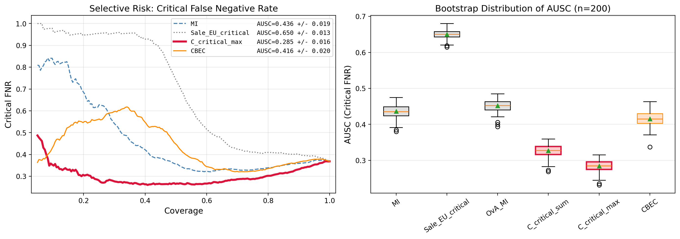
Uncertainty is estimated from \(S = 30\) stochastic forward passes through the posterior. Our primary safety metric is the critical false negative rate (Critical FNR, Appendix 9.8): among critical-class samples retained at a given coverage level, the fraction misclassified as safe. We summarise performance across coverage levels via the area under the selective risk curve (AUSC) [26], with 95% CIs from 200 bootstrap resamples. On the test set, the Bayesian model achieves accuracy \(0.8\) and quadratic weighted kappa \(0.65\); per-class performance in Appendix 10.3.
3.2 Deferral Policies↩︎
We compare 10 deferral policies across four families (Table ¿tbl:tab:policies?; formal definitions in Appendix 9).
4pt
lll Family & Policy & Score
& Entropy & \(H[\bar{p}]\)
& MI & \(H[\bar{p}] - \E[H[p^{(s)}]]\)
& MaxProb & \(1 - \max_k \mu_k\)
& Sale_EU_global & \(\sum_k \sigma^2_k\)
& Var_crit & \(\max_{k \in \mathcal{C}} \sigma^2_k\)
& Sale_EU_crit & \(\sum_{k \in \mathcal{C}} \sigma^2_k\)
Per-class MI & OvA_MI & \(\sum_{k \in \mathcal{C}} \mathrm{MI}_k^{\text{bin}}\)
& \(C_{\text{crit\_sum}}\) & \(\sum_{k \in \mathcal{C}} C_k\)
& \(C_{\text{crit\_max}}\) & \(\max_{k \in \mathcal{C}} C_k\)
& CBEC & Eq. [eq:cbec]
Scalar baselines are class-agnostic; per-class variance targets critical classes via raw \(\sigma^2_k\) but is confounded by \(\mu_k\) (Lemma 2); OvA_MI computes binary MI per critical class. Our three proposed metrics build on \(\sum_k C_k \approx \mathcal{I}\) (Section 2.2): \(C_{\text{crit\_max}}\) gives the sharpest signal when \(C_k\) estimates are reliable (\(\rho_k < 0.3\)); \(C_{\text{crit\_sum}}\) is a smoother alternative; CBEC (Eq. 12 ) gates safe–critical pairs by empirical negative correlation for robustness when skewness degrades \(C_k\).
3.3 Results↩︎
3.3.0.1 Theory validation.
Before evaluating downstream performance, we verify the additive decomposition 8 : \(\sum_k C_k\) and exact MI achieve Pearson \(r = 0.988\) and Spearman \(r = 0.998\) across all \(7{,}948\) test samples (Figure 4), confirming the second-order approximation preserves epistemic uncertainty rankings. The skewness diagnostic (Section 2.5) shows \(C_k\) is reliable (\(\rho_k < 0.3\)) for \({>}94\%\) of safe-class samples and \(82\%\)/\(63\%\) of Grade 2/3 respectively. Because the cutoff is a practical tolerance rather than a universal constant, we also sweep thresholds \(\tau \in \{0.1,0.2,0.3,0.5\}\) in Appendix 10.4. Tightening the criterion to \(\tau=0.1\) lowers the reliable fraction for critical grades to roughly \(68\)–\(75\%\), while relaxing it to \(\tau=0.5\) raises it to \(93\)–\(97\%\). The qualitative pattern is stable across thresholds: safe classes remain highly reliable, whereas rare critical classes are the most sensitive to higher-order Taylor terms.
3.3.0.2 Main results.
Table ¿tbl:tab:selective-bnn? reports AUSC and Critical FNR at 80% coverage with bootstrap CIs. \(C_{\text{crit\_max}}\) achieves the lowest AUSC (\(0.285\)), reducing the area under the selective risk curve by 34.7% relative to MI (\(0.436\), \(p < 0.005\)) and by 56.2% relative to Sale_EU_crit (\(0.650\), \(p < 0.005\)). At the clinically relevant 80% coverage operating point, \(C_{\text{crit\_max}}\) achieves FNR \(0.302\), compared to \(0.339\) for MI and \(0.409\) for Sale_EU_crit. Figure 1 visualises these results: \(C_{\text{crit\_max}}\) dominates across the full coverage range (left), with non-overlapping bootstrap interquartile ranges against scalar baselines (right). The improvement over raw variance is especially striking. Sale_EU_crit and Var_crit (AUSC \(0.650\) and \(0.606\)) perform worse than entropy (\(0.604\)), confirming that boundary suppression (Lemma 2) severely confounds unnormalised variance for critical classes with \(\mu_k \approx 0.06\). The \(1/\mu_k\) normalisation in \(C_k\) corrects precisely this: Grade 3 has mean probability \(\sim\)0.06, giving entropy curvature \(\sim\)17, so even small variance there carries large information-theoretic weight. This normalisation benefit is robust to the choice of inference method: a deep ensemble [3] of five members yields \(C_{\text{crit\_max}}\) AUSC \(0.390\) vs.\(0.447\) for Sale_EU_crit (\(12.9\%\) reduction; Appendix 10.13).
llcc Family & Policy & AUSC (Critical FNR)\(\downarrow\) & Critical FNR @80%\(\downarrow\)
& Entropy & \(0.604 \pm 0.022\) & \(0.401 \pm 0.016\)
& MI & \(0.436 \pm 0.019\) & \(0.339 \pm 0.014\)
& MaxProb & \(0.639 \pm 0.022\) & \(0.439 \pm 0.017\)
& Sale_EU_global & \(0.457 \pm 0.018\) & \(0.341 \pm 0.015\)
& Var_crit & \(0.606 \pm 0.014\) & \(0.379 \pm 0.016\)
& Sale_EU_crit & \(0.650 \pm 0.013\) & \(0.409 \pm 0.016\)
Per-class MI & OvA_MI & \(0.452 \pm 0.017\) & \(0.367 \pm 0.015\)
& \(C_{\text{crit\_sum}}\) & \(0.327 \pm 0.017\) & \(0.321 \pm 0.014\)
& \(C_{\text{crit\_max}}\) & \(\mathbf{0.285 \pm 0.016}\) & \(\mathbf{0.302 \pm 0.013}\)
& CBEC & \(0.416 \pm 0.020\) & \(0.335 \pm 0.014\)
3.3.0.3 Interpretability: Error Signatures.
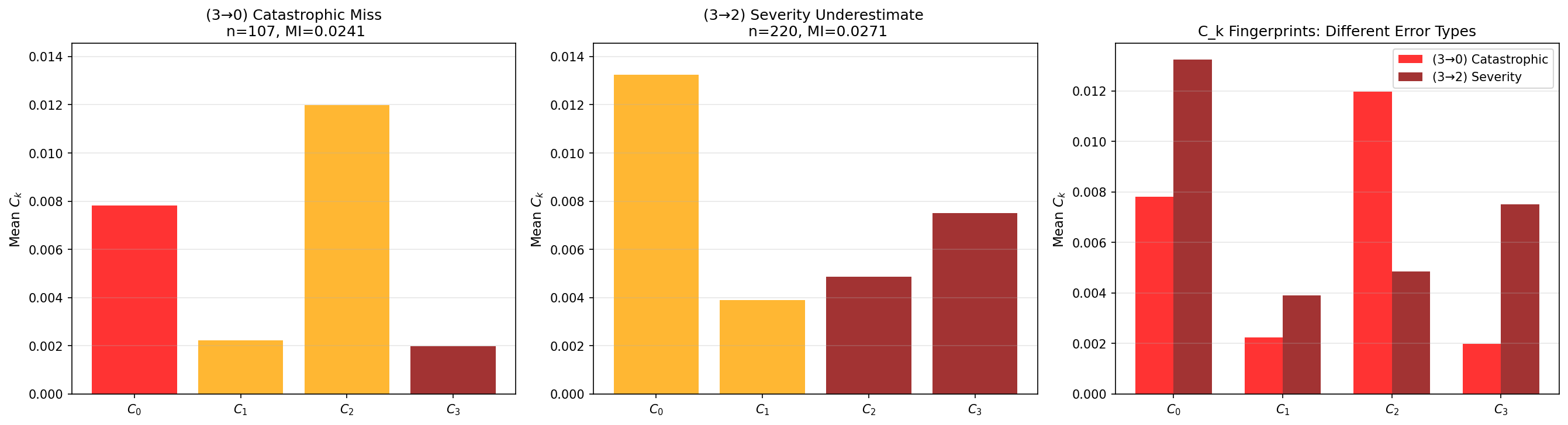
A distinctive advantage of \(\boldsymbol{C}(x)\) over scalar MI is that it reveals the structure of model confusion. Figure 2 shows that catastrophic misses (Grade 3 predicted as Grade 0) and severity underestimates (Grade 3 predicted as Grade 2) have nearly identical scalar MI (\(0.024\) vs.\(0.027\) nats) but very different \(C_k\) signatures. The catastrophic miss concentrates epistemic mass on \(C_2\), identifying Grade 2 as the bottleneck of confusion, while the severity underestimate elevates \(C_0\), indicating doubt about healthy status. These qualitatively different failure modes, invisible to scalar metrics, suggest distinct remediation strategies; the epistemic confusion matrix (Appendix 10.11) further confirms that cross-boundary confusion is \(2.7\times\) stronger than within-group confusion, validating the clinical partition (detailed analysis in Appendix 10.10).
3.3.0.4 Robustness across inference methods.
To test robustness to the posterior approximation, we repeat the evaluation using standard MC dropout [6] (\(p{=}0.3\), \(S{=}30\)). The ranking changes markedly: CBEC achieves the lowest AUSC (\(0.197 \pm 0.012\), winning 100% of bootstrap samples), a 53.6% reduction over MI (\(0.425 \pm 0.024\)), while \(C_{\text{crit\_max}}\) drops to \(0.419\). MC dropout is known to produce regions of spurious confidence where the approximate posterior underestimates uncertainty [14]. In our framework, this inflates \(\rho_k\) for critical classes, degrading the Taylor approximation underlying \(C_k\) while leaving CBEC’s correlation gate intact. A deep ensemble of five members confirms the pattern: CBEC again achieves the lowest AUSC (\(0.223\)), even though \(C_k\) reliability remains high (\(\rho_k < 0.3\) for \({>}85\%\) of Grade 3 samples), indicating that the correlation gate captures cross-boundary structure beyond what single-class targeting provides. This confirms the intended complementarity: \(C_{\text{crit\_max}}\) is the primary metric under well-calibrated posteriors; CBEC provides a robust alternative across inference regimes. Full results in Appendix 10.12 and 10.13.
4 Out-of-Distribution Detection↩︎
We evaluate the per-class epistemic uncertainty metric on out-of-distribution (OoD) detection, where elevated epistemic uncertainty is often used as a signal of distributional shift. This experiment should be read as a comparative within-posterior evaluation on the studied shifts, not as a claim that MI, \(\sum_k C_k\), \(EU_{\text{var}}\), or related uncertainty scores are universally reliable OoD detectors. In particular, uncertainty-based OoD scores can suffer from overconfidence failure modes in ReLU classifiers [27]; our question is whether, given the same predictive posterior, the class-resolved decomposition provides more useful separation and diagnostics than scalar alternatives.
4.1 Setup↩︎
4.1.0.1 Datasets.
We consider two OoD detection tasks: (1) FashionMNIST [28]\(\to\)KMNIST [29], a 10-class image task (50k/10k train/test, 10k OoD); and (2) MIMIC-III ICU [30]\(\to\)Newborn, binary mortality prediction on 44 tabular features (40k/4.5k train/test, 5.4k OoD).
4.1.0.2 Model.
Both tasks use low-rank Bayesian neural networks with Gaussian posteriors. FashionMNIST: two hidden layers (1200 units, rank 25), \(S{=}50\) MC samples. MIMIC-III: two hidden layers (128 units, rank 15), \(S{=}512\) MC samples, with class-weighted training to address mortality imbalance (8.6% prevalence). See Appendix 11.2 for full architectural and training details.
4.1.0.3 Metrics.
We compare four uncertainty scores: negative maximum softmax probability [31], MI, \(EU_{\text{var}} = \sum_k \sigma^2_k\), and our proposed \(\sum_k C_k\). Performance is measured by AUROC(ID samples labelled 0, OoD samples labelled 1); results are mean \(\pm\) std over 5 seeds.
4.2 Results↩︎
Table 1 summarises OoD detection performance. \(\sum_k C_k\) achieves the highest AUROC on both datasets: \(0.735\) on FashionMNIST versus \(0.724\) for MI, and \(0.815\) on MIMIC-III versus \(0.802\) for MI. The OoD-to-ID ratio column reveals the mechanism: on FashionMNIST, \(\sum_k C_k\) amplifies the distributional shift signal to \(6.43\times\) versus \(5.92\times\) for MI. On FashionMNIST, this effect is predicted by Lemma 4: the gap \(\sum_k C_k - \text{MI} \approx \frac{1}{6}\sum_k m_{3,k}/\mu_k^2\) grows with posterior skewness, and OoD samples produce higher skewness diagnostic \(\rho_k\) than ID samples across all ten classes (Appendix 11.6, Figure 14). On MIMIC-III the picture is more nuanced: the survival class (\(k{=}0\)) follows the expected pattern (\(\rho_0^{\text{OOD}} > \rho_0^{\text{ID}}\), median shift \(+43\%\)), but the mortality class (\(k{=}1\)) reverses because near-zero \(\mu_1\) for newborns collapses \(\mathrm{Var}[p_1]\) faster than \(1/\mu_1\) can compensate, concentrating the third-order signal entirely in class 0 (Appendix 11.6).
The unnormalised baseline \(EU_{\text{var}}\) underperforms MI on both datasets despite matching its ratio on FashionMNIST (\(5.92\times\)): without mean-normalisation, raw variance \(\sigma^2_k\) is bounded above by \(\mu_k(1-\mu_k)\), compressing the dynamic range of uncertainty scores. On MIMIC-III \(EU_{\text{var}}\) achieves the highest ratio (\(1.71\times\)) yet the lowest AUROC among epistemic measures. A high mean ratio does not imply good separability: AUROC depends on the full distributional overlap, and the un-normalised variance sum concentrates both ID and OoD scores near zero with a shared heavy tail, so the numerically large mean shift is swamped by within-group spread (Appendix 11.5, Figure 12). This pattern is consistent across inference methods: a deep ensemble replicates the same ranking (\(\sum_k C_k{=}0.753 > \text{MI}{=}0.752 > EU_{\text{var}}{=}0.750\)) on MIMIC-III, with \(EU_{\text{var}}\) again achieving the highest ratio (\(2.72\times\)) and the lowest AUROC (Appendix 11.7).
| FashionMNIST \(\to\) KMNIST | MIMIC-III ICU \(\to\) Newborn | ||||
|---|---|---|---|---|---|
| 3-4 (lr)5-6 Family | Method | AUROC\(\uparrow\) | Ratio\(\uparrow\) | AUROC\(\uparrow\) | Ratio\(\uparrow\) |
| Baselines | Neg.MSP | \(0.665 \pm 0.013\) | \(2.07\) | \(0.688 \pm 0.030\) | \(1.24\) |
| MI | \(0.724 \pm 0.009\) | \(5.92\) | \(0.802 \pm 0.004\) | \(1.61\) | |
| \(EU_{\text{var}}\) | \(0.710 \pm 0.010\) | \(5.92\) | \(0.778 \pm 0.015\) | \(\mathbf{1.71}\) | |
| Proposed | \(\sum_k C_k\) | \(\mathbf{0.735 \pm 0.009}\) | \(\mathbf{6.43}\) | \(\mathbf{0.815 \pm 0.017}\) | \(1.62\) |
4.2.0.1 Per-class decomposition.
On the binary MIMIC-III task, the decomposition \(\sum_k C_k = C_0 + C_1\) reveals that distributional shift affects the two classes asymmetrically (\(2.15\times\) for survival vs.\(1.30\times\) for mortality): the larger OoD signal resides in the non-critical class, so \(C_1\)-only yields AUROC \(0.740\), well below \(\sum_k C_k\) at \(0.815\). On FashionMNIST the pattern is broader but still uneven: all ten per-class \(C_k\) values increase from ID to OoD, but with substantially different magnitudes across classes (Appendix 11.4, Figure 11). Individual \(C_k\) scores yield non-trivial per-class OoD separation, but remain below the aggregate \(\sum_k C_k\), indicating that KMNIST induces a broad structural shift whose strength is distributed unevenly across the FashionMNIST label space. Together, these two cases illustrate a task-dependent trade-off: critical-class targeting improves selective prediction (Section 3) but all-class aggregation is necessary for OoD detection, where the locus of distributional shift is not known a priori and can be either asymmetric (MIMIC-III) or uniform (FashionMNIST).
Table 2 reports the corresponding per-class OoD scores for FashionMNIST\(\to\)KMNIST. Each individual \(C_k\) gives non-trivial ID/OoD separation, with AUROC ranging from \(0.537\) for Ankle boot to \(0.683\) for Bag. The ranking broadly tracks the OoD/ID amplification: classes with the largest increases, such as Bag, Trouser, and Sandal, also yield among the strongest per-class detectors. At the same time, all individual \(C_k\) scores remain below the aggregate \(\sum_k C_k\) AUROC of \(0.735 \pm 0.009\), confirming that this benchmark induces a broad shift for which aggregation is optimal, while the per-class decomposition reveals where the shift is strongest.
| Class | OoD/ID ratio | AUROC using \(C_k\) |
|---|---|---|
| T-shirt/top | \(6.971 \pm 0.788\) | \(0.670 \pm 0.027\) |
| Trouser | \(16.046 \pm 2.370\) | \(0.656 \pm 0.024\) |
| Pullover | \(3.477 \pm 0.549\) | \(0.578 \pm 0.020\) |
| Dress | \(9.428 \pm 1.005\) | \(0.662 \pm 0.020\) |
| Coat | \(3.481 \pm 0.602\) | \(0.577 \pm 0.026\) |
| Sandal | \(14.729 \pm 3.755\) | \(0.650 \pm 0.019\) |
| Shirt | \(4.467 \pm 0.337\) | \(0.615 \pm 0.025\) |
| Sneaker | \(3.494 \pm 0.906\) | \(0.549 \pm 0.054\) |
| Bag | \(18.854 \pm 2.173\) | \(0.683 \pm 0.030\) |
| Ankle boot | \(2.921 \pm 1.439\) | \(0.537 \pm 0.050\) |
5 Epistemic Sensitivity to Data Quality↩︎
We assess whether \(\sum_k C_k\) remains insensitive to irreducible aleatoric noise under controlled label-noise injection.
5.1 Setup↩︎
5.1.0.1 Data.
We use Fashion-MNIST (\(K{=}10\), 60,000 images) and CIFAR-10 (\(K{=}10\), 50,000 images) [32]. For each dataset we inject symmetric label noise at rates \(\alpha \in \{0.1, 0.2, 0.3, 0.4, 0.5\}\): a fraction \(\alpha\) of training labels is replaced uniformly at random, increasing aleatoric uncertainty without altering the input distribution.
5.1.0.2 Model.
We compare end-to-end Bayesian training with transfer learning using low-rank Gaussian posteriors (\(S{=}50\) MC samples). Fashion-MNIST: fully Bayesian; two hidden layers (\(400\) units, rank \(15\)). CIFAR-10: (i) end-to-end Conv \(32{\to}64{\to}128\), rank \(32\); (ii) frozen ResNet-18 with Bayesian head. Full details, alternative posteriors, and CIFAR-100 results in Appendix 12.1.
5.1.0.3 Protocol.
For each noise level \(\alpha\) we compute the mean aleatoric uncertainty \(\bar{U}_a(\alpha) = \frac{1}{N}\sum_i \mathbb{E}[H(\boldsymbol{p}_i)]\) and the mean epistemic uncertainty \(\bar{U}_e(\alpha)\) using either MI or \(\sum_k C_k\) over the clean test set. The relative disentanglement ratio \[\label{eq:disentangle-ratio} R_{\mathrm{rel}}(\alpha) \;=\; \frac{(\bar{U}_e(\alpha) - \bar{U}_e(0))\,/\,\bar{U}_e(0)}{(\bar{U}_a(\alpha) - \bar{U}_a(0))\,/\,\bar{U}_a(0)}\tag{13}\] measures the percentage increase in epistemic uncertainty per percentage increase in aleatoric uncertainty. \(R_{\mathrm{rel}} = 0\) indicates perfect disentanglement; \(R_{\mathrm{rel}} = 1\) indicates full entanglement; values above \(0.3\) signal substantial contamination (see Appendix 12.2 for the motivation behind the relative formulation over the absolute ratio).
5.2 Results↩︎
Table 3 reports \(|R_{\mathrm{rel}}|\) for low-rank Bayesian models under three configurations. Under end-to-end training, both metrics are near-perfectly disentangled (\(|R_{\mathrm{rel}}| \ll 0.3\) everywhere), confirming that end-to-end Bayesian training with low-rank posteriors is the regime that produces the least entangled uncertainty estimates. It is also the regime under which the second-order Taylor expansion most accurately approximates exact MI: at \(\alpha{=}0\), \(\sum_k C_k\,/\,\text{MI}\) is \(1.00\times\) on Fashion-MNIST and \(1.02\times\) on CIFAR-10 (Table 22). \(\sum_k C_k\) achieves lower \(|R_{\mathrm{rel}}|\) in 9 of the 10 end-to-end conditions, the exception being CIFAR-10 at \(\alpha{=}0.1\) where both values remain below \(0.05\). The rightmost block contrasts the same model type and dataset (CIFAR-10, low-rank) under transfer learning: ratios jump to \(0.74\)–\(1.97\), an order-of-magnitude degradation that isolates the training regime as the causal factor.
| FMNIST (e2e) | CIFAR-10 (e2e) | CIFAR-10 (TL) | ||||
|---|---|---|---|---|---|---|
| 2-3 (lr)4-5 (lr)6-7 \(\alpha\) | MI | \(\sum_k \Ck\) | MI | \(\sum_k \Ck\) | MI | \(\sum_k \Ck\) |
| 0.1 | 0.023 | \(\mathbf{0.005}^{\dagger}\) | \(\mathbf{0.040}\) | 0.047 | \(\mathbf{1.830}\) | 1.970 |
| 0.2 | 0.010 | \(\mathbf{0.003}^{\dagger}\) | 0.012 | \(\mathbf{0.007}^{\dagger}\) | \(\mathbf{1.344}\) | 1.435 |
| 0.3 | 0.008 | \(\mathbf{0.002}^{\dagger}\) | 0.009 | \(\mathbf{0.004}^{\dagger}\) | \(\mathbf{0.991}\) | 1.039 |
| 0.4 | 0.005 | \(\mathbf{0.003}^{\dagger}\) | 0.020 | \(\mathbf{0.016}^{\dagger}\) | \(\mathbf{0.832}\) | 0.868 |
| 0.5 | 0.009 | \(\mathbf{0.002}^{\dagger}\) | 0.020 | \(\mathbf{0.017}^{\dagger}\) | \(\mathbf{0.737}\) | 0.760 |
5.2.0.1 The posterior approximation matters as much as the metric.
Table 3 identifies training regime as a key factor. Under end-to-end training, posterior expressiveness tracks entanglement: on Fashion-MNIST the low-rank model achieves a mean \(|R_{\mathrm{rel}}|\) below \(0.01\) for both metrics, while the full-rank model reaches \(0.11\) (MI) / \(0.10\) (\(\sum_k C_k\)) and MC dropout \(0.10\) / \(0.06\) respectively (Appendix 12.2). Transfer learning disrupts this hierarchy: even the low-rank model produces \(|R_{\mathrm{rel}}|\) exceeding \(0.73\) on CIFAR-10, an order of magnitude worse than any end-to-end configuration, because the frozen backbone supplies features never optimised for calibrated predictive variance. This suggests that the high entanglement reported by [15] reflects the training regime as much as the decomposition formula. When uncertainty is not propagated through the full network, none of the three posterior families we evaluate can compensate, motivating the skewness diagnostic of Section 2.5 to flag such configurations. Across end-to-end settings (Figure 15), \(\sum_k C_k\) achieves lower \(|R_{\mathrm{rel}}|\) than MI in 19 of 20 conditions. Under transfer learning both metrics degrade and MI edges ahead, coinciding with baseline ratios \(\sum_k C_k\,/\,\text{MI}\) above roughly \(1.6\times\) (Table 22), i.e. where the Taylor residual is largest. Full transfer-learning results and an analysis of the rank constraint’s effect on uncertainty scale appear in Appendix 12.2.
5.2.0.2 Sensitivity to class cardinality.
On CIFAR-100 [32], the \(1/\mu_k\) normalisation amplifies contributions from low-probability classes, inflating \(\sum_k C_k\) relative to MI by \(1.17\times\) for the low-rank model and \(1.89\times\) for MC dropout. The \(\mathcal{O}(K^2)\) scaling analysis and mitigation strategies are detailed in Appendix 12.3.
6 Discussion and Conclusion↩︎
We presented a per-class epistemic uncertainty decomposition \(\boldsymbol{C}(x)\) derived from a second-order Taylor expansion of MI, where the \(1/\mu_k\) normalisation arises naturally from the entropy Hessian and counteracts boundary suppression. The decomposition reduces to a simple ratio of variance to mean per class, adds negligible cost to any posterior sampling pipeline, and closely tracks scalar MI by summation.
The three experiments exposed a consistent theme: the value of \(\boldsymbol{C}(x)\) lies not in being a better scalar summary but in enabling class-specific queries that scalar metrics cannot express. For selective prediction, targeting critical-class \(C_k\) outperformed all scalar and variance-based baselines; for OoD detection, the per-class view revealed that distributional shift can concentrate asymmetrically across classes, a structure invisible to any aggregate score; for disentanglement, the decomposition provided a lens to diagnose when and why epistemic and aleatoric signals become entangled.
A finding we did not anticipate is that the posterior approximation shaped metric behaviour at least as strongly as the metric itself. Switching from variational inference to MC dropout reversed the ranking of our deferral policies, because dropout inflated skewness precisely for the rare classes where the Taylor expansion is most sensitive. The disentanglement experiments sharpened this further: freezing a pretrained backbone and attaching a Bayesian head degraded AU/EU separation by over an order of magnitude compared to end-to-end training, even when the Bayesian component was identical. This raises a question for the growing literature on post-hoc Bayesian methods: if features are learned without any posterior objective, the resulting variance structure may not support meaningful epistemic attribution regardless of the last-layer treatment. We do not suggest post-hoc methods lack practical value, but the quality of their uncertainty outputs deserves scrutiny commensurate with the attention given to their scalability.
We note several limitations. The additive link \(\sum_k C_k\approx \mathcal{I}\) loosens under high skewness over low-probability classes, since the third-order remainder scales as \(1/\mu_k^2\); \(\rho_k\) diagnoses but does not correct this, and the CBEC fallback requires domain knowledge to define class partitions. The \(1/\mu_k\) normalisation introduces \(\mathcal{O}(K^2)\) scaling of the aggregate, necessitating truncation or reweighting in high-cardinality settings, though the per-class vector itself remains fully interpretable. Our CIFAR-100 experiments probe this cardinality effect in the disentanglement setting, but we do not evaluate high-cardinality OoD detection; ImageNet- or iNaturalist-scale class-conditional shifts remain an important stress test for future work.
All models use MFVI, low-rank Gaussian VI, MC dropout, or deep ensembles. Characterising how \(C_k\) behaves under other approximate inference schemes such as Laplace approximations [33] or stochastic weight averaging [34] is a natural next step.
The decomposition is not tied to any specific posterior family or architecture. Future work includes extending \(\boldsymbol{C}(x)\) to structured prediction tasks where class identity is less cleanly defined, integrating it into active learning acquisition functions that target specific classes, and combining low-rank ensembles with per-class attribution for richer uncertainty profiles. More fundamentally, making end-to-end Bayesian training more practical and scalable strikes us as a more promising path than refining post-hoc corrections, and the per-class decomposition is designed to complement that direction.4
7 Background and Related Work↩︎
This appendix provides the detailed literature context that supports the compressed survey in the main text. We organise the discussion into four parts: (i) the axiomatic framework and the label-wise variance approach; (ii) evidential and Dirichlet-based per-class uncertainty; (iii) class-imbalance and multi-class segmentation perspectives; and (iv) AU/EU disentanglement, scalar epistemic baselines, and the orthogonality criterion.
7.1 Axiomatic Framework and the Label-Wise Approach↩︎
7.1.0.1 Wimmer et al.(2023) – Axioms for epistemic uncertainty.
[8] formalise a set of axioms A0–A5 for second-order uncertainty measures in \(K\)-class classification. An uncertainty measure is defined over a second-order distribution \(Q \in \Delta^{(2)}_K\), a distribution over probability simplices \(\boldsymbol{p}\in \Delta^K\), with mean \(\boldsymbol{\mu}= \mathbb{E}_Q[\boldsymbol{p}]\). The five axioms relevant to our analysis are:
A0 (Non-negativity): \(\mathrm{EU}(Q) \geq 0\).
A1 (Vanishing at certainty): \(\mathrm{EU}(Q) = 0\) if and only if \(Q = \delta_{\boldsymbol{\theta}}\) for some \(\boldsymbol{\theta} \in \Delta^K\).
A2 (Maximum at uniform): \(\mathrm{EU}\) is maximised when \(Q\) is the uniform distribution on \(\Delta^K\).
A3 (Monotone under mean-preserving spread): if \(Q'\) is a mean-preserving spread of \(Q\) (i.e.\(Q'\) has the same mean but weakly larger variance in every direction), then \(\mathrm{EU}(Q') \geq \mathrm{EU}(Q)\).
A5 (Location-shift invariance): a spread-preserving shift of \(Q\)’s mean along the simplex does not change \(\mathrm{EU}(Q)\).
Wimmer et al.show that mutual information satisfies A0 and A1, but violates A2 (their Proposition 2), A3 (Proposition 4; a counterexample exists already for \(K{=}2\)), and A5 (Proposition 3). No single measure simultaneously satisfies all five axioms. Our aggregate \(\sum_k C_k\) satisfies A0, A1, and A3 but violates A2 and A5; as Corollary 1 establishes, the A5 violation is the precise mechanism that corrects boundary suppression.
7.1.0.2 Sale et al.(2024) – Label-wise decomposition.
[7] introduce a label-wise framework that reduces a \(K\)-class problem to \(K\) binary sub-problems via one-vs-rest binarisation. For each class \(k\), the true class probability \(\Theta_k\) is treated as a scalar random variable following a second-order distribution \(Q_k\) (capturing model uncertainty over possible probability values for class \(k\)). Per-class total, aleatoric, and epistemic uncertainty are defined via proper scoring rules; under squared loss the epistemic measure is \[\mathrm{EU}_k \;=\; \mathrm{Var}(\Theta_k),\] and the global quantities are sums: \(\mathrm{EU} = \sum_k \mathrm{Var}(\Theta_k)\). Sale et al.prove (their Theorem 3.2) that these variance-based measures satisfy axioms A0, A1, A3 (strict version), A4 (strict version), A5, A6, and A7, a stronger axiomatic profile than entropy-based measures, which fail A5 [8].
Two limitations motivate our normalised alternative. First, boundary suppression: because \(p_k \in [0,1]\), the constraint \(\mathrm{Var}[p_k] \leq \mu_k(1-\mu_k)\) (Lemma 2) forces \(\mathrm{EU}_k \to 0\) as \(\mu_k \to 0\), regardless of how strongly the stochastic forward passes disagree. This “edge-squeeze” masks epistemic uncertainty for precisely the rare, low-base-rate classes where it matters most, rendering \(\mathrm{EU}_k\) incomparable across classes with different mean probabilities. Second, the framework operates on marginals \(Q_k\) in isolation; consequently, the global sum \(\sum_k H(\bar{\theta}_k)\) does not recover the standard multiclass mutual information decomposition, preventing direct additive attribution of MI to individual classes. Our \(C_k\) addresses both limitations: the \(1/\mu_k\) normalisation removes the base-rate confound, and by construction \(\sum_k C_k \approx \mathcal{I}\) (Section 2.2).
7.2 Evidential and Dirichlet-Based Per-Class Uncertainty↩︎
7.2.0.1 Sensoy et al.(2018) and Malinin & Gales (2018).
[9] propose Evidential Deep Learning (EDL), training a neural network to output Dirichlet concentration parameters \(\boldsymbol{\alpha} = (\alpha_1,\dots,\alpha_K)\) in a single forward pass, thereby placing a distribution directly over the simplex. [10] independently introduced Prior Networks with the same Dirichlet parameterisation but a different training objective (reverse KL from a target Dirichlet), and formalised the decomposition of predictive uncertainty into distributional uncertainty (epistemic) and data uncertainty (aleatoric) within this framework. Both approaches provide per-class quantities derived from the Dirichlet parameters without requiring multiple stochastic forward passes.
7.2.0.2 Duan et al.(2024).
[11] extend the evidential paradigm by applying the law of total covariance to the Dirichlet-Categorical hierarchy. For a Dirichlet with concentration \(\boldsymbol{\alpha}\) and strength \(\alpha_0 = \sum_k \alpha_k\), they derive the full per-class epistemic covariance matrix (their Equation 21) \[\mathrm{Cov}^{\mathrm{epis}}_{c,c'} \;=\; \frac{1}{\alpha_0+1} \bigl(\bar{\mu}_c \,\mathbf{1}_{c=c'} - \bar{\mu}_c\bar{\mu}_{c'}\bigr),\] whose diagonal gives the per-class epistemic variance (Equation 24) \(U_c^{\mathrm{epis}} = \frac{1}{\alpha_0+1}\bar{\mu}_c(1-\bar{\mu}_c)\), and whose off-diagonal entries reveal pairwise class confusion. The covariance structure therefore carries both marginal and joint epistemic information in closed form.
However, the entire covariance matrix is determined solely by \(\bar{\boldsymbol{\mu}} = \boldsymbol{\alpha}/\alpha_0\) and the scalar strength \(\alpha_0\). This means that two inputs with the same Dirichlet mean but very different patterns of stochastic-forward-pass disagreement will receive identical epistemic covariance matrices, a rigidity absent from empirical MC-based estimates. More fundamentally, placing a Dirichlet prior on the simplex is a strong distributional assumption: the Dirichlet family is conjugate and analytically convenient, but real posterior predictive distributions under deep networks are rarely Dirichlet-shaped. Our approach makes no distributional assumption and recovers class-confusion information from the empirical covariance \(\widehat{\mathrm{Cov}}[\boldsymbol{p}]\) computed directly from MC samples.
7.3 Class Imbalance and Multi-Class Segmentation↩︎
7.3.0.1 Khan et al.(2019).
[13] demonstrate that MC-dropout predictive uncertainty (computed as the second moment of the softmax output across dropout masks, following [6]) correlates with both the rarity of classes and the difficulty of individual samples. They exploit this correlation to reshape classification margins: rare, high-uncertainty classes receive larger margin penalties, improving generalisation for under-represented classes across face verification, attribute prediction, and classification tasks. Importantly, the uncertainty used is the total predictive uncertainty (the combined effect of aleatoric and epistemic sources via the MC-dropout second moment); no explicit AU/EU decomposition is performed, and the uncertainty is used as a class-level signal derived from the training set rather than an input-level epistemic vector.
7.3.0.2 Baltaci et al.(2023).
[12] propose Class Uncertainty (CU), defined as the average predictive entropy across training examples within each class: \[\tilde{\mu}^U_c \;=\; \frac{1}{N_c}\sum_{i=1}^{N_c} u^{(i)}, \qquad u^{(i)} = -\sum_{c' \in \mathcal{C}} \bar{p}_{c'}^{(i)} \log \bar{p}_{c'}^{(i)},\] where \(\bar{p}_{c'}^{(i)}\) is the ensemble-averaged class probability for sample \(i\) (their Equations 8–9); a normalised version \(\mu^U_c = \tilde{\mu}^U_c / \sum_{c'} \tilde{\mu}^U_{c'}\) is then used as the class-imbalance weight (Equation 10). CU captures semantic imbalance, difficulty differences among classes that go beyond mere class cardinality, and is shown to correlate more strongly with class-wise test error than cardinality alone (Spearman \(\rho = 0.92\) vs.\(0.82\)).
CU has two limitations relative to our goal. First, it is a dataset-level aggregate: it aggregates over training examples and is not defined for a single test input, so it cannot provide input-level epistemic attribution. Second, it uses predictive entropy, which conflates aleatoric and epistemic components; no decomposition into EU and AU is performed.
7.3.0.3 Camarasa et al.(2021).
[35] provide a systematic quantitative comparison of epistemic uncertainty metrics in multi-class carotid artery MR segmentation, evaluating one-vs-all entropy, mutual information, and class-wise variance maps across both combined and class-specific settings. Their key empirical finding is that raw class-wise variance underperforms one-vs-all entropy in the class-specific setting (where it decorrelates from misclassification rate), while entropy-based metrics maintain stronger correlation with segmentation errors across all classes. Lemma 2 establishes this as a mathematical inevitability rather than a dataset artefact: variance is structurally suppressed near the simplex boundary regardless of actual posterior disagreement, making it an unreliable epistemic signal precisely where the information would be most valuable.
7.4 AU/EU Disentanglement, Scalar Baselines, and the Orthogonality Criterion↩︎
7.4.0.1 Smith & Gal (2018) – Taylor connection and MC-dropout failure modes.
[14] analyse the relationship between softmax variance and mutual information through a Taylor expansion of the logarithm. They show (their Equation 10, Section 3.2) that the leading term in the MI series is exactly proportional to the mean variance across classes: \[\hat{I} \;=\; \sum_j \!\left(\tfrac{1}{T}\textstyle\sum_i p_{ij}^2\right) - \hat{p}_j^2 + \mathcal{O}(\text{higher order}),\] which is, up to a multiplicative constant, the mean variance score \(\hat{\sigma}^2 = \frac{1}{C}\sum_j \mathrm{Var}[p_j]\). This provides a theoretical explanation for why variance-based uncertainty estimates empirically approximate MI and underscores the Taylor-expansion approach underlying our \(C_k\) decomposition; the key difference is that our expansion is applied per class rather than averaged, yielding class-level attribution.
Smith & Gal also document failure modes of MC-dropout: the approximate posterior tends to underestimate uncertainty and can produce spuriously confident regions in latent space where the model assigns high confidence to inputs far from any training data. We observe this behaviour in the DR experiment (Section 3): under MC-dropout, the skewness diagnostic \(\rho_k\) is elevated for critical (rare) classes, degrading the \(C_k\) Taylor approximation and causing \(C_{\mathrm{crit\_max}}\) to underperform its BNN counterpart.
7.4.0.2 Houlsby et al.(2011) – BALD and scalar epistemic uncertainty.
[5] introduce Bayesian Active Learning by Disagreement (BALD), originally for Gaussian processes and binary classifiers, selecting data points that maximise the mutual information \(\mathcal{I}(y;\boldsymbol{\omega}\mid x)\) between labels and model parameters; this objective was subsequently adopted as the canonical scalar epistemic measure in Bayesian deep learning [36]. BALD demonstrated its power for reducing posterior uncertainty in active learning. However, MI is class-agnostic: a high MI value signals that some class confusion is driving uncertainty, but does not identify which classes are the locus of the model’s ignorance. Our \(C_k\) vector decomposes MI into per-class contributions, preserving the additive structure of the BALD objective while exposing the class-level anatomy of epistemic uncertainty.
7.4.0.3 Hendrycks & Gimpel (2017) – Maximum softmax probability.
[31] demonstrate that the maximum softmax probability (MSP), \(\max_k \mu_k\), provides a surprisingly effective baseline for detecting both misclassified and out-of-distribution examples, despite the fact that softmax probabilities are known to be poorly calibrated as direct confidence estimates in deep networks. We include the complementary uncertainty score \(1 - \mathrm{MSP} = 1 - \max_k \mu_k\) as a scalar baseline in our deferral policy comparison (Table ¿tbl:tab:policies?). This score is agnostic to the source of uncertainty (aleatoric vs. epistemic) and to class identity, making it the most basic comparator against which our class-structured epistemic metrics are evaluated.
7.4.0.4 Mucsányi et al.(2024) – Benchmarking disentanglement.
[15] conduct a large-scale benchmark of uncertainty quantification methods and find that the aleatoric and epistemic components produced by standard decomposition formulas are highly rank-correlated across distributional methods: \(\rho(u_a, u_e) \geq 0.88\) on CIFAR-10 and \(\rho(u_a, u_e) \geq 0.78\) on ImageNet-1k. They interpret this as evidence that current methods fail to disentangle AU from EU, a conclusion that [16] subsequently show requires qualification.
7.4.0.5 de Jong et al.(2026) – Orthogonality as the correct criterion.
[16] formalise what it means for AU and EU estimates to be disentangled. They define two requirements, consistency (each estimate correlates with its corresponding ground-truth uncertainty) and orthogonality (each estimate is insensitive to changes in the other ground-truth uncertainty), and prove that both are necessary and sufficient for disentanglement (their Theorems 3.1–3.3).
A central theoretical result (Theorem 3.2) is that on complex datasets where aleatoric noise and epistemic difficulty co-occur, a high correlation between the estimators \(u_a\) and \(u_e\) is a necessary consequence of estimator validity, not a sign of failure; [15]’s high-\(\rho\) finding is therefore consistent with well-calibrated models on correlated datasets. The correct diagnostic is orthogonality, formalised as their Uncertainty Disentanglement Error (UDE). Evaluating a range of methods across multiple datasets, de Jong et al. find that Deep Ensembles with Information-Theoretic (IT) disentanglement achieve the best UDE, but that no current method fully satisfies both consistency and orthogonality.
Critically for our work, [16] show that disentanglement behaviour is strongly modulated by whether the model is trained from scratch or fine-tuned from a pretrained backbone (their Section 5, Figure 7). For a Deep Ensemble ResNet-18 pretrained on ImageNet-1k and fine-tuned to CIFAR-10, the UDE is substantially higher than for the same architecture trained from scratch (\(0.545\) vs.\(0.332\)), primarily because \(|{\rho(u_e, U_a)}| = 0.985\) in the pretrained case, aleatoric and epistemic uncertainty are almost fully conflated, compared to \(|{\rho(u_e, U_a)}| = 0.312\) for the from-scratch model. This finding is directly relevant to our Section 5, where we observe the same qualitative pattern independently: the \(C_k\) Taylor approximation degrades considerably when a frozen pretrained backbone replaces end-to-end Bayesian training, and the AU/EU entanglement of MI and \(\sum_k C_k\) increases markedly in the transfer-learning regime.
7.4.0.6 Depeweg et al.(2018) – AU/EU decomposition via total variance.
[2] formalise the decomposition of predictive uncertainty into aleatoric and epistemic components for latent-variable models. Applying the law of total variance to the predictive distribution \(p(y \mid x)\) marginalised over the posterior \(p(\omega \mid \mathcal{D})\) yields: \[\underbrace{\mathrm{Var}[y \mid x]}_{\text{total}} \;=\; \underbrace{\mathbb{E}_\omega[\mathrm{Var}[y \mid x, \omega]]}_{\text{aleatoric}} + \underbrace{\mathrm{Var}_\omega[\mathbb{E}[y \mid x, \omega]]}_{\text{epistemic}}.\] This identity is the regression analogue of the information-theoretic decomposition MI \(= H(\boldsymbol{\mu}) - \mathbb{E}[H(\boldsymbol{p})]\) used in classification; it also underlies the label-wise variance measures of [7], which interpret \(\mathrm{Var}(\Theta_k)\) as the epistemic contribution from class \(k\) via the same total-variance decomposition applied marginally.
8 Proofs↩︎
8.1 Proof of Theorem 1 (MI Approximation)↩︎
Proof. Expand \(H(\boldsymbol{p}^{(s)})\) to second order around \(\boldsymbol{\mu}\): \[H(\boldsymbol{p}^{(s)}) \;\approx\; H(\boldsymbol{\mu}) + \nabla H(\boldsymbol{\mu})^\top(\boldsymbol{p}^{(s)}-\boldsymbol{\mu}) + \tfrac{1}{2}(\boldsymbol{p}^{(s)}-\boldsymbol{\mu})^\top \nabla^2H(\boldsymbol{\mu})\,(\boldsymbol{p}^{(s)}-\boldsymbol{\mu}).\] Take expectations over the \(S\) passes. The linear term vanishes by definition of \(\boldsymbol{\mu}= \mathbb{E}[\boldsymbol{p}^{(s)}]\). By Lemma 1 the Hessian is \(\nabla^2H(\boldsymbol{\mu})=\mathrm{diag}(-1/\mu_1,\dots,-1/\mu_K)\), so the quadratic term becomes \[\tfrac{1}{2}\,\mathbb{E}\!\left[ (\boldsymbol{p}-\boldsymbol{\mu})^\top\nabla^2H(\boldsymbol{\mu})\,(\boldsymbol{p}-\boldsymbol{\mu}) \right] = \tfrac{1}{2}\,\mathrm{tr}\!\left[ \nabla^2H(\boldsymbol{\mu})\,\mathrm{Cov}[\boldsymbol{p}] \right] = -\frac{1}{2}\sum_{k=1}^{K}\frac{\mathrm{Var}[p_k]}{\mu_k}.\] The second equality uses the fact that the Hessian is diagonal, so the trace selects only the diagonal elements of \(\mathrm{Cov}[\boldsymbol{p}]\): \(\mathrm{tr}[\mathrm{diag}(-1/\mu_k)\,\mathrm{Cov}[\boldsymbol{p}]]= -\sum_k\mathrm{Var}[p_k]/\mu_k\). Substituting into 3 gives \[\mathcal{I}(y;\boldsymbol{\omega}\mid x) = H(\boldsymbol{\mu})-\mathbb{E}[H(\boldsymbol{p})] \;\approx\; \frac{1}{2}\sum_{k=1}^{K}\frac{\mathrm{Var}[p_k](x)}{\mu_k(x)},\] with remainder \(O(\mathbb{E}[\|\boldsymbol{p}-\boldsymbol{\mu}\|^3])\) from the discarded cubic terms. ◻
8.1.0.1 Remark on the simplex constraint.
The constraint \(\sum_k p_k=1\) forces \(\sum_k(p_k-\mu_k)=0\), so \(\mathrm{Cov}[\boldsymbol{p}]\) has zero row- and column-sums and rank at most \(K-1\). This does not invalidate the trace formula: the approximation operates on the full \(K\)-dimensional covariance, and the simplex constraint is already absorbed into the empirical estimates 1 –2 . Summing 6 over all \(K\) classes therefore remains valid.
8.2 Proofs of Lemmas 2 and 3↩︎
Proof of Lemma 2 (Variance Bound on the Simplex). Since \(p_k^{(s)}\in[0,1]\) implies \((p_k^{(s)})^2\leq p_k^{(s)}\), we have \[\mathrm{Var}[p_k] = \mathbb{E}[p_k^2]-\mu_k^2 \leq \mathbb{E}[p_k]-\mu_k^2 = \mu_k - \mu_k^2 = \mu_k(1-\mu_k).\] Since \(\mu_k(1-\mu_k)\to 0\) as \(\mu_k\to 0\) or \(\mu_k\to 1\), we have \(\mathrm{Var}[p_k]\to 0\) at the simplex boundary regardless of the degree of disagreement among the \(S\) forward passes. ◻
Proof of Lemma 3 (Boundary Behaviour of \(C_k\)). Dividing both sides of 9 by \(2\mu_k>0\): \[C_k = \frac{1}{2}\,\frac{\mathrm{Var}[p_k]}{\mu_k} \;\leq\; \frac{1}{2}\,\frac{\mu_k(1-\mu_k)}{\mu_k} = \frac{1}{2}(1-\mu_k).\] As \(\mu_k\to 0\), the upper bound \(\tfrac{1}{2}(1-\mu_k)\to\tfrac{1}{2}\), so \(C_k\) is not forced to zero near the simplex boundary. ◻
8.2.0.1 Remark on attainability.
The variance bound is tight: it is attained when \(p_k^{(s)}\in\{0,1\}\) for all \(s\), i.e., each forward pass is maximally confident about class \(k\) but the passes disagree on the direction. In this case \(\mathrm{Var}[p_k]=\mu_k(1-\mu_k)\) and \(C_k=\tfrac{1}{2}(1-\mu_k)\approx\tfrac{1}{2}\) for \(\mu_k\ll 1\): exactly the non-vanishing signal that motivates the normalisation.
8.3 Proof of Theorem 2↩︎
We follow the axiomatic framework of [8], as extended by [7]. Throughout, \(Q \in \Delta^{(2)}_K\) is a second-order distribution over probability vectors \(\boldsymbol{p}\in \Delta^{K-1}\), with mean \(\boldsymbol{\mu}= \mathbb{E}_Q[\boldsymbol{p}]\). We write \(\mathrm{EU}(Q) = \sum_{k=1}^K C_k = \tfrac{1}{2}\sum_{k=1}^K \mathrm{Var}[p_k]/\mu_k\).
8.3.0.1 Axioms evaluated.
A0 (Non-negativity): \(\mathrm{EU}(Q) \geq 0\).
A1 (Vanishing at certainty): \(\mathrm{EU}(Q) = 0\) iff \(Q = \delta_{\boldsymbol{\theta}}\) for some \(\boldsymbol{\theta} \in \Delta^{K-1}\).
A2 (Maximality at uniform): \(\mathrm{EU}\) is maximised when \(Q = Q_{\mathrm{unif}}\), the uniform distribution on \(\Delta^{K-1}\).
A3 (Monotone under MPS, strict version): if \(Q'\) is a mean-preserving spread of \(Q\) then \(\mathrm{EU}(Q') > \mathrm{EU}(Q)\).
A5 (Location-shift invariance): if \(Q'\) is a spread-preserving location shift of \(Q\) then \(\mathrm{EU}(Q') = \mathrm{EU}(Q)\).
8.3.0.2 Definitions.
Following [7] (Definition 2.1), \(Q'\) is a mean-preserving spread (MPS) of \(Q\) if \(\boldsymbol{p}' \stackrel{d}{=} \boldsymbol{p}+ \boldsymbol{Z}\) where \(\boldsymbol{Z}\) satisfies \(\mathbb{E}[\boldsymbol{Z} \mid \sigma(\boldsymbol{p})] = \boldsymbol{0}\) a.s.and \(\max_k \mathrm{Var}[Z_k] > 0\). \(Q'\) is a spread-preserving location shift of \(Q\) if \(\boldsymbol{p}' \stackrel{d}{=} \boldsymbol{p}+ \boldsymbol{z}\) for some constant \(\boldsymbol{z} \neq \boldsymbol{0}\).
Proof. A0. \(\mathrm{Var}[p_k] = \mathbb{E}[p_k^2] - \mu_k^2 \geq 0\) by Jensen’s inequality. When \(\mu_k > 0\), \(C_k = \tfrac{1}{2}\mathrm{Var}[p_k]/\mu_k \geq 0\). When \(\mu_k = 0\): \(p_k \geq 0\) and \(\mathbb{E}[p_k] = 0\) imply \(p_k = 0\) \(Q\)-a.s., so \(\mathrm{Var}[p_k] = 0\) and \(C_k := 0\) by convention. Hence \(\mathrm{EU}(Q) = \sum_k C_k \geq 0\).
A1. (\(\Rightarrow\)) If \(Q = \delta_{\boldsymbol{\theta}}\), then \(\mathrm{Var}[p_k] = 0\) for every \(k\), so \(\mathrm{EU}(Q) = 0\). (\(\Leftarrow\)) Suppose \(\mathrm{EU}(Q) = 0\). Since each \(C_k \geq 0\) and \(\sum_k C_k = 0\), every \(C_k = 0\). For \(\mu_k > 0\) this forces \(\mathrm{Var}[p_k] = 0\), hence \(p_k = \mu_k\) \(Q\)-a.s. For \(\mu_k = 0\), \(p_k = 0 = \mu_k\) \(Q\)-a.s.by non-negativity of \(p_k\). Hence \(\boldsymbol{p}= \boldsymbol{\mu}\) \(Q\)-a.s., i.e.\(Q = \delta_{\boldsymbol{\mu}}\).
A3 (strict). Let \(\boldsymbol{p}' \stackrel{d}{=} \boldsymbol{p}+ \boldsymbol{Z}\) with \(\mathbb{E}[\boldsymbol{Z} \mid \sigma(\boldsymbol{p})] = \boldsymbol{0}\) a.s.and \(\max_k \mathrm{Var}[Z_k] > 0\).
Mean preservation. \(\mu_k' = \mathbb{E}[p_k + Z_k] = \mu_k + \mathbb{E}\!\bigl[\mathbb{E}[Z_k \mid \sigma(\boldsymbol{p})]\bigr] = \mu_k\).
Variance expansion. \[\begin{align} \mathrm{Var}[p_k'] = \mathrm{Var}[p_k + Z_k] = \mathrm{Var}[p_k] + \mathrm{Var}[Z_k] + 2\,\mathrm{Cov}[p_k, Z_k]. \end{align}\] The cross-term vanishes by the tower property and \(\sigma(\boldsymbol{p})\)-measurability of \(p_k\): \[\mathrm{Cov}[p_k, Z_k] = \mathbb{E}[p_k Z_k] - \mathbb{E}[p_k]\mathbb{E}[Z_k] = \mathbb{E}\!\Bigl[\mathbb{E}[p_k Z_k \mid \sigma(\boldsymbol{p})]\Bigr] - \mathbb{E}[p_k]\cdot\mathbb{E}\!\Bigl[\mathbb{E}[Z_k \mid \sigma(\boldsymbol{p})]\Bigr] = \mathbb{E}\!\Bigl[p_k\underbrace{\mathbb{E}[Z_k \mid \sigma(\boldsymbol{p})]}_{=\;0}\Bigr] - \mathbb{E}[p_k]\cdot 0 = 0.\] Hence \(\mathrm{Var}[p_k'] = \mathrm{Var}[p_k] + \mathrm{Var}[Z_k]\), and since \(\mu_k' = \mu_k\), we have \(C_k(Q') \geq C_k(Q)\) for all \(k\).
Strict increase. By the MPS condition, \(\mathrm{Var}[Z_j] > 0\) for some \(j\). We show \(\mu_j > 0\). If \(\mu_j = 0\) then \(p_j = 0\) \(Q\)-a.s., so \(p_j' = Z_j\). Since \(\boldsymbol{p}' \in \Delta^{K-1}\), we have \(p_j' \geq 0\), hence \(Z_j \geq 0\) \(Q\)-a.s. Combined with \(\mathbb{E}[Z_j] = \mathbb{E}\!\bigl[\mathbb{E}[Z_j \mid \sigma(\boldsymbol{p})]\bigr] = 0\), this forces \(Z_j = 0\) \(Q\)-a.s., contradicting \(\mathrm{Var}[Z_j] > 0\). Hence \(\mu_j > 0\), giving \(C_j(Q') = \tfrac{1}{2}(\mathrm{Var}[p_j]+\mathrm{Var}[Z_j])/\mu_j > C_j(Q)\), and therefore \(\mathrm{EU}(Q') > \mathrm{EU}(Q)\).
A2 violated. Lemma 2 gives \(\mathrm{Var}[p_k] \leq \mu_k(1-\mu_k)\), so \[\mathrm{EU}(Q) = \frac{1}{2}\sum_{k=1}^K\frac{\mathrm{Var}[p_k]}{\mu_k} \leq \frac{1}{2}\sum_{k=1}^K(1-\mu_k) = \frac{K-1}{2},\] using \(\sum_k \mu_k = 1\). The bound is attained by the uniform vertex mixture \(Q_{\mathrm{vert}} = \frac{1}{K}\sum_{y=1}^K \delta_{\mathbf{e}_y}\), for which \(\mu_k = 1/K\), \(\mathrm{Var}[p_k] = \mathbb{E}[p_k^2] - \mu_k^2 = 1/K - 1/K^2 = (K-1)/K^2\), and \(\mathrm{EU}(Q_{\mathrm{vert}}) = (K-1)/2\). By contrast, the uniform distribution on \(\Delta^{K-1}\) equals \(\mathrm{Dirichlet}(\mathbf{1}_K)\), whose marginals satisfy \(\mathrm{Var}[p_k] = (K-1)/[K^2(K+1)]\) (standard Dirichlet second moment), giving \[\mathrm{EU}(Q_{\mathrm{unif}}) = K \cdot \frac{1}{2} \cdot \frac{(K-1)/[K^2(K+1)]}{1/K} = \frac{K-1}{2(K+1)} < \frac{K-1}{2} = \mathrm{EU}(Q_{\mathrm{vert}}) \quad \forall\, K \geq 2.\] Hence \(Q_{\mathrm{unif}}\) is not the maximiser and A2 is violated.
A5 violated. Under \(\boldsymbol{p}' = \boldsymbol{p}+ \boldsymbol{z}\) (constant \(\boldsymbol{z}\)): \(\mathrm{Var}[p_k'] = \mathrm{Var}[p_k]\) by translation-invariance of variance, but \(\mu_k' = \mu_k + z_k\), so \(C_k(Q') = \tfrac{1}{2}\mathrm{Var}[p_k]/(\mu_k + z_k) \neq C_k(Q)\) whenever \(z_k \neq 0\) and \(\mathrm{Var}[p_k] > 0\). Concretely, let \(K = 2\) and \(Q = \tfrac{1}{2}\delta_{(0.2,\,0.8)} + \tfrac{1}{2}\delta_{(0.4,\,0.6)}\), so \(\boldsymbol{\mu}= (0.3,\,0.7)\), \(\mathrm{Var}[p_k] = 0.01\) for both \(k\), and \(\mathrm{EU}(Q) \approx 0.0238\). Under \(\boldsymbol{z} = (0.15,\,-0.15)\): \(\boldsymbol{\mu}' = (0.45,\,0.55)\), variances unchanged, giving \(\mathrm{EU}(Q') \approx 0.0202 \neq \mathrm{EU}(Q)\). ◻
Remark 4 ([8] Proposition 4). Exact MI violates the strict version of A3 already for \(K = 2\). The improvement of \(\sum_k C_k\) is a direct consequence of its linearity in \(\{\mathrm{Var}[p_k]\}\): any non-trivial spread in any class propagates immediately into a strict increase of the aggregate.
| Axiom | \(\sum_k \Ck\) (ours) | Exact MI | \(\Var(\Theta_k)\) |
|---|---|---|---|
| A0: Non-negativity | |||
| A1: Vanishing EU | |||
| A2: Maximality at uniform | |||
| A3: Monotonicity (MPS) | |||
| A5: Location-shift invariance |
9 Complete Metric Reference↩︎
This appendix collects, in self-contained form, the definitions and interpretations of every uncertainty metric evaluated in the selective prediction experiments. Throughout, we adopt the notation of Section 2: \(S\) stochastic forward passes produce probability vectors \(\boldsymbol{p}^{(s)}(x)\in\Delta^{K-1}\), \(s=1,\dots,S\), from which all subsequent quantities are estimated.
9.1 Monte Carlo Prediction Statistics↩︎
The following sample statistics, computed from the \(S\) stochastic forward passes, serve as building blocks for all metrics defined below.
9.1.0.1 Mean prediction.
The predictive mean \[\label{eq:app-mu} \mu_k \;=\; \frac{1}{S}\sum_{s=1}^{S} p_k^{(s)}, \qquad k = 0,\dots,K{-}1,\tag{14}\] represents the model’s consensus probability for class \(k\). The predicted label is \(\hat{y}=\arg\max_k \mu_k\).
9.1.0.2 Per-class variance and covariance.
The sample variance and covariance, with Bessel correction, are \[\begin{align} \sigma_k^2 &\;=\; \frac{1}{S-1}\sum_{s=1}^{S}\bigl(p_k^{(s)}-\mu_k\bigr)^2, \tag{15}\\[4pt] \Sigma_{ij} &\;=\; \frac{1}{S-1}\sum_{s=1}^{S} \bigl(p_i^{(s)}-\mu_i\bigr)\bigl(p_j^{(s)}-\mu_j\bigr), \tag{16} \end{align}\] with Pearson correlation \(\rho_{ij}=\Sigma_{ij}/(\sigma_i\,\sigma_j)\). A strongly negative \(\rho_{ij}\) indicates that probability mass flows systematically from class \(j\) to class \(i\) across forward passes, i.e.the model actively confuses the two classes.
9.1.0.3 Third central moment.
\[\label{eq:app-m3} m_{3,k} \;=\; \frac{1}{S}\sum_{s=1}^{S} \bigl(p_k^{(s)}-\mu_k\bigr)^3.\tag{17}\] This quantity enters only through the skewness diagnostic \(\rho_k\) defined in Section 9.7.
9.2 Scalar Uncertainty Baselines↩︎
The following standard metrics assign a single uncertainty score to each input and do not distinguish between classes.
9.2.0.1 Predictive entropy.
The Shannon entropy of the mean prediction, \[\label{eq:app-ent} H[\bar{p}] \;=\; -\sum_{k=0}^{K-1}\mu_k\log\mu_k,\tag{18}\] lies in \([0,\log K]\) and captures total predictive uncertainty, both epistemic and aleatoric. It cannot distinguish a model that lacks training data from one facing a genuinely ambiguous input; nor does it differentiate clinically benign confusions (e.g.Grade 0 vs.Grade 1) from dangerous ones (Grade 0 vs.Grade 3).
9.2.0.2 Mutual information.
\[\label{eq:app-mi} \mathrm{MI} \;=\; H[\bar{p}] \;-\; \frac{1}{S}\sum_{s=1}^{S}H\bigl[\boldsymbol{p}^{(s)}\bigr],\tag{19}\] where \(H[\boldsymbol{p}^{(s)}]=-\sum_k p_k^{(s)}\log p_k^{(s)}\). MI isolates epistemic uncertainty by subtracting the average per-pass entropy (the aleatoric component): if all \(S\) passes produce identical softmax vectors, MI vanishes regardless of how uncertain those vectors are. While MI is the standard scalar epistemic measure, it remains a single number that cannot reveal which classes drive the model’s disagreement. Two inputs with identical MI may involve entirely different confusion patterns, as demonstrated by the error signatures in Section 10.10.
9.2.0.3 Maximum softmax uncertainty.
\[\label{eq:app-maxprob} \mathrm{MaxProb} \;=\; 1 - \max_k\;\mu_k\,.\tag{20}\] This is the simplest deferral baseline: it uses only the mean prediction and does not exploit MC disagreement. MaxProb is insensitive to the distribution of probability across non-top classes; two inputs \(\mu=(0.6,\,0.4,\,0,\,0)\) and \(\mu=(0.6,\,0,\,0.4,\,0)\) receive identical scores despite the latter involving a dangerous safe–critical confusion.
9.3 Per-Class Variance Baselines↩︎
These metrics use the raw per-class variance \(\sigma_k^2\) as a proxy for epistemic disagreement, without the \(1/\mu_k\) normalisation that defines \(C_k\).
9.3.0.1 Critical variance.
\[\label{eq:app-varcrit} \mathrm{Var\_crit} \;=\; \max_{k\in\mathcal{C}}\;\sigma_k^2\,,\tag{21}\] where \(\mathcal{C}=\{2,3\}\) denotes the set of critical (treatment-requiring) classes. This provides a targeted measure of MC disagreement restricted to critical classes, but inherits the base-rate confound identified in Lemma 2: a class with \(\mu_k=0.5\) naturally exhibits higher variance than one with \(\mu_k=0.01\), even at equal levels of epistemic disagreement in logit space.
9.3.0.2 Global and critical variance baselines.
[7] explicitly define the global variance-based epistemic uncertainty measure (their equation 22): \[\mathrm{Sale\_EU\_global} \;=\; \sum_{k=0}^{K-1}\sigma_k^2\,, \label{eq:app-sale-global}\tag{22}\] which aggregates label-wise variance over all classes and constitutes a scalar epistemic measure directly comparable to MI and \(\sum_k C_k\). We additionally construct a critical-class restriction not defined by [7]: \[\mathrm{Sale\_EU\_crit} \;=\; \sum_{k\in\mathcal{C}}\sigma_k^2\,, \label{eq:app-sale-crit}\tag{23}\] which provides a targeted analogue of \(C_{\mathrm{crit\_sum}}\) without curvature normalisation. Both variants suffer from the same boundary suppression as \(\mathrm{Var\_crit}\): for critical classes with mean prediction \(\mu_k\approx 0.06\) in our data, variance is bounded by \(\mu_k(1-\mu_k)\approx 0.056\) regardless of the degree of model disagreement (cf.Section 2.3).
9.4 One-vs-All MI Baseline↩︎
An alternative per-class decomposition computes binary mutual information for each class independently. For class \(k\), define the binary variable \(q_k^{(s)}=(p_k^{(s)},\;1-p_k^{(s)})\) and the corresponding binary MI \[\label{eq:app-ova} \mathrm{MI}_k^{\mathrm{bin}} \;=\; H[\bar{q}_k] \;-\; \frac{1}{S}\sum_{s=1}^{S}H\bigl[q_k^{(s)}\bigr].\tag{24}\] The deferral score sums over critical classes: \(\mathrm{OvA\_MI}=\sum_{k\in\mathcal{C}}\mathrm{MI}_k^{\mathrm{bin}}\). This measure is exact (not Taylor-approximated) but discards the multi-class structure: it does not reveal which non-\(k\) classes compete with class \(k\), and the per-class binary MI terms are not additive components of the full multiclass MI.
9.5 Proposed Metrics: Per-Class Epistemic Decomposition↩︎
The metrics in this subsection are derived from the second-order Taylor expansion of mutual information developed in Section 2.
9.5.0.1 Per-class epistemic contribution.
The central quantity is the per-class component \[\label{eq:app-Ck} C_k \;=\; \frac{1}{2}\,\frac{\sigma_k^2}{\mu_k}\tag{25}\] which satisfies \(\sum_{k=0}^{K-1}C_k\approx\mathrm{MI}\) by Theorem 1. The \(1/\mu_k\) weighting originates from the curvature of the entropy surface (\(\partial^2 H/\partial p_k^2=-1/\mu_k\)): a class with \(\mu_k=0.01\) has curvature \(100\), so even modest probability variance there carries substantial information-theoretic weight, whereas a class with \(\mu_k=0.5\) requires proportionally larger variance to indicate genuine epistemic uncertainty. The ratio \(\sigma_k^2/\mu_k\) coincides with the classical index of dispersion [17], [18]; the \(\tfrac{1}{2}\) prefactor arises from the Hessian structure, ensuring that the components sum to MI rather than twice MI.
The approximation is reliable when the MC distribution for each class is approximately symmetric. Reliability is diagnosed by the skewness indicator \(\rho_k\) (Section 9.7): when \(\rho_k>0.3\) for a critical class, \(C_k\) should be interpreted with caution and CBEC (Section 9.6) is preferred.
9.5.0.2 Critical-class aggregations.
Two natural aggregations restrict attention to the critical class set \(\mathcal{C}\): \[\begin{align} C_{\mathrm{crit\_max}} &\;=\; \max_{k\in\mathcal{C}}\;C_k\,, \tag{26}\\[4pt] C_{\mathrm{crit\_sum}} &\;=\; \sum_{k\in\mathcal{C}}C_k\,. \tag{27} \end{align}\] \(C_{\mathrm{crit\_max}}\) is sensitive to single-class spikes: it fires when any critical class carries elevated epistemic uncertainty, and is the recommended aggregation when \(\rho_k<0.3\) for all critical classes. \(C_{\mathrm{crit\_sum}}\) is a smoother alternative that captures cumulative uncertainty when confusion is distributed across multiple critical classes.
9.6 Boundary-Aware Metrics↩︎
The metrics above score each class (or class subset) in isolation. In applications with a clinically meaningful partition into safe classes \(\mathcal{S}=\{0,1\}\) and critical classes \(\mathcal{C}=\{2,3\}\), the most dangerous errors are those that cross this boundary. The following metric targets such cross-boundary confusion directly.
9.6.0.1 Cross-boundary epistemic confusion (CBEC).
\[\label{eq:app-cbec} \mathrm{CBEC}(x) \;=\; \sum_{i\in\mathcal{S}}\;\sum_{j\in\mathcal{C}} \sqrt{C_i\cdot C_j}\;\cdot\;\max(0,\,-\rho_{ij}).\tag{28}\] CBEC is non-zero only when three conditions hold simultaneously: a safe class carries elevated \(C_i\), a critical class carries elevated \(C_j\), and their MC predictions are negatively correlated (\(\rho_{ij}<0\)), indicating that probability mass flows systematically from one to the other across stochastic passes. The geometric mean \(\sqrt{C_i C_j}\) requires both classes to be uncertain, and the correlation gate \(\max(0,-\rho_{ij})\) filters coincidental co-elevation.
CBEC is partially robust to degradation of the Taylor approximation for two reasons. First, the correlation \(\rho_{ij}\) is computed directly from MC samples and does not depend on the second-order expansion. Second, the geometric mean compresses outlier inflation: if skewness inflates \(C_j\) by a factor of \(\alpha\), the geometric mean is inflated by only \(\sqrt{\alpha}\). These properties explain CBEC’s empirical robustness under MC dropout, where \(C_k\) estimates for rare critical classes degrade (Section 10.12).
9.7 Diagnostic Metrics↩︎
The following quantities assess the reliability and structure of the \(C_k\) estimates. They are not used as deferral scores.
9.7.0.1 Skewness diagnostic.
For each class \(k\) with \(\sigma_k^2>0\), the ratio \[\label{eq:app-rho} \rho_k \;=\; \frac{|m_{3,k}|}{3\,\mu_k\cdot\sigma_k^2}\tag{29}\] equals the magnitude of the third-order Taylor correction relative to the second-order term \(C_k\) (see Section 2.5). When \(\rho_k\ll 1\), the cubic remainder is negligible and \(C_k\) is reliable; when \(\rho_k>0.3\), the second-order approximation is degrading and \(C_k\) should be supplemented or replaced by CBEC. In practice, majority classes (high \(\mu_k\), far from the simplex boundary) produce approximately symmetric MC distributions and low \(\rho_k\); rare classes (\(\mu_k\approx 0\)) produce right-skewed distributions bounded by zero and correspondingly higher \(\rho_k\).
9.7.0.2 Epistemic profiles.
For each true class \(i\), the normalised conditional expectation \[\label{eq:app-profile} \mathrm{Profile}_k(i) \;=\; \mathbb{E}\!\Bigl[\frac{C_k}{\textstyle\sum_j C_j} \;\Big|\; y=i\Bigr], \qquad k=0,\dots,K{-}1,\tag{30}\] reveals the average distribution of epistemic uncertainty across classes for inputs of true class \(i\). For example, a profile \((0.14,\,0.27,\,0.55,\,0.05)\) for Grade 0 images indicates that the model’s uncertainty about healthy images concentrates predominantly on Grade 2 (moderate DR), signalling systematic Grade 0–Grade 2 confusion.
9.7.0.3 Error epistemic signatures.
Conditioning on both true and predicted labels yields the error-type signature \[\label{eq:app-sig} \mathrm{Sig}_k(i\!\to\!j) \;=\; \mathbb{E}\bigl[C_k \;\big|\; y=i,\;\hat{y}=j\bigr], \qquad k=0,\dots,K{-}1.\tag{31}\] Different error types produce distinct \(C_k\) fingerprints even when their scalar MI is similar, enabling targeted diagnostic interpretation (see Section 10.10).
9.7.0.4 Epistemic confusion matrix.
\[\label{eq:app-eij} E_{ij} \;=\; \mathbb{E}\!\bigl[\sqrt{C_i\cdot C_j} \;\cdot\;\max(0,-\rho_{ij})\bigr].\tag{32}\] Entry \(E_{ij}\) quantifies the average directed epistemic confusion between classes \(i\) and \(j\), aggregated over the test set. The matrix is symmetric with zero diagonal (since \(\rho_{kk}=1\) implies \(\max(0,-\rho_{kk})=0\)). High values in the \(\mathcal{S}\times\mathcal{C}\) block indicate that the model’s epistemic uncertainty concentrates at the clinically dangerous boundary, validating both the safe–critical partition and the CBEC aggregation.
9.8 Evaluation Metrics for Selective Prediction↩︎
The following metrics evaluate the quality of a deferral policy that, at coverage level \(c\), retains a fraction \(c\) of test inputs for autonomous prediction and defers the remainder to human review. Let \(\mathrm{kept}(c)\) denote the set of retained samples.
9.8.0.1 Critical false-negative rate.
\[\label{eq:app-cfnr} \mathrm{Critical\;FNR}(c) \;=\; \frac{\sum_{n\in\mathrm{kept}(c)} \mathbf{1}[y_n\in\mathcal{C}]\cdot \mathbf{1}[\hat{y}_n\notin\mathcal{C}]}{\sum_{n\in\mathrm{kept}(c)} \mathbf{1}[y_n\in\mathcal{C}]}\,.\tag{33}\] This is the primary clinical safety metric: among the critical-class samples that the system decides autonomously (does not defer), it measures the fraction misclassified as safe. Crucially, within-critical errors (e.g.Grade 3 predicted as Grade 2) are not counted, since the patient still receives treatment; only boundary crossings into \(\mathcal{S}\) are penalised.
9.8.0.2 Critical error rate.
\[\label{eq:app-cerr} \mathrm{Critical\;Err}(c) \;=\; \frac{\sum_{n\in\mathrm{kept}(c)} \mathbf{1}[y_n\in\mathcal{C}]\cdot \mathbf{1}[\hat{y}_n\neq y_n]}{\sum_{n\in\mathrm{kept}(c)} \mathbf{1}[y_n\in\mathcal{C}]}\,.\tag{34}\] A broader metric that includes within-critical misclassifications. We report it alongside Critical FNR for completeness but consider Critical FNR the primary safety metric.
9.8.0.3 Area under the selective risk curve (AUSC).
\[\label{eq:app-ausc} \mathrm{AUSC} \;=\; \int_0^1 R(c)\,dc\,,\tag{35}\] where \(R(c)\) is the risk (Critical FNR or error rate) at coverage \(c\) [26]. AUSC provides a single-number summary that integrates risk over all possible operating points, so a policy with low AUSC is consistently safe regardless of the chosen coverage threshold. We approximate the integral via the trapezoidal rule at \(n=200\) equally spaced coverage levels; 95% confidence intervals are obtained from 200 bootstrap resamples of the test set.
Note that AUSC and Critical FNR at a fixed operating point can disagree: a policy that dominates at low coverages (50–70%) but is inferior at 80% will produce favourable AUSC yet a suboptimal fixed-point FNR. This phenomenon appears in the MC dropout experiment (Section 10.12).
9.8.0.4 Accuracy and macro F1.
Standard classification metrics computed on the retained set: \[\label{eq:app-acc} \mathrm{Accuracy}(c) = \frac{\sum_{n\in\mathrm{kept}(c)} \mathbf{1}[\hat{y}_n=y_n]}{|\mathrm{kept}(c)|}, \qquad \mathrm{Macro\;F1}(c) = \frac{1}{K}\sum_{k=0}^{K-1}F_{1,k}\,.\tag{36}\] In our setting, accuracy is dominated by the majority class (Grade 0 constitutes approximately 70% of the test set) and can be misleading: a policy that defers all minority-class samples achieves high accuracy but poor safety. Macro F1 partially corrects the class-prevalence bias by weighting classes equally, but remains an aggregate metric that does not specifically target clinical safety. We report both alongside the primary Critical FNR.
10 Diabetic Retinopathy Experiment: Supplementary Details↩︎
10.1 Dataset and Preprocessing↩︎
We pool three public DR grading datasets: EyePACS (\(35{,}108\) images), APTOS 2019 (\(3{,}662\)), and Messidor-2 (\(1{,}200\)), totalling \(39{,}970\) fundus images. The original five-level International Clinical DR Scale is consolidated into four grades: Grade 0 (no DR, 70.4%), Grade 1 (mild NPDR, 7.4%), Grade 2 (moderate NPDR, 16.3%), and Grade 3 (severe NPDR + PDR, 5.8%). We merge the two highest grades because both require urgent referral, and the small severe NPDR subgroup is insufficient for reliable posterior estimation.
Images are resized to \(256 \times 256\) pixels. Data are split patient-stratified into train/val/test = 28,018/4,004/7,948, with a patient-leakage check confirming no patient appears in multiple splits. The test set preserves the class distribution: Grade 0 = 5,584 (70.3%), Grade 1 = 587 (7.4%), Grade 2 = 1,322 (16.6%), Grade 3 = 455 (5.7%).
10.2 Model Architecture and Training↩︎
10.2.0.1 Bayesian EfficientNet-B4.
We construct a fully Bayesian variant of EfficientNet-B4 (width multiplier \(1.4\), depth multiplier \(1.8\)) using the low-rank variational framework of [25], which parameterises each weight matrix as \(W = AB^\top\) with learned posteriors on the factors \(A \in \mathbb{R}^{m \times r}\), \(B \in \mathbb{R}^{n \times r}\), reducing the parameter count from \(O(mn)\) to \(O(r(m+n))\). The architecture comprises a stem convolution (\(3 \to 48\) filters), 32 MBConv blocks across 7 stages, a top expansion (\(448 \to 1792\)), and a classification head (Conv \(1792 \to 256\), GAP, Dense \(256 \to 128\), Dropout, Dense \(128 \to 4\)).
Pointwise (\(1{\times}1\)) and expansion convolutions use low-rank factorisation \(W = AB^\top\) with depth-aware rank selection: compression increases from \(1.5\times\) at early layers to \(25\times\) at deep layers, with rank \(r = \lfloor d_{\text{in}} d_{\text{out}} / (\text{compression} \cdot (d_{\text{in}} + d_{\text{out}})) \rfloor\). Depthwise convolutions and squeeze-excitation \(1{\times}1\) convolutions use direct (full-rank) variational parameterisation. Dense layers in the classification head use the same low-rank factorisation.
All variational layers use the local reparameterisation trick with \(W = \mu + \mathrm{softplus}(\rho) \odot \epsilon\), \(\epsilon \sim \mathcal{N}(0,I)\). The prior is a scale-mixture Gaussian \(\pi \mathcal{N}(0, \sigma_1^2) + (1-\pi)\mathcal{N}(0, \sigma_2^2)\) with \(\pi = 0.5\), \(\sigma_1 = 1.0\), \(\sigma_2 = e^{-6}\). Posterior initialisation uses He-scaled uniform means with \(\rho\) initialised so that \(\mathrm{softplus}(\rho) \approx 0.09 \sqrt{2/d_{\text{in}}}\). Training uses KL annealing with the scale frozen at zero for the first epochs, then linearly warmed up. BatchNormalization layers remain deterministic.
10.2.0.2 Full-rank layers.
Depthwise convolutions lack the \(m \times n\) matrix structure required for low-rank factorisation: each channel has an independent \(k \times k\) kernel (\(k \in \{3,5\}\)), so there is no shared row–column space on which to impose \(W = AB^\top\). SE layers are already bottlenecked by the squeeze ratio (\(r_{\text{SE}} = 0.25\)), yielding weight matrices such as \(112 \times 28\) that are smaller than the rank our depth-aware rule would select; further factorisation would over-compress the channel-attention mechanism. Both cases therefore use direct variational parameterisation with element-wise \((\mu, \rho)\) pairs.
10.2.0.3 MC Dropout baseline.
We also train a standard (deterministic) EfficientNet-B4 with dropout (\(p = 0.3\)) before the final dense layer. At test time, dropout is kept active for \(S = 30\) forward passes, producing MC dropout posterior samples.
10.2.0.4 Inference.
For both models, uncertainty is computed from \(S = 30\) stochastic forward passes, producing \(\boldsymbol{p}^{(s)} \in \Delta^3\) for each test image. All metrics in Appendix 9 are computed from these \(S\) samples.
10.3 Baseline Classification Performance↩︎
Table 5 reports the Bayesian model’s per-class precision, recall, and F1 on the test set. The model achieves overall accuracy \(0.794\) and quadratic weighted kappa \(0.646\). Grade 1 (mild NPDR) is effectively undetectable (F1 \(= 0.00\)), consistent with its visual subtlety and small sample size; this does not affect our analysis since Grade 1 belongs to the safe class partition.
| Class | Precision | Recall | F1 | Support |
|---|---|---|---|---|
| Grade 0 (No DR) | 0.83 | 0.98 | 0.89 | 5,584 |
| Grade 1 (Mild) | 0.00 | 0.00 | 0.00 | 587 |
| Grade 2 (Moderate) | 0.62 | 0.56 | 0.59 | 1,322 |
| Grade 3 (Severe+PDR) | 0.75 | 0.28 | 0.41 | 455 |
| Macro avg | 0.55 | 0.45 | 0.47 | 7,948 |
| Weighted avg | 0.73 | 0.79 | 0.75 | 7,948 |
The confusion matrix reveals the dominant error modes: Grade 0 absorbs most misclassifications from all other grades (497 from Grade 1, 548 from Grade 2, 107 from Grade 3), reflecting the class imbalance and the model’s conservatism toward the majority class. Within the critical partition, 220 Grade 3 samples are predicted as Grade 2 (severity underestimate) and 39 Grade 2 samples as Grade 3.
10.4 Skewness Diagnostic Analysis↩︎
The skewness diagnostic \(\rho_k\) (Definition 2) assesses whether \(C_k\) is reliable for each class and sample. Table 6 reports per-class \(\rho_k\) statistics on the full test set.
| Grade | Median \(\rho_k\) | Mean \(\rho_k\) | \(p_{90}\) | Reliable |
|---|---|---|---|---|
| 0 (No DR) | 0.012 | 0.086 | 0.116 | 94.6% |
| 1 (Mild) | 0.037 | 0.082 | 0.135 | 97.0% |
| 2 (Moderate) | 0.124 | 0.198 | 0.423 | 81.6% |
| 3 (Severe+PDR) | 0.218 | 0.328 | 0.706 | 63.4% |
The threshold should not be interpreted as universal. We therefore also swept the reliability cutoff over \(\{0.1,0.2,0.3,0.5\}\) under a true-class-conditioned analysis. Tightening the cutoff to \(0.1\) lowers the reliable fraction for critical Grades 2–3 to roughly \(68\)–\(75\%\), while relaxing it to \(0.5\) raises the reliable fraction to roughly \(93\)–\(97\%\). The qualitative conclusion is unchanged: safe classes remain substantially more reliable than critical classes, and the critical grades are the most sensitive to the chosen tolerance. Two patterns emerge. First, the safe classes (Grades 0–1) have consistently low \(\rho_k\) (median \(< 0.04\), \(>94\%\) reliable), because their high mean probabilities (\(\mu_0 \approx 0.7\)) place them far from the simplex boundary where skewness is amplified. Second, the critical classes show progressively higher skewness: Grade 2 (median \(\rho_2 = 0.12\), 82% reliable) and Grade 3 (median \(\rho_3 = 0.22\), 63% reliable), consistent with their low base rates pushing \(\mu_k\) toward the boundary. Across the full test set, 57% of samples have all four \(\rho_k < 0.3\). See Figure 3 for the full distribution.
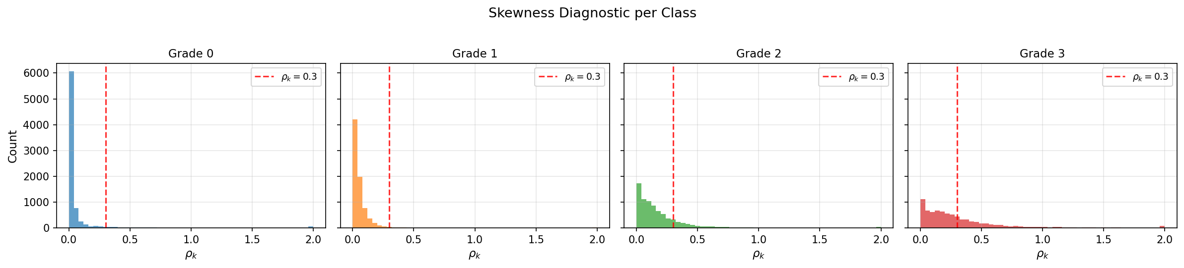
These statistics explain the BNN ranking in Table ¿tbl:tab:selective-bnn?: with the majority of critical-class \(C_k\) estimates reliable, \(C_{\text{crit\_max}}\) can exploit the per-class signal effectively. The MC dropout model (Appendix 10.12) produces coarser posterior samples (fewer effective degrees of freedom), inflating \(\rho_k\) and degrading \(C_k\) for critical classes, which explains why CBEC, whose correlation gate is Taylor-free and whose restricted domain \(\mathcal{S}\times\mathcal{C}\) filters irrelevant co-elevation, outperforms \(C_{\text{crit\_max}}\) in that regime.
10.5 Class-Imbalance Stress Test↩︎
To isolate the effect of class prevalence on the decomposition, we ran a controlled four-class FashionMNIST subset experiment in which the training prevalence of one target class was reduced from \(100\%\) to \(10\%\), while keeping labels clean, the architecture fixed, and the test set balanced. As the target class becomes rarer, its mean prediction decreases (\(\mu_k: 0.933 \to 0.734\)), raw variance increases (\(1.42{\times}10^{-3} \to 3.82{\times}10^{-3}\)), and the normalised contribution \(C_k\) increases more strongly (\(1.47{\times}10^{-3} \to 6.12{\times}10^{-3}\)). Approximation quality deteriorates only gradually: the target-class \(\rho_k\) increases from \(0.025\) to \(0.129\), the absolute gap \(|\sum_k C_k-\mathcal{I}|\) increases from \(5.4{\times}10^{-4}\) to \(9.8{\times}10^{-4}\), and the reliable fraction remains high, decreasing from \(99.2\%\) to \(93.9\%\). Thus class imbalance makes the boundary-aware normalisation more important, but prevalence alone does not determine reliability; \(\rho_k\) remains the appropriate diagnostic.
10.6 Theory Validation: MI vs.\(\sum_k C_k\)↩︎
Figure 4 plots \(\sum_k C_k\) against exact MI for all 7,948 test samples, complementing the summary statistics reported in Section 3.3. The slight systematic overestimation visible at high MI values is consistent with the third-order correction in Lemma 4: right-skewed distributions near the simplex boundary produce \(m_{3,k} > 0\), and the omitted correction \(-\frac{1}{6}\sum_k m_{3,k}/\mu_k^2\) causes \(\sum_k C_k\) to slightly exceed MI. The right panel confirms this: residuals \((\sum_k C_k - \mathrm{MI})\) are predominantly positive for high-skewness samples (pink/red points), validating that the skewness diagnostic \(\rho_k\) correctly identifies inputs where the approximation degrades.
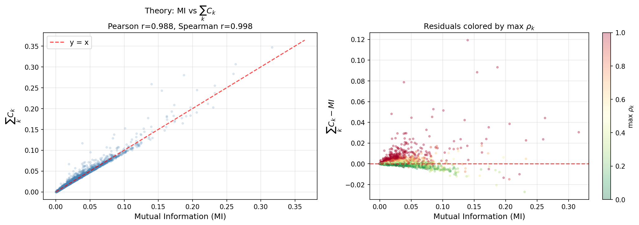
10.7 Extended Selective Prediction Analysis↩︎
Figure 5 shows the full selective risk curves for all 10 deferral policies across continuous coverage levels. The left panel (Critical FNR) confirms that \(C_{\text{crit\_max}}\) achieves the lowest AUSC (0.285), with \(C_{\text{crit\_sum}}\) second (0.329) and CBEC third (0.415). The gap widens at lower coverages where clinical operating points typically lie, and the unnormalised variance baselines (Sale_EU_crit: 0.650, Var_crit: 0.606) perform substantially worse than even scalar MI (0.436), confirming that boundary suppression severely degrades raw variance for rare critical classes.
The right panel addresses a natural concern: does targeting critical-class uncertainty sacrifice overall accuracy? The answer is no. \(C_{\text{crit\_max}}\) achieves competitive error-rate AUSC (0.143), comparable to entropy (0.127) and MaxProb (0.126), which optimise for overall accuracy rather than safety. This demonstrates that the \(C_k\) decomposition identifies samples where critical-class confusion drives errors, rather than deferring difficult samples indiscriminately.
A further distinction emerges at the clinically relevant 80% coverage point: \(C_{\text{crit\_max}}\) retains 1,293 critical samples (27.2% deferred) while achieving FNR \(0.302\), whereas MI retains only 1,183 (33.4% deferred) with FNR \(0.339\). \(C_{\text{crit\_max}}\) is simultaneously less aggressive at deferring critical cases and more accurate on those it keeps, the hallmark of a well-targeted deferral policy. Entropy, by contrast, defers 42.1% of critical samples at 80% coverage because it prioritises total uncertainty rather than critical-class epistemic uncertainty.
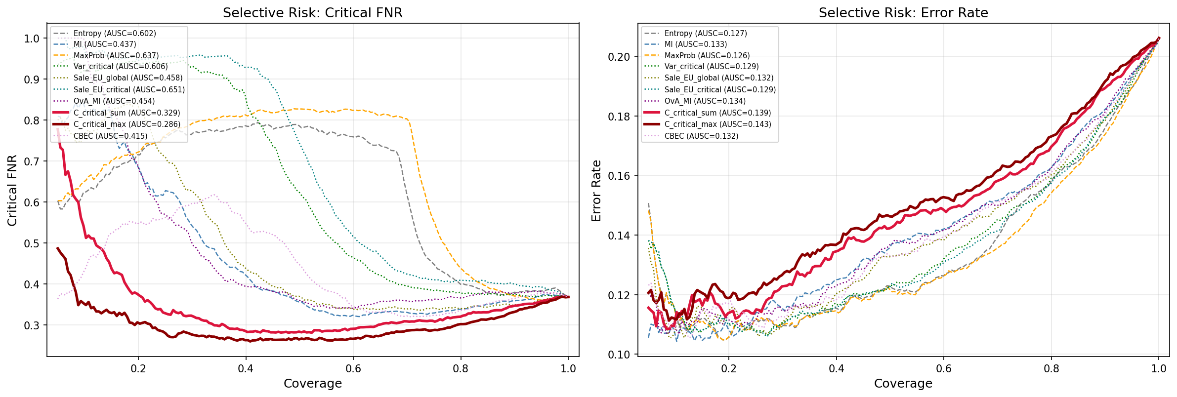
10.8 Full Bootstrap Results: Bayesian Model↩︎
Table 7 extends Table ¿tbl:tab:selective-bnn? with all evaluated policies and additional metrics at 80% coverage. The ranking stability column reports the fraction of 200 bootstrap resamples in which each policy achieves the lowest AUSC.5
| Family | Policy | AUSC\(\downarrow\) | Critical FNR @80%\(\downarrow\) | Acc @80%\(\uparrow\) | Win% |
|---|---|---|---|---|---|
| Per-class \(C_k\) | \(C_{\text{crit\_max}}\) | \(0.285 \pm 0.016\) | \(0.302 \pm 0.013\) | \(0.827 \pm 0.005\) | 50.5 |
| Per-class \(C_k\) | \(C_{\text{crit\_sum}}\) | \(0.327 \pm 0.017\) | \(0.321 \pm 0.014\) | \(0.831 \pm 0.005\) | 0.0 |
| Boundary | CBEC | \(0.416 \pm 0.020\) | \(0.335 \pm 0.014\) | \(0.840 \pm 0.005\) | 0.0 |
| Scalar | MI | \(0.436 \pm 0.019\) | \(0.339 \pm 0.014\) | \(0.838 \pm 0.005\) | 0.0 |
| Per-class MI | OvA_MI | \(0.452 \pm 0.017\) | \(0.367 \pm 0.015\) | \(0.838 \pm 0.005\) | 0.0 |
| Per-class var. | Sale_EU_global | \(0.457 \pm 0.018\) | \(0.341 \pm 0.015\) | \(0.840 \pm 0.005\) | 0.0 |
| Scalar | Entropy | \(0.604 \pm 0.022\) | \(0.401 \pm 0.016\) | \(0.842 \pm 0.005\) | 0.0 |
| Per-class var. | Var_crit | \(0.606 \pm 0.014\) | \(0.379 \pm 0.016\) | \(0.842 \pm 0.005\) | 0.0 |
| Scalar | MaxProb | \(0.639 \pm 0.022\) | \(0.439 \pm 0.017\) | \(0.846 \pm 0.005\) | 0.0 |
| Per-class var. | Sale_EU_crit | \(0.650 \pm 0.013\) | \(0.409 \pm 0.016\) | \(0.843 \pm 0.005\) | 0.0 |
10.8.0.1 Pairwise statistical significance.
Table 8 reports bootstrap pairwise comparisons for the proposed methods against key baselines. \(P(\text{row} < \text{col})\) denotes the fraction of bootstrap resamples in which the row policy achieves lower AUSC than the column policy; values above 0.975 indicate significance at the 5% level (two-tailed).
| MI | Var_crit | Sale_EU_crit | |
|---|---|---|---|
| \(C_{\text{crit\_max}}\) | \(1.000^{***}\) | \(1.000^{***}\) | \(1.000^{***}\) |
| \(C_{\text{crit\_sum}}\) | \(1.000^{***}\) | \(1.000^{***}\) | \(1.000^{***}\) |
| CBEC | \(0.950\) | \(1.000^{***}\) | \(1.000^{***}\) |
10.9 Epistemic Profiles↩︎
Table 9 reports the normalised epistemic mass \(\mathbb{E}[C_k / \sum_j C_j \mid y = i]\), showing which classes absorb epistemic uncertainty for each true label. Figure 6 visualises both the raw and normalised profiles as heatmaps.
![Figure 6: Epistemic profiles. Left: Raw \mathbb{E}[C_k \mid y{=}i]. Right: Normalised \mathbb{E}[C_k / \sum_j C_j \mid y{=}i]. Grade 2 dominates the epistemic budget across all true classes, identifying moderate DR as the model’s primary source of confusion.](/article/2602.21160/figures/diagnostic_epistemic_profiles.png "fig:")
| True class | \(C_0\) | \(C_1\) | \(C_2\) | \(C_3\) |
|---|---|---|---|---|
| Grade 0 | 12.3% | 32.7% | 50.9% | 4.0% |
| Grade 1 | 22.0% | 24.8% | 47.1% | 6.1% |
| Grade 2 | 34.6% | 18.2% | 31.0% | 16.2% |
| Grade 3 | 21.4% | 15.7% | 40.2% | 22.7% |
Grade 2 is the dominant source of epistemic uncertainty across all true classes, consistent with it being the most confusable category (moderate DR is clinically subtle). For true Grade 0 and Grade 1, over 50% and 47% of the epistemic mass concentrates on \(C_2\) respectively, indicating the model’s primary source of doubt about safe-class images is whether they might be moderate DR. For true Grade 3, the epistemic mass is split between \(C_2\) (40.2%) and \(C_3\) (22.7%), reflecting the severity continuum. Grade 2 is also the dominant epistemic class (\(\arg\max_k C_k\)) for 64.9% of all test samples, confirming that moderate DR is the model’s primary source of confusion at the individual-input level as well.
10.10 Error Signatures↩︎
A distinctive advantage of \(\boldsymbol{C}(x)\) over scalar MI is that it fingerprints the structure of model confusion. Figure 7 shows \(\mathbb{E}[C_k \mid y{=}i, \hat{y}{=}j]\) for five clinically important outcomes, and Table 10 provides the numerical values.
![Figure 7: Epistemic signatures of error types. Each bar shows \mathbb{E}[C_k \mid y{=}i, \hat{y}{=}j] for class k \in \{0,1,2,3\}. Catastrophic misses (3 \to 0) and severity errors (3 \to 2) have similar MI but distinct C_k fingerprints, revealing different confusion pathways invisible to scalar metrics.](/article/2602.21160/figures/paper_error_signatures_bootstrap_bnn.png "fig:")
| Error | \(n\) | MI | \(C_0\) | \(C_1\) | \(C_2\) | \(C_3\) | Dominant |
|---|---|---|---|---|---|---|---|
| \(3 \to 0\) (catastrophic) | 107 | 0.024 | 0.008 | 0.002 | 0.012 | 0.002 | \(C_2\) |
| \(3 \to 2\) (severity) | 220 | 0.027 | 0.013 | 0.004 | 0.005 | 0.008 | \(C_0\) |
| \(2 \to 0\) (missed treat.) | 548 | 0.025 | 0.008 | 0.002 | 0.013 | 0.002 | \(C_2\) |
| \(3 \to 3\) (correct) | 128 | 0.026 | 0.002 | 0.002 | 0.017 | 0.007 | \(C_2\) |
| \(0 \to 0\) (correct conf.) | 5447 | 0.012 | 0.003 | 0.002 | 0.007 | 0.001 | \(C_2\) |
The key interpretability result is that errors with similar scalar MI have distinctive \(C_k\) fingerprints. Catastrophic misses (true Grade 3 predicted as Grade 0, \(n{=}107\)) and severity underestimates (true Grade 3 predicted as Grade 2, \(n{=}220\)) have nearly identical scalar MI (\(0.024\) vs.\(0.027\) nats) but quite different \(C_k\) signatures. The catastrophic miss concentrates epistemic mass on \(C_2\): the model does not jump directly from severe to healthy, but routes through moderate DR, identifying Grade 2 as the “bottleneck” of confusion. The severity underestimate instead elevates \(C_0\), indicating the model’s primary doubt is whether the image might be healthy. These qualitatively different failure modes, invisible to any scalar metric, suggest distinct intervention strategies: additional moderate-vs-severe training data for the first, and better healthy-vs-severe discrimination for the second.
10.11 Epistemic Confusion Matrix↩︎
Figure 8 visualises the epistemic confusion matrix \(E_{ij} = \mathbb{E}[\sqrt{C_i C_j}\,\max(0,-\rho_{ij})]\), which quantifies pairwise confusion between classes using the same correlation-gated geometric mean that underlies CBEC (Eq. 12 ). Table 11 provides the numerical values.
The cross-boundary block (safe\(\times\)critical) dominates: its mean value is \(2.7\times\) the within-safe mean and \(10.6\times\) the within-critical mean, confirming that the model’s epistemic uncertainty concentrates at the clinically dangerous boundary. The strongest pairwise confusion is Grade 0\(\leftrightarrow\)Grade 2 (\(5.08 \times 10^{-3}\)), consistent with the epistemic profiles (Table 9) showing Grade 2 as the dominant source of uncertainty for healthy images. This structure validates both the safe/critical partition and the CBEC aggregation, which specifically targets cross-boundary confusion.
![Figure 8: Epistemic confusion matrix E_{ij} = \mathbb{E}[\sqrt{C_i C_j}\,\max(0,-\rho_{ij})]. The cross-boundary block (safe\timescritical, blue outline) dominates, with the Grade 0\leftrightarrowGrade 2 pair (5.08 \times 10^{-3}) exhibiting the strongest confusion. Within-critical confusion is an order of magnitude weaker (10.6\times smaller mean), confirming that the model’s epistemic uncertainty concentrates at the clinically dangerous safe/critical boundary.](/article/2602.21160/figures/diagnostic_confusion_matrix.png "fig:")
| Gr. 0 | Gr. 1 | Gr. 2 | Gr. 3 | |
|---|---|---|---|---|
| Grade 0 | 0.00 | 1.54 | 5.08 | 2.37 |
| Grade 1 | 1.54 | 0.00 | 0.21 | 0.52 |
| Grade 2 | 5.08 | 0.21 | 0.00 | 0.39 |
| Grade 3 | 2.37 | 0.52 | 0.39 | 0.00 |
10.12 Full Bootstrap Results: MC Dropout↩︎
Table 12 reports the MC dropout evaluation. The ranking reversal relative to the BNN (Table 7) is consistent with both the skewness analysis (Appendix 10.4) and the findings of [14], who showed that MC dropout underestimates posterior uncertainty and creates regions of spurious confidence. The coarser posterior samples inflate \(\rho_k\) for critical classes, degrading the reliability of individual \(C_k\) values and hence \(C_{\text{crit\_max}}\), while leaving CBEC’s correlation-gated structure intact, since CBEC computes correlations directly from the MC draws rather than relying on the second-order approximation.
| Family | Policy | AUSC\(\downarrow\) | Critical FNR @80%\(\downarrow\) | Acc @80%\(\uparrow\) |
|---|---|---|---|---|
| Boundary | CBEC | \(\mathbf{0.197 \pm 0.012}\) | \(0.316 \pm 0.015\) | \(0.867 \pm 0.004\) |
| Scalar | Entropy | \(0.249 \pm 0.017\) | \(\mathbf{0.294 \pm 0.014}\) | \(0.871 \pm 0.004\) |
| Scalar | MaxProb | \(0.268 \pm 0.017\) | \(0.340 \pm 0.016\) | \(0.874 \pm 0.004\) |
| Per-class var. | Sale_EU_global | \(0.364 \pm 0.022\) | \(0.410 \pm 0.018\) | \(0.870 \pm 0.004\) |
| Per-class \(C_k\) | \(C_{\text{crit\_max}}\) | \(0.419 \pm 0.025\) | \(0.390 \pm 0.017\) | \(0.854 \pm 0.004\) |
| Per-class var. | Var_crit | \(0.424 \pm 0.026\) | \(0.451 \pm 0.018\) | \(0.868 \pm 0.004\) |
| Scalar | MI | \(0.425 \pm 0.024\) | \(0.459 \pm 0.019\) | \(0.864 \pm 0.004\) |
| Per-class \(C_k\) | \(C_{\text{crit\_sum}}\) | \(0.436 \pm 0.026\) | \(0.404 \pm 0.017\) | \(0.860 \pm 0.004\) |
| Per-class var. | Sale_EU_crit | \(0.463 \pm 0.027\) | \(0.527 \pm 0.019\) | \(0.866 \pm 0.004\) |
| Per-class MI | OvA_MI | \(0.526 \pm 0.028\) | \(0.556 \pm 0.020\) | \(0.861 \pm 0.004\) |
CBEC reduces AUSC by 53.6% relative to MI (\(0.197\) vs.\(0.425\)) and wins 100% of bootstrap samples. Scalar entropy (\(0.249\)) outperforms all epistemic methods including MI (\(0.425\)) under MC dropout; this is because entropy captures total uncertainty (aleatoric + epistemic), and under MC dropout’s coarser posterior, the aleatoric component carries complementary signal that pure epistemic measures miss. \(C_{\text{crit\_max}}\) still outperforms its unnormalised counterpart Sale_EU_crit (\(0.419\) vs.\(0.463\)), confirming that the \(1/\mu_k\) normalisation provides benefit even when the Taylor approximation is degraded.
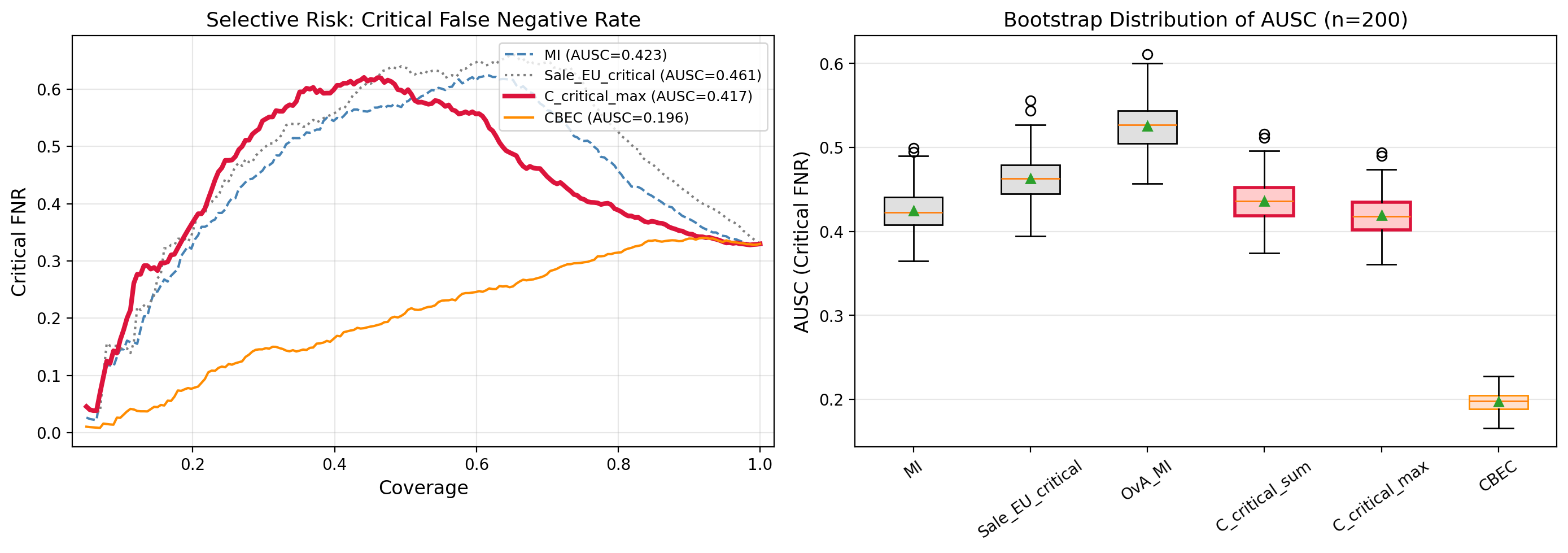
10.12.0.1 Why \(C_k\) degrades under MC dropout: a skewness analysis.
Figure 10 reveals the mechanism behind \(C_{\text{crit\_max}}\)’s ranking reversal. Under the low-rank BNN, the fraction of samples with reliable \(C_k\) (\(\rho_k < 0.3\)) remains above \(80\%\) for Grades 0–2 and drops to \(63\%\) only for Grade 3 (Severe/PDR), the rarest and most difficult class. Under MC dropout, the same statistic degrades monotonically with clinical severity: \(88\%\) (Grade 0), \(72\%\) (Grade 1), \(54\%\) (Grade 2), and only \(22\%\) (Grade 3).
The right panel quantifies the gap. Median \(\rho_k\) is comparable between the two models at Grade 0 (\(0.013\) vs.\(0.012\)), where both posteriors are well-behaved. The gap widens progressively: at Grade 1, MC dropout’s median \(\rho_k\) is \(3.5\times\) higher than the BNN’s (\(0.130\) vs.\(0.037\)); at Grade 2 it is \(2.1\times\) higher (\(0.264\) vs.\(0.124\)); and at Grade 3 the MC dropout median exceeds the reliability boundary entirely (\(1.125\) vs.\(0.218\)). For the most safety-critical class, more than three quarters of MC dropout samples operate in the regime where the second-order Taylor approximation has broken down. This pattern is consistent with MC dropout’s known tendency to underestimate tail variance [14]: the resulting predictive distributions are more concentrated than the true posterior, but with heavier skewness, pushing \(\rho_k\) above the reliability threshold precisely for the classes that matter most.
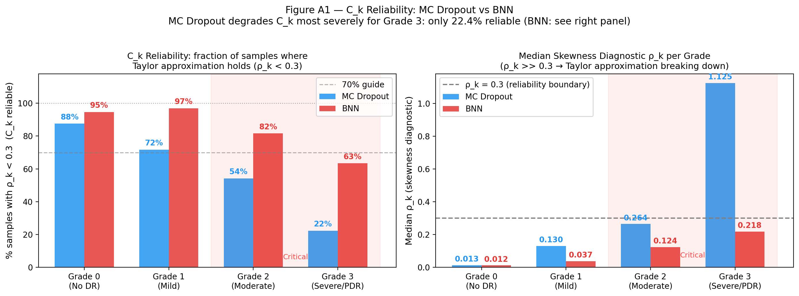
These results provide direct empirical support for the complementarity claimed in Section 3: \(C_{\text{crit\_max}}\) is the preferred deferral metric under well-calibrated posteriors where \(\rho_k\) remains low, while CBEC provides a robust fallback when the posterior approximation inflates skewness beyond the Taylor regime. The skewness diagnostic \(\rho_k\) therefore serves as a practical model-selection criterion: if median \(\rho_k\) for the critical classes exceeds \(0.3\), practitioners should prefer CBEC over \(C_{\text{crit\_max}}\).
10.13 Deep Ensemble Validation: Per-Class Metrics↩︎
To verify that the benefit of the \(1/\mu_k\) normalisation persists across inference paradigms, we evaluate a deep ensemble of five members on the same diabetic retinopathy test set (\(7{,}948\) images), using the identical evaluation pipeline. Each member shares the Phase 1 EfficientNet-B4 backbone and is fine-tuned independently with a different random seed; diversity arises from head initialisation rather than stochastic inference. We restrict the comparison to MI as the scalar epistemic reference and the full per-class family: raw per-class variance baselines from [7] and our proposed \(C_k\) metrics.
10.13.0.1 Reliability.
The deep ensemble achieves near-uniform \(C_k\) reliability across all DR grades: \(95.7\%\), \(91.2\%\), \(91.5\%\), and \(85.1\%\) of samples satisfy \(\rho_k < 0.3\) for Grades 0–3 respectively. This places the ensemble firmly in the high-reliability regime, in contrast to MC dropout where Grade 3 reliability collapses to \(22\%\) (Figure 10).
10.13.0.2 Results.
Table 13 reports AUSC and critical FNR at \(80\%\) coverage over 200 bootstrap resamples.
| Policy | AUSC\(\downarrow\) | Crit.FNR @80%\(\downarrow\) |
|---|---|---|
| Var_crit | \(0.408 \pm 0.030\) | \(0.362 \pm 0.017\) |
| Sale_EU_crit [7] | \(0.447 \pm 0.031\) | \(0.414 \pm 0.018\) |
| \(C_{\text{crit\_max}}\) | \(0.390 \pm 0.029\) | \(0.314 \pm 0.016\) |
| \(C_{\text{crit\_sum}}\) | \(0.406 \pm 0.029\) | \(0.333 \pm 0.016\) |
| CBEC | \(\mathbf{0.223 \pm 0.018}\) | \(\mathbf{0.237 \pm 0.013}\) |
Two findings are consistent across all three inference regimes. First, \(C_{\text{crit\_max}}\) outperforms its unnormalised counterpart \(\text{Sale\_EU\_crit}\) by \(12.9\%\) in AUSC (\(0.390\) vs.\(0.447\)), confirming that the \(1/\mu_k\) normalisation provides a systematic advantage over raw per-class variance regardless of the inference method. Second, CBEC achieves the lowest AUSC and critical FNR, outperforming MI by \(37.0\%\) (\(0.223\) vs.\(0.354\)) and both Sale et al.variants on every metric. Notably, all three proposed \(C_k\) metrics outperform Sale_EU_crit, their direct unnormalised counterpart, confirming the boundary-correction benefit of the \(1/\mu_k\) normalisation even in the high-reliability ensemble regime where the Taylor approximation is near-exact (\(\sum_k C_k / \text{MI} = 0.996\) on this test set).
11 OoD Detection Experiment: Supplementary Details↩︎
11.1 Datasets and Preprocessing↩︎
11.1.0.1 FashionMNIST \(\to\) KMNIST.
FashionMNIST [28] comprises 60,000 grayscale images (\(28 \times 28\)) across 10 clothing categories; in
code, the 60,000 training images are split into 50,000 train and 10,000 validation, and the standard 10,000 FashionMNIST test set is used as the in-distribution test set. KMNIST [29] provides 10,000 test images of cursive Japanese characters in the same format, used entirely as OoD data. Preprocessing is identical for ID/OoD images: cast to float32,
normalized by dividing pixel values by 126, and flattened each \(28\times 28\) image to a 784-dimensional vector; no data augmentation is used.
11.1.0.2 MIMIC-III ICU \(\to\) Newborn.
We extract adult ICU admissions from MIMIC-III [30], yielding 44 clinical features with binary mortality labels, split into train/test =
40,406/4,490. The Newborn unit (5,357 admissions) serves as OoD data. The 44-feature pipeline merges (on SUBJECT_ID, HADM_ID, ICUSTAY_ID): (i) static patient features (including age, ICU LOS, pre-ICU hospital time,
gender one-hot), (ii) per-stay mean/std aggregates of mapped vital-sign ITEMIDs, and (iii) per-stay mean/std aggregates of mapped lab ITEMIDs restricted to timestamps within ICU stay. Newborn admissions are excluded from ID data and kept as OoD. Adult-ID
preprocessing applies an 8\(\times\)IQR outlier filter, plausibility filters (mean_combined_bp_dia and mean_combined_bp_sys \(>10\),
time_at_hosp_pre_ic_admission \(>0\)), fills missing std-feature entries with 0, then uses median imputation and MinMax scaling fit on train and applied to test/OoD. In the OoD loader used for experiments,
newborn age (and weight, if present) are set to the adult-training mean values before evaluation.
11.2 Model Architecture and Training↩︎
Both tasks use fully connected Bayesian neural networks with ReLU activations and low-rank Gaussian posteriors. Output layers are linear (no activation), trained with logits, and mapped to class probabilities via softmax at inference. All models share the following configuration:
11.2.0.1 Shared specification.
The prior is a scale-mixture Gaussian [37] with \(\pi{=}0.5\), \(\sigma_1{=}1.0\), \(\sigma_2{=}\exp(-6)\). Posterior initialisation is adaptive per layer: \(\sigma_w^2 = 2/d_{\text{in}}\) for ReLU layers, \(2/(d_{\text{in}}{+}d_{\text{out}})\) otherwise; damping is \(0.55\) for \(r > 5\) (else \(0.32\)); factor means \(A_\mu, B_\mu \sim \mathcal{U}(-a, a)\) with \(a = \text{damping}\sqrt{3}(\sigma_w^2/r)^{1/4}\); bias means \(b_\mu = 0\); and \(A_\rho, B_\rho, b_\rho\) are set to constant \(\rho_{\text{init}} = \log(\exp(\sigma_{\text{init}}) - 1)\) with \(\sigma_{\text{init}} = 0.09(\sigma_w^2/r)^{1/4}\). All models are trained with Adam at learning rate \(10^{-3}\).
11.2.0.2 Per-task details.
Table 14 summarises the task-specific hyperparameters.
| FashionMNIST | MIMIC-III | |
|---|---|---|
| Hidden layers | \(2 \times 1{,}200\) | \(2 \times 128\) |
| Rank \(r\) | 25 | 15 |
| Output classes | 10 | 2 |
| Batch size | 128 | 64 |
| Epochs | 50 | 256 |
| KL schedule | Linear warmup, 10 epochs | Fixed |
| KL scale | \(0 \to 1/N_{\text{train}}\) | \(0.5/\lceil N_{\text{train}}/\text{batch}\rceil\) |
| Class weighting | None | \(w_0{=}1,\; w_1{=}1/\text{pos\_frac} \approx 11.9\) |
| MC samples \(S\) | 50 | 512 |
Results are reported as mean \(\pm\) std over 5 independent training seeds.
11.3 Extended OoD Detection Results↩︎
Table 15 reports per-metric distributional statistics for both benchmarks. On FashionMNIST, MI and \(EU_{\text{var}}\) share the same OoD/ID ratio (\(5.92\times\)) but MI achieves higher AUROC because its absolute values provide better threshold separation. On MIMIC-III, \(EU_{\text{var}}\) has the highest ratio (\(1.71\times\)) yet the lowest AUROC among epistemic measures (\(0.778\)), confirming that ratio alone does not determine detection performance when the dynamic range of scores is compressed by boundary suppression.
| Dataset | Metric | Mean (ID) | Mean (OoD) | Ratio\(\uparrow\) |
|---|---|---|---|---|
| FashionMNIST | Neg.MSP | 0.0506 | 0.1043 | 2.07 |
| MI | 0.0096 | 0.0569 | 5.92 | |
| \(EU_{\text{var}}\) | 0.0056 | 0.0333 | 5.92 | |
| \(\sum_k C_k\) | 0.0106 | 0.0677 | 6.43 | |
| MIMIC-III | Neg.MSP | 0.2543 | 0.3150 | 1.24 |
| MI | 0.0378 | 0.0598 | 1.61 | |
| \(EU_{\text{var}}\) | 0.0289 | 0.0485 | 1.71 | |
| \(\sum_k C_k\) | 0.0377 | 0.0601 | 1.62 |
11.3.0.1 Per-class decomposition (MIMIC-III).
The binary setting permits direct inspection of per-class contributions: \(\sum_k C_k = C_0 + C_1\). Table 16 reveals that distributional shift affects the two classes asymmetrically. The survival class exhibits a \(2.15\times\) increase from ID to OoD (\(C_0\): \(0.014 \to 0.030\)), while the mortality class shows only \(1.30\times\) (\(C_1\): \(0.022 \to 0.029\)). The critical-class-only metric \(C_1\) achieves AUROC \(0.740 \pm 0.074\), substantially below \(\sum_k C_k\) at \(0.815 \pm 0.017\): by focusing exclusively on mortality-class uncertainty, it misses the larger OoD signal carried by \(C_0\). This illustrates a task-dependent trade-off: \(C_{\text{crit\_max}}\) targets safety-critical selective prediction (Section 3), where critical-class uncertainty directly determines clinical harm; for general OoD detection, all-class aggregation captures the complete distributional shift.
| Metric | Mean (ID) | Mean (OoD) | Ratio\(\uparrow\) | AUROC\(\uparrow\) |
|---|---|---|---|---|
| \(C_0\) (survival) | 0.014 | 0.030 | 2.15 | \(0.773 \pm 0.005\) |
| \(C_1\) (mortality) | 0.022 | 0.029 | 1.30 | \(0.740 \pm 0.074\) |
| \(\sum_k C_k\) | 0.038 | 0.060 | 1.62 | \(\mathbf{0.815 \pm 0.017}\) |
11.4 Per-Class Epistemic Decomposition for FashionMNIST↩︎
The main text reports \(\sum_k C_k\) as the best OoD metric for FashionMNIST\(\to\)KMNIST (AUROC \(0.735 \pm 0.009\)) but presents only the scalar aggregate. Figure 11 decomposes this into the ten individual \(C_k\) values, revealing which clothing categories drive the OoD signal when the model encounters KMNIST inputs.
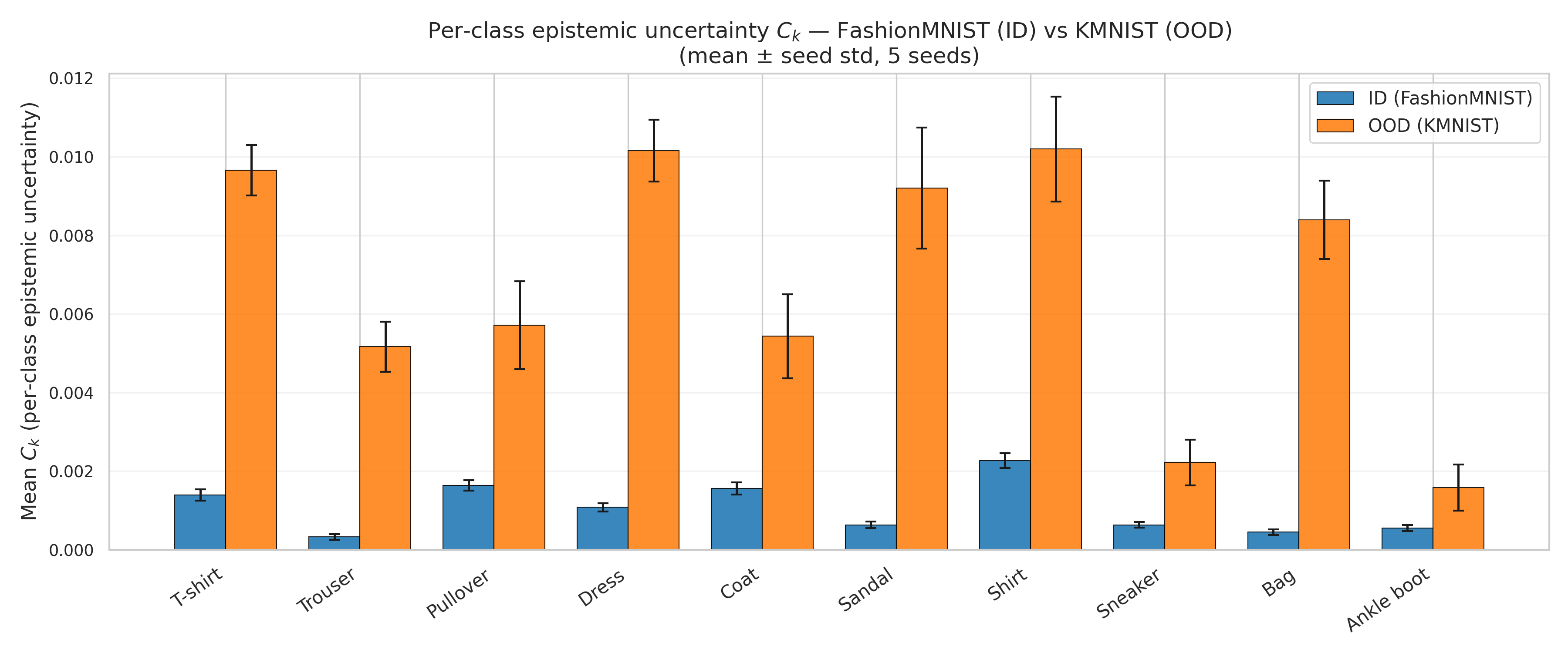
Table 17 reports the numerical values for each class.
| Class | \(\bar{C}_k^{\text{ID}}\) | \(\sigma^{\text{ID}}\) | \(\bar{C}_k^{\text{OoD}}\) | \(\sigma^{\text{OoD}}\) | Ratio |
|---|---|---|---|---|---|
| T-shirt/top | 0.00140 | 0.00014 | 0.00966 | 0.00064 | 6.92 |
| Trouser | 0.00033 | 0.00007 | 0.00517 | 0.00064 | 15.65 |
| Pullover | 0.00164 | 0.00013 | 0.00571 | 0.00112 | 3.49 |
| Dress | 0.00108 | 0.00010 | 0.01015 | 0.00079 | 9.37 |
| Coat | 0.00156 | 0.00015 | 0.00543 | 0.00106 | 3.48 |
| Sandal | 0.00064 | 0.00008 | 0.00920 | 0.00154 | 14.43 |
| Shirt | 0.00228 | 0.00019 | 0.01020 | 0.00133 | 4.48 |
| Sneaker | 0.00064 | 0.00007 | 0.00222 | 0.00058 | 3.49 |
| Bag | 0.00045 | 0.00007 | 0.00840 | 0.00099 | 18.67 |
| Ankle boot | 0.00056 | 0.00008 | 0.00158 | 0.00058 | 2.85 |
| \(\sum_k C_k\) (aggregate) | 0.01056 | - | 0.06773 | - | 6.43 |
We additionally evaluate each individual \(C_k(x)\) as a scalar OoD score. Table 18 shows that every class provides non-trivial ID/OoD separation, with AUROC ranging from \(0.537\) for Ankle boot to \(0.683\) for Bag. These per-class AUROCs remain below the aggregate \(\sum_k C_k\) AUROC of \(0.735 \pm 0.009\), confirming that the shift is broad enough that aggregation is the strongest detector, while the individual components reveal where the shift is concentrated.
| Class | OoD/ID ratio | AUROC using \(C_k\) |
|---|---|---|
| T-shirt/top | \(6.971 \pm 0.788\) | \(0.670 \pm 0.027\) |
| Trouser | \(16.046 \pm 2.370\) | \(0.656 \pm 0.024\) |
| Pullover | \(3.477 \pm 0.549\) | \(0.578 \pm 0.020\) |
| Dress | \(9.428 \pm 1.005\) | \(0.662 \pm 0.020\) |
| Coat | \(3.481 \pm 0.602\) | \(0.577 \pm 0.026\) |
| Sandal | \(14.729 \pm 3.755\) | \(0.650 \pm 0.019\) |
| Shirt | \(4.467 \pm 0.337\) | \(0.615 \pm 0.025\) |
| Sneaker | \(3.494 \pm 0.906\) | \(0.549 \pm 0.054\) |
| Bag | \(18.854 \pm 2.173\) | \(0.683 \pm 0.030\) |
| Ankle boot | \(2.921 \pm 1.439\) | \(0.537 \pm 0.050\) |
For reference, the aggregate \(\sum_k C_k\) achieves an OoD/ID mean-score ratio of \(6.43\times\) (vs.\(5.92\times\) for MI and \(5.92\times\) for \(EU_{\text{var}}\)), confirming that the \(\mu_k\)-normalisation in \(C_k\) provides a consistent boost over the raw variance sum.
11.5 Score Distribution Analysis and the \(EU_{\text{var}}\) Paradox↩︎
On MIMIC-III, \(EU_{\text{var}}\) achieves the highest mean OoD/ID ratio (\(1.705\times\)) yet the lowest AUROC (\(0.778\)) among the three primary Bayesian metrics. Figure 12 makes this paradox immediately visual.
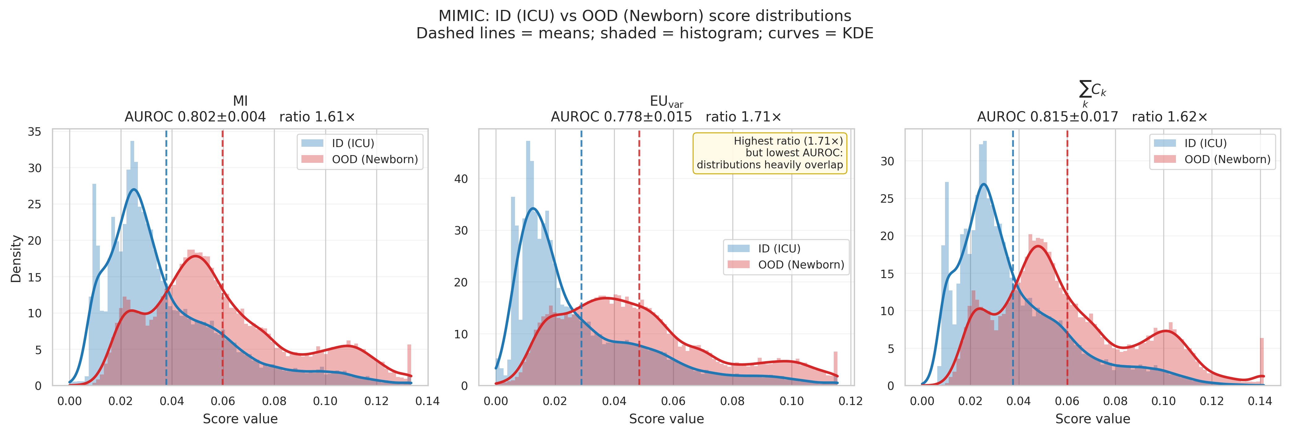
11.5.0.1 Why a high mean ratio does not imply better separability.
AUROC measures \(P(s_{\mathrm{OoD}} > s_{\mathrm{ID}})\) for a randomly chosen pair drawn independently from the OoD and ID score distributions. This probability is governed by the full distributional overlap, not merely the ratio of means. Under a Gaussian approximation of the log-scores, the relationship is \[\mathrm{AUROC} \;\approx\; \Phi\!\left( \frac{\mu_{\mathrm{OoD}} - \mu_{\mathrm{ID}}}{\sqrt{\sigma^2_{\mathrm{OoD}} + \sigma^2_{\mathrm{ID}}}} \right), \label{eq:auroc95gaussian95approx}\tag{37}\] where \(\Phi\) is the standard-normal CDF. A high OoD/ID mean ratio inflates the numerator, but if the within-group standard deviations are also large, the denominator grows proportionally and the AUROC gain is suppressed, analogous to Cohen’s \(d\).
11.5.0.2 Why EU\(_{\mathrm{var}}\) suffers from dynamic range compression.
EU\(_{\mathrm{var}} = \sum_k \mathrm{Var}[p_k]\) is an un-normalised variance sum. For a sigmoid binary classifier, predictive variance is heteroscedastic: samples near the decision boundary have high \(\mathrm{Var}[p_k]\) irrespective of ID/OoD status, simultaneously inflating the right tail of both distributions. Although the OoD mean exceeds the ID mean by a factor of \(1.71\times\), the bulk of both distributions concentrates near zero with only a thin right tail separating them. The resulting large within-group spread keeps the denominator of 37 large, yielding the lowest AUROC (\(0.778\)) among the three Bayesian metrics.
11.5.0.3 Why \(\sum_k C_k\) achieves better separation with a lower ratio.
\(C_k = \mathrm{Var}[p_k]\,/\,(2\mu_k)\) normalises each variance component by the corresponding mean probability. This acts as a variance-stabilising transform: large absolute variances that arise when \(\mu_k\) is also large are down-weighted, while contributions from classes with small \(\mu_k\) are amplified. The net effect narrows the within-group spread for both ID and OoD populations, so a smaller mean ratio (\(1.62\times\) vs.\(1.71\times\)) still translates to cleaner tail separation and a higher AUROC (\(0.815\)).
11.5.0.4 Why the paradox is absent on FashionMNIST.
On FashionMNIST\(\to\)KMNIST, \(EU_{\text{var}}\) and MI attain nearly identical mean ratios (\(5.923\times\) vs.\(5.921\times\)), and their AUROC gap is only \(0.014\). The distinction arises because KMNIST induces a strong, directionally consistent uncertainty lift across all ten softmax outputs, preventing the range compression that afflicts \(EU_{\text{var}}\) on MIMIC’s binary sigmoid output.
11.6 Empirical Verification of the Skewness Diagnostic↩︎
Lemma 4 establishes that the expected entropy satisfies \[\mathbb{E}\bigl[\mathcal{H}(\mathbf{p})\bigr] \;\approx\; \mathcal{H}(\boldsymbol{\mu}) - \frac{1}{2}\sum_k \frac{\mathrm{Var}[p_k]}{\mu_k} + \frac{1}{6}\sum_k \frac{m_{3,k}}{\mu_k^2}, \label{eq:lem3}\tag{38}\] where \(m_{3,k} = \frac{1}{S}\sum_{s=1}^S(p_k^{(s)} - \mu_k)^3\) is the empirical third central moment. The reliability of the second-order approximation (i.e.\(\sum_k C_k\)) is governed by the skewness diagnostic \[\rho_k(x) = \frac{|m_{3,k}|}{3\,\mu_k \cdot \mathrm{Var}[p_k]} = \frac{\bigl|\text{3rd-order correction}\bigr|}{\bigl|\text{2nd-order correction}\bigr|}, \label{eq:rho95app}\tag{39}\] so \(\rho_k < 1\) signals a reliable quadratic regime and \(\rho_k \gg 1\) signals regime breakdown. Note that \(3\mu_k \cdot \mathrm{Var}[p_k] = 6\mu_k^2 C_k\), so \(\rho_k = |m_{3,k}| / (6\mu_k^2 C_k)\): the \(1/\mu_k^2\) factor amplifies \(\rho_k\) for classes with small predicted probability, which is precisely the singularity avoided by using \(C_k\) rather than \(C_k^{(3)}\).
The main text claims OoD inputs have higher \(\rho_k\) than ID inputs. Figures 13 and 14 provide the first direct empirical confirmation, with one instructive exception.
11.6.0.1 MIMIC-III (\(K=2\)).
![Figure 13: Skewness diagnostic \rho_k for ID (ICU, blue) and OoD (Newborn, red) on MIMIC, pooled across 5 seeds. Shaded areas: density-normalised histograms clipped to the 99.5th percentile; solid curves: kernel density estimates; dashed verticals: medians. Left (\rho_0, survive): Both distributions concentrate well below 0.3, confirming that C_0 is reliable for both populations; the median shift (0.032 \to 0.046) is statistically significant but practically small. Right (\rho_1, mortality): The OoD distribution shifts left (median 0.065 < 0.079), reversing the pattern predicted by Lemma 4; near-zero \mu_1 for newborns collapses \mathrm{Var}[p_1] faster than 1/\mu_1 compensates, concentrating the third-order signal in class 0.](/article/2602.21160/figures/fig_rho_skewness_mimic.png "fig:")
| Median | Mean | MWU \(p\) | Direction | |||
|---|---|---|---|---|---|---|
| 2-3(lr)4-5 Class | ID | OoD | ID | OoD | ||
| \(\rho_0\) (survive) | 0.032 | 0.046 | 0.142 | 0.222 | \(< 10^{-300}\) | OoD \(>\) ID\(✔\) |
| \(\rho_1\) (mortality) | 0.079 | 0.065 | 0.099 | 0.080 | \(< 10^{-130}\) | OoD \(<\) ID\(\times\) |
11.6.0.2 The \(\rho_1\) reversal on MIMIC.
The mortality class (\(k{=}1\)) shows the opposite direction to the Lemma 4 prediction: OoD newborns have lower \(\rho_1\) than ICU patients (median \(0.065 < 0.079\), \(p < 10^{-130}\)). The mechanism is coherent: the model learns to predict near-zero mortality probability for newborns, a structurally healthy population. Consequently, all \(S = 512\) MC samples pile up near \(p_1 \approx 0\), producing a distribution over \(p_1\) that is tight (small \(\mathrm{Var}[p_1]\)) and slightly right-skewed, so the third central moment \(|m_{3,1}|\) collapses faster than the \(1/\mu_1\) amplification in the denominator of \(\rho_1\) can compensate. The OoD detection signal for MIMIC lives entirely in class 0 (survive): \(\rho_0\) shifts right by \(43\%\) on the median.
Crucially, this does not contradict higher epistemic uncertainty for OoD inputs. Because \(C_k = \mathrm{Var}[p_k]/(2\mu_k)\), a smaller \(\mathrm{Var}[p_1]\) and a simultaneously smaller \(\mu_1\) can still yield a larger \(C_1\): for OoD newborns, \(\mu_1\) collapses faster than \(\mathrm{Var}[p_1]\), so \(C_1^{\text{OoD}} > C_1^{\text{ID}}\) (Table 16) even while \(\mathrm{Var}[p_1]^{\text{OoD}} < \mathrm{Var}[p_1]^{\text{ID}}\). The \(\mu_k\) normalisation in \(C_k\) is precisely what decouples epistemic uncertainty from MC spread, and it is the MC spread, not \(C_k\), that governs \(\rho_k\).
The reversal is not specific to MIMIC or to minority classes. The correct sufficient condition is: the MC draws are more consistent about \(p_k\) for OoD samples than for ID samples, i.e. \(\mathrm{Var}[p_k]^{\text{OoD}} < \mathrm{Var}[p_k]^{\text{ID}}\). The \(\rho_1\) reversal does not invalidate Lemma 4, which makes no per-class monotonicity claim, but it highlights that binary-output models can concentrate their third-order regime into a single class depending on the OoD population’s characteristics.
11.6.0.3 FashionMNIST (\(K=10\)).
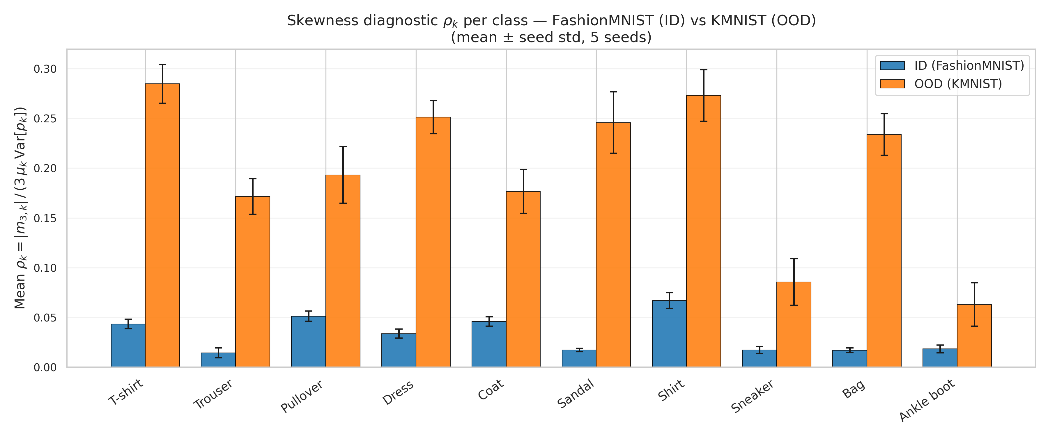
| Class | \(\bar\rho_k^{\text{ID}}\) | \(\sigma^{\text{ID}}\) | \(\bar\rho_k^{\text{OoD}}\) | \(\sigma^{\text{OoD}}\) | MWU \(p\) | OoD/ID |
|---|---|---|---|---|---|---|
| T-shirt/top | 0.04333 | 0.00476 | 0.28470 | 0.01950 | \(\approx 0\) | 6.57 |
| Trouser | 0.01426 | 0.00494 | 0.17139 | 0.01775 | \(\approx 0\) | 12.02 |
| Pullover | 0.05121 | 0.00506 | 0.19319 | 0.02847 | \(8 \times 10^{-260}\) | 3.77 |
| Dress | 0.03375 | 0.00451 | 0.25126 | 0.01659 | \(\approx 0\) | 7.45 |
| Coat | 0.04594 | 0.00462 | 0.17652 | 0.02213 | \(7 \times 10^{-264}\) | 3.84 |
| Sandal | 0.01726 | 0.00182 | 0.24578 | 0.03093 | \(\approx 0\) | 14.24 |
| Shirt | 0.06693 | 0.00777 | 0.27297 | 0.02592 | \(\approx 0\) | 4.08 |
| Sneaker | 0.01728 | 0.00344 | 0.08564 | 0.02328 | \(3 \times 10^{-56}\) | 4.96 |
| Bag | 0.01688 | 0.00236 | 0.23378 | 0.02085 | \(\approx 0\) | 13.85 |
| Ankle boot | 0.01832 | 0.00397 | 0.06293 | 0.02174 | \(5 \times 10^{-13}\) | 3.43 |
11.6.0.4 Interpretation.
These figures close the loop between Lemma 4 and the empirical OoD results. OoD inputs are not merely more uncertain (higher \(C_k\)) but more asymmetrically uncertain (higher \(\rho_k\)), at least for classes where the OoD population has meaningful predicted probability mass. When \(\rho_k \ll 1\) (ID regime), the second-order approximation is trustworthy and \(\sum_k C_k \approx \text{MI}\), so the two metrics converge. When \(\rho_k\) is large (OoD regime), the cubic correction in 38 becomes significant; \(\sum_k C_k\) captures this additional signal through its \(1/\mu_k\) weighting, while MI averages over the sampling distribution without per-class amplification. On FashionMNIST, where KMNIST induces consistently higher uncertainty across all ten logit outputs, the reversal is absent: every class shows \(\rho_k^{\text{OoD}} > \rho_k^{\text{ID}}\) (Figure 14).
11.7 Deep Ensemble OoD Detection: MIMIC-III↩︎
We repeat the MIMIC-III ICU\(\to\)Newborn OoD detection experiment using a deep ensemble of five members (one deterministic forward pass per member) in place of the low-rank Bayesian model. The ensemble uses the same 44-feature pipeline and identical evaluation code; uncertainty is derived from disagreement across members rather than MC sampling. As the ensemble consists of a single trained instance, no seed standard deviation is reported.
| Method | AUROC\(\uparrow\) | Ratio\(\uparrow\) |
|---|---|---|
| Neg.MSP | \(0.701\) | \(1.68\) |
| MI | \(0.752\) | \(2.32\) |
| \(EU_{\text{var}}\) | \(0.750\) | \(\mathbf{2.72}\) |
| \(\sum_k C_k\) | \(\mathbf{0.753}\) | \(2.31\) |
The ranking \(\sum_k C_k > \text{MI} > EU_{\text{var}}\) mirrors the low-rank Bayesian result (Table 1). Critically, \(EU_{\text{var}}\) again achieves the highest OoD/ID ratio (\(2.72\times\)) yet the lowest AUROC among epistemic measures: without mean-normalisation, boundary suppression compresses the dynamic range of scores, so a numerically large mean shift is swamped by within-group spread, failing to produce separable distributions. \(\sum_k C_k\) corrects this via the \(1/\mu_k\) weighting, yielding the highest AUROC across both inference regimes.
12 Epistemic Sensitivity to Data Quality: Supplementary Details↩︎
12.1 Model Architecture and Training↩︎
Both end-to-end models use low-rank Gaussian posteriors with the shared specification described in Appendix 11.2.
12.1.0.1 Fashion-MNIST.
Fully connected Bayesian network, two hidden layers of \(400\) units, rank \(15\), ReLU activations. Trained for \(50\) epochs with Adam (lr \(= 10^{-3}\)), batch size \(128\), \(S{=}50\) MC samples at inference.
12.1.0.2 CIFAR-10 (from scratch).
CNN with Conv \(32{\to}64{\to}128\), each followed by ReLU and \(2{\times}2\) max-pooling, global average pooling, and a low-rank Bayesian head (rank \(32\)). Trained for \(100\) epochs with Adam (lr \(= 10^{-3}\)), batch size \(128\), \(S{=}50\) MC samples at inference.
12.1.0.3 Label noise injection.
For each noise rate \(\alpha \in \{0.1, 0.2, 0.3, 0.4, 0.5\}\), a fraction \(\alpha\) of training labels is replaced uniformly at random across all classes. The test set remains clean throughout. Models are retrained from scratch at each noise level; results are mean over \(5\) seeds.
12.2 Transfer Learning Experiments↩︎
To isolate the effect of end-to-end Bayesian training, we repeat the disentanglement protocol with a frozen ImageNet-pretrained ResNet-50 backbone, replacing only the classifier head with one of three Bayesian variants:
Low-rank variational (rank \(= 32\), constrained posterior),
Full-rank variational (unconstrained Bayesian weight distributions),
MC Dropout (\(p{=}0.3\), deterministic weights with dropout-based uncertainty).
This design enables a controlled comparison: CIFAR-10 from scratch vs.CIFAR-10 transfer uses the same dataset, same \(K\), and same Bayesian model type (low-rank), isolating the training regime as the causal variable.
12.2.0.1 Why a relative ratio.
The naive absolute ratio \(R_{\mathrm{abs}}(\alpha) = (\bar{U}_e(\alpha) - \bar{U}_e(0))/(\bar{U}_a(\alpha) - \bar{U}_a(0))\) is confounded by the scale of epistemic uncertainty. Low-rank models produce baseline MI an order of magnitude below their full-rank counterparts (\(0.007\) vs.\(0.039\) on CIFAR-10; Table 22), so the absolute numerator \(\bar{U}_e(\alpha) - \bar{U}_e(0)\) is mechanically small regardless of whether the proportional increase is large or small. A low-rank model and a full-rank model with identical proportional epistemic leakage would report very different \(R_{\mathrm{abs}}\) values, making cross-model comparison misleading. The relative formulation \(R_{\mathrm{rel}}\) (Equation 13 ) normalises each delta by its own baseline, yielding a scale-invariant elasticity: for every \(1\%\) relative increase in aleatoric uncertainty, how many percent does epistemic uncertainty increase? This makes \(R_{\mathrm{rel}}\) directly comparable across models with different posterior families, rank constraints, and training regimes.
12.2.0.2 Baseline inflation.
Table 22 reports baseline epistemic uncertainty (\(\alpha{=}0\)) across all configurations. End-to-end models show negligible inflation of \(\sum_k C_k\) over MI (\(1.0\)–\(1.02\times\)), while transfer-learning models exhibit progressively higher inflation: low-rank (\(1.08\)–\(1.17\times\)), full-rank (\(1.35\)–\(1.59\times\)), MC dropout (\(1.62\)–\(1.89\times\)). Training regime matters more than dataset: CIFAR-10 low-rank with transfer learning (\(1.08\times\)) shows more inflation than CIFAR-10 low-rank from scratch (\(1.02\times\)) on the same data.
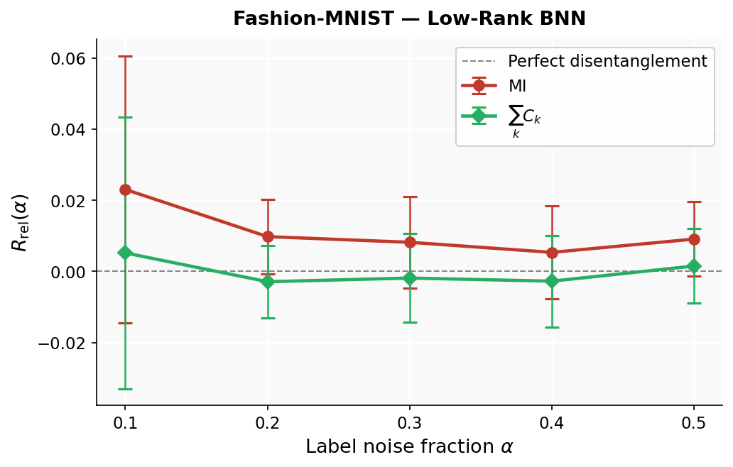

Figure 15: Disentanglement ratios \(|R_{\mathrm{rel}}(\alpha)|\) for end-to-end low-rank models. \(\sum_k C_k\) (green) is closer to zero than MI (red) at every noise level. Left: Fashion-MNIST. Right: CIFAR-10..
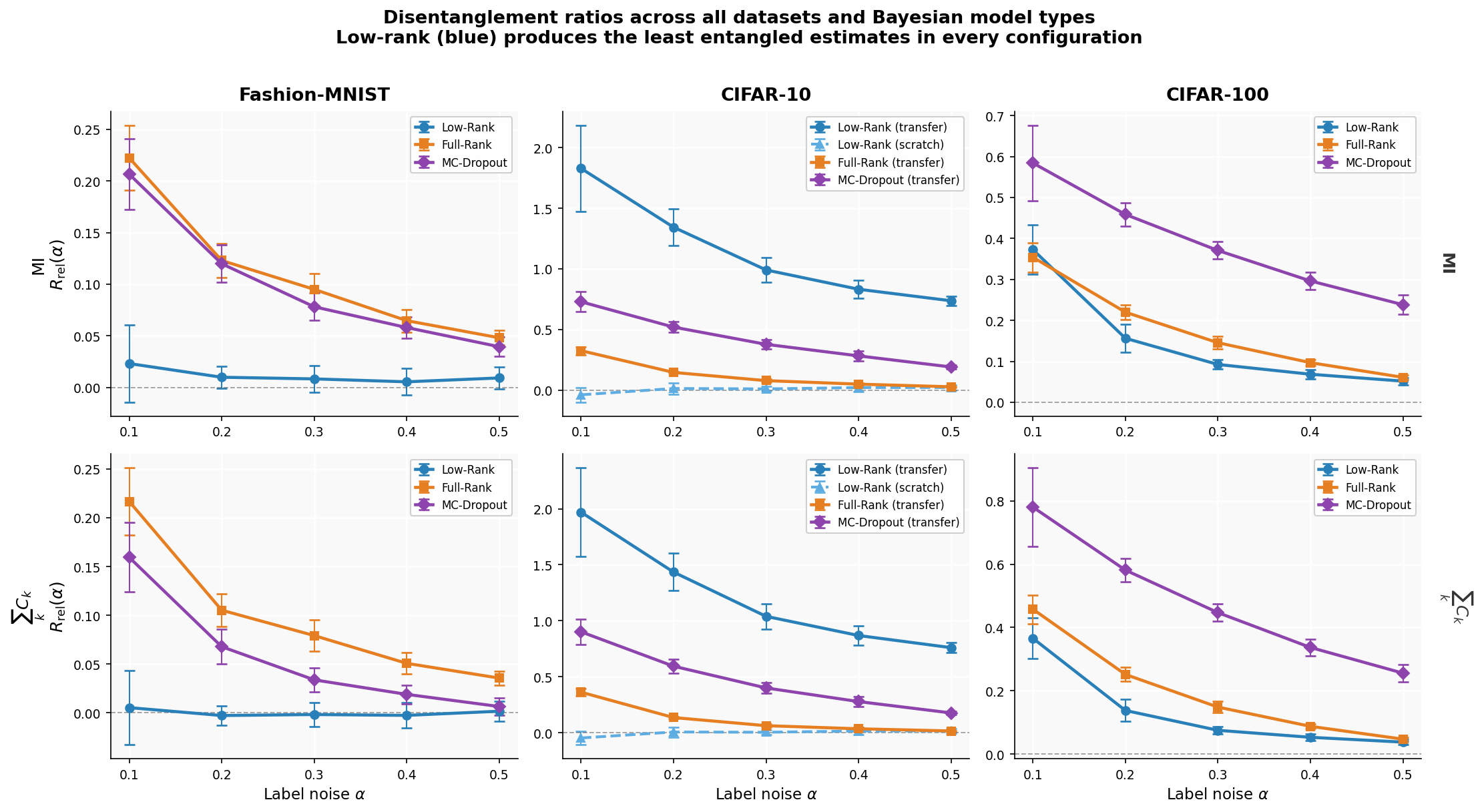
| Dataset | Model | Training | \(K\) | MI | \(\sum_k \Ck\) | Inflation |
|---|---|---|---|---|---|---|
| Fashion-MNIST | Low-rank Bayes | From scratch | 10 | 0.008 | 0.008 | \(1.00\times\) |
| CIFAR-10 | Low-rank Bayes | From scratch | 10 | 0.0067 | 0.0069 | \(1.02\times\) |
| CIFAR-10 | Low-rank Bayes | Transfer | 10 | 0.0045 | 0.0048 | \(1.08\times\) |
| CIFAR-10 | Full-rank Bayes | Transfer | 10 | 0.039 | 0.053 | \(1.35\times\) |
| CIFAR-10 | MC Dropout | Transfer | 10 | 0.039 | 0.063 | \(1.62\times\) |
| CIFAR-100 | Low-rank Bayes | Transfer | 100 | 0.042 | 0.049 | \(1.17\times\) |
| CIFAR-100 | Full-rank Bayes | Transfer | 100 | 0.190 | 0.302 | \(1.59\times\) |
| CIFAR-100 | MC Dropout | Transfer | 100 | 0.238 | 0.450 | \(1.89\times\) |
12.2.0.3 Disentanglement ratios: CIFAR-10 transfer.
Table 23 shows that under transfer learning MI outperforms \(\sum_k C_k\) for the low-rank model at all noise levels (\(|R_{\mathrm{rel}}| = 1.83\) vs.\(1.97\) at \(\alpha{=}0.1\)), consistent with the high inflation of this configuration. For full-rank models, \(\sum_k C_k\) overtakes MI at \(\alpha \geq 0.2\). MC dropout shows the worst overall ratios (\(0.18\)–\(0.90\)), with \(\sum_k C_k\) recovering at high noise (\(\alpha \geq 0.4\)). The model ordering for disentanglement quality is consistent: low-rank best under end-to-end training but worst under transfer, full-rank intermediate, MC dropout worst overall.
| Low-rank | Full-rank | MC Dropout | ||||
|---|---|---|---|---|---|---|
| 2-3 (lr)4-5 (lr)6-7 \(\alpha\) | MI | \(\sum_k \Ck\) | MI | \(\sum_k \Ck\) | MI | \(\sum_k \Ck\) |
| 0.1 | \(1.830\) | \(1.970\) | \(\mathbf{0.325}\) | \(0.362\) | \(0.728\) | \(0.901\) |
| 0.2 | \(1.344\) | \(1.435\) | \(\mathbf{0.145}\) | \(\mathbf{0.136}^{\dagger}\) | \(0.519\) | \(0.594\) |
| 0.3 | \(0.991\) | \(1.039\) | \(\mathbf{0.077}\) | \(\mathbf{0.063}^{\dagger}\) | \(0.377\) | \(0.400\) |
| 0.4 | \(0.832\) | \(0.868\) | \(\mathbf{0.048}\) | \(\mathbf{0.035}^{\dagger}\) | \(\mathbf{0.282}\) | \(\mathbf{0.278}^{\dagger}\) |
| 0.5 | \(0.737\) | \(0.760\) | \(\mathbf{0.026}\) | \(\mathbf{0.016}^{\dagger}\) | \(\mathbf{0.190}\) | \(\mathbf{0.177}^{\dagger}\) |
12.2.0.4 Disentanglement ratios: CIFAR-100 transfer.
Table 24 extends the analysis to \(K{=}100\). Low-rank achieves strong disentanglement (\(|R_{\mathrm{rel}}| < 0.37\)) for both metrics at all noise levels, with \(\sum_k C_k\) winning at every \(\alpha\). Full-rank shows MI winning at low noise but \(\sum_k C_k\) recovering at \(\alpha \geq 0.4\). MC dropout is the worst configuration: MI wins at all noise levels, with ratios exceeding \(0.58\).
| Low-rank | Full-rank | MC Dropout | ||||
|---|---|---|---|---|---|---|
| 2-3 (lr)4-5 (lr)6-7 \(\alpha\) | MI | \(\sum_k \Ck\) | MI | \(\sum_k \Ck\) | MI | \(\sum_k \Ck\) |
| 0.1 | \(0.373\) | \(\mathbf{0.366}^{\dagger}\) | \(0.354\) | \(0.458\) | \(0.584\) | \(0.780\) |
| 0.2 | \(\mathbf{0.156}\) | \(\mathbf{0.138}^{\dagger}\) | \(\mathbf{0.220}\) | \(\mathbf{0.252}\) | \(0.459\) | \(0.581\) |
| 0.3 | \(\mathbf{0.092}\) | \(\mathbf{0.075}^{\dagger}\) | \(\mathbf{0.145}\) | \(\mathbf{0.149}\) | \(0.371\) | \(0.447\) |
| 0.4 | \(\mathbf{0.069}\) | \(\mathbf{0.053}^{\dagger}\) | \(\mathbf{0.097}\) | \(\mathbf{0.088}^{\dagger}\) | \(\mathbf{0.296}\) | \(0.337\) |
| 0.5 | \(\mathbf{0.052}\) | \(\mathbf{0.038}^{\dagger}\) | \(\mathbf{0.061}\) | \(\mathbf{0.047}^{\dagger}\) | \(\mathbf{0.238}\) | \(\mathbf{0.256}\) |
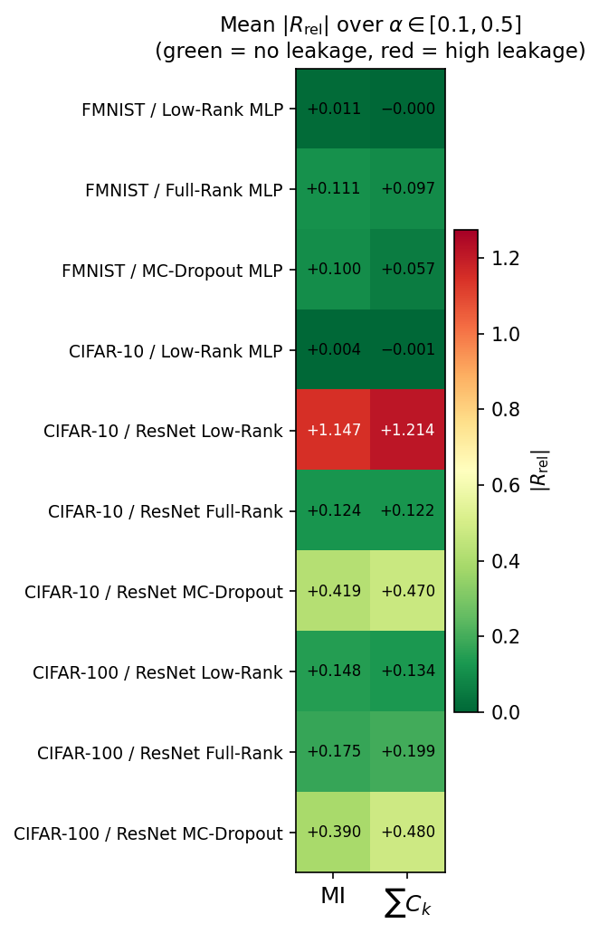
12.2.0.5 Key patterns across transfer-learning experiments.
The controlled comparison on CIFAR-10 is decisive: using the same dataset (\(K{=}10\)) and same model type (low-rank), training from scratch yields \(|R_{\mathrm{rel}}| < 0.05\) while transfer learning yields \(0.74\)–\(1.97\). This directly isolates the training regime as a causal factor. Within transfer learning, higher baseline inflation (\(\sum_k C_k\,/\,\text{MI}\)) correlates with worse \(\sum_k C_k\) performance relative to MI, a pattern that holds for both CIFAR-10 and CIFAR-100. The implication is that when the entire model participates in the Bayesian posterior, the resulting predictive distributions have a variance structure that is well captured by the \(C_k\) normalisation; when only a classifier head is Bayesian, this structure degrades.
12.2.0.6 Effect of rank constraint on uncertainty scale.
The low-rank variational framework of [25] parameterizes each weight matrix as \(W = AB^\top\) with independent mean-field Gaussian posteriors \(q(A)q(B)\) on the factors \(A \in \mathbb{R}^{m \times r}\), \(B \in \mathbb{R}^{n \times r}\). The induced posterior on \(W\) is singular with respect to Lebesgue measure, concentrating entirely on the manifold \(\mathcal{R}_r\) of rank-\(r\) matrices: every sampled weight matrix is constrained to have rank at most \(r\), though the specific column and row spaces vary across posterior samples. Under the same transfer-learning protocol on CIFAR-10, the low-rank model (\(r{=}32\)) produces baseline MI an order of magnitude below its full-rank counterpart (\(0.0045\) vs.\(0.039\)), a gap that persists across all noise levels (e.g., at \(\alpha{=}0.5\): \(0.047\) vs. \(0.072\)). The from-scratch low-rank model exhibits a similar absolute scale (\(\text{MI} = 0.0067\)), confirming that the compression is driven primarily by the rank constraint rather than the training regime. This compression has two distinct sources. First, the rank constraint itself restricts the number of independent directions along which weight matrices can vary; the resulting predictive distributions inherit this reduced dimensionality, yielding smaller \(\mathrm{Var}[p_k]\) and thus smaller MI. Second, while the factored posterior introduces structured correlations between weight entries (\(\mathrm{Cov}(W_{ij}, W_{i'j'}) \neq 0\) whenever the entries share latent factors), it remains mean-field within each factor, which is known to underestimate marginal variances relative to the true posterior [38], [39], further concentrating the predictive distribution. Crucially, this compression affects the absolute scale of uncertainty but not the relative ranking of inputs or the within-model metric comparison: since \(\sum_k C_k\) and MI share the same compressed scale by construction (Equation 8 ), their relative disentanglement ratios \(R_{\mathrm{rel}}(\alpha)\) remain directly comparable within a given model, and the finding that \(\sum_k C_k\) leaks less than MI holds independently of the overall scale. However, uncertainty thresholds calibrated on one posterior family cannot be transferred to another without recalibration, and the small absolute values produced by low-rank models should not be interpreted as evidence of low true epistemic uncertainty but rather as a consequence of both the manifold constraint on the posterior support and the mean-field under-dispersion within the learned factors.
12.3 Sensitivity to Class Cardinality↩︎
The \(1/\mu_k\) normalisation that corrects boundary suppression also introduces a scaling effect with the number of classes \(K\). Under the simplex constraint \(\sum_k \bar{p}_k = 1\), as \(K\) grows the average probability per class decreases. For a model assigning probability \(\alpha\) to the predicted class and distributing the remainder uniformly: \[\bar{p}_k \;=\; \frac{1-\alpha}{K-1} \quad \text{for } k \neq \text{pred}.\] Assuming approximately uniform variance \(\mathrm{Var}(p_k) \approx \sigma^2\) across classes: \[\sum_k C_k\;\approx\; \frac{\sigma^2}{2\alpha} \;+\; \frac{(K-1)^2\,\sigma^2}{2(1-\alpha)} \;\sim\; \mathcal{O}(K^2),\] whereas MI, measuring entropy differences bounded by \(\log K\), does not accumulate linearly over classes.
Empirically, this manifests as higher baseline inflation on CIFAR-100 compared to CIFAR-10 for every model type (Table 22): low-rank \(1.17\times\) vs.\(1.08\times\); full-rank \(1.59\times\) vs.\(1.35\times\); MC dropout \(1.89\times\) vs.\(1.62\times\). The \(K\)-dependence interacts with model type: low-rank models remain resilient at \(K{=}100\) (\(|R_{\mathrm{rel}}| < 0.37\)), while MC dropout fails substantially (\(|R_{\mathrm{rel}}|\) up to \(0.78\) at \(\alpha{=}0.1\)).
12.3.0.1 Mitigation strategies.
For high-cardinality settings (\(K \gtrsim 50\)), two modifications can reduce inflation without sacrificing the per-class interpretability of \(C_k\): (i) truncated summation, restricting \(\sum_k C_k\) to the top-\(k\) most probable classes, which eliminates the accumulation of amplified terms from negligible-probability classes; (ii) probability-weighted aggregation, weighting each \(C_k\) by \(\mu_k\) to down-weight low-probability contributions. We recommend reporting both \(\sum_k C_k\) and MI in high-\(K\) settings: the per-class decomposition retains interpretive value even when the aggregate \(\sum_k C_k\) underperforms MI as a scalar summary.
References↩︎
Concurrently, [16] show that pretrained deep ensembles exhibit worse AU/EU disentanglement than models trained from scratch, a conclusion we reach independently in Section 5 via both the degradation of the \(C_k\) approximation and increased AU/EU entanglement under transfer learning.↩︎
[14] also exploit a Taylor expansion to relate softmax variance to MI, but expand the logarithm \(\log p_k\) rather than the entropy function \(H(\boldsymbol{p})\) itself (their Section 3.2, Eq. 10). This yields a class-averaged variance \(\frac{1}{K}\sum_k\mathrm{Var}[p_k]\) with equal weights per class, whereas expanding the entropy via its Hessian yields the curvature-weighted sum \(\frac{1}{2}\sum_k\mathrm{Var}[p_k]/\mu_k\), in which the \(1/\mu_k\) factor enables per-class attribution.↩︎
The ratio \(\mathrm{Var}[p_k]/\mu_k\) coincides with the index of dispersion [17] (Fano factor [18]). Here the \(\tfrac{1}{2}\) prefactor and the \(1/\mu_k\) weighting both emerge from the entropy Taylor expansion, so the components sum to a well-defined information-theoretic quantity.↩︎
We also evaluated a binary cross-boundary MI variant (MI computed on the binary safe-vs-critical partition), which achieves AUSC \(0.284 \pm 0.015\), essentially tied with \(C_{\text{crit\_max}}\) (mutual win rate 49.5%/50.5%). It is excluded from the main comparison because it is not part of the \(C_k\) framework and exhibits numerical instability (\(\texttt{NaN}\) values when \(\mu_{\text{safe}} \approx 0\) or \(\mu_{\text{safe}} \approx 1\)).↩︎