Quasars behind the disk of M 31 galaxy
February 23, 2026
We aim to increase the limited number of quasars behind M 31, necessary for probing the chemical content of the gas and for proper motion reference, with reliable and homogeneous redshift measurements from emission lines. We carried out spectroscopic follow up of 32 quasar candidates. We confirm 23 quasars: two are new discoveries (J004029.727+403705.68 and J004215.489+412031.52) and the rest were reported elsewhere, but with somewhat deficient analysis; 16 spectra are published for the first time. We report new homogeneous redshifts for 34 quasars (from 40 spectra, adding 17 from archives) and summarize all available information about bona-fide quasars with reliable redshift, bringing their number to 124 within the \(\mu_B\)=26\(^m\)/\(\Box\arcsec\) isophote. We carried out a comparison of redshifts from different sources and excluded some objects with redshifts derived from low-resolution spectra. We derive the reddening for them from the color excess with respect to dereddened counterparts with similar redshifts in the field. Comparisons of our reddenings with M 31 reddening maps found no significant correlations. Most QSOs behind M 31 show low reddening and do not probe high-extinctions underlining the need to identify fainter quasars behind nearby galaxies, especially behind higher extinction regions – probably due to a bias towards following up brighter and less extinct candidates. Finally, the redshifts derived from low-resolution spectra must be treated with caution, because they can contain significant errors.
Quasars behind M 31
1 Introduction↩︎
Quasars behind nearby galaxies are of great value for probing their kinematics and interstellar medium. They establish a non-moving reference system for astrometric studies [1]–[3]. The quasars are background sources that allow to study the extinction in the intervening absorbers that can be both nearby low-redshift galaxies or distant high-redshift objects [4]–[6]. The imprinted narrow absorption features from the interstellar material (ISM) on the quasar spectra can be used to measure the chemical composition and the velocity field of the ISM [7]–[11]. These observations, carried out in the UV, where the strong absorption features of the cold interstellar gas are, allow to trace the chemical enrichment history of the intervening galaxies, and to trace the origin of the extended gaseous structures, such as the Magellanic stream, to a particular galaxy, in this case – to the Small Magellanic cloud. UV bright quasars are necessary for such studies and they are usually found from surveys in the region such as GALEX [12], but they are relatively rare and only a few exist behind the nearest galaxies.
The mere identification of quasars is a challenge on its own. Usually, it is based on their optical colors [13], variability properties [14], [15], or their X-ray, UV or mid-infrared (mid-IR) emission [16], [17], [18] among others. The presence of a galaxy in front of the quasar introduces additional complications – contamination from foreground sources that in the general case can be variable, e.g. seeing dependent or due to the intrinsic variability of the contaminating source. However, these problems are solvable, for example, with a combination of some of these methods: [19] and [20], [21] easily reached a success rate of \(>\)70% despite the contamination from the Magellanic clouds, selecting quasar candidates from near-infrared (near-IR) colors and variability. They defined a locus of previously known quasars on the \(J\) \(-\) \(K_S\) vs \(Y\) \(-\) \(J\) color-color diagram with photometry from the VISTA Magellanic Survey [22] and followed up spectroscopically objects located inside this region. Its borders were adjusted to reduce the contamination, mostly from evolved stars. This is acceptable as long as the goal of the search is to efficiently identify quasars, but not necessarily to obtain a complete sample. Next, they took advantage of the time-series data from the VMC survey to identify the most variable objects by parameterizing the light curves with a simple linear fit and required a minimum absolute slope value. M 31 and M 33 present a greater challenge than the Magellanic system due to the higher surface stellar density, the worse contamination by objects in the more crowded intervening galaxies and because of the generally higher extinction, except for the inner SMC region.
Here we report the confirmation of 23 quasar candidates behind the M 31 disk with spectra (resolution 700\(\le\) \(\lambda\)/\(\Delta\lambda\) \(\le\)1100). Two of them are completely new discoveries, and the other 21 spectra confirm the quasar nature of previously announced candidates. We also uniformly measured redshifts for 34 unique quasars from 40 spectra – adding 17 archival to our data. Summarizing, we built a list of 125 spectroscopically confirmed QSOs within the \(\mu_B\)=26\(^m\)/\(\Box\arcsec\) isophote (Sec. 2).
The next two sections describe out target selection and the observations. Section 4 presents the analysis of the spectra, Section 5 is an extinction study and 6 gives a summary.
2 Target selection↩︎
M 31 and M 33 present a greater challenge than the Magellanic clouds due to the higher surface stellar density. The census of the quasars behind any galactic disk depends on its adopted boundaries. For example, [23] list 8 previously known and 7 newly found QSOs1 within the footprint of M 31 Local Group Galaxy Survey [24]. Three more QSO, known at the time, were missing in this list: one reported by [25] and two others – by [26], bringing the total number of the known QSOs within this survey up to 18.
However, the LGSS is designed to cover the region of active star formation, especially the eastern side that is further from the Milky Way; the M 31’s disk extends further outside the survey’s footprint. To compensate for this offset, we adopt here a wider and physically defined area of interest adopting as a galaxy limit the ellipse with a major diameter D26=225\(\arcmin\), corresponding to the surface brightness level \(\mu_B\)=26\(^m\)/\(\Box\arcsec\) of [27]. We adopt a position angle PA=35 deg and major-to-minor diameters ratio of 3.09 that RC3 [Third Reference Catalog of Bright Galaxies; [28]] reports for the somewhat brighter, but better defined standard isophote of \(\mu_B\)=25\(^m\)/\(\Box\arcsec\). For the center of M 31, we adopt the coordinates as determined in 2MASS [29]: \(\alpha\)=0:42:44.33 \(\delta\)=+41:16:07.5 (J2000).
Our ellipse encompasses well all footprints of the modern catalogs with IR and optical photometry in M 31, as well as the dust maps available in the literature.
We found spectra of 6 candidates, in addition to the previously known 18 quasars within the selected area. Four of these extra spectra were observed by LAMOST (Large Sky Area Multi-Object Fibre Spectroscopic Telescope) as a part of its Quasar Survey 2012-2017 [26], [30] and are publicly available in LAMOST DR52. Other 2 QSOs are reported by [25]. Interestingly, the latest LAMOST Quasar Survey DR6-DR9 2017-2021 [31] does not report any QSOs behind the M 31 disk.
![Figure 1: Map of the 24 bona-fide QSOs (red squares) with prominent emission lines and 1 BL Lac object (red dot) known from the literature before Gaia DR3 [32]. The confirmed QSOs from our target list are also shown: 3 Spitzer-selected (cyan), 2 selected from optical colors and UV excess (yellow) and 18 selected by other means (see Table 1; black). All objects are located within the \mu_B=26^m/\Box\arcsec isophote (black solid line). The \mu_B=25^m/\Box\arcsec isophote (dotted line), the approximate boundaries of the Spitzer PSC catalog (dashed line) and the footprints of LGGS (red) and PHAT (blue) catalogs are also plotted.](/article/2602.20318/qso_before_GDR3.png "fig:")
In total, there are 25 objects with spectroscopically derived optical redshifts within the D26 ellipse: 24 bona-fide QSOs with prominent emission lines and a BL Lac discovered by [33]. Their positions are shown in Fig. 1, together with D26 and D25 isophotes and the footprints of M 31 photometric catalogs: [24], [34] and [35].
Recently, Gaia DR3 contributed to the global census of QSOs adding 6.4 million sources classified as AGN [36]. The extragalactic catalog of Gaia DR3 [32] reports parameters derived from various post-processing modules dedicated to the classification and characterization of more than 6.64 million objects considered as QSO candidates but only 159 quasar candidates behind the M 31 disk are classified as AGN. Among them 120 have derived redshifts based on the spacecraft’s spectrograph with a resolving power R\(\sim\)30-100. However, a careful comparison with better quality data from the literature, including our own measurements reported here, suggested that about 30% of these redshifts are significantly different from measurements that we deem more reliable. This broadly agrees with their own assessment that \(\sim\)36% of the quasars have redshift errors \(>\)0.1 dex, and of Quaia survey3 that finds an even higher fraction of \(\sim\)47% (if the warning flags are ignored). Therefore, we omitted from our analysis these Gaia redshifts. Objects included in this list are still considered, if other sources reported redshifts, and those other redshifts were used.
[37] listed 184 “quasars behind the disk of M 31” from spectroscopy with Dark Energy Spectroscopic Instrument [38] but only 14 of them are located within D26 ellipse. They are by-product of comprehensive spectral survey (resolution 2000\(\le\) \(\lambda\)/\(\Delta\lambda\) \(\le\)5500) of 11,416 objects on the Mayall 4m telescope at KPNO in two fields with \(3.\!\!{^\circ}2\) diameter, one centered on M 31 itself and the other to the South of it. The selection criteria involve negligible parallaxes and proper motions and combine Gaia DR2 and unWise photometry [39], [40]. They do not list errors but 51 of their quasars–many located far outside the disk of M 31–have redshifts in [41], [42], [25], [30], [23], and [26]. Their object No. 141 with \(z\)=1.778 is classified based on the LAMOST spectrum as a star at the velocity of M 31, and for their object No. 39 the LAMOST redshift is 1.600, as opposed to their 2.956; for the remaining objects the mean redshift difference is 0.004\(\pm\)0.016 and we consider this a reliable source of confirmed quasars.
[43] revisited the Gaia spectra, also combining them with unWISE colors. They implemented cuts based on proper motions and colors, thereby reducing the number of contaminants by approximately fourfold. They used machine learning to improve the Gaia redshift estimates. Although based on the same low-resolution Gaia spectra, the number of catastrophic outliers were reduced by a factor of 3 with respect to the unvetted analysis; 91% of their redshifts agree with the SDSS DR16 measurements [44] to within 0.2 dex. The final catalog contains 1,295,502 quasars with G\(<\)20.5 mag, and 755,850 candidate objects in an even cleaner G\(<\)20.0 mag sample. They reported 105 QSOs within the M 31 disk. Their counterparts in Gaia DR3 which have a Class AGN are 54 and the remaining 50 are not classified.
Our data and the literature reports produce a sample of 124 unique bona-fide spectroscopically confirmed quasars and 1 BL Lac within the \(\mu_B\)=26\(^m\)/\(\Box\arcsec\) isophote.
The sample selection is heterogeneous, because of the non-uniform coverage of different surveys that provided the photometric data. Therefore, it is difficult to estimate the selection bias and completeness of our search (see Sect. 4.2).
Thirteen spectra came from a campaign to confirm optical and X-ray selected high mass binaries in M 31 [45]; 12 of them were identified as quasars and one was a M star (No. 14 in Table 1).
Next, we expanded our search to the mid-IR. Initially, its footprint was limited to the Panchromatic Hubble Andromeda Treasury survey [34] where deep and high angular resolution imaging allowed to identify isolated bright candidates that meet the mid-IR criteria of [46], based on colors from the Wide-field Infrared Survey Explorer [47]. This is shown in Fig. 2 (top panel). We obtained spectra of 4 candidates from this selection.
We further expanded the target selection to include the Local Group Galaxy survey [24] combining it with mid-IR Spitzer photometry of [35]. Following [46], we defined a locus (Fig. 2, middle) of known quasars in the Spitzer colors space as follows: \[\label{eq:MIR95selection} \begin{array}{l} ([3.6]-[4.5])\geq-3.17\times([4.5]-[8.0])+4.75\\ ([3.6]-[4.5])\geq0.6\times([4.5]-[8.0])-0.90\\ ([3.6]-[4.5])\leq0.6\times([4.5]-[8.0])-0.05 \end{array}\tag{1}\]
This is an intentionally conservative definition that excludes some known quasars, but it helps to reduce the contamination by red stars. In addition, we required that ([4.5]\(-\)[24])\(\geq\)4.5 mag and that the sources are isolated – the degree of crowding index defined by [24] is \(<\)5%. Nineteen (\(\sim\)85%) of the 22 known quasars fall within the locus defined by these criteria; the three remaining sources are nearby AGNs where the nuclei may be contaminated by the emission from the galaxy disks (Fig. 2, bottom). Even these conservative criteria yielded hundreds of potential QSOs, but only a handful of them were bright enough in the optical for follow up spectroscopy: 10 have \(R\) \(\leq\)19.2 mag, 32 with 19.2\(<\) \(R\) \(\leq\)20.0 mag, and 62 with 20.0\(<\) \(R\) \(\leq\)20.5 mag, giving us in total 104 LGGS objects within a searching radius of 1.5\(\arcsec\). We obtained spectra of only 8 of these.
Seven quasars from Yuhan Yao4 were reidentified among known X-ray [48] and reobserved producing homogeneous redshifts for 6 of them. The remaining object (No. 4 in Table 1) was classified as an X-ray binary.
The complete list of 32 observed candidates is given in Table 1. In the process of matching the optical and mid-IR surveys, we discovered some systematic differences in the coordinates of [35]. The applied corrections with respect to WISE catalog are described in Appendix 9.
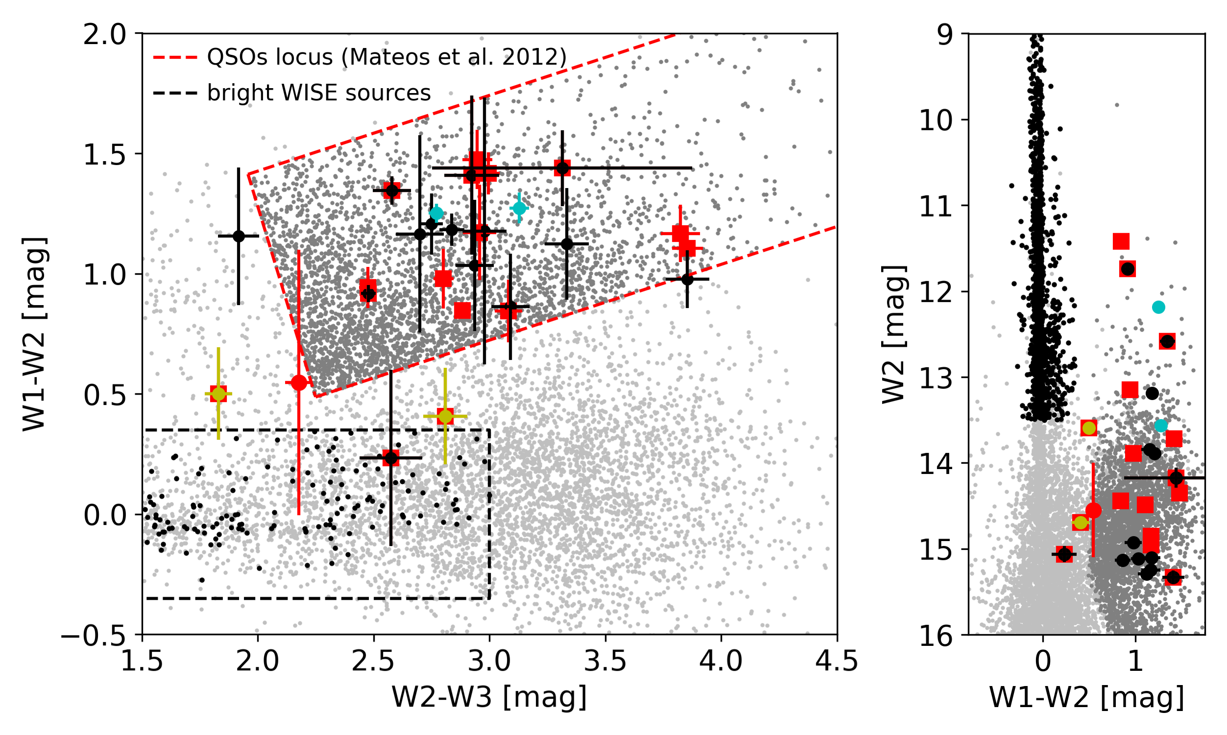
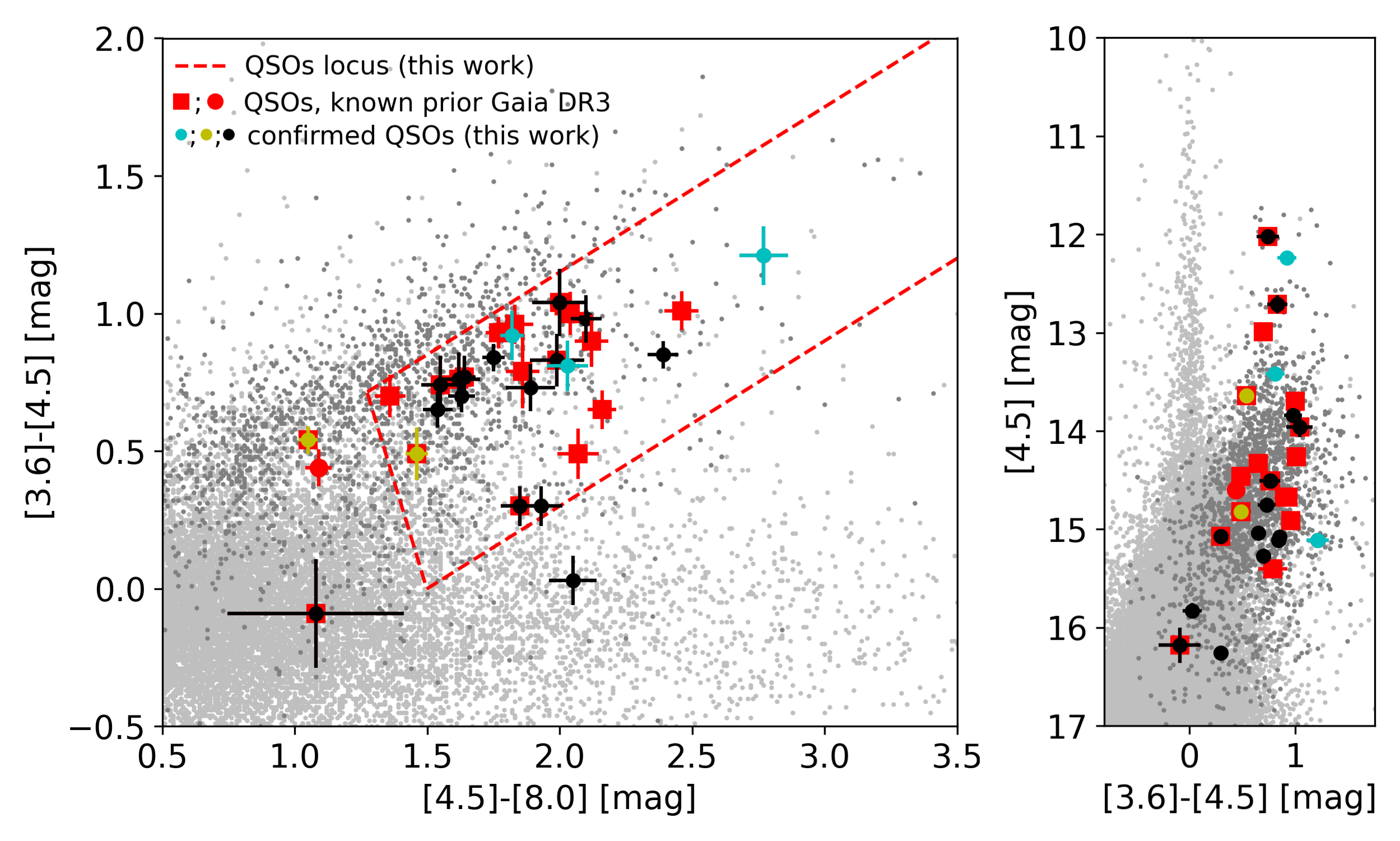
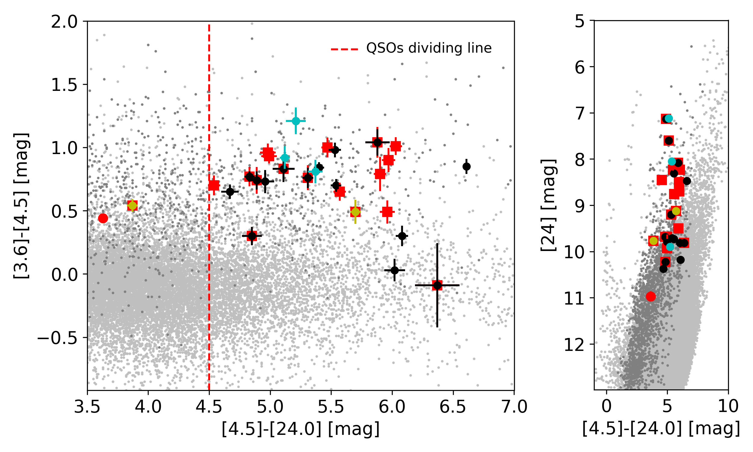
Figure 2: Illustration of our MIR color selection (see Sec. 2 for details). Top: WISE color–color (left) and color-magnitude diagram (right). The symbols in all panels are the same as in Fig. 1. Small gray dots show the entire WISE photometry within the Spitzer footprint. Small black solid dots are the sample of bright WISE sources used to adjust the coordinates (see Appx. 9 for details). The red dashed lines show our adopted quasar locus defined in Eqs. 1 after [46]. The sources falling inside are plotted with dark gray in all panels. Middle and bottom: Similar diagrams, but with Spitzer 3.6, 4.6 and 8 or 24 \(\mu\)m bands. The dashed vertical line in the bottom plot shows our additional color constraint. Summarizing, our targets for follow up spectroscopy were selected among dark gray points that meet this additional criterion..
3 Observations and data reduction↩︎
The spectroscopic confirmation was obtained by low-resolution optical spectroscopy that allows to recognize quasars from the broad emission lines in their spectra. Part of the spectra were obtained with the Dual Imaging Spectrograph5 (DIS) at the 3.5m telescope at the Apache Point Observatory (marked with A in column Telescope in Table 1), with the B400 and R300 gratings in the blue (\(\lambda\) \(\approx\)3425–5900 Å) and red (\(\lambda\) \(\approx\)5180–9860 Å) channel, respectively. The 1.5 arcsec slit was used, delivering resolving power of R\(\approx\)700 and 850 at the centers of the wavelength ranges for the blue and red arms, respectively.
The remaining spectra were obtained at the 6m telescope at the Special Astrophysical Observatory (SAO) of the Russian Academy of Sciences (marked with B in column Telescope in Table 1) with SCORPIO-16 [grisms VPHG1200B and VPHG1200R, spectral ranges and resolutions are \(\lambda\) \(\approx\)3600–5400 Åand R\(\approx\)800, \(\lambda\) \(\approx\)5700–7400 ÅR\(\approx\)1300, respectively; 1.2 arcsec wide slit; [49]] and SCORPIO-27 [grism VPHG1200@540, spectral range \(\lambda\) \(\approx\)3650–7250 Å, resolution R\(\approx\)1000; 1.0 arcsec wide slit; [50]]. Table 1 shows the log of our observations.
| No | Gaia | RA DEC | G, | Tel. | UT start | N\(_{\rm exp}\)\(\times\) | No. in | Selection criteria; comments |
| EDR3 | (J2000) | mag | 20yy-mm-dd | int. | Table | |||
| Thh:mm | time, s | |||||||
| 1* | 381231021002898048 | 00:39:21.921 41:20:31.31 | 20.52 | B | 21-11-03T21:18 | 6\(\times\)900 | 15 | Opt. colors & PTF variability |
| 2* | 381230200663395712 | 00:39:28.105 41:19:13.09 | 20.77 | B | 21-11-03T23:04 | 4\(\times\)900 | 16 | Opt. colors & PTF variability |
| 3* | 381223637953333376 | 00:39:34.595 41:07:38.52 | 19.88 | B | 21-11-04T19:34 | 3\(\times\)900 | 18 | Opt. colors & PTF variability |
| 4* | 381251297542795904 | 00:39:47.423 41:31:47.53 | 20.31 | B | 21-10-12T17:17 | 3\(\times\)900 | 21 | Opt. colors & PTF variability |
| 5 | 156600101021498792\(^a\) | 00:40:24.514 40:30:25.12 | 20.00\(^a\) | B | 21-12-12T20:37 | 8\(\times\)600 | Opt. colors & PTF variability; not QSO, X-ray binary? | |
| 6* | 381129011231416704 | 00:40:29.727 40:37:05.68 | 18.98 | A | 07-11-03T01:34 | 3\(\times\)2700 | 27 | X-ray & LGGS |
| A | 07-11-09T02:07 | 3\(\times\)2700 | ||||||
| 7 | 381159003004920192 | 00:40:45.721 40:51:34.18 | 19.24 | A | 20-01-02T04:55 | 2\(\times\)1800 | Spitzer colors & LGGS; too low S/N to interpret | |
| 8 | 381161584267072896 | 00:41:26.217 40:53:26.55 | 19.95 | A | 07-10-10T04:38 | 3\(\times\)2700 | 41 | X-ray & LGGS |
| 9 | 381164710999391104 | 00:41:37.918 41:01:07.82 | 19.40 | A | 07-08-10T08:55 | 4\(\times\)1800 | 45 | X-ray & LGGS |
| 10 | 381276410213544064 | 00:41:41.408 41:19:16.85 | 18.57 | A | 07-10-09T02:05 | 3\(\times\)2700 | 46 | X-ray & LGGS |
| 11* | 381266244030810880 | 00:42:15.487 41:20:31.52 | 20.54 | A | 10-10-30T02:46 | 6\(\times\)2700 | 57 | X-ray & LGGS |
| 12* | 369148728241389056 | 00:42:35.002 40:48:39.20 | 18.81 | A | 07-08-11T10:55 | 3\(\times\)1200 | 62 | X-ray & LGGS |
| A | 10-10-30T01:34 | 3\(\times\)1500 | ||||||
| 13 | 369257652908605824 | 00:43:12.746 41:16:25.49 | 18.58 | A | 18-10-07T02:27 | 2\(\times\)1800 | UV excess in LGGS & PHAT; not QSO, star forming region or galaxy? | |
| 14 | 369255522604831232 | 00:43:53.335 41:16:55.90 | 19.51 | A | 07-08-08T07:59 | 2\(\times\)1800 | X-ray & LGGS; not QSO, early M star | |
| 15 | 369286102772174208 | 00:44:10.843 41:33:01.15 | 19.22 | A | 19-01-08T05:16 | 2\(\times\)1500, | Spitzer colors & LGGS; flat feature- | |
| A | 1\(\times\)602 | less spectrum | ||||||
| 16 | 369281288111420288 | 00:44:28.716 41:25:45.62 | 18.96 | A | 19-01-06T04:03 | 2\(\times\)1500, | Spitzer colors & LGGS; not quasar, | |
| A | 1\(\times\)1034 | K-type star or globular cluster, at the redshift of M 31 | ||||||
| A | 19-01-08T04:17 | 2\(\times\)1200 | ||||||
| A | 19-09-05T08:25 | 3\(\times\)1500 | ||||||
| B | 22-10-25T17:33 | 3\(\times\)900 B | ||||||
| B | 22-10-25T18:25 | 2\(\times\)900 R | ||||||
| 17 | 369281086247278080 | 00:44:31.624 41:24:10.69 | 19.86 | A | 19-10-27T03:35 | 6\(\times\)1800 | Spitzer colors & LGGS; not quasar, wide emission lines object | |
| 18* | 369185428738695808 | 00:44:41.590 40:46:43.46 | 19.10 | B | 21-10-02T22:11 | 3\(\times\)900 B | 79 | Opt. colors & PTF variability |
| B | 21-10-02T22:59 | 2\(\times\)900 R | ||||||
| 19 | 381304653920639488 | 00:44:45.117 41:47:20.52 | 19.31 | A | 19-10-27T01:13 | 4\(\times\)1800 | Spitzer colors + LGGS; too low S/N to interpret | |
| 20* | 369267681654714112 | 00:44:48.307 41:16:18.23 | 18.43 | A | 19-01-06T01:57 | 3\(\times\)900 | 82 | Spitzer colors + LGGS |
| A | 20-01-02T01:57 | 2\(\times\)1800 | ||||||
| 21* | 369189547608980224 | 00:44:57.601 40:59:13.85 | 20.47 | B | 21-12-11T15:20 | 4\(\times\)600 | 83 | Opt. colors & PTF variability |
| 22* | 369268712447126272 | 00:44:57.938 41:23:43.72 | 19.67 | A | 07-11-09T03:45 | 2\(\times\)1800 | 84 | X-ray & LGGS |
| 23 | 369288714109887744 | 00:45:27.311 41:32:54.06 | 20.39 | A | 18-10-07T08:03 | 4\(\times\)1800 | 92 | UV excess in LGGS & PHAT |
| 24* | 369276756923364224 | 00:45:28.249 41:29:43.92 | 19.53 | A | 18-10-07T05:08 | 4\(\times\)1800 | 93 | UV excess in LGGS & PHAT |
| 25 | 369270469091280000 | 00:45:43.426 41:20:30.86 | 19.27 | A | 07-07-16T08:29 | 3\(\times\)1800 B | 95 | X-ray & LGGS |
| A | 4\(\times\)1500 R | |||||||
| 26 | 375332454650675328 | 00:46:32.809 42:13:14.25 | 19.10 | A | 18-10-07T04:06 | 3\(\times\)900 | UV excess in LGGS & PHAT; featureless spectra, no emission lines | |
| 27 | 375328709439174400 | 00:46:55.515 42:20:50.09 | 17.65 | A | 10-10-30T05:12 | 3\(\times\)900 | 108 | X-ray & LGGS |
| 28* | 375328395906539392 | 00:47:02.870 42:18:37.19 | 19.90 | A | 10-10-10T07:37 | 8\(\times\)836 | 109 | X-ray & LGGS |
| 29* | 375328876942905472 | 00:47:13.476 42:20:47.66 | 19.92 | A | 07-07-24T08:05 | 4\(\times\)1800 | 111 | X-ray & LGGS |
| 30* | 375423881617811328 | 00:47:39.120 42:26:17.76 | 18.20 | A | 19-01-06T02:54 | 3\(\times\)1200 | 115 | Spitzer colors & LGGS |
| 31 | 375322314232658048 | 00:47:42.847 42:10:16.93 | 19.74 | A | 08-10-26T01:29 | 3\(\times\)2700 | 116 | X-ray & LGGS |
| 32* | 375418590218050304 | 00:47:48.323 42:19:34.31 | 19.13 | A | 19-01-08T03:07 | 3\(\times\)1200 | 118 | Spitzer colors & LGGS |
| A | 20-01-02T03:10 | 3\(\times\)1800 |
The data were reduced with Image Reduction and Analysis Facility8 [53], [54] and ESO Munich Image Data Analysis System9 [55], [56]. The usual steps for long slit data processing were performed: bias/dark subtraction, flat fielding and wavelength calibration. The 1-dimensional spectra were extracted within 0.8–1.2 arcsec wide apertures, approximately matching the seeing during the observations for the DIS data, or using the optimal extraction code SPEXTRA, specifically designed for crowded fields [57], for the SCORPIO data. The spectra were flux calibrated with spectrophotometric standards from [58] and [59], [60], but given the non-photometric conditions during most of the observations, it is relative, so we only recovered the correct shape of the spectra, not their absolute flux. The quasar spectra are plotted in Fig. 3.
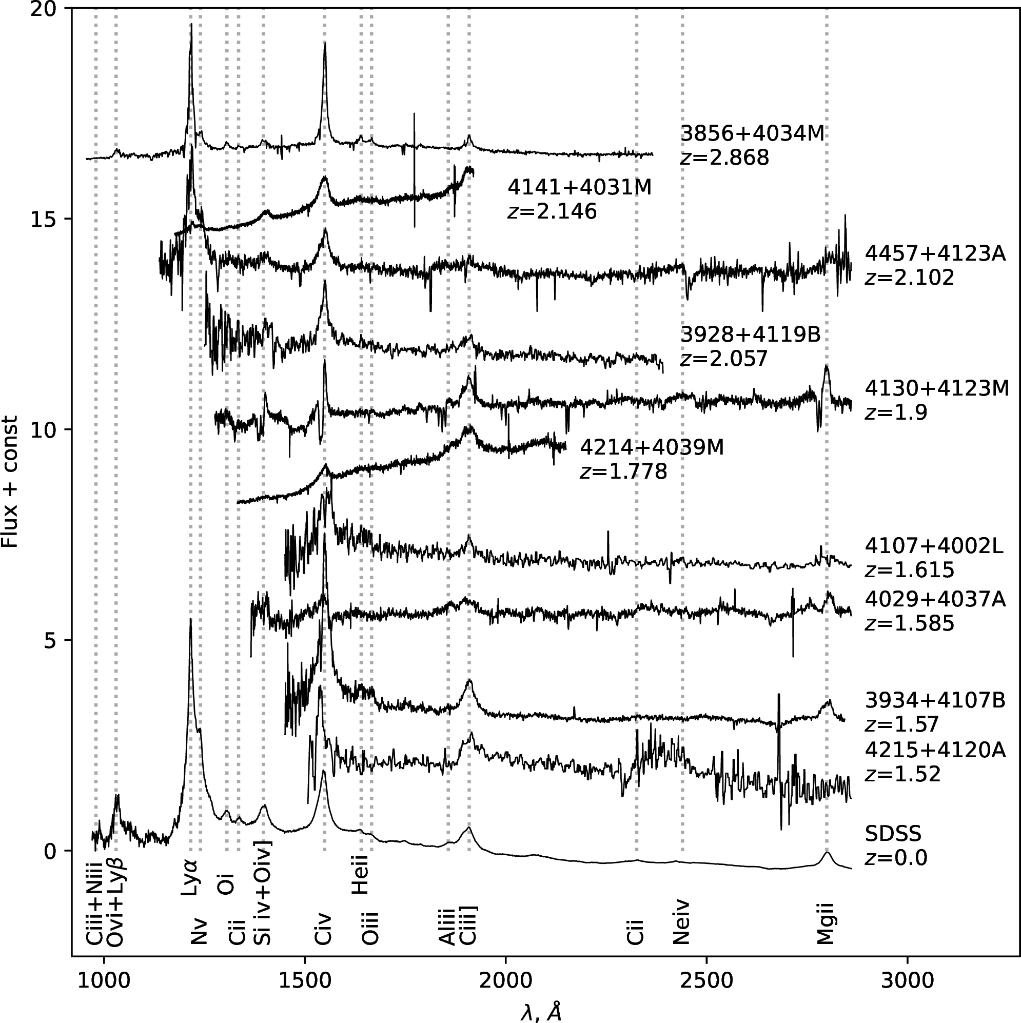
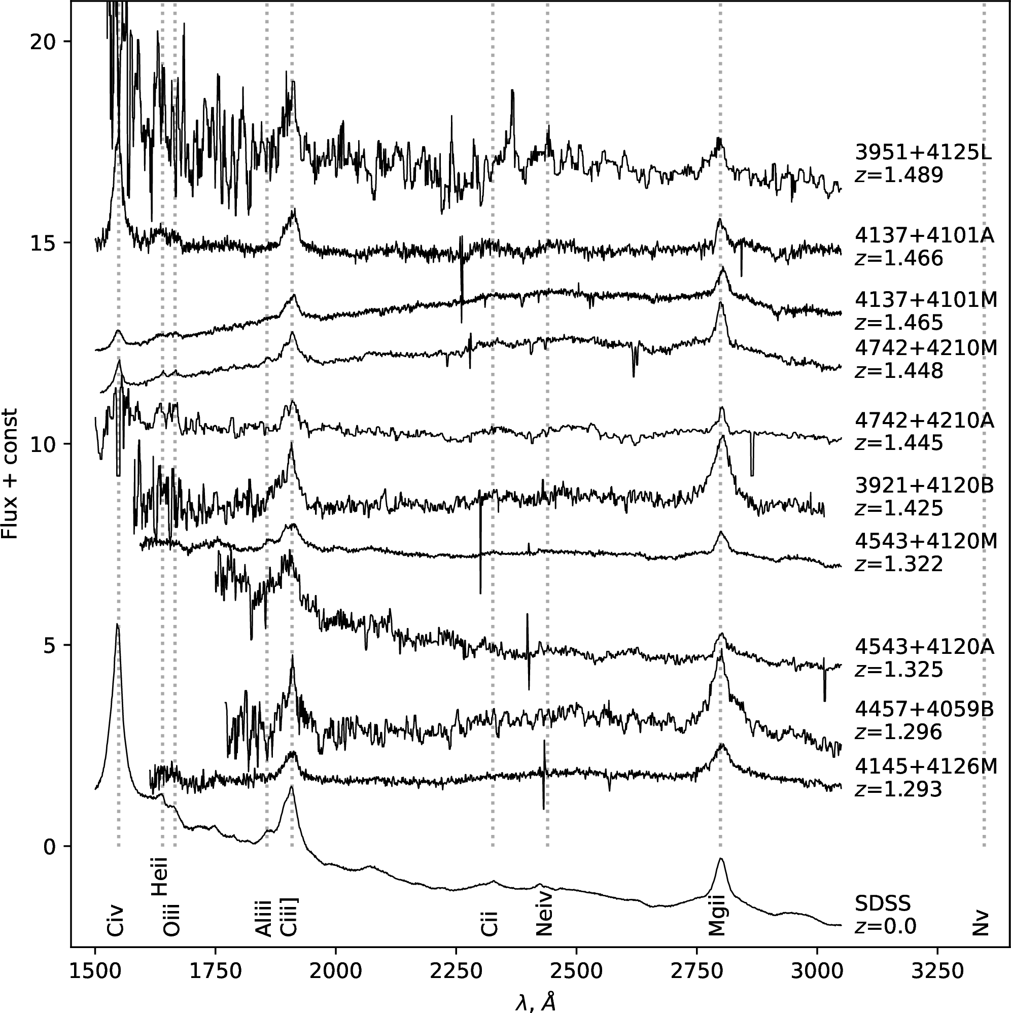
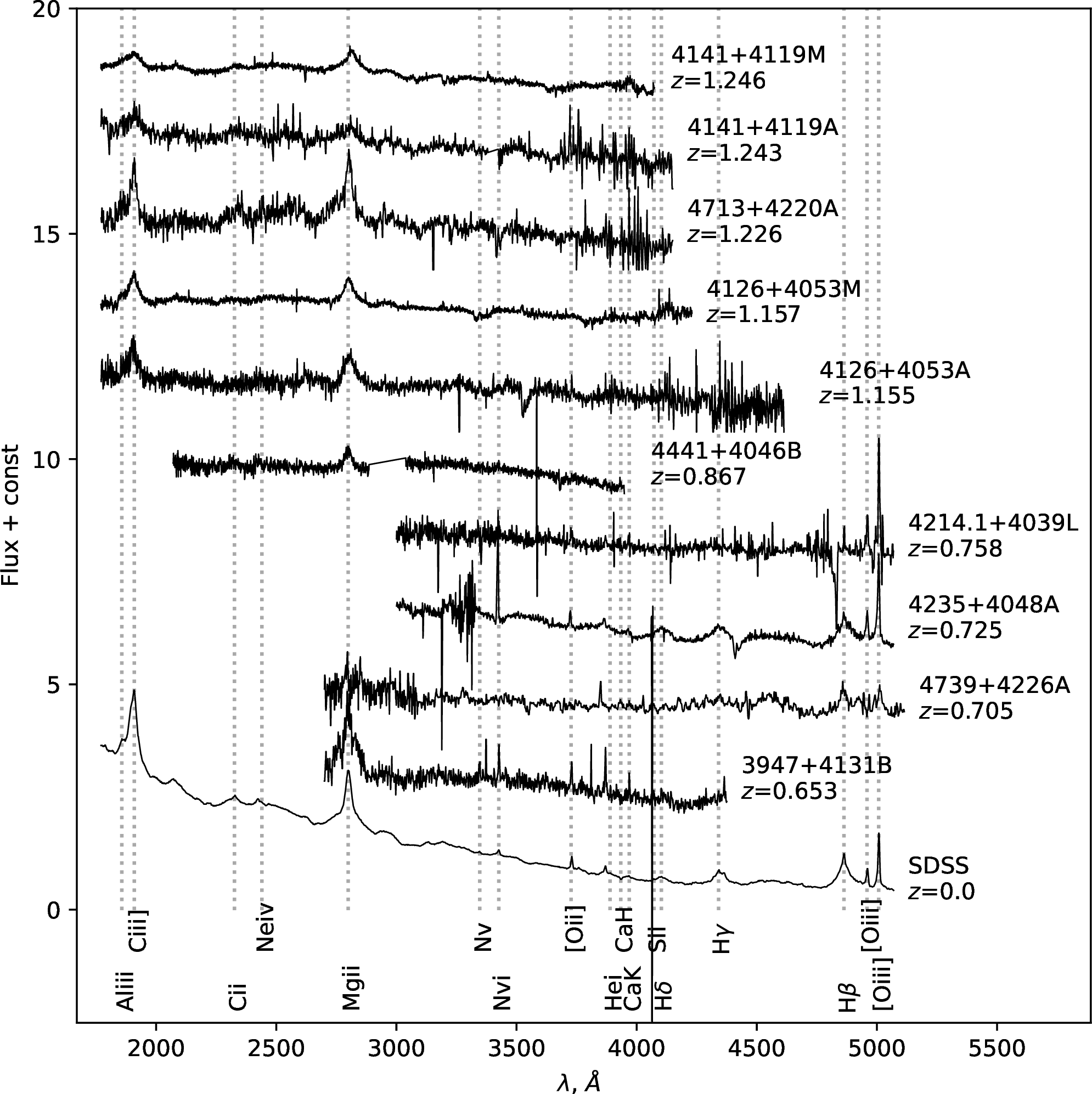
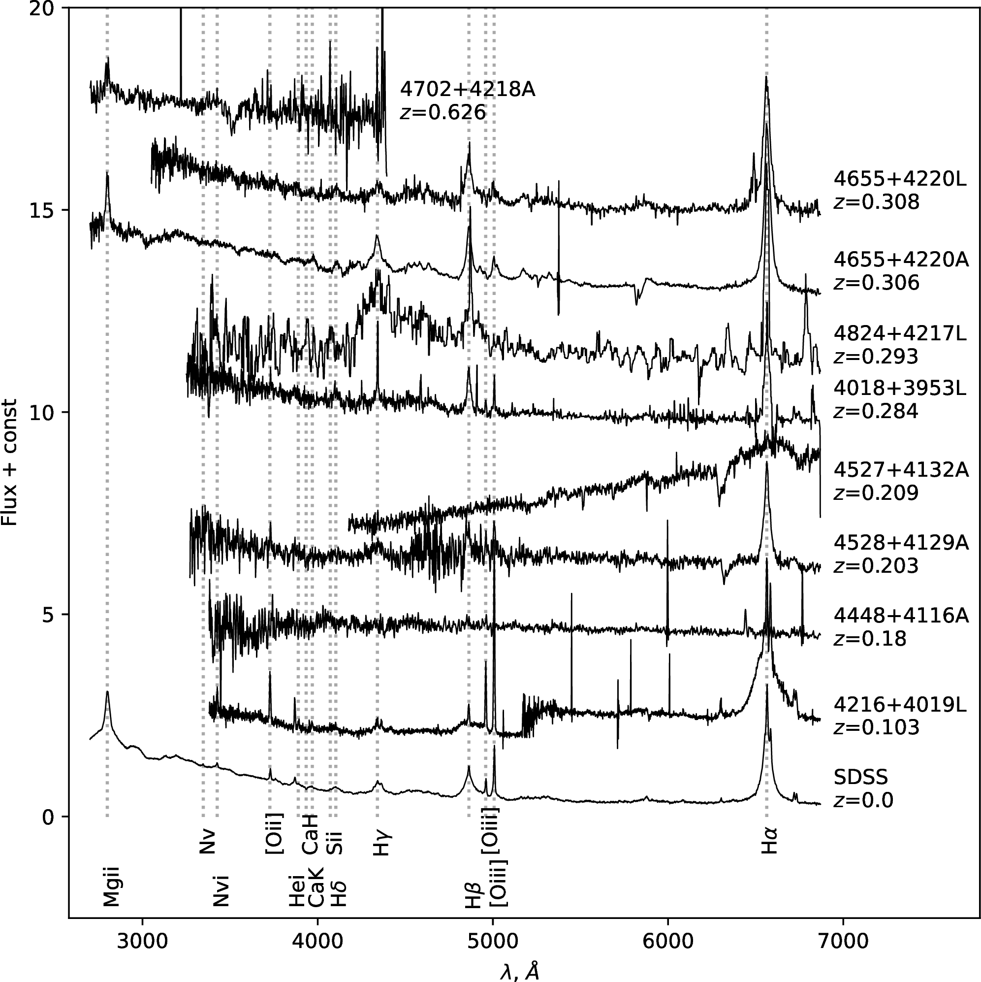
Figure 3: Spectra of the observed objects sorted by redshift, shown at rest frame wavelength. Some more prominent features are marked with vertical dashed lines and are labeled. The SDSS composite quasar spectrum [61] is also plotted at the bottom of each panel..
Broad-band \(grizy\) photometry for the quasars behind M 31 and in the surrounding field was obtained from Pan-STARRS Survey DR1 [52].
4 Quasar sample↩︎
The presence of broad lines in our spectra indicates that 23 (yellow, cyan and black solid dots in Fig. 1) out of the 32 observed objects are quasars; J004029.727+403705.68 and J004215.489+412031.52 (No. 6 and 11 in Table 1, respectively) are new and the rest are confirmations, although for 16 of these our spectra are the first to be published; the 9 non-quasars are stars, galaxies or their nature can not be reliably identified because of the low signal-to-noise of the spectra. Among 13 X-ray selected candidates, 12 turn out to be quasars; the UV excess in LGGS-PHAT selected 4 candidates yielded 2 quasars; the SPITZER-LGGS selected 8 candidates also yielded 3 quasars; 6 of 7 Yuhan Yao objects appear to be quasars. Analyzing 17 more archival spectra, in addition to our data, we uniformly measured redshifts for in total of 34 unique quasars based on 40 spectra in total.
The objects with measured redshift in this work together with the literature QSOs with spectroscopically derived redshift form a sample of 125 QSOs, located within M 31 isophote \(\mu_B\)=26\(^m\)/\(\Box\arcsec\). They are listed in Table ¿tbl:tab:redshifts?, together with the lines used for the redshift measurements and the distances from the M 31 center. For the center of M 31, we adopted the coordinates of its extended core J004244.33+411607.5 [29] located at 1.7\(\arcsec\) from the center defined in RC3 [28]. All distances \(\rho\) within the rectified plane of the galaxy are in fractions, normalized to \(\rho_{25}\), which is the half of the major isophotal diameter D25=190.5\(\arcmin\) measured at surface brightness level \(\mu_B\)=25\(^m\)/\(\Box\arcsec\). They are calculated, assuming position angle PA=35 deg, determined as the ratio of the major-to-minor isophotal diameters R25=3.0903 [28] and taking into account an intrinsic oblateness of 0.14, typical for a Sb galaxy like M 31. Thus, the disk plane is inclined to the line of sight at 17.1 deg.
To outline the area of interest in this work, we tentatively adopted a larger major isophotal diameter of 225\(\arcmin\) as measured approximately at surface brightness level \(\mu_B\)=26\(^m\)/\(\Box\arcsec\) by [27], the same axis ratio and PA as in RC3. Note that the Holmberg diameter of 200\(\arcmin\) [62] falls just between the previous two values, but axis ratio of 2.5 leads to a smaller inclination of 12.1 deg.
![Figure 4: Cross-comparison of redshifts from different sources: z_1 – [51]; z_2 – [43]; z_3 – [37]; z_4 – all other sources (listed in Table ¿tbl:tab:redshifts?), including this work redshift preference when available. Left: z_2, z_3 and z_4 versus z_1. Right: z_3 and z_4 versus z_2. The published measurement errors are shown, except for [37] who do not list them – in this case for plotting purposes we adopted errors equal to 0.005 dex. The bracketed numbers in the legends show how many objects constitute the overlapping subset between each pair of samples. The black dotted line has a slope of one.](/article/2602.20318/redshifts_cross_check_b.png "fig:")
4.1 Redshift measurements↩︎
Quasars are easy to identify from the broad (as wide as thousands of km s\(^{-1}\)) lines, like Civ 1548, Ciii] 1909, Mgii 2799 and others, emitted by the gas in the vicinity of the central supermassive black holes [63], [64].
We measured their redshift following closely the procedures of [20] and [23]. First, we identified the broad lines comparing the spectrum of each object with the composite SDSS quasar spectrum of [61]. Then, we measured the observed wavelengths of the lines fitting Gaussians to them with the IRAF task splot and calculated the redshift of each line. Blended lines were omitted. Lines affected by strong intervening absorption were either omitted, or if possible, Gaussians were fitted only to their cores. The final redshift of an object was determined averaging the redshifts of all emission lines. The redshift uncertainty was the r.m.s. of the individual lines’ redshifts; if only two lines were available, we tentatively adopted as an error the difference between their redshifts.
4.2 Comparison with literature redshifts↩︎
In general, our redshift measurements \(z_4\) shown with dots in Fig. 4 (right), agree well with the literature, with a few exceptions. For example, we measured \(z\)=0.626\(\pm\)0.011 for Gaia DR3 375328395906539392 (Nos. 28 in Table 1 and 109 in Table ¿tbl:tab:redshifts?), while [51] and [43] reported the vastly different \(z\)=2.419\(\pm\)0.016 and \(z\)=1.088\(\pm\)0.188, respectively. We identified the single emission line in its spectrum as Mgii 2799, because no other prominent lines appeared within the wavelength coverage of our APO spectrum, and they should have, if the redshift was different.
For Gaia DR3 375423881617811328 (Nos. 30 in Table 1 and 115 in Table ¿tbl:tab:redshifts?), we measured \(z\)=0.705\(\pm\)0.001, agreeing at \(\sim\)1\(\sigma\) level with \(z\)=0.850\(\pm\)0.147 of [43], but very different from \(z\)=2.880\(\pm\)0.026 of [51]. Our measurement is based on three lines, making the random agreement unlikely.
Gaia DR3 369288714109887744 (Nos. 23 in Table 1 and 92 in Table ¿tbl:tab:redshifts?) is another case of disagreement. This is a rediscovered quasar at z=0.209\(\pm\)0.001 found earlier by [65] at z\(\sim\)0.215. A third measurement of z=1.129\(\pm\)0.008 [51] is considered unreliable.
The largest redshift discrepancy is associated with Gaia DR3 381231021002898048 (Nos. 1 in Table 1 and 15 in Table ¿tbl:tab:redshifts?). Our higher quality SAO spectrum yields 1.425\(\pm\)0.005, very different from z=4.619\(\pm\)0.042 of [51]. Notably, this work gives some extremely high redshifts – with respect to [43] – for other 21 qausars.
For two objects, we measured redshifts higher than the values of [51]. For DR3 375418590218050304 (Nos. 32 in Table 1 and 118 in Table ¿tbl:tab:redshifts?), they reported \(z\)=0.341\(\pm\)0.003, while we measured \(z\)=0.769\(\pm\)0.002, very similar to \(z\)=0.798\(\pm\)0.328 of [43]. The decisive argument for our higher redshift is the identification of Mgii 2799 in the blue arm of the APO spectrograph. The two arms are calibrated independently, in effect they are two instruments.
For Gaia DR3 381223637953333376 (Nos. 3 in Table 1 and 18 in Table ¿tbl:tab:redshifts?), we measured \(z\)=1.570\(\pm\)0.001. [51] place it at \(z\)=0.101\(\pm\)0.008 – inconsistent with our excellent quality SAO spectrum that exhibits multiple emission lines.
Not surprisingly, somewhat better agreement exists between \(z_3\) [37] and \(z_2\) [43], and between our redshifts \(z_3\) and \(z_2\) [43] as seen in Fig. 4, right. The only inconsistent case here is Gaia DR3 381137287633113216 (No. 7 in Table ¿tbl:tab:redshifts?): [43] reported \(z\)=1.060\(\pm\)0.209, very different from our value of \(z\)=2.868\(\pm\)0.003. Our value agrees with three other measurements from the literature.
The blazar Gaia DR3 375378320605062144 [33] was excluded from our redshift and reddening analyses, because of the contradicting \(z\) measurements in the literature and because it may not exhibit typical quasar colors.
Some objects were misidentified as quasars in the literature. [26] reported that LAMOST_10.952+40.80076 (Gaia DR3 369228137893480064) is a QSO at \(z\)=0.262. However, a careful inspection of the LAMOST DR5 spectrum (spec-55859-M5901_sp04-015) revealed prominent CaT and other stellar features typical for K7-M0 stars. Another example is Gaia DR3 381200372113648128, listed as J003905.66+410456.6 in LAMOST DR2&3 [30] and LAMOST_9.774+41.08240 in LAMOST DR4 [26]. We did not find convincing confirmation of the \(z\) \(\sim\)0.8 derived in both these papers from the LAMOST spectra. Instead, we identified a broad feature corresponding to H\(\alpha\) at the M 31 rest frame and we suspected that it has been misinterpreted as Civ 1548 by [51] who reported \(z\)=3.190\(\pm\)0.027.
Our selection identified 9 more QSO candidates within the \(\mu_B\)=26\(^m\)/\(\Box\arcsec\) isophote and we observed them (Nos. 5, 7, 13–17, 19, 26 in Table 1), but the spectra did not provide evidences for a quasar nature. This was the case with object No. 16, located in a prominent dust lane. [66] reported \(\sim\)10% probability that it is a galaxy. However, our spectrum lacks broad emission lines and shows absorptions making it a likely red star or a globular cluster in M 31. These nine and the two LAMOST objects mentioned above were omitted from Table ¿tbl:tab:redshifts?.
The heterogeneous nature of the selection and the lack of comparison quasars outside of the M 31 disk, confirmed by the same means and following the same strategy makes it difficult to estimate the completeness of this sample. The only exception, and the largest contribution to our sample – bringing in about 2/3 of the quasars – is the all-sky Quaia survey. We compared the surface density of secure quasars, according to the classification of [51], see their Class, reproduced here in Table ¿tbl:tab:redshifts?. There is an 10-30% excess of such objects inside of the \(\mu_B\)=26\(^m\)/\(\Box\arcsec\) isophote, where the exact percentage depends on the adopted outside locus and magnitude limits. Therefore, it is not the incompleteness but rather the contamination that may be an issue for quasar searches, underlying the need for reliable spectroscopic confirmation like the follow up we report here.
4.3 Reliability of redshift measurements↩︎
To assess the reliability of heterogeneous literature redshifts, we compared the multiple measurements that are available for some sources (Fig. 4). [51] reported some relatively high redshift measurements that found no confirmation among other sources (pale blue dots on the left panel). Many outliers in Fig. 4 (left) have a probability \(P_{QSO}\) of being a quasar \(\sim\) 100\(\%\) questioning the reliability of P\(_{QSO}\) and the values or of their redshitfs. Further investigation revealed that these high redshifts are associated with objects not classified as active galaxies or all together lacking classification in [51], again, refer to the Class in Table ¿tbl:tab:redshifts?. Therefore, the redshifts in Gaia DR3 must be treated with caution, unless the object is specifically classified as a high-probability active galaxy.
Other literature sources agreed better between themselves. For example [21] finds good agreement between their own redshifts and the Quaia measurements. However, taking the literature redshifts at face value seems risky. To ensure we use the most reliable redshifts, we adopted the following strategy: if an individual redshift measurement for an object is available, e.g. from our own spectra or from the literature, we prefer this value, because these as a rule are human-verified, as opposed to redshifts from large surveys that rely – as a rule – on automated procedures. This is largely driven by our concern about the objects with \(z\) \(>\)3 of [51]. In total 18 quasars fall into this group. Note that some of the spectra come from the literature, but we reidentified the emission lines and remeasured the redshifts.
If no individual measurements were available, we turned to survey data, in order of preferences: [37], [43]. These two surveys contributed 9 and 81 redshifts, respectively. This brings the total number of quasars with spectroscopic redshifts within the \(\mu_B\)=26\(^m\)/\(\Box\arcsec\) isophote to 124, omitting the blazar, as discussed earlier.
5 M 31 disk extinction↩︎
We attempted to measure the extinction within the M 31 disk from the color excess of quasars within the \(\mu_B\)=26\(^m\)/\(\Box\arcsec\) isophote with respect to the colors of quasars at similar redshift, located away from M 31, assuming that they show on average the same colors, as long as they are at the same redshift, and that the large number of quasars away from the disk will average out any intrinsic variations.
First, we correct both quasar samples for the foreground Milky Way extinction. Outside of M 31, we apply individual estimates from the map of [67]. Within the M 31 body, the predicted E(\(B\) \(-\) \(V\)) increases inwards – due to the dust content of the galaxy itself. To alleviate this issue, we adopted for all objects inside the \(\mu_B\)=26\(^m\)/\(\Box\arcsec\) isophote a constant foreground Milky Way extinction. We considered 326 Quaia quasars within an elliptical annulus between one and two major-axis D26 isophotal diameters, to ensure that they are safely clear of M 31, but still in the general direction of the galaxy, minimizing any residual Milky Way extinction. Averaging the individual extinctions, we derived E(\(B\) \(-\) \(V\))=0.060\(\pm\)0.010 mag, similar to E(\(B\) \(-\) \(V\))=0.055 mag that [67] report for the M 31 center and well within the range 0.035\(-\)0.105 mag that the same map enables.
![Figure 5: Intrinsic colors of our Quaia reference quasar sample, obtained after correcting the Pan-STARRS Survey DR1 grizy photometry [52] for the Milky Way extinction according to the [67]. The color of the points marks the distance of the quasars from the M 31 center \rho in units of \rho_{25} isophotal radii. The distance bins’ widths were set to ensure these bins contain similar number of quasars. The solid lines connect the medians colors within 0.5 dex wide redshift bins. The vertical error bars are the standard deviations of the colors of all quasars within each redshift bin, regardless of the distance from the M 31 center, and they were calculated as 1.48\timesMAD (median absolute deviation), to suppress the influence of outliers.](/article/2602.20318/colors_dered.png "fig:")
Next, we derived the intrinsic colors (\(g\) \(-\) \(r\))\(_0\), (\(g\) \(-\) \(i\))\(_0\), (\(g\) \(-\) \(z\))\(_0\) and (\(g\) \(-\) \(y\))\(_0\), at the redshift of each quasar behind M 31, as median over the dereddened colors of all quasars in the reference sample with redshift within 0.3 dex (Fig. 5). This reference sample was selected from the Quaia catalog to include all quasars within 5 deg from the M 31 center (about 2600 objects in total, see Fig. 5 for the exact numbers in the individual colors), but outside the \(\mu_B\)=26\(^m\)/\(\Box\arcsec\) isophote, to ensure averaging over 100’s of quasars. We converted the color excesses to A\(_V\) adopting a total-to-selective extinction ratio R\(_V\)=3.1 and according to the extinction law of [68]. We formed the A\(_V\) error for each quasar behind M 31 as a quadrature sum of the quasars’ photometric errors and the variation of the intrinsic colors for the quasars at that redshift. We averaged the derived A\(_V\)’s from the four colors with error weighting. Some extinctions are negative because of the large intrinsic spread of quasar colors that can be seen in Fig. 5 and to lesser extend, the photometric errors. Furthermore, undetected contamination from blue foreground objects in M 31 itself may also lead to negative extinction, although we tried to exclude this by selecting isolated candidates for the follow up. No trend in the evolution of the broad band intrinsic colors of quasars as a function of redshift is seen when the sample is divided into several radial bins spanning 1.5 to 11 \(\rho_{25}\).10
We used two M 31 extinction maps to compare our estimates with. The map of [69] has the SPIRE 350 resolution of 25\(\arcsec\). It gives the dust surface density and its uncertainty in units of (\(M_{\odot}/kpc^2\)). We converted these quantities into absorption \(A_V\) values according to the [70] dust model. The map of [71] has 7\(\arcsec\) resolution. It derives A\(_V\) using stellar photometry of red giant branch (RGB) stars from [34] survey, enabling a direct comparison with our results. Only 114 of our quasars fall within the footprint of the former map and 14 – of the latter. No correlation is found in both cases (Fig. 6). This negative result is probably due mostly to the bias towards lower extinction that is rooted in the quasar selection and especially in the target selection for the spectroscopic confirmation: quasars located along more heavily obscured lines of sight are fainter and less likely to have spectra. This can be seen in Fig. 7 that overplots the quasars in the sample on the [69] reddening map. Furthermore, with quasars we measure the extinction along a narrow line of sight, while the reddening maps average the extinction over wider bins. Last but not least, the number of quasars may be insufficient for this test, considering the significant variation of the quasar’s intrinsic colors (Fig. 5).
![Figure 6: Comparison of A_V derived from our quasar sample and from the reddening maps of [69] and [71].](/article/2602.20318/Av_quasars_vs_Av_maps.png "fig:")
![Figure 7: Location of the quasars from our sample on the reddening maps (green open circles) of [69] and [71].](/article/2602.20318/Draine_map2.png "fig:")
6 Summary and conclusions↩︎
We selected quasar candidates from apparent colors and X-ray emission among objects within the M 31 \(\mu_B\)=26\(^m\)/\(\Box\arcsec\) isophote and carried out optical spectroscopy of the brightest of them to confirm their nature increasing the number of published spectra from 24 to 40. We also collected quasars from various public surveys, bringing the total number of bona-fide quasars behind the M 31 disk to 124 (125, counting one blazar).
Our work provides a large sample of quasars for astrometric studies of M 31 [72], similar to the previous work in the Magellanic clouds [73]. Quasars facilitate also studies of its interstellar medium (ISM) – both of the extinction from their colors, as we attempted to do here, and of the ISM’s chemical abundances with spectroscopy, typically in the UV [8], [74]. The later work will come within reach for many faint quasars with the next generation of 30-40-m class spectroscopic telescopes or with the dedicated spectroscopic facilities, such as the WST [Wide-field Spectroscopic Telescope; [75]].
We measured the extinction inside M 31 towards 114 quasars with reliable redshifts and found no correlation with the existing reddening maps, probably because of the limited number of objects, the biases in our sample, and different physical scales of the regions that are probed with the quasars and the dust maps. This problem must be revisited when LSST helps to discover more quasars, based on their variability, as [20], [21] demonstrated that the variability helps to increase the efficiency of quasar selection.
Last but not least, in the course of our analysis we confirmed the previous concerns that the redshifts, derived from low-resolution spectra may contain significant errors. Such measurements must be treated with caution.
The authors thank an anonymous referee whose valuable comments and recommendations helped to improve the quality of the paper. PN and AV acknowledge financial support from the European Union-NextGenerationEU, through the National Recovery and Resilience Plan of the Republic of Bulgaria, project No BG-RRP-2.004-0008-C01. PN thanks Phillip Massey for sharing the spectra of 10 QSOs behind the disk of M 31 obtained with Hectospec at the MMT. PN is also grateful to Julianne Dalcanton for providing the extinction maps of the M 31 disk, based on the PHAT survey data. The search for QSOs behind the disc of the M 31 galaxy was partially supported by a short-term scholar Fulbright grant of PN at the Department of Astronomy, University of Washington, for the academic year 2018–2019 from the US Department of State program number G-1-00005. This work has made use of data from the European Space Agency (ESA) mission Gaia (https://www.cosmos.esa.int/gaia), processed by the Gaia Data Processing and Analysis Consortium (DPAC, https://www.cosmos.esa.int/web/gaia/dpac/consortium). Funding for the DPAC has been provided by national institutions, in particular the institutions participating in the Gaia Multilateral Agreement. Observations with the SAO RAS telescopes are supported by the Ministry of Science and Higher Education of the Russian Federation. The renovation of telescope equipment is currently provided within the national project “Science and Universities”. The BTA data reduction was performed as part of the SAO RAS government contract approved by the Ministry of Science and Higher Education of the Russian Federation. This work uses data from the Guoshoujing Telescope (the Large Sky Area Multi-Object Fiber Spectroscopic Telescope LAMOST). It is a National Major Scientific Project built by the Chinese Academy of Sciences. Funding for the project has been provided by the National Development and Reform Commission. LAMOST is operated and managed by the National Astronomical Observatories, Chinese Academy of Sciences.
\begin{table}[!ht]
}\end{table}
\begin{table}[!ht]
}\end{table}
\begin{table}[!ht]
}\end{table}
\begin{table}[!ht]
}\end{table}
\begin{table}[!ht]
}\end{table}
\begin{table}[!ht]
}\end{table}
\begin{table}[!ht]
}\end{table}
\begin{table}[!ht]
}\end{table}
\begin{table}[!ht]
}\end{table}
7 Data availability↩︎
Table ¿tbl:tab:data95spectra? lists the spectra that are reported for the first time in this paper.
| \(\lambda\) [Angström] | Flux [arbitrary units] |
|---|---|
| J004029.727+403705.68 | |
| 3533 | 1.104 |
| 3535 | 1.222 |
| 3537 | 0.995 |
| 3538 | 1.229 |
| 3540 | 1.041 |
| 3542 | 0.960 |
| 3544 | 1.293 |
| ... | |
| J004215.487+412031.52 | |
| 3801 | 0.429 |
| 3803 | 1.196 |
| 3805 | 1.275 |
| 3807 | 1.742 |
| 3809 | 0.767 |
| 3811 | 1.595 |
| 3813 | 2.027 |
| ... | |
8 Intrinsic colors of quasars↩︎
Table ¿tbl:tab:quasar95colors? lists the derived intrinsic colors of quasars, as shown with black lines in Fig. 5.
| \(z\) | (\(g\)\(-\)\(r\)) [mag] | (\(g\)\(-\)\(i\)) [mag] | (\(g\)\(-\)\(z\)) [mag] | (\(g\)\(-\)\(y\)) [mag] | N |
|---|---|---|---|---|---|
| 0.1 | 0.222\(\pm\)0.151 | 0.569\(\pm\)0.258 | 0.586\(\pm\)0.239 | 0.697\(\pm\)0.286 | 8 |
| 0.3 | 0.266\(\pm\)0.201 | 0.408\(\pm\)0.305 | 0.800\(\pm\)0.264 | 0.612\(\pm\)0.402 | 79 |
| 0.5 | 0.062\(\pm\)0.168 | 0.312\(\pm\)0.258 | 0.297\(\pm\)0.321 | 0.694\(\pm\)0.272 | 138 |
| 0.7 | 0.061\(\pm\)0.120 | 0.138\(\pm\)0.213 | 0.254\(\pm\)0.224 | 0.251\(\pm\)0.298 | 187 |
| 0.9 | 0.118\(\pm\)0.163 | 0.118\(\pm\)0.235 | 0.190\(\pm\)0.251 | 0.306\(\pm\)0.294 | 249 |
| 1.1 | 0.250\(\pm\)0.118 | 0.229\(\pm\)0.173 | 0.159\(\pm\)0.193 | 0.319\(\pm\)0.223 | 273 |
| 1.3 | 0.262\(\pm\)0.124 | 0.287\(\pm\)0.182 | 0.257\(\pm\)0.193 | 0.314\(\pm\)0.197 | 270 |
| 1.5 | 0.193\(\pm\)0.130 | 0.349\(\pm\)0.160 | 0.327\(\pm\)0.167 | 0.339\(\pm\)0.216 | 295 |
| 1.7 | 0.081\(\pm\)0.116 | 0.301\(\pm\)0.174 | 0.286\(\pm\)0.160 | 0.329\(\pm\)0.210 | 262 |
| 1.9 | 0.078\(\pm\)0.119 | 0.260\(\pm\)0.148 | 0.337\(\pm\)0.174 | 0.392\(\pm\)0.196 | 222 |
| 2.1 | 0.092\(\pm\)0.111 | 0.178\(\pm\)0.162 | 0.357\(\pm\)0.179 | 0.367\(\pm\)0.197 | 173 |
| 2.3 | 0.076\(\pm\)0.116 | 0.151\(\pm\)0.145 | 0.325\(\pm\)0.177 | 0.442\(\pm\)0.171 | 174 |
| 2.5 | 0.080\(\pm\)0.121 | 0.123\(\pm\)0.162 | 0.235\(\pm\)0.157 | 0.440\(\pm\)0.164 | 124 |
| 2.7 | 0.136\(\pm\)0.134 | 0.213\(\pm\)0.178 | 0.280\(\pm\)0.161 | 0.434\(\pm\)0.223 | 94 |
| 2.9 | 0.119\(\pm\)0.119 | 0.225\(\pm\)0.163 | 0.204\(\pm\)0.165 | 0.377\(\pm\)0.131 | 62 |
| 3.1 | 0.248\(\pm\)0.085 | 0.361\(\pm\)0.223 | 0.306\(\pm\)0.201 | 0.467\(\pm\)0.160 | 34 |
9 Correction of the Spitzer coordinates↩︎
The coordinate accuracy of candidate quasars is crucial for their cross-identification for the optical spectroscopic follow up. Most of our candidates are selected on the base of their Spitzer photometry [35], but a comparison with various near-infrared and optical catalogs revealed systematic offsets in this coordinate system. Therefore, we decided to transfer the Spitzer coordinates of [35] to the WISE J2000 coordinate system. We cross-matched the Spitzer and WISE coordinates with 3\(\arcsec\) matching radius, for objects with [W2]\(\leq\)13.5 mag and –0.35 mag\(\leq\)[W2]–[W1]\(\leq\)0.35 mag as shown in Fig. 2 (top right panel), to ensure we only consider high signal-o-noise detections and to reduce the number of spurious matches. Then, we formed the Spitzer–WISE coordinate differences \(\delta\)RA and \(\delta\)DEC, for these sources, plotted them versus each other (Fig.8, top left) and saw a two-clump structure. We imposed an initial separation between the two clumps along the blue line. The objects above and below it (plotted everywhere with black and red dots, respectively) are located into two distinct spatial regions on the sky, separated with a line connecting the following positions in RA, DEC (J2000), in degrees: (9.714, 41.195), (10.140, 41.048), (10.963, 41.874), (11.685, 41.874), (11.920, 42.010) and (12.186, 42.005) – marked with green solid line in Fig. 9. For all objects within each of these two areas we derived separately polynomial fits, with 3-\(\sigma\) clipping, of \(\delta\)RA and \(\delta\)DEC versus DEC and RA, respectively (Fig.8, middle and lower panels), based on about 1600 objects in total: \[\delta DEC_{black}=-1.671+0.36211\times RA-0.014715\times RA^2\] \[\begin{align} \delta DEC_{red}=-405.401+107.03023\times RA-9.006573\times RA^2\\ +0.2022619\times RA^3+0.00327904\times RA^4 \end{align}\] \[\begin{align} \delta RA_{black}=-26974.840+1920.434447\times DEC \\ -45.5512001\times DEC^2+0.35995935\times DEC^3 \end{align}\] \[\begin{align} \delta RA_{red}=8571.288-620.935448\times DEC \\ +15.0056471\times DEC^2 -0.12096752\times DEC^3 \end{align}\] The typical RMS of these relations is \(\sim\)0.3. Applying them brings the two clumps together (Fig.8, upper right panel).
A minor caveat in this correction is the omission of the proper motions of the brightest sources that are probably Milky Way stars, but the Gaia DR3 suggests there are of order of 10-20 mas yr\(^{-1}\). Fortuitously, the Spitzer–WISE time baseline is \(\sim\) 5 yr , so any cumulative effect from the proper motions can safely be neglected.
![Figure 8: Upper left: \deltaRA/\deltaDEC plot for the astrometric Spitzer–WISE comparison of 1623 objects from our bright astrometric sample. The double central clump is due to small systematic deviations in the [35] coordinate system. The blue line makes initial division of the astrometric sample into two spatially distinct sub-samples of \sim700 and \sim900 objects (see Fig. 9). Upper right: the same plot after 3\sigma clipping and correcting for the systematic effect to the WISE coordinate system. Middle: \deltaDEC(Spitzer–WISE) versus WISE RA. Bottom: \deltaRA(Spitzer–WISE) versus WISE DEC. The solid and dashed green curves are the best fits to the trends for the two sub-samples on the middle and bottom panels (see text).](/article/2602.20318/fa_delta-delta.png "fig:")
![Figure 9: Map of our astrometric sample of 1623 objects with the adopted final dividing solid line (solid green) for the two spatially distinct samples of 710 (red dots) and 913 (black dots) objects. The dashed line shows the approximate outline of [35] catalog, the solid and dotted lines show the \mu_B=26^m/\Box\arcsec and \mu_B=25^m/\Box\arcsec isophotes, respectively. M 31 center is marked with an x.](/article/2602.20318/astro_radec.png "fig:")
References↩︎
Here, we use quasar, QSO and AGN interchangeably, because determining the exact energetics of each object is beyond the scope of this work. Furthermore, the observed broad emission lines indicate that our sample is dominated by Type 1 QSOs.↩︎
https://speakerdeck.com/yaoyuhan/quasars-behind-m31-from-ptf-survey↩︎
IRAF is distributed by the National Optical Astronomy Observatory, which is operated by the Association of Universities for Research in Astronomy under a cooperative agreement with the National Science Foundation.↩︎
A stand-alone Python script that derives the intrinsic colors of quasars as a function of redshift from a sample of references quasars outside M 31, and then calculates the color excesses and absorptions for individual quasars behind the M 31, is available at https://github.com/vdivanov/Quasars_behind_M31_2026/, together with the necessary input files.↩︎