1 Introduction↩︎

Cauchy matrices are a family of structured matrices appearing in interpolation and approximation problems with rational functions. Moreover, they belong to the class of displacement structured matrices and, as such, they share notable computational properties with other structured matrix families, e.g., Toeplitz, Vandermonde, and Hankel matrices [1]. In fact, several algebraic computations involving Cauchy matrices can be performed efficiently using fast algorithms [2]. This is because, although a Cauchy matrix is fully populated by nonzero entries, it can be exactly described by a set of parameters growing linearly with the dimension. Cauchy matrices have been characterized in [3] as transition matrices between the eigenbases of two diagonalizable matrices that differ by a rank-one term. Moreover, row- and column-scaled versions of Cauchy matrices also appear in the numerical solution of secular equations and as eigenvector matrices of particular symmetric quasiseparable matrices [4].

The present work is motivated by the results of Liesen and Luce [5], who addressed the problem of determining whether a given matrix is Cauchy or can be approximated by a matrix with that structure. To this goal, the authors of [5] presented two algorithms. The first determines the parameters that define a Cauchy matrix using only the values in its first row and column. The second computes the parameters of a Cauchy matrix that best approximates a perturbed data matrix, in some sense. Both algorithms have optimal complexity, and the second is accompanied by a posteriori error bounds, i.e., upper bounds on the approximation errors based on the evaluation of suitably defined residuals. These algorithms are based on a characteristic property of Cauchy matrices: the matrix obtained by entrywise reciprocation is rank-two and has a specific structure. Therefore, the problems discussed by Liesen and Luce are somewhat related to the issue of representing rank-two matrices appropriately. In the case of generic matrices with non-negative elements, this latter problem is addressed in great depth in [6].

The problem of reconstructing a matrix having some kind of structure from noisy data is a well-known topic in numerical linear algebra that has been developed recently along different directions, because of the applications in mathematical modeling, signal processing, data compression, time series analysis, etc. For example, in [7] the authors address the problem of best approximation of a given matrix by a matrix of lower rank in the elementwise maximum norm. Comprehensive summaries on the construction of a structured low-rank matrix that is nearest to a given matrix are given in [8], [9]. Also the reconstruction of perturbed matrices with displacement structures, notably Toeplitz, Hankel, and Vandermonde matrices, has received some attention, see e.g., [10]–[12]. The computational approaches are usually based on the minimization of a possibly non-convex objective functional which measures the error between the data matrix and the approximating one, which may be subject to both rank and structural constraints. Analogous techniques are also employed for solving completion problems with displacement structured matrices, see [13].

In this work, we take a deeper look at the problem of recovering a Cauchy matrix from perturbed data. After collecting some preliminary notions and results on Cauchy matrices in the next section, Section 3 proposes a unified framework for the description and analysis of the algorithms in [5], based on a suitable family of projectors onto a subspace of rank-2 matrices. This framework allows us to introduce a parametrized algorithm, here called Algorithm 3, for solving our parameter recovery problem that includes both algorithms discussed by Liesen and Luce as particular cases. Moreover, we provide error bounds on the recovered parameters that are a priori, that is, intrinsic to the algorithm and do not depend on residual norms. For notational simplicity, we limit ourselves to considering real square matrices. Extending our results to rectangular and complex matrices only requires straightforward notational amendments and minor adaptations. On the other hand, we consider measuring approximation errors in both the Frobenius norm and the elementwise maximum norm.

Section 4 provides a further analysis of Algorithm 1 in [5] that relies on CUR factorization theory and provides new error estimates that involve singular values of an augmented matrix. In Section 5 we formulate a measure of ‘Cauchyness’ based on the displacement characterization of the Cauchy structure, and propose a recovery strategy based on the minimization of that measure, which leads to Algorithm 4. Finally, we present in Section 6 the results of a series of numerical experiments to illustrate the performance of the various algorithms on perturbed Cauchy matrices. As a side note, we discuss in the Appendix a parametrization of (entrywise reciprocated) Cauchy matrices that is perfectly well conditioned. Compared to the one originally presented in [5], the new parametrization has a tighter error bound when recovering a perturbed Cauchy matrix via Algorithm 2.

1.1 Notation↩︎

The following notation will be used throughout this paper. The maximum (Chebyshev) norm and the Frobenius norm of a matrix \(A\in{\mathbb{R}}^{n\times n}\) are defined as \[\|A\|_{\max}= \max_{i,j=1,\ldots,n}|A_{ij}| , \qquad \|A\|_\mathrm{F}= \bigg(\sum_{i,j=1}^n A_{ij}^2\bigg)^{1/2} ,\] respectively. We sometimes use the symbol \(\|\cdot\|_\star\) to denote any of the above matrix norms. These norms share the property presented in the following lemma.

An \(n\times n\) identity matrix is denoted \(I_n\) or simply \(I\) if the size is evident. The symbol \(\mathbf{1}\) denotes the all-ones vector of appropriate size, \(\mathbf{1}=(1,\ldots,1)^T\in{\mathbb{R}}^n\). We also write \(\mathbf{1}_n\) to explicitly indicate the size. Denote as \(\mathrm{vec}\) the vectorization operator such that \(\mathrm{vec}(A)\) is the vector in \({\mathbb{R}}^{n^2}\) obtained by stacking the columns of \(A\). Note that \(\|A\|_{\max}= \|\mathrm{vec}(A)\|_\infty\) and \(\|A\|_\mathrm{F}= \|\mathrm{vec}(A)\|_2\). The symbol \(\otimes\) denotes the Kronecker product. The following well-known identity establishes a relationship between matrix multiplication, Kronecker product, and vectorization: \[\label{eq:ABC} \mathrm{vec}(ABC) = (C^T\otimes A)\mathrm{vec}(B) .\tag{1}\] Let \(M\) and \(N\) two matrices with the same number of columns. The Matlab-style notation \([M;N]\) denotes the matrix obtained by stacking \(M\) on top of \(N\). Conversely, if \(M\) and \(N\) have the same number of rows then \([M\;N]\) indicates the matrix obtained by concatenating the rows of \(M\) and \(N\). For a matrix \(X\in{\mathbb{R}}^{n\times n}\) with no zero entries we denote as \({X}^{[-1]}\in{\mathbb{R}}^{n\times n}\) the entrywise reciprocal matrix, \[{X}^{[-1]}_{ij} = 1/X_{ij} .\] For any vector \(x\in{\mathbb{R}}^n\) we denote \(\mathrm{Diag}(x)\) the \(n\times n\) diagonal matrix with the entries of \(x\) in the main diagonal.

2 Preliminaries on Cauchy matrices and the recovery of Cauchy points↩︎

A matrix \(C \in{\mathbb{R}}^{n\times n}\) is a Cauchy matrix if \[C_{ij} = \frac{1}{x_i-y_j}\] for real numbers \(x_1,\ldots,x_n\) and \(y_1,\ldots,y_n\) such that \(x_i \neq y_j\) for \(i,j=1,\ldots,n\). We say that the vectors \(x = [x_i]_{i=1,\ldots,n}\) and \(y = [y_i]_{i=1,\ldots,n}\) are Cauchy points of the matrix \(C\), and we adopt the notation \(C = \mathop{\mathrm{\tt Cauchy}}(x,y)\). Note that the Cauchy points are defined up to an additive constant. In fact, it is not hard to check that \(\mathop{\mathrm{\tt Cauchy}}(x,y) = \mathop{\mathrm{\tt Cauchy}}(x+\alpha\mathbf{1},y+\alpha\mathbf{1})\) for every \(\alpha\in{\mathbb{R}}\). Following [5] we say that the Cauchy points \(x\) and \(y\) of a Cauchy matrix \(C\) are normalized if \(\sum_{i=1}^n (x_i^2 + y_i^2)\) is minimal among all possible Cauchy points. It can be easily verified that, given \(C = \mathop{\mathrm{\tt Cauchy}}(x,y)\), the vectors \(\hat{x} = x -\alpha\mathbf{1}\) and \(\hat{y} = y -\alpha\mathbf{1}\) with \(\alpha = \sum_i(x_i+y_i)/(2n)\) are the normalized Cauchy points of \(C\).

Let \(\mathcal{D}\subset {\mathbb{R}}^{n\times n}\) be the set \[\label{eq:defD} \mathcal{D} = \{ x\mathbf{1}^T - \mathbf{1}y^T\in{\mathbb{R}}^{n\times n}\, |\, x,~y\in{\mathbb{R}}^n\} ,\tag{2}\] which is a vector subspace of \({\mathbb{R}}^{n\times n}\) of dimension \(2n-1\). Based on this definition, we can say that a matrix \(A \in{\mathbb{R}}^{n\times n}\) is a Cauchy matrix if and only if it has no zero entries and \({A}^{[-1]}\in\mathcal{D}\). Let us also introduce the matrix-valued operator \(\Delta:{\mathbb{R}}^n\times {\mathbb{R}}^n\mapsto{\mathbb{R}}^{n\times n}\) defined as \[\Delta(x,y) = x\mathbf{1}^T - \mathbf{1}y^T .\] It holds \(\mathrm{Range}(\Delta) = \mathcal{D}\). Moreover, if \(x,y\) are Cauchy points then \(\mathop{\mathrm{\tt Cauchy}}(x,y) = {\Delta(x,y)}^{[-1]}\). However, not all matrices in \(\mathcal{D}\) are entrywise reciprocals of Cauchy matrices. We call generators of a matrix \(D\in\mathcal{D}\) any vector pair \((x,y)\) such that \(D = \Delta(x,y)\). Furthermore, we say that \((x,y)\) are normalized if \(\sum_{i=1}^n (x_i^2 + y_i^2)\) is minimal.

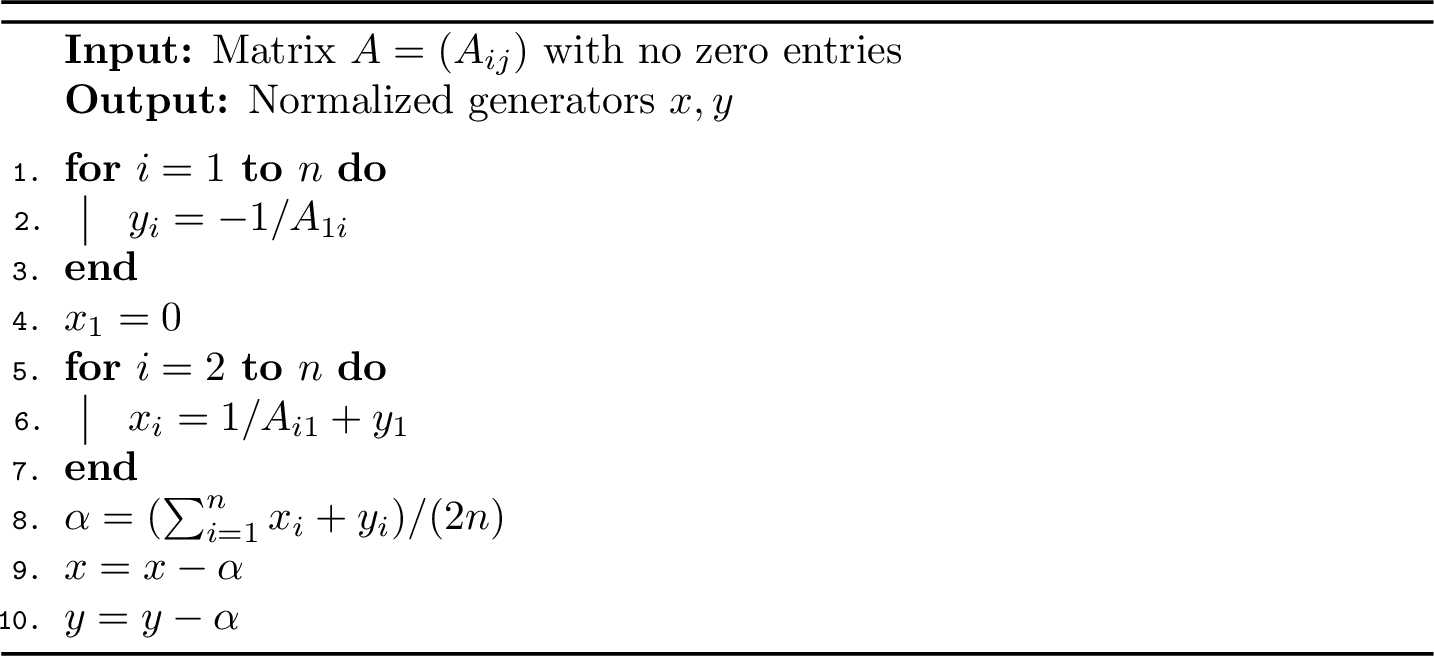
The following Algorithm 1, borrowed from [5], recovers the normalized Cauchy points of a given Cauchy matrix. The computed vectors \(x\) and \(y\) are identified by equating the entries in the first row and column of \(\Delta(x,y)\) and the entrywise inverse of the input matrix. If the input matrix \(A\) is Cauchy then \(x\) and \(y\) are normalized Cauchy points such that \(A = \mathop{\mathrm{\tt Cauchy}}(x,y)\). However, Algorithm 1 can also be applied to a generic matrix with nonzero entries, in which case the vectors \(x\) and \(y\) are normalized generators of a matrix in \(\mathcal{D}\).

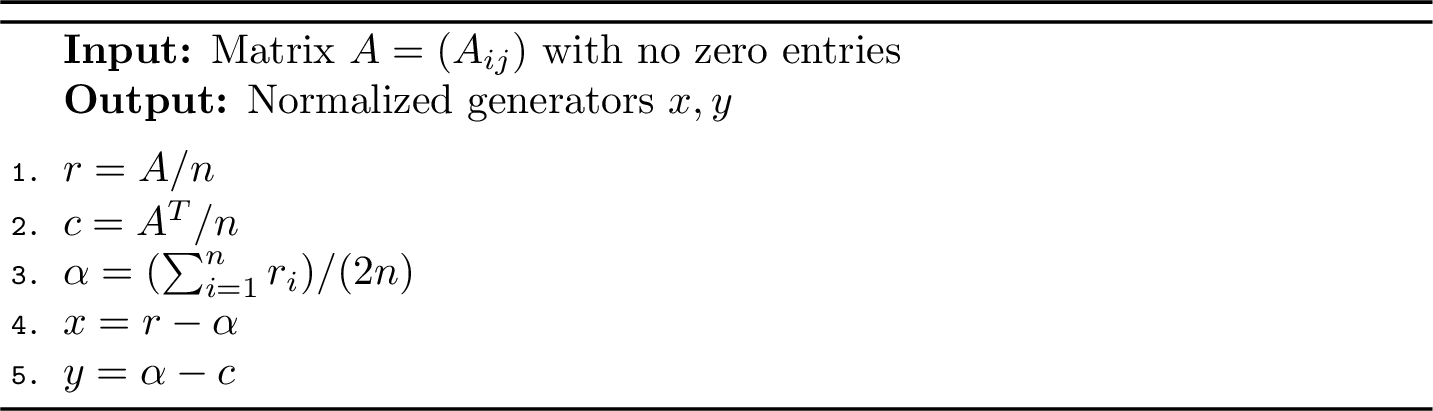
Now, suppose that \(A\) is a perturbed Cauchy matrix, that is, \(A = B + E\) where \(B\) is Cauchy and \(E\) is a perturbation matrix with ‘small’ entries. Aiming at recovering the matrix \(B\), the authors of [5] propose the Algorithm 2 below which computes vectors \(x\) and \(y\) such that \(\Delta(x,y)\) is the solution of \[\label{eq:minF} \min_{X\in\mathcal{D}}\|{A}^{[-1]} - X\|_\mathrm{F}^2 .\tag{3}\]

Algorithm 2 is obtained by converting 3 to a standard least squares problem via vectorization, and deriving an explicit formula for the least norm solution. The correctness of this algorithm is shown in [5], which also provides a necessary and sufficient condition for the inequality \(x_i\neq y_j\) to hold for \(i,j=1,\ldots,n\). In this case, \(\mathop{\mathrm{\tt Cauchy}}(x,y)\) can be considered as an approximation of the hidden Cauchy matrix \(B\). On the other hand, it is also shown in [5] that these algorithms may fail to provide Cauchy points when the data matrix is noisy, since the condition \(x_i\neq y_j\) may not be fulfilled for all \(i,j=1,\ldots,n\) in some cases. The following theorem shows that, if \({A}^{[-1]}\) is quite close to \(\mathcal{D}\) then \(A\) can be approximated by a Cauchy matrix, and also provides a relative normwise estimate of the approximation error, see [5].

This theorem has been proven in [5] in the \(\star = \mathrm{F}\) case. However, the original proof incidentally shows that \[\frac{|A_{ij} - C_{ij}|}{|A_{ij}|} \leq \frac{\beta}{1-\beta} ,\] which is easily deduced from ?? . By this inequality and Lemma 1, we can conclude that Theorem 1 is also true in the Chebyshev norm. The first part of the claim shows that the vectors \(x\) and \(y\) are Cauchy points, whereas the last part provides a relative normwise approximation error of \(C\) with respect to \(A\). As \(C_{ij} = 1/D_{ij}\), the leftmost term in ?? can be rewritten as \[\label{eq:rearranged} | 1 - A_{ij}D_{ij}| = |A_{ij}| \bigg| \frac{1}{A_{ij}} - \frac{1}{C_{ij}} \bigg| = \frac{|C_{ij} - A_{ij}|}{|C_{ij}|}.\tag{4}\] Thus the constant \(\beta\) in ?? is a bound on the entrywise relative error between the matrices \({A}^{[-1]}\) and \({C}^{[-1]}\) or, equivalently, between \(C\) and \(A\). In passing, we note that Theorem 1 holds for every matrix \(D\in\mathcal{D}\) that fulfils the hypothesis ?? , not just the matrix attaining the minimum in 3 . Furthermore, it is not difficult to complement Theorem 1 with the following result, which provides a sort of stability estimate for the recovery of the matrix \(C\).

3 A general family of algorithms for Cauchy parameter recovery↩︎

In this section, we uncover a common structure of the two algorithms in the preceding section. This structure allows us to devise a parametrized algorithm for the approximation of a perturbed Cauchy matrix, which includes Algorithm 1 and 2 as particular cases. Furthermore, we provide a priori error bounds on the approximation computed by this algorithm. A close look at Algorithms 1 and 2 reveals that they implement linear projectors onto \(\mathcal{D}\). To reveal the common structure of these projectors we introduce the matrix function \(\Phi:{\mathbb{R}}^{n\times n}\mapsto {\mathbb{R}}^{n\times n}\) given by \(\Phi(X) = X - MXN^T\) for some auxiliary matrices \(M\) and \(N\).

As we will show shortly after, Theorem 2 allows us to generalize Algorithms 1 and 2 employing any one of the projectors described there and recovering the Cauchy points from one row and column of \(\Phi(A^{[-1]})\). To this goal, we introduce the following notation. Let \(u\in\mathbb{R}^n\) and define the matrix \[\label{eq:M95u} M_u=I - \mathbf{1}u^T\in\mathbb{R}^{n\times n}.\tag{6}\]

Theorem 3 characterizes the result of Algorithm 1 in terms of the matrix function \(\Phi_1(X) = X - MXM^T\) with \(M = I-\mathbf{1}e_1^T\), which is a projector onto \({\mathcal{D}}\). Also Algorithm 2, which computes the matrix in \({\mathcal{D}}\) that is the closest in Frobenius norm to a given matrix, is described in terms of the projector \(\Phi_2\). It is then natural to ask if we can devise other algorithms for reconstructing a Cauchy approximation of \(A\) that correspond to different projectors onto \({\mathcal{D}}\). Also, recall that Algorithm 1 only uses information from the first row and column of \(A\), thus achieving linear complexity, whereas it might be useful to use information from the other matrix elements as well, even at an increased computational cost.

Algorithm 3 here below computes the normalized generators of the matrix obtained from a generic projector from Theorem 2. The vectors \(v,w\in{\mathbb{R}}^n\) that characterize the projector are given in input to the algorithm, together with the data matrix \(A\). The correctness of the algorithm is shown in Lemma 2, and a priori bounds on the approximation error are given in Theorem 4. The computational cost is, in general, \(O(n^2)\), but the algorithm is well-suited for parallel implementation, with a cost of \(O(n)\) per processor.

Hereafter we make use of the best approximation measure \[\kappa_\star(A) = \min_{X\in \mathcal{D}}\|{A}^{[-1]}-X\|_\star ,\] where \(\|\,\cdot\,\|_\star\) stands for either the Chebyshev norm or the Frobenius norm, according to whether \(\star = {\max}\) or \(\star = \mathrm{F}\), respectively. Recall that Algorithm 2 computes the solution of 3 , hence \(\kappa_\mathrm{F}(A)\) can be obtained explicitly from that solution. For later reference, we state in the next lemma a permutational invariance property of this measure, whose trivial proof is omitted for brevity.

The next result shows that the matrix \(\Delta(x,y)\) obtained from Algorithm 3 is never too far from a matrix in \(\mathcal{D}\) that is closest to \({A}^{[-1]}\), in both the Frobenius and Chebyshev norms. Recall that Algorithm 3 includes Algorithm 1 and Algorithm 2 as particular cases.

The next lemma provides a technical result required later.

The next corollary provides easily computable formulas for the constant \(\alpha\) in Theorem 4. We refrain from including the proof since it is an immediate consequence of Lemma 4

We point out that the inequalities in ?? and in Corollary 2 can be attained as equalities. For instance, we know that when \(x\) and \(y\) are computed by Algorithm 2 we have \(\|{A}^{[-1]}-\Delta(x,y)\|_\mathrm{F}= \kappa_\mathrm{F}(A)\) if \(A\) has no zero entries, owing to Theorem 3. On the other hand, point 2 of Corollary 2 gives \(\alpha = 1\) as \(v = w = \mathbf{1}/n\) in Algorithm 2, showing that the estimate in Theorem 4 is optimal. The result below provides analogous error bounds for the approximation given by Algorithm 1.

4 A deeper analysis of Algorithm 1 using CUR approximation theory↩︎

Due to its simplicity and the effectiveness of the error bounds in Corollary 3, the possibility of using Algorithm 1 to recover a perturbed Cauchy matrix deserves a deeper analysis. In what follows, we are concerned with a priori error bounds, that is, bounds that are inherent to Algorithm 1. In fact, Theorem 1 allows us to estimate the error \(\|A-{D}^{[-1]}\|_\star\) on the basis of the entrywise residual \(|1-A_{ij}D_{ij}|\), thus giving an ‘a posteriori’ bound. Instead, in this section we present estimates of the approximation error based on more intrinsic properties of \(A\) or other closely related matrices. Furthermore, while the hypothesis ?? constrains the entries of \(D\) (and \(C\), as a consequence) to agree in sign with the corresponding entries of \(A\), the results in this section are much less restrictive. Actually, Corollary 3 is one result in this vein, which follows from the projector-based analysis developed in Section 3. Here, we present a further study of Algorithm 1 based on CUR approximation theory.

The CUR approximation of a matrix is a technique employed in numerical linear algebra to devise low-rank approximations of matrices [14], [15]. The concept revolves around decomposing a given matrix \(A\) into three factors, often denoted by \(C\), \(U\) and \(R\). Here, \(C\) is a matrix formed by a selection of columns from \(A\), \(R\) denotes a selection of rows from \(A\), and \(U\) is a small matrix linking the previous two. This may result in the approximated factorization \(A\approx CUR\), which may become an identity when the rank of the factors equals the rank of \(A\). In what follows, we make use of the following result, which is a minor reworking of Theorem 2.2 in [16], one of the main results in CUR approximation theory.

Let \(A\) be a possibly perturbed Cauchy matrix. With no loss in generality, we can suppose that \(\max_{i,j}|A_{ij}| = 1\). Indeed, the reconstruction of a Cauchy matrix is homogeneous with respect to multiplicative constants. For clarity, if \(x\) and \(y\) are the vectors computed by Algorithm 1 with input matrix \(A\) and we let \(C = \mathop{\mathrm{\tt Cauchy}}(x,y)\) then, for any nonzero scalar \(\alpha\), the vectors computed by Algorithm 1 with input matrix \(\alpha A\) are \(x/\alpha\) and \(y/\alpha\), so that the reconstructed Cauchy matrix is \(\mathop{\mathrm{\tt Cauchy}}(x/\alpha,y/\alpha) = \alpha C\). Furthermore, by Lemma 3, we can safely suppose that \(A_{11} = 1\) is an entry of maximum modulus.

For notation simplicity, let \(Z = {A}^{[-1]}\). Partition the matrix \(Z\) as follows: \[Z = \begin{pmatrix} 1 & w^T \\ v & Y \end{pmatrix}\] where \(v,w\in{\mathbb{R}}^{n-1}\) and \(Y\in{\mathbb{R}}^{(n-1)\times (n-1)}\). Let \(B = Z - M_{e_1}ZM_{e_1}^T\) be the matrix constructed from the output of Algorithm 1. By simple computations, \[Z - B = \begin{pmatrix} 0 & 0 \\ 0 & S \end{pmatrix}\] where \(S = Y - \mathbf{1}w^T - v\mathbf{1}^T + \mathbf{1}\mathbf{1}^T\). Introduce the bordered matrix \[\label{eq:Zhat} \widehat Z = \begin{pmatrix} 0 & \mathbf{1}^T \\ \mathbf{1}& Z \end{pmatrix} = \begin{pmatrix} 0 & 1 & \mathbf{1}^T \\ 1 & 1 & w^T \\ \mathbf{1}& v & Y \end{pmatrix}\tag{7}\] and consider the partitioning \[\label{eq:Zhatpart} \widehat Z = \begin{pmatrix} \widehat Z_{11} & \widehat Z_{12} \\ \widehat Z_{21} & Y \end{pmatrix} .\tag{8}\] Here \(\widehat Z_{11}\in{\mathbb{R}}^{2\times 2}\), \(\widehat Z_{12} = (\mathbf{1}\;w)^T \in{\mathbb{R}}^{2\times(n-1)}\) and \(\widehat Z_{21} = (\mathbf{1}\;v) \in{\mathbb{R}}^{(n-1)\times 2}\). In particular, \[\widehat Z_{11} = \begin{pmatrix} 0 & 1\\ 1 & 1 \end{pmatrix}, \qquad \widehat Z_{11}^{-1} = \begin{pmatrix} -1 & 1\\ 1 & 0 \end{pmatrix} .\] The Schur complement of \(\widehat Z_{11}\) in \(\widehat Z\) is \[Y - \widehat Z_{21}\widehat Z_{11}^{-1}\widehat Z_{12} = Y - v\mathbf{1}^T + \mathbf{1}\mathbf{1}^T - \mathbf{1}w^T = S .\] This identity shows that the residual \({A}^{[-1]} - \Delta(x,y)\) of Algorithm 1 can be written as Schur complement of a suitable bordering of the matrix \({A}^{[-1]}\). Moreover, consider the rank-2 CUR approximation of \(\widehat Z\) corresponding to the partitioning in 8 . We have \[\begin{align} \widehat Z - \begin{pmatrix} \widehat Z_{11} \\ \widehat Z_{21} \end{pmatrix} \widehat Z_{11}^{-1} \begin{pmatrix} \widehat Z_{11} & \widehat Z_{12} \end{pmatrix} & = \widehat Z - \begin{pmatrix} 0 & 1 & \mathbf{1}^T \\ 1 & 1 & w^T \\ \mathbf{1}& v & v\mathbf{1}^T + \mathbf{1}w^T - \mathbf{1}\mathbf{1}^T \end{pmatrix} \\ & = \begin{pmatrix} 0 & 0 & 0 \\ 0 & 0 & 0 \\ 0 & 0 & S \end{pmatrix} = \begin{pmatrix} O & \\ & Z - B \end{pmatrix}. \end{align}\] Thus \(\|{A}^{[-1]} - B\|_\star\) is equal to the residual of the CUR approximation of \(Z\). The latter can be estimated using Theorem 6, as follows.

The inequality in Corollary 4 shows a nontrivial relation between the reconstruction error in max-norm and the third singular value of a bordering of \({A}^{[-1]}\), thus providing a guarantee on the quality of the output of Algorithm 1 that can be estimated a priori from \(A\). The following result shows that \(\sigma_3(\widehat Z)\) quantifies the (non-)Cauchyness of \(A\), being essentially equivalent to \(\kappa_\star(A)\).

5 A displacement-based recovery method↩︎

In this section, we introduce a new optimality criterion to approximate a given matrix \(A\) by a Cauchy matrix. This criterion leads to an \(O(n^3)\) algorithm to compute a Cauchy approximation to \(A\) that does not make use of \({A}^{[-1]}\). Given vectors \(x,y\) the matrix operator \(\nabla_{x,y}:A\mapsto D_x A - A D_y\) is often called a displacement operator [17]. This operator is invertible if and only if \(x\) and \(y\) are Cauchy points, and in this case, the matrix \(\mathop{\mathrm{\tt Cauchy}}(x,y)\) is the (unique) solution of the Sylvester matrix equation \(\nabla_{x,y}(X) = \mathbf{1}\mathbf{1}^T\). Thus we may consider the number \[\label{eq:defbeta} \beta_\star(A) = \min_{x,y}\|\nabla_{x,y}(A) - \mathbf{1}\mathbf{1}^T\|_\star\tag{9}\] as a measure of ‘Cauchyness’ of a matrix \(A\). Indeed, \(\beta_\star(A) = 0\) if and only if \(A\) is a Cauchy matrix. Moreover, Theorem 1 proved that if \(\beta_{\max}(A)\) is less than \(1\) then \(A\) is close to a Cauchy matrix. The relationship between \(\beta_\star\) and \(\kappa_\star\) is shown here below.

5.1 Minimizing the entrywise relative error↩︎

The constant \(\beta_\star(A)\) introduced in 9 can be interpreted as a measure of the closeness of a matrix \(A\) to the set of Cauchy matrices. In this section, we show that the computation of \(\beta_\mathrm{F}(A)\) can be performed exactly and efficiently by solving a least squares problem. The solution to this problem immediately provides a Cauchy matrix that is closest to \(A\) in the sense that we specify hereafter, exactly as Algorithm 2 yields a Cauchy approximation to a given matrix \(A\) by computing \(\kappa_\mathrm{F}(A)\).

When \(\star = \mathrm{F}\) then 9 can be restated as follows: \[\min_{x,y\in{\mathbb{R}}^n} \sum_{i,j} (A_{ij}(x_i - y_j) - 1)^2 .\] This problem can be written in the form of a linear least squares problem as follows: \[\label{eq:betaF} \min_{x,y} \| WU \begin{bmatrix} x \\ y \end{bmatrix} - \mathbf{1}\|_2^2\tag{10}\] where \(W = \mathrm{Diag}(\mathrm{vec}(A))\) and \(U\) is the \(n^2\times 2n\) matrix \[U = \big[ \mathbf{1}\otimes I \quad -I\otimes \mathbf{1}\big] .\] Equation 10 admits infinite solutions corresponding to the different parametrizations of a matrix in \({\mathcal{D}}\). In fact, the rank of \(U\) is \(2n-1\), and the kernel of \(U\) consists of the constant vectors. So the normalized (i.e., least 2-norm) solution of 10 is given by \[\begin{bmatrix} x \\ y \end{bmatrix} = (WU)^+ \mathbf{1},\] where the superscript \({}^+\) represents the Moore-Penrose inverse.

To proceed further, recall the following result from [18] on the Moore-Penrose inverse.

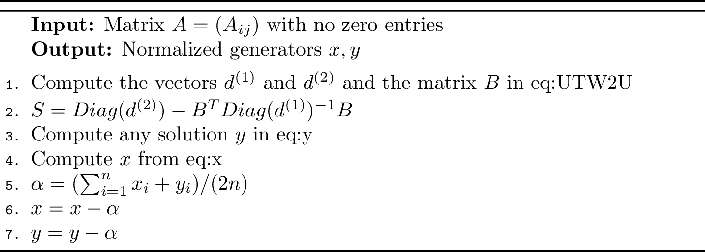
The matrix \(W\) is nonsingular, due to the hypothesis \(A_{ij} \neq 0\), and a unit vector in the kernel of \(U\) is \(v = \mathbf{1}/\sqrt{2n}\). So the formula for the normalized solution of 10 is \[\begin{bmatrix} x \\ y \end{bmatrix} = \bigg[ U^TW^2U + \frac{1}{2n} \mathbf{1}\mathbf{1}^T \bigg]^{-1}U^T W \mathbf{1}.\] Equivalently, the unknown parameters can be recovered from the solution of the linear system \[\label{eq:normaleq} \bigg[ U^TW^2U + \frac{1}{2n} \mathbf{1}\mathbf{1}^T \bigg] \begin{bmatrix} x \\ y \end{bmatrix} = U^T W \mathbf{1}.\tag{11}\] The right-hand side of the linear system is \[U^T W \mathbf{1}= \begin{pmatrix} b^{(1)} \\ b^{(2)} \end{pmatrix}\] with \[b^{(1)}_{i} = \sum_{j=1}^n A_{ij} \qquad b^{(2)}_{i} = \sum_{j=1}^n A_{ji} .\] The matrix \(U^TW^2U\) has the \(2\times 2\) block form \[\label{eq:UTW2U} U^TW^2U = \begin{pmatrix} \mathrm{Diag}(d^{(1)}) & -B \\ -B^T & \mathrm{Diag}(d^{(2)}) \end{pmatrix} ,\tag{12}\] where \(B\) is the entrywise square of \(A\), that is, \(B_{ij} = A_{ij}^2\), and for \(i = 1,\ldots,n\) \[d^{(1)}_{i} = \sum_{j=1}^n A_{ij}^2 \qquad d^{(2)}_{i} = \sum_{j=1}^n A_{ji}^2 .\] The solution of 10 or 11 generally has \(O(n^3)\) computational cost. We can reduce the problem of solving 11 to that of the solution of an \(n\times n\) linear system. First observe that, since the matrix \(U^T W^2 U\) has rank \(2n-1\) and \(U^T W^2 U\mathbf{1}=0\), then all the solutions of 11 are \([x; y]+\gamma \mathbf{1}\), where \([x; y]\) is any solution and \(\gamma\) is an arbitrary constant. However, the generators \(x\) and \(y\) are normalized exactly when the vector \([x;y]\) has zero sum. Therefore, we look for the solution \([x ; y]\) such that \(\mathbf{1}^T [x; y]=0\), so that we solve the system \[\label{eq:UTW2Usystem} U^T W^2 U \begin{bmatrix} x \\ y \end{bmatrix}= U^T W \mathbf{1}.\tag{13}\] From the block structure 12 , by applying one step of block Gaussian elimination, we find that 13 is equivalent to \[\begin{pmatrix} \operatorname{Diag}(d^{(1)}) & -B\\ 0 & S \end{pmatrix} \begin{bmatrix} x \\ y \end{bmatrix} = \begin{pmatrix} I & 0 \\ B^T \operatorname{Diag}(d^{(1)})^{-1} & I \end{pmatrix} \begin{bmatrix} b^{(1)} \\ -b^{(2)} \end{bmatrix},\] where \(S=\operatorname{Diag}(d^{(2)})-B^T \operatorname{Diag}(d^{(1)})^{-1} B\), that is equivalent to the following equations \[\begin{align} x &= \operatorname{Diag}(d^{(1)})^{-1}( b^{(1)} + By),\tag{14} \\ S y & = B^T \operatorname{Diag}(d^{(1)})^{-1} b^{(1)} - b^{(2)}.\tag{15} \end{align}\] The matrix of the latter system is a singular M-matrix, such that \(S\mathbf{1}=0\). From the property \((S-\frac{1}{n}\mathbf{1}\mathbf{1}^T)^{-1}S=I-\frac{1}{n}\mathbf{1}\mathbf{1}^T\), we deduce that the general solution of 15 is \[y=\left(S-\frac{1}{n}\mathbf{1}\mathbf{1}^T\right)^{-1} c+ \gamma \mathbf{1},\] where \(c= B^T \operatorname{Diag}(d^{(1)})^{-1} b^{(1)} + b^{(2)}\) and \(\gamma\) is an arbitrary constant. Another approach to solve 15 consists in considering the \((n-1)\times (n-1)\) nonsingular linear system \(\hat{S} \hat{y}=\hat{c}\), where \(\hat{S}\) is obtained by removing the last row and the last column of \(S\) and \(\hat{c}\) is obtained by removing the last entry of the right-hand side \(c\). Then the vector \(y=[\hat{y}; 0]\) is a particular solution of 15 and all the solutions are \(y+\gamma \mathbf{1}\), with arbitrary \(\gamma\).

Once a solution \(y\) of 15 is computed, the vector \(x\) can be recovered from 14 . Altogether, the solution of 10 can be computed at the cost of \(O(n^3)\) arithmetic operations. The resulting procedure is shown in Algorithm 4.

6 Numerical experiments↩︎

For numerical tests, we implemented Algorithms 1—4 in MATLAB. In Algorithm 4, eq. 15 was solved by applying the backslash operator to the linear system \(\left(S-\frac{1}{n}\mathbf{1}\mathbf{1}^T\right)y=c\). The experiments were run in MATLAB R2024b on a Dell XPS 13 9340 laptop equipped with an Intel Core Ultra 7 155H processor and \(32\) GB of RAM, running Ubuntu 24.04.2 LTS.

We choose a set of uniformly spaced and interlaced Cauchy points, \(x_i = i/n\) and \(y_i = x_i + 1/(2n)\) for \(i = 1,\ldots,n\), and set \(C = \mathop{\mathrm{\tt Cauchy}}(x,y)\). This configuration emphasizes the performance differences among the algorithms. Firstly, we set \(n = 100\). For several noise levels \(\delta\in[10^{-9},10^{-1}]\) we apply a multiplicative componentwise perturbation to \(C\): \[A_{i,j}=(1\pm\delta)C_{i,j}\] where the sign in the perturbation factor is chosen uniformly at random. The same sign pattern is used for all values of \(\delta\). This construction allows us to consider \(\delta\) as a precise estimate of \(\beta_{\max}(A)\), since the absolute value of every entry of the matrix \(\nabla_{x,y}(A) - \mathbf{1}\mathbf{1}^T\) is \(\delta\).

We then apply Algorithms 1–4 to \(A\) and compute Cauchy matrices \(C_1\), \(C_2\), \(C_3\), \(C_4\) from the Cauchy points obtained from the algorithms in the previous sections. For Algorithm 3, vectors \(v\) and \(w\) are chosen such that \(v_j=w_j=2(n-j+1)/n(n+1)\), i.e., entries are positive, uniformly decreasing and have unit sum.

Figure 5 shows the relative normwise errors \(\|C-C_i\|_\mathrm{F}/\|C\|_\mathrm{F}\) (left panel) and \(\|A-C_i\|_\mathrm{F}/\|A\|_\mathrm{F}\) (right panel). They visually appear to be very close to each other. Algorithm 4 provides the best approximation quality in this example by several orders of magnitude, while Algorithm 1 is the least accurate. The dotted line in the figure shows \(\beta_{\max}(A)\), that is \(\delta\). This information is included in relation to Theorem 1, since \(\beta_{\max}(A)\) is a lower bound for the constant \(\beta\) appearing in that theorem. Remarkably, Algorithm 4 produces errors that are below this value.

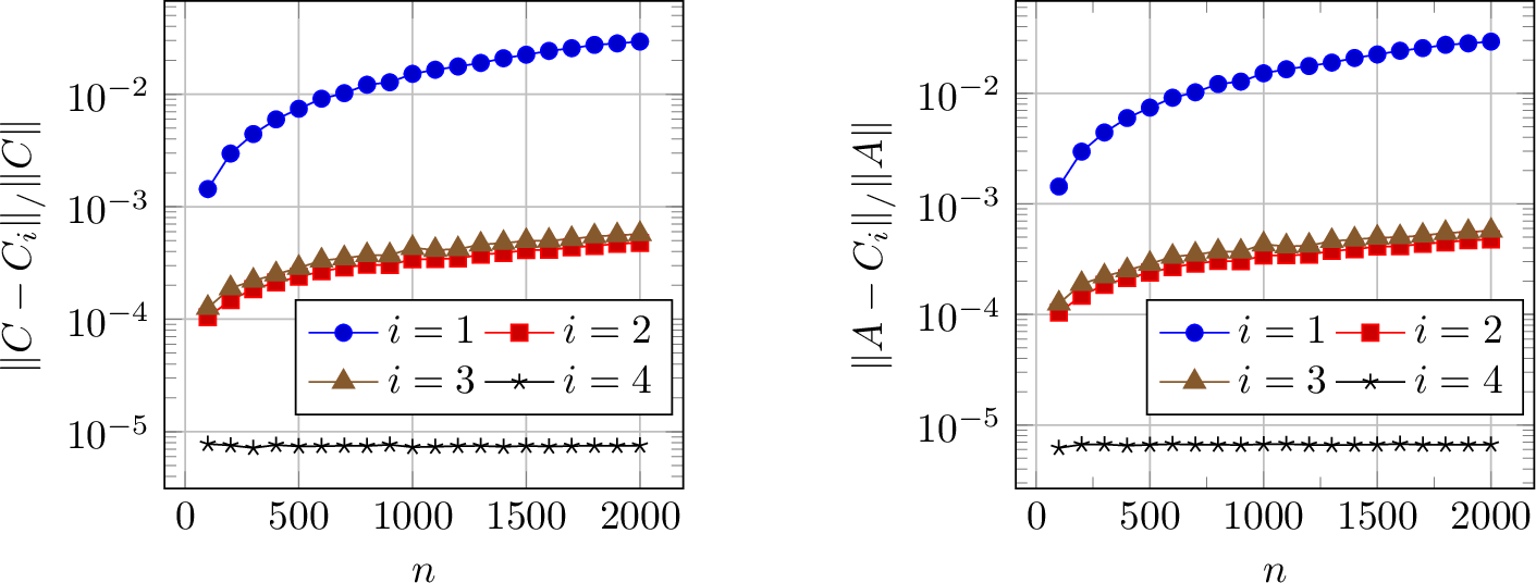
We also compare the performances of Algorithms 1–4 on matrices of increasing size. Here \(\delta=10^{-5}\) is fixed, and matrix size increases from \(100\) to \(2000\). Figure 6 shows relative normwise errors for the four algorithms. As in the previous case, Algorithm 4 yields the best approximation quality; moreover, in contrast to the other algorithms, the relative approximation errors are quite insensitive to \(n\).

This experiment aims to illustrate the validity of a bound from Theorem 4. We generate Cauchy points as in Example 1 with \(n=100\). For several noise levels \(\delta\in[10^{-9},10^{-1}]\) we apply an additive componentwise perturbation to \(D = \Delta(x,y)\), that is, we set \(Z_{ij} = D_{ij} \pm \delta\), where the sign in the perturbation is chosen uniformly at random. The same sign pattern is used for all values of \(\delta\). Then we set \(A = {Z}^{[-1]}\). This construction allows us to consider \(\delta\) as a precise estimate of \(\kappa_{\max}(A)\), since the absolute value of every entry of the matrix \({A}^{[-1]} - D\) is \(\delta\).

For \(i = 1,\ldots,4\), we denote \(C_i\) the Cauchy matrices from the Cauchy points computed by Algorithm \(i\). Figure 7 shows the approximation errors \(\|A-C_i\|_{\mathrm{F}}/\|C_i\|_{\mathrm{F}}\) (left panel) and \(\|A-C_i\|_{\max}/\|C_i\|_{\max}\) (right panel). The dotted line represents the quantity \(4\kappa_{\max}(A)\|A\|_{\max}\), which is the approximation error bound in Theorem 4. The ‘Cauchyness’ criterion employed by Algorithm 4 appears to be more effective at recovering an approximation of the original matrix than the other algorithms. By contrast, Algorithm 1 produces the worst approximation, with an error that nearly reaches the upper bound.

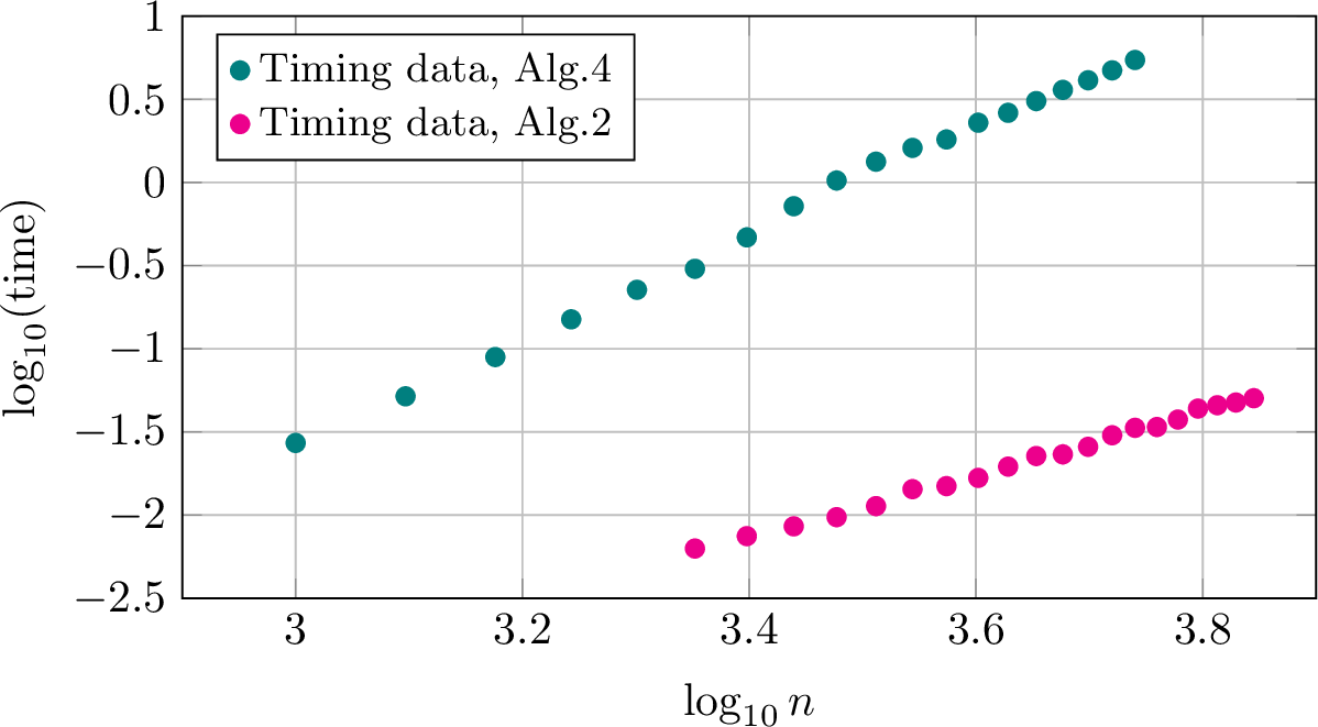
As pointed out at the end of Section 5, a complexity analysis for Algorithm 4 gives an asymptotic computational cost of \(O(n^3)\) arithmetic operations. The analogous cost for Algorithm 2 is \(O(n^2)\), due to the matrix-vector products in the algorithm. In this example, we perform a timing test for Algorithms 2 and 4 with \(n\) ranging from \(500\) to \(5000\). For each matrix size, we compute the average time of ten runs. Then we fit the observed execution times to power laws of the form \(cn^\alpha\) using linear regressions on a log-log scale. The results are shown in Figure 8. The exponents computed by linear regressions closely match the theoretical values.

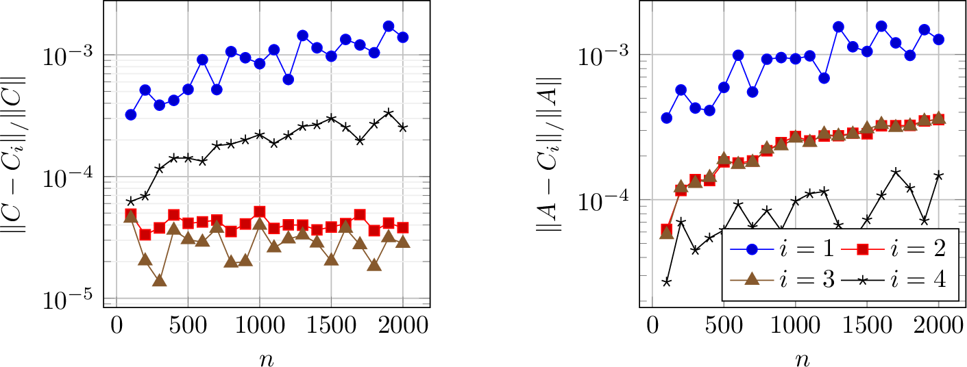
In Example 1, the perturbation is evenly spread across the test matrix. It is therefore understandable that Algorithm 2 works slightly better than Algorithm 3 applied with uniformly decreasing vectors \(v\) and \(w\). On a matrix where the perturbation mainly affects the trailing principal block, we expect the opposite behavior. To verify this conjecture numerically, we set up test data as in the second part of Example 1, except that the perturbation applied to entry \((i,j)\) is weighted by a factor \(n/(n-i+1)(n-j+1)\). Figure 9 shows that Algorithm 3 does indeed provide the best reconstruction of the original Cauchy matrix. However, the best approximation to \(A\) is given by Algorithm 4.

In this example, we focus on errors for componentwise inverses of Cauchy matrices. Recall that Theorem 4 provides an upper bound for such errors, which depends on the norm of the projection operator associated with the chosen algorithm. From the proof of Theorem 4, one may also pinpoint worst-case perturbations that make the bound sharp (i.e., equality is attained). Such perturbations can be chosen as scalar multiples of the matrix obtained from a square columnwise reshape of the dominant right singular vector of the operator \(M_w\otimes M_v\). For instance, for the operator \(M_{e_1}\otimes M_{e_1}\) associated with Algorithm 1 such a worst-case perturbation is the \(n\times n\) matrix \(Y = vv^T/v^Tv\) where \(v = (1,-1/(n-1),\ldots,-1/(n-1))^T\in{\mathbb{R}}^n\) is the right singular vector of \(M_{e_1}\) associated with the dominant singular value, \(\|M_{e_1}\|_2 = \sqrt{n}\). Hence, \[\begin{align} Y(1,1)&=\frac{n-1}{n},\\ Y(1,i)&=Y(i,1)=-\frac{1}{n},\qquad & i=2,\ldots n,\\ Y(i,j)&= \frac{1}{n(n-1)}, & i,j=2,\ldots,n. \end{align}\] Notably, this matrix is orthogonal to \(\mathcal{D}\) with respect to the Frobenius inner product. This can be verified by computing the projection of \(Y\) onto \(\mathcal{D}\), using the projector \(\Phi_2\) in Theorem 3. The projection is zero, as \(\mathbf{1}^Tv = 0\). Consequently, if \(A\) is any matrix such that \({A}^{[-1]} = D + \delta Y\) for some \(\delta\geq 0\) and \(D\in\mathcal{D}\) then \(\kappa_\mathrm{F}(A) = \delta\). Moreover, if \(D_1\in\mathcal{D}\) denotes the matrix recovered by Algorithm 1 then \(\|{A}^{[-1]} - D_1\|_\mathrm{F}= \|M_{e_1}\|_2^2\, \kappa_\mathrm{F}(A) = n\delta\), that is, we have equality in Theorem 3.

For \(n\) ranging from \(100\) to \(2000\) we define a Cauchy matrix \(C\) as in Example 1, compute its componentwise inverse \(D\) and consider the perturbed matrix \(Z=D+\delta Y\), with \(\delta=10^{-5}\). Algorithms 1–4 are applied to \(A=Z^{[-1]}\), and we recover matrices \(D_i\in\mathcal{D}\) and \(C_i = {D_i}^{[-1]}\) for \(i=1, 2, 3, 4\). The left panel in Figure 10 shows errors \(\|Z-D_i\|_\mathrm{F}\). In accordance with Theorem 4 we expect \(\|Z-D_1\|_\mathrm{F}= n\delta\) and \(\|Z-D_2\|_\mathrm{F}= \delta\), as it actually occurs numerically. The relative errors \(\|A-C_i\|_\mathrm{F}/\|A\|_\mathrm{F}\) shown in the right panel increase as \(O(n)\), corresponding to the growth of \(\|A\|_{\max}\). Also in this example, the results of Algorithms 2 and 3 are almost indistinguishable, while Algorithm 4 provides the best approximation to \(A\), but not to \(C\).

Acknowledgements↩︎

This work was partially supported by the Italian Ministry of University and Research (MUR) through the PRIN 2022 “Low-rank Structures and Numerical Methods in Matrix and Tensor Computations and their Application” code 20227PCCKZ MUR D.D. financing decree n. of February 2nd, 2022 (CUP I53D23002280006 and CUP E53D23005520006), and through the MUR Excellence Department Project awarded to the Department of Mathematics, University of Pisa, CUP I57G22000700001. The authors are also affiliated to the INdAM-GNCS (Gruppo Nazionale di Calcolo Scientifico).

7 A different parametrization of \({\mathcal{D}}\)↩︎

Let \({\mathbb{R}}^n_0\) denote the set of zero-sum vectors in \({\mathbb{R}}^n\): \[{\mathbb{R}}^n_0 = \{x\in{\mathbb{R}}^n: \mathbf{1}^T x = 0\} .\] The matrix space \(\mathcal{D}\) introduced in 2 admits the following alternative description: \[\mathcal{D} = \{\hat{x}\mathbf{1}^T + \mathbf{1}\hat{y}^T + \alpha \mathbf{1}\mathbf{1}^T: \hat{x},\hat{y}\in {\mathbb{R}}^n_0,\;\alpha\in{\mathbb{R}}\} .\] More precisely, every matrix \(D\in\mathcal{D}\) can be written in a unique way as \[\label{eq:ourdecomp} D = \hat{x}\mathbf{1}^T + \mathbf{1}\hat{y}^T + \alpha \mathbf{1}\mathbf{1}^T\tag{16}\] for some \(\hat{x},\hat{y}\in {\mathbb{R}}^n_0\) and \(\alpha\in{\mathbb{R}}\). It is interesting to study the properties of this decomposition, which differs from the one using normalized generators introduced in [5] and recalled in Section 2. Notably, the three terms in the right-hand side of 16 are mutually orthogonal for the Frobenius inner product. Henceforth, for any \(D\in{\mathcal{D}}\) let \(\mathcal{R}(D)\) be the vector \([\hat{x}; \hat{y}; \sqrt{n}\alpha]\in{\mathbb{R}}^{2n+1}\) identified by 16 . We immediately obtain that \(\|D\|_\mathrm{F}= \sqrt{n}\|\mathcal{R}(D)\|_2\). Indeed, the orthogonality of the three terms in 16 gives \[\|D\|_\mathrm{F}^2 = \|\hat{x}\mathbf{1}^T\|_\mathrm{F}^2 + \|\mathbf{1}\hat{y}^T\|_\mathrm{F}^2 + \|\alpha \mathbf{1}\mathbf{1}^T\|_\mathrm{F}^2 = n \big( \|\hat{x}\|_2^2 + \|\hat{y}\|_2^2 +n\alpha^2 \big) = n \|\mathcal{R}(D)\|_2^2 .\] Thus, apart of the factor \(\sqrt{n}\), the map \(\mathcal{R}\) is an isometric bijection between the metric space \(({\mathcal{D}},\|\cdot\|_\mathrm{F})\) and the subspace \({\mathbb{R}}^n_0\times{\mathbb{R}}^n_0\times{\mathbb{R}}\) of \({\mathbb{R}}^{2n+1}\) endowed with the \(2\)-norm. As such, it produces a perfectly well conditioned representation of matrices in \({\mathcal{D}}\). This motivates us to evaluate the conditioning of the representation provided by normalized generators, as shown below.

The following result is analogous to Theorem 3.6 in [5] (restricted to square matrices) but pertains to the representation 16 instead of the one with normalized generators. Our representation is shown to have a tighter error bound than the other one when recovering a perturbed Cauchy matrix via Algorithm 2.

References↩︎