Modeling Globular Cluster Stellar Streams with a Basis-Expansion \(N\)-body Code
February 13, 2026
Abstract
Globular cluster stellar streams probe galaxy-formation processes and can potentially reveal the distribution of dark matter in galaxies. In many theoretical studies, streams are modeled with particle-spray or direct \(N\)-body codes. But particle-spray methods abstract away the internal dynamics of the progenitor by making strong assumptions about the escape physics, while direct \(N\)-body is prohibitively
expensive for realistic (\(N\!>\!10^5\)) systems. In this paper, we present the stream-modeling capabilities of KRIOS, a new basis-expansion \(N\)-body code for collisional stellar
dynamics, that bridges this runtime vs. accuracy gap. We show that KRIOSreproduces NBODY6++GPUcluster models, and their associated streams, more accurately than particle spray in a fraction of the NBODY6++GPUwall-clock time. We
then compare KRIOSto various particle-spray methods on 10 orbits similar to known Milky Way streams. The morphology and kinematics of these streams most disagree when the progenitor is tightly bound to the host, as these systems are often subject to
stronger tidal forces. Finally, we discuss which elements of the progenitor physics are most important for modeling stellar streams and how these might be incorporated into particle-spray methods.
1 Introduction↩︎
There are lingering discrepancies between Local-Group-scale \(\Lambda\)CDM predictions and observations [1] that near-field cosmologists are eager to rectify. The Milky Way (MW) and its population of globular clusters (GCs) could provide key insight into these tensions. GCs can either form in situ as a mode of star formation in galaxies, or can be accreted from other galaxies during mergers [2], [3]. Both formation channels can help constrain the MW’s formation history [2], [4]–[6]. Conversely, the host environment of the MW plays a key role in the dynamical evolution of its GCs. As the Galactic potential changes along a cluster’s orbit, the loss of stars to the tidal field can significantly accelerate the destruction of Galactic GCs [7]. These lost stars go on to create debris such as stellar streams [8] or shells [9], which probe the Galactic potential. Accurate, long-term models of GC evolution that include interactions with their host galaxy [10] would thus improve both galaxy-formation [11], [12] and GC studies.
![Figure 1: A model produced by the KRIOShybrid N-body code (Orbit 3, Table 1), where we see both stream-like and shell-like features at {t\!=\!5\,{\rm Gyr}}. The unbound particles are color coded by their energy with respect to the host E, which is mostly conserved for escapers modulo small perturbations from the cluster potential. The bound particles (Section 2.2) are shown in black. Top panel: The stream shown in the MW’s reference frame, with a bulge and disk added for illustrative purposes. Bottom panel: The stream shown in the great-circle reference frame for an observer stationed at the Galactic center. The angle \phi_{1} subtends an element of the stream track and \phi_{2} subtends the angle out of the progenitor’s instantaneous orbital plane (see Figure 2 for the axis definitions). The stream progenitor (i.e., the cluster) is at {\phi_{1}\!=\!\phi_{2}\!=\!0^{\circ}}. Both the leading (blue) and trailing (red) tails contain epicyclic density fluctuations [13] and energy feathering [14], both well-known features of streams in axisymmetric potentials [15]. The density fluctuations are most clear near the progenitor; see Figure 9 for a direct comparison.](/article/2602.13385/combined_snapshot_panels.png "fig:")
The dynamically cold streams from GCs, in particular, are highly sensitive to perturbations from substructure within the host galaxy [15], including both baryonic substructure [16], [17] and dark matter subhalos [18]–[20]. The presence of dark subhalos, which are clumps of dark matter too small to form stars, in galaxies is a key prediction of \(\Lambda\)CDM and a potential clue to the nature of dark matter itself [1], [21]. Several GC streams in the MW, including the GD-1 stream [22], display features that may have been the result of an encounter with a subhalo [23]. The kinematic temperature of GC streams is also thought to depend on the subhalo mass-concentration relation [24]–[26]. However, substructure in GC streams can also be the result of the GC progenitor’s properties and internal evolution [27], interactions with baryonic substructure in the host galaxy, or larger perturbations in the host potential itself [28], [29]. Distinguishing which features of a stream are caused by its progenitor from those caused by the baryonic or DM substructure of the host galaxy is crucial to successfully probing dark matter physics with stellar streams.
The first approach for modeling dense GCs is often a direct \(N\)-body integration, where the forces between pairs of stars are directly summed every timestep. The gold standard for this is the
NBODY6++GPUcode [30], [31]. A variation of the same code allows the GC to be
coupled to an external tidal field as well [32], following both the progenitor and resultant stream self-consistently within a time-independent host
potential. But the direct summation of forces required to solve \(N\) coupled ordinary differential equations (ODEs) requires \(\mathcal{O}(N^{2})\) operations, making this technique
computationally expensive. Despite significant algorithmic enhancements (e.g., regularization of close encounters and block timesteps) and hardware acceleration (e.g., GPUs), direct summation still has not been used to model a GC with a density and
initial \(N\) typical of Galactic GCs over a full Hubble time. Direct \(N\)-body methods are thus ill-suited to generating the large grids of model streams necessary to explore the dynamics
within and external to GCs that affect stream properties relevant to probing Galactic substructure.
To hasten computation, stream models rely on more approximate methods. Particle-spray codes [33]–[39] generate stream models far more rapidly than direct \(N\)-body by approximating the escape process, directly injecting stars near the Lagrange points of the GCs as they orbit their host. For example, [35] and [38] sample the rate and kinematic properties of escaping stars from distributions tuned to mimic \(N\)-body simulations of tidal disruption [40]–[42]. While these methods excel in generating large ensembles of models, they assume that the details of the tidal-stripping process do not substantially affect stream properties such as its density and velocity dispersion profiles. Furthermore, most particle-spray studies in the literature have assumed a fixed progenitor [37], [43] or no progenitor at all [44], [45], both of which limit their ability to resolve realistic stream production over long timescales where the cluster has a time-dependent size and mass.
What is needed is an approach that can accurately model an evolving, collisional GC and its ejecta in a fraction of the direct \(N\)-body wall-clock time. In numerical studies of GCs, this is often done with Monte Carlo
methods, where the collisional evolution of dense star clusters can be approximated by statistical techniques. Leading codes in this area include MOCCA [46] and CMC[47], both of which use the [48] method to approximate two-body relaxation [49] via effective “super-encounters” with a
nearby neighbor. The Hénon method scales as \(\mathcal{O}(N\log N)\), satisfying the need for star-by-star GC simulations with \(\mathcal{O}(<\!N^{2})\) complexity that can capture the
cluster’s gravothermal evolution and conserve the integrals of motion. As an example, [50] showed that CMCproduces models with \({N\!=\!10^{6}}\) that agree with NBODY6++GPUon important structural and stellar population properties in about a day; by comparison, the same cluster model integrated with NBODY6++GPUrequired
approximately six months of wall-clock time wang2016?.
However, Hénon-style Monte Carlo codes like CMCassume that the cluster is spherically symmetric, with all the relevant dynamical processes occurring on a relaxation timescale [47]. In reality, the tidal force is anisotropic in the cluster reference frame and can do work on the cluster on a dynamical timescale. Stars ejected at low energies can only escape through
openings in the zero-velocity surface near the \(L_{1}\)/\(L_{2}\) Lagrange points, even after the star has become energetically unbound from the system. As such, it typically requires many
dynamical times for a star to actually exit the cluster [51], [52]. To
account for this, most Monte Carlo codes adopt prescriptions that approximate the tidal radius of the cluster [53], [54] and introduce delays to the stripping of particles from the system [46], [55]. These prescriptions must be tuned to direct \(N\)-body simulations of clusters on specific orbits, and are not necessarily reliable for other orbits in a
different, or time-varying, host potential. Furthermore, because escapers have to be removed from CMCand its spherical collisional dynamics before evolving their orbits (collisionlessly) in a realistic asymmetric tidal field, these Monte Carlo
methods require significant post-processing to model tidal debris in a Galactic context [27], [52], [56].
This combination of requirements has motivated the development of KRIOS, a new \(N\)-body code introduced by [57]. Figure 1 provides an illustrative KRIOSmodel of a GC stellar stream in a MW-like host potential. KRIOSintegrates each particle in a self-consistent gravitational field [58]–[63] that adapts as the cluster evolves , while two-body relaxation is modeled using a 3D version of Hénon’s original effective encounters. The force calculations are \(\mathcal{O}(N)\) and parallelizable, rendering complete forward models considerably faster than direct \(N\)-body methods. KRIOSreplicates key dynamical properties of non-rotating clusters (such as core collapse in clusters with varying levels of initial velocity anisotropy), as well as rotating clusters (such as the collisional evolution of a cluster’s rotation curve, and the emergence of the radial orbit instability in highly anisotropic clusters). See for details. Because KRIOSintegrates the stellar orbits in a non-spherical cluster on a dynamical timescale, it is well suited to exploring the production of tidal debris from disrupting star clusters in a fraction of the direct \(N\)-body wall-clock time.
In Section 2, we introduce the scaffolding that helps KRIOSresolve mass loss due to external tidal fields. In Section 3, we show comparisons between the streams produced by KRIOSand
NBODY6++GPUto validate our method, as well as comparisons to various particle-spray methods, in order to explore the regions of Galactic orbital space where the reliability of the latter breaks down. The discussion (Section 4) highlights the benefits of using KRIOSdesign elements in modeling stellar streams, and describes key features relevant to future particle-spray studies
2 Methods↩︎
KRIOSdecomposes the gravitational interactions in a star cluster into collisionless and collisional components. The collisionless gravitational potential is modeled by expanding the cluster’s mass density with a set of basis functions: \[\begin{align} \tag{1} \psi_{\rm SCF}(\boldsymbol{r}) &= \sum_{n\ell m} a_{n \ell m} \, \psi^{(n\ell m)}(\boldsymbol{r}), \\ \tag{2} \rho_{\rm SCF}(\boldsymbol{r}) &= \sum_{n\ell m} a_{n \ell m} \, \rho^{(n\ell m)}(\boldsymbol{r}). \end{align}\] The basis functions are separable in spherical coordinates: \[\begin{align} \label{eq:psi95nlm} \psi^{(n\ell m)}(\boldsymbol{r}) &= U_{n}^{\ell}(r)\,Y_{\ell}^{m}(\theta, \phi), \\ \rho^{(n\ell m)}(\boldsymbol{r}) &= D_{n}^{\ell}(r)\,Y_{\ell}^{m}(\theta,\phi), \end{align}\tag{3}\]
where \({n,\,\ell}\) index the radial basis functions \({\{U_{n}^{\ell}(r), D_{n}^{\ell}(r)\}}\) and \({\ell,\,m}\) index the spherical harmonics \(Y_{\ell}^{m}(\theta,\phi)\). In the standard self-consistent field approach, \(\psi^{(n\ell m)}\) and \(\rho^{(n\ell m)}\) are bi-orthogonal sets where each mode constitutes an independent solution to Poisson’s equation such that \({\nabla^{2}\psi^{(n\ell m)}\!=\!4\pi G \, \rho^{(n\ell m)}}\). The bi-orthogonality relation can be used to isolate each basis coefficient \(a_{n\ell m}\):
\[\begin{align} a_{n \ell m} &= -\int {\rm d}\boldsymbol{r} \,\rho(\boldsymbol{r}) \, \psi^{\star(n\ell m)}(\boldsymbol{r}),\\ &\simeq -\sum_k \,m_k \, \psi^{\star(n\ell m)}(\boldsymbol{r}_k), \label{eqn:sumanlm} \end{align}\tag{4}\]
where \(\psi^{(n\ell m)\star}\) is the complex conjugate of \(\psi^{(n\ell m)}\) and we have estimated the cluster’s mass density from the particle data as \({\rho(\boldsymbol{r}) \!\simeq\! \sum_{k} m_{k} \, \delta^{3}(\boldsymbol{r}-\boldsymbol{r}_{k})}\).
The individual stars are then integrated forward in the global \(\psi_{\rm SCF}(\boldsymbol{r})\) potential. This reduces the \(N^2\) calculation of direct \(N\)-body to \(N\) individual, embarrassingly parallel integrations. In general, the greatest computational bottleneck for the SCF method is the large number of modes that are required when the basis functions are not well fit to the cluster’s mass density [59]. To address this, KRIOSuses a tunable set of basis functions from [60], where the zeroth-order mode of the potential has the following functional form:
\[U_{0}^{0}(r)\!\propto\!\frac{1}{\left(1+\left(\frac{r}{b}\right)^{1/\alpha}\right)^{\alpha}}, \label{eqn:u00}\tag{5}\]
. KRIOStunes the exponent \(\alpha\) and scale length \(b\) such that the true cluster potential is well approximated by the zeroth-order mode of the SCF even as the density profile becomes cuspy near core collapse . This, combined with a filtering procedure that ignores modes where \({a_{n\ell m}\ll a_{000}}\), allows KRIOSto maintain an optimized description of the cluster potential over many relaxation times. See Section 2.2 of for details.
Finally, KRIOSmodels the relaxation of star clusters with the [48] prescription, where the cumulative effect of many two-body encounters are modeled as a single effective “super-encounter” between a star and a suitably chosen neighbor. We approximate the local number density of particles, a key ingredient for computing the relaxation timescale [47], using \({n_{\rm neigh}\!=\!30}\) neighbors. We then update each particle’s 3D velocity based on the relevant two-body super-encounter at each system timestep. These scattering events diffuse energy from the cluster’s core to its halo, and have been shown to reproduce the expected gravothermal evolution and core collapse of star clusters over many relaxation times; see . Note that we do not apply the energy conservation scheme from [64] in this study. This scheme is often used to correct the energy drift observed in Monte Carlo codes [47] that arises from sampling new orbital positions and velocities (post two-body relaxation) in the old cluster potential from the previous timestep. In this study, however, the cluster potential is updated much more frequently (see Section 2.2). As a result, our models conserve energy in the host frame of the Galaxy \(E\) (\(\Delta E/E_0\lesssim 10^{-3}\)) and the \(z'\) component of the angular momentum \(L_{z'}\) (\(\Delta L_{z'}/L_{z',0}\lesssim 10^{-2}\)) at acceptable levels over the 5 Gyr integrations presented here.
2.1 KRIOSReference Frames↩︎
KRIOSuses accelerating, non-rotating reference frames for the SCF, which mitigates the need to include rotational pseudo-forces into the equations of motion explicitly [65]. Our framework is illustrated in Figure 2. For a static host potential, we set the fixed inertial frame to coincide with the center of the bulge, disk, and dark matter halo components (the primed coordinates in Figure 2).

KRIOShas separate reference frames for the host potential and the cluster. The position of the cluster frame (unprimed coordinates, Figure 2) is set to the location that maximizes the \(a_{000}\) component of the basis expansion (using a similar procedure for finding the optimal \(\alpha\) and \(b\) in Equation 5 ). Because the SCF basis does not contain any information about the velocity of the system, the velocity for the reference frame is determined by taking a mass-weighted average of the particle velocities in the cluster’s core, where \({r_{\rm core} \!=\! \sqrt{\sum_{i} \rho_{\rm SCF}^{2}(\boldsymbol{r}_{i}) r_{i}^{2} / \sum_{i}\rho_{\rm SCF}^{2}(\boldsymbol{r}_{i})}}\).1
In order to return accurate solutions to each particle’s equations of motion, the ODE solver must be able to determine each particle’s location with respect to both the SCF and host at arbitrary times during each integration (purple segments in Figure 2). As such, each star must have access to the position of the cluster at arbitrary times along its orbit. To that end, we integrate a test particle—located at the cluster’s center of mass2—in the host potential, and collect position and velocity samples along that orbit. These samples are then used to create a quintic Hermite spline [66], [67], to determine the position of the cluster at arbitrary times. Each star can then be integrated forward in the host reference frame individually, without the need to synchronize the center of the cluster after every individual particle integration step.
2.2 Cluster Timescales in an External Potential↩︎
For the collisional models in , the KRIOSsystem timestep was chosen to be a fraction of the relaxation time of the cluster. After the particles were integrated forward in the potential, we performed two-body relaxation and updated the SCF potential using the new positions of the particles, on the assumption that the potential of the cluster could only change significantly on a relaxation timescale. However, for clusters in realistic tidal fields, the associated mass loss can occur faster than the typical relaxation timescale in the core. Furthermore, the external potential of the host can do work on the cluster on a dynamical timescale, e.g. compressive shocks from the Galactic disk [49] and during perigalacticon passages like \(\boldsymbol{r}_{\rm cluster}'(t_{2})\) in Figure 2. To resolve this, we introduce separate timesteps for performing two-body relaxation and updating the cluster potential:
The system timestep, \(\Delta t_{\rm sys}\), where we perform two-body relaxation and completely recompute the cluster SCF, as in Equation (14) of .
The integration timestep, \(\Delta t_{\rm int}\), where we update the SCF potential on a timescale set by the changing tidal field experienced by the cluster.
To calculate \(\Delta t_{\rm int}\), we evaluate the tidal tensor (\(\boldsymbol{T}\), the Hessian of the potential) at every point along the orbit of the cluster test particle described in Section 2.1. Following [68], we define the integration timestep as
\[\Delta t_{\rm int} = \sqrt{\eta}~\left({1\over 6}||\boldsymbol{T}(\boldsymbol{r}'(t))||^{2}\right)^{-1/4}, \label{eq:tidal95timestep}\tag{6}\]
where \(||\cdot||\) is the Frobenius norm of the tidal tensor, computed with respect to the primed coordinates,
\[T_{ij}(\boldsymbol{r}'(t))= \left(-\partial_{x_{i}'}\partial_{x_{j}'}\, \psi_{\rm host}\right)\Big|_{\boldsymbol{r}'=\boldsymbol{r}'(t)}, \label{eq:tidal95tensor}\tag{7}\]
and \(\eta\) is a free parameter (\({\eta\!=\!1/400}\) in this study, chosen from the values discussed in [68] after validation tests). This allows KRIOSto resolve changes to the cluster mass and potential that occur faster than the two-body relaxation timescale. KRIOSevaluates Equation 7 directly from the various host potential components; see Appendix 6.
KRIOSupdates the SCF in two ways: “complete" refreshes, where \(\alpha\) and \(b\) in Equation eq. ¿eq:eqn:u00? are retuned and the SCF is reevaluated from scratch, and”intermediate" refreshes, where only particles that have become unbound from (or been recaptured by) the cluster are subtracted from (or added to) \(a_{n \ell m}\) via the sum in Equation 4 . In this study, KRIOSexecutes a complete SCF refresh every 5 integration timesteps. We use an energy-based analog to the Lagrange radii, i.e., \(r_{x}\) is the smallest radius that encloses \(x\%\) of the energetically-bound particles3, to determine which particles are included in the Equation 4 calculation. We only include particles where \({r \!\leq\! r_{99.9}}\) and refer to \(r_{100}\), the smallest radius that encloses all energetically-bound particles, as the “bound radius" \(r_{b}\).
Finally, the SCF is susceptible to finite-\(N\) noise [59], [62]; this can be reduced by sampling multiple positions along the particles’ orbits during each integration. In , this was done with an equal number of samples per system timestep (based only on the relaxation timescale). As we are interested in changes that can occur on a dynamical timescale, here we collect orbital samples based on the cluster’s instantaneous dynamical time, \[\begin{align} N_{{\rm samples}} &= {\rm max}\left(1, \left\lceil n_{{\rm samples, \,} t_{\rm dyn}} \, \times{\Delta t_{\rm int} \over t_{\rm dyn}}\right\rceil\right), \end{align}\] where \(n_{{\rm samples,} \, t_{\rm dyn}}\) is the desired number of samples per the instantaneous half-mass dynamical time [69], i.e. \[\begin{align} \left({t_{\rm dyn} \over 4.3451 \, {\rm Myr}}\right) = \left({M_{\rm cluster} \over 10^{5} \, M_{\odot}}\right)^{-1/2} \, \left({r_{\rm hm} \over 10 \, {\rm pc}}\right)^{3/2}. \end{align}\] In this study, we set \({n_{{\rm samples,} \, t_{\rm dyn}}\!=\!1}\).
2.3 Sampling Orbits Consistent with MW GCs↩︎
![Figure 3: Top panel: The integrals of motion for the second set of Table 1 orbits compared to the known population of MW GCs [70]–[72] and stellar streams [5]. [73] classifies MWGCs based on extinction A_{V} and background density N_{\rm bg}. Bottom panel: The sampled orbits compared to the MWGCs and streams in the meridional plane, showing that our sample is biased toward orbits in the MW halo. Orbits 3 (closer to {z'\!=\!0}) and 5 are boldened for illustrative purposes, as they are the stream models shown explicitly in Sections 3 and 4.](/article/2602.13385/krios_ii_orbits_with_mw_gcs_2x1.png "fig:")
We must determine a set of orbit initial conditions consistent with the known population of MWGCs [70]–[72], [74] and stellar streams [5], [15], [75] before highlighting the ways in which KRIOSmodels disagree with particle spray. The eccentricity and
inclination are not necessarily conserved for orbits in non-Keplerian potentials, so we use conserved quantities that are readily accessible from observational data instead. Our set of orbits is shown in Figure 3.
Recall that the energy \(E\) and \(z'\)-component of the angular momentum \(L_{z'}\) are integrals of the motion for a test particle in a static and
axisymmetric host potential. The energy can be expressed in terms of the angular momentum and meridional plane coordinates : \[\begin{align}
\label{eq:energy95eff} E &= {1\over 2}(v_{\varrho'}^{2} + v_{z'}^{2}) + \psi_{\rm eff}(\varrho', z'), \\
\psi_{\rm eff}(\varrho', z') &\equiv \psi_{\rm host}(\varrho', z') + {L_{z'}^{2} \over 2\varrho'^{2}}.
\end{align}\tag{8}\] Therefore, if we start with a grid of \({(|L_{z'}|, E)}\) values (Figure 3’s top panel), we can identify nearby MWGCs in that space if we use
MilkyWayPotential2022 [76] to estimate \(\psi_{\rm host}\). We sample the initial
Galactocentric distance of each orbit, \(r_{\rm init}'\), based on the apogalacticon estimates—\(\boldsymbol{r}_{\rm cluster}'(t_{1})\) in Figure 2—for the nearest MWGCs: \({r_{\rm init}'\!\sim\!\mathcal{N}(\mu_{r_{\rm apo}'}, \sigma_{r_{\rm apo}'}^{2})}\). This ensures that the cluster is not subject to substantive
mass loss at the moment of initialization. The phase-space initial conditions, for a given set of \({(L_{z'},E,r_{\rm init}')}\) values, can then be sampled in the following way: \[\begin{align}
\alpha &\sim \mathcal{U}(-\pi/2, \pi/2),\beta \sim \mathcal{U}(0,2\pi) \\
\varrho_{\rm init}' &= r_{\rm init}' \cos\alpha, \\
\varphi_{\rm init}'&\sim\mathcal{U}(0,2\pi), \\
z_{\rm init}' &= r_{\rm init}'\sin\alpha, \\
v_{\varphi', {\rm init}} &= L_{z'} / \varrho_{\rm init}', \\
v_{\varrho', {\rm init}} &= v \cos\beta, \\
v_{z', {\rm init}} &= v\sin\beta,
\end{align}\] where \({v \!\equiv\! \sqrt{2\left(E \!-\! \psi_{\rm eff}(\varrho_{\rm init}', z_{\rm init}')\right)}}\). We only create retrograde orbits [15] for simplification, which is permissible due to the axisymmetry of the host potential. An orbit with \({t_{\rm end} \!=\! 5 \, {\rm Gyr}}\) and timestep \({\Delta t \!=\! 0.1 \, {\rm Myr}}\) is integrated using gala [76] to confirm that \({1 \, {\rm kpc} \!\leq \!r_{\rm peri}'}\) and \({10 \, {\rm kpc} \!\leq\! r_{\rm apo}' \!\leq\! 60 \, {\rm kpc}}\); see the bottom panel of Figure 3. If there are no \({(\varrho',z')}\) pairs that satisfy \({E\!\geq\!\psi_{\rm eff}(\varrho_{\rm init}',z_{\rm init}')}\) and the \({(r_{\rm peri}', \,r_{\rm apo}')}\) constraints, then the \({(|L_{z'}|, E)}\) pair is discarded.
While our method for sampling orbits starts directly from the integrals of motion, it is still useful to describe orbits in terms of their circularity [77] and eccentricity, which can be defined in the following way: \[\begin{align} \varepsilon &\equiv {L_{z'} \over L_{z', {\rm circ}}(E)}, \\ e &\equiv {r_{\rm apo}' - r_{\rm peri}' \over r_{\rm apo}' + r_{\rm peri}'}, \end{align}\] where \({L_{z',{\rm circ}} \!=\! \varrho'\sqrt{2(E \!-\! \psi_{\rm host}(\varrho',0))}}\) and \(\varrho'\) is the radius at which a circular orbit in the disk has energy \(E\). The inclination of the cluster’s orbital plane with respect to the disk, \({\cos i\!=\!L_{z'}/|\boldsymbol{L}|}\), is not necessarily constant for a non-Keplerian potential. The properties of the orbits in Figure 3 can be found in Table 1.
| Orbit ID | \(r_{\rm peri}'\) [kpc] | \(r_{\rm apo}'\) [kpc] | \(t_{\rm last\,peri}\) [Gyr] | \(t_{\rm last\,apo}\) [Gyr] | \(\varepsilon\) | \(e\) | \(i\) [deg] | \(L_{z'}\) [\(10^{3}\) kpc km/s] | \(E\) [\(10^{5}\) (km/s)\(^{2}\)] | |
|---|---|---|---|---|---|---|---|---|---|---|
| Circular 0 Test | 5.00 | 5.00 | – | – | 1.00 | 0.00 | \(0.0\!\pm\!0.0\) | 1.13 | -1.30 | |
| Circular 1 Test | 20.00 | 20.00 | – | – | 1.00 | 0.00 | \(0.0\!\pm\!0.0\) | 3.95 | -0.72 | |
| Eccentric Test | 20.00 | 5.00 | – | – | 0.20 | 0.60 | \(79.27\!\pm\!0.68\) | 0.33 | -0.87 | |
| 0 | 1.55 | 14.25 | 4.87 | 4.95 | 0.10 | 0.80 | \(75.00\!\pm\!3.45\) | 0.20 | -1.24 | |
| 1 | 2.56 | 13.83 | 4.89 | 4.98 | 0.26 | 0.69 | \(60.76\!\pm\!3.68\) | 0.53 | -1.24 | |
| 2 | 3.88 | 25.76 | 4.69 | 4.85 | 0.06 | 0.74 | \(82.87\!\pm\!0.45\) | 0.20 | -0.98 | |
| 3 | 4.10 | 13.20 | 4.83 | 4.91 | 0.91 | 0.53 | \(18.20\!\pm\!3.29\) | 1.41 | -1.24 | |
| 4 | 4.85 | 25.18 | 4.79 | 4.95 | 0.17 | 0.68 | \(73.87\!\pm\!0.70\) | 0.53 | -0.98 | |
| 5 | 9.47 | 22.03 | 4.74 | 4.91 | 0.47 | 0.40 | \(60.63\!\pm\!0.48\) | 1.41 | -0.98 | |
| 6 | 11.72 | 46.87 | 4.59 | 4.92 | 0.09 | 0.60 | \(82.63\!\pm\!0.05\) | 0.53 | -0.72 | |
| 7 | 12.50 | 46.36 | 4.97 | 4.64 | 0.23 | 0.58 | \(70.88\!\pm\!0.11\) | 1.41 | -0.72 | |
| 8 | 18.49 | 41.90 | 4.43 | 4.77 | 0.04 | 0.39 | \(87.86\!\pm\!0.01\) | 0.20 | -0.72 | |
| 9 | 28.68 | 32.88 | 4.90 | 4.56 | 0.61 | 0.07 | \(52.74\!\pm\!0.10\) | 3.76 | -0.72 |
3 Results↩︎
We now run and compare ensembles of KRIOS, NBODY6++GPU, and particle-spray models of stellar streams on several different orbits in our Galaxy. In each ensemble, the stream’s progenitor cluster has an initial mass \({M_{\rm cluster} \!=\! 10^{5} \, M_{\odot}}\) and half-mass radius \({r_{\rm hm}\!=\!10 \, {\rm pc}}\). The progenitor cluster in each KRIOSand NBODY6++GPUsimulation is initialized
with equal-mass point particles sampled—using the COSMIC population synthesis code [78]—from a [79] distribution with concentration parameter \(W_{0}\!=\!5\) [80], [81]. We generate several initial particle distributions for each cluster orbit and evolve each system forward for 5 Gyr. See Appendix 7 for the technical details of the NBODY6++GPUruns, as well as a description of the necessary corrections to the source files to use the MWPotential2014 potential [82].
For our comparisons between NBODY6++GPU particle spray, and KRIOS(Section 3.3), we choose \({N\!=\!5\times10^{4}}\) and \({\psi_{\rm
host}\!=\!{\tt MWPotential2014}}\), and compare 1 KRIOSagainst an ensemble of 10 NBODY6++GPUruns and 10 particle-spray runs (to account for statistical fluctuations in our initial conditions and \(N\)-body integrations). For our detailed comparison between KRIOSand particle spray, we choose and \({N\!=\!2\times10^{5}}\) and \({\psi_{\rm host}\!=\!{\tt
MilkyWayPotential2022}}\), and compare 2 KRIOSruns to 2 particle-spray runs. Note that we use MWPotential2014 for our comparisons to NBODY6++GPU(as it was already implemented in that codebase), while our comparisons to
particle spray use the more up-to-date MilkyWayPotential2022.
Using 128 CPU cores, the KRIOSruns took \((6.6,6.6,21.1)\) hr versus \((29,38,56)\) hr for NBODY6++GPU(see Appendix 7 for more details).
The KRIOSruns with \({N\!=\!2\times10^{5}}\) took between 5.9 and 22.1 hr on 192 CPU cores, with a median wall-clock time of 11 hr. Including a host potential in KRIOSruns introduces some computational overhead , but
KRIOSis still a much faster alternative to direct \(N\)-body methods, and the speed advantage will only improve for larger \(N\).
3.1 KRIOSValidation against NBODY6++GPUand Particle Spray↩︎
We consider three orbits in the MWPotential2014 potential for validation: two circular orbits in the Galactic disk with radii \({r_{0}'\!=\!5\,{\rm kpc}}\) and \({r_{0}'\!=\!20\,{\rm kpc}}\) and one eccentric orbit that is misaligned with the disk. The initial tidal radii4 on these circular orbits are
\({r_{t} \!=\! 33.3\,{\rm pc}}\) and \({r_{t} \!=\! 101.9\,{\rm pc}}\), respectively. We refer to Table 1 for the validation orbits’ properties, Table 3 for complete information on the phase-space initial conditions, and Appendix 6 for more details on the host potential.

We start by examining the cluster’s internal evolution: in Figure 4, we show the cluster’s Lagrange radii (top panel) and the number of unbound particles (a direct proxy for mass loss; bottom panel) for each of
the validation orbits. There is good agreement in Lagrange radii between the KRIOSsimulation and the NBODY6++GPUensemble for the eccentric orbit. The radii enclosing 90% and 99% of the cluster mass, for example, oscillate in accordance with
the orbit. The connection between these panels is most clear at around \({t\!=\!1\,{\rm Gyr}}\), where \(N(r\!>\!r_{b})\!\approx\!500\) and the 99% Lagrange radius grows rapidly. The
beginning of core collapse is evident, although this is a secondary effect for this cluster on this orbit. The timescale on which cluster orbits at the half-mass radius are modified by two-body relaxation is comparatively large for \({N\!=\!5\!\times\!10^{4}}\) and \({r_{\rm hm}\!=\!10\,{\rm pc}}\) [49]
\[T_{\rm rlx} = 0.138 \frac{N}{\ln\Lambda}\left(\frac{r_{\rm hm}^3}{GM}\right)^{1/2}~, \label{eqn:rlx}\tag{9}\]
where \({\ln \Lambda}\) is the well-known Coulomb Logarithm . The argument of the logarithm can be written in terms of a free parameter \(\gamma\) and the particle number \(N\): \({\Lambda\!=\!\gamma N}\) [84], with order-of-magnitude calculations using the
virial theorem suggesting \(\gamma=0.4\) [49]. In practice, many Monte Carlo [47] and Fokker-Planck [85], [86] codes treat \(\gamma\) as a free parameter set by tuning to direct \(N\)-body integrations. \({\gamma\!=\!0.11}\) has
been shown to produce good agreement for isolated Plummer spheres without an external tidal field, while significantly smaller values produce good agreement when considering clusters with realistic stellar masses [87]. For a King model of single-mass particles in a strong MW-like potential, we found KRIOSruns with \({\gamma\!=\!0.6}\) match the
mass-loss rate of NBODY6++GPUfor the eccentric orbit, and produces good agreement for the two circular orbits as well. Having demonstrated good agreement between KRIOSand NBODY6++GPUfor the internal evolution of the progenitor, we
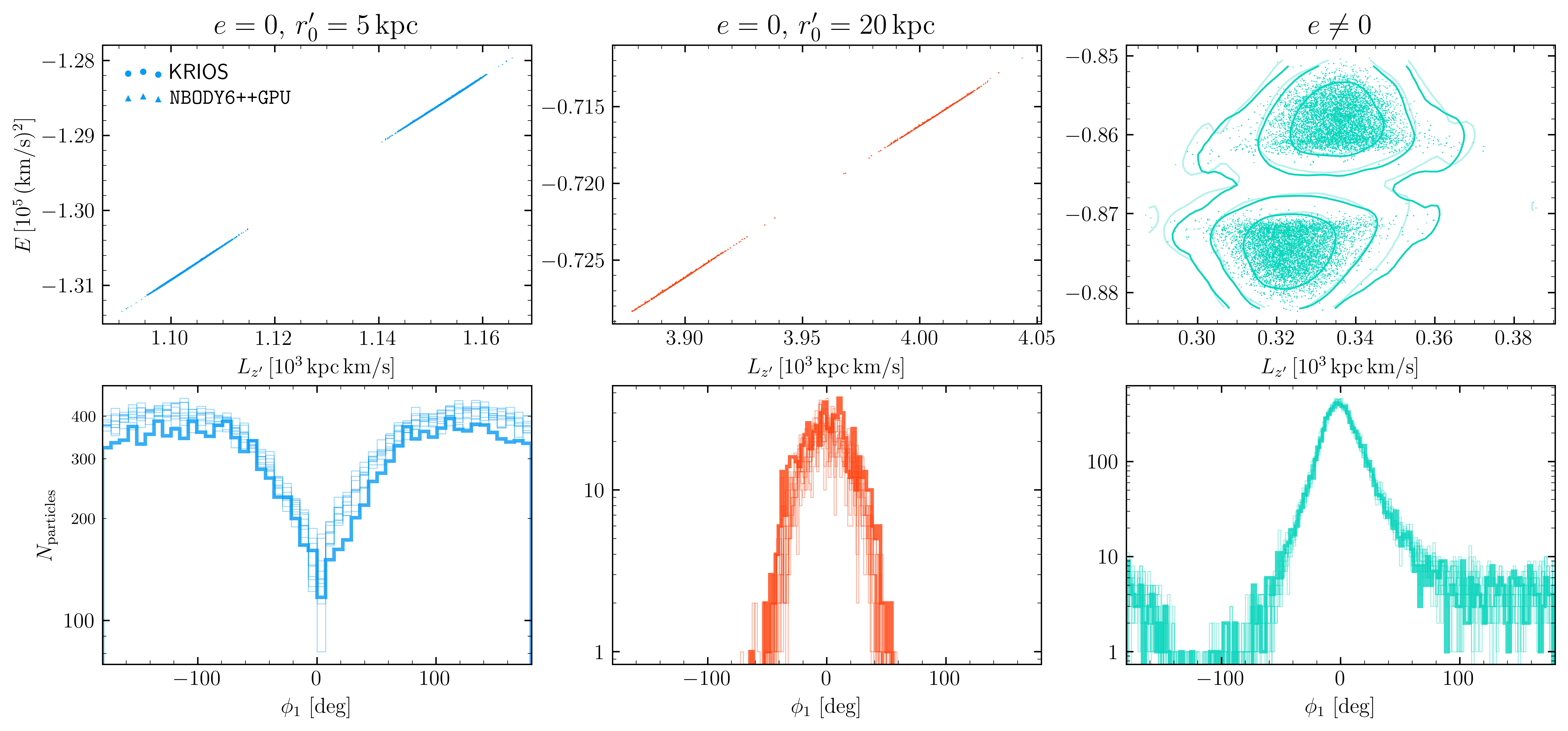
now compare the streams themselves. The first row of Figure 5 shows the distribution of two of the integrals of motion5 of the
particles outside the bound radius of the cluster (defined in Section 2.2). The integrals of motion form a bimodal distribution, with the two peaks corresponding to the leading and trailing tails of the stream.
The leading (trailing) tidal tail emanates from near the \(L_{1}\) (\(L_{2}\)) Lagrange point [51], placing the escapers at lower (higher) \(L_{z'}\) and \(E\). The structure in the integral-of-motion distribution persists even when the stream
traces a complete orbit and the tails are harder to distinguish (e.g. second row, first and third columns, Figure 5). The tidal tails from progenitors on circular orbits follow tracks with \({E\!\propto\!L_{z'}}\) (first and second panels, Figure 5), while the tidal tails from progenitors on eccentric and misaligned orbits present a more complicated picture (third
panel, top row, Figure 5). However, the \(1\sigma\), \(2\sigma\), and \(3\sigma\) contours of the KRIOSand
NBODY6++GPUdistributions are in good agreement here, despite being more diffuse in integrals-of-motion space than their circular-orbit counterparts.
The second row of Figure 5 shows the distribution of particles along the stream track (i.e. in \(\phi_1\)) for KRIOS(darkest line) and each of the NBODY6++GPUruns
(lighter lines). There is a small but consistent offset in the distribution for the circular orbit, which is due to a difference in the mass-loss rate attributable to our \({\gamma\!=\!0.6}\) setting. The eccentric orbit,
which best resembles realistic GC orbits, shows broad agreement at all \(\phi_{1}\).
To more quantitatively compare stream models, we compare the probability distribution functions predicted by KRIOSand NBODY6++GPUfor \({(L_{z'}, E)}\) and \({(\phi_{1},\phi_{2})}\). We use two statistics, the Kullback-Leibler divergence [88], [89] and Earth Mover’s distance [90], to quantify the disagreement between a stream model (“A")
and its NBODY6++GPUcounterpart (”NB"): \[\begin{align}
\tag{10} {\rm KLD}_{A} &= \sum_{x\in X} \rho_{\rm NB}(x) \ln {\rho_{\rm NB}(x) \over \rho_{A}(x)} \\
\tag{11} {\rm EMD}_{A} &= \min_{f\in\mathcal{F}(\rho_{A},\rho_{\rm NB})} \, \sum_{ij} f_{ij} \, d(x_{i}, x_{j}),
\end{align}\] where \(f_{ij}\) is the \({(i,j)}\) element of the flow matrix \(f\) that maps \(\rho_{A}\) onto \(\rho_{\rm NB}\) and \(d(x_{i},x_{j})\) is the distance between those probability distribution
elements. The KLD measures how different an approximate distribution \(\rho_{A}\) is from the ground-truth distribution \(\rho_{\rm NB}\). The EMD, on the other hand, measures the “cost" of
manipulating \(\rho_{A}\) until it agrees with \(\rho_{\rm NB}\). The key difference between these metrics is that the KLD is ignorant to the approximation’s cost6 in a way that is measured directly by the EMD. When estimating \(\rho\), \(f\), and \(d\), we take a random subsample from the more-populated model such that both distributions are estimated from the same number of particles. This allows us to use Monte Carlo approximations to the KLD and EMD in equations 10 and 11 .
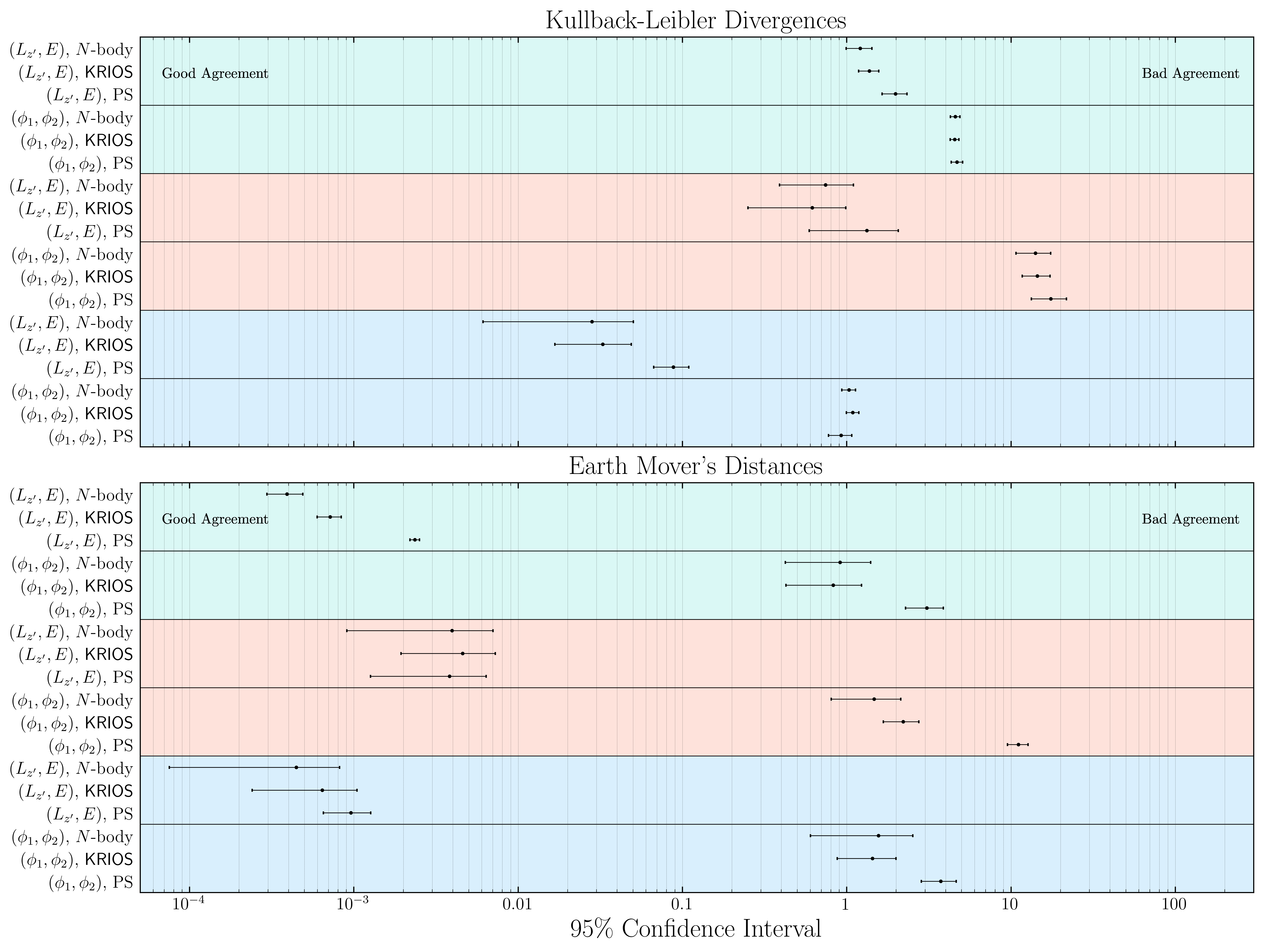
Figure 6 shows the 95% confidence intervals for the KLD and EMD, calculated for each of three comparisons:
Pairs of
NBODY6++GPUruns from the ensemble compared to each other (first row). This number is a proxy for the minimum measurable KLD or EMD for the comparison, as they measure the intrinsic scatter between two different realizations of the same \(N\)-body initial conditions.KRIOScompared to each of the
NBODY6++GPUruns (second row).Particle-spray runs ([91] progenitor, [38] escaper distribution function) compared to
NBODY6++GPUruns (third row).
The comparisons are calculated for each of the three test orbits (shown in different colors), and for the predicted distributions in \((L_{z'},E)\) and \({(\phi_{1},\phi_{2})}\) (sets divided by solid black horizontal lines).
In almost every case, KRIOSreplicates the NBODY6++GPUprediction for the \((L_{z'},E)\) distribution better than particle spray. This is more readily apparent in the EMD scores. In all but two cases—the
KLD measured in \({(\phi_{1},\phi_{2})}\) space for \(r_{0}'\!=\!5\,{\rm kpc}\) and the EMD measured in \((L_{z'},E)\) space for \({r_{0}'\!=\!20\,{\rm kpc}}\)—KRIOShas a better mean score than the corresponding ensemble of particle-spray runs. The improvement is especially large for the predicted distribution of the integrals of motion in the
eccentric orbit case, and for the distribution along the stream track in the case of circular orbits. These results suggests that, overall, KRIOScan reproduce the relevant evolution and stream properties of full NBODY6++GPUruns in a fraction
of the time, with a significantly higher fidelity than equivalent particle-spray runs.
3.2 Statistical and Systematic Variations between KRIOSand Particle-Spray Models↩︎

Having shown that KRIOScan produce streams with similar properties to those expected from NBODY6++GPU we can now explore a wider range of orbits and compare the predictions from KRIOSto those from various particle-spray methods. While it
is possible for sets of particle-spray models to match the properties of NBODY6++GPUor KRIOSstreams on average, it is not clear that they capture the statistical variation inherent in the \(N\)-body problem.
All three stream-modeling methods exhibit inherent stochasticity due to the random sampling of the particles’ initial positions and velocities. But in the case of particle-spray codes, the stochastic “initial” conditions are introduced at the time of
escape, as random draws from a distribution function of escaper properties. This ignores the well-known stochastic variation in the cluster evolution itself, which can produce changes in the cluster’s mass and radii over time.
To that end, we compare predictions for the integral of motion distribution made by KRIOSand particle-spray ensembles over the wider range of orbits drawn to span the space of known GC orbits (Section 2.3; Figure
3). Figure 7 shows the statistical variation between independent KRIOS(triangles) and particle-spray (circles) runs, as well as the systematic differences when these models
are compared to each other (dashes). The models are compared at apogalacticon and in integrals-of-motion space using the EMD, which we found to be the more sensitive of the two metrics used in Section 3.3. Based on
the results of those tests, we take the KRIOSprediction to be closer to the NBODY6++GPUrun. Large differences between particle-spray and KRIOSthus highlight which orbits require a more accurate treatment of the escape physics than is
achievable with particle-spray methods.
The EMD between two particle-spray models with different seeds (circle markers) is consistently lower than for KRIOS. This matches our expectation, as changing the random number generator’s seed simply changes the starting point when drawing from a particle-spray model’s constant distribution function, while in the KRIOSapproach there is additional stochastic variation from the internal cluster dynamics. This suggests that ensembles of particle-spray models may underestimate stream-to-stream variability. On the other hand, an ensemble of KRIOSmodels is likely needed to confirm that an interesting feature of any particular stream is not an artifact of stochastic variation due to the cluster initial conditions or dynamical evolution. In future applications of KRIOS where a stream model is consistent with a dark matter subhalo flyby, for example, such considerations are critical.
As in Figure 6, the EMD between KRIOSand particle-spray models (lines with errorbars) shown in Figure 7 should be compared against the statistical variations between KRIOSruns to gauge the difference between the predictions. If the ratio between the two is high, then particle-spray models systematically deviate from KRIOSin a way that calls into question whether particle spray is accurate for these orbits.
![Figure 8: A comparison between the known MW stellar streams [5] and simulated orbits (labeled in the right column) in apogalacticon/perigalacticon space (top row) and integrals-of-motion space (bottom row). Each orbit is color coded by the ratio {\langle{\rm EMD}_{{\sf K},{\rm PS}}\rangle/{\rm EMD}_{\sf{K},\sf{K}}}, which controls for statistical variations expected from KRIOSruns with the same initial conditions. Particle spray models show poorer agreement to KRIOSwhen the progenitor is subject to strong tidal fields or is tightly bound to the host.](/article/2602.13385/normalized_emd_comps.png "fig:")
3.3 Analysis of Systematic Differences between KRIOSand Particle Spray for Realistic Orbits↩︎
We now compare the streams generated by KRIOSto those generated be particle spray across the 10 Figure 3 orbits in the MWPotential2022 potential. In Figure 8, we show the ratio of the EMD KRIOSstreams vs. particle-spray to the EMD between two different KRIOSruns in both \({(\phi_{1},\phi_{2})}\) (top row) and \({(L_{z'},E)}\) (bottom row) space. This ratio allows us to focus on the systematic agreement between the streams by normalizing to the statistical variation expected between cluster models with different realizations of the
same initial conditions. We show these values calculated near their last perigalacticon passage (top row) and apogalacticon (bottom row). Overall, these results suggest that the added computational expense of creating stream models with a full \(N\)-body calculation is necessary when the stream is subject to strong tidal forces (i.e., small perigalacticon) or when it is tightly bound to the host galaxy (low \(E\)), especially if it is
near the effective-potential barrier (high \(|L_{z'}|\)). Any inferences made about the properties of mock stellar streams made using particle-spray models [92] should be applied with caution to streams that have these properties. The stellar stream associated with the M92 globular cluster [93], for example, is susceptible both to modeling errors on the sky plane and in the integrals of motion. Streams like the Fjörm [94] system are less susceptible to integrals-of-motion errors, but, at apogalacticon, sky-plane variations will be pronounced. The Gunnthrá stream [95], which may be debris from \({\omega\,\,{\rm Cen}}\) [96],
appears to lie beyond the effective-potential barrier and is tightly bound to the Milky Way [97]; disagreement in stream integrals-of-motion is high in
this region.
On the other hand, several scientifically interesting streams can be robustly modeled with particle-spray according to these metrics. The GD-1 stream [22], not shown in Figure 8, is currently near perigalacticon [44] and
has one of the largest \(|L_{z'}|\) values of all known stellar streams [98]. The Kshir stream, which has
properties similar to GD-1 [99], is shown in the bottom row of figures at high \(|L_{z'}|\), similar to Orbit 9.
Particle-spray models of streams on orbits of this kind will largely be consistent with KRIOS(and hence with NBODY6++GPU).
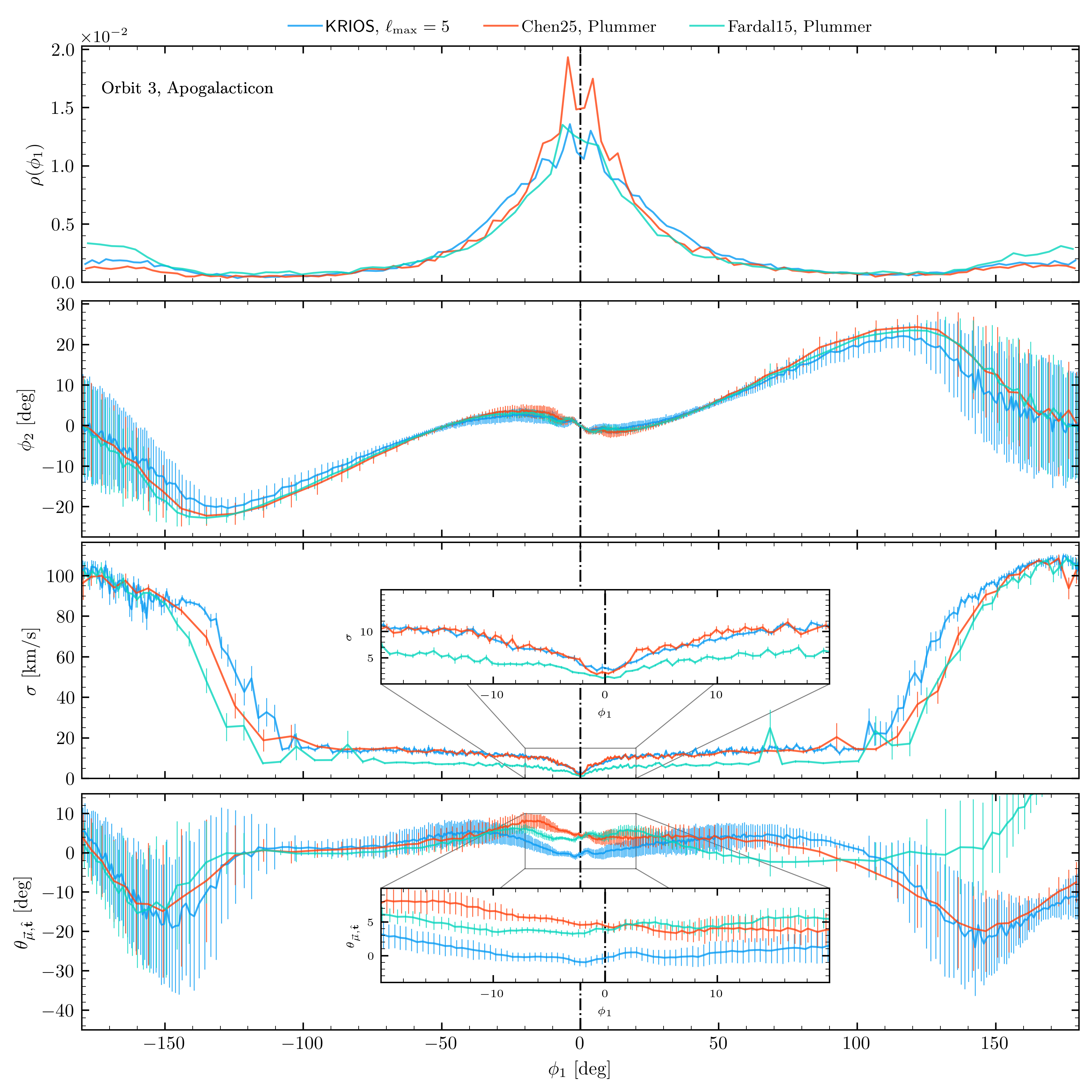
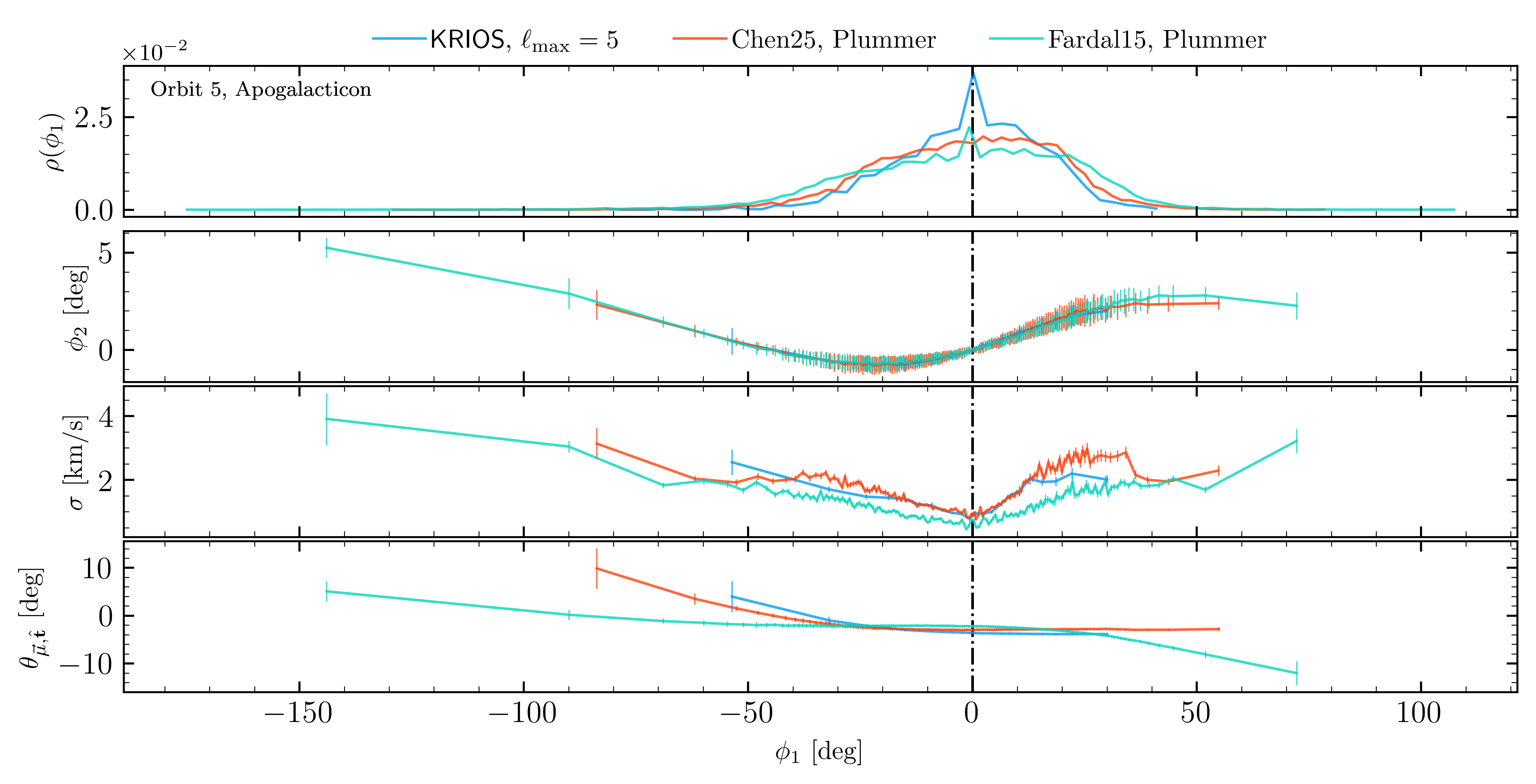
Interactions of streams with Galactic substructure, whether dark or baryonic, is thought to perturb the stream density \(\rho(\phi_{1})\) and velocity dispersion \(\sigma(\phi_{1})\) profiles along the stream track. It is critical that we understand which features of these profiles originate from the model assumptions, so that they are not mistaken for external perturbations. This is especially important given that several different escape prescriptions are commonly used in particle-spray models, yet there are very few tests of which prescriptions best reproduce \(\rho(\phi_{1})\) and \(\sigma(\phi_{1})\) for globular cluster streams. To examine differences in the predicted profile, we select particles that are unbound from the cluster and bin them in \(\phi_{1}\) from the inside out, starting at the progenitor, such that the number of particles in each bin \(N_{\rm particles\,in\,bin}\!\geq\!100\) and the bin width \({\Delta\phi_{1,{\rm bin}}\!\geq\!0.5\,{\rm deg}}\). This binning strategy is chosen to accentuate differences in the \(\rho(\phi_{1})\) and \(\sigma(\phi_{1})\) profiles. Each distribution is computed from all particles in the stream (as opposed to Section 3.1, where the distributions were downsampled in order to calculate the KLD and EMD). We take many draws from each bin’s particles, detrend their velocities by subtracting a linear term \(\bar{v}(\phi_1)\) within the bin, and then estimate the local 1D velocity dispersion \({\sigma\!=\!\sqrt{\mathop{\mathrm{tr}}(\boldsymbol{\Sigma})/3}}\), where \(\boldsymbol{\Sigma}\) is the covariance matrix of the detrended velocities. By the central-limit theorem, this nonparametric bootstrapping method [100] reduces the uncertainty in \(\sigma(\phi_{1})\) as we take more samples. We also calculate the average misalignment angle between the particles’ proper motions and unit vector tangent to the stream track, i.e. \({\cos\theta_{\boldsymbol{\mu},\hat{\boldsymbol{t}}}(\phi_{1}) \!\equiv\!{1\over N}\sum_{i=1}^{N}(\hat{\boldsymbol{\mu}_{i}}\cdot\hat{\boldsymbol{t}}(\phi_{1,i})})\), which can also be used to probe the stream kinematics [36]. We parameterize \(\phi_{2}(\phi_{1})\) with a smoothed B-spline in order to calculate the tangent vector \(\hat{\boldsymbol{t}}(\phi)\) and hence the misalignment angle \(\theta_{\boldsymbol{\mu},\hat{\boldsymbol{t}}}(\phi_{1})\).
As examples of stream structure that varies with the underlying modeling technique, we show the KRIOSand particle-spray models for Orbit 3 (Figure 9) and Orbit 5 (Figure 10). KRIOSand particle spray disagree on these orbits, more so for Orbit 3 than Orbit 5 (see Figures 7, 8). The latitude vs. longitude trends agree, which suggests that KRIOSand particle spray are equally capable of integrating particles forward in the same host potential. Variations in \(\rho(\phi_{1})\) are most notable near the progenitor, where different particle-spray distribution functions better replicate the density fluctuations predicted by KRIOSon different orbits. There is a notable demarcation between \(\theta_{\boldsymbol{\mu}, \boldsymbol{t}}(\phi_{1})\) predictions near the progenitor for the Orbit 3 stream. The velocity dispersion profiles disagree as well, but this effect is seen most strongly in the tidal tails. The Orbit 3 stream, for example, systematically underestimates \(\sigma(\phi_{1})\). Both particle-spray models for the Orbit 5 stream are more spread out in \(\phi_{1}\) than the KRIOSmodel, which may be the source of the disagreement in \(\sigma(\phi_{1})\) and \(\theta_{\boldsymbol{\mu},\hat{\boldsymbol{t}}}(\phi_{1})\). These results illustrate that subtle differences between models are imprinted on the predicted kinematics of the stream.
4 Discussion↩︎
We showed in Section 3.3 that the predicted stream is sensitive to the implementation details of the underlying modeling technique. Particle-spray codes that sample escapers from some distribution function, for
example, might ignore changes to the progenitor induced by the host potential or that mass loss is correlated with the strength of the tidal field. Additionally, stream-modeling techniques often assume the progenitor is spherically symmetric (e.g.,
CMC’s implementation of the Hénon method), which substantially affect the mass-loss rate—and hence also the predicted stream. This is particularly important in light of several recent works that examine streams from GCs simulated with
CMC, ranging in complexity from GCs on circular orbits in a static and spherical MW [27], [52] to GCs on non-periodic orbits in an evolving and clumpy MW-like FIRE cosmological simulation [56]—see also [101], [102]. Here, we leverage KRIOSto explore potential discrepancies between comparable stream-modeling techniques more concretely. We focus primarily on Orbit 3, as Figure 7 shows that
this orbit shows the least stochastic scatter between similar KRIOSand particle-spray models, while showing significant disagreement between KRIOSand particle spray (as also seen in Figure 8).
4.1 A spherically symmetric progenitor is usually sufficient to model escaping stars↩︎
Though CMCsimulations feature collisional dynamics and a particle-based GC potential, creation of model streams requires modeling the trajectories of escaping stars in post-processing since the full potential of the host galaxy is
represented only by the tidal tensor. Bodies are removed from CMCupon achieving an orbital energy or apocenter sufficient for escape (often in the GC’s core), and then integrated in the mutual potential of the GC and its host galaxy. The GC
potential is made analytic by fitting a Plummer sphere [56]—or a three-component Plummer sphere to better reproduce the cores of
evolved GCs [27], [52]—to the raw CMCpotential and
interpolating the fitting parameters coarsely in time (a few snapshots per half-mass relaxation time). The trajectories of stars forming a stream from a CMCcluster model thus only experience a fairly rough approximation of the true potential
at the boundary between the GC and host galaxy. By comparison, particle-spray models often assume a fixed Plummer progenitor, i.e. constant mass and half-mass radius. The self-consistent potential maintained by KRIOS, on the other hand (Equation 1 ), is tuned to the GC’s true configuration more accurately and at higher temporal resolution. Additionally, escapers are subject to the same SCF even after they leave the cluster. The model used in KRIOSis therefore
more self-consistent and well-resolved on the relevant timescales within the cluster, and should be preferable to the CMCapproach. We can use the structure of the SCF to test the effect of the assumption of a spherically symmetric cluster on
the accelerations felt by escaping stars directly, since setting \(\ell_{\mathrm{max}}=0\) is equivalent to forcing the cluster potential to be spherically symmetric as it is in CMCand many particle spray
code.
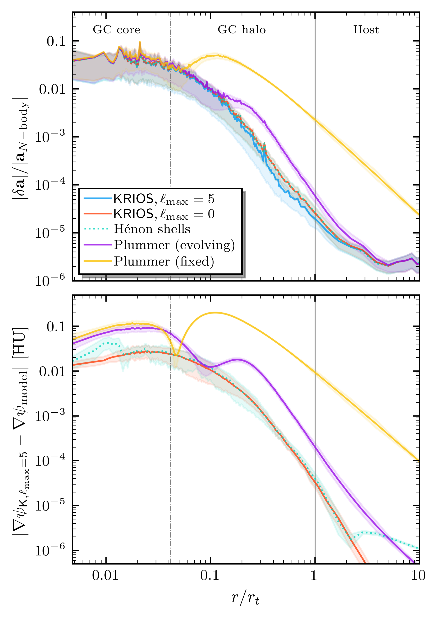
We can probe the effectiveness of each progenitor model by comparing the accelerations from each model to those calculated by direct \(N\)-body summation. The top panel of Figure 11 shows the acceleration residuals [103], [104]
for different mean-field progenitor models, compared to the true values \(N\)-body accelerations.The Plummer progenitor that does not take cluster evolution into account (yellow curve), which is often used in particle-spray
methods, poorly captures the particle accelerations. We see significant improvement if we use the instantaneous cluster mass and scale length for the Plummer potential [56]. A multi-component Plummer potential fit would result in further improvement [52], and using
CMC’s exact spherical-shell potential \({\psi_{\rm cluster}\!=\!-{GM_{\rm enc}(<r)\over r}}\) (dotted green curve) is better still, agreeing well with the spherically symmetric KRIOSSCF (red curve). The
fiducial KRIOSprofile (\({\ell_{\rm max}\!=\!5}\); blue curve) best reproduces the target accelerations. By construction, it is able to resolve tangential acceleration components in a way that spherically symmetric fields
cannot. The bottom panel of Figure 11 shows how the accelerations, expressed as the gradient of the potential in Hénon units, compare to the fiducial model. Here, we see the Plummer-sphere approximations (both fixed
and evolving) separate from the non-Plummer-sphere approximations in the GC’s core, as well as how the zeroth-order mode of the SCF disagrees with the spherical-shell potential for \({r\!\lesssim\!0.5\,r_{\rm core}}\).
![Figure 12: The fiducial KRIOSmodel for the Orbit 3 stream compared to three models near the last apogalacticon passage: one with an SCF progenitor [59], one with a Plummer progenitor, and one with no progenitor. There does not appear to be immediate improvement in the modeling with improved treatment of the progenitor, assuming that the progenitor is fixed.](/article/2602.13385/stream_comp_Orbit_3_is_apo_True_chen_feb5.png "fig:")
Figure 12 shows the impact of different progenitor prescriptions on the stream, which again are slight disagreements in \(\rho(\phi_{1})\) and \(\sigma(\phi_{1})\). There is no clear connection between improving the treatment of the progenitor potential—from no progenitor at all, to a Plummer model, to an SCF model—and the accuracy of stream density, morphology, or kinematics. Interestingly, it is the intermediate model (Plummer) that has the worst velocity dispersion agreement with KRIOSin the tails, but best replicates the density variations near the progenitor. The implication here is that there is an upper limit on the degree to which particle spray can be improved with more accurate initializations of a fixed progenitor. However, related improvements to modeling the progenitor’s internal dynamics, such as explicit treatment of strong encounters (in the process of being added to KRIOS), still can substantially affect stream properties [27], [105].
4.2 Spherically (a)symmetric KRIOS progenitors produce statistically similar streams↩︎
The \({\psi_{\rm eff}(\mathbf{r})\!=\!E_{J}}\) surface through which a bound particle with Jacobi integral \({E_{J}\!=\!{v^{2}\over 2} + \psi_{\rm eff}}\) cannot pass is not spherically symmetric. Particles escape primarily in the vicinity of the \(L_{1}\)/\(L_{2}\) Lagrange points, especially those whose Jacobi integral is only marginally above the escape threshold [51], [52]. Figure 2 of , which shows the normal distribution of escapers’ spherical phase-space coordinates from \(N\)-body runs, provides further evidence of escape anisotropy.
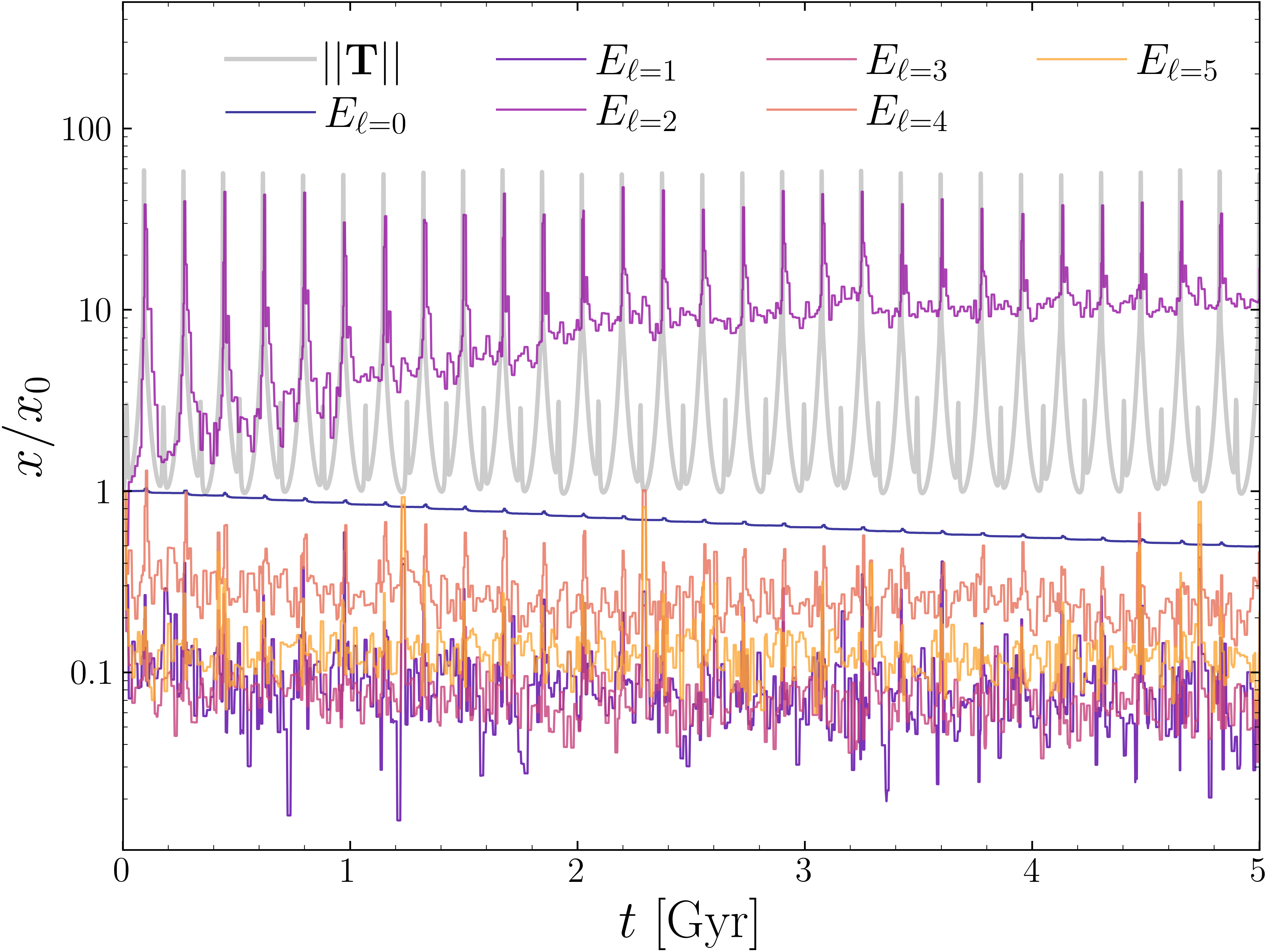
The asphericity of the GC’s mass distribution can be measured by the power in each of the \(\ell\) modes, computed as \({E_{\ell} \!=\! \sum_{nm} |a_{n \ell m}|^{2}}\) , where \(\{a_{n\ell m}\}\) are the SCF’s basis coefficients. The GC is spherically symmetric if \({E_{\ell}\!=\!0}\) for all \({\ell\!>\!0}\). Figure 13 compares the eccentric validation model’s SCF \(\ell\)-mode power spectrum and the tidal tensor’s Frobenius norm \(||\boldsymbol{T}||\), all normalized by their initial values, as a function of time. This time-series data demonstrates how KRIOSclusters evolve when coupled to external tidal fields. The \({\ell\!=\!0}\) monopole term loses power as the cluster loses mass. The \({\ell\!=\!1}\) dipole term measures how well the SCF is centered on the cluster.7 The asphericity of the system is represented by the \({\ell\!\geq\!2}\) modes [59], [106], [107]. A significant amount of power is deposited in the \({\ell\!=\!2}\) quadrupole term, which is an instantaneous measure of the cluster’s oblateness [108], during each tidal shock (either at perigalacticon or during a disk passage). Aspherical distortions of this kind are qualitatively consistent with MWGC observations [109].
Despite this measurable change in the cluster’s oblateness, the integrals-of-motion and sky-plane EMD scores between the fiducial \({\ell_{\rm max}\!=\!5}\) models and the models where spherical symmetry is enforced
(\({\ell_{\rm max}=0}\)) have the following ranges when evaluated at apogalacticon: \[\begin{align}
{\langle {\rm EMD}_{{\sf K}5, {\sf K}0} \rangle \over {\rm EMD}_{{\sf K}5, {\sf K}5}} \in \begin{cases} (0.5, 1.4) &(L_{z'},E), \\ (0.7, 1.9) &(\phi_{1},\phi_{2}). \\
\end{cases}
\end{align}\] This suggests that stream models produced by Hénon-based \(N\)-body codes like CMCwill only suffer from mild disagreement due to the assumed spherical symmetry of the progenitor, as long as
the progenitor is properly incorporated when calculating escaper dynamics (Section 4.1). We have not made direct comparisons between CMCand KRIOSmodels, so the degree to which their predictions
for stream substructure (e.g., gaps, spurs) agree warrants investigation in future studies.
4.3 Mass-loss Rate Variability in Stream Modeling↩︎
Our particle-spray models, to this point, have assumed a constant mass-loss rate (i.e., escapers drawn from the distribution functions at each timestep). Here, we consider the impact of a variable mass-loss rate. The third panel of Figure 2 in [56] shows that the number of ejected particles peaks sharply during perigalacticon passages, which is corroborated by KRIOS(see the green
curve in the second panel of Figure 4). Variable mass-loss rates can be added to particle-spray models by passing an array of particle counts to be released during each timestep to the relevant gala
stream-generation method8 or through post-processing of the stream data itself [110]. Candidate variable mass-loss rates include \({\dot{M}(t)\!\propto\! M(t)^{a}\Omega(t)^{b}r_{\rm hm}(t)^{c}}\) [72], where \(\Omega(t)\) increases during perigalacticon passages, and , which uses an analytic prescription for the mass-loss rate as a function of the orbit’s radial phase to build its
distribution function. The latter is more applicable to particle-spray methods that do not track the progenitor mass or half-mass radius. Neither prescription accounts for disk shocks that heat up the progenitor, and by default gala assumes a
constant mass-loss rate.
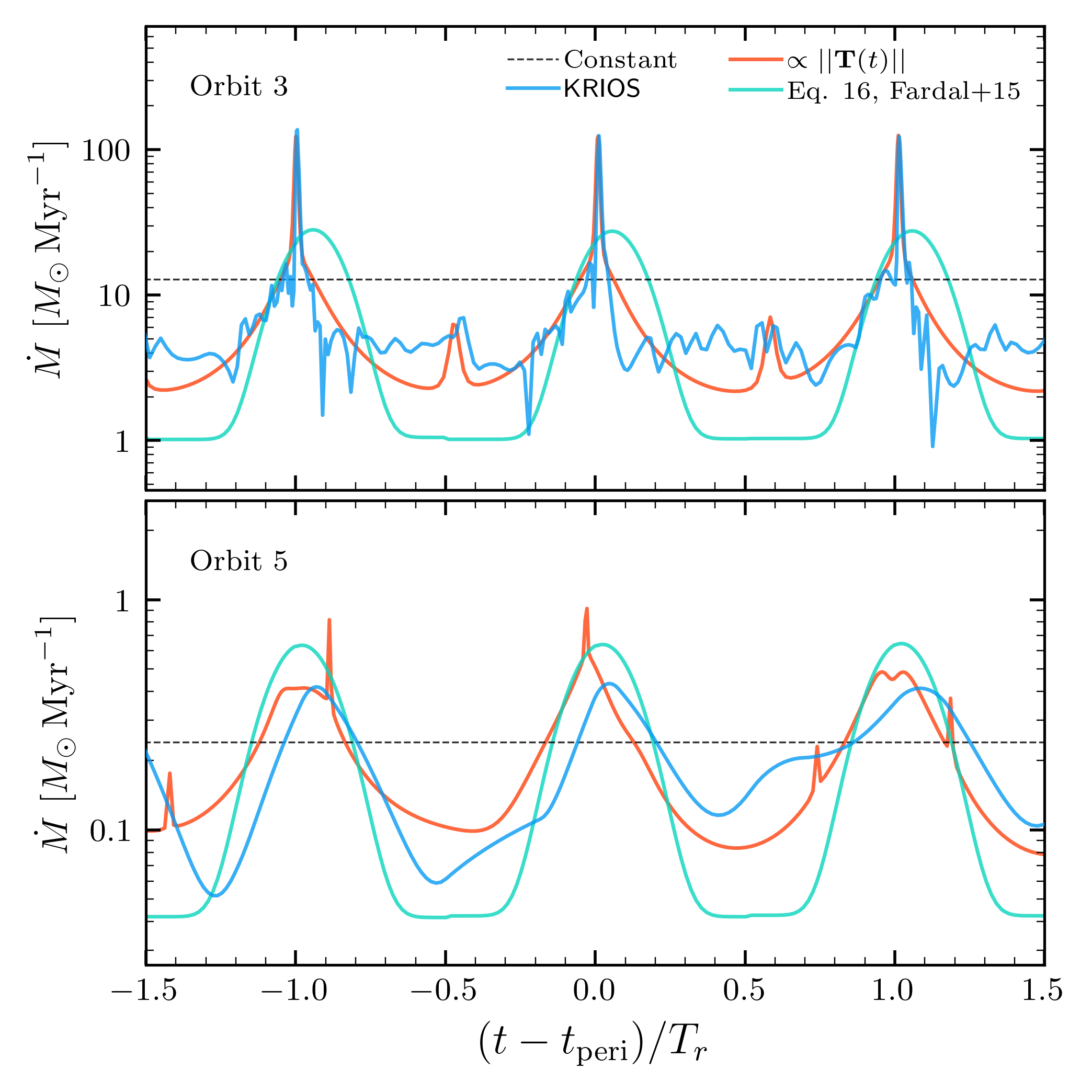
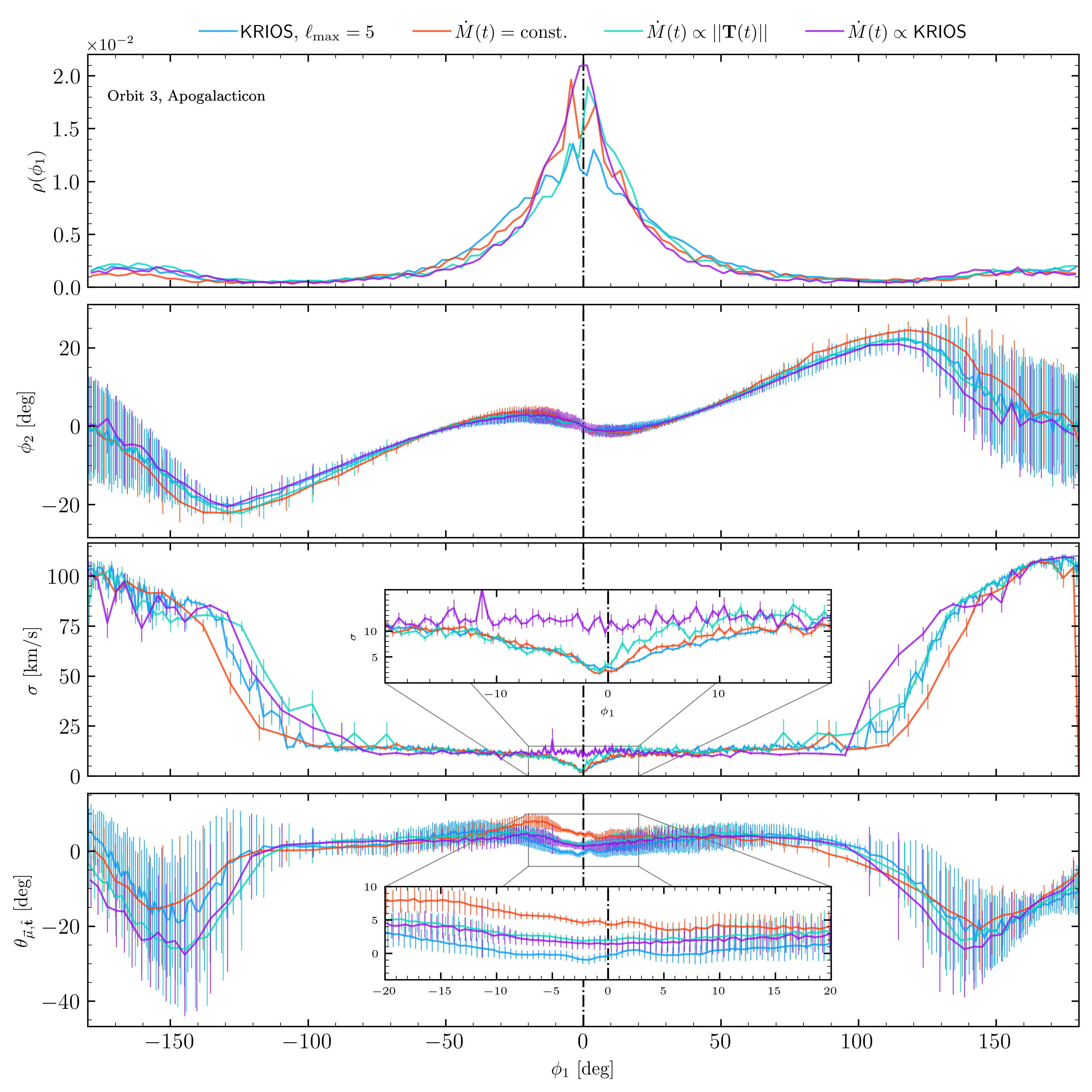
Figure 14 shows the mass-loss rate in the Orbit 3 and Orbit 5 KRIOSsimulations (blue) for three complete orbits and compares them to the following mass-loss prescriptions: constant (black dashed line), Equation 16 of (green), mass loss directly proportional to the tidal tensor’s Frobenius norm (red), and mass loss proportional to the mass-loss history from the KRIOS data (purple). A constant mass-loss rate is clearly a poor fit to the Orbit 3 data, as the peak mass-loss rate at perigalacticon (which coincides with a disk passage, see Figure 3) is \({\sim10\times}\) the average. Additionally, the mass-loss rate is suppressed after these peaks; this is likely attributable to the unavailability of easily stripped particles that are replenished through continued relaxation when the cluster is subject to comparatively weak tidal forces. For the Orbit 5 model, there are only \(\lesssim\!5\) particles ejected per integration timestep, so a constant mass-loss rate heuristic is likely acceptable in this context. The tidal tensor captures disk shocks (see the peaks in the red curve), which might make it suitable as a generalized mass-loss rate prescription.
Figure 15 shows how these mass-loss rates manifest in models of the Orbit 3 stream. The blue curve shows the fiducial KRIOS\({\ell_{\rm max}\!=\!5}\) model that is also shown in Figures 9 and 12. The green curve shows the particle-spray model with distribution function and Plummer progenitor (see Figure 12) where the mass-loss rate is constant, and the red curve shows the same particle-spray model where the mass-loss rate is set by passing the \(||\boldsymbol{T}(t)||\) time-series data to the stream-generation method. The purple curve’s disagreement with the KRIOS model is likely due to all of the other modeling differences (e.g., static Plummer sphere progenitor and escaper distribution function). Further investigation is needed into variable mass-loss rate prescriptions that better replicate the numerical experiments we have carried out with KRIOSin this study, e.g. ones that take the recent history of the tidal tensor along the orbit into account.
5 Conclusions↩︎
In this paper, we expand the scope of the KRIOShybrid \(N\)-body code that was recently introduced in by modeling tidal debris from globular clusters orbiting a host galaxy. Realistic MW potential models are used to
validate KRIOSagainst known, successful stream-modeling techniques. There is good agreement between KRIOSand NBODY6++GPUwhen the respective codes model the internal evolution of GCs in an external tidal field, as well as their resultant
debris. It is found that, on an orbit consistent with realistic MWGC orbits, KRIOSreplicates the sky-plane and integrals-of-motions distributions from comparable NBODY6++GPUruns.
5.1 Conclusions for Stream Modelers↩︎
We use a collection of MilkyWayPotential2022 sample orbits, spanning the region of orbit space occupied by known MW streams, to test how KRIOSand particle-spray models might disagree in scenarios similar to those found in the observational
data. Particle-spray results deviate from KRIOSin the following scenarios:
The GC is subject to strong tidal forces during its orbit, characterized by small perigalacticon and apogalacticon distances. The Fjörm and M92 streams are examples of such systems. Differences in the stream’s distribution on the sky plane are most apparent when they are near apogalacticon.
The GC is tightly bound to the host galaxy. This applies to circular (M92, Gunnthrá) and radial (Fjörm) orbits alike. Systems of this kind lead to disagreements in how well the integrals of motion of the stream stars are conserved.
The most common form of disagreement between KRIOSand particle-spray stream models are in the resolution of density fluctuations near the progenitor and the velocity dispersion of the tails far from the progenitor. Inferences made about the morphology of the GC’s extratidal features or the kinematics of sparsely populated regions in the GC streams should consider whether the progenitor physics are appropriately taken into account. Even when particle spray reproduces the stream (as measured statistically by the KLD or EMD), its internal structure depends on the particle-spray implementation (Section 3.3; Figures 9 and 10). Several different escaper distribution functions and mass-loss prescriptions should be considered in order to eliminate these as explanations for substructure. The mass-loss rate is computed self-consistently with KRIOS, so no prescription is needed. We find that there are limitations to more sophisticated models of a fixed progenitor in particle-spray methods; rather, it is likely more important to incorporate time-dependent progenitors that accommodate variable mass-loss rates, and to consider the impacts of a realistic stellar mass function and ejection via strong encounters [27], [105], [111].
Assuming a spherical model of the progenitor cluster, as is done in CMC, is sufficient, in most cases, to model the escape of stars from the cluster (Section 4.1) and resolve the internal
cluster dynamics (Section 4.2) when predicting the density, velocity dispersion, and misalignment along the stream. This may not be the case for all clusters, e.g. if there is internal rotation [109], [112]. In the future, we plan to implement time-dependent host potentials from cosmological
simulations, as there are known defects with stream models in a smooth [113] or static [114] host potential. This will be the foundation for future cosmological stellar stream catalogs [56], [92], where the progenitor’s \(N\)-body code is designed specifically for this use case.
KRIOSruns are terminated once there are only 100 particles in the core (i.e., core collapse, see Section 2). \({N\!\leq\! 4}\) microphysics [84] are not yet accounted for, e.g. the production of binary star systems [115], which are critical to modeling the post-collapse evolution of globular clusters. Figure 2 of [116]
demonstrates that these phenomena have a tangible impact on stream production as well, which necessitates their inclusion in future implementations of KRIOS. In future work, we plan to include both three-body binary formation and strong encounters between
single and binary stars. We will also model stellar/binary evolution with a realistic initial mass function [117], [118] using the COSMIC population-synthesis code [78].
Acknowledgments↩︎
We thank Dany Atallah for helpful discussions that improved the quality of the manuscript. This work was supported by the National Science Foundation under Grants Numbers AST-2510181 to the University of North Carolina, AST-2510183 to Northwestern University, and by NASA ATP Grant 80NSSC24K0687. CR also acknowledges support from an Alfred P. Sloan Research Fellowship and a David and Lucile Packard Foundation Fellowship. BTC was partially funded by the North Carolina Space Grant’s Graduate Research Fellowship. TS gratefully acknowledge the support of the NSF-Simons AI-Institute for the Sky (SkAI) via grants NSF AST-2421845 and Simons Foundation MPS-AI-00010513. TS was also supported by NASA through grant 22-ROMAN22-0013. This work was supported by a research grant (VIL53081) from VILLUM FONDEN. CR, KT, and RS also thank the organizers of the workshop “Interconnections between the Physics of Plasmas and Self-gravitating Systems”, supported by NSF Grant PHY-2309135 to the Kavli Institute for Theoretical Physics (KITP). This work was also co-funded by the European Union (ERC, BeyondSTREAMS, 101115754) grant. Views and opinions expressed are however those of the author(s) only and do not necessarily reflect those of the European Union or the European Research Council. Neither the European Union nor the granting authority can be held responsible for them.
We would like to thank the University of North Carolina at Chapel Hill and the Research Computing group for providing computational resources and support that have contributed to these research results. We thank Stéphane Rouberol for the smooth running
of the Infinity cluster of the Institute of Astrophysics of Paris, where the NBODY6++GPUruns were performed.
KRIOSsimulations, and their subsequent analyses, depend on the following software packages: GNU Compiler Collection9, GNU Scientific Library [119], OpenMP [120], numba [121], NumPy [122], SciPy [123], pandas [124], Matplotlib [125], Astropy [126], gala [76], galpy [82], Python Optimal Transport [127].
Data Distribution↩︎
There is a public GitHub repository (https://github.com/BrianTCook/krios_ii_paper_supplement) containing a subset of the data presented in this paper, as well as a Jupyter notebook that produces relevant observables from that data. Additional data will be made available upon request to the authors.
To facilitate the reproducibility of our NBODY6++GPUresults and allow its use of the MWPotential2014 external field, we created a fork of the original NBODY6++GPUrepository containing these corrections (https://github.com/KerwannTEP/Nbody6ppGPU). Additionally, we provide pre- and post-processing scripts at https://github.com/KerwannTEP/NB6-MW2014-Tools.
6 MW Potential Models in KRIOS↩︎
6.1 Spherical Components: Galactic Bulge, Hernquist Potential, and NFW Halo↩︎
The density of the MWPotential2014 Galactic bulge is defined in the following way10: \[\begin{align}
\rho(r') &= \rho_{0} \left({r_{c}\over r'}\right)^{\alpha}\exp\left[-(r'/r_{c})^{2}\right],
\end{align}\] where we set the reference radius equal to the cutoff radius for convenience. The enclosed mass, as a function of \(r'\), is \[\begin{align}
M_{\rm enc}^{\rm Bulge}(r') &= 4\pi \int_{0}^{r'} {\rm d}r'' \, r''^{\,2} \rho(r'')\notag \\
&= 4\pi \rho_{0} r_{c}^{3} \int_{0}^{r'/r_{c}} {\rm d}u \, u^{-\alpha+2}\exp(-u^{2}).
\end{align}\] The choice of reference radius, along with the bulge mass, dictates \({\rho_{0} \!=\! M_{b}/\left(4\pi r_{c}^{3}\int_{0}^{\infty}\! {\rm d}u \, u^{-\alpha+2}\exp[-u^{2}]\right)}\). This means we can
write the enclosed mass as a function of \(M_{b}\): \[\begin{align}
M_{\rm enc}^{\rm Bulge}(r') &= M_{b} {\int_{0}^{r'/r_{c}} {\rm d}u \, u^{-\alpha+2}\exp(-u^{2}) \over \int_{0}^{\infty} {\rm d}u \, u^{-\alpha+2}\exp(-u^{2})} \notag\\
&= M_{b}{\gamma(s, x)\over \Gamma(s)},
\end{align}\] where \({x\!=\!(r'/r_c)^2}\), \({s\!=\!{1\over 2}(3-\alpha)}\) and \(\gamma(a,x)\) is the lower incomplete gamma function defined as
\[\begin{align} \gamma(a,x) &= \int_0^x {\rm d}t \, t^{a-1} e^{-t}.
\end{align}\] We use the associated potential implemented in galpyand NBODY6++GPU, which reads \[\begin{align} \label{eq:psi95bulge} \psi_{\rm
Bulge}(r') &= \frac{G M_b}{\Gamma(s)}\bigg(\frac{\gamma(1-\alpha/2,x)}{r_c}-\frac{\gamma(s,x)}{r'}\bigg).
\end{align}\tag{12}\] The bulge potential tends to a non-zero value at spatial infinity: \[\begin{align} \psi_{{\rm bulge},\infty} = {GM_{b} \over r_{c}} \left({\Gamma(1-\alpha/2) \over \Gamma(s)}\right)>0.
\end{align}\] Therefore, if a component of this kind is included in a Galactic model (as it is in MWPotential2014), there will be bound orbits with positive energies up to \(\psi_{{\rm
bulge},\infty}\).
The bulge is spherically symmetric, so only \(f_{v_{r'}}^{\rm Bulge}\) is non-zero and can be computed directly from the enclosed mass: \[\begin{align} f_{v_{r'}}^{\rm Bulge} &= -{GM_{\rm enc}^{\rm Bulge}(r') \over r'^{2}} = -{GM_{b}\over r'^{2}}{\gamma(s,x) \over \Gamma(s)}. \end{align}\] The associated tidal tensor only has one non-zero term in the spherical coordinates of the host frame: \[\begin{align} \partial_{r'}f_{v_{r'}}^{\rm Bulge} &= {2GM_{b}\over r'^{3}}{\gamma(s,x) - x^{s}\exp(-x) \over \Gamma(s)}. \end{align}\] The gravitational potential and enclosed mass for a Hernquist model [128], [129] of total mass \(M_{\rm H}\) and scale radius \(a\) are \[\begin{align} \psi_{\rm H}(r') &= - {GM_{\rm H} \over a} \, {1 \over (1+r'/a)}, \\ M_{\rm enc, \, H}(r') &= M_{\rm H} \, {(r'/a)^{2} \over \left(1+ r'/a\right)^{2}}, \end{align}\] The spherically symmetric potential only has a non-zero gradient in the radial direction, i.e. \[\begin{align} f_{v_{r'}}^{\rm H} &= -{GM_{\rm enc, \, H}(r') \over r'^{2}}. \end{align}\] For this spherically symmetric potential, we only need to compute \(\partial_{r'}f_{v_{r'}}^{\rm NFW}\) to get the tidal tensor: \[\begin{align} \partial_{r'}f_{v_{r'}}^{\rm H} &= {2GM_{\rm H} \over r'^{3}} {(r'/a)^{3}\over (1+r'/a)^{3}}. \end{align}\] The NFW potential [76], [129], [130] can be written in terms of a scale mass \(M_{\rm NFW}\) and scale radius \(r_{s}\) in the following way: \[\begin{align} \psi_{\rm NFW}(r') &= -{GM_{\rm NFW} \over r'} \, \ln\left(1+{r'\over r_{s}}\right). \end{align}\] The enclosed mass, which does not converge for NFW halos, is \[\begin{align} M_{\rm enc, \, NFW}(r') &= M_{\rm NFW} \, g(r'/r_{s}), \end{align}\] where \(g(x) \!\equiv\! \ln(1+x) \!-\! x/(1+x)\). The associated non-zero force and tidal tensor terms (in the spherical coordinates of the host frame) are \[\begin{align} f_{v_{r'}}^{\rm NFW} &= -{GM_{\rm enc, \, NFW}(r') \over r'^{2}}, \\ \partial_{r'}f_{v_{r'}}^{\rm NFW} &= {2GM_{\rm enc}^{\rm NFW}(r') \over r'^{3}}\left(1-{1\over 2 g(r'/r_{s})}\left({r'/r_{s} \over 1 + r'/r_{s}}\right)^{2}\right). \end{align}\]
6.2 Cylindrical Components: Miyamoto-Nagai Disk↩︎
The Miyamoto-Nagai disk potential [129], [131] can be written in terms of the mass
\(M_{\rm MN}\), scale length \(a\), and scale height \(b\): \[\begin{align}
\psi_{\rm MN}(\varrho', z') &= -{GM_{\rm MN} \over \sqrt{\varrho'^{2}+z^{\prime 2}_{ab}}},
\end{align}\] where \((\varrho', \varphi', z')\) are the cylindrical coordinates with respect to the host and \({z'_{ab}\!\equiv\!\sqrt{z^{\prime 2}\!+\!b^2}\!+\!a}\).
The potential is axially symmetric, so we get \[\begin{align}
f_{v_{\varrho'}}^{\rm MN} &= -GM_{\rm MN}\, {\varrho' \over \left(\varrho'^{2}+z^{\prime 2}_{ab}\right)^{3/2}}, \\
f_{v_{\varphi'}}^{\rm MN} &=0, \\
f_{v_{z'}}^{\rm MN} &= -GM_{\rm MN}{z'z^{\prime}_{ab} \over \sqrt{z'^{2}+b^{2}}\left(\varrho'^{2}+z^{\prime 2}_{ab}\right)^{3/2}}.
\end{align}\] There are four non-zero elements of the tidal tensor (in the cylindrical coordinates of the host frame) in this case: \[\begin{align}
\partial_{\varrho'}f_{v_{\varrho'}}^{\rm MN} &= {3GM_{\rm MN}\varrho'^{2} \over \left(\varrho'^{2}+z^{\prime 2}_{ab}\right)^{5/2}} - {GM_{\rm MN}\over \left(\varrho'^{2}+z^{\prime 2}_{ab}\right)^{3/2}}, \\
\partial_{\varrho'}f_{v_{z'}}^{\rm MN} &= \partial_{z'}f_{v_{\varrho'}}^{\rm MN} = {3GM_{\rm MN}z'\varrho' z^{\prime }_{ab} \over \sqrt{z'^{2}+b^{2}}\left(\varrho'^{2}+z^{\prime 2}_{ab}\right)^{5/2}}, \\
\partial_{z'}f_{v_{z'}}^{\rm MN} &=\! {3GM_{\rm MN}z'^{2}z^{\prime 2}_{ab} \over (z'^{2}\!+\!b^{2})\!\left(\varrho'^{2}\!+\!z^{\prime 2}_{ab}\right)^{5/2}} \!-\! {GM_{\rm MN}z'^{2} \over
(z'^{2}\!+\!b^{2})\!\left(\varrho'^{2}\!+\!z^{\prime 2}_{ab}\right)^{3/2}} \nonumber \\ &+\! {GM_{\rm MN}z'^{2}z^{\prime }_{ab} \over (z'^{2}\!+\!b^{2})^{3/2}\!\left(\varrho'^{2}\!+\!z^{\prime 2}_{ab}\right)^{3/2}} \!-\! {GM_{\rm
MN}z^{\prime }_{ab}\over \sqrt{z'^{2}\!+\!b^{2}}\!\left(\varrho'^{2}\!+\!z^{\prime 2}_{ab}\right)^{3/2}}.
\end{align}\] A sum of three Miyamoto-Nagai disk potentials is approximately equivalent to a double-exponential disk [76], [132], with mass density \({\rho(\varrho', z') \!\propto\! \exp(-\varrho'/h_{\varrho'})\exp(-|z'|/h_{z'})}\). This form is used in the
MilkyWayPotential2022 model; see Table 2.
6.3 MWPotential2014↩︎
A standard static model for the potential of the MW is provided in [82], which is a sum of three potentials: a power-law density Galactic bulge that is exponentially cut off, a Miyamoto-Nagai disk, and an NFW halo. When reporting energies associated with this potential, we subtract off \(\psi_{{\rm bulge}, \infty}\) to ensure that \({\rm sgn}(E)\) remains a reliable criterion for whether a orbit is bound to the host potential.
The bulge, disk, and halo masses need to be scaled such that their contributions to the total potential are consistent with the centripetal acceleration used by NBODY6++GPUfor a circular disk orbit at \({r_{0}'\!=\!8\,{\rm kpc}}\): \({f_{\rm cent}(r_{0}') \!=\! 6.32793804994 \, {\rm pc/Myr}^{2}}\). The centripetal acceleration can be broken down into its the contributions from the
potential’s constituent parts: \[\begin{align}
f_{\rm cent}(r_{0}') &= \left|f_{v_{r'}}^{\rm Bulge}(r') \!+\! f_{v_{\varrho'}}^{\rm MN}(\varrho', z'\!=\!0) \!+\!f_{v_{r'}}^{\rm NFW}(r')\right|_{r'=\varrho'=r_{0}'} \notag\\
&\equiv {GM_{s} \over r_{0}'^{2}},
\end{align}\] where we use a scale mass \({M_{s}\!=\!9.00273072 \times 10^{10}\,M_{\odot}}\) to ensure that each Galactic component can be scaled appropriately: \[\begin{align}
M_{b} &= f_{b} \, M_{s} \, {\Gamma(s) \over \gamma(s,x=(r_{0}'/r_{c})^{2})}, \\
M_{d} &= f_{d} \, M_{s} \, {(r_{0}'^{2}+(b+a)^{2})^{3/2} \over r_{0}'^{3}}, \\
M_{\rm h} &= f_{h} \, M_{s} \, {1 \over g(r_{0}'/R_{s})}.
\end{align}\]
6.4 MilkyWayPotential2022↩︎
We use a standard static model for the MW [76] with spherical and cylindrical components. The Galactic nucleus and bulge are modeled using a Hernquist potential [128], the dark matter halo with an NFW potential [130], and the disk with a sum of three Miyamoto-Nagai potentials [131]. The disk model is inspired by [132], who showed that the sum of comparatively tractable terms can be used to approximate a double-exponential disk where the potential, and its associated gradients, are considerably more difficult to compute directly [69].
| Physical Quantity | Symbol | Galactic Component | Value | Units |
|---|---|---|---|---|
| Nucleus Mass | \(M_{n}\) | Galactic Nucleus (Hernquist) | \(1.8142\times 10^{9}\) | \(M_{\odot}\) |
| Scale Radius | \(a\) | Galactic Nucleus (Hernquist) | 68.8867 | pc |
| Bulge Mass | \(M_{b}\) | Galactic Bulge (Hernquist | \(5\times10^{9}\) | \(M_{\odot}\) |
| Scale Radius | \(a\) | Galactic Bulge (Hernquist) | 1.0 | kpc |
| Disk Mass | \(M_{d}\) | First Miyamoto-Nagai Disk | \(7.872306998700792\times10^{9}\) | \(M_{\odot}\) |
| Scale Length | \(a\) | First Miyamoto-Nagai Disk | 1.5259431976529216 | kpc |
| Scale Height | \(b\) | First Miyamoto-Nagai Disk | 0.20663742603550295 | kpc |
| Disk Mass | \(M_{d}\) | Second Miyamoto-Nagai Disk | -\(2.7562522194433154\times10^{11}\) | \(M_{\odot}\) |
| Scale Length | \(a\) | Second Miyamoto-Nagai Disk | 6.782764436261113 | kpc |
| Scale Height | \(b\) | Second Miyamoto-Nagai Disk | 0.20663742603550295 | kpc |
| Disk Mass | \(M_{d}\) | Third Miyamoto-Nagai Disk | \(3.206184188979487 \times 10^{11}\) | \(M_{\odot}\) |
| Scale Length | \(a\) | Third Miyamoto-Nagai Disk | 5.894799616164217 | kpc |
| Scale Height | \(b\) | Third Miyamoto-Nagai Disk | 0.20663742603550295 | kpc |
| Halo Scale Mass | \(M_{h}\) | NFW Halo | \(5.5427\times10^{11}\) | \(M_{\odot}\) |
| Halo Scale Radius | \(r_{s}\) | NFW Halo | 15.626 | kpc |
For reproducibility, we provide each orbit’s initial conditions in phase space accurate to 8 decimal places in Table 3. With these initial conditions, as well as the properties of the progenitor provided in Section 3 and host potential provided in Appendix 6, KRIOScan be compared against existing particle-spray [35], [37], [38], [133] and direct \(N\)-body models.
| Orbit ID | \(x_{\rm init}\) [kpc] | \(y_{\rm init}\) [kpc] | \(z_{\rm init}\) [kpc] | \(v_{x, {\rm init}}\) [km/s] | \(v_{y, {\rm init}}\) [km/s] | \(v_{z, {\rm init}}\) [km/s] |
|---|---|---|---|---|---|---|
| Circular 0 Test | 5.0 | 0 | 0 | 0 | 225.55900747 | 0 |
| Circular 1 Test | 20.0 | 0 | 0 | 0 | 197.61111164 | 0 |
| Eccentric Test | 4.04231677 | 0 | 19.58670971 | 0 | 81.49205330 | 0 |
| 0 | -8.26114834 | 4.31927900 | -6.25723160 | -74.46836937 | 14.72551502 | -137.10220626 |
| 1 | 6.65417846 | -6.77625060 | -6.89249860 | 131.88487388 | -54.38017150 | 4.34224828 |
| 2 | 7.90677816 | 19.00502796 | -7.29228303 | -38.33588368 | -66.85081211 | 111.04181836 |
| 3 | 9.73591969 | 8.80768907 | 0.73284850 | -59.71003689 | 91.24008328 | -39.80505238 |
| 4 | -7.75511077 | 6.32704860 | 23.10803486 | 1.54688377 | -69.83998228 | 18.65659155 |
| 5 | -9.14496546 | -2.86774379 | 4.55846674 | 25.93998870 | -146.50950043 | -246.21359733 |
| 6 | -20.83691936 | -15.77790335 | -20.69545845 | -13.04785291 | -35.40337893 | -181.82805977 |
| 7 | -18.82672221 | 27.56963834 | 27.40177203 | 25.20438668 | -112.02637209 | 29.55096514 |
| 8 | 22.45554180 | 35.25629955 | -2.75494642 | -10.73021364 | -7.94047313 | -128.19547342 |
| 9 | -23.95107022 | 9.24097888 | -14.06736155 | 27.31176344 | -167.54952847 | -128.11428538 |
7 Comparisons to \(N\)-body Simulations↩︎
7.1 Technical Details↩︎
The \(N\)-body simulations described in Section 3.1 were performed using the direct \(N\)-body code NBODY6++GPU[31], which we parametrized to include the MWPotential2014 external field.
None
Figure 16: Generic input file used for NBODY6++GPUruns. This input file sets up a simple cluster of \({N\!=\!5\cdot 10^4}\) stars, initialized by a dat.10 IC file (in Hénon units),
running until \({t_{\max}\!=\!5000\,\mathrm{Myr}}\) with outputs every \(1 \,\mathrm{HU}\). We set the virial radius to \({R_{\rm
v}\!=\!12.3084\,\mathrm{pc}}\) and the individual masses to \({m\!=\!2 \,M_{\odot}}\) (last two entries of the third line). In the final line, the cluster is initially placed at the position \((20.0,0,0)\,\mathrm{kpc}\), with initial velocity \((0,202.0992878224309,0)\,\mathrm{\mathrm{pc}/\mathrm{Myr}}\) within a Galactic potential centered at \((0,0,0)\) and modeled by the MWPotential2014 external potential [82], as given by the parameter \({\tt{KZ}(14)\!=\!5}\). Contrary to the NBODY6++GPUdocumentation, the initial cluster’s velocity is to be given in \(\mathrm{\mathrm{pc}/\mathrm{Myr}}\) and not in \(\mathrm{\mathrm{km}/\mathrm{s}}\)..
The initial conditions for the King spheres (with \({W_0\!=\!5}\)) were generated from cosmic[78].
We show in Figure 16 the typical input file of the runs made with NBODY6++GPU. Each \(N\)-body realization was composed of \({N\! =\!50000}\)
particles, for a total mass of \({M\!=\!10^5 M_{\odot}}\), and integrated up to \({t_{\max} \!=\!5\, {\rm Gyr}}\). We saved snapshots every \({\Delta t\!=\! 1
\,\mathrm{HU}}\). On a 40-core node with a single V100 GPU, one simulation typically required about 29 hours for the 20-kpc circular orbit, 38 hours for the eccentric orbit, and 56 hours for the 5-kpc circular orbit.
7.2 Corrections to the NBODY6++GPUSource Files↩︎
We note that a few corrections had to be made to the NBODY6++GPUsource files in order to obtain an accurate evolution of clusters subject to the MWPotential2014 external field, which we will list now.
There is a mistake in the documentation, which instructs to provide the cluster’s velocity in \(\mathrm{km}/\mathrm{s}\). However, a careful study of the source files show that cluster’s velocity should be given in \(\mathrm{pc}/\mathrm{Myr}\) instead.
The implementation of the potential and the force induced by the bulge component requires the calculation of the increasing incomplete gamma function, \(\gamma(a,x)\), which is handled in the original code by the file [134]. However, this implementation breaks down for high enough values of \(x\) (sometimes even as low as \({x\!=\!4}\)), which almost always occurs in our runs. To remedy this issue, we replaced this file by the more recent implementation [135] and updated the file to include this change.
We also noticed that NBODY6++GPUwas using an older conversion rule between \(\mathrm{km}/\mathrm{s}\) and \(\mathrm{pc}/\mathrm{Myr}\) for the velocities in the file . We
changed that value using the one provided by galpy: \[\begin{align} 1\, \mathrm{km}/\mathrm{s}=1.022712165045695\, \mathrm{pc}/\mathrm{Myr}.
\end{align}\] Finally, we modified the files and in order to save the snapshot data using double precision instead of float precision in order to be able to compute the integrals of motion with enough precision.
References↩︎
This is similar to the definition used in traditional \(N\)-body integrators where we substitute the computationally expensive calculation of the full particle density with the mass density of the SCF.↩︎
There is typically a small difference between the cluster’s center of mass and the optimal location for the SCF; we assume that separation vector, \({\Delta \boldsymbol{r}'\!\equiv\boldsymbol{r}_{\rm COM}' - \boldsymbol{r}_{\rm SCF}'}\), to be constant during each integration.↩︎
We say the \(i^{\rm th}\) particle is bound to the cluster if, via the standard \(N\)-body energy calculation in the cluster frame, \[v_{i}^{2} - \sum_{j\neq i} \frac{G m_{j}}{\left|\boldsymbol{r}_{i}-\boldsymbol{r}_{j}\right| } < 0.\]As this calculation is only performed every integration timestep, its contribution to the runtime is marginal.↩︎
For generic orbits, the tidal radius can be approximated as \(r_t=\left(GM_c/\lambda_{1,e}\right)^{1/3}\), where \(\lambda_{1,e}= \lambda_1 - 0.5(\lambda_2+\lambda_3)\), \(\lambda_1\) is the largest eigenvalue of the tidal tensor (Equation 7 ), and \(0.5(\lambda_2+\lambda_3)\) approximates the centrifugal term. See Appendix C of [83]. ↩︎
Strictly speaking, a test particle in the host potential alone conserves \(E\) and \(L_{z'}\), while the escapers are subject to small perturbations from the cluster potential.↩︎
This is especially true in cases where \(\rho_{A}\) goes to zero and \(\rho_{\rm NB}\) does not, as this causes undefined behavior in the KLD calculation.↩︎
If the center of mass were used instead of the location that maximizes \({a_{n\ell m}\!=\!a_{000}}\), for example, there would be more power in the dipole term .↩︎
https://gala.adrian.pw/en/latest/dynamics/mockstreams.html↩︎
https://docs.galpy.org/en/latest/reference/potentialpowerspherwcut.html↩︎