BitLogic: A Framework for Gradient-Based LUT-Native Neural Networks
February 07, 2026
Abstract
Gradient-based LUT- and logic-gate-based neural networks (LUTNet, LogicNets, DiffLogic, PolyLUT, NeuraLUT, WARP-LUT, DWN, LILogicNet, LightLUT) replace multiply-accumulate arithmetic with Boolean lookups. The same trained checkpoint deploys to GPU as bitwise ops on bit-packed activations, to FPGA as LUT primitives, and to ASIC as standard-cell gates, all from one code path. Yet each method ships its own training pipeline, encoder, connectivity rule, fan-in, and hardware-reporting convention. The natural practitioner question, which of these choices actually matter for accuracy and which for hardware cost, therefore has no answer in the current literature. We release BitLogic, a unified framework that factors the field into a five-axis design space (encoder, connectivity, fan-in, node parameterization, head) and instantiates every prior method under one shared training and evaluation protocol. The framework deliberately omits method-specific procedures such as calibration, pruning, and thresholding, and all evaluations are limited to two-layer feed-forward networks. Combining the per-axis winners identifies a new best-of-space configuration that outperforms every retrained prior on every (dataset, width) cell in which every compared prior fits the shared budget, across MNIST, Fashion-MNIST, CIFAR-10, and CIFAR-100. We evaluate the best-of-space model on all three backends. On MNIST the resulting two-layer network reaches \({\sim}126\) MSamples/s on FPGA, \({\sim}15\times\) the throughput of a bit-packed GPU forward path that itself processes \(64\) samples per \(64\)-bit operation, at four-to-five orders of magnitude less energy.
1 Introduction↩︎
Machine-learning inference now dominates the energy footprint of deployed models. [1] report that machine-learning workloads accounted for 10 to 15% of Google’s total energy use between 2019 and 2021, roughly 60% of which was inference, and Meta reports a 10:20:70 split across experimentation, training, and inference. This has motivated a line of LUT-native networks [2]–[10] in which each neuron is a small LUT or Boolean gate. The same trained model runs as bitwise ops on a bit-packed GPU forward path, maps directly onto FPGA LUT primitives, and synthesizes to standard-cell ASIC gates, so a single checkpoint covers three deployment backends without retraining.
1.0.0.1 The fragmented design space.
The nine gradient-based LUT methods we know of (LUTNet, LogicNets, DiffLogic, PolyLUT, NeuraLUT, WARP-LUT, DWN, LILogicNet, LightLUT) share the same goal but pick different encoders, connectivity rules, fan-ins, truth-table relaxations, output heads, and hardware-reporting conventions. Their published numbers are therefore not directly comparable. Which choices matter for accuracy and which for hardware cost, and whether any published method sits near the best point of the shared design space, are open questions in the current literature.
1.0.0.2 Our approach.
We factor the union of all nine methods into five independent design axes: input encoder, per-layer connection map, per-node Boolean fan-in, node parameterization, and output head. Every prior method becomes one point in this space (3, 6). We implement all five axes in BitLogic as independently swappable, then sweep each axis one at a time on MNIST under a single shared training protocol (4). Combining the per-axis winners identifies a new best-of-space configuration that no prior paper has trained (6, last row).
We then retrain the six gradient-trained priors with a published weight-learning recipe (DiffLogic, PolyLUT, NeuraLUT, DWN, WARP-LUT, LILogicNet) inside the framework under the same protocol, on MNIST, Fashion-MNIST, CIFAR-10, and CIFAR-100 (6). LUTNet, LogicNets, and LightLUT are placed in the same five-axis map but not independently retrained. Where the shared protocol allows, the retrained columns reproduce each method’s reported accuracy. Where it does not, the gap is traceable to method-specific machinery (PolyLUT’s structured pruning, DWN’s calibration, WARP-LUT’s residual block) that the shared protocol disables on purpose. Finally, the best-of-space model deploys to three backends from one code path: a bit-packed GPU path, Vivado post-route on two Xilinx FPGAs, and a target-independent ASIC proxy via Yosys and Nangate \(45\) nm (7).
1.0.0.3 Contributions.
The BitLogic framework, released so subsequent work can evaluate a new axis against the whole published slate with one command, with all five axes (encoder, connectivity, fan-in, node parameterization, head) independently swappable (3).
A protocol-matched cross-method comparison: per-axis sweeps that identify a new best-of-space model (a combination no prior paper has trained, 5), and six gradient-trained priors retrained on four standard image-classification benchmarks (6).
A unified GPU\(\,+\,\)FPGA\(\,+\,\)ASIC evaluation of the resulting checkpoint from one code path, with Python and deployed hardware accuracy bit-exact by construction (7).
1.0.0.4 Scope.
Empirical claims are limited to feedforward two-layer image classification. Convolutional, residual, attention, and recurrent extensions are deliberately out of scope. The two-layer restriction and the open depth axis are revisited in 8.
2 Related work↩︎
2.0.0.1 Weightless neural networks.
Learning over lookup tables and bit-level logic predates the recent FPGA-deployment wave: n-tuple networks [11] and WiSARD [12] store Boolean responses in RAM cells addressed by small input tuples. BTHOWeN [13] bridges the classical weightless line to the modern FPGA-deployment wave with Bloom-filter RAM neurons and a hardware-accelerator design, and its extended finite-difference gradient estimator is the direct ancestor of the DWN parameterization studied below. Modern differentiable-LUT methods revisit this idea with gradient-based training.
2.0.0.2 Gradient-based LUT methods.
Starting with LUTNet [2] and LogicNets [3], a sequence of methods has proposed different continuous relaxations of Boolean LUT functions, trainable by gradient descent and discretized afterward. Differentiable logic-gate networks [4] relax each node as a softmax over the \(2^{2^K}\) Boolean functions of fan-in \(K\); the parameter count scales double-exponentially in \(K\), so this work is limited to \(K{=}2\) in practice. LightLUT [10] hits the same node family with a lean Kronecker-indicator basis and soft or straight-through-hard forward sampling, dropping the per-node parameter count to \(2^K\). BitLogic instantiates this parametrization at \(K\in\{2,4,6\}\) and evaluates it head-to-head with the relaxations below. LILogicNet [9] adds learnable Top-\(k\) sparse routing on top of the same node family, selecting each node’s \(K\) inputs from a small candidate pool through a differentiable mask. Other LUT-native relaxations keep the fan-in larger by structuring the truth table: PolyLUT [5], [14] fits a piecewise polynomial and bakes it into the LUT, NeuraLUT [6], [15] absorbs a small dense sub-network into each LUT, WARP-LUT [7] reparameterizes in the Walsh basis, and DWN [8] keeps the full \(2^n\)-entry truth table and trains it with an extended finite-difference gradient estimator. The design-space coordinates of the six retrained methods (DiffLogic, PolyLUT, NeuraLUT, DWN, WARP-LUT, LILogicNet) appear in 6.
2.0.0.3 Orthogonal and complementary directions.
Arithmetic FPGA accelerators such as HLS4ML [16] and FINN / FINN-R [17], [18] target quantized MAC pipelines on DSP slices, and LUTMUL [19] re-hosts MAC on LUTs; these are complementary to the LUT-native setting of this paper because the underlying primitive is still arithmetic. A survey of LUT-based FPGA DNNs is [20]. Topology-focused approaches that vary convolutional and interconnect structure rather than the node itself [21], [22], hybrid architectures that combine LUT neurons with conventional arithmetic layers [23], and LUT-based models that avoid continuous relaxation entirely such as TreeLUT [24] are orthogonal to the node-parameterization comparison of this paper and represent natural extensions of the design-space view.
3 The five-axis design space↩︎
A feedforward LUT network is the composition of five interchangeable components: \[\label{eq:design95space} \underbrace{\mathcal{E}}_{\text{encoder}} \;\to\; \Bigl[\,\underbrace{L_{\mathcal{M}}(f_{{\boldsymbol{\theta}}}^{(n)})}_{\text{layer: connectivity \mathcal{M}, nodes of fan-in n and parameterization f_{{\boldsymbol{\theta}}}}}\,\Bigr]^{D} \;\to\; \underbrace{\mathcal{H}}_{\text{head}}.\tag{1}\] 1 is read left to right as the forward composition of a single network: a real input vector of dimension \(d\) (the number of input features, e.g.\(784\) for flattened MNIST) is first mapped by the encoder \(\mathcal{E}\) to \(d b\) binary wires, where \(b\) is the number of bits emitted per input dimension; the result is then passed through \(D\) stacked Boolean logic layers (the \([\,\cdot\,]^{D}\) bracket denotes \(D\) repetitions) and finally aggregated by the head \(\mathcal{H}\) into \(c\) real-valued class scores. The five axes are (i) the encoder \(\mathcal{E}: \mathbb{R}^{d} \to \{0,1\}^{d b}\), (ii) the per-layer connection map \(\mathcal{M}\), (iii) the per-node Boolean fan-in \(n\), (iv) the node parameterization \(f_{{\boldsymbol{\theta}}}\), and (v) the head \(\mathcal{H}: \{0,1\}^{w} \to \mathbb{R}^{c}\). Depth \(D\) and per-layer width are architecture-level knobs layered on top. Every prior method in 6 fixes a particular setting of these axes. BitLogic exposes all five as independently configurable.
3.0.0.1 Nodes are parameterizations, not paradigms.
Each layer holds \(w\) Boolean nodes, each implementing an \(n\)-input Boolean function. Methods differ only in how they relax that discrete object to a differentiable surrogate \(f_{{\boldsymbol{\theta}}}\) during training. The per-method choice is summarized in 6. At inference every surrogate discretizes to the same \(2^{2^n}\) Boolean truth table, so the deployed LUT format is identical across the field. What differs is which subset of that space is reachable during training. PolyLUT at degree \(d\) only spans the \(\binom{n}{\leq d}\) Fourier subspace, while NeuraLUT is capped by the per-neuron MLP’s capacity, until the LUT-extraction step rounds each to a full truth table. Parameterizations therefore differ in optimization dynamics and in the corner of the Boolean hypothesis space each can approach, not in the deployed format.
3.0.0.2 Connectivity is the main per-layer design choice.
A layer with fan-in \(n\) and output width \(w\) selects an input tuple per node through a per-node connection mapping \(\mathcal{M}_j: \{1,\dots,n\} \to \{1,\dots,w_{\text{in}}\}\), where \(j \in \{1,\dots,w\}\) indexes the output node (one map per node) and \(w_{\text{in}}\) is the layer’s input width (the encoder output width \(d b\) for the first layer, the previous layer’s \(w\) otherwise). Each \(\mathcal{M}_j\) assigns the node’s \(n\) Boolean inputs to wires of the layer input. Two families are common: fixed routing, where \(\mathcal{M}\) is frozen at construction (random or random-unique initialization) and only the node parameters are learned, and learnable routing, where the selection matrix is differentiable during training and snapped to a valid sparse mapping at discretization. The learnable family is further parameterized by a per-slot candidate-pool size, from four candidates up to the full input width (the full-width setting collapses to a matmul fast-path).
3.0.0.3 Fan-in is the dominant hardware knob.
The hardware cost of a discrete \(n\)-input LUT grows as \(O(2^n)\) in the worst case. Larger \(n\) gives each node more expressive power but more than doubles its LUT footprint. We therefore treat fan-in as a first-class axis of the comparison rather than a node-specific detail.
3.0.0.4 Encoders and heads.
The encoder \(\mathcal{E}\) maps each continuous input dimension to \(b\) bits. We evaluate three families. The linear thermometer [25] uses equispaced thresholds, while the distributive (quantile) thermometer [26] uses empirical training-set quantiles. Both emit \(b{+}1\) distinct levels on \(b\) wires. The uniform fixed-point encoder is a Brevitas-style narrow-range integer quantizer that emits \(2^b\) levels on \(b\) wires and is the representation used by LogicNets, PolyLUT, and NeuraLUT. The head \(\mathcal{H}\) aggregates the final binary feature vector into \(c\) real-valued class logits. We use the popcount head studied by [27] alongside a quantized variant: a \(\tanh\)-bounded \(c{\times}c\) weight matrix snapped to a signed integer grid that maps onto DSP48 multipliers.
4 Experimental protocol↩︎
All experiments share one training and evaluation recipe. This single recipe is used throughout, so the cross-method comparison of 6 controls for everything except each method’s design-space coordinates (3, 6) and any structural cap it imposes.
4.0.0.1 Architecture.
A two-layer feedforward LUT network (encoder \(\to\) logic layer \(\to\) logic layer \(\to\) head), per 1 . Per-layer width is reported per-experiment. Encoder, connectivity, fan-in, node parameterization, and head are the five swept axes and are specified per table.
4.0.0.2 Training.
AdamW (\(\beta_1{=}0.9\), \(\beta_2{=}0.999\), \(\epsilon{=}10^{-8}\)), constant learning rate \(\eta{=}0.01\) with no schedule or warmup, batch size \(128\), weight decay \(0\), no label smoothing, no gradient clipping, no mixed precision. Loss is cross-entropy on the raw head logits. Every run trains for \(100\) epochs with early stopping disabled, two seeds per cell, mean \(\pm\) std reported. Per-parameterization initialization, augmentation policy, and seed control are documented in 10.
4.0.0.3 Data.
MNIST, Fashion-MNIST, CIFAR-10, and CIFAR-100 from torchvision. CIFAR training splits are augmented (random horizontal flip, random crop with reflect-mode padding). MNIST and Fashion-MNIST are not. The native training split is divided 90/10 into training and validation via a seed-controlled permutation. The test split is the native torchvision test set. No channel-wise normalization, cutout, or mixup.
4.0.0.4 Evaluation.
Every accuracy number we report comes from a bit-packed GPU inference path that evaluates the discretized LUTs with bitwise operations. This path is bit-exact with the emitted SystemVerilog by construction (12), so every accuracy number is simultaneously a deployment accuracy. The full hardware pipeline (HDL emission, Vivado post-route, Yosys \(+\) Nangate \(45\) nm) and the definition of each hardware-table column are in 12.
5 Design-space sweep: finding a new best model↩︎
We sweep each of the five design-space axes of 3 one at a time on MNIST, at three widths per sweep so axis signal is separable from width scaling (full ladder rationale in 11.1). Every sweep varies one axis at a time on top of a common base architecture: LightLUT (soft) nodes, learnable routing with eight candidates per slot, a quantile thermometer at \(b{=}8\), fan-in \(n{=}4\), and a popcount head. All runs follow the shared protocol of 4.
5.1 Node parameterization↩︎
We sweep the seven node parameterizations of 3, listing LightLUT with soft and with straight-through-hard forward sampling as two rows. The gap between the two rows measures the soft-to-hard discretization gap that [28] analyze in detail for differentiable logic-gate networks. All rows use \(n{=}4\) except DiffLogic, which is locked to \(n{=}2\) by construction.
| Node | Acc @ 8 K | Acc @ 16 K | Acc @ 32 K | NAND2-GE @ 8 K | LUTs @ 8 K |
|---|---|---|---|---|---|
| LightLUT (soft) | \(\mathbf{91.14 \pm 0.02}\) | \(\mathbf{94.82 \pm 0.02}\) | \(\mathbf{97.11 \pm 0.05}\) | \(60{,}649 \pm 164\) | \(15{,}242 \pm 20\) |
| LightLUT (hard) | \(91.04 \pm 0.06\) | \(94.62 \pm 0.10\) | \(96.94 \pm 0.04\) | \(61{,}600 \pm 195\) | \(15{,}284 \pm 17\) |
| WarpLUT | \(91.03 \pm 0.05\) | \(94.67 \pm 0.03\) | \(96.88 \pm 0.05\) | \(65{,}542 \pm 138\) | \(15{,}314 \pm 4\) |
| PolyLUT | \(90.97 \pm 0.04\) | \(94.09 \pm 0.00\) | \(96.53 \pm 0.09\) | \(37{,}264 \pm 257\) | \(12{,}358 \pm 31\) |
| DwnLUT | \(90.77 \pm 0.02\) | \(94.50 \pm 0.07\) | \(96.94 \pm 0.01\) | \(60{,}869 \pm 179\) | \(15{,}223 \pm 26\) |
| NeuraLUT | \(90.63 \pm 0.05\) | \(93.73 \pm 0.19\) | \(96.22 \pm 0.07\) | \(34{,}956 \pm 459\) | \(12{,}064 \pm 103\) |
| LinearLUT | \(90.17 \pm 0.04\) | \(93.39 \pm 0.10\) | \(95.84 \pm 0.05\) | \(33{,}626 \pm 13\) | \(11{,}404 \pm 4\) |
| DiffLogicLUT (\(n{=}2\)) | \(84.78 \pm 0.13\) | \(89.21 \pm 0.03\) | \(93.53 \pm 0.06\) | \(\mathbf{12{,}441 \pm 164}\) | \(\mathbf{7{,}138 \pm 4}\) |
[fig:node_rank2_nand,fig:node_rank2_lut] project the same axis onto the cost dimension at matched \(n{=}2\) / \(b{=}4\): each node parameterization is retrained across six widths \(w \in \{500,\,1{,}000,\,2{,}000,\,4{,}000,\,8{,}000,\,16{,}000\}\) and plotted against a Yosys \(+\) Nangate \(45\) nm NAND2-equivalent gate count (1 (a)) and against a Vivado post-route LUT count on the Alveo U55C (1 (b)).
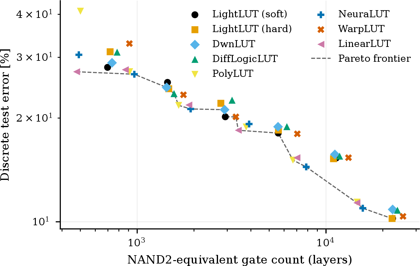
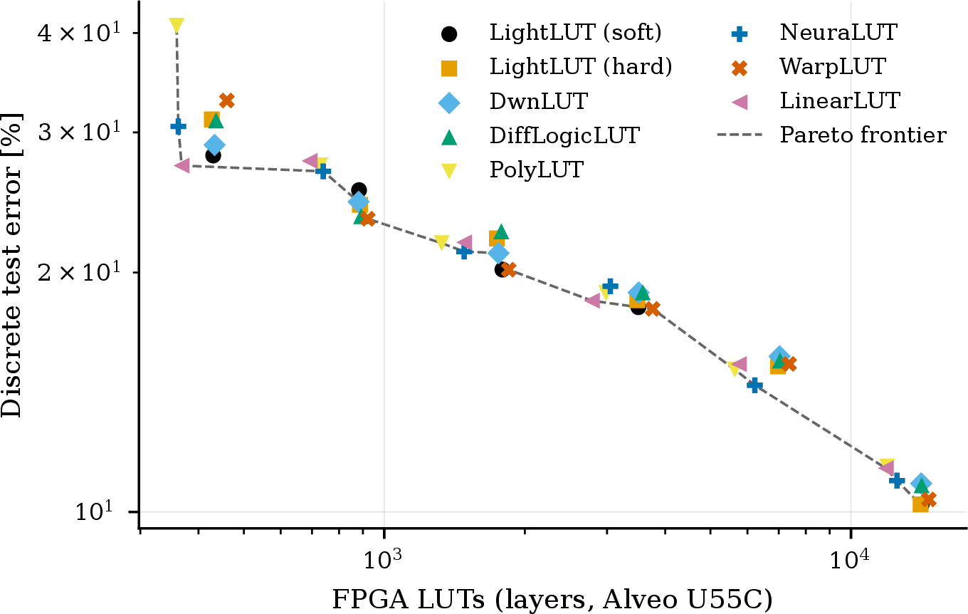
Figure 1: MNIST discrete test error versus hardware cost at matched \(n{=}2\) / \(b{=}4\), one series per node parameterization, swept over six widths, both axes log-scaled.
Error is evaluated in the HDL-matching forward mode (12.2.1), so the reported value equals the deployed-network error rate.. a — Cost on the layers submodule as standard-cell NAND2-equivalent gate
count (Yosys \(+\) Nangate \(45\) nm)., b — Cost as Vivado post-route LUT count of the layers submodule on the Alveo U55C target.
At \(w{=}32\)K the top cluster of 1 (LightLUT (soft/hard), WarpLUT, DwnLUT) sits within \({\sim}0.3\) pp of each other (\(96.88\)–\(97.11\) %), with PolyLUT and NeuraLUT trailing by \({\sim}0.6\)–\(0.9\) pp. Under matched \(n{=}2\) in 1 (a) the DiffLogic gap to the \(n{=}4\) cluster (of \({\sim}3.6\) pp in 1) narrows to \({\sim}2\) pp, so most of the DiffLogic deficit is a fan-in effect rather than a node-parameterization effect. The per-family error spread narrows with width (from \({\sim}1.5\times\) at the cheap end of the cost sweep to \({\sim}1.1\times\) at the wide end), so the choice of node parameterization matters most under tight hardware budgets.
5.2 Connectivity↩︎
We sweep six connectivity configurations (2): fixed routing with random or random-unique initialization, and learnable routing at candidate-pool sizes \(k \in \{4,\,8,\,16,\,\text{full layer}\}\). The ladder is \(w \in \{1{,}000,\,2{,}000,\,4{,}000\}\), narrower than the base ladder because the full-layer learnable cell does not fit at \(w{=}8\text{K}\) (11.1).
| Connectivity | Acc @ 1 K | Acc @ 2 K | Acc @ 4 K | NAND2-GE @ 1 K | LUTs @ 1 K |
|---|---|---|---|---|---|
| Learnable, full layer (-1) | \(79.10 \pm 0.88\) | \(81.18 \pm 0.92\) | \(81.47 \pm 0.18\) | \(\mathbf{3{,}908 \pm 4}\) | \(\mathbf{1{,}262 \pm 4}\) |
| Learnable, \(16\) candidates | \(\mathbf{86.19 \pm 0.27}\) | \(\mathbf{87.28 \pm 0.13}\) | \(\mathbf{88.84 \pm 0.06}\) | \(7{,}325 \pm 212\) | \(1{,}850 \pm 5\) |
| Learnable, \(8\) candidates | \(85.02 \pm 0.45\) | \(87.22 \pm 0.09\) | \(88.51 \pm 0.01\) | \(7{,}117 \pm 39\) | \(1{,}828 \pm 10\) |
| Learnable, \(4\) candidates | \(85.38 \pm 0.29\) | \(86.90 \pm 0.01\) | \(88.55 \pm 0.23\) | \(7{,}347 \pm 41\) | \(1{,}852 \pm 4\) |
| Fixed (random) | \(84.55 \pm 0.20\) | \(86.95 \pm 0.11\) | \(88.19 \pm 0.42\) | \(7{,}620 \pm 66\) | \(1{,}896 \pm 2\) |
| Fixed (random-unique) | \(84.10 \pm 0.10\) | \(86.62 \pm 0.16\) | \(87.97 \pm 0.01\) | \(7{,}755 \pm 29\) | \(1{,}917 \pm 9\) |
The full-layer learnable cell is the anomaly of this sweep. It drops to \(79.10\%\) at \(w{=}1\)K and \(81.47\%\) at \(w{=}4\)K, \(7\)–\(8\) pp below every bounded-candidate variant. With no candidate-pool bottleneck the softmax router mode-collapses: many slots converge on the same high-signal wires (a \({\sim}20\%\) reduction in distinct input wires per layer between the \(k{=}16\) and full-pool configurations, measured from the end-of-training argmax routing). When multiple LUT inputs tie to the same wire, the \(16\)-entry truth table reduces to an effective \(\leq\) \(3\)-input function and Yosys collapses the gate network accordingly, so the NAND2-GE reduction on that row is a hardware shadow of the same pathology visible in accuracy, not an efficiency gain. Among the non-pathological rows, fixed (random-unique) routing is within \({\sim}0.9\) pp of the best learnable variant at \(w{=}4\)K with no candidate-selection overhead.
5.3 Fan-in↩︎
We sweep \(n \in \{2,\,4,\,6\}\) across the three-width ladder with all other axes at the base architecture (3). Fan-in controls the per-node truth-table size (\(2^n\) entries) and is the axis where the standard-cell cost grows fastest, so this sweep maps the accuracy / cost knee that pins the cross-method comparison at \(n{=}4\) (10).
| Fan-in | Acc @ 8 K | Acc @ 16 K | Acc @ 32 K | NAND2-GE @ 8 K | LUTs @ 8 K |
|---|---|---|---|---|---|
| \(n{=}6\) | \(\mathbf{93.83 \pm 0.05}\) | \(\mathbf{96.44 \pm 0.01}\) | \(\mathbf{97.61 \pm 0.00}\) | \(248{,}588 \pm 779\) | \(16{,}134\) |
| \(n{=}4\) | \(91.13 \pm 0.02\) | \(94.85 \pm 0.03\) | \(97.12 \pm 0.03\) | \(60{,}673 \pm 125\) | \(15{,}250 \pm 14\) |
| \(n{=}2\) | \(84.69 \pm 0.08\) | \(89.58 \pm 0.11\) | \(93.75 \pm 0.06\) | \(\mathbf{11{,}358 \pm 192}\) | \(\mathbf{7{,}085 \pm 35}\) |
5.4 Encoder↩︎
We sweep three encoder families, each parameterized by a bit width \(b\) (4). The uniform and quantile (“distributive”) thermometers are evaluated at \(b \in \{4,\,8\}\). The binary-coded uniform quantizer at \(b \in \{2,\,8\}\). The low-bit point of the binary code isolates the regime where it outperforms the thermometers at half the wire count. \(b{=}8\) is common across all three for a matched high-bit comparison.
| Encoder (bits) | Acc @ 8 K | Acc @ 16 K | Acc @ 32 K | NAND2-GE @ 8 K | LUTs @ 8 K |
|---|---|---|---|---|---|
| DistributiveThermometer, \(b{=}4\) | \(\mathbf{91.26 \pm 0.01}\) | \(\mathbf{94.84 \pm 0.07}\) | \(\mathbf{97.15 \pm 0.03}\) | \(\mathbf{3{,}397}\) | \(\mathbf{1{,}568}\) |
| DistributiveThermometer, \(b{=}8\) | \(91.15 \pm 0.00\) | \(\mathbf{94.84 \pm 0.03}\) | \(97.09 \pm 0.01\) | \(7{,}690\) | \(3{,}136\) |
| Thermometer, \(b{=}4\) | \(90.39 \pm 0.05\) | \(94.19 \pm 0.12\) | \(96.89 \pm 0.09\) | \(14{,}112\) | \(5{,}488\) |
| Thermometer, \(b{=}8\) | \(90.42 \pm 0.17\) | \(94.27 \pm 0.08\) | \(96.81 \pm 0.09\) | \(35{,}221\) | \(10{,}976\) |
| UniformFixedPoint, \(b{=}2\) | \(89.78 \pm 0.07\) | \(93.51 \pm 0.04\) | \(96.38 \pm 0.02\) | \(13{,}034\) | \(3{,}920\) |
| UniformFixedPoint, \(b{=}8\) | \(88.59 \pm 0.05\) | \(92.61 \pm 0.10\) | \(95.55 \pm 0.04\) | — | \(12{,}544\) |
At matched nominal bit widths the quantile thermometer matches or beats the linear one by \({\sim}0.5\) pp on MNIST (consistent with [26]). Most of the gain and essentially all of the NAND2-GE reduction at \(b{=}4\) is an MNIST-specific threshold collapse rather than a real encoder win (11.3).
5.5 Head↩︎
We compare the popcount head with a DSP-backed quantized head (a \(c{\times}c\) signed matmul on the length-\(c\) group-sum vector with \(\text{wbits}{=}8\), so weights are \(\tanh\)-bounded during training and snapped to the signed integer grid \([-127,\,127]\) at inference, matching the integer MAC the emitter drops into the HDL) across the three-width ladder (5).
| Head | Acc @ 8 K | Acc @ 16 K | Acc @ 32 K | NAND2-GE @ 8 K | LUTs @ 8 K | DSPs @ 8 K |
|---|---|---|---|---|---|---|
| GroupedDSP | \(\mathbf{95.77 \pm 0.33}\) | \(\mathbf{97.42 \pm 0.08}\) | \(\mathbf{97.81 \pm 0.08}\) | \(75{,}666\) | \(12{,}028 \pm 224\) | \(39 \pm 1\) |
| GroupSum | \(91.14 \pm 0.00\) | \(94.84 \pm 0.02\) | \(97.12 \pm 0.04\) | \(\mathbf{59{,}080}\) | \(\mathbf{10{,}883}\) | \(\mathbf{0}\) |
6 Cross-method benchmark↩︎
We retrain the six gradient-trained priors (DiffLogic, PolyLUT, NeuraLUT, DWN, WARP-LUT, LILogicNet) inside the framework under the shared protocol of 4, each mapped via 6. To keep the comparison fair, the BitLogic best-of-space row pins fan-in to \(n{=}4\) and uses the popcount head across all rows. The rationale (and the remaining axis values from 5) is in 10.
| Dataset | Method | Acc @ 4 K | Acc @ 16 K | Acc @ 64 K | Published |
|---|---|---|---|---|---|
| MNIST | DWN | \(87.11 \pm 0.34\) | oom | oom | 97.80–98.77 |
| PolyLUT | \(86.24 \pm 0.09\) | \(91.61 \pm 0.17\) | \(96.22 \pm 0.00\) | 96.0–97.5 | |
| NeuraLUT | \(85.91 \pm 0.33\) | \(91.53 \pm 0.11\) | \(96.03 \pm 0.09\) | 96.0 | |
| LILogicNet | \(80.40 \pm 0.05\) | \(88.37 \pm 0.16\) | \(95.73 \pm 0.08\) | 97.96–98.95 | |
| WARP-LUT | \(76.40 \pm 0.22\) | \(85.89 \pm 0.10\) | \(93.59 \pm 0.04\) | — | |
| DiffLogic | \(75.92 \pm 0.30\) | \(85.89 \pm 0.03\) | \(93.68 \pm 0.05\) | 97.69–98.47 | |
| BitLogic best-of-space | \(\mathbf{88.94 \pm 0.14}\) | \(\mathbf{95.05 \pm 0.07}\) | \(\mathbf{97.84 \pm 0.04}\) | — | |
| F-MNIST | DWN | \(78.09 \pm 0.15\) | oom | oom | 89.01–89.12 |
| PolyLUT | \(74.65 \pm 0.24\) | \(83.08 \pm 0.28\) | \(87.00 \pm 0.12\) | — | |
| NeuraLUT | \(74.27 \pm 0.08\) | \(82.46 \pm 0.03\) | \(86.48 \pm 0.13\) | — | |
| LILogicNet | \(66.50 \pm 0.25\) | \(75.54 \pm 0.07\) | \(82.10 \pm 0.01\) | — | |
| WARP-LUT | \(65.65 \pm 0.38\) | \(75.36 \pm 0.12\) | \(83.00 \pm 0.05\) | — | |
| DiffLogic | \(65.42 \pm 0.05\) | \(75.40 \pm 0.04\) | \(82.89 \pm 0.12\) | 87.44 | |
| BitLogic best-of-space | \(\mathbf{78.38 \pm 0.14}\) | \(\mathbf{85.90 \pm 0.22}\) | \(\mathbf{89.16 \pm 0.08}\) | — | |
| CIFAR-10 | PolyLUT | \(36.95 \pm 0.02\) | \(46.16 \pm 0.01\) | \(53.02 \pm 0.16\) | — |
| NeuraLUT | \(36.73 \pm 0.02\) | \(44.38 \pm 0.33\) | \(47.30 \pm 0.65\) | — | |
| WARP-LUT | \(33.86 \pm 0.10\) | \(42.92 \pm 0.29\) | \(52.12 \pm 0.01\) | — | |
| LILogicNet | \(33.83 \pm 0.13\) | \(42.36 \pm 0.20\) | \(51.67 \pm 0.09\) | 55.11–60.98 | |
| DiffLogic | \(33.72 \pm 0.16\) | \(42.55 \pm 0.02\) | \(51.73 \pm 0.34\) | 51.27–62.14 | |
| DWN | oom | oom | oom | 57.42–57.51 | |
| BitLogic best-of-space | \(\mathbf{38.93 \pm 0.19}\) | \(\mathbf{49.22 \pm 0.26}\) | \(\mathbf{58.06 \pm 0.14}\) | — | |
| CIFAR-100 | PolyLUT | \(8.79 \pm 0.46\) | \(12.02 \pm 0.15\) | \(16.10 \pm 0.02\) | — |
| NeuraLUT | \(8.71 \pm 0.22\) | \(11.88 \pm 0.04\) | \(15.20 \pm 0.17\) | — | |
| LILogicNet | \(7.63 \pm 0.01\) | \(10.62 \pm 0.12\) | \(14.54 \pm 0.04\) | — | |
| DiffLogic | \(7.49 \pm 0.21\) | \(10.61 \pm 0.08\) | \(14.64 \pm 0.09\) | — | |
| WARP-LUT | \(7.00 \pm 0.04\) | \(10.46 \pm 0.00\) | \(14.43\) | — | |
| DWN | oom | oom | oom | — | |
| BitLogic best-of-space | \(\mathbf{10.19 \pm 0.06}\) | \(\mathbf{14.06 \pm 0.04}\) | \(\mathbf{18.82 \pm 0.09}\) | — |
Published numbers are reproduced from the cited works and are not protocol-matched. They reflect each paper’s own training budget and hardware conventions.
DiffLogic: [4].
NeuraLUT: [15]; the published cell quotes only the 2024 NeuraLUT recipe, which is the recipe the retrained row reproduces. NeuraLUT-Assemble 2025 [6] reports a higher MNIST accuracy of \(98.6\%\) but is a successor recipe not reproduced under the shared protocol ([sec:sec:appendix95reproducibility]).
DWN: [8]. The F-MNIST DiffLogic entry is a cross-fill from DWN’s Table 1, since F-MNIST is absent from DiffLogic’s own paper.
LILogicNet: [9].
DWN’s LR-DWN dense connectome uses the full-layer learnable fast-path, whose \(O(w^2)\) routing matrix exceeds the training GPU memory budget beyond \(w{\approx}4{,}000\); only the \(w{=}4{,}000\) cell is retrained, and the 10-bit thermometer input on CIFAR-10 / CIFAR-100 pushes even that out of budget. LILogicNet is retrained at its paper’s flagship Top-\(32\) connectivity and fits the full ladder.
Under the shared protocol, the best-of-space configuration wins every retrained (dataset, width) cell in which every compared prior fits the training budget: \(62\) of the \(72\) (\(4\) datasets \({\times}\,3\) widths \({\times}\,6\) priors) cells in ¿tbl:tab:best95of95space?; the remaining \(10\) are DWN oom entries (note [f]) and are not part of that count. At \(w{=}64\)K the best-of-space reaches \(97.84 / 89.16 / 58.06 / 18.82\) % on MNIST / F-MNIST / CIFAR-10 / CIFAR-100; the two largest margins are \(\sim\)1.6 pp over PolyLUT on MNIST and \(\sim\)5 pp over PolyLUT on CIFAR-10.
Where the published row exceeds the retrained row by more than \({\sim}1\) pp (DWN on MNIST: \(97.80\)–\(98.77\) vs.retrained \(87.11\); LILogicNet on MNIST: \(97.96\)–\(98.95\) vs.retrained \(95.73\) at \(w{=}64\)K; NeuraLUT-Assemble on MNIST, \(98.6\), not retrained), the gap traces to a method-specific calibration, pruning, or thresholding pipeline that the shared protocol disables (full list in 10). Under the shared protocol, the design-space coordinates of the BitLogic best-of-space dominate every retrained prior at every width that fits the training budget.
7 Hardware deployment↩︎
One checkpoint emits to three backends from a single framework: a bit-packed GPU forward path that processes \(64\) samples per \(64\)-bit operation, synthesizable SystemVerilog placed and routed by Vivado on two FPGA targets (Alveo U55C, Zynq UltraScale+ XCZU7EV), and a flat Yosys netlist against Nangate \(45\) nm as a target-independent ASIC proxy. The GPU deployment runs on three consumer cards (12). We deploy the MNIST winner of ¿tbl:tab:best95of95space? at \(w{=}4{,}000\), the widest cell our build host fits. Wider cells extrapolate linearly at unchanged timing (12.5). FPGA numbers are Vivado post-route, with Verilator confirming bit-exact agreement against the Python reference on the full MNIST test set.
7.0.0.1 Emission modes.
Each FPGA row picks one of three modes: max throughput (parallel encoder/head, fully pipelined, \(\mathrm{II}{=}1\)), lowest latency (parallel encoder/head, no pipelining), and fewest resources (parallel encoder, combinational layers, iterative popcount head over \(\mathrm{II}{=}c\) cycles). On the MNIST winner only head iteration pays back. The per-knob breakdown is in 11.2.
7.0.0.2 Cross-platform headline.
¿tbl:tab:hardware95evaluation? reports \(F_\text{max}\), latency, throughput, power, and energy per sample across the three FPGA modes, both targets, and three GPU references at two batch sizes. All rows share the same checkpoint, so accuracy is identical (\(88.79\%\) on the full MNIST test set, within the two-seed \(88.94\pm0.14\%\) band of ¿tbl:tab:best95of95space?). Resource footprints are in [tab:hardware_resources_fpga,tab:hardware_resources_asic,tab:hardware_resources_gpu].
@ l l r r r r r @ Platform & Mode & \(F_\text{max}\) & Lat & Tput & Power &
Energy
& & (MHz) & (ns) & (kSmp/s) & (W) & (nJ/smp)
& batchsize 64 & \(2{,}115\) & \(115{,}712\) & \(550.0\) & \(130.67\) & \(2{,}287{,}786\)
& batchsize 1024 & \(2{,}115\) & \(116{,}736\) & \(8663.7\) & \(291.42\) & \(319{,}425\)
& batchsize 64 & \(2{,}100\) & \(114{,}224\) & \(553.5\) & \(58.02\) & \(1{,}014{,}773\)
& batchsize 1024 & \(2{,}100\) & \(146{,}656\) & \(6984.6\) & \(199.60\) & \(227{,}080\)
& batchsize 64 & \(2{,}100\) & \(118{,}784\) & \(533.0\) & \(72.49\) & \(1{,}273{,}177\)
& batchsize 1024 & \(2{,}100\) & \(135{,}088\) & \(7587.7\) & \(218.91\) & \(246{,}347\)
& max throughput & \(126.6\) & \(40\) & \(126566.3\) & \(3.40\) & \(27\)
& lowest latency & \(84.4\) & \(12\) & \(84359.7\) & \(3.34\) & \(40\)
& fewest resources & \(110.8\) & \(99\) & \(10069.7\) & \(3.37\) & \(335\)
& max throughput & \(127.2\) & \(39\) & \(127177.9\) & \(0.72\) & \(6\)
& lowest latency & \(84.7\) & \(12\) & \(84652.5\) & \(0.66\) & \(8\)
& fewest resources & \(115.8\) & \(95\) & \(10528.0\) & \(0.68\) & \(65\)
Ultra96 (ZUS+ ZCU3EG) & FINN-R MLP-4 (MNIST) [18] & \(300.0\) & — & \(851.7\) & \(11.80\) & \(13{,}856\)
PYNQ-Z1 (Zynq-7020) & FINN-R MLP-4 (MNIST) [18] & \(100.0\) & — & \(162.3\) & \(2.50\) & \(15{,}400\)
Pynq-Z2 (Zynq-7020) & ResNet-V1 hls4ml (CIFAR-10) [29] & — & \(27{,}300{,}000\) & — & — & \(44{,}330{,}000\)
Pynq-Z2 (Zynq-7020) & CNV-W1A1 FINN (CIFAR-10) [29] & — & \(1{,}500{,}000\) & — & — & \(2{,}535{,}000\)
The three modes span a clear resource–throughput trade-off: max-throughput buys \({\sim}1.5\times\) throughput for three orders of magnitude more flip-flops, while fewest resources cuts LUTs by \({\sim}1.5\times\). The pipelined implementation reaches \(126.6\) MSamp/s (U55C) and \(127.2\) MSamp/s (XCZU7EV), about \(15\times\) the RTX 3090 and \(17\)–\(18\times\) the Turing cards, at \(6\)–\(27\) nJ per sample, four to five orders of magnitude below GPU. The published FPGA numbers in the bottom row group of ¿tbl:tab:hardware95evaluation? are not a fair comparison, see 12.6.
8 Discussion, limitations, and outlook↩︎
8.0.0.1 What the sweep taught us.
Two axes give clean signal and two surface structural surprises. Fan-in is the single largest lever: the \(n{=}2{\to}4\) step alone explains most of DiffLogic’s gap to the \(n{=}4\) cluster, and the matched-\(n{=}2\) figures ([fig:node_rank2_nand,fig:node_rank2_lut]) narrow that gap from \({\sim}3.6\) pp to \({\sim}2\) pp. Once \(n\) is fixed, the top node cluster (LightLUT, WarpLUT, DwnLUT) converges within \({\sim}0.3\) pp at \(w{=}32\)K (1), so the relaxation family matters much less than the literature suggests. Full-layer learnable connectivity mode-collapses \(7\)–\(8\) pp below every bounded-candidate variant (5.2). The apparent NAND2-GE win on that row is a hardware shadow of the pathology, not an efficiency gain. The quantile thermometer’s lead on MNIST is largely an artefact of an MNIST-specific threshold collapse (11.3), not encoder dominance: \((\text{pixel}>0)\) already carries most of the MNIST signal.
8.0.0.2 Where the parameterization win shows up.
The per-axis ranking of 1 compares node parameterizations at fixed width, and the best-of-space combination of ¿tbl:tab:best95of95space? amplifies that ranking. On GPU this translates directly into runtime, since cost is set by parameter count and width. [fig:node_rank2_nand,fig:node_rank2_lut] re-project the same axis against ASIC NAND2-equivalent gate count and FPGA LUT count, and the per-family error spread shrinks from about \(1.5\times\) at the cheap end of the cost sweep to about \(1.1\times\) at the wide end. On those fabric backends the node-parameterization choice is therefore largely orthogonal: any of the node parameterizations sits within about \(1.1\times\) of any other at deployment-relevant cost. The accuracy headroom from picking the best-of-space combination matters most when parameter count drives runtime cost, that is, on GPU.
8.0.0.3 Depth, the open sixth axis.
Every configuration we evaluate is two layers deep, and we deliberately did not sweep depth. Randomly-initialized LUT stacks lose accuracy rapidly with depth (pilot runs show the soft-vs-hard training gap widening and gradients vanishing through stacked saturating relaxations), and every known remedy introduces a new axis: residual identity initialization [21] and fixed-connectivity routing both mitigate the collapse. We flag depth as the next unsolved axis rather than the next parameter.
8.0.0.4 Extensibility.
The five axes are independently swappable at the layer level: a reader with a new node, encoder, or connectivity rule can rerun 5 with one config change and measure the new axis against the whole retrained slate. Whole-model topology is fixed in the current release (dense logic layers plus a small set of heads and encoders), but the extension points are clear: convolutional logic layers [21], residual/skip variants, and recurrent LUT layers [30] all exist in isolation. The natural next step is to make each a first-class axis so the same protocol-matched comparison applies. The framework is not bound to image classification, and extending it to other tasks is feasible.
8.0.0.5 Outlook.
The pipelined FPGA deployment of 7 already runs at sustained throughput high enough that on the edge the sensor and downstream pipeline, not the network, become the bottleneck. Whether this profile extends to attention, residual, or recurrent LUT-native networks at LLM scale is the open question BitLogic is meant to enable: every modern neural-network success story (attention, residual learning, convolution, recurrence) has been written in the floating-point idiom, and each needs a LUT-native counterpart before the edge and serving efficiencies reported here transfer to serving-scale workloads. The five axes we swept are the feedforward base case. The next axes are topology, depth, and task.
9 Conclusion↩︎
Casting every gradient-based feedforward LUT method as a point in one five-axis design space and sweeping each axis under a shared protocol yields a new best-of-space model, a combination no prior paper has trained, that matches or exceeds every retrained baseline on \(62\) of the \(72\) (dataset, width, prior) cells of ¿tbl:tab:best95of95space? across MNIST, Fashion-MNIST, CIFAR-10, and CIFAR-100. The same checkpoint, emitted to bit-exact SystemVerilog and to a standard-cell netlist, reaches the throughput and energy figures reported in 7. While this best-of-space accuracy headroom translates into a visible GPU runtime advantage, on FPGA and ASIC the cost-versus-accuracy curves of [fig:node_rank2_nand,fig:node_rank2_lut] cluster across all node parameterizations, so the parameterization choice mainly matters for GPU efficiency.
LUT-based networks push inference onto extremely low-energy hardware, which is broadly positive for the energy footprint of deployed machine-learning systems. Extending the framework beyond image classification is a natural next step.
10 Reproducibility: initialization, prior-method mapping, sweep recipes↩︎
This appendix supplements the training protocol of 4 with initialization detail, the mapping of each prior method onto the five design-space axes used for the retrained rows of ¿tbl:tab:best95of95space?, the axis constraints that pin those BitLogic rows at \(n{=}4\) and the popcount head, the fidelity scope of the retrained column, the per-experiment sweep recipes, and the training-cost numbers. The hardware pipeline (bit-packed inference, HDL emission, Vivado post-route flow, Yosys \(+\) Nangate \(45\) nm standard-cell synthesis) is deferred to 12.
10.0.0.1 Initialization.
Fixed routing draws its index tensor once per layer as either i.i.d.random or random-unique. Learnable routing draws the candidate-pool mask uniformly and initializes the per-slot routing logits to zero, so the expected selection is uniform across
candidates at the first step. Node parameters are drawn from a zero-mean Gaussian (every parametrization’s weight_init="random" default). The library also exposes an opt-in residual-anchor init that biases each node toward pass-through of its
last input, but it is not enabled in any sweep reported here. Quantile-thermometer thresholds are fit once from the empirical pixel quantiles on the training split. The linear thermometer uses equispaced thresholds in the value range.
10.0.0.2 Seeds.
Seeds \(\in \{0, 1\}\) drive torch, NumPy, and the 90/10 train/validation split. Every per-axis and cross-method experiment reports mean \(\pm\) std over both seeds. The rank-2 node sweep ([fig:node_rank2_nand,fig:node_rank2_lut]) is single-seed by design: it is a cost-vs-accuracy projection rather than a mean comparison, and the within-seed cost spread is already dominated by the width sweep itself.
10.0.0.3 Prior-method mapping.
Each prior method in ¿tbl:tab:best95of95space? corresponds to the design-space coordinates listed in 6 and is trained at three widths \(w \in \{4{,}000,\,16{,}000,\,64{,}000\}\) on each of the four datasets. Two exceptions: DWN’s LR-DWN dense connectome uses the full-layer learnable fast-path, whose \(O(w^2)\) routing matrix exceeds the GPU memory budget beyond \(w{\approx}4{,}000\), so DWN is retrained at \(w{=}4{,}000\) only on MNIST and Fashion-MNIST and is oom at every width on CIFAR-10 / CIFAR-100 (where its \(10\)-bit thermometer further inflates the input tensor). LILogicNet is retrained at its paper’s flagship Top-\(32\) connectivity (the 2Top32 variant, [9] Table 3), whose \(O(w{\cdot}32)\) routing matrix fits the full ladder. “Learnable(\(k\))” denotes learnable routing with candidate-pool size \(k\), and \(k{=}{-}1\) denotes the full-layer fast-path. Encoder family and per-dataset bit count \(b\) come from each method’s paper. Missing datasets use a nearest-neighbour extrapolation (grayscale \(\leftrightarrow\) MNIST, RGB \(\leftrightarrow\) CIFAR-10). For DiffLogic, \(b{=}1\) on MNIST reproduces the paper’s binarized-MNIST single threshold at \(0.5\), and \(b{=}3\) on CIFAR-10 reproduces the “small” row of their Table 5 (fixed per-channel thresholds \(\{0.25, 0.5, 0.75\}\)). The \(31\)-threshold “large” CIFAR-10 variant is not retrained.
10.0.0.4 Axis constraints in the cross-method comparison.
Two of the five axes are held fixed across all BitLogic rows of ¿tbl:tab:best95of95space? rather than taken from the per-axis winners of 5. Fan-in is pinned to \(n{=}4\) because (i) the majority of retrained priors (PolyLUT, NeuraLUT, and DWN) natively evaluate at rank \(4\), and (ii) the fan-in sweep (3) shows accuracy improves faster with width than with rank on the prior-method ladder, so \(n{=}4\) keeps most priors at their native rank while retaining width headroom. DiffLogic, WARP-LUT, and LILogicNet, which default to \(n{=}2\) in their own papers, therefore sit at rank \(4\) here as a controlled design-space coordinate, not an accidental mismatch. The head is pinned to the popcount GroupSum so the comparison stays pure LUT-only: a DSP-backed head would add a quantized matrix-multiply that no prior method uses, turning the table into a hybrid LUT\(+\)DSP vs.LUT-only contest. The remaining three axes (node parameterization, connectivity, encoder) are set to the per-axis winners of [tab:rq_node,tab:rq_conn,tab:rq_encoder].
10.0.0.5 Scope of the prior-method reproduction.
6 aligns each retrained baseline with its paper along the five design-space axes. This is an axis-level alignment, not a full re-implementation. The protocol of 4 is shared across all rows, so the comparison is controlled for everything except the design-space choices, and method-specific machinery is intentionally out of scope. PolyLUT-2025’s hardware-aware structured-pruning pipeline (dense pre-train with exponential-\(\ell_1\) group regularizer, top-\(k\) prune, retrain from reinitialized weights, [5]) and NeuraLUT-Assemble’s successor recipe [6] are not reproduced, so the PolyLUT and NeuraLUT rows use the fixed (random) sparsity of the 2023 / 2024 originals rather than learned connectivity. DWN’s bespoke schedule and quantile-thermometer calibration [8] are replaced by the shared recipe. LILogicNet’s flagship Top-\(32\) learnable connectivity [9] is kept verbatim, but its dataset-specific binarization thresholds are replaced by linear thermometer thresholds at \(i/(b{+}1)\). WARP-LUT’s full residual convolutional block [7] is replaced by the flat dense backbone used by every other row. The resulting numbers should therefore be read as “each method’s parameterization and connection scheme, trained under BitLogic’s uniform recipe”, not as a reproduction of each headline number.
| Encoder bits \(b\) | ||||||||
|---|---|---|---|---|---|---|---|---|
| 6-9 Method | Node parameterization | Connections | \(n\) | Encoder | MNIST | F-MNIST | CIFAR-10 | CIFAR-100 |
| DiffLogic | softmax over 16 ops | fixed (random) | 2 | linear thermometer | 1 | \(1^\dagger\) | 3 | \(3^\dagger\) |
| PolyLUT | degree-\(d\) polynomial | fixed (random) | 4 | binary-coded quantizer | 2 | \(2^\dagger\) | \(2^\dagger\) | \(2^\dagger\) |
| NeuraLUT | MLP per neuron | fixed (random) | 4 | binary-coded quantizer | 2 | \(2^\dagger\) | \(2^\dagger\) | \(2^\dagger\) |
| DWN | full truth table (EFD) | learnable(\(-1\)) | 6 | quantile thermometer | 3 | 7 | 10 | \(10^\dagger\) |
| WARP-LUT | Walsh basis | fixed (random) | 2 | linear thermometer | \(1^\dagger\) | \(1^\dagger\) | 3 | \(3^\dagger\) |
| LILogicNet | softmax over 16 ops | learnable(\(32\)) | 2 | linear thermometer | 1 | \(1^\dagger\) | 7 | \(7^\dagger\) |
| BitLogic best-of-space | LightLUT (soft) | learnable(\(16\)) | 4 | quantile thermometer | 4 | 4 | 4 | 4 |
10.0.0.6 Per-experiment recipes.
7 lists each paper element with the axis it sweeps, the swept values, and the width ladder. Standard-cell synthesis is not invoked for the per-axis sweeps or the cross-method comparison. Hardware cost is reserved for the rank-2 node figures ([fig:node_rank2_nand,fig:node_rank2_lut]) and the deployment case study (7).
| Element | Swept axis and values | Width ladder |
|---|---|---|
| [tab:rq95node] | node: {LightLUT (soft, hard), DwnLUT, PolyLUT, NeuraLUT, WarpLUT, LinearLUT, DiffLogic} | \(\{8,16,32\}\) K |
| [tab:rq95conn] | connectivity: {fixed (random), fixed (random-unique), learnable(\(k\)) for \(k{\in}\{4,8,16,-1\}\)} | \(\{1,2,4\}\) K |
| [tab:rq95fanin] | fan-in: \(n \in \{2, 4, 6\}\) | \(\{8,16,32\}\) K |
| [tab:rq95encoder] | encoder \(\times\) bits: {uniform, quantile}\(\times\), binary\(\times\) | \(\{8,16,32\}\) K |
| [tab:rq95head] | head: {popcount, DSP-backed (\(\text{wbits}{=}8\))} | \(\{8,16,32\}\) K |
| [tab:best95of95space] | BitLogic best + 6 prior methods ([tab:prior95mapping]), \(\times\) 4 datasets | \(\{4,16,64\}\) K |
| [fig:node_rank2_nand,fig:node_rank2_lut] | node sweep at rank-2 / \(b{=}4\) / learnable(\(8\)) / popcount, single seed | \(\{0.5,1,2,4,8,16\}\) K |
| [tab:hardware95evaluation]–[tab:hardware95resources95asic] | deployment case study driven by the MNIST winner of [tab:best95of95space] | \(w{=}4\) K |
The BitLogic cells in ¿tbl:tab:best95of95space? use the best-of-space configuration identified by the per-axis winners of 5: LightLUT (soft) nodes, learnable routing with \(k{=}16\) candidates, \(n{=}4\), a \(b{=}4\) distributive thermometer, and a popcount head.
10.0.0.7 Training cost.
8 reports per-parameterization wall-clock and peak GPU memory at the largest node-sweep width (\(w{=}32{,}000\)). Training runs on a shared heterogeneous GPU cluster whose scheduler allocates whichever device is free, so seeds of the same cell routinely land on different silicon. Seconds per epoch scale roughly linearly with width. Within each row the two seeds are grouped by host GPU rather than averaged across dissimilar cards.
| Parametrization | GPU host(s) | Trainable params | s / epoch | Total (min) | Peak GPU (GB) |
|---|---|---|---|---|---|
| LightLUT (hard) | RTX 3090 / TITAN RTX | \(3{,}072{,}000\) | \(35.50\) / \(34.07\) | \(59.16\) / \(56.78\) | \(2.535\) / \(2.535\) |
| LightLUT (soft) | RTX 3090 | \(3{,}072{,}000\) | \(26.93\) | \(44.89\) | \(2.535\) |
| DwnLUT | RTX 3090 / TITAN RTX | \(3{,}072{,}000\) | \(49.31\) / \(26.90\) | \(82.18\) / \(44.83\) | \(1.806\) / \(1.806\) |
| DiffLogicLUT (\(n{=}2\)) | RTX 3090 / TITAN RTX | \(2{,}048{,}000\) | \(\mathbf{15.04}\) / \(19.51\) | \(\mathbf{25.07}\) / \(32.52\) | \(\mathbf{0.936}\) / \(\mathbf{0.936}\) |
| PolyLUT | RTX 2080 Ti | \(4{,}288{,}000\) | \(50.28\) | \(83.80\) | \(3.320\) |
| NeuraLUT | RTX 3090 / TITAN RTX | \(5{,}184{,}000\) | \(42.60\) / \(36.63\) | \(71.00\) / \(61.05\) | \(2.220\) / \(2.220\) |
| WarpLUT | RTX 2080 Ti | \(3{,}072{,}000\) | \(44.11\) | \(73.51\) | \(2.451\) |
| LinearLUT | RTX 3090 | \(2{,}368{,}000\) | \(37.47\) | \(62.45\) | \(1.852\) |
11 Extended sweep data↩︎
This appendix collects the experimental detail that is orthogonal to the narrative of [sec:sweep,sec:benchmark,sec:hardware_evaluation] but that the reader may need when interrogating the headline numbers: why each sweep uses the width ladder it does, which axes are held fixed in the cross-method comparison and why, and which emitter knobs pay back on the MNIST winner in 7.
11.1 Width ladders↩︎
The per-axis sweeps are reported at three widths per axis so that axis signal is separable from width scaling. The node, fan-in, encoder, and head sweeps of 5 use the base ladder \(w \in \{8{,}000,\,16{,}000,\,32{,}000\}\), centred on the \(w{=}16{,}000\) base cell. The connectivity sweep uses the smaller ladder \(w \in \{1{,}000,\,2{,}000,\,4{,}000\}\) because its full-layer learnable cell materializes a dense \(w{\times}w\) routing matrix per layer and does not fit at the 8 K base within our training GPU memory budget. The relative ordering of the bounded-candidate rows at that ladder carries over to the wider ladder when re-run, but the full-layer cell is not reachable above \(w{\approx}4{,}000\) under this recipe. The cross-method comparison of ¿tbl:tab:best95of95space? uses the wider ladder \(w \in \{4{,}000,\,16{,}000,\,64{,}000\}\) for every row that fits, so the deployment regime is visible. DWN’s LR-DWN dense connectome inherits the same full-layer fast-path and is retrained at \(w{=}4{,}000\) only, with wider cells marked oom in the same sense.
11.2 Cost-model asymmetry of the FPGA emitter↩︎
The fewest resources design point of 7 is a selected combination of the emitter knobs, not a blanket “iterate everything” switch. Each knob was measured on the MNIST winner and kept only when it actually reduces whole-model cost.
11.2.0.1 Head iteration wins on both cost models.
Time-sharing the per-class popcount and argmax reduces the head from \({\sim}5{,}170\) LUTs (\({\sim}29.5\) k NAND2-eq) to \({\sim}2{,}120\) LUTs (\({\sim}7.6\) k NAND2-eq) for \(k{=}10\) classes. The per-class reduction is expensive enough that time-sharing it still wins after paying for the counter and output-latch flip-flops.
11.2.0.2 Encoder iteration loses at small input scales.
The parallel encoder for the MNIST winner is already cheap: \(s{\cdot}b = 784{\cdot}4 = 3{,}136\) thermometer bits, \(3{,}397\) NAND2-eq total, because each channel is a short comparator chain. Replacing it with a time-shared comparator over \(784\) slots requires a \(3{,}136\)-bit output register whose standard-cell cost alone (\({\sim}15{,}680\) NAND2-eq at \({\sim}5\) NAND2 per flip-flop) dominates the combinational savings, and iterative emission measures \({\sim}5.8\times\) worse end-to-end. On FPGA the flip-flops pack into slice positions already bundled with the LUTs, so the register cost is near-zero in slice-LUT accounting, but the input-gather multiplexer still drives the encoder LUT count up from \(1{,}568\) to \(3{,}301\). At larger input scales the ratio flips, and the MNIST winner is simply too encoder-small for iteration to pay back.
11.2.0.3 Layer iteration loses on random-wiring LUT fabrics.
Each LUT‘s \(n\) inputs are independently learned indices into the prior layer’s output (no spatial locality, no convolutional structure), so a time-shared layer fabric needs a per-neuron \(w{:}1\) multiplexer on each of its \(n\) inputs to switch between the two layers’ id tensors. At \(w{=}4{,}000\) and \(n{=}4\) that gather cost is comparable to the LUT-lookup itself, and adding a \(4{,}000\)-bit inter-layer register tips the balance. Layer emission therefore stays combinational.
The selected combination (parallel encoder, combinational layers, iterative head) minimizes both FPGA LUT count and Nangate 45 nm gate count on this model. The asymmetry is intrinsic to the interaction between emitter knobs and cost model, not a defect of any one knob. A bigger encoder or a structured connectome would flip these verdicts.
11.3 MNIST-specific encoder collapse↩︎
The NAND2-eq column of 4 needs a caveat: the DistributiveThermometer row synthesizes to a quarter of the Thermometer row at matched nominal bit widths (\({\sim}3{,}400\) vs.\({\sim}14{,}100\) at \(b{=}4\)), but these two encoders are not operating at matched effective bit widths on MNIST. Quantile thresholds are fit over the globally flattened training pixel distribution, which on MNIST has a point mass at zero exceeding the \(88\) % quantile. Inspecting the fitted checkpoint: at \(b{=}4\) all four thresholds are \(0.0\), and at \(b{=}8\) seven of the eight are \(0.0\) with the last at \(\approx 0.706\). The ladder therefore collapses: at \(b{=}4\) every bit is the same \((\text{pixel} > 0)\) comparison and the encoder is effectively \(1\)-bit, while at \(b{=}8\) it is effectively \(2\)-bit. Yosys hashes the identical per-bit expressions and emits one comparator per pixel. The linear thermometer places its thresholds uniformly in the value range and does not collapse on MNIST, so the two rows compare a genuine \(b\)-bit code against an effectively \(1/2\)-bit code. That the collapsed variant still leads on accuracy simply confirms that \((\text{pixel} > 0)\) already carries most of the MNIST signal.
12 Hardware evaluation methodology (GPU, FPGA, ASIC)↩︎
This appendix documents how every hardware number in 7 is produced: which static-analysis pass populates each column, how the GPU, FPGA, and ASIC paths are made comparable, and how the per-mode cycle budget combines with Vivado’s achieved period to yield the reported latency and throughput. A short closing subsection covers the width-scaling extrapolation that licences the single-width hardware report.
No physical FPGA board is programmed for any reported row: the FPGA numbers come from post-place-and-route Vivado reports or, where Vivado’s placer bails on wide-port designs, from post-optimization estimates (made precise below). Training runs on a shared heterogeneous GPU cluster (RTX 3090, RTX 2080 Ti, or Titan RTX) under PyTorch 2.x on CUDA 12. The exact card, driver, and host CPU per seed are recorded in the run record and unioned into the GPU host(s) column of 8 at aggregation time.
12.1 GPU methodology↩︎
GPU latency, throughput, and energy are measured against a bit-packed inference path (64 samples per 64-bit operation) that is graph-captured into a single CUDA replay. The remainder of this subsection describes the path’s construction, the compiled forward, the timing protocol, the telemetry sampler, and the correctness anchor that ties GPU accuracy to the Python evaluation.
12.1.0.1 Bit-packed inference.
The GPU rows of ¿tbl:tab:hardware95evaluation? and every accuracy number in [sec:sweep,sec:benchmark] use a bit-packed inference path, not the eager forward. At construction the path walks each layer once, extracts the discrete \(2^n\)-entry truth table plus the per-node routing indices, and normalizes them to a common LUT input bit order. At inference, \(64\) samples along the batch dimension are packed into a single 64-bit integer, and each layer’s LUT evaluation becomes a bitwise op on packed tensors that processes \(64\) samples per op. The encoder and head remain in floating point. The packed output is bit-exact with the eager discrete forward and, by construction, with the emitted SystemVerilog (12.2.2). On a modern GPU it is roughly one to two orders of magnitude faster than the eager path.
12.1.0.2 Compiled forward.
The bit-packed module is wrapped in PyTorch’s inference mode and compiled with graph capture, fusing the per-layer pack, bitwise-LUT, and unpack kernels into a single replayable graph. This is the closest GPU analogue of the emitted SystemVerilog: one submitted unit of work per sample batch, no per-iteration driver round-trips. The batch is moved to the device once before timing, so no host-to-device transfers and no dataloader work enter the timed region.
12.1.0.3 Timing protocol.
Per-iteration latency is measured with CUDA events placed as barriers between back-to-back forwards. Warmup fires the forward without host synchronization until both an iteration-count floor (\(500\) iters) and a wall-clock floor (\(5\) s) are met, long enough for the card’s DVFS controller to settle out of its idle P-state, which matters on Turing consumer silicon. A single device synchronization then gates entry to the timed region, where the driver records \(N{+}1\) barrier events and submits \(N{=}5{,}000\) back-to-back forwards. Per-iteration latency is recovered from the event-to-event elapsed time. Throughput is \(N\cdot\text{batch}\) divided by a wall-clock bracket around the loop. Each device is benchmarked at two batch sizes (\(64\) and \(1024\)) so small-batch and sustained regimes are both visible.
12.1.0.4 Energy and clock telemetry.
A background NVML sampler polls power, SM clock, memory clock, and junction temperature at \(10\) Hz over the timed region. Power samples are integrated to joules with the trapezoidal rule. Clocks and temperature are summarized as min/mean/max. The card’s nominal boost ceiling is read once at startup, and a row whose observed peak SM clock sits more than \(10\%\) below that ceiling is flagged as DVFS-limited rather than compute-bound, so an artificially depressed clock is not silently read as a latency win.
12.1.0.5 Correctness anchor.
Before timing, the driver compares a one-batch eager forward against the bit-packed forward: exact equality for LightLUT checkpoints, a \(10^{-4}\) element-wise tolerance for softer parameterizations. Test accuracy through the bit-packed path is recorded alongside the timing numbers, so every GPU row carries its own correctness check and is bit-exact with the Python accuracy reported by [sec:sweep,sec:benchmark].
| Platform | Mode | Memory (MB) |
|---|---|---|
| RTX 3090 / RTX 2080 Ti / TITAN RTX | batchsize 64 | \(7.27\) |
| batchsize 1024 | \(10.15\) |
12.2 FPGA methodology↩︎
The HDL emitter writes one synthesizable SystemVerilog top module per emission mode and records its cycle budget \((D, \mathrm{II}, C)\), i.e.pipeline depth, initiation interval, and cycles-per-sample. Vivado then turns those constants and the achieved clock period into the latency, throughput, and resource numbers reported in [tab:hardware_evaluation,tab:hardware_resources_fpga].
12.2.1 HDL export and emission modes↩︎
Every FPGA number originates from a single trained checkpoint. The HDL emitter extracts each layer’s truth table and routing indices and writes synthesizable SystemVerilog. The top module inlines the full forward path (encoder comparators, logic layers, and head) as a single block, with quantized encoder code as input and predicted class index as output, so every downstream resource number covers the whole model end-to-end.
Three orthogonal emitter options select the three modes of 7: encoder style (parallel vs. iterative), head style (parallel vs.iterative), and three independent pipeline flags (encoder / logic layers / head). Each mode fixes a deterministic cycle budget \((D, \mathrm{II}, C)\) that the emitter records before any synthesis. For an \(L\)-layer stack, the core pipeline depth is \[D_\text{core} = \mathbb{1}_{\text{pipe\_enc}} + L\cdot\mathbb{1}_{\text{pipe\_layers}} + \mathbb{1}_{\text{pipe\_head}}.\]
Max throughput. Parallel encoder and head, with pipeline flip-flops at the encoder, every logic layer, and the head. \(D_\text{core}{=}4\) on the two-layer MNIST winner, with \(\mathrm{II}{=}1\) (one sample in, one sample out per cycle).
Lowest latency. Parallel encoder and head, pipelining off, so the core datapath is purely combinational (\(D_\text{core}{=}0\)). The shim wraps it as a single flop-to-flop stage for Vivado.
Fewest resources. Parallel encoder, combinational logic layers, iterative popcount head. A single shared popcount/argmax updater walks the \(c\) output classes sequentially, so \(\mathrm{II}_\text{core}{=}c\) (\(c{=}10\) on MNIST). Iterating the encoder or layers is a net regression on random-wiring LUT networks at MNIST scale (11.2).
The full-module rows additionally enable the BRAM-backed I/O shim (12.2.3.1), whose output register adds exactly one flop-to-flop stage. The cycle-budget calculator folds that \(+1\) into \(D\), \(\mathrm{II}\), and \(C\) when the shim is enabled, so the table renderer needs no shim-specific branch.
12.2.2 HDL fidelity↩︎
For every checkpoint used in 7 we run an equivalence check on the full test split: Verilator compiles the emitted SystemVerilog with an auto-generated byte-streaming harness, each test sample is piped through the binary, and its one-byte class-index output is compared against the bit-packed inference argmax. All rows across all three emission modes on both FPGA targets report agreement \(1.0\) on the full test set, certifying that every FPGA accuracy number is bit-exact with the reported Python evaluation. The same check runs per seed in the per-axis sweeps on a \(1{,}000\)-sample subsample for speed.
12.2.3 Vivado deployment↩︎
The two FPGA targets, an Alveo U55C (part xcu55c-fsvh2892-2L-e) and a Zynq UltraScale+ XCZU7EV (part xczu7ev-ffvc1156-2-e), share the UltraScale+ 6-LUT primitive (so resource counts are directly comparable) and differ in capacity (\({\sim}1.3\) M LUTs on U55C vs. \({\sim}230\) k on the XCZU7EV). Both run the same non-project Vivado 2024.2 flow, synthesizing out-of-context to skip I/O buffer insertion.
12.2.3.1 BRAM-backed I/O shim.
The MNIST winner’s \(784\times 8 = 6{,}272\)-bit encoder input does not fit either part: the count is far above any Xilinx package’s pin budget and trips Vivado’s placer IO-rule check before placement even begins. To make the design synthesizable and make the reported numbers reflect real evaluation rather than constant-folded ghosts, the emitter wraps the core in a thin registered shim with a small pin footprint (clock, reset, class-id). A four-entry BRAM-inferred ROM holds distinct sample bit patterns. On every cycle the next sample is buffered into a wide input register driving the core, and the core’s output is captured one cycle later into an output register. Because real, varying sample data is clocked through the network each cycle, Vivado sees genuine flop-to-flop datapaths to analyse. It cannot constant-fold the LUTs into a fixed output, and routed timing and power are reported against meaningful switching activity. The shim is a synthesis harness, not a deployment interface. A real system would stream samples through the same registered input port over AXI-Stream or HBM, with sample-transport latency additive to the reported numbers. The shim’s output register adds exactly one flop-to-flop stage on top of the core’s cycle budget. The emitter folds that \(+1\) into \(D\), \(\mathrm{II}\), and \(C\) when the shim is enabled, so the formulas in 12.4 stay shim-agnostic. Only the full-module row uses the shim. The three submodule runs (encoder, logic-layer stack, head) stop after optimization, since 10 only consumes their LUT/FF counts.
12.2.3.2 Clock constraint.
Every run that enters timing analysis is constrained against a real clock (the shim always exposes a clock port), with mode-specific target periods picked so Vivado meets timing post-route:
| Mode | \(T_\text{clk}\) (ns) | Rationale |
|---|---|---|
| Max throughput | 8 | Pipelined, \(\mathrm{II}{=}1\); achieved critical path \(\approx\) \(7.4\)–\(7.7\) ns on both parts, so \(8\) ns leaves \(4\)–\(8\%\) margin. |
| Lowest latency | 12 | Single combinational pass through the full forward. |
| Fewest resources | 10 | Combinational datapath with an iterative head FSM; per-cycle path is short. |
The actual \(T_\text{clk}\) is recorded per run so the achieved period is reconstructed as \(T = T_\text{clk} - \text{WNS}\).
12.2.3.3 Power.
Power is produced by Vivado’s vectorless activity estimation on the full-module routed netlist (submodule runs skip the power report). A switching-activity-driven flow would tighten Vivado’s “Medium”-confidence default and is left to future work.
| model | encoder | layers | head | ||||||
|---|---|---|---|---|---|---|---|---|---|
| 3-4 (lr)5-6 (lr)7-8 (lr)9-10 Platform | Mode | LUT | FF | LUT | FF | LUT | FF | LUT | FF |
| U55C | max throughput | \(12{,}515\) | \(7{,}857\) | \(1{,}568\) | \(784\) | \(7{,}157\) | \(7{,}844\) | \(5{,}169\) | \(4\) |
| lowest latency | \(11{,}977\) | \(6\) | \(1{,}568\) | \(0\) | \(7{,}461\) | \(0\) | \(5{,}170\) | \(0\) | |
| fewest resources | \(8{,}123\) | \(38\) | \(1{,}568\) | \(0\) | \(7{,}461\) | \(0\) | \(2{,}121\) | \(40\) | |
| ZU7EV | max throughput | \(12{,}478\) | \(7{,}864\) | \(1{,}568\) | \(784\) | \(7{,}157\) | \(7{,}844\) | \(5{,}169\) | \(4\) |
| lowest latency | \(11{,}818\) | \(6\) | \(1{,}568\) | \(0\) | \(7{,}461\) | \(0\) | \(5{,}170\) | \(0\) | |
| fewest resources | \(7{,}870\) | \(38\) | \(1{,}568\) | \(0\) | \(7{,}461\) | \(0\) | \(2{,}121\) | \(40\) | |
12.3 ASIC methodology↩︎
The target-independent NAND2-equivalent gate count in 11 comes from a Yosys-driven flow against the Nangate 45 nm open-cell library: read SystemVerilog, flatten, technology-map against the Liberty file, and sum post-map cell counts weighted by cell area over the NAND2 reference cell area. The resulting NAND2-equivalent count is a technology-neutral proxy that lets a reader cross-check against published numbers from other logic-based DNN frameworks. We deliberately do not attach a gate count to the per-axis sweep tables of 5: every axis is swept at three widths, and an NAND2-equivalent column would be dominated by the linear width scaling and bury the axis signal.
| Platform | Mode | model | encoder | layers | head |
|---|---|---|---|---|---|
| Nangate 45 nm | max throughput | \(109{,}073\) | \(7{,}840\) | \(72{,}623\) | \(29{,}471\) |
| lowest latency | \(63{,}616\) | \(3{,}397\) | \(28{,}154\) | \(29{,}549\) | |
| fewest resources | \(40{,}004\) | \(3{,}397\) | \(28{,}154\) | \(7{,}624\) |
12.4 How each number is obtained↩︎
Each numeric cell of [tab:hardware_evaluation,tab:hardware_resources_gpu,tab:hardware_resources_fpga,tab:hardware_resources_asic] is the product of a single static-analysis pass and a deterministic arithmetic derivation. Writing \(T = T_\text{clk} - \text{WNS}\) for the achieved period and \((D, \mathrm{II}, C)\) for the emitter’s cycle budget (on shim-enabled rows these include the \(+1\) flop-to-flop stage from the shim’s output register):
\(F_\text{max}\) (MHz). \(F_\text{max} = 1000 / T\). Identical across all three modes. WNS is the post-route signed slack against the mode’s constraint.
Latency (ns). Mode-dependent. With the shim every mode reduces to a flop-to-flop chain of length \(C\), so latency is uniformly \(C\cdot T\): \(T\) for lowest-latency (\(C{=}1\)); \(D\cdot T\) for max-throughput (\(C{=}D\)); \(C\cdot T\) for fewest-resources (each sample occupies the shared FSM for \(C\) cycles including the output register).
Throughput (kSmp/s). \(\text{Tput} = 10^{3}\cdot F_\text{max} / \mathrm{II}\), with \(\mathrm{II}{=}1\) for lowest-latency and max-throughput and \(\mathrm{II}{=}C\) for fewest-resources.
Power (W). Full-module Vivado vectorless estimation on the routed netlist. Submodule runs do not produce a power cell.
Energy/smp (nJ). \(E = 10^{9}\cdot P / (10^{3}\cdot \text{Tput})\), i.e.watts divided by samples-per-second, expressed in nJ.
LUT / FF. Vivado utilization report, emitted after optimization and overwritten by the post-route counts when place-and-route completes. DSP and BRAM are zero for the MNIST winner by construction (fabric-only) and are omitted from 10.
NAND2-eq. Yosys + Nangate 45 nm flow above, target-independent, counted over the flattened top module so encoder comparators and the head output stage are included alongside the logic layers.
The GPU rows of ¿tbl:tab:hardware95evaluation? use the same single-sample latency (wall-clock through the bit-packed path) and throughput definitions as the FPGA rows, so every row in the table is directly comparable.
12.5 Width scaling of hardware metrics↩︎
Resource and power scale linearly in layer width \(w\) with a width-independent offset, while timing is width-invariant to first order. The single-width hardware report therefore extends in closed form. The deployment
case study reports a single layer width (\(w{=}4{,}000\)), the largest cell of ¿tbl:tab:best95of95space? that the Vivado synthesis flow admits within our build-host memory budget on the emitted flat
SystemVerilog. The numbers extrapolate to wider cells of the same two-layer MNIST architecture in closed form: each logic-layer node emits exactly one \(2^n\)-entry LUT in the SystemVerilog (one localparam truth table plus one indexed assign per output neuron), so resource and power counts are linear in \(w\) with a
width-independent offset. Writing \(L\) for the number of logic layers (\(L{=}2\) on MNIST), \(c\) for the number of classes, and holding fan-in \(n\), depth \(L\), and emission mode constant: \[\begin{align}
\mathrm{LUT}(w) &\approx \alpha_\mathrm{LUT}\cdot L\cdot w + \beta_\mathrm{LUT}, &
\mathrm{NAND2}(w) &\approx \alpha_\mathrm{N}\cdot L\cdot w + \beta_\mathrm{N}, \\
\mathrm{FF}(w) &\approx \alpha_\mathrm{FF}\cdot L\cdot w + \beta_\mathrm{FF}, &
P(w) &\approx \alpha_P\cdot L\cdot w + \beta_P,
\end{align}\] where the \(\alpha\) coefficients capture per-node contributions (one LUT primitive, one pipeline flip-flop on the inter-layer
boundary in max-throughput mode, the dynamic-power cost of its switching activity) and the \(\beta\) terms collect the fixed-cost encoder comparator chain, head popcount/argmax tree, and device static-power floor. The
timing path, in contrast, is set by layer depth \(L\) and the head’s \(O(\log c)\) popcount reduction, not by \(w\), because each LUT’s \(n\) inputs are evaluated independently and its gate delay does not grow with the number of sibling LUTs in the same layer. Accordingly \(F_\text{max}\), single-sample latency \(C\cdot T\), and throughput \(F_\text{max}/\mathrm{II}\) are width-invariant to first order, so long as the design fits within the target part. Energy per sample composes linearly in the same way: \[E(w) \;=\; \frac{10^{6}\cdot
P(w)}{F_\text{max}/\mathrm{II}} \;\approx\; \frac{10^{6}\cdot\mathrm{II}\cdot(\alpha_P\cdot L\cdot w + \beta_P)}{F_\text{max}}\quad[\mathrm{nJ/sample}].\] Empirical support: the rank-2 node sweep underlying 1
(a) reports NAND2-equivalent gate count at \(w\in\{0.5,1,2,4,8,16\}\) K for LightLUT and recovers a near-linear fit. The MNIST-winner resource numbers of [tab:hardware_resources_fpga,tab:hardware_resources_asic] should therefore be read
as one point on this line. The timing numbers of ¿tbl:tab:hardware95evaluation? carry over unchanged for any \(w\) that the target part can host.
12.6 External reference rows: sources and caveats↩︎
12.6.0.1 Sources.
The two FINN-R MLP-4 rows (\(W^1A^1\), MNIST, \(97.69\%\) top-1) take clock and power from Table 5 of [18]. Samples per second is the reported GOp/s divided by \(6.0\) M ops per frame (their Table 4), and energy per sample is power divided by samples per second. The two MLPerf-Tiny IC rows take latency and energy per inference directly from Table 5 of [29], converted to ns and nJ. Cells the source paper does not report (\(F_\text{max}\) for MLPerf-Tiny, latency for FINN-R) stay placeholders.
12.6.0.2 Why they are not directly comparable.
None of the four rows are a like-for-like comparison with ours. The FINN-R rows run a binarised MLP and the MLPerf-Tiny rows run CIFAR-10 CNNs, so the model class differs in every row, and the dataset also differs in the MLPerf-Tiny rows. Our numbers are Vivado post-route static estimates, the FINN-R numbers are also predicted rather than measured, and only the MLPerf-Tiny rows are measured on real hardware. The reference power figures are board-level and include the ARM processing system and peripheral rails, while our U55C and XCZU7EV power numbers are device-level. The rows give an order-of-magnitude reference, not a head-to-head comparison.