Multi-Functional RIS-enabled Radar and Communication Coexistence: Channel Modeling and a Sub-6 GHz Indoor Measurement Campaign
February 06, 2026
Abstract
In this work, we analyze a multi-functional reconfigurable intelligent surface (MF-RIS)-enabled radar and communication coexistence (RCC) system, detailing the key aspects of its phase synthesis codebook generation and the implemented localization algorithm for real-time user tracking based on density-based spatial clustering of applications with noise (DBSCAN), which features a Kalman filter for the prediction of user mobility. We derived a 3GPP-compatible radar cross-section (RCS) and re-radiation pattern-based channel model for the described MF-RIS system, supplementing it with channel measurements. We obtained large and small-scale characteristics, including path loss, shadow fading, Rician K-factor, cluster powers, and RMS delay spread. The study finds that Sub-6 GHz indoor propagation is largely free of blind spots, even with a blocked line-of-sight (LoS) path. Therefore, the proposed channel model includes non-line-of-sight (NLoS) paths, including the ones created by the MF-RIS. We also performed an experimental evaluation of the channel throughput in a fifth generation (5G) new radio (NR) single user multiple-input-multiple-output (SU-MIMO) system, reporting a 74% reduction in throughput variance and a 12.5% sum-rate improvement within the MF-RIS near-field compared to the no-RIS setup. This result shows that the MF-RIS can minimize delay spread and increase the coherence bandwidth by creating virtual-LoS (vLoS) path for the moving user, thereby effectively hardening wireless MIMO channels.
5G NR, beam focusing, channel hardening, channel measurement, delay spread, localization, multi-functional RIS, near-field, power delay profile, Sub-6 GHz, SU-MIMO.
1 Introduction↩︎
Cellular wireless networks are continuously evolving, as the private 5G network sector is projected to grow at a CAGR of 40.5% between 2024 and 2032 [1]. Such rapid growth places unprecedented demands on the 5G network quality and power consumption, which has been the cornerstone issue surrounding 5G deployments to date. The emergence of RIS technology [2]–[4] promised to address this problem, by adding smart surfaces in the wireless propagation environment that consume negligible amounts of power, when compared to base stations or active relays [5]. However, this promise remains largely unfulfilled due to several critical factors concerning RIS deployments that make such structures unattractive for network vendors, such as their costs [6], possibility of causing interference to other network equipment [7], and deployment complexities [8]. Despite this negative outlook, the recent emergence of ISAC as the key technology for the 6G of wireless networks [9] is likely to cause a renewed interest in the RIS technology, since it has a potential to serve as the platform for enabling the so-called ‘loose integration level’ of ISAC [10] with minimal hardware or software changes in the 5G network architecture.
In this light, the emergence of MF-RIS systems with advanced capabilities, such as UE localization and EH, has recently been envisioned in the literature [11]–[14]. These systems are projected to be almost entirely independent of BS processing and capable of unrivaled energy efficiency and environmental awareness through the integration of additional technologies, such as radar[15], solar panels [16], or through stacked multi-layer designs capable of performing wave-domain computations on the RIS itself[17].
However, the literature lacks detailed studies of practical MF-RIS systems and localization algorithms, in particular concerning channel modeling and near-field measurements, which dominates the majority of indoor deployment scenarios due to the size of MF-RIS being relatively large compared to the wavelength of carrier signals.
| Measurement Scenario | Operating Freq. | Phase Res. | Evaluated distance | RIS number of unit cells | Applied channel model | Localization / Sensing | Ref. |
|---|---|---|---|---|---|---|---|
| Anechoic chamber | 4.25 GHz and 10.25 GHz | 1-bit | Far-field | 8 \(\times\) 32, 50 \(\times\) 34, and 100 \(\times\) 102 | Path loss model | Not considered | [18] |
| Anechoic chamber | 27 GHz and 33 GHz | 1-bit | Far-field | 20 \(\times\) 56 and 40 \(\times\) 40 | Path loss model | Not considered | [19] |
| Indoor and outdoor | 2.6 GHz, 4.9 GHz, and 26 GHz | 1-bit | Far-field | 20 \(\times\) 20, 32 \(\times\) 32, and 64 \(\times\) 64 | Measurement only | Not considered | [20] |
| Indoor and outdoor | 5.8 GHz | 2-bit | Far-field | 55 \(\times\) 20 | Measurement only | Greedy fast beamforming algorithm | [21] |
| Indoor | 28 GHz | 1-bit | Far-field | 20 \(\times\) 20 | Measurement only | OFDM-based ISAC | [22] |
| Indoor and outdoor | 2.6 GHz | 1-bit | Far-field | 32 \(\times\) 16 | Path loss model | Not considered | [23] |
| Indoor and outdoor | 2.6 GHz | 1-bit | Far-field | 32 \(\times\) 16 | Path loss model | Not considered | [24] |
| Indoor and outdoor | 2.6 GHz | 1-bit | Far-field | 32 \(\times\) 16 | Time-variant cascaded GBSM | Not considered | [25] |
| Outdoor | 5.8 GHz | 3-bit | Far-field | 16 \(\times\) 10 | Effective baseband equivalent model | Beam scanning | [26] |
| Indoor | 27 GHz | 1-bit | Far-field | 40 \(\times\) 40 | Measurement only | Not considered | [27] |
| Indoor | 3.75 GHz | 3-bit | Far-field | 48 \(\times\) 48 | Measurement only | Not considered | [28] |
| Indoor | 26.9 GHz | 2-bit | Far-field | 45 \(\times\) 50 | Measurement only | Not considered | [29] |
| Indoor | 26 GHz | 3-bit | Far-field | 96 \(\times\) 96 | Raytracing | Not considered | [30] |
| Indoor | 3.5 GHz | 4-bit | Near-field and far-field | 50 \(\times\) 37 | Time-variant cascaded GBSM | Radar and communication coexistence | This work |
1.1 Related Work and Motivation↩︎
The summary of related state-of-the-art RIS channel measurement works is provided in Table ¿tbl:tb:intro?, with a particular focus on UE localization methods and near-field measurement. The literature review outlines several key findings:
RIS-assisted channel propagation in the near-field remains largely uncharacterized with only several works in the literature that characterize the RIS near-field under free-space conditions and delve into its near-field codebook design in [31]–[33].
Similarly, RIS-assisted UE localization remains largely unexplored through measurement, with the majority of works dedicated to triangulation-based methods for UE localization, such as [34]–[36] - a concept that can be referred to as ‘opportunistic ISAC’. On the other hand, active RIS-based localization through the means of radar integration has only been theorized by the authors of [37] and [38], who considered the addition of active sensors to the RIS. Also, the authors of [39], [40] proposed OAM-based MF-RIS with radar that is also able to perform ISAC tasks at the same frequency without mutual interference.
We can also observe that the literature lacks detailed studies of the fast-fading channel models of the RIS-assisted communication, with only a few examples in [25], [41] that consider the GBSM for RIS-assisted communication. However, these studies neglect the NLoS channel between the BS and the UE, and therefore cannot be considered accurate for indoor environments with omnipresent MPCs. Additionally, the authors of [41] utilized large bandwidth and large antenna array simplifications for RIS-assisted channel modeling, which is also incorrect, because RIS is a scatterer that does not transmit active power. Furthermore, these works were not validated through practical MIMO system-level measurements and do not explain how a near-field phase synthesis of a RIS affects PLEs and the fading distribution of the wireless channel.
1.2 Contributions↩︎
To address the gaps highlighted in the literature review, this paper presents an indoor channel measurement campaign using an MF-RIS with integrated mmWave radar for user localization, performed in the MF-RIS near-field. The exact contributions are detailed as follows:
We derived a simplified fast-fading channel model for the MF-RIS-assisted communication, which is based on RCS and re-radiation patterns of the RIS for each considered reflection angle. This model is compatible with the 3GPP models in [42] and [43], paving the way for MF-RIS to be specified in ray-tracing simulators as a component with a variable RCS and pre-measured re-radiation patterns.
We show that the conventional Rayleigh fading channel model is not suitable for modeling the MF-RIS-assisted communications channel, which is described better with the Weibull distribution over a wide bandwidth or the log-normal distribution over a narrow bandwidth.
We provide a comprehensive evaluation of large-scale and small-scale channel parameters with and without MF-RIS in two measurement setups (a large indoor space and a medium-sized conference room).
We detail the MF-RIS codebook phase synthesis methods for the near-field and the far-field regimes, highlighting their differences and providing the exact derivations.
We obtain path loss exponents from empirical measurements and provide histograms for the fast-fading distribution in the BS-RIS-UE channel.
We present a UE localization algorithm for the described MF-RIS system, based on DBSCAN and a Kalman filter applied to each coordinate. We characterize its performance in terms of the average 127 ms prediction latency and the average 6.47\(^\circ\) accuracy in AoA estimation.
We perform channel throughput measurement on a 2 \(\times\) 2 5G NR SU-MIMO system, and show that the addition of MF-RIS in the communication channel results in a 74% reduction in throughput variance and a 12.5% sum-rate improvement within its near-field.
The rest of the paper is organized as follows: Sections 2 and 3 provide the theoretical background for the analysis of the MF-RIS-enabled RCC system, where RCC tasks are performed independently from each other without interference. Then, Section 4 provides the localization algorithm for the MF-RIS-enabled RCC system and the theoretical background of the MF-RIS-induced channel hardening effect. This discussion is further complimented by the derivation of the near-field and far-field codebook phase synthesis in Section 5. Finally, the channel measurement setup and results are provided in Sections 6 and 7. All results from the channel measurement campaign are summarized in several tables, and the paper is concluded with the throughput measurement of the 2 \(\times\) 2 5G NR SU-MIMO system with a dynamically moving UE.
2 Radar Channel Model↩︎
This section details the theoretical analysis of the mmWave MIMO radar system considered in this work.
2.1 Signal Model↩︎
Consider a radar system equipped with an array comprising \(M_{\mathrm{A}}\) transmit antennas and \(N_{\mathrm{A}}\) receive antennas. The transmitted signal is expressed as: \[\mathbf{x}= \Phi \mathbf{s},\] where \(\mathbf{x}=[\mathbf{x}_1,\,\mathbf{x}_2,\,\cdots,\,\mathbf{x}_{M_{\mathrm{A}}}]^{\mathsf{T}}\), \(\Phi \in \mathbb{R}^{M_{\mathrm{A}}\times p}\) denotes the precoding matrix, and \(\mathbf{s} \in \mathbb{R}^{p\times 1}\) is the signal vector prior to precoding.
The received signal at the \(n\)th receive antenna, with \(n \in \mathsf{N}_{\mathrm{A}} \triangleq \{1,2,\cdots,N_{\mathrm{A}}\}\), is given by: \[\label{eq:rxsignal} z_n=\mu_n + w_n,\tag{1}\] where \(w_n\sim \mathcal{CN}\!\left( 0, \sigma^2\right)\) is a circularly symmetric complex Gaussian random variable with variance \(\sigma^2\), and \[\mu_{n}= \kappa \sum_{m=1}^{M_{\mathrm{A}}} x_m \exp\!\left( -j \frac{2 \pi}{\lambda} (d_{mo}+d_{on}) \right).\] Here, \(\lambda\) denotes the wavelength, \(d_{mo}\) is the distance between the \(m\)th transmit antenna and the target, and \(d_{on}\) is the distance between the target and the \(n\)th receive antenna.
The channel amplitude is modeled as: \[\kappa = e \rho,\] where \(\rho\) is the complex scattering coefficient, which depends on the wavelength and the radar cross-section, and \(e\) is defined as: \[e= \sqrt{\frac{\lambda^2 }{d_{\mathrm{tx}}^{2} (4\pi)^2} \frac{\lambda^2}{d_{\mathrm{rx}}^{2} (4\pi)^2}},\] where \(d_{\mathrm{tx}}\) and \(d_{\mathrm{rx}}\) denote the distances from the transmit and receive array phase centers to the target, respectively.
Based on the received signal model in 1 , the CRLB is derived to assess the sensing performance of the MIMO radar system.
2.2 CRLB Derivation↩︎
The performance of any unbiased estimator \(\hat{\boldsymbol{\theta}}\) can be lower-bounded by the CRLB: \[\mathsf{CRLB}=\mathrm{tr}\!\left(\mathbf{J}^{-1}\!\left( {\boldsymbol{\theta}}\right)\right),\] where \({\boldsymbol{\theta}}=\left[x_r,y_r\right]^{\mathsf{T}}\) denotes the target location vector and \(\mathbf{J}\) is the Fisher information matrix (FIM). The \((i,j)\)th element of \(\mathbf{J}\) is given by: \[\label{eq:FIM} \left[\mathbf{J}\!\left( {\boldsymbol{\theta}}\right)\right]_{i,j} =\frac{2}{\sigma ^2} \operatorname{Re}\!\left\lbrace \sum _{n=1}^{N_{\mathrm{A}}} \frac{\partial \mu_{n}^{*}}{\partial \left[{\boldsymbol{\theta}}\right]_i} \frac{\partial \mu_{n}}{\partial \left[{\boldsymbol{\theta}}\right]_j} \right\rbrace,\tag{2}\] where \(\left[\cdot\right]_a\) extracts the \(a\)th element of its argument and \(\left[\cdot\right]_{a,b}\) denotes the \((a,b)\)th entry of its argument.
3 Communication Channel Model↩︎
In RIS-assisted communication, which may be SISO, MIMO, or anything in between, the BS-RIS-UE channel consists of three distinctive parts that require independent modeling:
The BS-RIS channel, which is the sum of LoS paths between the BS and the RIS.
The BS-UE channel, which is the sum of MPCs from NLoS paths between the BS and the UE.
The RIS-UE channel, which is dominated by the sum of LoS paths between the RIS and the UE. However, it also includes MPCs created by the RIS in the environment, implying additional NLoS paths created by the RIS.
The combination of LoS BS-RIS and LoS RIS-UE paths is typically referred to as the vLoS component of the RIS-assisted channel. While the vLoS component dominates the near-field of the RIS, its effects diminish in the far-field of the RIS, where the sum of all NLoS paths starts to dominate instead.
3.1 Path Loss Model↩︎
To obtain the absolute receive power \(\text{P}^{\text{Rx}}_u\) at the UE, the following expression is applied to the BS-RIS-UE path: \[P^{\text{Rx}}_{u}(t) = \frac{1}{T_1} \int_{t_0}^{t_0 + T_1} P^{\text{Tx}}_{s}\; \frac{\displaystyle\sum_{\ell}\left|h^{\text{BS-RIS-UE}}_{u,s,\ell}(t)\right|^2}{10^{\text{PL}^{\text{BS-RIS-UE}}_{\text{CI}}/10}} \, dt,\] where \(t_0\) is the starting time of the averaging integral, \(T_1\) is the duration over which the received power is averaged, \(u \times s\) are the antennas on BS and UE terminals, \(\text{P}^{\text{Tx}}\) is the transmit power, \(\text{PL}^{\text{BS-RIS-UE}}_{\text{CI}}\) is the CI path loss of the BS-RIS-UE path in \(\text{dB}\), \(h^{\text{BS-RIS-UE}}_{u,s,\ell}(t)\) is the \(\ell\)-th tap of the fast-fading CIR, and \(\ell\) indexes the channel delay taps. In this work we reuse 3GPP TR 38.901 conventions, while introducing new, RIS-specific definitions. Therefore, we use the CI path loss model for the BS-RIS-UE path, expressed as: \[\begin{align} \nonumber &\text{PL}^{\text{BS-RIS-UE}}_{\text{CI}}(d_{\text{BS-RIS}}, d_{\text{RIS-UE}}) = \\& \nonumber 20 \log_{10}\left( \frac{4\pi d_0}{\lambda} \right) + 10 \gamma_1 \log_{10}\left(\frac{ d_{\text{BS-RIS}}}{d_0}\right) \\& + 10 \gamma_2 \log_{10}\left(\frac{ d_{\text{RIS-UE}} }{d_0 }\right) - 10 \log_{10}\left( PL^{\text{FS}}_{\text{RIS}}\right) + X^{\text{CI}}_{\sigma}, \end{align}\] where \(d_{\text{BS-RIS}}\) = \(\left\|\mathbf{r}_{\text{BS-RIS}}\right\|\), \(d_{\text{RIS-UE}}\) = \(\left\|\mathbf{r}_{\text{RIS-UE}}\right\|\), \(d_0\) is the reference distance (typically set to 1 m), \(\lambda\) is the wavelength of the operating frequency, \(PL^{\text{FS}}_{\text{RIS}}\) is the free space path loss of the RIS, \(\gamma_1\) and \(\gamma_2\) are the PLEs related to the variation of distance, and \(X^{\text{CI}}_{\sigma_{\text{SF}}} \sim \mathcal{N}(0, \sigma_{\text{SF}}^2)\) is the shadow fading term in dB, which accounts for large-scale power variations (due to blockages, etc.). The measured path loss and the resulting exponents are shown in Fig. 2, which shows that the CI PLE of the RIS-UE channel is less than the conventional \(\gamma=2\).
The \(PL^{\text{FS}}_{\text{RIS}}\) can be considered as a ‘gain’ term and is dependent on RIS incidence and reflection angles, expressed as spherical coordinates \((\theta_\mathrm{i},\phi_\mathrm{i}, \theta_\mathrm{r},\phi_\mathrm{r})\). In this paper, we modified the formula (26) from [44] to express it as: \[\begin{align} PL^{\text{FS}}_{\text{RIS}}(\theta_\mathrm{i},\phi_\mathrm{i}, \theta_\mathrm{r},\phi_\mathrm{r}) = \frac{\mathrm{G}_{\mathrm{Tx}} \mathrm{G}_{\mathrm{Rx}} \lambda^2 \sigma_{\mathrm{RIS}} }{(4\pi)^3 ( d_{\text{BS-RIS}} d_{\text{RIS-UE}} )^2}, \end{align}\] where \(G_{\text{Tx}}\) is the gain of the transmitter antenna, \(G_{\text{Rx}}\) is the gain of the receiver antenna, and \(\sigma_{\text{RIS}}\) is the RCS of RIS, that encapsulates both beamsteering amplitude gains and structural amplitude losses of RIS for a defined \((\theta_\mathrm{i}, \phi_\mathrm{i}, \theta_\mathrm{r},\phi_\mathrm{r} )\) combination, and expressed as: \[\begin{align} &\sigma_{\mathrm{RIS}}(\theta_i,\phi_i,\theta_r,\phi_r) \approx\; \frac{4\pi\,A_{\mathrm{RIS}}^{2}}{\chi_\text{RIS}\lambda^{2}}\, \cos^{2}\theta_i\,\cos^{2}\theta_r\; \nonumber \\& \cdot\text{sinc}^{2}\!\left(\frac{\pi X}{\lambda}\left(\sin\theta_r\cos\phi_r+\sin\theta_i\cos\phi_i\right)\right)\, \nonumber \\& \cdot\text{sinc}^{2}\!\left(\frac{\pi Y}{\lambda}\left(\sin\theta_r\sin\phi_r+\sin\theta_i\sin\phi_i\right)\right), \label{eq:RCS} \end{align}\tag{3}\] where \(A_\mathrm{RIS}=X \times Y\) is the area of RIS in \(\text{m}^2\), and \(\chi_{\text{RIS}}\) is the design-specific reflection loss per surface area term that differentiates \(\sigma_{\text{RIS}}\) from RCS of a flat metal plate. Also, \(\text{sinc}^2\) functions account for tangential phase-mismatch components between \((\theta_\mathrm{i},\phi_\mathrm{i})\) and \((\theta_\mathrm{r},\phi_\mathrm{r})\) along the RISs X and Y axes.
The \(\sigma_{\text{RIS}}\) is typically measured under the free space conditions in an anechoic chamber for several common RIS configurations and does not vary with distance. Measurements shown in Ch. 6.4 of [45] confirm that RIS behaves approximately like a specular reflector, where RCS is strongest near normal incidence and decays with the increasing incidence and reflection angles [46]. This observation allows estimation of RCS at all angles from the measured specular RCS value by applying (3 ), allowing a scalable modeling of RIS in raytracing scenarios, based on a prior anechoic chamber measurement of its specular RCS. However, this observation also highlights that the use of RISs is not practical for angles exceeding \(\pm\)65\(^\circ\).
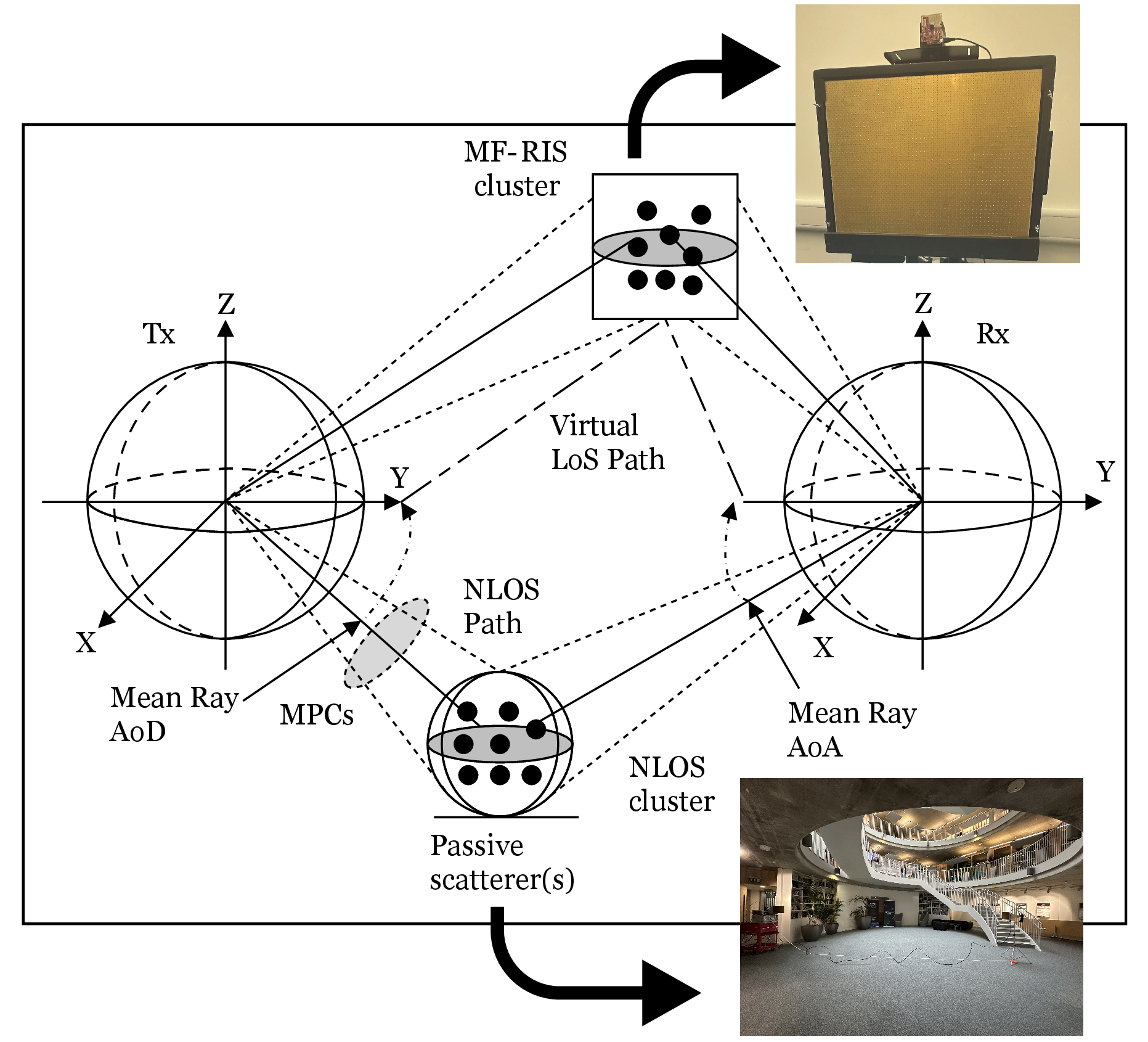
Figure 1: Overview of the GBSM applied to model the fast-fading channel (\(h_{\text{BS-RIS-UE}}\)) in this work..
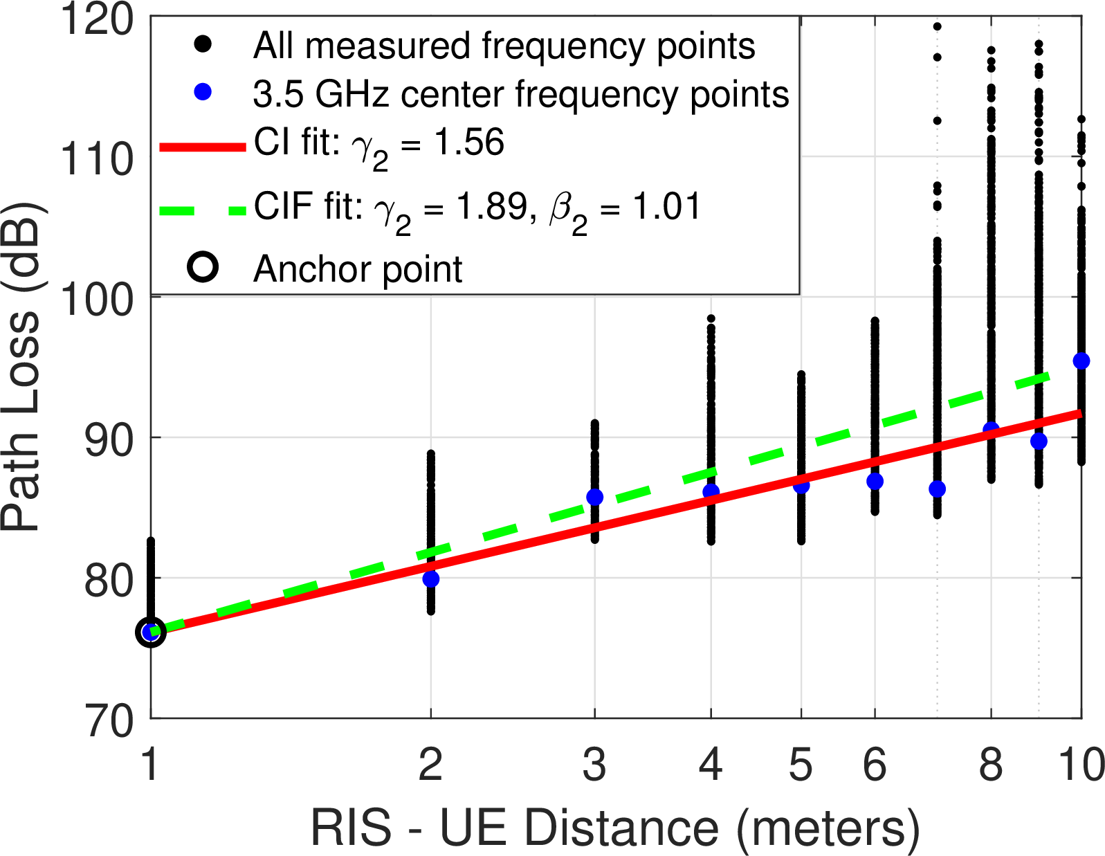
Figure 2: Measured \(h_{\text{BS-RIS-UE}}\) path loss exponent(s) based on the CI and the CIF model fits with variable \(d_{\text{RIS-UE}}\)..
3.2 Fast-Fading Channel Model↩︎
To accurately model fast-fading of the MF-RIS-assisted communication, we applied a GBSM model with multiple levels of randomness, which is illustrated in Fig. 1. This model fragments the indoor environment into \(Q\)-number of clusters, where all moving objects are typically assumed to be humans. Non-moving clusters are the static objects in the environment, such as walls, doors, or office furniture. A MF-RIS is also considered to be a static cluster, however, its response is reconfigured in several pre-defined ways according to its codebook, which is updated dynamically based on the moving cluster (assumed to be a UE) position. The resulting CIR is defined in terms of its large-scale (shadow fading, Ricean K-factor, delay spread, angular spreads) and small-scale (individual path delays, cluster powers, angles of arrival and departure, cross-polarization power ratios, per cluster shadowing) parameters. This model also considers a sustained linear motion, which is captured by assigning a mean Doppler shift to each moving cluster, where each cluster consists of \(I\)-number of rays. In idealized conditions with perfect reflections, each cluster would consist of exactly one ray, however, in practice, this number is a variable. If the scatterer represented by the cluster is rigid, the relative motion of the rays arises purely from the geometry and the motion of the cluster itself, and can be directly computed from the geometric model and known movement parameters. Additionally, there may be internal motion within a cluster, such as the motion of limbs, introducing further relative movement among rays. This intra-cluster motion can be modeled using a Doppler spectrum assigned to the cluster, however, ray-tracing estimation of intra-cluster parameters is known to be inaccurate and should be obtained from the measurement data instead [47].
We begin our analysis by expressing the high-level CIR of the BS-RIS-UE path in \((\tau,t)\)-domain: \[\begin{align} &h_{u,s,q,i}^{\text{BS-RIS-UE}}(\tau,t) = \\& \nonumber \left(h_{\text{BS-RIS}}\circledast h_{\text{RIS-UE}}\right)(\tau,t) + h_{\text{BS-UE}}(\tau,t), \label{eq:BS-RIS-UE} \end{align}\tag{4}\] where \(\circledast\) indicates convolution.
Assuming the plane wave incidence and that both the BS and the RIS are static, the CIR for each LoS path between the BS terminal \(s\) and the RIS can be adopted directly from the 3GPP TR 38.901 release 18.0.0 (7.5-29) [42]: \[\begin{align} \nonumber &h^{\text{BS-RIS}}_{s,1}(\tau,t) = \cdot\begin{bmatrix} F_{\text{RIS},\theta}(\theta_{\text{ZoA}}, \phi_{\text{AoA}}) \\ F_{\text{RIS},\phi}(\theta_{\text{ZoA}}, \phi_{\text{AoA}}) \end{bmatrix}^{T} \begin{bmatrix} 1 & 0 \\ 0 & -1 \end{bmatrix} \\[0.25em]& \nonumber \cdot \begin{bmatrix} F_{\text{BS},s,\theta}(\theta_{\text{ZoD}}, \phi_{\text{AoD}}) \\ F_{\text{BS},s,\phi}(\theta_{\text{ZoD}}, \phi_{\text{AoD}}) \end{bmatrix} \exp\left(-j 2\pi \frac{ d_{\text{BS-RIS}}}{\lambda_0}\right) \\[0.25em]& \cdot \exp\!\left(j 2\pi \frac{\hat{r}_{\text{BS},\text{LoS}}^{T} \vec{r}_{\text{BS},s}}{\lambda_0}\right) \delta\left(\tau - \tau_1^{\text{BS-RIS}}\right), \end{align}\] where \(F_{\text{RIS},\theta}\) and \(F_{\text{RIS},\phi}\) are the re-radiation patterns of the RIS in the direction of the spherical coordinates in a far-field \((\theta, \phi)\), \(F_{\text{BS},s,\theta}\) and \(F_{\text{BS},s,\phi}\) are the equivalent radiation patterns of the transmit antenna \(s\) in the direction of the spherical basis vectors \(\theta\) and \(\phi\) respectively, that both depend on the AoA, the AoD, the ZoA, and the ZoD, \(\hat{r}_{\text{BS}}^T\) is the spherical unit vector with azimuth departure angle for each BS antenna element, \(\lambda_0\) is the wavelength of a carrier signal, and \(\delta(\cdot)\) is the Dirac’s delta function. The measurement process of re-radiation patterns for the RIS used in this paper and its results are described in Section 6.4 of [45]. It is important to note that RIS re-radiation patterns change depending on the reflection angle, and should be either measured or simulated for each combination.
To express the CIR of the RIS-UE channel, we derived the double-bounce 3GPP-compatible SV model [48], which includes both the deterministic LoS component and the NLoS MPCs created by the RIS in the environment: \[\begin{align} \nonumber &h^{\text{RIS-UE}}_{1,u}(\tau,t) = \sqrt{\frac{K_R}{K_R+1}} \begin{bmatrix} F_{\text{UE},u,\theta}(\theta_{\text{ZoA}}, \phi_{\text{AoA}}) \\ F_{\text{UE},u,\phi}(\theta_{\text{ZoA}}, \phi_{\text{AoA}}) \end{bmatrix}^{T} \\[0.25em]& \nonumber \cdot\begin{bmatrix} 1 & 0 \\ 0 & -1 \end{bmatrix} \begin{bmatrix} F_{\text{RIS},\theta}(\theta_{\text{ZoD}}, \phi_{\text{AoD}}) \\ F_{\text{RIS},\phi}(\theta_{\text{ZoD}}, \phi_{\text{AoD}}) \end{bmatrix} \exp\left(-j 2\pi \frac{ d_{\text{RIS-UE}}}{\lambda_0}\right) \\[0.25em]& \cdot \exp\left( j 2\pi \frac{\hat{r}_{\text{UE},\text{LoS}}^T \vec{r}_{\text{UE},u}}{\lambda_0} \right) \exp\left( j 2\pi \frac{\hat{r}_{\text{UE},\text{LoS}}^T \vec{v}}{\lambda_0} t \right) \nonumber \\[0.25em]& \cdot \delta\left(\tau - \tau_1^{\text{RIS-UE}}\right) \nonumber\\[0.25em]& + \sqrt{\frac{1}{K_R+1}} \sum_{q=1}^Q\sum_{i=1}^{I_q}\sqrt{\frac{P_q}{I_q}} \begin{bmatrix} F_{\text{UE},u,\theta}(\theta_{q,i,\text{ZoA}}, \phi_{q,i,\text{AoA}}) \\ F_{\text{UE},u,\phi}(\theta_{q,i,\text{ZoA}}, \phi_{q,i,\text{AoA}}) \end{bmatrix}^{T} \nonumber \\[0.25em] &\cdot \begin{bmatrix} \exp(j \Phi_{q,i}^{\theta\theta}) & \sqrt{\kappa_{q,i}^{-1}} \exp(j \Phi_{q,i}^{\theta\phi}) \\ \sqrt{\kappa_{q,i}^{-1}} \exp(j \Phi_{q,i}^{\phi\theta}) & \exp(j \Phi_{q,i}^{\phi\phi}) \end{bmatrix} \nonumber \\[0.25em]& \cdot \begin{bmatrix} F_{\text{RIS},\theta}(\theta_{\text{q,i,ZoD}}, \phi_{\text{q,i,AoD}}) \\ F_{\text{RIS},\phi}(\theta_{\text{q,i,ZoD}}, \phi_{\text{q,i,AoD}}) \end{bmatrix} \exp\left( j 2\pi \frac{\hat{r}_{\text{UE},q,i}^T \vec{r}_{\text{UE},u}}{\lambda_0} \right) \nonumber \\[0.25em]& \cdot \exp\left( j 2\pi \frac{\hat{r}_{\text{UE},\text{q,i}}^T \vec{v}}{\lambda_0} t \right) \delta\left(\tau - \tau_{q}^{\text{RIS-UE}} -\tau_{q,i}^{\text{RIS-UE}}\right), \label{eq:ris-ue} \end{align}\tag{5}\] where \(K_R\) is the Ricean K-factor in \(\text{dB}\) which refers to a power ratio between the deterministic component and the stochastic components (i.e. the main reflected path and other MPCs), \(Q\) is the number of clusters, \(I_q\) is the number of rays per cluster, \(\hat{r}_{\text{UE}}^T\) is the spherical unit vector with azimuth departure angle for each UE antenna element, \(\phi_{\text{AoD}}\) and elevation departure angle \(\theta_{\text{ZoD}}\), \(\vec{r}_{\text{UE},u}\) is the location vector of receive antenna at the UE, \(\vec{v}\) is the velocity vector of the UE with speed \(v\) and travel direction angles \(\left(\phi_v,\theta_v\right)\), \(\Phi_{q,i}^{\theta\phi}\) denote random initial phases for path \(i\) in cluster \(q\) for four different polarization combinations in CIRs, and \(k\) is the XPR for each ray \(i\) of each cluster \(q\), such that: \[k_{q,i} = 10^{X_{q,i}/10},\] where \(X_{q,i} \sim N \left(\mu_{\text{XPR}},\sigma_{\text{XPR}}\right)\) is Gaussian (i.e. normal) distributed with \(\mu_{\text{XPR}}\), and \(\sigma_{\text{XPR}}\) values given in Table 7.5-6 of [42], and \(P_q\) are the cluster powers defined as: \[P_q= \frac{P^\prime_q}{\sum^Q_{q=1}P^\prime_q},\] \[P^\prime_q = \exp{\left( -\tau_q \frac{\omega_\tau-1}{\omega_\tau DS} \right)\cdot10^{\frac{-Z_n}{10}}},\] where \(DS\) is the delay spread, \(\omega_\tau\) is the decay rate, and \(Z_{n} \sim N (0,\zeta^2)\) is the per-cluster shadowing term in \(\text{dB}\), which depends on the delay distribution.
None
Figure 3: No caption.
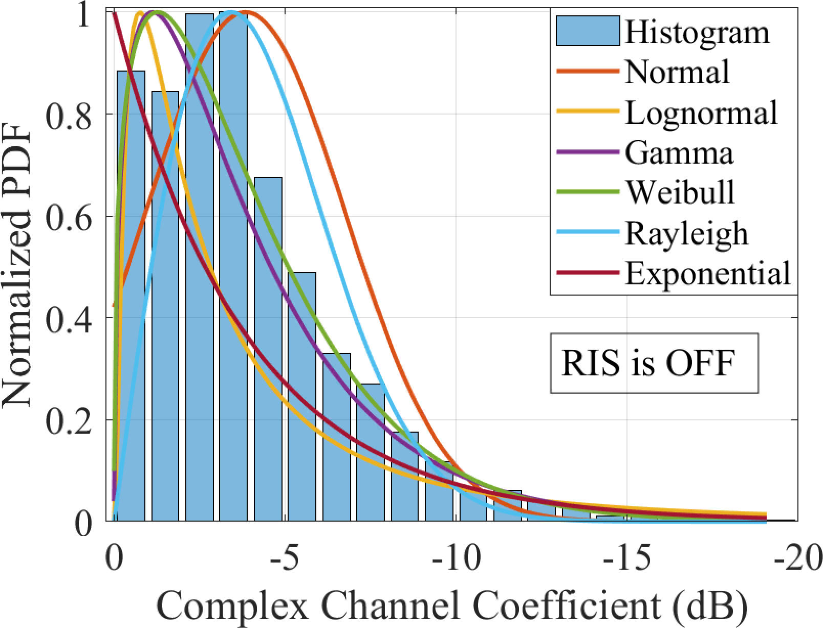
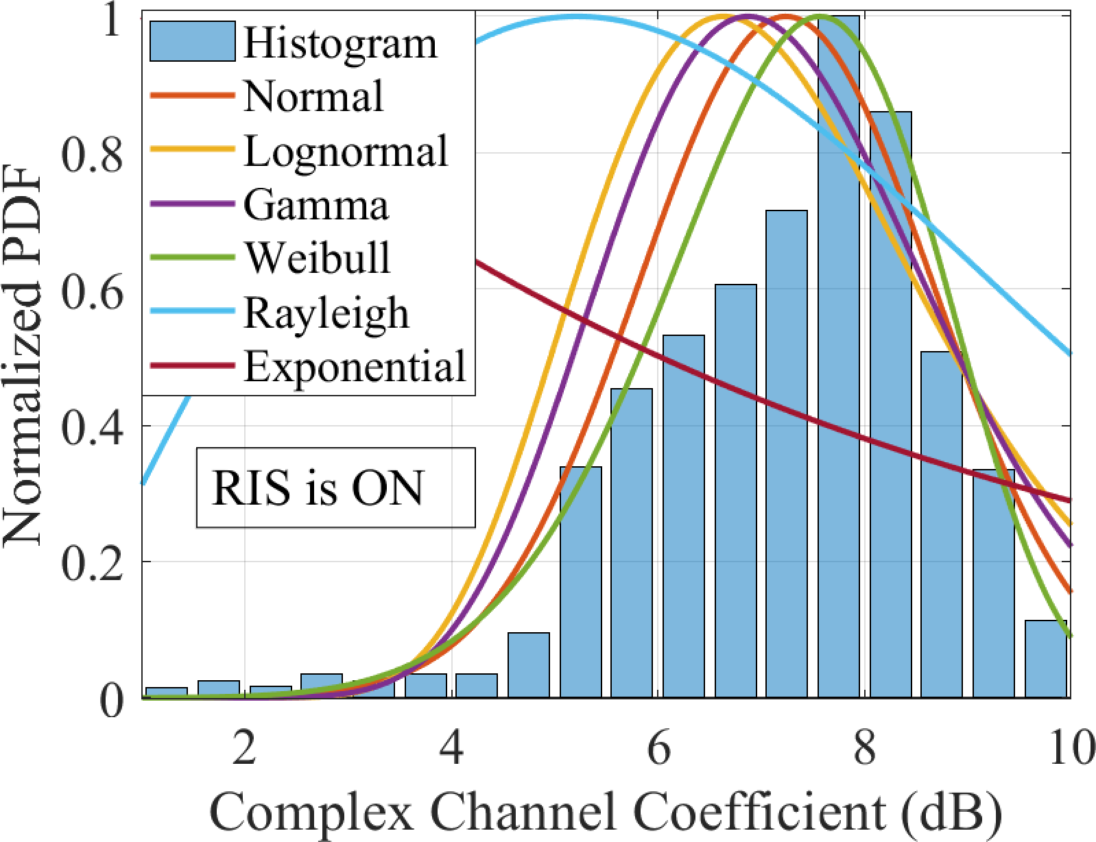
Figure 4: Channel histograms for the UE coordinate (40\(^\circ\), 90\(^\circ\), 2m) plotted on measured PDP with: a) RIS switched OFF, showing fading in the BS-UE NLoS channel, and b) RIS switched ON, showing fading in the cascaded BS-RIS-UE channel i.e. the vLoS..
Our measurements confirm that the effects of the NLoS \(h_{\text{BS-UE}}\) channel should not be ignored, as the NLoS component from the BS is inevitably present at the UE due to MPCs and scattering in the environment with \(O\)-number of clusters and \(W_o\)-number of rays in these clusters, that may be different from the rays and clusters in the RIS-UE path. This is especially evident in the Sub-6 GHz indoor channel when \(h_{\text{BS-RIS}}\) and \(h_{\text{RIS-UE}}\) are both LoS paths, thereby creating the vLoS with the RIS. Therefore, we also consider the CIR of the NLoS \(h_{\text{BS-UE}}\) path, derived in 3GPP TR 38 901 (7.5-22) [42]. Then, equation (5 ) can be expanded to describe the CIR of the cascaded \(h_\text{BS-RIS-UE}\) channel as the finalized expression in (3). Note that the basis-reconciliation sign flip \(\left(\text{diag}\left(1,-1\right)\right)\) cancels out, as it is applied on both sides of the RIS re-radiation patterns, and the RIS is assumed to be a scalar (i.e., diagonal). Also note that this formulation assumes that the \(h_\text{BS-RIS}\) channel is a LoS, the \(h_\text{BS-UE}\) channel is NLoS (i.e. scattered), and neither the BS nor the RIS is moving.
The derived CIR is compatible with the 3GPP-developed framework for ISAC, and can be used in channel estimation and wireless ray-tracing simulation platforms, such as the ones described in [49]–[51]. The resulting channel can be visualized with a PDF of the measured \(h_{\text{BS-RIS-UE}}\), as shown in Fig. 4 (b), with the UE coordinate \((\theta,\phi,d) = (40^\circ, 90^\circ, 2\text{m})\), and compared with a no-RIS scenario in Fig. 4 (a). The PDF significantly differs from the conventional Rayleigh distribution with the RIS. Instead, the channel distribution is most closely matched to the Weibull distribution in this case, but the log-normal distribution is the most fitting when the bandwidth is reduced to 200 MHz.
4 MF-RIS-enabled RCC system↩︎
Through the combination of the analysis shown in Sections 2 and 3, this section provides the analysis of the complex MF-RIS system with decoupled RCC tasks.
4.1 MF-RIS Algorithm for Localization of a Moving User↩︎
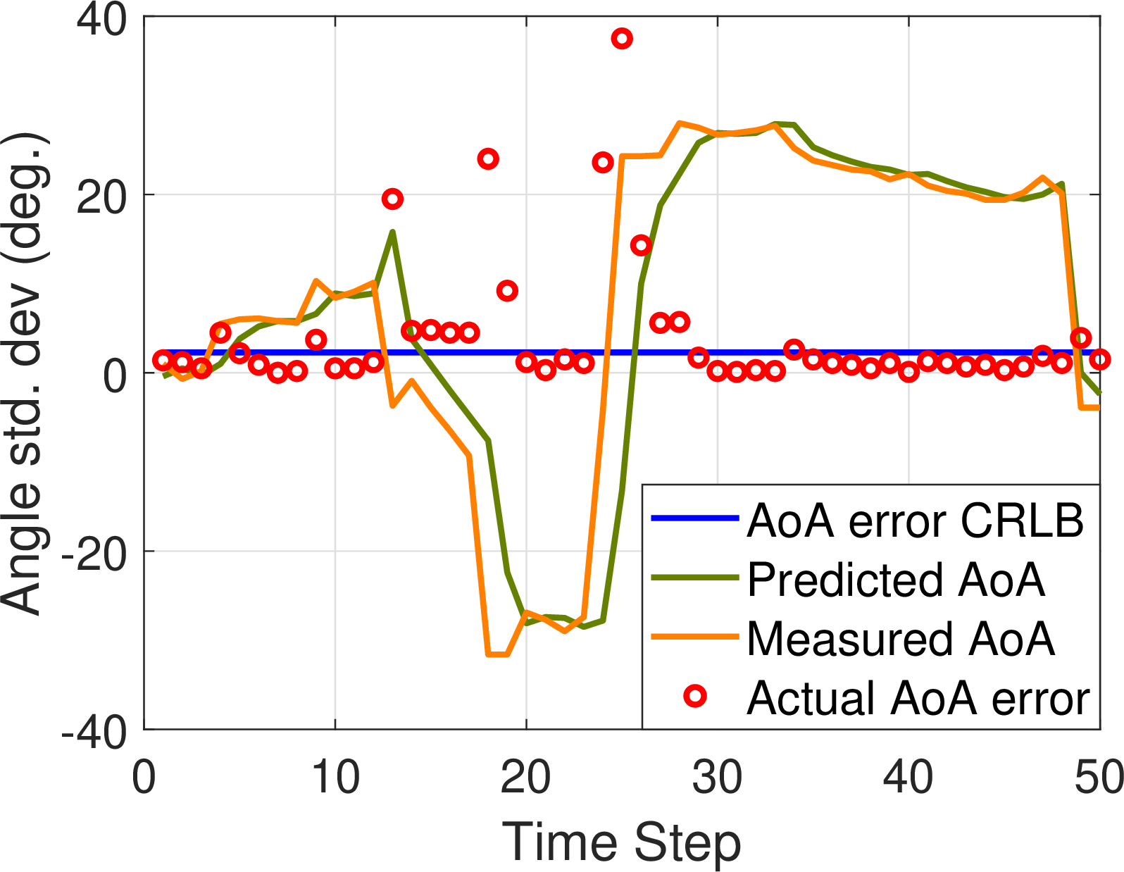
Figure 5: Horizontal AoA Tracking: CRLB vs predicted AoA vs measured AoA from a UE moving in the radar’s FoV, and the resulting AoA error..
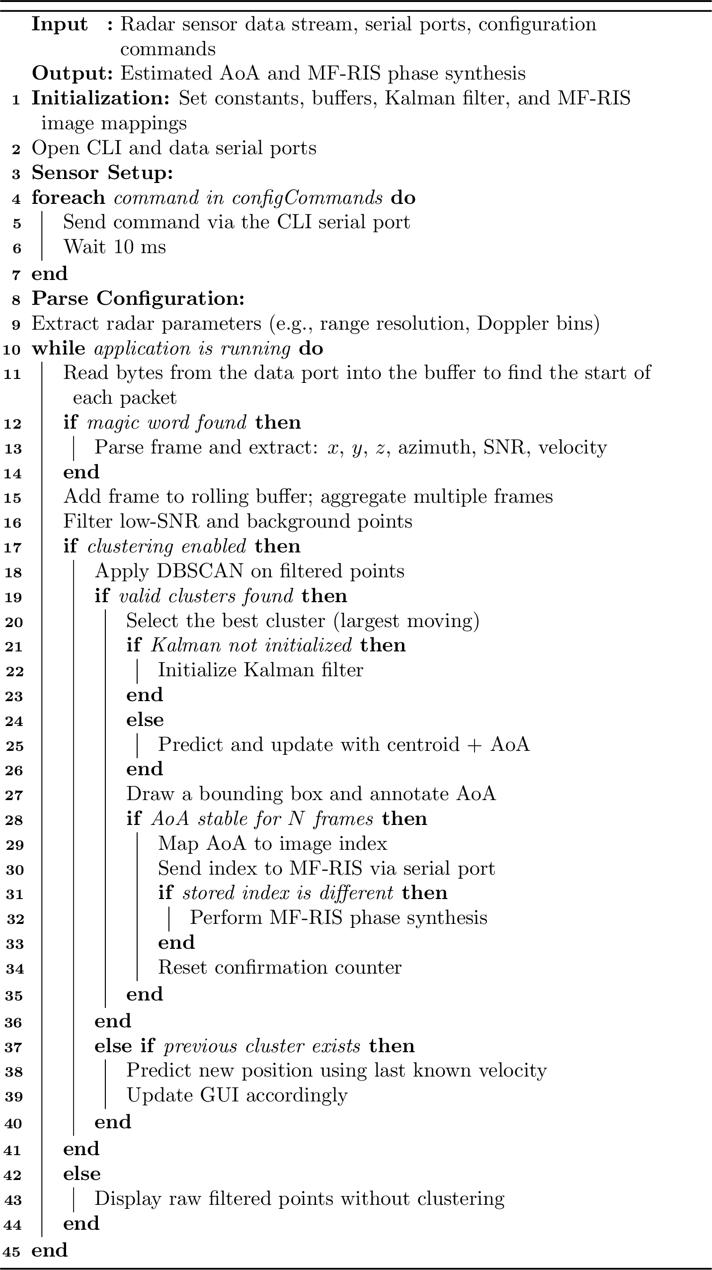
The Kalman filter prediction can be implemented on each separate term of the UE position coordinate \(\left(\theta^\prime_k, \phi^\prime_k,r^\prime_k\right)\) detected by the mmWave radar. To illustrate, in Fig. 5, the CRLB of the theoretical minimum AoA error is plotted for the mmWave radar, previously derived in [52], and compared against the predicted Kalman filter output \((\theta^\prime_k)\), as well as the measured horizontal AoA \((\theta_k)\), therefore showing the actual AoA estimation error with red circles. This measurement was obtained with the user moving within the FoV of the radar at a 2 m distance. The mmWave radar hardware is based on the TI IWR6843ISK 60 GHz MIMO radar development kit with 3 TX antennas, 4 RX antennas, transmit power \(12~ \textrm{dBm}\), and \(\mathrm{10~MHz}\) IF bandwidth. As can be seen from the figure, a sudden movement or a trajectory change of the UE can introduce a significant AoA error, however, the Kalman filter prediction error is greatly reduced within 3-4 frame durations, after which the AoA error becomes aligned with the CRLB, while the UE is static or moving with a constant velocity. Note that the frame duration (i.e. prediction latency) depends on the SBC speed and loading of the MCU. The average prediction latency 127 ms was measured over one minute with the MF-RIS ranging between 27 ms (fastest timestamp) and 297 ms (slowest timestamp) with the average horizontal AoA \((\theta_k)\) error 6.47\(^\circ\). This result is deemed appropriate for an indoor-centric setup. However, in an outdoor-centric setup such performance might be sub-optimal, therefore requiring more sophisticated hardware. The developed MF-RIS phase update algorithm is summarized in Algorithm 6.
4.2 MF-RIS-Induced Channel Hardening Effect↩︎
The instantaneous SNR of the system in (3) is derived as: \[\text{SNR} = \frac{P^{\text{Tx}}_{s}}{\eta^2}\left(\sum^L_{l=1} \left|h_{u,s}^{\text{BS-RIS-UE}}(\tau,t)\right|\right)^2, \label{eq:SNR}\tag{6}\] where \(P^{\text{Tx}}_{s}\) is the transmit power, \(\eta\) is the noise variance, and \(L\) defines the number of channels. It follows from (6 ) that randomness in \(h_{\text{BS-RIS}}\), \(h_{\text{RIS-UE}}\), and \(h_{\text{BS-UE}}\) causes SNR fluctuations, degrading communication performance. When these variations average out, the channel exhibits hardening [53]–[55], meaning the random SNR can be approximated by a deterministic term. Practically, this implies \(\text{SNR} \approx L^2\) times a constant for large \(L\), where \(\left(h_{\text{BS-RIS}},h_{\text{RIS-UE}},h_{\text{BS-UE}}:l=1,...,L\right)\) are random sequences converging to deterministic values. Therefore, channel hardening occurs when \(h_{\text{BS-RIS-UE}}\) dominates over \(h_{\text{BS-UE}}\).
Just as random channel gains cause SNR fluctuations, random multipath delays cause fluctuations in the instantaneous coherence bandwidth \(B_c(t)\), as outlined in Chapter 4.5 of [56] with several practical examples. To summarize, in NLoS with many reflections, the RMS delay spread \(\tau_{\text{RMS}}\) is large, giving a small \(B_c(t)\) and strong frequency selectivity. However, in RIS-enabled vLoS with small delay spread, \(B_c\) is large instead, giving near flat fading. With mobility and path geometry changes, delay spread alters and thus \(B_c(t) \approx 1/5 \times \tau_{\text{RMS}}(t)\), which is an estimate that assumes that the frequency correlation between subcarriers is equal to 0.5 (i.e., moderately similar channel gains/phases). Hence, just as (6 ) shows power fluctuations from random gains, \(B_c(t)\) captures frequency-domain variability, explaining unstable throughput in mobile NLoS 5G NR channels.
To reduce the frequency selectivity of the channel, we propose to minimize the delay spread \(\tau_{\text{RMS}}\) by maximizing \(B_c\) through real-time MF-RIS system configuration. We can formulate the corresponding optimization problem in terms of the set of phase shifts \(\left(\Psi_{m,n}\right)\) on MF-RIS. Similar to sum-rate maximization, the problem can be written as an arg-minimization of the RMS delay spread: \[\begin{align} & \mathbf{\Psi_{m,n}^{\star}} = \underset{{\Psi_{m,n}}}{\arg\min} \;\tau_{\text{RMS}}(t), \\& \nonumber \text{s.t.} \;\Psi_{m,n} \in [0^\circ, 360^\circ], \quad \forall m,n. \end{align}\]
Equivalently, this optimization problem can be written as the maximization of the coherence bandwidth: \[\begin{align} \mathbf{\Psi_{m,n}^{\star}} = \underset{{\Psi_{m,n}}}{\arg\max}\;B_c(t) = \underset{{\Psi_{m,n}}}{\arg\max} \;\frac{1}{5~\tau_{\text{RMS}}}{(t)}~, \end{align}\] In other words, by dynamically adjusting phase shifts on the MF-RIS, the channel’s delay spread is compressed and the channel appears flat over a larger bandwidth for a given UE, thus preventing throughput fluctuations when it is moving.
From this analysis, it can be observed that the optimization of both SNR and the coherence bandwidth for MF-RIS-assisted communication can cause a slight trade-off under specific circumstances. For example, if there are multiple paths (e.g., a direct LoS path and a MF-RIS-created vLoS path with a longer delay), maximizing SNR might involve constructively adding both – but that introduces a larger delay gap between them. Minimizing delay spread might instead favor one dominant path and suppress secondary paths. Then, the codebook design might sacrifice some power from a late-arriving path to keep the channel more time-concentrated. Therefore, there is a balance between power maximization and delay alignment. In this work, we focus on the latter and use the standard deviation of channel throughput as the performance metric for evaluating the MF-RIS-induced channel hardening effect.
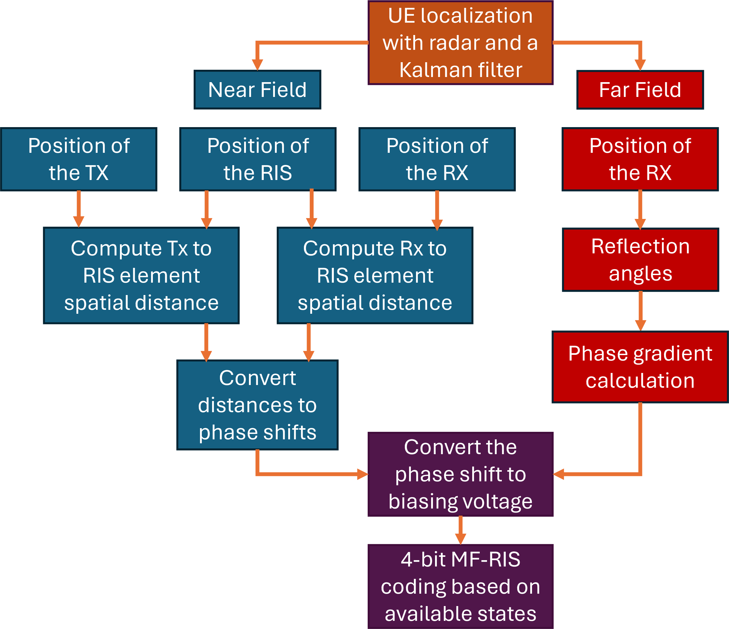
Figure 7: MF-RIS phase synthesis algorithm for near-field and far-field domains..
5 MF-RIS Phase Synthesis for Near-Field and Far-Field Domains↩︎
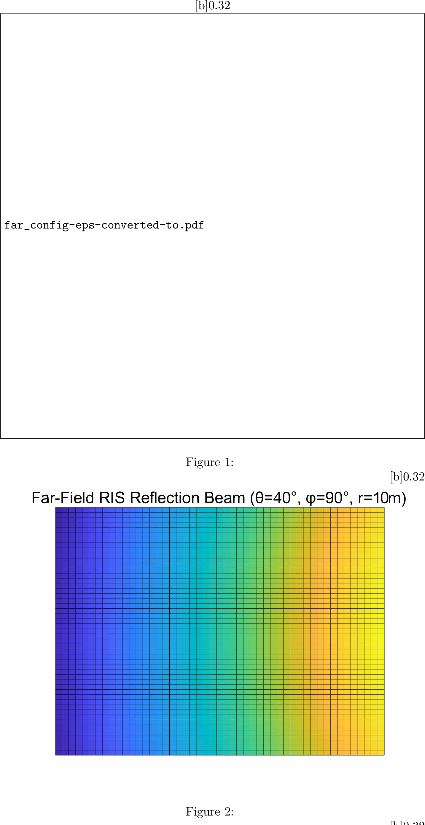
The propagation characteristics of the RIS-assisted channel depend on EM interactions between the incident, reflected, and scattered waves. In an idealized far-field scenario, the RIS reflection follows a planar wavefront-based uniform phase gradient model, while near-field scenarios require more complex modeling. Specifically, the near-field focusing effect is influenced by spherical wavefront models and evanescent waves, which decay exponentially beyond the RIS surface but contribute significantly to subwavelength focusing. Thus, configurations should use spatially dependent formulations rather than only angular steering. Accurate modeling across both domains requires careful modeling of wave propagation and scattering. At \(3.5~\text{GHz}\), corresponding to a wavelength of approximately \(0.0857~\text{m}\), the behavior of the RIS changes significantly as the measurement distance shifts from the near-field at 2 m to the far-field at 10 m. Therefore, we propose and illustrate the MF-RIS phase synthesis algorithm in Fig. 7, showing that the codebook generation process differs fundamentally between the far-field and near-field domains.
5.1 Near-Field Codebook↩︎
When the transmitter or receiver lies within the Fraunhofer distance \(<2D^2/\lambda\) (with \(D\) the largest RIS dimension), the impinging and reflected wavefronts must be modeled as spherical rather than plane waves to maximize the RIS beamforming gain. This relationship is conventionally modeled through the Green’s function–based 3D coupling among the BS, the RIS elements \((m,n)\), and the UE, as shown below: \[\mathbf{E}(\mathbf{r}) \;=\; \sum_{m=1}^{M}\sum_{n=1}^{N} \Gamma_{m,n}\, \frac{e^{-j k \big(\|\mathbf{r}_{m,n}^{\text{BS--RIS}}\|+\|\mathbf{r}_{m,n}^{\text{RIS--UE}}\|\big)}}{\|\mathbf{r}_{m,n}^{\text{BS--RIS}}\|\,\|\mathbf{r}_{m,n}^{\text{RIS--UE}}\|}, \quad k=\tfrac{2\pi}{\lambda}, \label{eq:GF}\tag{7}\] where \(\Gamma_{m,n}\) is the (generally complex) reflection coefficient of the \((m,n)\)-th RIS element, \(\mathbf{r}_{m,n}^{\text{BS--RIS}}\) and \(\mathbf{r}_{m,n}^{\text{RIS--UE}}\) are the BS–to–element and element–to–UE distance vectors, respectively, \(\lambda\) is the wavelength, and \(\|\cdot\|\) denotes the Euclidean norm.
By appropriately adjusting \(\Gamma_{m,n}\), the superposition of the scattered fields can be engineered to focus within the near-field region. Let \(\Psi_{m,n}\) denote the programmed phase of the \((m,n)\)-th unit cell. To ensure that all contributions in 7 add in phase at the focal point, the RIS should compensate both the propagation phase and the residual quadratic (Fresnel) curvature from the two hops. In other words, the phase delays due to propagation from BS to \((n,m)\) and from \((n,m)\) to UE should be exactly compensated by the MF-RIS element’s added phase and the MF-RIS focal point: \[\begin{align} &\Psi_{m,n}^{\text{NF}} = \operatorname{mod}\!\Bigg\{ -k\!\left(\big\|\mathbf{r}_{m,n}^{\text{BS--RIS}}\big\| +\big\|\mathbf{r}_{m,n}^{\text{RIS--UE}}\big\|\right) \nonumber\\ &\;\;-\;\frac{k}{2}\,\big(x_{m,n}^2+y_{m,n}^2\big)\! \left( \frac{\cos^{2}\theta_{i}}{\big\|\mathbf{r}_{m,n}^{\text{BS--RIS}}\big\|} +\frac{\cos^{2}\theta_{r}}{\big\|\mathbf{r}_{m,n}^{\text{RIS--UE}}\big\|} \right) \;,\; 2\pi \Bigg\}, \label{eq:NF} \end{align}\tag{8}\] where \(x_{m,n}\) and \(y_{m,n}\) are the 2D coordinates of the \((m,n)\)’th RIS element, and \(\theta_{i}\) and \(\theta_{r}\) are the incidence and reflection angles (with respect to the RIS normal). Note that the conversion from spherical to Cartesian coordinates is required to realize the reflection in the desired reflection angle \(\left(\theta_r, \phi_r\right)\).
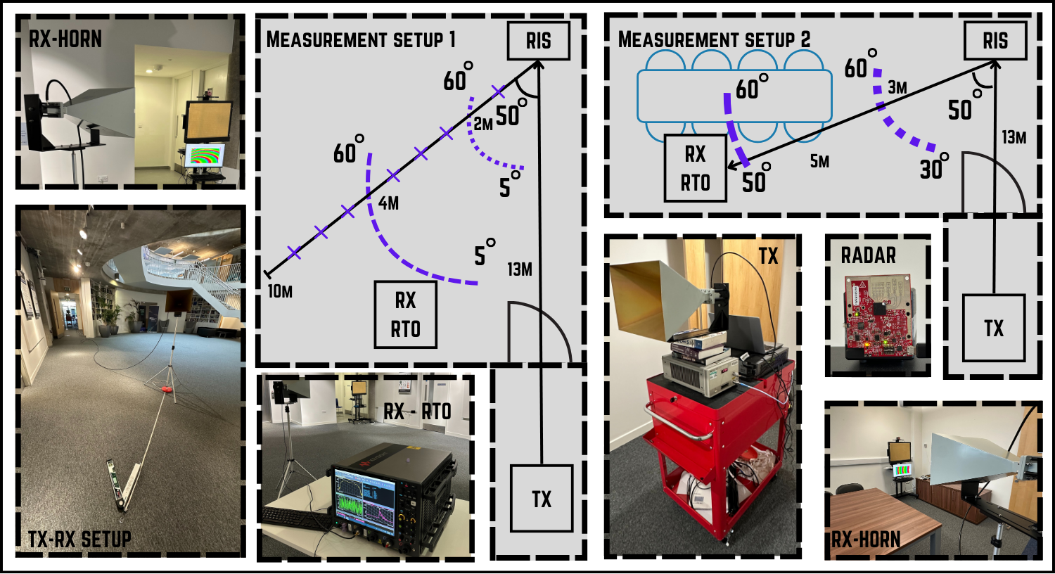
Figure 10: Static measurement setup: RIS reflecting the signal from a TX located in a far-field towards a RX located at varied distances in \(5^\circ\) angle and 1 m steps. A large indoor space and a small meeting room were evaluated..
5.2 Far-Field Codebook↩︎
As the UE moves further away from MF-RIS, such as to 10 meters or beyond, the spherical curvature of the wavefronts diminishes and the far-field assumption becomes valid, making the contributions from distance-based terms negligible. In this case, a linear phase gradient suffices for RIS beamsteering: \[\begin{align} \Psi_{m,n}^{\text{FF}} = & \operatorname{mod}\Bigg\{ -k \Big( x_{m,n}\,\sin\theta_r \cos\phi_r \\ & + y_{m,n}\,\sin\theta_r \sin\phi_r \Big),\, 2\pi \Bigg\}, \notag \end{align}\] This model assumes a planar incident wavefront with \(\left(\theta_i,\phi_i\right) = (0^\circ,0^\circ)\) and a uniform array structure.
To illustrate these principles, Fig. 8 shows the RIS configuration for \(\theta=40^\circ\), \(\phi=90^\circ\) at 2 meters, the RIS near-field beam pattern, and the corresponding peak of the PDP for RIS on and off cases. Fig. 9 presents the same comparison using a linear phase gradient codebook in the far-field regime at 10 meters. PDP peak shows 17.5 dB \(/\) 7.5 dB improvement with RIS in the near-field and the far-field, respectively.
| Operating Frequency | 3.5 GHz (centre) |
|---|---|
| Bandwidth | 800 MHz |
| Type | Reflective |
| Polarization | Dual-polarized |
| Size | 570 mm \(\times\) 420 mm |
| Number of unit cells | 50 \(\times\) 37 with \(\lambda/8\) spacing (1,850 in total) |
| Unit cell control | 4-bit digital |
| Switching element | Varactor diode |
| Power consumption | 2.2 W (RIS) + 2 W (Radar) + 10 W (SBC) |
6 Channel Measurement Setup↩︎
All measurements were performed in the ICS, 5G / 6G Innovation Centre, University of Surrey. Measurement setups used in this paper are shown in Fig. 10 and consider two of the typical indoor RIS use-case scenarios: a) a large auditorium hall \(\left(14.6\times10.8~\mathrm{m}^2\right)\), and b) a meeting room \(\left(7.3\times4.3~\mathrm{m}^2\right)\). In either case, the LoS path between the BS and the UE is blocked, however, the NLoS path exists, which was confirmed with measurement.
6.1 Device Under Test↩︎
All measurements were carried out using the SMV2201-040LF varactor diode-based 4-bit RIS, which has a centre frequency of 3.5 GHz and the other characteristics listed in Table ¿tbl:table95RIS95spec?. It utilizes matrix-based control of 1,850 unit cell elements, arranged in 37 rows and 50 columns, resulting in a total aperture size of 420 x 570 mm. This RIS forms a part of the MF-RIS system with sensing capabilities, where the 60 GHz mmWave radar IWR6843ISK by TI is used for implementing the custom UE tracking algorithm on the Seedstudio ODYSSEY X86J4125800 SBC to dynamically update the MF-RIS codebook.
6.2 Static Measurement↩︎
In this setup, the RX remained static, and the measurements were taken from designated positions rather than in real-time. The transmitted signals were generated using a Keysight M8195A waveform generator at the TX, amplified by a 21 dBm gain LNA. At the RX, a Keysight UXR0334B Infiniium RTO captured the resulting complex channel responses. Both the TX and RX employed identical A-INFOMW LB-229-20-C-SF horn antennas, each providing 20 dBi gain. A total of 1024 symbols were transmitted at a rate of 800 Msps, corresponding to a FFT length of 1024 and an operational bandwidth of 800 MHz, giving a delay bin resolution of 1.25 ns and a corresponding distance resolution of 0.375 m. The RTO was calibrated at the cable ends to remove connector losses and non-linearities of the LNA. Each measurement was repeated three times to ensure repeatability. The measurements were used to obtain the time-domain channel response, with each response averaged over 50 individual realizations. From these responses, the PDP and RMS delay spread were derived at each measurement point to characterize the static propagation environment and MPCs. Both the transmitting antenna and the receiving antenna were positioned at a height of 1.45 m above the floor, aligning them with the centre of the RIS. The position of TX and RIS was fixed, whereas the position of the RX was adjusted between near-field (2 m) and far-field (10 m) distances for different measurements. Measurements were taken at angles between 5\(^\circ\) to 60\(^\circ\) every 5\(^\circ\) steps for further verification of the RISs performance. The orientation of the RX relative to the RIS was configured to suit the reflection profile of the RIS. During the measurements, there was no human presence or moving objects, ensuring that the channel remains time-invariant. Data from each measurement session was recorded on the RTO, subsequently transferred, and analyzed using MATLAB.
6.3 Dynamic Measurement↩︎
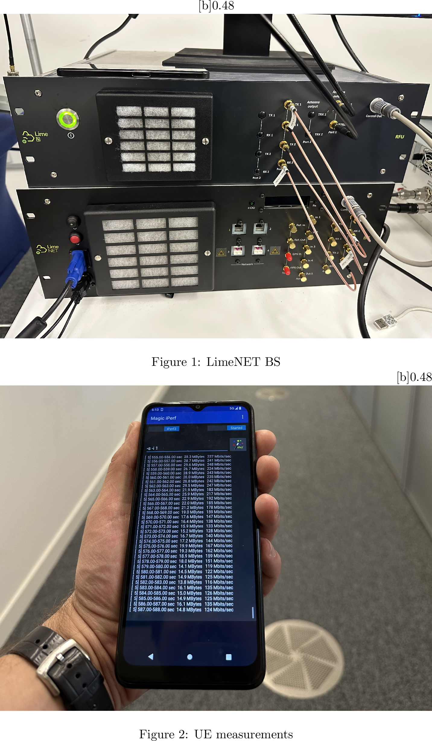
To perform the channel measurement of a dynamically moving UE, the LimeNET 5G NR 2x2 MIMO system shown in Fig. 11 was used in a single user configuration. The system produces a 3.5 GHz modulated waveform with an initial power of 10 dBm and 30 dBm connected to two A-INFOMW LB-229-20-C-SF standard 20 dBi gain horn antennas, both aiming the wavefront towards the MF-RIS. On the receiving side, the 4x4 MIMO smartphone was wirelessly attached to the LimeNET network and equipped with iPerf software to monitor the channel quality characteristics. The smartphone position was moved dynamically within the MF-RIS near-field at 2 m and 4 m distances across 5-60\(^\circ\) angular range with a constant velocity, while observing throughput as a system evaluation metric.
7 Results and Analysis↩︎
This section presents the results obtained from the empirical data collected from the measurement. Large-scale and small-scale channel parameters are summarized in Tables III and IV, which were obtained from the two static measurement setups described previously. Note that clustering distributions are based on normalized PDP, and absolute values should be obtained by applying the path loss that was obtained at the center frequency corresponding to the PDP peak. At the end of the section, the dynamic UE throughput measurement results on the LimeNET MIMO system are described and illustrated in Fig. 13. Note that the calculated theoretical maximum throughput for this 2\(\times\)2 MIMO system is 571.1 Mbps.
4pt
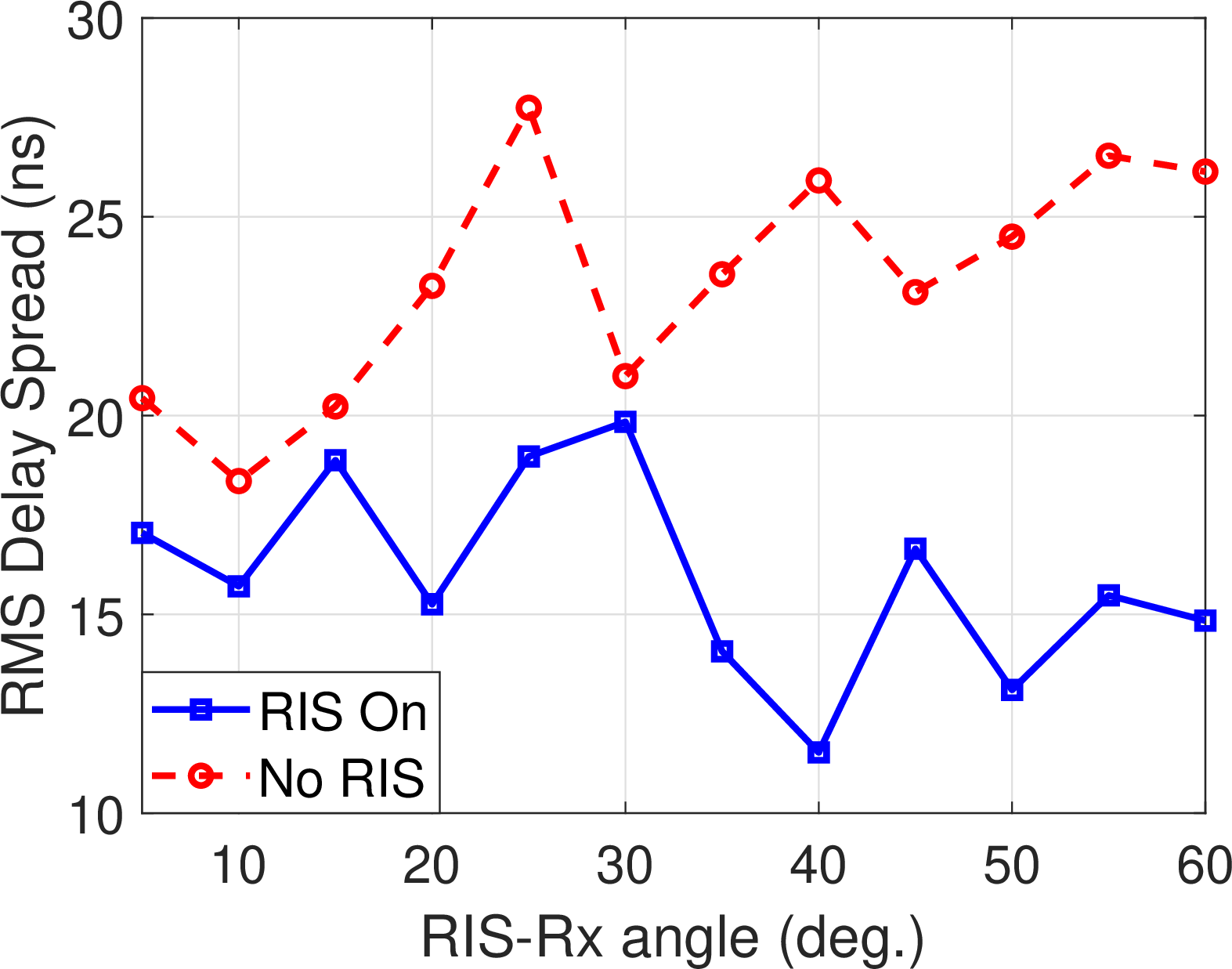
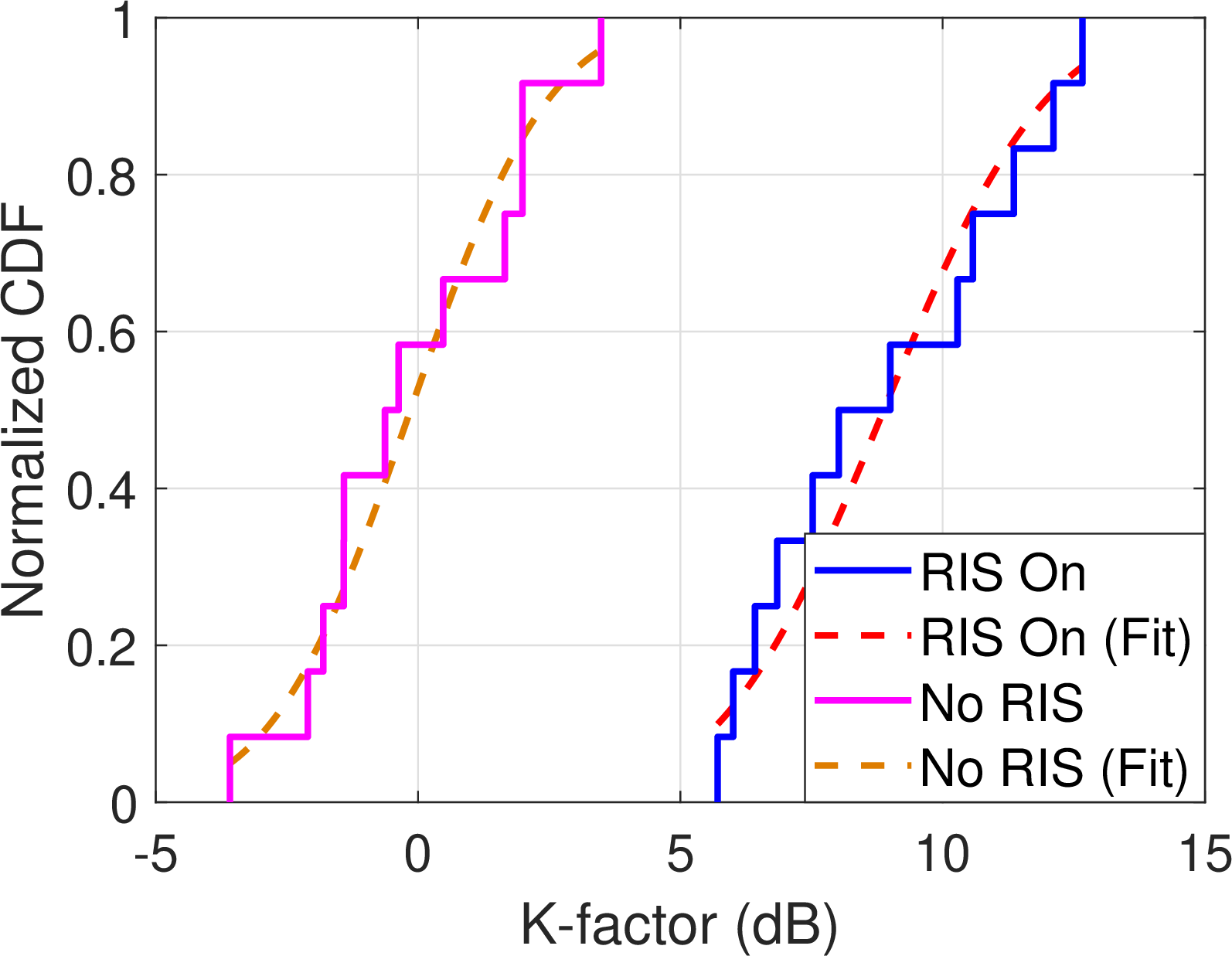
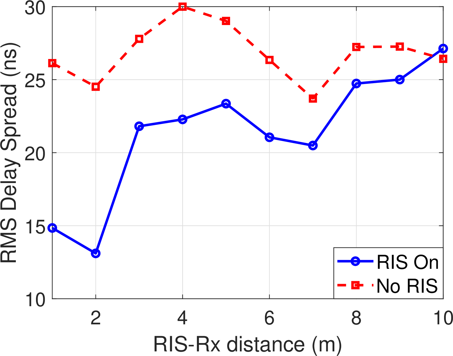
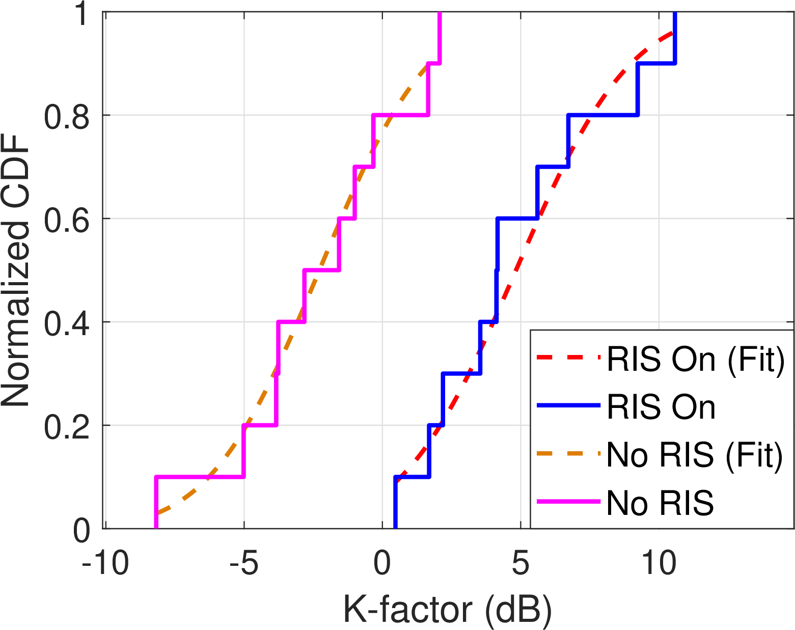
Figure 12: RMS delay spread and K-factor analysis of raw PDPs: 1. Angular measurements between 5\(^\circ\)-60\(^\circ\) at a fixed RIS-Rx distance of 2m: a) RMS delay spread, b) CDF of the K-factor and the normal fit. 2. Spatial measurements for RIS-Rx distances between 1-10m with fixed 50\(^\circ\) reflection angle: c) RMS delay spread, d) CDF of the K-factor and the normal fit..
7.1 Delay Spread and K-factor Analysis↩︎
The performance of the RIS in the static setup is largely assessed through RMS delay spread and K-factor analysis across angles and distances, as shown in Fig. 12. For angular measurements, the delay spread increases at wider angles without RIS, as the Rx becomes more exposed to MPCs coming from the wall located behind the RIS. With the RIS on, the delay spread decreases and the vLoS peak dominates, concentrating energy around the main component (i.e., hardening the channel). For distance measurements, the RIS on case shows an increasing delay spread with Rx separation due to added MPCs from surrounding scatterers, which highlights that the channel hardening effect of the RIS drops as the Rx is moved from near-field to far-field. Without the RIS, the channel fluctuates without a clear trend, as expected. The K-factor results confirm these trends. The angular sweep without RIS shows a narrower distribution around low values (–3.5 dB to 3.5 dB), while the RIS on case yields higher values (5.5 dB to 13 dB) due to the stronger LoS. The distance sweep shows that the K-factor decreases with RIS-Rx separation as the vLoS weakens and multipath grows, consistent with the rising delay spread. In contrast, without the RIS, the K-factor remains low and scattered (–7 dB to 2.5 dB).
Clustering analysis also shows that the number of significant delay taps and overall delay spread increase with distance and at wider angles, highlighting how the addition of RIS not only creates the vLoS but also alters the structure of the multipath environment.
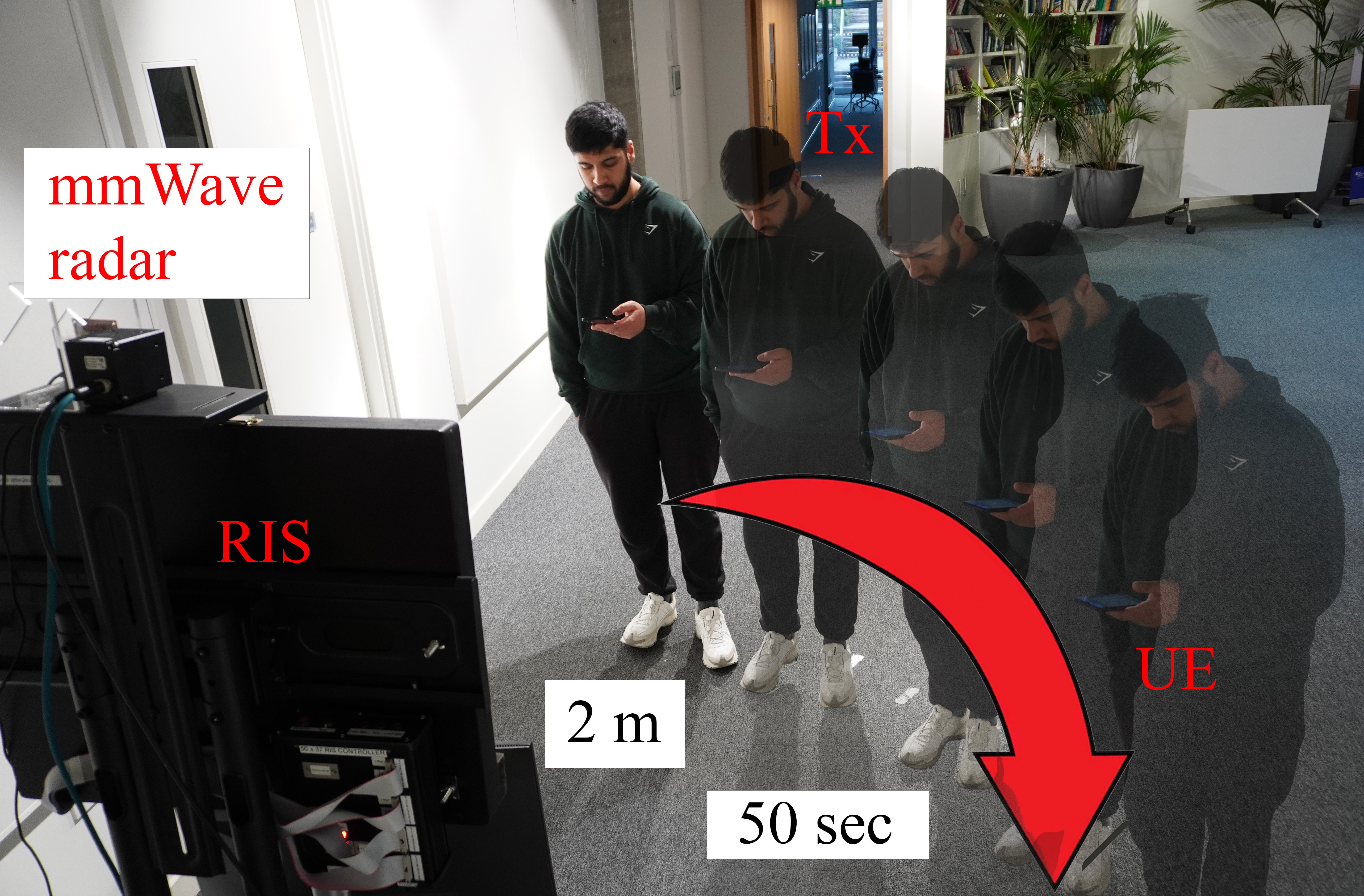
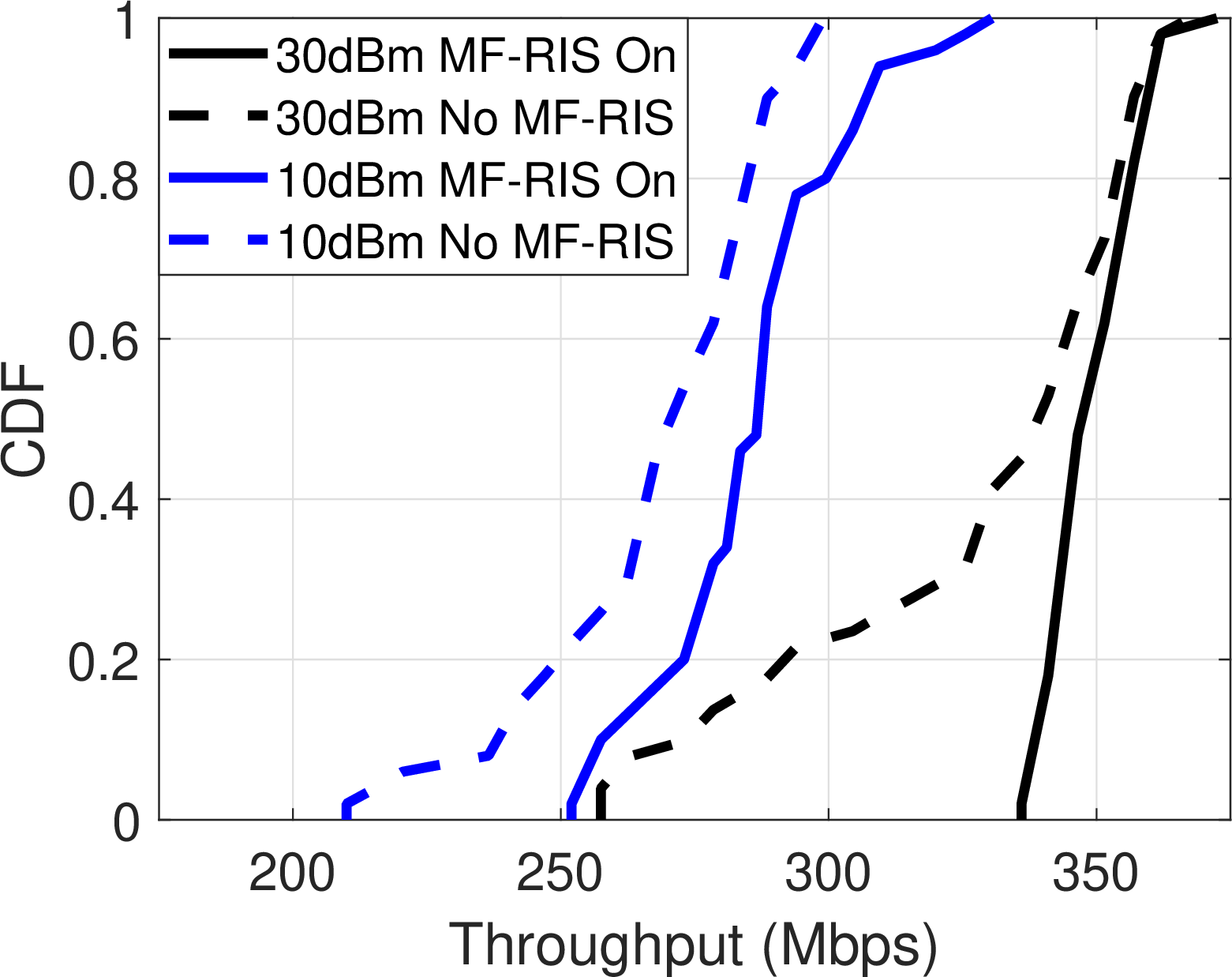
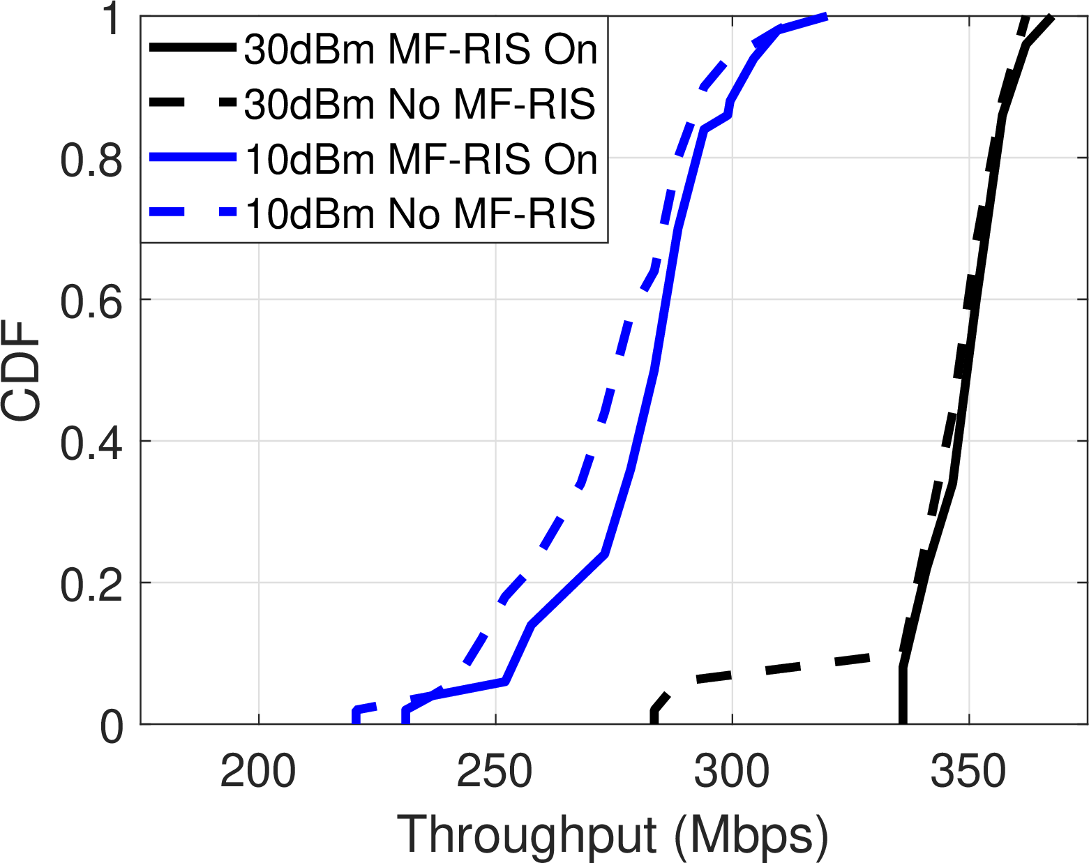
Figure 13: System throughput measurements in the near-field: a) MF-RIS-enabled RCC system setup at 2 m, b) CDF of the channel throughput measurement at 2 m, and c) 4 m distances with MF-RIS (solid) and without MF-RIS (dashed)..
7.2 Dynamic UE Measurement Results↩︎
The system-level performance analysis is presented in terms of the throughput in the 2\(\times\)2 5G NR SU-MIMO system equipped with a 4\(\times\)4 MIMO smartphone as a UE, and the iPerf software to record its data rate at a known transmit power. This setup and the results are shown in Fig. 13, showing a CDF of throughput variation. Two distinctive tests were performed with variable transmit power levels.
Test 1 evaluated MF-RIS sensing indoors with 10 dBm and 30 dBm transmit power, while the UE followed a circular radius 2 m in the near-field of the MF-RIS at a constant velocity \(\left\|\vec{v}\right\| = 0.1~\text{m/s}\). With MF-RIS on, throughput remained consistently high, confirming the accuracy of UE tracking, while disabling MF-RIS produced erratic results. With MF-RIS, throughput improved by 12.5% on average and standard deviation dropped by 74%, showing strong channel hardening.
Test 2 evaluated the same setup, but with the circular radius increased to 4 m and velocity \(\left\|\vec{v}\right\|\) increased to 0.2 m/s. Results mirrored Test 1, with 8.2% higher average throughput, lower variance, and higher minimum values. Increased RIS-UE distance, representing larger spaces, gave smaller gains (1.85% average) but still improved minimum throughput and variance by\(>\)50%, confirming that MF-RIS benefits the quality of MIMO channels, even with less focused beams.
8 Conclusion↩︎
In this work, we derived a 3GPP-compatible GBSM for a MF-RIS system and supplemented it with empirical channel measurements. We derived large and small-scale characteristics of the MF-RIS-assisted channel from complex channel responses, including path loss, shadow fading, Rician K-factor, clustering, and RMS delay spread. We found that the conventional Rayleigh fading channel significantly deviates from the observed channel response, which is better described by the Weibull distribution over a wide bandwidth or the log-normal distribution over a narrow bandwidth. We also performed a MIMO system-level evaluation of the channel throughout, reporting a 74% reduction in the throughput variance and a 12.5% sum-rate improvement in the near-field of the MF-RIS, attributed to the increased coherence bandwidth of MIMO channels and stronger frequency correlation across subcarriers.
References↩︎
Anton Tishchenko, Demos Serghiou, Hamidreza Taghvaee, Ahmed Elzanaty, Gabriele Gradoni, Mohsen Khalily, and Rahim Tafazolli are with 5G \(\&\) 6G Innovation center (5GIC \(\&\) 6GIC), Institute for Communication Systems (ICS), University of Surrey, Guildford, GU2 7XH, U.K. (email:\(\{\)a.tishchenko, demos.serghiou, h.taghvaee, a.elzanaty, m.khalily, r.tafazolli\(\}\)@surrey.ac.uk).↩︎
Arman Shojaeifard is with InterDigital, London EC2A 3QR, U.K. (email:
arman.shojaeifard@interdigital.com).↩︎Fraser Burton is with Applied Research, British Telecom, EC1A 7AJ, London, U.K. (email: fraser.burton@bt.com).↩︎
The work of Anton Tishchenko was supported in part by the U.K. Engineering and Physical Sciences Research Council (EPSRC) iCASE studentship with British Telecom under Grant EP/W522272/1.↩︎