Heterogeneity dominates irreversibility in random Markov models
February 03, 2026
Abstract
We introduce a two-parameter ensemble of random discrete-time Markov models that simultaneously captures critical slowing down and broken detailed balance. Extending a previously studied heterogeneous Markov ensemble, we incorporate correlations between forward and backward transition rates through a single asymmetry parameter \(\gamma\), while heterogeneity is controlled by \(\epsilon\). Using results from random matrix theory, we identify a critical locus \(\epsilon_c(\gamma,N)\) at which relaxation times diverge and spectral universality breaks down. We characterize the behavior of entropy production, predictive information, and relaxation dynamics across the ensemble, showing that many observables depend strongly on heterogeneity but only weakly on asymmetry, except near the symmetric limit. Applying maximum-likelihood inference to human fMRI and EEG data, we find that both modalities operate near the predicted critical locus and occupy a similar region of the \(\epsilon-\gamma\) plane, supporting a super-universality of human brain dynamics. While ensemble averages are well captured by the null model, empirical data exhibit substantially enhanced variability, indicating subject-specific structure beyond random expectations. Our results unify criticality and nonequilibrium measures within a single framework and clarify their intertwined role in the analysis of complex biological dynamics.
Living systems transform matter and energy, existing in a state of broken detailed balance far from thermodynamic equilibrium. There is considerable interest both in quantifying this departure from equilibrium and in understanding the relationship between functions performed by the organism and fundamental physical constraints [1], [2]. This is true in particular at the scale of the brain, where experimental advances now allow simultaneous non-destructive measurement of neural activity at a large number of locations, opening the door to study collective neural dynamics in vivo. Recent work has shown that irreversibility is heightened in conscious wakeful states, compared to those under sleep, anaesthetics, or drugs [3], [4]. Within conscious states, it is heightened during physically and mentally demanding tasks [5]. These measures thus have potential to quantify cognition, and consciousness.
In a separate thread of work, analogies have been drawn between neural dynamics and that of equilibrium systems that are tuned to a critical point, eventually becoming the brain criticality hypothesis [6], [7]. Briefly, this states that biological neural networks such as minds operate near a phase transition between sub-critical and super-critical phases. Since, in equilibrium systems, susceptibilities are small except near a critical point, this would give a mechanism for the brain to react rapidly to external stimuli, as required biologically. Recently, the brain criticality hypothesis has been refined to a quasicritical brain hypothesis, where instead of a single critical point at the phase transition, there exists a region of criticality along a Widom line for the phase transition[8], [9]. Critical brain dynamics decay to subcriticality during prolonged wakefulness and recover after sleep [10].
Evidently, there is some tension between these paradigms: while broken detailed balance as a proxy for consciousness would relegate all equilibrium systems to a null state, the brain criticality hypothesis instead begins from the equilibrium paradigm, although used only by analogy. A precise nonequilibrium phase transition can be found in solvable dynamical models of neural networks, separating a quiescent phase from a chaotic one, and showing signs of criticality [11]–[13]. Nevertheless, in these works the distance to equilibrium does not play an important role.
Here, by placing both phenomena in a common framework, we confront this tension head-on. Extending a null model of random Markov systems, previously shown to capture criticality in whole-brain fMRI dynamics, we add an explicit measure of broken detailed balance, and measure the entropy production, along with various spectral measures. We show that in this enlarged random Markov ensemble, most observables, including entropy production, are controlled primarily by heterogeneity, so that nonequilibrium signatures and proximity to criticality become empirically entangled.
We then place human fMRI and EEG data in this ensemble and show that data means are captured by the ensemble near the critical locus, which acts as a null model. Data variability exceeds that expected from the ensemble at any putative single parameter set, indicating subject to subject variability beyond random expectations.
This paper is organized as follows. First, in IA we define a 2 parameter ensemble of Markov models, extending [14]. Then in IB,IC we explain how this ensemble captures notions of criticality and irreversibility. We discuss predictive information in ID and variability in IE. In II we apply this ensemble to fMRI and EEG data taken from humans at wakeful rest.
1 Theory↩︎
1.1 Markovian Systems↩︎
Neurological data are often interpreted in a Markovian framework, most commonly as Hidden Markov models [15]–[20], in which the observed data are derived from a more primitive hidden (Markovian) dynamics. States of the Markov model correspond to patterns of activity, and in some cases can be linked to brain regions of known neurological importance.
When the measured signals are themselves taken to reflect the system’s dynamical state, it is natural to model the evolution of brain activity directly as a Markov process, thereby avoiding the additional assumptions introduced by latent variables in Hidden Markov models and focusing instead on the empirically observed transitions between activity patterns.
Markov models are well motivated when restricting interest to time scales long compared to those of the microscopic dynamics, when noise is weak and nonconservative driving is small [21], [22]. In this regime, the local detailed balance relation that relates the ratio of forward and backward transition rates to entropy production, is recovered in the Markov dynamics. When driving is large, it may be preferable to perform the coarse-graining by milestoning rather than lumping states [23].
We consider discrete-time Markov models over a discrete state space, with \(N\) states. Let \(M_{yx}\) be the probability of transitioning from state \(x\) to state \(y\). The state vector \(\rho_x(t)\), giving the probability to be in state \(x\) at time \(t\), evolves according to the Master equation \[\begin{align}
\label{dynamics}
\rho_y(t+1) = \sum_x M_{yx} \rho_x(t),
\end{align}\tag{1}\] Note that \(\sum_y M_{yx} = 1\) with each \(M_{yx}\geq0\) so \(M\) is a left-stochastic matrix and probability
normalization is preserved under the dynamics.
One definition of a complex system is one in which the behavior is sensitive to small changes in the equations of motion [24]. In a model inferred from
data, one therefore mixes universal aspects of behavior, which are independent of the specific realization, and conditional aspects, which are not. The universal aspects are by definition captured by an appropriate ensemble of systems.
To understand these universal properties of a complex system modelled by Markovian dynamics, we will treat \(M\) as a random matrix in an appropriate ensemble. Defining key control parameters, we can map out the phase diagram spanned by these parameters. In the large \(N\) limit, we expect much of the ensuing phase behavior to be universal, independent of small-scale details, thus defining a null model to which all Markov models can be compared.
Here we aim to define an ensemble that captures both a notion of criticality (addressed already in [14]) and a notion of nonequilibrium. For each feature, we will define an appropriate measure. We proceed as follows. First, since the identity of individual states depends on the application, all features should be invariant under permutation of indices; they are functions of the distribution of transition probabilities. Second, we can always write \(M_{ab}\) in terms of a more primitive matrix \(Q_{ab}\) such that \(M_{ab}=Q_{ab}/\sum_c Q_{cb}\); then \(Q_{ab}\geq 0\) but do not require any special normalization. The overall scale of \(Q\) drops out of \(M\), so observables should be functions of \(\log Q_{ab}\). Then the simplest measure of the heterogeneity of matrix elements is \[\begin{align} \label{uniformity} h(Q; \overline{Q}) = \frac{1}{N^2} \sum_{a,b} \log^2(Q_{ab}/\overline{Q}), \end{align}\tag{2}\] where \(\overline{Q}\) is a constant. Notice that heterogeneity is invariant if \(Q_{ab} \to Q'_{ab} = \overline{Q}^2/Q_{ab}\). It is an appropriate measure for matrices with positive entries. The maximum-entropy measure on independent matrix elements \(\log Q_{ab}\), subject to a fixed \(h(Q)\), is precisely the ensemble of [14].
We consider now the case where \(Q_{ab}\) and \(Q_{ba}\) are not independent for \(a \neq b\). We can define a log-asymmetry by \[\begin{align} \label{asymmetry} a(Q; \overline{Q}) = \frac{2}{N(N-1)} \sum_{a, b > a} \log (Q_{ab}/\overline{Q}) \log (Q_{ba}/\overline{Q}) \end{align}\tag{3}\] This generalizes the maximum-entropy measure to \[\begin{align} \label{lognormal} \mathbb{P}(Q_{ab}, Q_{ba}) & \propto \frac{1}{Q_{ab} Q_{ba}} e^{-\epsilon' \log^2(Q_{ab}/q)} e^{-\epsilon' \log^2(Q_{ba}/q)} \notag\\ & \qquad \times e^{-2 \gamma \epsilon' \log(Q_{ab}/q) \log(Q_{ba}/q)}, \end{align}\tag{4}\] for each pair of transition matrix elements, where we have taken \(\overline{Q}=q\). It follows by simple computations that (for \(\overline{Q}=q\)) \[\begin{align} \langle h(Q; q) \rangle & = 1/(2\epsilon) \\ \langle a(Q; q) \rangle & = -\gamma/(2\epsilon) \end{align}\] where \(\epsilon = \epsilon' (1-\gamma^2)\), so that \(\epsilon\) measures the uniformity of matrix elements, and \(\gamma \in [-1,1]\) characterizes the correlation of pairs. The extreme case \(\gamma=-1\) corresponds to symmetric \(\log Q_{ab}= \log Q_{ba}\) while \(\gamma=+1\) corresponds to antisymmetric \(\log Q_{ab}/q= -\log Q_{ba}/q\). For \(\gamma=0\) the pairs are uncorrelated.
The full \(\epsilon-\gamma\) ensemble is defined by drawing the matrix \(Q\) from \[\begin{align} \mathbb{P}(Q) \propto \prod_{a} \frac{e^{-\epsilon \log^2(Q_{aa}/q)}}{Q_{aa}} \prod_{a, b\neq a} \mathbb{P}(Q_{ab},Q_{ba}). \end{align}\] Note that the marginal distribution over any individual element is \(\mathbb{P}(Q_{ab}) \propto e^{-\epsilon \log^2(Q_{ab}/q)})/Q_{ab}\), as in [14].
In Ref.[14], it was identified that the heterogeneity of transition matrix elements, controlled by \(\epsilon\), has a strong control over the properties of the Markov model. In particular, heterogeneity controls the Shannon entropy of observed sequences, separating a regime in which the Markov model outputs nearly uniform random noise to one in which the sequences are strongly non-random. Between these regimes is a critical value \(\epsilon_c\) at which complexity is maximized, whose location could be predicted by combining results from random matrix theory with linear algebra (Perron-Frobenius Theorem). It was found empirically that human fMRI data lay in the critical region, and that numerous information-theoretic and spectral properties of the data were well explained by the ensemble, without fitting parameters.
Here we will extend the model of Ref. [14] by looking at the dependence on \(\gamma\); the previous results correspond to \(\gamma=0\). This will allow us to address criticality, measured by \(\epsilon-\epsilon_c\), and entropy production, which is related to the asymmetry of \(M\). Note that \(\gamma\) directly controls only the pairwise correlation of forward and backward rates: in a genuine nonequilibrium steady state, violations of detailed balance more precisely correspond to cycle currents. In what follows we aim to disentangle the effect of \(\gamma\) from that of \(\epsilon\).
1.2 Criticality↩︎
We address criticality through the notion of relaxation times. Solving Eq.@eq:dynamics in terms of the left and right eigenvectors as well as the stationary right eigenvector (\(w_{a,\lambda}, v_{a,\lambda},\) and \(\pi_a = v_{a,1}\) respectively), one can write: \[\begin{align} \label{eigenvectors} \rho_a(t) = \pi_a + \sum_{\lambda\neq 1}{}A_\lambda \lambda^{t}v_{a,\lambda}, \end{align}\tag{5}\] with \(A_\lambda = \sum_b w_{b,\lambda}\rho_b(0).\) Since \(\lambda^t = e^{t \log(\lambda)}\) the relaxation times can be found as: \[\begin{align} \label{relaxtimes} \tau_\lambda = - \frac{1}{\log|\lambda|}. \end{align}\tag{6}\] Long relaxation times correspond to eigenvalues whose magnitude is close to unity, which is the maximum possible value by the Perron-Frobenius Theorem. The latter guarantees that there is one eigenvalue \(\lambda=1\) (we assume the Markov chain is irreducible).
To connect to criticality we now employ random matrix theory. Consider initially the \(\gamma=0\) ensemble of matrices in which each \(Q_{ab}\) is identically and independently distributed, with bounded density, mean \(\mu\), and finite variance \(\sigma^2\). Then as \(N\longrightarrow \infty\) the spectrum of \(M\) will converge to the uniform law on the disk \(|\lambda|<\lambda_c\) in the complex plane, with [25]–[27] \[\begin{align} \label{Girkolaw} \lambda_c = \sigma/(\mu \sqrt{N}). \end{align}\tag{7}\] In practice, this circular law holds to a good approximation at modest values of \(N\gg 1\), except when a transition intervenes as follows.
For the above ensemble we have \[\begin{align} \langle (Q/q)^n \rangle = e^{n^2/(4\epsilon)} \end{align}\] which leads to \[\begin{align} \lambda_c = \sqrt{\frac{e^{1/(2\epsilon)}-1}{N}} \qquad for\gamma=0 \end{align}\] Then assuming the validity of this random matrix theory result for large but finite \(N\), we expect a transition when \(\lambda_c \to 1\), i.e. \(\epsilon_c = 1/(2\log [N+1])\) for \(\gamma=0\). For smaller \(\epsilon\) the spectrum must reorganize to avoid any eigenvalues having real part larger than unity. Empirically, the uniform disk breaks up and eigenvalues pile up along ‘bicycle spokes’ along the roots of unity [14].
This simple argument predicts that long relaxation times will emerge as \(\epsilon \to \epsilon_c^+\), and remain present in the entire \(\epsilon < \epsilon_c\) phase, as confirmed in Ref. [14].
To extend this result to \(\gamma \neq 0\) we use Ref.[28], which considers random matrix theory over the Gaussian ensemble \[\begin{align} \mathbb{P}(J) \propto \exp \left( -\frac{N}{2(1-\tau^2)} \sum_{i,j} \left[ J_{ij}^2 - \tau J_{ij} J_{ji} \right] \right) \end{align}\] with statistics \(\langle J_{ij} \rangle = 0, \langle J_{ij}^2 \rangle = 1, \langle J_{ij}J_{ji} \rangle = \tau\). The main result of Ref. [28] is an elliptical law for the spectrum of \(J\) in the limit \(N \to \infty\): its spectral density \(\rho(\omega)\), where \(\omega = w+i z\), satisfies \[\begin{align} \rho(\omega) = \begin{cases} (\pi a b)^{-1} & (w/a)^2 + (z/b)^2 \leq 1 \\ 0 & \text{otherwise} \end{cases} \end{align}\] where \(a = 1+\tau, b = 1-\tau\). In particular the maximal value of the real part of the eigenvalues is \(a\). We will apply the result of [28] to the matrix \(P = p \left[ M - \langle M \rangle \right]\) where we will choose the constant \(p\) below. In our model \(\langle M \rangle\) is a matrix whose entries are all the same, i.e. it is of the form \(c \vec{1}\vec{1}\) where \(\vec{1}\) is the vector of ones and \(\vec{1}\vec{1}\) is the outer product of the vectors.

First we need to understand how eigenvalues are changed by a shift of the matrix. We have
Lemma: Let \(\vec{1}\) be the vector of ones, and let \(M\) be an \(N \times N\) matrix such that \(\vec{1} \cdot M = \vec{1}\). Suppose \(\vec{v}\) is a left eigenvector of \(M\) with eigenvalue \(\lambda\). Then \(\lambda\) is also an eigenvalue of \(M + c \vec{1}\vec{1}\).
Proof: Let \(\vec{w} = \vec{v} + b \vec{1}\). We have \[\begin{align}
\vec{w} \cdot (M + c \vec{1}\vec{1}) & = \vec{v} \cdot M + b \vec{1} \cdot M + c \vec{v} \cdot \vec{1} \vec{1} + c b \vec{1} \cdot \vec{1} \vec{1} \\
& = \lambda \vec{v} + b \vec{1} + c \vec{1} (\vec{1} \cdot \vec{v}) + bc \vec{1} N ,
\end{align}\] which will equal \(\lambda \vec{w}\) if \(\lambda b = b + c (\vec{1} \cdot \vec{v}) + bc N\), which can be solved for \(b\), in
particular \(b = c \vec{1} \cdot \vec{v}/(\lambda-1-c N)\). Therefore \(\vec{w}\) is a left eigenvector of \(M + c \vec{1}\vec{1}\) with eigenvalue \(\lambda\). \(\square\)
It follows that the eigenvalues of \(P\) will be the same as those of \(p M\), in our model. Now note that by the law of large numbers, as \(N \to \infty\)
we will have \(M_{ab} \approx \frac{1}{N \langle Q\rangle} Q_{ab}\) where \(\langle Q\rangle = q e^{\frac{1}{4 \epsilon}}\). This will break down in the small-\(\epsilon\) phase but is sufficient to locate the transition point from above. Then \[\begin{align}
P_{ij} \approx \frac{p}{N} \left[ \frac{Q_{ij}}{\langle Q\rangle} - 1\right]
\end{align}\] and we compute \(\langle P_{ij} \rangle = 0\) and \[\begin{align}
N \langle P_{ij}^2 \rangle & = \frac{p^2}{N} \left[ e^{\frac{1}{2\epsilon}} - 1\right] \\
N \langle P_{ij} P_{ji} \rangle & = \frac{p^2 }{N} \left[ e^{\frac{-\gamma}{2\epsilon} } - 1\right] .
\end{align}\] We can match the correlations of \(J\) in Ref.[28] if we set \[\begin{align}
p^2 = N \left[ e^{\frac{1}{2\epsilon}} - 1 \right]^{-1}, \quad \tau = \frac{p^2}{N} \left[ e^{\frac{-\gamma}{2\epsilon} } - 1 \right]
\end{align}\] The result of Ref.[28] is that the real part of the eigenvalues of \(P\) is not greater than \(1+\tau\). This bounds the largest real part of the eigenvalue of \(M\) by a rescaling \(1/p\), i.e. \[\begin{align}
Re[\lambda] < \lambda_* = \frac{1+\tau}{p}
\end{align}\] This is \[\begin{align} \label{lambdac}
\lambda_* = \sqrt{\frac{e^{1/(2\epsilon)}-1}{N}} \left[ 1 + \frac{e^{\frac{-\gamma}{2\epsilon} } - 1}{e^{\frac{1}{2\epsilon}} - 1 } \right] ,
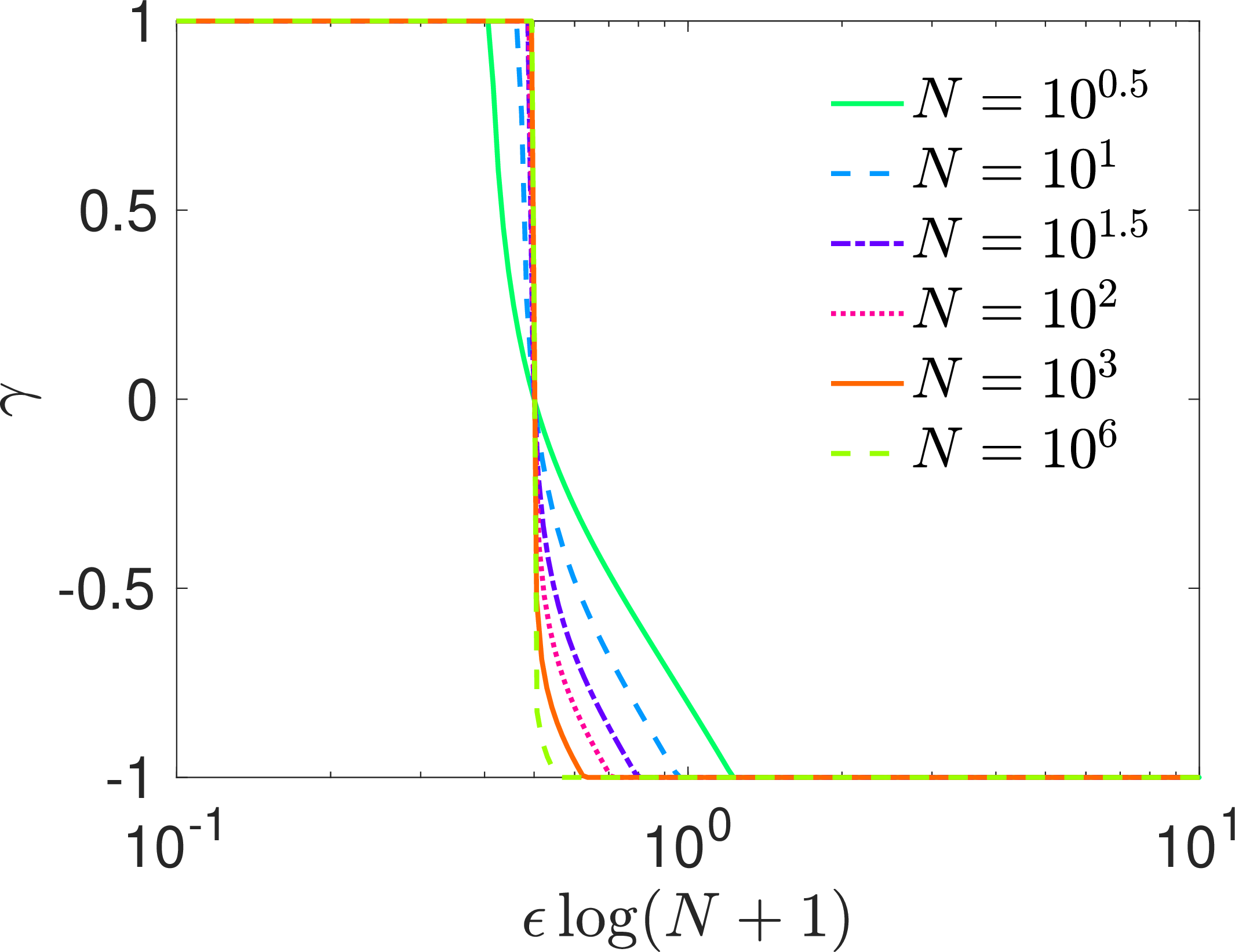
\end{align}\tag{8}\] which reduces at \(\gamma=0\) to the earlier result, as expected. Eq.@eq:lambdac entails modest dependence of the critical locus \(\lambda_*=1\) on \(\gamma\), but this locus is still primarily driven by varying \(\epsilon\) (at fixed \(N\)). Below we refer to the critical \(\epsilon\) obtained from this curve as \(\epsilon_c(\gamma)\) (Solving \(\lambda_*=1\) to obtain \(\epsilon_c(\gamma)\) is not
possible analytically, but easily obtainable numerically). As \(N \to \infty\) it becomes \(\epsilon_c(\gamma) \to 1/(2\log [N+1]),\) for \(\gamma>-1\). A
plot of this locus is shown in Fig.1 at varying \(N\); it separates \(\epsilon - \gamma\) space into two regions, which we will call the short-memory
phase \(\epsilon>\epsilon_c\) and the long-memory phase \(\epsilon<\epsilon_c\).
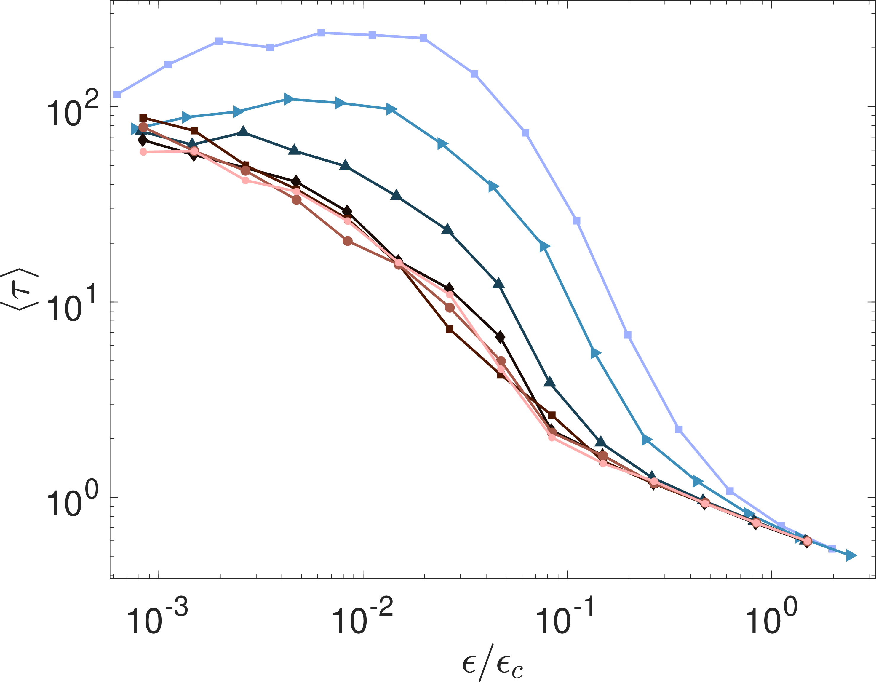
Note that the rigorous results from random matrix theory apply only to the case when the ensemble parameters are fixed as \(N \to \infty\); our arguments follow from the expectation that the \(N \to \infty\) results are obtained smoothly as \(N\) increases, as observed numerically. We expect that our prediction of a transition at \(\epsilon_c(\gamma; N)\) can be obtained rigorously by a distinguished limit in which \(N \to \infty\) while \(\epsilon/\epsilon_c\) remains finite, but this remains to be shown. So, we first show that the ensemble predictions are confirmed numerically. We validate Eq.@eq:lambdac by direct simulation across \((\epsilon,\gamma)\) and find good agreement for the onset of spectral reorganization (Fig. 2) and relaxation-time growth (Fig. 3).
The ensemble defined by Eq.@eq:lognormal yields transition rate matrices that are not necessarily symmetric, except in the limit \(\gamma \to -1\); their eigenvalues are therefore complex in general. Example transition rate spectra from this ensemble are shown in Fig.2, at varying \(\epsilon\) and \(\gamma\). As predicted, as \(\epsilon\) decreases, the filled ellipse of eigenvalues increases in size until its largest real part hits unity, at which point the spectrum reorganizes to form bicycle spokes. For \(\gamma<0\) one can see the flattening of the spectrum along the real axis, since as \(\gamma\to -1\) the transition matrices become symmetric. Instead for \(\gamma>0\) the effect of matrix asymmetry is mainly visible at large \(\epsilon\), where it elongates the ellipse.
More insight is gained from marginal distributions. As shown in Ref.[14], \(P(|\lambda|)\) develops a peak at \(|\lambda|=1\) as \(\epsilon \to \epsilon_c^+\), and further into the long-memory phase, which signals the arrival of long relaxation times. We plot in Fig.3 the expected relaxation time \(\tau = -1/\log |\lambda|\). This grows as \(\epsilon\) decreases, but more steeply for smaller \(\gamma\), that is when transition matrices are more symmetric.
1.3 Entropy Production↩︎
In the framework of stochastic thermodynamics [29], the ratio of forward and backward transition rates of a continuous-time Markov chain satisfies \[\begin{align} k_B \log \frac{W_{ij}}{W_{ji}} = \Sigma_{j \to i} , \end{align}\] where \(\Sigma_{j \to i}\) is the entropy produced in the transition from \(j\) to \(i\), and \(k_B\) is Boltzmann’s constant. This holds when the transitions are caused by energy exchange with a reservoir in thermodynamic equilibrium, and all internal degrees of freedom of the system are well equilibrated. Applied to a coarse-grained model, \(\Sigma\) computed from this formula lower-bounds the true entropy production of the transition. The expected value of the total entropy production rate is \[\begin{align} \label{Sigma} \dot{\Sigma} = k_B \sum_{i,j} W_{ij} \pi_j \log \frac{\pi_j W_{ij}}{\pi_i W_{ji}} . \end{align}\tag{9}\] where \(\pi_j\) is the stationary probability in state \(j\). Although Eq.@eq:Sigma has a strict interpretation only under the conditions of stochastic thermodynamics, it is a convenient measure of broken detailed balance for any Markov process, because it vanishes if and only if the process is in detailed balance, i.e. when \(\pi_j W_{ij} = \pi_i W_{ji}\) for all \(i,j\).
To apply this to discrete-time Markov chains, we note that any continuous-time Markov chain can be embedded as a discrete-time Markov chain with \(M_{ij} = W_{ij}/\sum_{k \neq j} W_{kj}\). Going in the reverse direction is nontrivial in general [30], [31].
For simplicity, we define a discrete-time analog of entropy production using Eq.@eq:Sigma , but with \(W_{ij} \to M_{ij}\), giving an entropy production rate in units of the time step of the discrete-time chain.
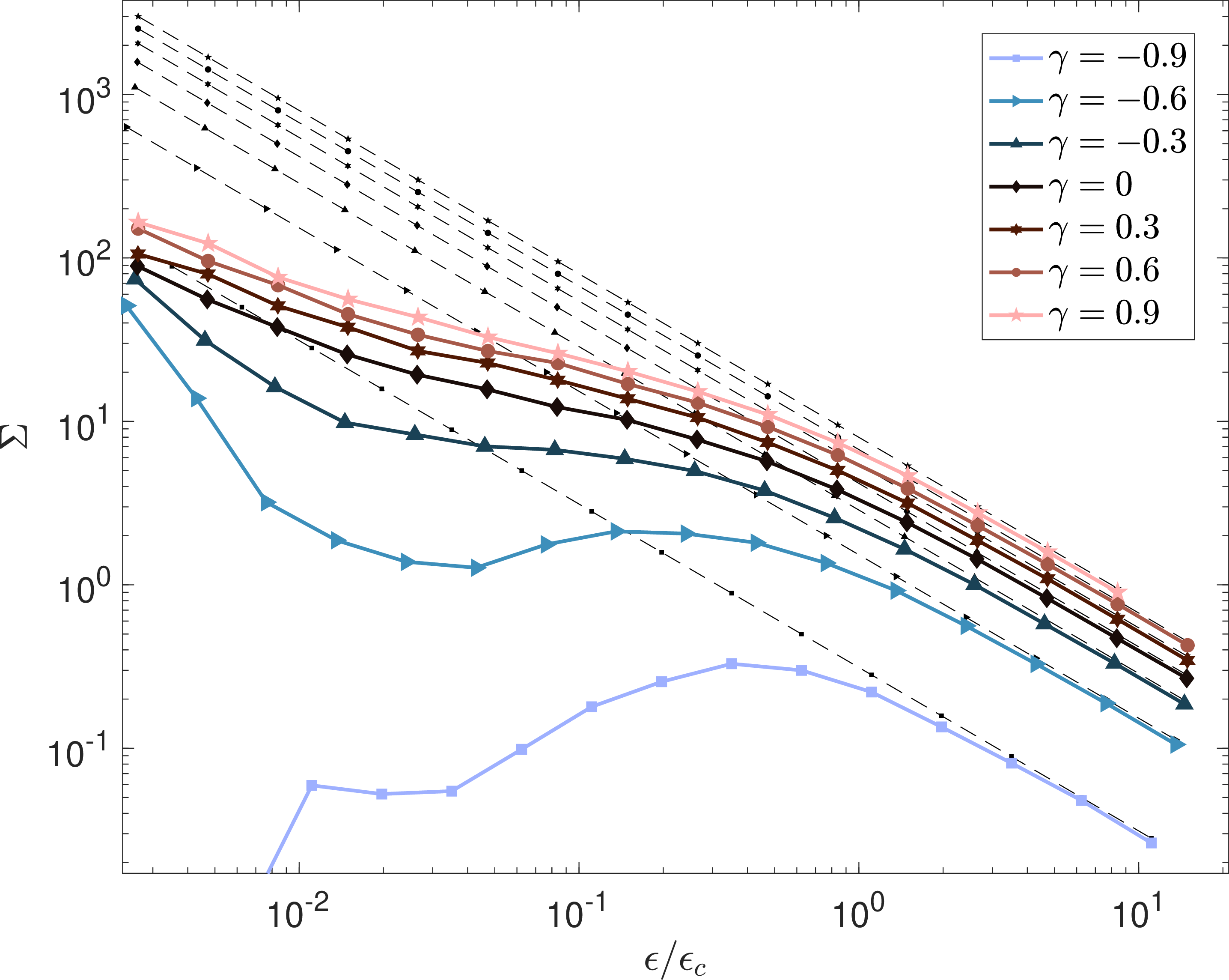
Fig.4 shows \(\langle \dot{\Sigma} \rangle\) over the ensemble at indicated \(\gamma\) and \(N=64\), in units with \(k_B=1\). A simple large-\(\epsilon\) estimate is obtained by approximating \(\pi_i \approx 1/N\) and \(M_{ij}\approx Q_{ij}/N\langle Q\rangle\), leading to 1 \[\begin{align} \label{Sigma95th} \langle \dot{\Sigma} \rangle/k_B \approx \frac{1+\gamma}{2\epsilon} \qquad \text{for } \epsilon \gg 1 \end{align}\tag{10}\] As shown by the dotted lines in Fig.4, this captures \(\langle \dot{\Sigma} \rangle\) for \(\epsilon \gtrsim \epsilon_c\). For smaller \(\epsilon\), we see that when \(\gamma<0\), the entropy production actually peaks below \(\epsilon_c\).
1.4 Predictive information↩︎
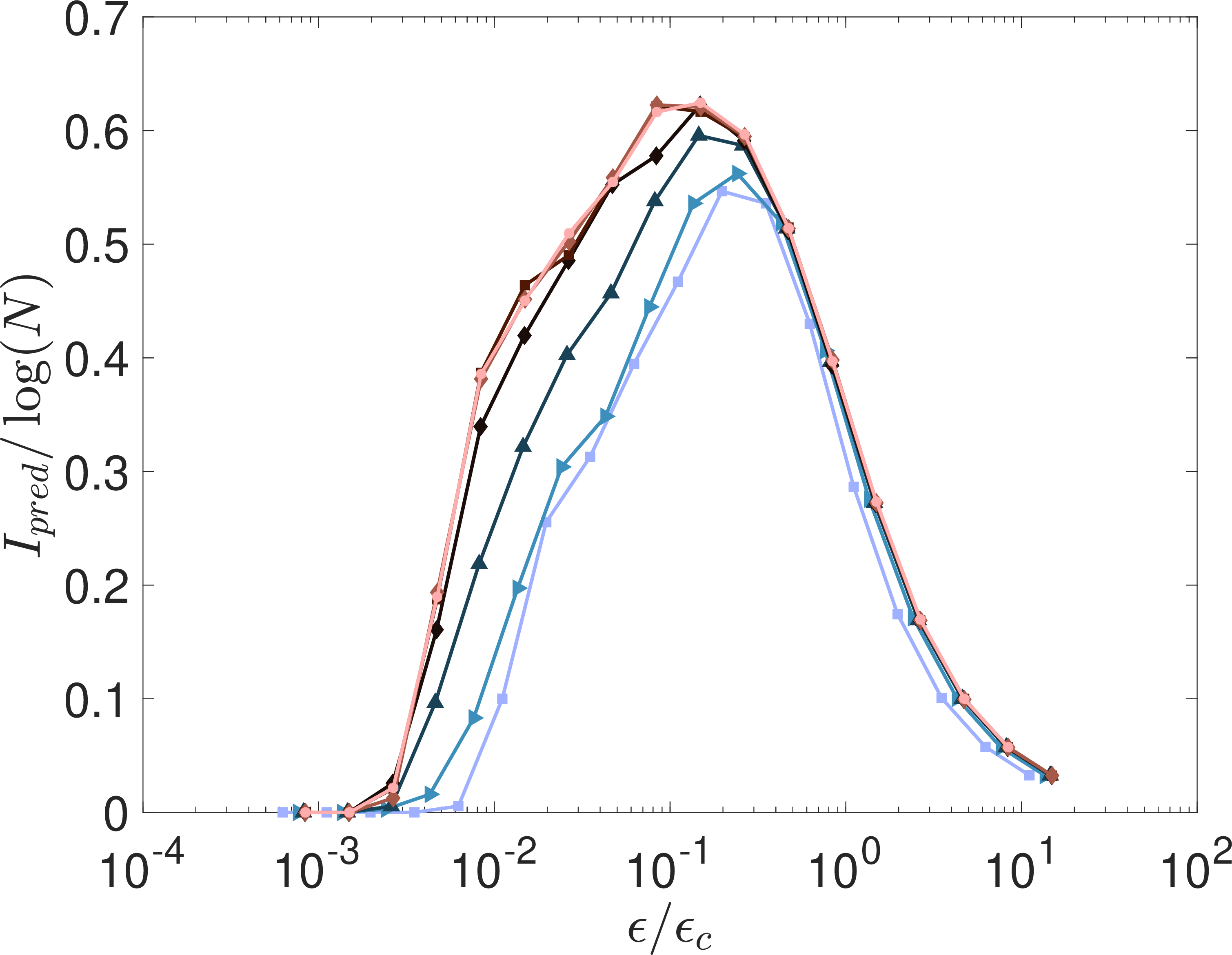
Figure 5: Predictive information as a function of \(\epsilon/\epsilon_c(\gamma)\), at various \(\gamma\) from \(-0.9\) (light blue) to \(+0.9\) (pink); symbols as in Fig.4, and \(N=64\)..
The non-monotonic dependence of entropy production recalls a result shown in [14], wherein the \(\gamma=0\) ensemble was shown to be non-monotonic in predictive information, a measure of complexity [33], [34].
We recall its definition. Consider the Shannon entropy of a sequence of length \(t\), \(H(t)\), measured in nats. We assume a stationary process. The entropy rate is defined as the extensive part, i.e. \[\begin{align} H_d = \lim_{t \to \infty} \frac{1}{t} H(t) \end{align}\] The predictive information is obtained as follows. Consider the mutual information between the ‘past’ and the ‘future,’ which measures how much the past is informative about the future. This is \(I(t,t') = H(t) + H(t') - H(t+t')\) for a past of length \(t\) and future of length \(t'\). The predictive information in nats is defined as \[\begin{align} I_{\text{pred}}(t) = \lim_{t' \to \infty} I(t,t'), \end{align}\] For a stationary Markov process it can be written [14] \[\begin{align} I(t,t') = H_\pi - H_d \label{I} \end{align}\tag{11}\] where \(H_\pi\) is the Shannon entropy of the stationary distribution, which is assumed to exist. This is independent of both \(t\) and \(t'\), a non-generic property [33], [34]. Thus in this setting predictive information is effectively a single-number summary of stationary structure, rather than a scale-dependent complexity measure.
The predictive information is shown in Fig. 5. This peaks near \(\epsilon/\epsilon_c \approx 0.1 - 0.3\), depending on \(\gamma\). Comparing with the result for \(\Sigma\), for \(\gamma<0\), we see that \(I_{\text{pred}}\) peaks at a smaller value of \(\epsilon/\epsilon_c\) than \(\Sigma\). Thus, even within this minimal null model, maximizing predictive information is distinct from maximizing entropy production.
We note that \(I_\text{pred}\) is proportional to \(\log N\) for \(\epsilon > \epsilon_c\), while approximately proportional to \(\log^2 N\) for \(\epsilon < \epsilon_c\), when plotted versus \(\epsilon/\epsilon_c\) (see [14]).
1.5 Variability at criticality↩︎
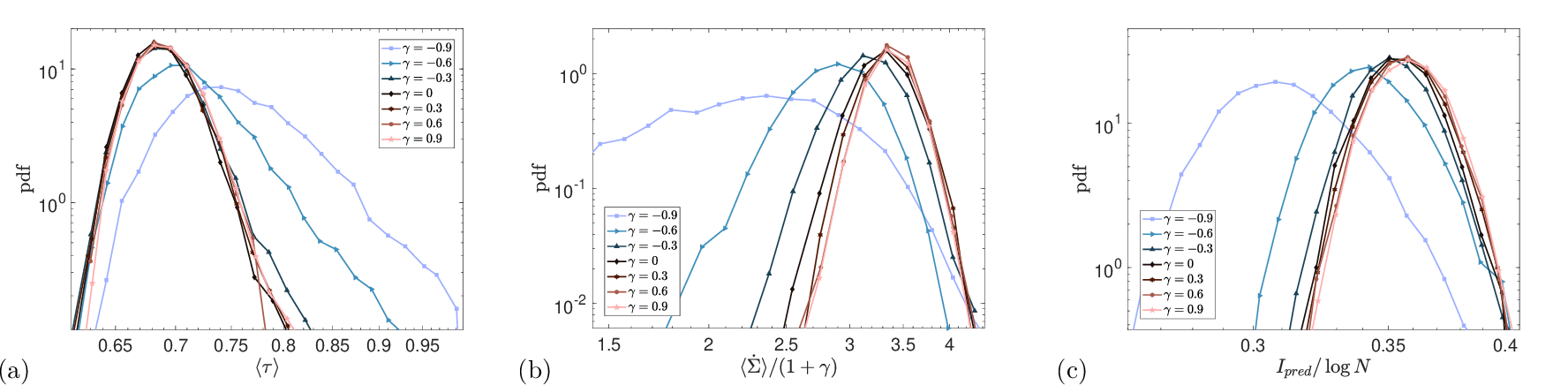
Figure 1 indicates that the system operates closest to criticality in the vicinity of \(\epsilon \log (N+1) = 1/2\), with some deviations at smaller \(N\) for \(\gamma\rightarrow-1\) and \(\gamma\rightarrow1\). Although this value defines the critical point, the associated dynamical and informational quantities are not single, fixed values. Instead, substantial variability may be observed, reflecting the fluctuations characteristic of systems near a critical transition. Figure 6a shows the distribution of relaxation times \(\tau\) at \(\epsilon=\epsilon_c(\gamma)\) and \(N=64\). The corresponding distributions of the entropy production rate \(\Sigma\) and the predictive information \(I_{\mathrm{pred}}\) are shown in Figures 6b and 6c, respectively. As seen in the three figures, variability in the respected quantities is approximately independent of \(\gamma\), except as the symmetric limit is approached (\(\gamma \to -1\)).
2 Applications↩︎
2.1 Parameter inference↩︎
To apply this ensemble to applications, we need to infer the values of \(\epsilon\) and \(\gamma\) from data; we will use maximum likelihood estimation (MLE). We assume that the data provides a discrete-time Markov model. For neurological data, such a model can be built with the Hidden Markov Multivariate Autoregressive (HMM-MAR) package [15], [17], [35]. Briefly, this package allows for multivariate time series data to be segmented into discrete states that are characterised by spectral properties.
The log-likelihood is the log-probability of the data, given the parameters, considered as a function of the parameters. In our ensemble this is:
\[\begin{align} \label{MLE} \mathcal{L}(\epsilon,\gamma,q) & = \log \prod_{a<b} \frac{1}{Z Q_{ab} Q_{ba}} e^{-\epsilon' \log^2(Q_{ab}/q)} e^{-\epsilon' \log^2(Q_{ba}/q)} e^{-2 \gamma \epsilon' \log(Q_{ab}/q) \log(Q_{ba}/q)} \prod_a \frac{1}{Z_0 Q_{aa}} e^{-\epsilon \log^2(Q_{aa}/q)} \notag \\ & = {\mathcal{L}}_0 -\frac{N(N-1)}{2} \log Z - \epsilon' \sum_{a \neq b} \log^2(Q_{ab}/q) - 2\gamma \epsilon' \sum_{a < b} \log(Q_{ab}/q) \log(Q_{ba}/q) - N \log Z_0 - \epsilon \sum_a \log^2(Q_{aa}/q) \notag \\ & = {\mathcal{L}}_0 -\frac{N(N-1)}{2} \log Z - \epsilon' N^2 h(Q; q) - 2\gamma \epsilon' \frac{N(N-1)}{2} a(Q; q) - N \log Z_0 + (\epsilon'-\epsilon) N d(Q; q) \end{align}\tag{12}\] where \(d(Q; q) = \frac{1}{N} \sum_a \log^2(Q_{aa}/q)\), and we recall that \(\epsilon' = \epsilon/(1-\gamma^2)\). Here \(Z = (\pi/\epsilon) \sqrt{1-\gamma^2}\), \(Z_0 = \sqrt{\pi/\epsilon}\), and \(\mathcal{L}_0\) is a constant. Note that the diagonal elements are treated such that \(P(Q_{aa})\) is the same as the marginal \(P(Q_{ab})\); this accounts for the different prefactors \(\epsilon\) vs \(\epsilon'\) in the two cases.
Maximizing \(\mathcal{L}\) with respect to the three parameters \(\epsilon, \gamma,\) and \(q\) leads to the MLE equations \[\begin{align} \tag{13} \epsilon & = \frac{N(1-\gamma^2)/2}{Nh + \gamma (N-1) a - \gamma^2 d} \\ \gamma & = \frac{-B - \sqrt{B^2 - 8a^2(N-1)(Nh\epsilon+d\epsilon-N)}}{2a(N-1)} \tag{14} \\ \log q & = \frac{\sum_{a,b} \log Q_{ab} - \gamma \sum_a \log Q_{aa} }{N(N-\gamma) } \tag{15} , \end{align}\]
with \(B = \frac{(Nh-d)(-1+ 4d\epsilon-N)}{N-1} + 2a^2 \epsilon (N-1)\).
We solve these equations by iteration, beginning with the guess \(\gamma=0\) and iterating through equations for \(q\), \(\epsilon\), and \(\gamma\), in that order. We confirmed that in the ensemble, this procedure successfully reproduces imposed parameter values over the full range of parameters needed (down to \(\epsilon= 10^{-2}\)).
2.2 Human fMRI data↩︎
First, we revisit a dataset of task-free resting state fMRI data from the Human Connectome project [36] previously analyzed in [14] assuming \(\gamma=0\). The data is of 820 healthy adults aged 22-35 years, including 453 females. All subjects are anonymized, and the recordings reflect fMRI activity during wakeful rest. \(N\) varies from \(N=5\) to \(N=12\) with a mean value \(N \approx 11.4\).
In [14], it was found that the data were well-characterized by \(\epsilon \approx \epsilon_c\), without fitting parameters. Additionally, it was shown that the Shannon entropy, predictive information, and various spectral measures of the data were all well-predicted by their values in the ensemble of Markov models, given only the measured values of \(N\) and \(\epsilon\) and the probability to remain in the same state from one time step to the next.
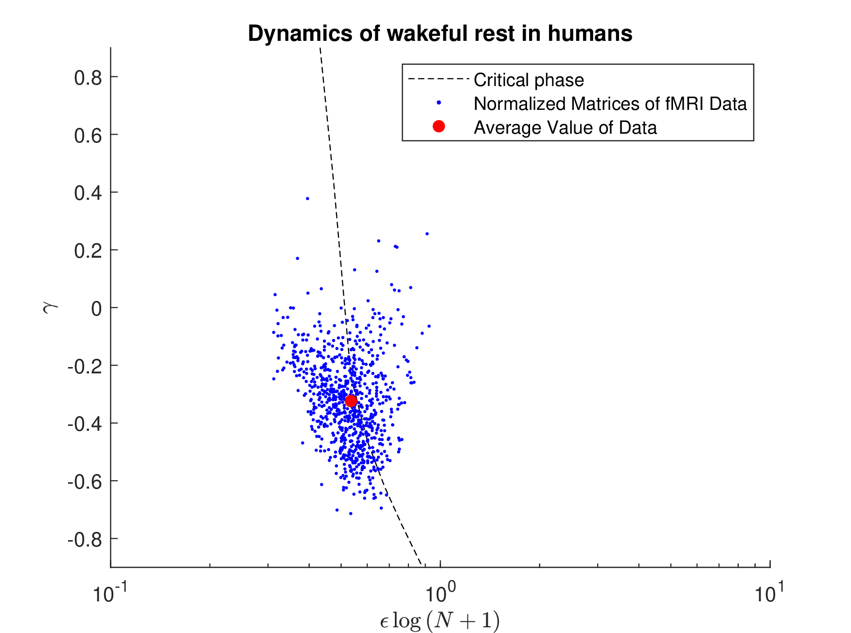
Here we analyze this dataset in the larger \(\epsilon-\gamma\) ensemble, obtained by MLE. The resulting phase space distribution is shown in Fig. 7. In agreement with [14], we find that the mean value of the data lies very close to the critical locus, i.e. \(\epsilon \approx \epsilon_c\), with \(\epsilon_c\approx0.2\) and the mean value for \(\gamma\) lies at \(\gamma\approx-0.4\). There is substantial variability in \(\gamma\).
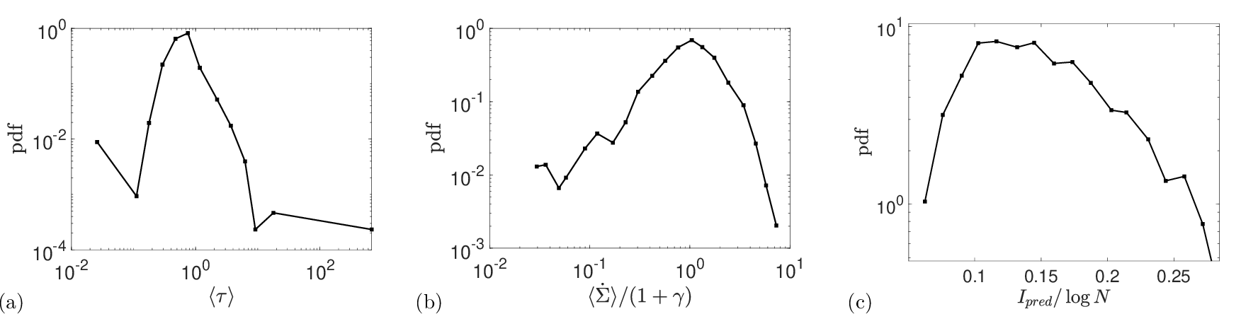
Although the subjects varied in age and gender, we cannot regress these variables with \(\epsilon\) or \(\gamma\) as the dataset was anonymized before release to the public. We can however test whether the variability in derived quantities matches that expected from the ensemble, shown in Fig.6. In Fig.8 we show the distributions of the corresponding quantities measured from the human fMRI ensemble.
Comparing Figure 6a with Figure 8a, we see that the values peak at \(\langle\tau\rangle\approx 0.68\) for the ensemble data, and at \(\langle\tau\rangle\approx 0.7\) for the human data. Figure 6b peaks at \(\langle\dot{\Sigma}\rangle/(1+\gamma)\approx 3.2\) for \(\gamma=-0.3\) whereas Figure 8b appears to peak at \(\langle\dot{\Sigma}\rangle/(1+\gamma)\approx 1\). For predictive information, there is a peak in Figure 6c at \(I_\text{pred}/\log N\approx 0.35\) whereas the human data shown in Figure 8c has a broad shoulder from \(I_\text{pred}/\log N \approx0.1\) to \(I_\text{pred}/\log N \approx 0.15\). To compare variability, we measure the full width at 10% of the maximum and express it as a ratio of the largest value taken to the smallest value. For the ensemble, we find widths of \(\approx 1.15, 1.47\) and \(1.2\) for \(\tau, \dot{\Sigma}/(1+\gamma),\) and \(I_\text{pred}\), respectively, at \(\gamma=-0.3\). In the human fMRI ensemble, the corresponding values are \(\approx 10, 15,\) and \(4.4\): the human data displays significantly more variability than expected from the ensemble, the null model. Therefore the spread of data in Figure 7 does not reflect natural variability amongst transition rate matrices at any putative value of \(\epsilon, \gamma\) and modest \(N\), but instead evidences individual differences amongst subjects.
Overall, this example validates the enlarged ensemble, showing that it adds extra information without destroying the parsimony of the simpler \(\gamma=0\) ensemble. In addition to quantities shown in [14] to be well predicted by the ensemble (Shannon entropy, and eigenvalue distributions), the mean relaxation time is well predicted by the ensemble, while the data is significantly less dissipative (smaller \(\dot{\Sigma})\) and slightly less informative (smaller \(I_{\text{pred}}\)) than expected from the ensemble. In addition, the human fMRI data shows enhanced variability around these means.
2.3 Human EEG data↩︎
Next, we analyze a dataset of individuals with Alzheimer’s disease, frontotemporal dementia, and healthy controls, outlined in [37]. The data is of resting state EEG recordings of 88 adults and includes further information regarding age, group (Alzheimers, Dementia, or control), and gender. All subjects in this analysis have been anonymized and the data reflects brain activity measured by scalp EEG during wakeful rest without specification due to any of the above factors.
The raw data was in the form of 19 scalp electrodes with 2 reference electrodes with a sampling rate of 500Hz and \(10\text{uV/mm}\) resolution (see [38]). First, 5 regions were defined based on the positions of the scalp electrodes and the data was partitioned into windows that were \(15000\) time steps long. The regions represented the frontal, central, temporal, parietal, and occipital regions of the brain. To process the data into Markov models, a toolkit developed for building Markov models from neurological data was utilized [15], [39]–[44]. Each of the \(R=5\) regions was processed with the HMMMAR toolkit for each window with \(S=4\) states per region. Once state sequences were found, they were recombined to form a larger model with a maximum of \(S^R=1024\) possible states. State sequences were then used to construct transition matrices for the Markov models which statistics were calculated from.
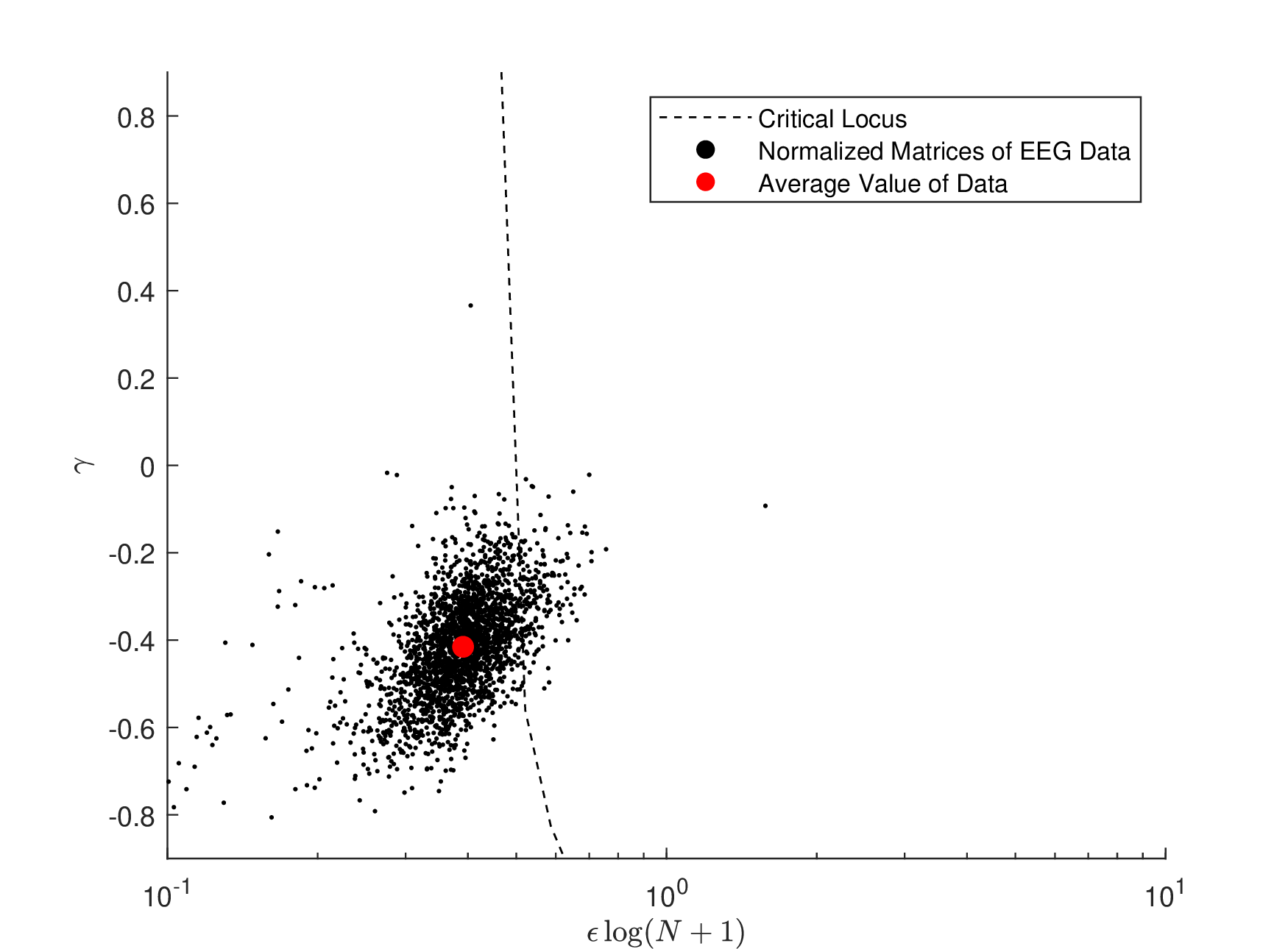
Figure 9 shows the inferred values of \(\epsilon\) and \(\gamma\) as a scatter plot of subject values. All subjects, both diseased and healthy, are included; we did not find any systematic differences between them. The mean value of \(\epsilon \log (N+1)\) was \(0.39\), the mean \(\gamma\) was \(-0.42\), and the mean size of the transition matrices was \(N=165\). This is comparable to the fMRI data which had mean values \(\epsilon\log (N+1) \approx 0.53\) and \(\gamma \approx -0.32\), despite being analyzed at a much smaller value of \(N\). In both cases, the human data falls just to the left of the critical line.
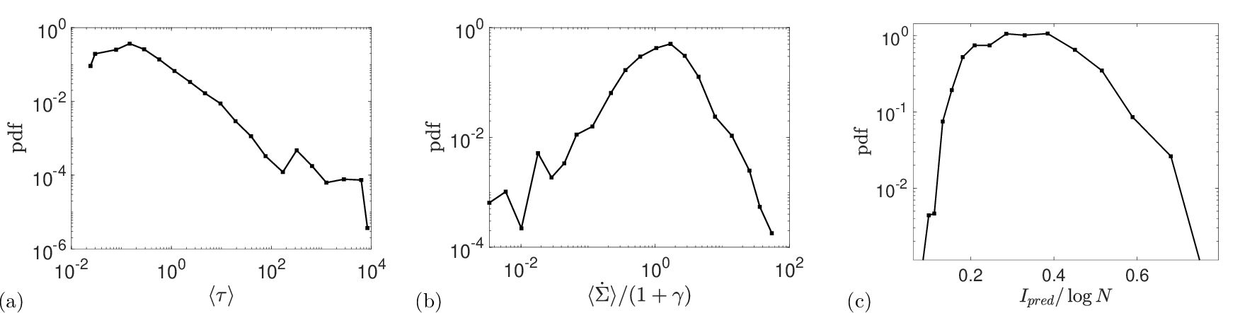
Figure 10a-c shows histograms of \(\tau\), \(\dot{\Sigma}/(1+\gamma)\), and \(I_\text{pred}/\log N\) respectively. \(\tau\) peaks at about \(10^{-1}\), which is much lower than the peak shown in Figure 6a, although still within the expected range. \(\dot{\Sigma}\) peaks at \(\dot{\Sigma}/(1+\gamma)\approx 1.7\), smaller than expected from Figure 6b. \(I_\text{pred}/\log N\) has a broad distribution ranging from \(I_\text{pred}/\log N\approx 0.2\) to \(I_\text{pred}/\log N\approx 0.4\), capturing the ensemble value of 0.35.
We have compared \(I_\text{pred}\) when scaled by \(\log N\), which is appropriate for \(\epsilon > \epsilon_c\). For \(\epsilon < \epsilon_c\), \(I_\text{pred}\) scales approximately as \(\log^2 N\) (see Fig. 5c in [14]). This additional factor would change the comparison between datasets to \(I_\text{pred}/\log^2 N \approx 0.08\) (ensemble), \(I_\text{pred}/\log^2 N \approx 0.05\) (fMRI), and \(I_\text{pred}/\log^2 N \approx 0.06\) (EEG), bringing them even closer together.
Overall, the two datasets of human data, measured with very different techniques (fMRI vs EEG), are remarkably similar when considered as Markov models in the \(\epsilon-\gamma\) ensemble. Considering the expansive range of observables within the ensemble, for example of relaxation time (Fig. 3) and of entropy production (Fig. 4), which each vary over many decades as \(\epsilon\) and \(\gamma\) vary, the human datasets are similar both to each other, evidencing a super-universality of human criticality, and similar to the null-model expectations from the ensemble.
The main difference between measured data and ensemble expectations, considered for simplicity as that at a single representative \((\epsilon,\gamma)\), is that the measured data has significantly higher variability. This variability cannot be explained by expected variance within the ensemble: subject-to-subject variability is instead implicated. The detailed investigation as to why the human data has deviations from the ensemble data, both in mean and variance, is left for a future study.
3 Conclusion↩︎
We presented a null model for the analysis of discrete-time Markov models. The \(\epsilon-\gamma\) ensemble captures the expected behavior of entropy production, Shannon entropy, relaxation time, and predictive information, and can be used to infer the behavior of these observables in real data sets.
The ensemble captures a notion of criticality, measured by \(\epsilon-\epsilon_c(\gamma; N)\), and a notion of nonequilibrium, measured by \(\gamma\). A key result is that many observables depend strongly on \(\epsilon\) but weakly on \(\gamma\), away from the \(\gamma=-1\) limit that corresponds to symmetric transition rate matrices. Specifically both the mean relaxation time \(\tau\) (Fig.3) and predictive information \(I_{\text{pred}}\) (Fig.5) display weak \(\gamma\) dependence. Even the entropy production rate \(\dot{\Sigma}\), which is nominally a function of \(\gamma\), depends much more strongly on \(\epsilon\) than \(\gamma\) (Fig.4). Beyond supporting the original model of [14], this has the following consequence: In this null model, inferring degree of nonequilibrium from scalar irreversibility metrics alone is ill-conditioned because heterogeneity confounds it; robust inference of \(\gamma\) requires either direct pairwise forward/backward statistics, or cycle-based metrics.
Moreover, this means that distance from criticality and measures of nonequilibrium are in practice strongly correlated. Importance of observables conventionally associated with one should not be used to disregard the other. Our results suggest that empirical increases in irreversibility measures need not imply stronger microscopic time-asymmetry, but may instead reflect increased dynamical heterogeneity [3]–[5].
As an application we tested the ensemble on two datasets of humans at wakeful rest, measured with fMRI and EEG. The datasets support the brain criticality hypothesis, extending previous results in the \(\gamma=0\) ensemble. Moreover the two datasets are quantitatively similar in their placement in the \(\epsilon-\gamma\) plane, supporting a super-universality of human brain criticality: whole-brain resting dynamics appear to be constrained to a low-dimensional manifold in Markov-model space (approximately the vicinity of the critical locus with moderately negative \(\gamma\)), suggesting strong macro-constraints on effective dynamics independent of measurement technology. Our data are consistent with a predictive information \(I_\text{pred} \approx 0.05 \log^2 N\) measured in nats, for a model with \(N\) visited states.
The enlarged \(\epsilon-\gamma\) plane (compared to the \(\gamma=0\) ensemble of [14]) allows, in principle, discrimination between various objectives, such as maximizing entropy production, or maximizing predictive information. This will be addressed in a future work studying the behavior of monkeys
under tasks.
Acknowledgments: EDG is supported by NSERC Discovery Grant RGPIN-2020-04762.