Achieving Linear Speedup for Composite Federated Learning
January 01, 1970
Abstract
This paper proposes FedNMap, a normal map-based method for composite federated learning, where the objective consists of a smooth loss and a possibly nonsmooth regularizer. FedNMap leverages a normal map-based update scheme to handle the nonsmooth term and incorporates a local correction strategy to mitigate the impact of data heterogeneity across clients. Under standard assumptions, including smooth local losses, weak convexity of the regularizer, and bounded stochastic gradient variance, FedNMap achieves linear speedup with respect to both the number of clients and the number of local updates for nonconvex losses, both with and without the Polyak-Łojasiewicz condition. To the best of our knowledge, this is the first algorithm establishing linear speedup for nonconvex composite federated learning. Numerical experiments corroborate our theoretical findings and demonstrate the linear speedup of FedNMap.
distributed optimization, nonsmooth optimization, stochastic optimization, federated learning, normal map
1 Introduction↩︎
Federated learning (FL) enables a set of clients to collaboratively train a global model, enhancing computational efficiency through parallel local training [1], [2]. While the theory of FL algorithms for smooth objective functions is well developed, many applications involve a nonsmooth regularization term \(\varphi:\mathbb{R}^p \rightarrow(-\infty, \infty]\). Typical examples include statistical learning with sparsity-inducing norms [3], constrained optimization [4], and model pruning [5]. These applications motivate the following distributed composite optimization problem: \[\label{eq:P} \min_{x\in \mathbb{R}^p} \psi(x):= f(x) + \varphi(x),\; f(x) := \frac{1}{n}\sum_{i=1}^nf_i(x),\tag{1}\] where each client \(i\) has access only to its local objective function \(f_i:\mathbb{R}^p\rightarrow\mathbb{R}\) and the (possibly nonsmooth) regularizer \(\varphi:\mathbb{R}^p\rightarrow (-\infty, \infty]\).
In this work, we assume \(\varphi\) is proper, lower semicontinuous, lower bounded, and \(\rho\)-weakly convex, and each \(f_i\) is \(L\)-smooth on an open set containing \(\{x\in\mathbb{R}^p: \varphi(x)<\infty\}\). We further assume each client \(i\) can query an unbiased stochastic gradient \(g_i(x;\xi_i)\) (\(\xi_i\) is a random variable) of \(\nabla f_i(x)\) with bounded variance, and that the proximal operator \[\begin{align} \mathrm{prox}_{\gamma\varphi}\left(x\right):= \arg\min_{y\in\mathbb{R}^{p}} \varphi(y) + \frac{1}{2\gamma}\Vert y-x \Vert^2, \end{align}\] is computationally tractable for \(\gamma>0\).
For smooth problems, e.g., \(\varphi(x)\equiv0\), a line of work has established the linear speedup property [6]–[8]. Specifically, to reach a sufficiently small target accuracy, using \(n\) clients and \(Q\) local steps reduces the number of communication rounds by a factor of \(\mathcal{O}\left(nQ\right)\). In contrast, achieving linear speedup for the composite FL problem 1 remains largely underexplored. Although several recent works [3], [9]–[11] propose proximal FL methods for solving 1 , significant gaps remain. These methods either (i) focus only on convex or strongly convex regimes [3], [10], [12], (ii) require additional restrictive conditions such as homogeneous objectives [12] or bounded subgradients of \(\varphi\) [10], [11], or (iii) fail to establish convergence results for general nonconvex composite objectives [9], [11]. Consequently, it remains unclear whether linear speedup can be achieved for general composite FL under standard assumptions. This motivates the central question of our work:
Can we design an FL method that achieves linear speedup for solving the composite FL problem 1 under standard assumptions?
In this paper, we give an affirmative answer to this question. A critical challenge in solving problem 1 arises from the nonlinearity of the proximal operator. In particular, the proximal stochastic gradient descent (Prox-SGD) update: \(x_{t + 1} = \mathrm{prox}_{\eta \varphi}(x_t - \eta g (x_t;\xi_t))\) [13], [14] can introduce bias, since \(\mathbb{E}\left[x_{t + 1}|x_t\right] \neq \mathrm{prox}_{\eta \varphi}(x_t - \eta \nabla f(x_t))\) even when the stochastic gradient is unbiased. This inconsistency becomes particularly pronounced for FL methods with \(Q>1\) local steps. To address this challenge, we leverage a so-called normal map-based update scheme [15], [16] that preserves unbiasedness. The proposed method, denoted FedNMap, integrates the normal map update scheme with a local correction term to mitigate the impact of data heterogeneity across clients. Under standard assumptions, we show that FedNMapachieves linear speedup for solving problem 1 under nonconvex losses, both with and without the Polyak–Łojasiewicz (PL) condition. Moreover, FedNMapdoes not require any assumptions on data heterogeneity.
1.1 Related Works↩︎
FL for minimizing smooth objective functions has been extensively studied [6], [7], [17]–[20]. FedAvg [6], [17] pioneered this line of work, but relies on restrictive assumptions of limited data heterogeneity. To mitigate this issue, several improved algorithms have been proposed. For instance, FedProx [19] introduces a proximal term into the local subproblem to stabilize training. FedPD [20] employs a primal-dual approach to enhance convergence, and SCAFFOLD [18] introduces two control variates to correct local updates. More recent work [7] establishes convergence of FedAvg without restrictive data heterogeneity assumptions and under a general variance condition.
Several recent works have studied composite FL. FedDA [12] employs dual averaging and establishes linear speedup for convex settings when the objective functions are homogeneous or quadratic. More recently, EcontrolDA [21] achieves linear speedup for convex heterogeneous objective functions but does not incorporate multiple local steps. For strongly convex objective functions, [10] establish convergence without linear speedup but requires bounded subgradients of the nonsmooth term. For nonconvex objective functions, it remains unclear whether convergence can be achieved under standard assumptions [9], [11]. Table 1 presents a detailed comparison of related works and their conditions.
Normal map-based methods [15] have been studied for solving composite problems, both in centralized settings [16], [22], [23] and in distributed settings [24]. Compared with classical proximal stochastic gradient descent (Prox-SGD) [13], [14], the normal map-based update scheme preserves unbiasedness when an unbiased stochastic gradient of the smooth component \(f\) is available. Furthermore, the normal map serves as a favorable stationarity measure for composite problems and recovers several classical stationarity measures [16].
| Method | \(f\) or \(\psi\) | \(\varphi\) | ||
| Assumptions | Convergence Rate | |||
| [12] | \(f\) CVX | CVX | \(\zeta\), Quadratic | \(\order{\sqrt{\frac{\sigma^2}{nQT}} + \frac{\zeta^{2/3} + \sigma^{2/3}/Q^{1/3}}{T^{2/3}}}\) |
| [21] | \(f\) CVX | CVX | \(Q=1\) | \(\order{\sqrt{\frac{\sigma^2}{nT}} + \frac{\sigma^{2/3}}{T^{2/3}} + \frac{1}{T}}\) |
| [3] | \(f\) SCVX | CVX | \(\zeta\), BI | \(\torder{\frac{\sigma^2}{T} + \frac{Q^2 (\zeta^2 + B^2)}{T^2} }\) |
| [10] | \(f\) SCVX | CVX | \(B_\psi\) | \(\torder{\frac{\sigma^2 + B_\psi^2}{nT}}\) |
| [9] | \(\psi\) PL | CVX | \(B_\psi\) | Not established |
| [11] | \(\psi\) PL | WCVX | \(B_\psi\) | Not established |
| (This work) | \(f\) NCVX | WCVX | / | \(\bs{\order{\sqrt{\frac{\sigma^2}{nQT}} + \frac{1}{T}}}\) |
| (This work) | \(\psi\) PL | WCVX | / | \(\bs{\torder{\frac{\sigma^2}{nQT} + \frac{\sigma^2}{T^2}}}\) |
1.2 Main Contribution↩︎
In this paper, we make the following key contributions to composite federated learning:
Linear speedup for nonconvex composite FL. We propose FedNMapalgorithm and show that it achieves linear speedup for nonconvex composite FL (Theorem 1). Specifically, FedNMapattains an \(\varepsilon\)-solution with communication complexity \[\begin{align} \mathcal{O}&\left(\frac{(L + \rho)\Delta_\psi\sigma^2}{nQ\varepsilon^4} + \frac{(L + \rho)\Delta_\psi}{\varepsilon^2}+ \frac{{\frac{1}{n}\sum_{i=1}^n\Vert \nabla f_i(x_0) \Vert^2 + L^2\Vert x_0-z_0 \Vert^2}}{\varepsilon^2}\right), \end{align}\] where \(\Delta_\psi := \psi(x_0) - \psi^*\), \(x_0 = \mathrm{prox}_{\gamma\varphi}(z_0)\), \(\psi^* := \inf_{x\in\mathbb{R}^p} \psi(x)\), and \(\sigma^2\) bounds the stochastic gradient variance.1 This result is comparable to previous results for smooth objectives with \(\varphi(x)\equiv0\), including SCAFFOLD [18], and exhibits a \(1/(nQ)\) dependence in the dominant term, demonstrating linear speedup with respect to both the number of clients \(n\) and the number of local steps \(Q\). By comparison, prior works have not established convergence results for the nonconvex composite setting (see Table 1).
Linear speedup under the PL condition. When \(\psi\) further satisfies the PL condition with modulus \(\mu\), FedNMapattains an \(\varepsilon\)-solution, i.e., \(\mathbb{E}\left[\psi(x_T) - \psi^*\right]\leq \varepsilon\), (Theorem 2) with communication complexity \[\begin{align} \tilde{\mathcal{O}}\left( \frac{(L+\rho)\sigma^2}{n Q \varepsilon\mu^2} + \sqrt{\frac{L^2 \sigma^2}{\varepsilon \mu (L + \rho + \mu)^2}}\right). \end{align}\] The dominant term again scales as \(1/(nQ)\), demonstrating linear speedup. In contrast, previous works assuming strongly convex objectives have not established such a result.
Mild assumptions. The convergence guarantees of FedNMaponly rely on the smoothness of \(f_i\), weak convexity of \(\varphi\), and bounded stochastic gradient variance. In contrast to several prior works, FedNMapdoes not require limiting assumptions on data heterogeneity or bounded subgradient assumptions [3], [10], [12].
Efficient communication. Despite handling composite objectives, FedNMap maintains communication load and memory cost comparable to those of state-of-the-art FL methods by using single-variable uplink communication, where each client sends only one variable to the server, thereby reducing the communication cost by \(50\%\) compared to SCAFFOLD.
1.3 Notation and Assumptions↩︎
All vectors are column vectors unless otherwise stated. Let \(x_{i,t}^\ell \in\mathbb{R}^p\) denote the iterate of client \(i\) at the \(\ell\)-th local update within the \(t\)-th communication round. We use \(\Vert \cdot \Vert\) to denote the Frobenius norm for matrices and the \(\ell_2\) norm for vectors. The notation \(\langle a, b \rangle\) stands for the inner product of two vectors \(a, b\in\mathbb{R}^{p}\). For a possibly nonsmooth function \(\psi\), \(\partial\psi(x)\) denotes the subdifferential set.
We next introduce the standing assumptions. Assumption 1 requires each client \(i\) to have access to an unbiased stochastic gradient of \(f_i\) with bounded variance.
Assumption 1. Each client \(i\) has access to an unbiased stochastic gradient \(g_i(x;\xi_i)\) of \(\nabla f_i(x)\), i.e., \(\mathbb{E}[g_i(x;\xi_{i})|x] = \nabla f_i(x)\), and there exists \(\sigma\geq 0\) such that for any \(i\in[n]:=\{1,2,\ldots, n\}\), \[\begin{align} \mathbb{E}\left[\left\Vert g_{i}(x;\xi_{i}) - \nabla f_i(x) \right\Vert^2\middle|x\right]&\leq \sigma^2. \end{align}\] In addition, the stochastic gradients are independent across clients at each \(t\geq 0\) and \(\ell = 0,1,\ldots, Q-1\).
Assumption 1 can be relaxed to the more general ABC condition [7], [8], [25]. The results in this work can be extended to that setting by following procedures similar to those in [24].
Assumption 2 is standard and requires each \(f_i\) to be smooth and the objective function \(\psi\) to be lower bounded.
Assumption 2. Each \(f_i:\mathbb{R}^p\rightarrow\mathbb{R}\) is \(L\)-smooth on \(\mathrm{dom}(\varphi):=\{x\in\mathbb{R}^p: \varphi(x)<\infty\}\), i.e., \(\Vert \nabla f_i(x) - \nabla f_i(x') \Vert\leq L\Vert x - x' \Vert\), \(\forall x,x'\in\mathrm{dom}(\varphi).\) In addition, \(\psi\) is bounded from below, i.e., \(\psi(x)\geq \psi^*:= \inf_{x\in\mathbb{R}^p} \psi(x)>-\infty\) for any \(x\in\mathbb{R}^p\).
Assumption 3 requires the regularizer \(\varphi\) to be weakly convex, which covers many commonly used regularizers such as the indicator function of a closed convex set and the \(\ell_1\) norm [14].
Assumption 3. The function \(\varphi: \mathbb{R}^{p} \rightarrow (-\infty, \infty]\) is \(\rho\)-weakly convex, lower semicontinuous, lower bounded, and proper.
Assumption 4 characterizes a generalized PL condition for the composite problem 1, which holds, for example, when \(f\) satisfies the PL condition and \(\varphi\) is convex. Condition ?? is also known as the proximal-PL inequality. Typical examples include Lasso regression [26].
Assumption 4. There exists \(\mu>0\) such that the function \(\psi(x)\) satisfies \[\begin{align} \label{eq:PL} 2\mu\left(\psi(x)-\psi^*\right) \leq \left[\mathrm{dist}\left(0, \partial \psi(x)\right)\right]^2, \end{align}\qquad{(1)}\] for all \(x \in \mathbb{R}^p\), where \(\psi^*= \inf_{x\in\mathbb{R}^p}\psi(x)\) and \(\mathrm{dist}(0, \partial\psi(x)) := \min_{v\in\partial\psi(x)}\Vert v \Vert\).
2 FedNMap: Federated Learning with Normal Map-Based Updates↩︎
In this section, we introduce FedNMap, a novel algorithm for solving the composite FL problem 1 . The design of FedNMapconsists of two main components: (i) a normal map-based update that addresses the nonsmooth term \(\varphi\), and (ii) a correction term that mitigates the drift induced by multiple local steps.
We start by defining the normal map \[\label{eq:norm95def} \mathrm{F}^{\gamma}_{\mathrm{nor}}(z):= \nabla f(\mathrm{prox}_{\gamma\varphi}\left(z\right)) + \gamma^{-1}\left(z - \mathrm{prox}_{\gamma\varphi}\left(z\right)\right).\tag{2}\] Based on the second prox theorem [27], it holds that \(\mathrm{F}^{\gamma}_{\mathrm{nor}}(z)\in\partial\psi(\mathrm{prox}_{\gamma\varphi}\left(z\right))\). By defining the auxiliary variable \(x=\mathrm{prox}_{\gamma\varphi}\left(z\right)\) and letting \(g(x;\xi)\) be an unbiased stochastic gradient of \(\nabla f(x)\), we have \[\begin{align} \mathbb{E}\left\{g(x;\xi) + \gamma^{-1}\left(z - x\right)\middle| x,z\right\} &= \nabla f(x) + \gamma^{-1}\left(z - x\right)= \mathrm{F}^{\gamma}_{\mathrm{nor}}(z). \end{align}\] Therefore, the unbiasedness of the stochastic gradient is preserved, and we can leverage a corrected stochastic normal map update to perform local updates at each client.
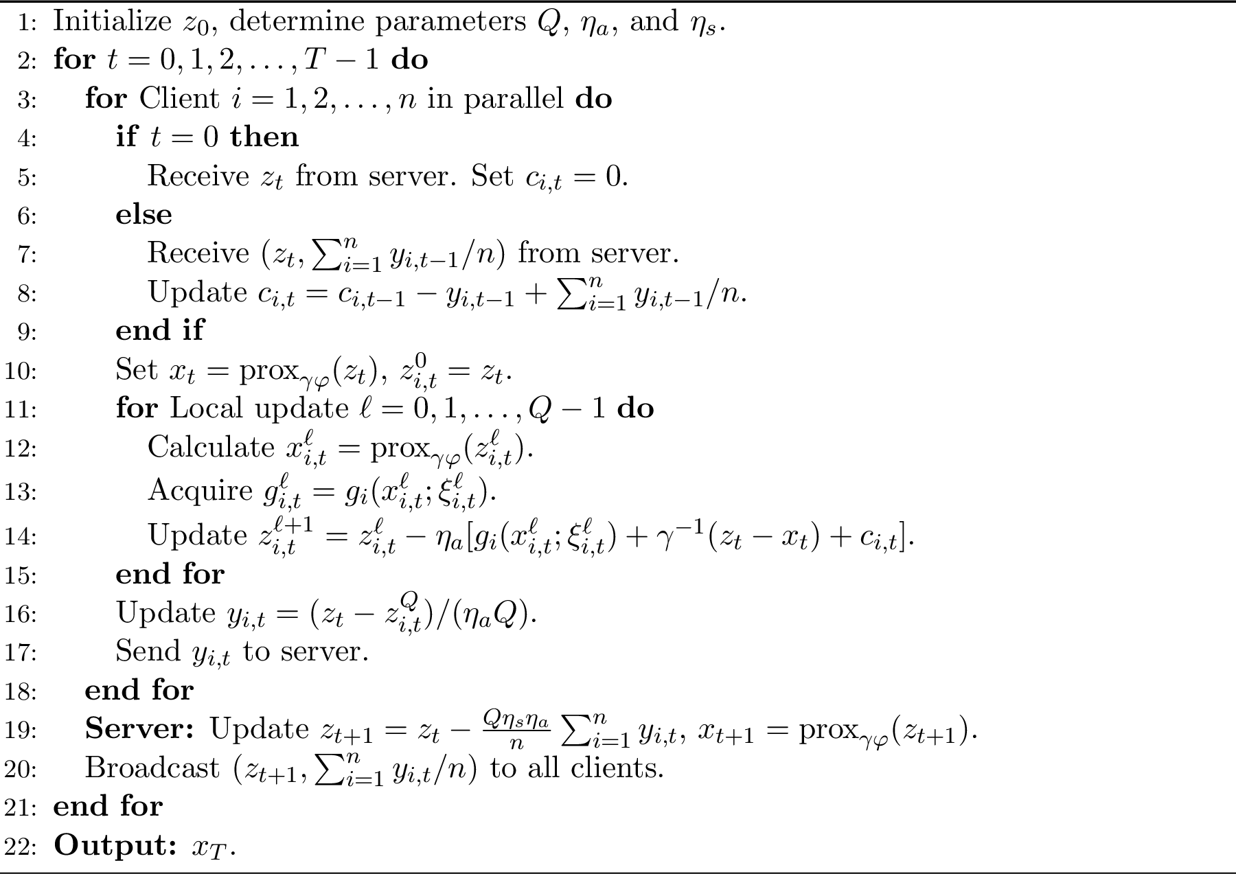
Client update. At communication round \(t\geq 1\), each client \(i\) receives \(z_t\) and the aggregated direction \(\frac{1}{n}\sum_{j=1}^n y_{j,t-1}\) from the server. The client sets \(x_{t} = \mathrm{prox}_{\gamma\varphi}\left(z_t\right)\) and initializes its local variable as \(z_{i,t}^0 = z_t\). The correction term \(c_{i,t}\) is updated according to \[c_{i, t } =\begin{cases} 0,& t=0\\ c_{i,t-1} - y_{i,t-1} + \frac{1}{n} \sum_{j=1}^ny_{j,t-1},& t\geq 1.\\ \end{cases}\label{eq:cit}\tag{3}\] Client \(i\) then performs \(Q\) local updates using the corrected normal map for \(\ell= 0,1,\ldots, Q-1\). \[\tag{4} \begin{align} x_{i,t}^{\ell} &= \mathrm{prox}_{\gamma\varphi}\left(z_{i,t}^{\ell}\right) \tag{5},\\ z_{i,t}^{\ell + 1} &= z_{i,t}^\ell - \eta_a\left[g_i(x_{i,t}^\ell;\xi_{i,t}^\ell) + \gamma^{-1}\left(z_t - x_t\right) + c_{i,t}\right],\tag{6} \end{align}\] where \(\eta_a>0\) denotes the local learning rate.
After completing the \(Q\) local updates, client \(i\) computes \[y_{i,t} = \frac{1}{\eta_a Q}\left(z_{t} - z_{i,t}^Q\right)\label{eq:yit},\tag{7}\] and sends it to the server.
Server update. The server aggregates the received messages \(\{y_{i,t}\}_{i=1}^n\) and updates the global model as \[z_{t + 1} = z_t - \frac{Q\eta_s\eta_a}{n}\sum_{i=1}^ny_{i,t},\; x_{t + 1} = \mathrm{prox}_{\gamma\varphi}\left(z_{t + 1}\right). \label{eq:server}\tag{8}\]
The complete procedure of FedNMapis summarized in Algorithm 1.
Notably, FedNMaprequires transmitting only a single variable \(y_{i,t}\) from each client to the server per communication round, thereby reducing the uplink communication cost by \(50\%\) compared to SCAFFOLD [18], which requires each client to transmit two variables to the server.
2.1 Comparison with Existing Algorithms↩︎
We demonstrate the distinct mechanism of FedNMapby comparing it with some existing FL methods. The key feature of FedNMapis the use of the normal map-based update scheme together with a correction term that compensates for the drift induced by multiple local updates, thereby ensuring that the client update directions \(y_{i,t}\) track the global stochastic normal map.
To see this, from 7 and the update rule of the correction term, we obtain that \[\label{eq:yitp1} \begin{align} y_{i,t + 1} &= \frac{1}{Q}\sum_{\ell=0}^{Q-1}\left[g_{i,t + 1}^\ell + \gamma^{-1}\left(z_{t + 1} - x_{t + 1}\right)\right] + c_{i,t + 1}\\ &= \frac{1}{Q}\sum_{\ell=0}^{Q-1}\left[g_{i,t + 1}^\ell + \gamma^{-1}\left(z_{t + 1} - x_{t + 1}\right)\right] + c_{i,t} - y_{i,t} + \frac{1}{n}\sum_{i=1}^ny_{i,t}\\ &= \frac{1}{n}\sum_{i=1}^ny_{i,t} + \frac{1}{Q}\sum_{\ell=0}^{Q-1}\left[g_{i,t + 1}^\ell + \gamma^{-1}\left(z_{t + 1} - x_{t + 1}\right)\right] - \frac{1}{Q}\sum_{\ell=0}^{Q-1}\left[g_{i,t}^\ell + \gamma^{-1}\left(z_{t} - x_{t}\right)\right], \end{align}\tag{9}\] where \(g_{i,t}^\ell= g_i(x_{i,t}^\ell;\xi_{i,t}^\ell)\). This recursion implies that each \(y_{i,t}\) tracks the global stochastic normal map. Indeed, summing 9 over \(i\) yields for any \(t\geq 0\) that \[\label{eq:tracking} \frac{1}{n}\sum_{i=1}^ny_{i,t} = \frac{1}{Q} \sum_{\ell=0}^{Q-1}\left[\frac{1}{n}\sum_{i=1}^ng_{i,t}^\ell + \gamma^{-1}\left(z_{t} - x_{t}\right)\right].\tag{10}\]
Comparison with [10]. In contrast to FedNMap, the method in [10] employs an update direction \(y_{i,t}^{\rm (Z)}\) that tracks the global stochastic gradient: \[\label{eq:zhang95tracking} \begin{align} y_{i,t + 1}^{\rm (Z)} &= \frac{1}{n}\sum_{i=1}^ny_{i,t}^{\rm (Z)} + \frac{1}{Q}\sum_{\ell=0}^{Q-1}g_{i,t+1}^\ell - \frac{1}{Q}\sum_{\ell=0}^{Q-1}g_{i,t}^\ell. \end{align}\tag{11}\] Consequently, the server update in [10], given by \[\label{eq:zhang95normal95map} \begin{align} z_{t + 1} &= z_t - \frac{\hat{\eta}}{Q} \sum_{\ell=0}^{Q-1} \left[\frac{1}{n}\sum_{i=1}^ng_i(x_{i,t}^\ell;\xi_{i,t}^\ell) + \frac{{z_t - x_t}}{\hat{\eta}}\right],\\ x_{t + 1} &= \mathrm{prox}_{\gamma\varphi}\left(z_{t + 1}\right), \end{align}\tag{12}\] essentially performs an approximate stochastic normal map update with \(\gamma = \hat{\eta}:= \eta_a\eta_s Q\). In contrast, the server update in FedNMapcan be viewed as an approximate stochastic normal map step: \[\label{eq:normfl95server} \begin{align} z_{t + 1}&= z_t - \frac{\hat{\eta}}{Q} \sum_{\ell=0}^{Q-1} \left[\frac{1}{n}\sum_{i=1}^ng_i(x_{i,t}^\ell;\xi_{i,t}^\ell) + \frac{{z_t - x_t}}{\gamma}\right]. \end{align}\tag{13}\] Unlike 12 , update 13 decouples the proximal parameter \(\gamma\) from the stepsize, allowing for a more flexible choice of parameters.
Comparison with SCAFFOLD [18]. The update direction \(y_{i,t}^{\rm (S)}\) in SCAFFOLD [18] follows \[\label{eq:dit95scaffold} \begin{align} y_{i,t + 1}^{\rm (S)} &= \frac{1}{n}\sum_{i=1}^ny_{i,t}^{\rm (S)} + \frac{1}{Q}\sum_{\ell=0}^{Q-1}g_{i, t + 1}^{\ell} - \frac{1}{Q}\sum_{\ell=0}^{Q-1}g_{i, t}^\ell, \end{align}\tag{14}\] which coincides with FedNMapwhen \(\varphi\equiv0\). Hence FedNMapcan be viewed as a generalization of SCAFFOLD to composite FL, achieved by incorporating the normal map based update scheme, while simultaneously reducing uplink communication costs.
3 Convergence Results↩︎
In this section, we establish convergence guarantees for FedNMap. We analyze the algorithm under two settings: general nonconvex composite objective functions and the PL condition. In both cases, we show that FedNMapachieves linear speedup with respect to both the number of clients \(n\) and the number of local steps \(Q\).
Theorem 1 establishes the convergence of FedNMapfor general nonconvex composite objective functions.
Theorem 1. Let Assumptions 1–3 hold. Denote \(\Delta_\psi:= \psi(x_0) - \psi^*\). Set \[\begin{align} \gamma\leq \frac{1}{5(\rho + L)},\; \hat{\eta}\leq \frac{1-\gamma\rho}{100m\sqrt{L^2 +1/\gamma^2}},\; \eta_a \leq \frac{1-\gamma\rho}{100Q \sqrt{m(L^2 + 1/\gamma^2)}}. \end{align}\] Then, the iterates generated by FedNMapsatisfy \[\label{eq:ncvx} \begin{align} &\frac{1}{T}\sum_{t=0}^{T-1}\mathbb{E}\left[\left\Vert \mathrm{F}^{\gamma}_{\mathrm{nor}}(z_t) \right\Vert^2\right] \leq \frac{27\Delta_\psi}{\hat{\eta}T} + \frac{27\gamma\mathcal{C}_0\left\Vert \mathrm{F}^{\gamma}_{\mathrm{nor}}(z_0) \right\Vert^2}{2\hat{\eta}T} + \frac{330\sigma^2 }{mnQ } +\frac{110000\eta_a^2 Q L^2 \sigma^2}{(1-\gamma\rho)^2} \\ &\quad + \frac{2 L^2}{(1-\gamma\rho)^2T}\left\Vert \mathrm{prox}_{\gamma\varphi}\left(z_0\right) - z_0 \right\Vert^2 + \frac{2 }{n(1-\gamma\rho)^2T}\sum_{i=1}^n\left\Vert \nabla f_i(\mathrm{prox}_{\gamma\varphi}\left(z_0\right)) \right\Vert^2, \end{align}\qquad{(2)}\]
In particular, if we set \(\gamma = 1/[5(\rho + L)]\), \(m = \lceil\sqrt{\sigma^2 T/[9(\rho + L)\Delta_\psi n Q]}\rceil\), \[\label{eq:ncvx95teta} \begin{align} \hat{\eta}&= \frac{1}{320 \sqrt{\frac{\sigma^2 T(\rho + L)}{nQ \Delta_\psi}}},\; \eta_a = \frac{1}{380\left(\frac{\sigma^2TQ^3(L+\rho)^3}{n\Delta_\psi}\right)^{1/4} + 240\sqrt{\frac{ (L+\rho)TQ\sigma^2}{\Delta_\psi}}}, \end{align}\qquad{(3)}\] then \[\label{eq:ncvx95order} \begin{align} &\frac{1}{T}\sum_{t=0}^{T-1} \mathbb{E}\left[\left\Vert \mathrm{F}^{\gamma}_{\mathrm{nor}}(z_t) \right\Vert^2\right] = \mathcal{O}\left( \sqrt{\frac{(L + \rho)\Delta_\psi \sigma^2}{nQT}} + \frac{(L + \rho){\Delta_\psi }}{T}\right.\\ &\left.\quad + \frac{\frac{1}{n}\sum_{i=1}^n\Vert \nabla f_i(\mathrm{prox}_{\gamma\varphi}(z_0)) \Vert^2 + L^2\Vert \mathrm{prox}_{\gamma\varphi}(z_0)-z_0 \Vert^2}{T}\right). \end{align}\qquad{(4)}\]
Proof. See Appendix 9.1. ◻
It can be shown (e.g., [22]) that \[\label{eq:nat95nor} \begin{align} (1-\gamma\rho)\left\Vert \mathrm{F}^{\gamma}_{\mathrm{nat}}(\mathrm{prox}_{\gamma\varphi}\left(z\right)) \right\Vert&\leq \mathrm{dist}(0, \partial \psi(\mathrm{prox}_{\gamma\varphi}\left(z\right))) \leq \left\Vert \mathrm{F}^{\gamma}_{\mathrm{nor}}(z) \right\Vert,\; \forall z\in\mathbb{R}^p \end{align}\tag{15}\] where \(\mathrm{F}^{\gamma}_{\mathrm{nat}}(x):= \gamma^{-1}\left[x - \mathrm{prox}_{\gamma\varphi}(x - \gamma \nabla f(x))\right]\). Consequently, Theorem 1 implies that the communication complexity of FedNMapto achieve an \(\varepsilon\)-stationary point is given by \[\begin{align} \mathcal{O}&\left(\frac{(L + \rho)\Delta_\psi\sigma^2}{nQ\varepsilon^4} + \frac{(L + \rho)\Delta_\psi}{\varepsilon^2} + \frac{{\frac{1}{n}\sum_{i=1}^n\Vert \nabla f_i(\mathrm{prox}_{\gamma\varphi}(z_0)) \Vert^2 + L^2\Vert \mathrm{prox}_{\gamma\varphi}(z_0)-z_0 \Vert^2}}{\varepsilon^2}\right). \end{align}\] When the desired accuracy is small enough, the communication complexity of FedNMapsimplifies to \[\begin{align} \mathcal{O}\left(\frac{(L+\rho)\Delta_\psi \sigma^2}{nQ\varepsilon^4}\right), \end{align}\] which highlights the linear speedup property of FedNMapfor minimizing nonconvex composite objective functions.
When \(\varphi\equiv 0\), i.e., the smooth case, the communication complexity of FedNMapreduces to \[\begin{align} \mathcal{O}\left(\frac{L\Delta_f\sigma^2}{nQ\varepsilon^4} + \frac{L\Delta_f}{\varepsilon^2} + \frac{\frac{1}{n}\sum_{i=1}^n\Vert \nabla f_i(x_0) \Vert^2}{\varepsilon^2}\right),\; \Delta_f := f(x_0) - f^*, \end{align}\] which matches that of SCAFFOLD [18] for smooth problems, but with half the communication cost. The above communication complexity is also better than that of FedAvg [18] for minimizing smooth objective functions.
Theorem 2 establishes the convergence of FedNMapwhen the overall function \(\psi\) satisfies the PL condition.
Theorem 2. Let Assumptions 1–4 hold. Set \(\hat{\eta}\leq 1/[120m(L + \rho + \mu)]\), \(\eta_a\leq 1/[96Q(L + \rho + \mu)]\), and \(\gamma\leq 1/[5(\rho + L + \mu)]\). Then, the iterates generated by FedNMapsatisfy \[\label{eq:linear} \begin{align} &\mathbb{E}\left[\psi(x_T)\right] - \psi^* \leq \exp\left(-\frac{2\hat{\eta}\mu T }{9(1+\gamma\mu\mathcal{C}_0)}\right)\mathbb{E}\left[\mathcal{L}_0\right] + \frac{36 \sigma^2}{mn\mu Q} + \frac{12100 \eta_a^2 Q L^2 \sigma^2}{ \mu (1-\gamma\rho)^2}, \end{align}\qquad{(5)}\] where \(\mathbb{E}[\mathcal{L}_0]\) is a constant. In particular, if we set \(\gamma = 1/[5(\mu + L + \rho)]\), \(\eta_s>0\), and \[\label{eq:PL95params} \begin{align} \eta_a &= \frac{\log(nQT)}{120 Q(L + \rho + \mu) T},\; m = \left\lceil\frac{\mu T}{L + \rho}\right\rceil,\; \hat{\eta}= \eta_a \eta_s Q, \end{align}\qquad{(6)}\] then \[\label{eq:pl95order} \begin{align} \mathbb{E}\left[\psi(x_T) - \psi^*\right] &= \tilde{\mathcal{O}}\left(\frac{(L + \rho)\sigma^2}{nQT\mu^2} + \frac{L^2\sigma^2}{T^2\mu (L + \rho + \mu)^2}\right). \end{align}\qquad{(7)}\]
Proof. See Appendix 9.2 ◻
Theorem 2 indicates that to achieve an \(\varepsilon\)-solution, i.e., \(\mathbb{E}[\psi(x_T) - \psi^*]\leq \varepsilon\), the communication complexity of FedNMapis \[\begin{align} \tilde{\mathcal{O}}\left( \frac{(L+\rho)\sigma^2}{n Q \varepsilon\mu^2} + \sqrt{\frac{L^2 \sigma^2}{\varepsilon \mu (L + \rho + \mu)^2}}\right). \end{align}\] Therefore, when the desired accuracy is small enough, the communication complexity of FedNMapsimplifies to \[\begin{align} \tilde{\mathcal{O}}\left(\frac{(L+\rho)\sigma^2}{n Q \mu^2 \varepsilon}\right), \end{align}\] which highlights the linear speedup property of FedNMapunder the PL condition.
4 Convergence Analysis↩︎
This section presents the key analytical ingredients for proving Theorems 1 and 2. The analysis is based on a multistep Lyapunov approach: instead of tracking one-round progress, we study the algorithm over intervals of \(m\geq 1\) communication rounds. Specifically, we analyze the recursions between the iterates \(\{(x_{i,t_1},z_{i,t_1})\}_{i=1}^n\) and \(\{(x_{i,t_2},z_{i,t_2})\}_{i=1}^n\), where \(0\leq t_1 < t_2:= t_1 + m\). This multistep viewpoint allows us to better control the accumulated error by choosing \(m\) sufficiently large. Setting \(m=1\) recovers the usual one-step analysis. The choice of \(m\) affects only the intermediate bounds on the stepsize and does not worsen the final stepsize requirement in Theorems 1 and 2.
An essential component is to introduce the following Lyapunov function: \[\label{eq:lya95cL} \begin{align} \mathcal{L}_t &:= \psi\left(\mathrm{prox}_{\gamma\varphi}\left(z_t\right)\right) + \frac{\gamma\mathcal{C}_0}{2}\left\Vert \mathrm{F}^{\gamma}_{\mathrm{nor}}(z_t) \right\Vert^2 + \frac{25\hat{\eta}L^2}{nQ(1-\gamma\rho)^2}\sum_{\ell=0}^{Q-1}\sum_{i=1}^n\left\Vert z_{i,t}^\ell - z_t \right\Vert^2,\;\forall t\geq 0, \end{align}\tag{16}\] and to establish its approximate descent between \(t=t_1\) and \(t=t_2= t_1 + m\). To achieve this, we proceed in two steps.
The first step, formalized in Lemma 1, is to analyze the following auxiliary Lyapunov function: \[\label{eq:cH95can} \mathcal{H}_t:= \psi(\mathrm{prox}_{\gamma\varphi}\left(z_t\right)) + \frac{\gamma \mathcal{C}_0}{2}\left\Vert \mathrm{F}^{\gamma}_{\mathrm{nor}}(z_t) \right\Vert^2,\; \mathcal{C}_0:= \frac{3-4\gamma\rho}{2\left(3 - 4\gamma\rho+4\gamma^2 L^2\right)},\tag{17}\] which has been commonly used in the analysis of normal map-based methods [16], [22]–[24]. The primary technical challenge in our setting lies in controlling the error arising from three sources: consensus error among clients, errors due to multiple local updates, and errors introduced by the multistep analysis. These errors are encapsulated in the following term: \[\label{eq:error95challenge} \sum_{t=t_1}^{t_2-1}\sum_{\ell=0}^{Q-1}\sum_{i=1}^n\mathbb{E}[\Vert \underbrace{z_{i,t}^\ell - \bar{z}_t^\ell}_{\text{Consensus}} + \underbrace{\bar{z}_t^\ell - z_t}_{\text{Local updates}} + \underbrace{z_t - z_{t_1}}_{\text{Multistep analysis}} \Vert^2].\tag{18}\]
The second step is to bound the error term in 18 (Lemma 2) and to establish a recursion for the term \(\sum_{\ell=0}^{Q-1}\sum_{i=1}^n\mathbb{E}[\Vert z_{i,t}^\ell - z_t \Vert^2]\) between \(t=t_1\) and \(t=t_2\) (Lemma 3).
Lemma 1. Let Assumptions 1–3 hold. Set \(\hat{\eta}\leq \min\{(1-\gamma\rho)\gamma/(10m), 1/(10mL)\}\) and \(\gamma\leq1/[5(\rho + L)]\). Then, for any \(t_2= t_1 + m\) (\(m\geq 1\)), \[\label{eq:cH95descent} \begin{align} \mathbb{E}\left[\mathcal{H}_{t_2}\right]&\leq \mathbb{E}\left[\mathcal{H}_{t_1}\right] - \frac{\hat{\eta}m}{2}\left(\mathcal{C}_0 - \frac{32\hat{\eta}^2 m^2}{\gamma^2(1-\gamma\rho)^2}\right)\mathbb{E}\left[\left\Vert \mathrm{F}^{\gamma}_{\mathrm{nor}}(z_{t_1}) \right\Vert^2\right] + \frac{5\hat{\eta}\sigma^2}{nQ} \\ &\quad + \frac{5\hat{\eta}L^2}{nQ(1-\gamma\rho)^2}\sum_{t=t_1}^{t_2-1} \sum_{\ell=0}^{Q-1}\sum_{i=1}^n \mathbb{E}\left[\left\Vert z_{t_1} - z_{i,t}^\ell \right\Vert^2\right]. \end{align}\qquad{(8)}\]
Proof. See Appendix 8.1. ◻
Lemma 2. Let Assumptions 1–3 hold. Let \(\hat{\eta}\leq (1-\gamma\rho)/(20m\sqrt{L^2 + 1/\gamma^2})\) and \(\eta_a\leq (1-\gamma\rho)/(20Q\sqrt{L^2 + 1/\gamma^2})\). We have for any \(t_1< t_2 = t_1 + m\) that \[\label{eq:ztell95zt195ub} \begin{align} &\sum_{t=t_1 + 1}^{t_2}\sum_{\ell=0}^{Q-1}\sum_{i=1}^n\mathbb{E}\left[\left\Vert z_{i, t}^\ell - z_{t_1} \right\Vert^2\right]\leq 11\left[3\hat{\eta}^2 m^2 + \eta_a^2 Q^2 \right]nmQ\mathbb{E}\left[\left\Vert \mathrm{F}^{\gamma}_{\mathrm{nor}}(z_{t_1}) \right\Vert^2\right]\\ &\quad + 55\left[\eta_a^2 Q^2m + \frac{2\hat{\eta}^2 m^2}{n}\right]n\sigma^2 + \frac{110\hat{\eta}^2 L^2m^2}{(1-\gamma\rho)^2}\sum_{\ell=0}^{Q-1}\sum_{i=1}^n\mathbb{E}\left[\left\Vert z_{i,t_1}^\ell - z_{t_1} \right\Vert^2\right] \\ &\quad + \frac{33\eta_a^2 Q^2 L^2 m}{(1-\gamma\rho)^2}\sum_{\ell=0}^{Q-1}\sum_{i=1}^n\mathbb{E}\left[\left\Vert z_{i, t_1}^\ell - z_{t_1} \right\Vert^2\right]. \end{align}\qquad{(9)}\]
Moreover, we have \[\label{eq:z0ell95z095ub} \begin{align} \sum_{i=1}^n\sum_{\ell=0}^{Q-1} \mathbb{E}\left[\left\Vert z_{i,0}^\ell - z_0 \right\Vert^2\right] &\leq 3\eta_a^2 Q^2 n\sigma^2 + \frac{2\eta_a^2Q^3 n}{\gamma^2}\left\Vert \mathrm{prox}_{\gamma\varphi}\left(z_0\right) - z_0 \right\Vert^2 \\ &\quad + 2\eta_a^2 Q^3\sum_{i=1}^n\left\Vert \nabla f_i(\mathrm{prox}_{\gamma\varphi}\left(z_0\right)) \right\Vert^2. \end{align}\qquad{(10)}\]
Proof. See Appendix 8.2. ◻
Lemma 2 demonstrates that the error term in 18 can be decomposed into three components: (i) a term proportional to \(\mathbb{E}[\Vert \mathrm{F}^{\gamma}_{\mathrm{nor}}(z_{t_1}) \Vert^2]\), which can be absorbed into the corresponding term in Lemma 1 when \(\hat{\eta}\) and \(\eta_a\) are sufficiently small; (ii) a noise term proportional to \(\sigma^2\); and (iii) a term due to the local updates during round \(t_1\). The last one motivates the construction of \(\mathcal{L}_t\) in 16 . The following lemma establishes the recursion for the quantity \(\sum_{i=1}^n\sum_{\ell=0}^{Q-1}\mathbb{E}[\Vert z_{i,t}^\ell - z_t \Vert^2]\) between \(t = t_1\) and \(t = t_2\).
Lemma 3. Let Assumptions 1–3 hold. Let \(\hat{\eta}\leq (1-\gamma\rho)/[20m\sqrt{L^2 + 1/\gamma^2}]\) and \(\eta_a\leq (1-\gamma\rho)/(6QL)\). We have for any \(t_1< t_2 = t_1 + m\) that \[\label{eq:zt2ell95zt295ub} \begin{align} &\sum_{\ell=0}^{Q-1}\sum_{i=1}^n\mathbb{E}\left[\left\Vert z_{i,t_2}^\ell - z_{t_2} \right\Vert^2\right] \leq \frac{14\eta_a^2Q^2L^2}{(1-\gamma\rho)^2}\sum_{\ell=0}^{Q-1}\sum_{i=1}^n\mathbb{E}\left[\left\Vert z_{i,t_1}^\ell - z_{t_1} \right\Vert^2\right] + 7\eta_a^2Q^3 n \mathbb{E}\left[\left\Vert \mathrm{F}^{\gamma}_{\mathrm{nor}}(z_{t_1}) \right\Vert^2\right] \\ &\quad + \frac{11\eta_a^2 Q^2 L^2}{(1-\gamma\rho)^2}\sum_{t=t_{1} + 1}^{t_2 }\sum_{\ell=0}^{Q-1}\sum_{i=1}^n\mathbb{E}\left[\left\Vert z_{i,t}^\ell - z_{t_1} \right\Vert^2\right] + 25\eta_a^2Q^2 n\sigma^2. \end{align}\qquad{(11)}\]
Proof. See Appendix 8.3. ◻
Lemma 4 combines the results in Lemmas 1–3 to establish the approximate descent of the Lyapunov function \(\mathcal{L}_t\) between \(t=t_1\) and \(t=t_2\).
Lemma 4. Let Assumptions 1–3 hold. Let \[\begin{align} \hat{\eta}\leq \frac{1-\gamma\rho}{70m\sqrt{L^2 + 1/\gamma^2}},\; \eta_a\leq \frac{1-\gamma\rho}{70 Q \sqrt{m(L^2 + 1/\gamma^2)}},\; \gamma\leq \frac{1}{5(\rho + L)}. \end{align}\] We have for any \(t_1< t_2 = t_1 + m\) that \[\label{eq:cL95descent} \begin{align} &\mathbb{E}\left[\mathcal{L}_{t_2}\right]\leq \mathbb{E}\left[\mathcal{L}_{t_1}\right] - \frac{\hat{\eta}m}{9}\mathbb{E}\left[\left\Vert \mathrm{F}^{\gamma}_{\mathrm{nor}}(z_{t_1}) \right\Vert^2\right] + \frac{6\hat{\eta}\sigma^2}{nQ} + \frac{625\hat{\eta}\eta_a^2 Q L^2\sigma^2}{(1-\gamma\rho)^2} + \frac{1375\hat{\eta}\eta_a^2 L^2 Q m \sigma^2}{(1-\gamma\rho)^2}. \end{align}\qquad{(12)}\]
Proof. See Appendix 8.4. ◻
Because the above analysis holds for any \(t_1<t_2 = t_1 + m\), we define a subsequence \(\{\boldsymbol{t}_j\}_{j=0}^R\) of the communication rounds \(\{0,1,2,\ldots, T-1\}\), where \(\boldsymbol{t}_j = jm\) for \(j=0,1,\ldots, R\) and the total number of communication rounds satisfies \(T = mR + S\;(0\leq S< m)\), as illustrated in Figure 2. By construction, this subsequence satisfies \(\boldsymbol{t}_{j + 1} - \boldsymbol{t}_j = m\).

To complete the proof of Theorem 1, it remains to relate \(\sum_{t=0}^{T-1}\mathbb{E}[\Vert \mathrm{F}^{\gamma}_{\mathrm{nor}}(z_t) \Vert^2]/T\) and \(\sum_{j=0}^{R}\mathbb{E}[\Vert \mathrm{F}^{\gamma}_{\mathrm{nor}}(z_{\boldsymbol{t}_j}) \Vert^2]\). This is achieved by noting that \[\begin{align} &\frac{1}{T}\sum_{t=0}^{T-1}\mathbb{E}\left[\left\Vert \mathrm{F}^{\gamma}_{\mathrm{nor}}(z_t) \right\Vert^2\right] \leq \frac{2m}{T}\sum_{j=0}^{R}\mathbb{E}\left[\left\Vert \mathrm{F}^{\gamma}_{\mathrm{nor}}(z_{\boldsymbol{t}_j}) \right\Vert^2\right] + \frac{2L_{\mathrm{F}}^2}{T}\sum_{j=0}^{R}\sum_{s=0}^{m-1}\mathbb{E}\left[\left\Vert z_{\boldsymbol{t}_j + s} - z_{\boldsymbol{t}_j} \right\Vert^2\right], \end{align}\] where the last term corresponds to the quantities bounded by Lemma 2. Combining the preceding lemmas yields Theorem 1.
Regarding Theorem 2, we derive the linear convergence result by noting the connection between the PL condition and the normal map: \[\label{eq:PL95Fnor95sketch} \begin{align} 2\mu\left(\psi(x_t) - \psi^*\right)&\leq \left[\mathrm{dist}\left(0,\partial\psi\left(x_t\right)\right)\right]^2 \leq \left\Vert \mathrm{F}^{\gamma}_{\mathrm{nor}}(z_t) \right\Vert^2,\;\forall t\geq 0. \end{align}\tag{19}\]
5 Numerical Experiments↩︎
In this section, we evaluate the practical performance of FedNMapon composite FL tasks under heterogeneous data settings. All methods use full client participation, the same number of communication rounds, and identical model initialization.
5.1 A Shallow Neural Network↩︎
We consider a multi-class classification task on the MNIST data set [28] using a one-hidden-layer neural network with sigmoid activations. The objective includes an elastic net regularizer [29] defined as \[\varphi(x) = \nu_1 \Vert x \Vert_1 + \nu_2\Vert x \Vert_2^2,\] with \(\nu_1 = 0.001\) and \(\nu_2 = 0.01\). This formulation aligns with the structure of 1 .
To simulate data heterogeneity, we sort training samples by class labels and partition them among clients without overlap. We compare FedNMapagainst the method in [10] (denoted Zhang) and FedCanon [11]. All reported results are averaged over \(10\) independent trials.
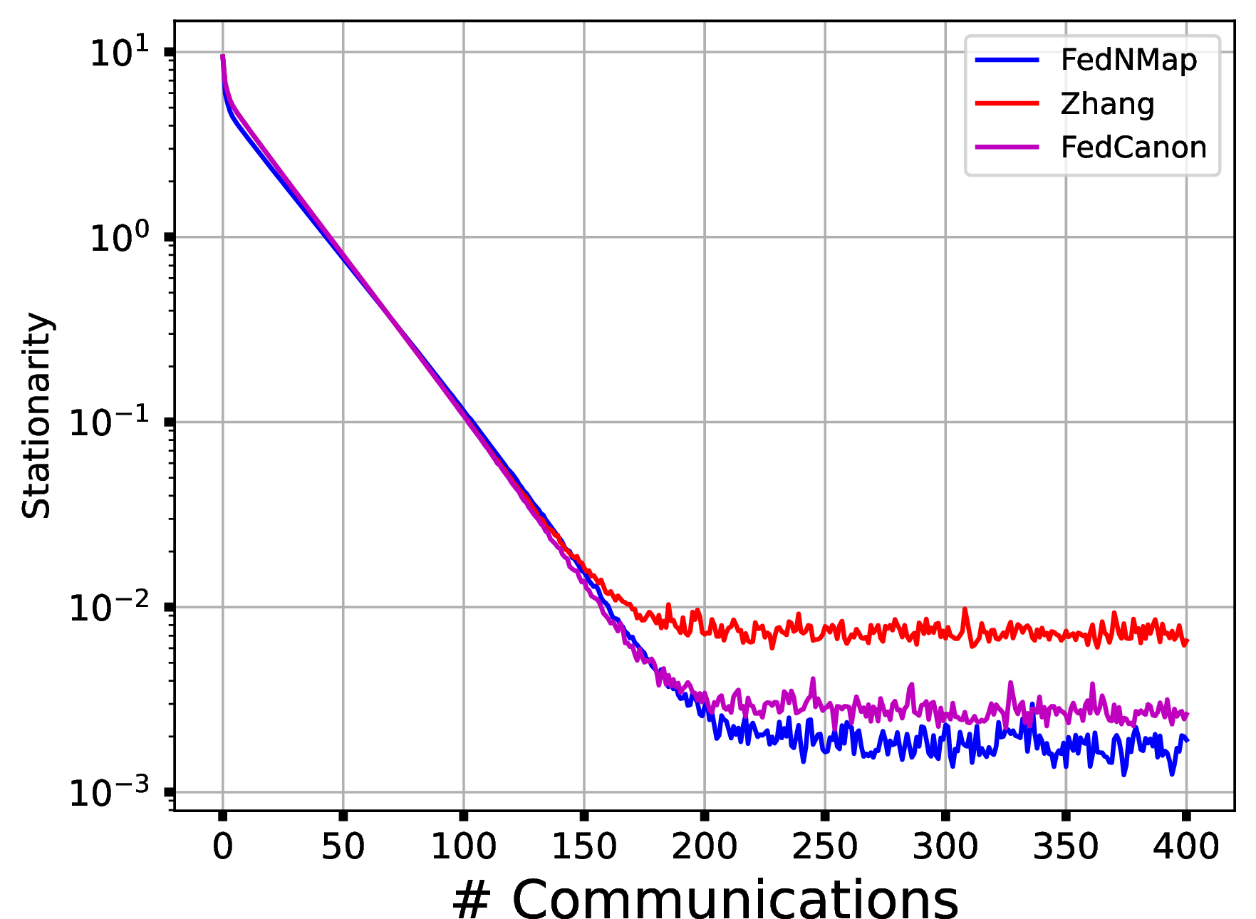
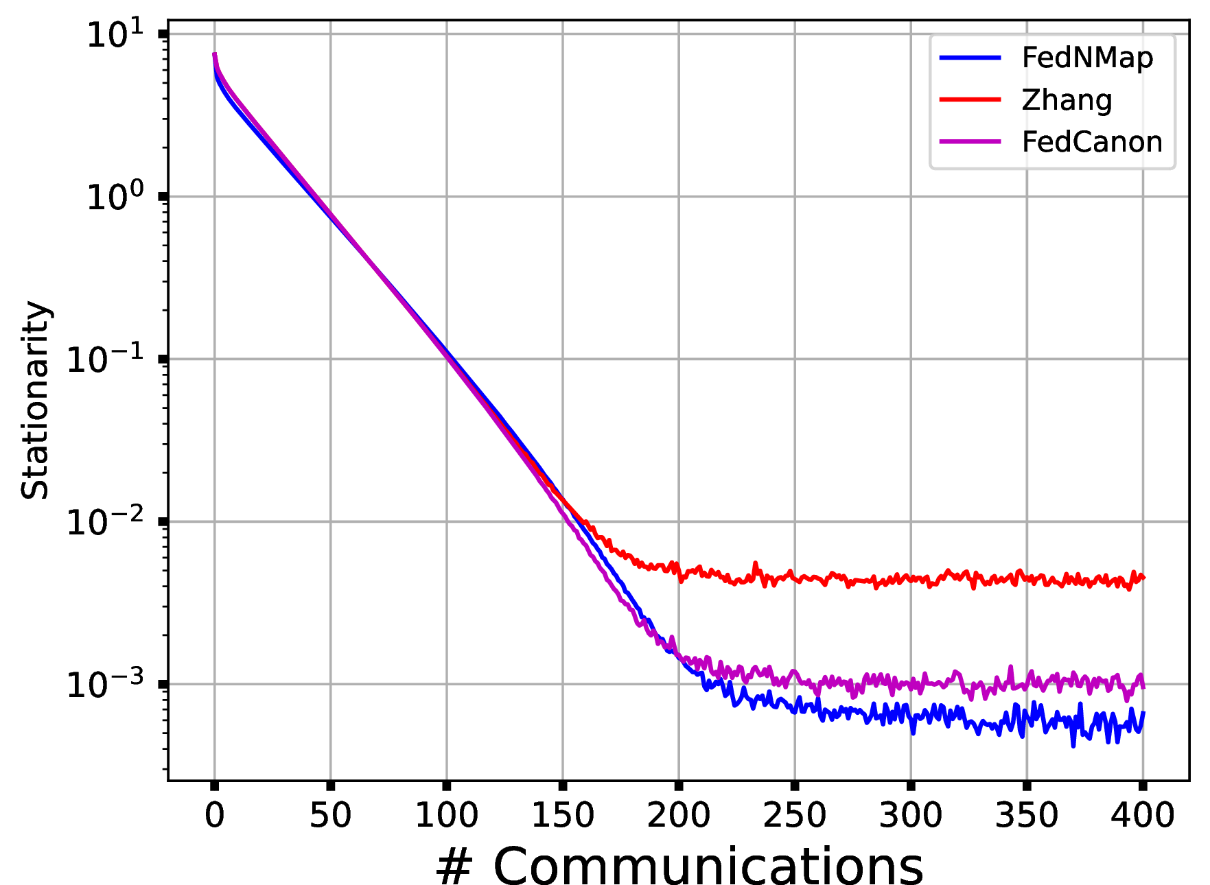
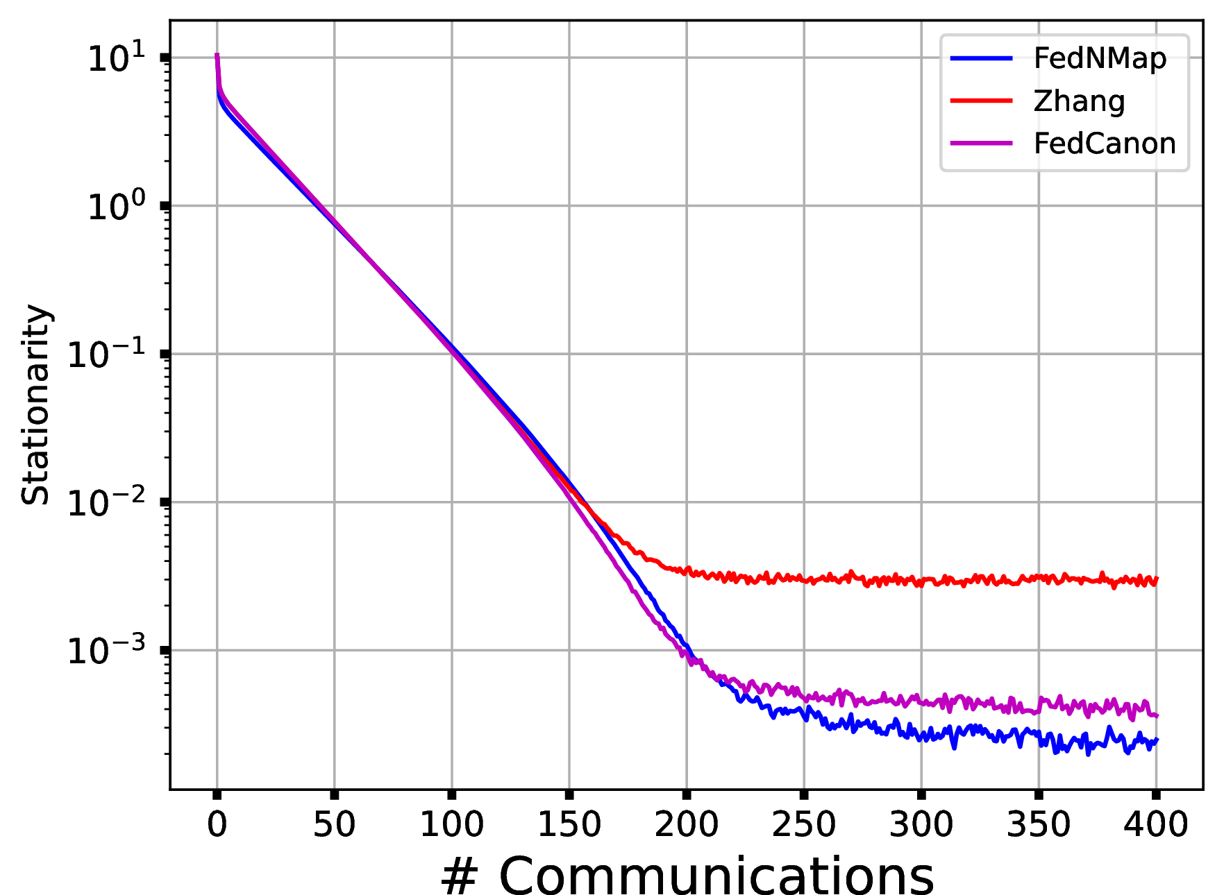
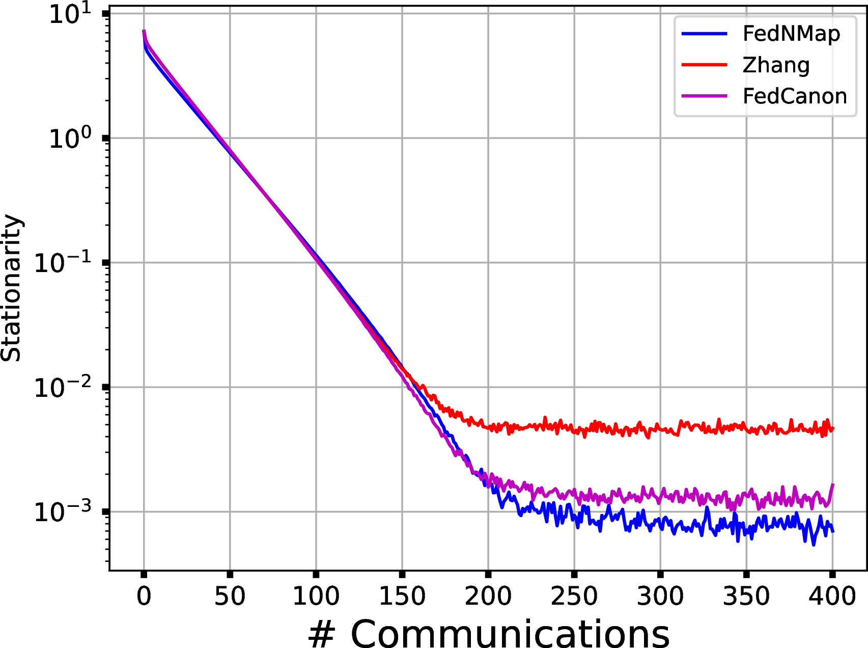
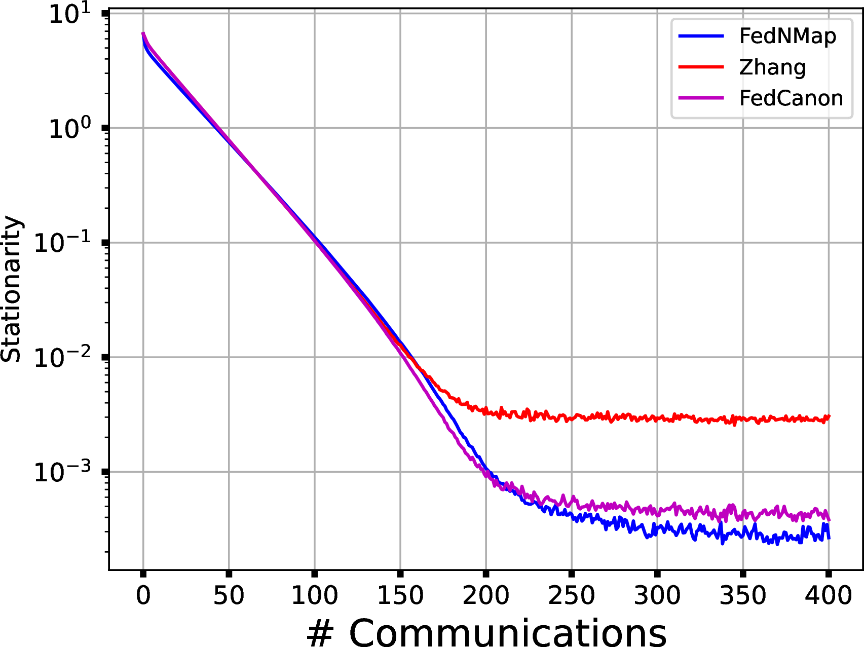
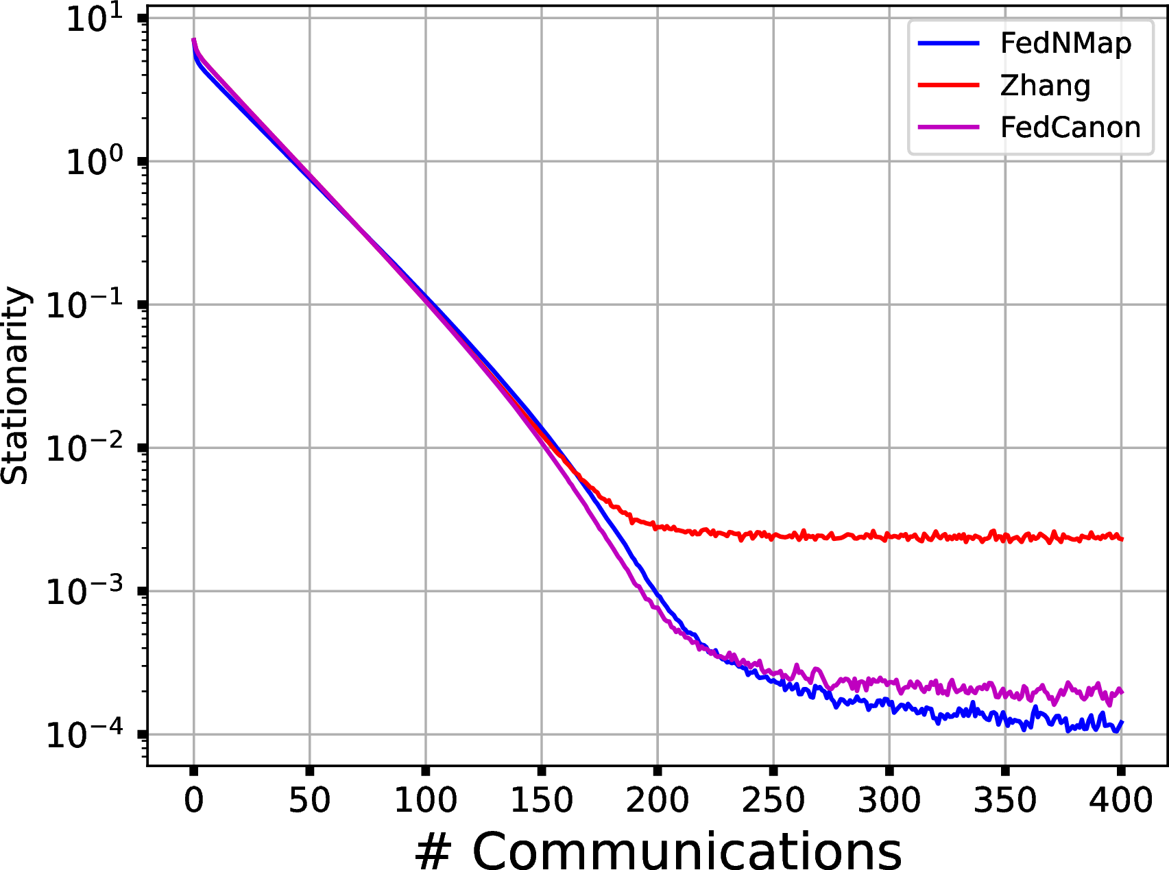
Figure 3: Comparison of FedNMap, Zhang [10], and FedCanon [11] for training a one-hidden-layer neural network with an elastic net regularizer on the MNIST data set. The stepsizes are set to \(\eta_a = 1/Q\) for local updates and \(\eta_s = 1\) for the outer loop across all methods. The parameter \(\gamma\) in FedNMapis set to \(4\)..
Figure 3 reports the stationarity measure \(\Vert \mathrm{F}^{\gamma}_{\mathrm{nat}}(x_t) \Vert^2\) against the number of communication rounds for varying numbers of clients \(n\) and local updates \(Q\). The stepsize rule \(\eta_a = 1/Q\) ensures that the effective stepsize \(\hat{\eta}= \eta_a\eta_s Q\) remains unchanged for different values of \(Q\). This makes the convergence speeds comparable, so lower stationarity values indicate better convergence. As shown in Figure 3, FedNMapconsistently achieves lower stationarity values than the other two methods across all tested configurations. Moreover, increasing the number of local updates from \(Q=10\) to \(Q=20\) (comparing Figures 3 (a) and 3 (d), Figures 3 (b) and 3 (e), or Figures 3 (c) and 3 (f)) improves convergence for a fixed \(n\). Similarly, increasing the number of clients from \(n=20\) to \(n=100\) (comparing Figures 3 (a)–3 (c) or Figures 3 (d)–3 (f)) improves convergence for a fixed \(Q\). These empirical observations are consistent with the dependence on \(n\) and \(Q\) predicted by Theorem 1 and further demonstrate the linear speedup for FedNMap.
To further examine the linear speedup of FedNMappredicted by Theorem 1, Figures 4 and 5 isolate the effects of the number of clients \(n\) and the number of local updates \(Q\), respectively.
Figure 4 (a) plots the stationarity measure against the number of communication rounds for different values of \(n\) with \(Q = 10\) fixed and a common effective stepsize \(\hat{\eta}= \eta_a\eta_s Q\). The results show that larger \(n\) leads to a smaller stationarity measure throughout the \(T\) communication rounds, which is consistent with the \(\mathcal{O}(1/\sqrt{nQT})\) convergence rate established in Theorem 1. Figure 4 (b) reports the final stationarity measure against \(\log n\). The steeper empirical slope (\(-1.436\)) compared to the theoretical prediction \((-0.5)\) suggests that the practical speedup with respect to \(n\) can be better in some problems.
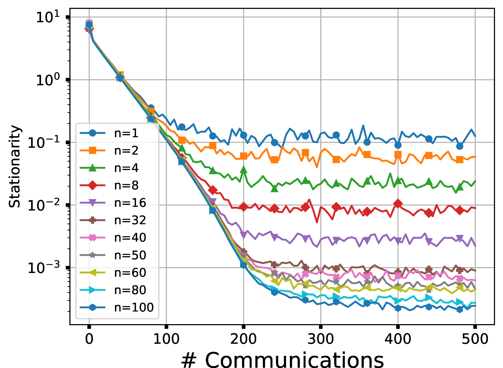
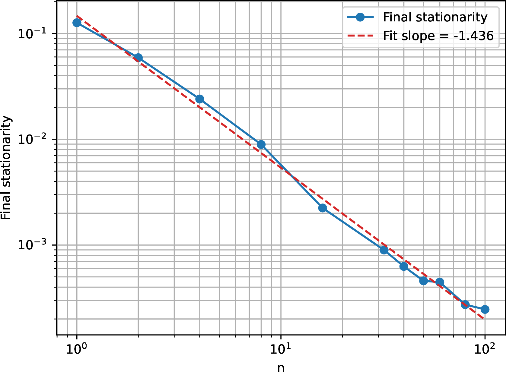
Figure 4: Empirical evaluation of the linear speedup of FedNMapwith respect to the number of clients \(n\) for fixed \(Q = 10\). The stepsizes are set to \(\eta_a = 0.1\) for local updates and \(\eta_s = 1\) for the outer loop across all \(n\). The parameter \(\gamma\) in FedNMapis set to \(4\)..
Figure 5 (a) plots the stationarity measure against the number of communication rounds for different values of \(Q\) with \(n = 30\) fixed and a common effective stepsize \(\hat{\eta}= \eta_a\eta_s Q\). The results show that larger \(Q\) leads to a smaller stationarity measure, which is consistent with the \(\mathcal{O}(1/\sqrt{nQT})\) convergence rate established in Theorem 1. Figure 5 (b) reports the final stationarity measure as a function of \(\log Q\). The steeper empirical slope (\(-1.181\)) compared to the theoretical prediction \((-0.5)\) suggests that the practical speedup with respect to \(Q\) can be better in some problems.
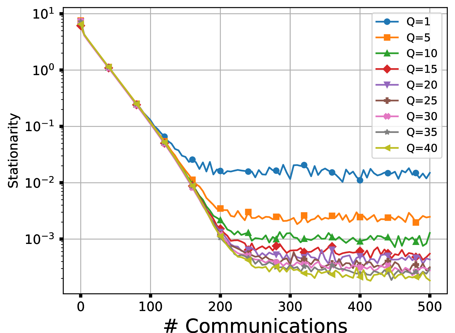
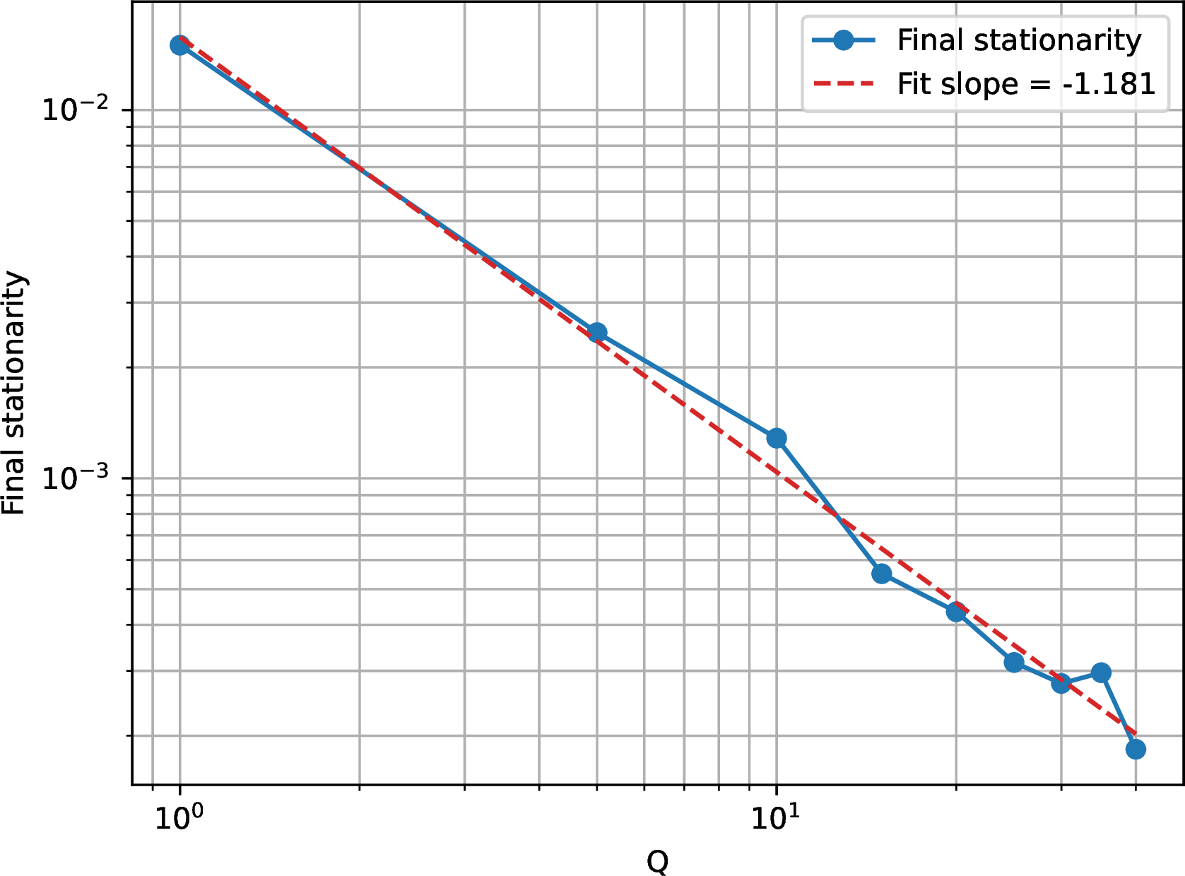
Figure 5: Empirical evaluation of the linear speedup property of FedNMapwith respect to the number of local updates \(Q\) with a fixed \(n = 30\). The stepsizes are set to \(\eta_a = 1/Q\) for local updates and \(\eta_s = 1\) for the outer loop across \(Q\). The parameter \(\gamma\) in FedNMapis set to \(4\)..
We also examine how the choice of \(\eta_a\) affects convergence behavior as \(Q\) varies. In Figure 6, we fix \(n = 30\) and \(\eta_s = 1\), vary \(Q\), and consider three local stepsize rules: \(\eta_a = 1/Q\), \(\eta_a = 1/\sqrt{Q}\), and \(\eta_a = 0.05\). In Figure 6 (a) (\(\eta_a = 1/Q\)), all curves share the same effective stepsize \(\hat{\eta}= \eta_a \eta_s Q\), and larger \(Q\) yields a smaller stationarity measure. In Figures 6 (b) (\(\eta_a = 1/\sqrt{Q}\)) and 6 (c) (\(\eta_a = 0.05\)), the effective stepsize \(\hat{\eta}\) increases with \(Q\), which leads to faster convergence for larger \(Q\) but a slightly higher yet comparable final stationarity measure. All the results demonstrate the linear speedup property of FedNMap.
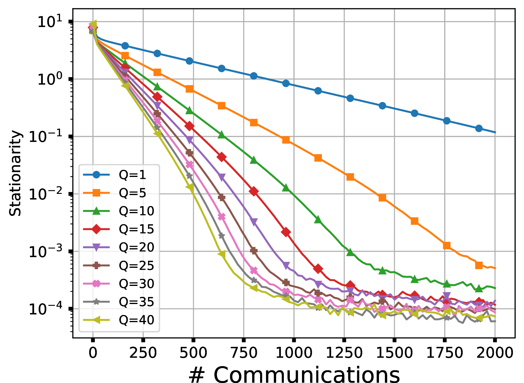
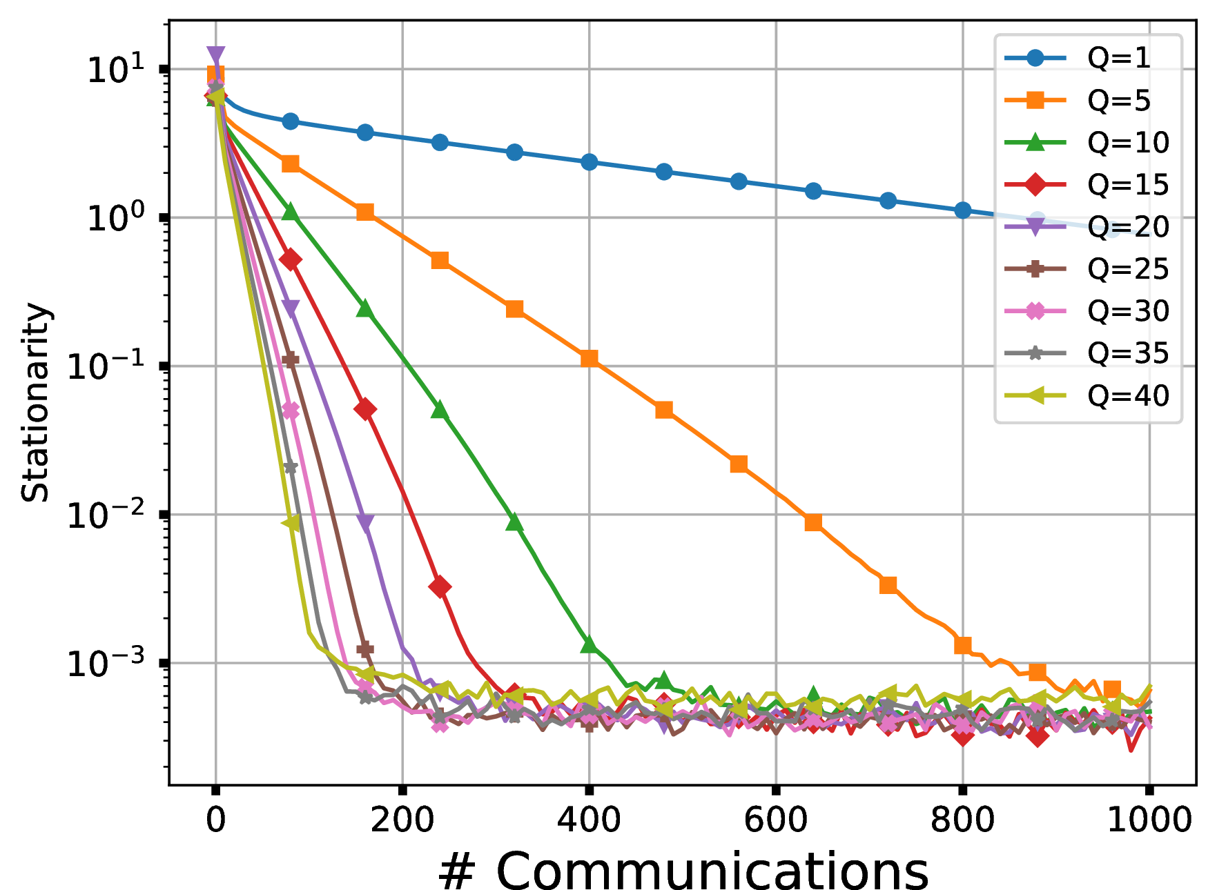
Figure 6: Empirical evaluation of FedNMapunder different choices of the local stepsize \(\eta_a\). We fix \(n=30\), \(\eta_s = 1\), and \(\gamma = 4\)..
5.2 MobileNetV3-Small↩︎
To assess the broader applicability of FedNMap, we conduct experiments on MobileNetV3-Small [30], a modern lightweight architecture with \(1.5\)M parameters designed for mobile devices. Since the model is intended for resource-constrained and low-latency scenarios, inducing sparsity is especially important. Accordingly, we add an \(\ell_1\)-norm regularizer to encourage sparse parameterization and use Hoyer’s sparsity \(s:= (\sqrt{p} - \Vert x \Vert_1/\Vert x \Vert_2)/(\sqrt{p}-1)\) for \(x\in\mathbb{R}^p\) to quantify the resulting sparsity level. In Figure 7, FedNMapconsistently achieves higher sparsity and lower training loss than Zhang and FedCanon.

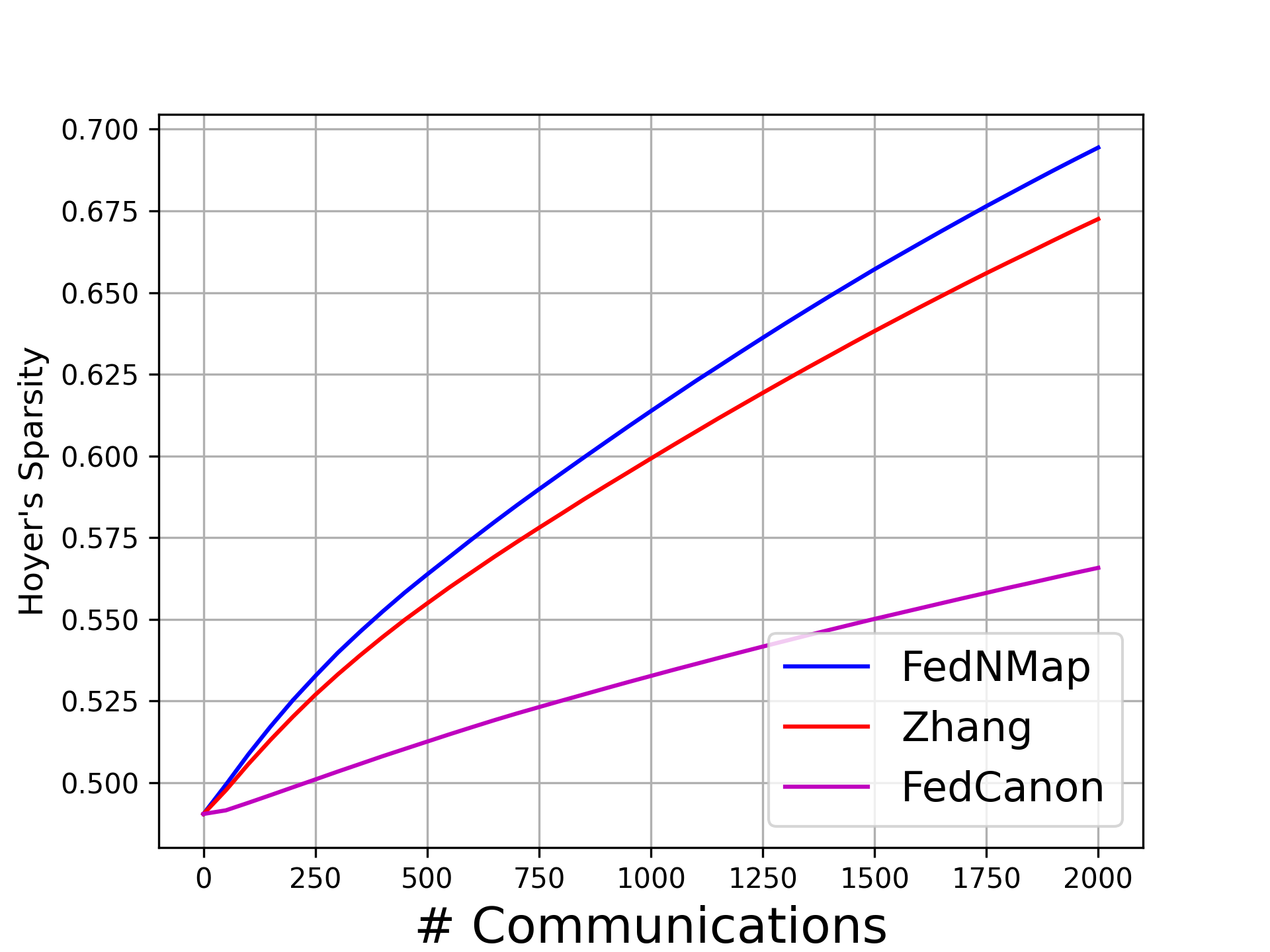

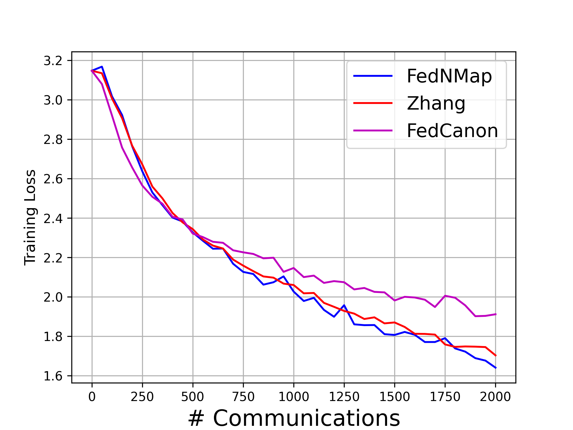
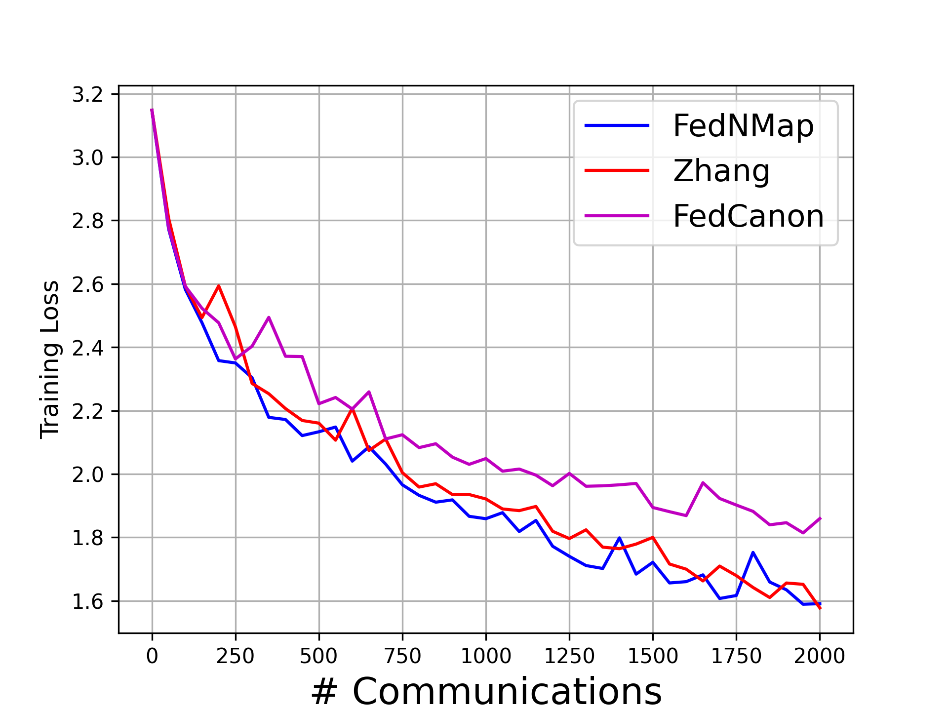
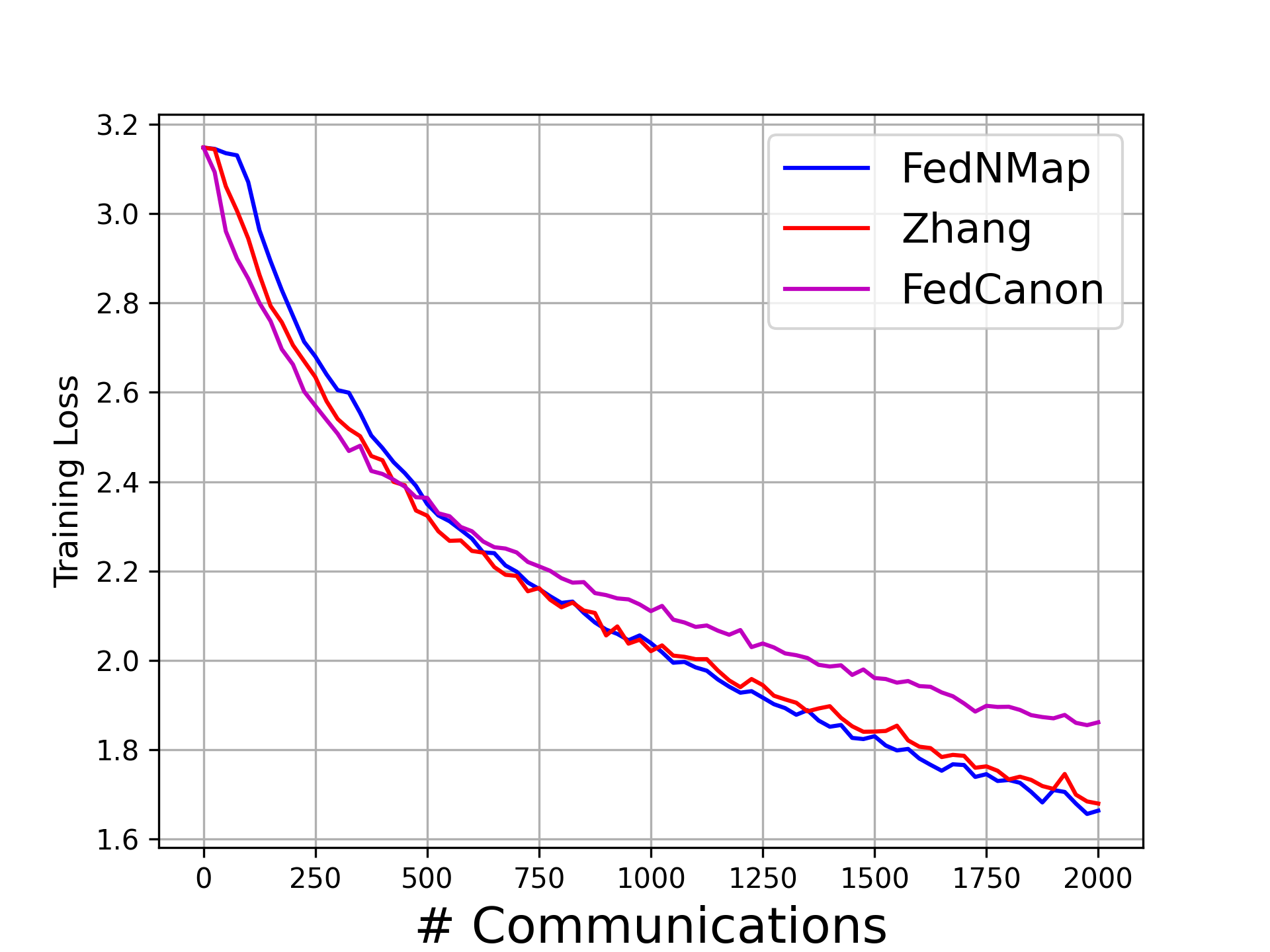
Figure 7: Comparison of FedNMap, Zhang, and FedCanon for training MobileNetV3-Small with an \(\ell_1\)-norm regularizer on the CIFAR-10. The stepsizes are set to \(\eta_a = 1 / Q\) and \(\eta_s=1\). The number of local updates is \(Q\in\{10,20\}\), the number of clients is \(n\in\{20,50\}\), and the parameter \(\gamma\) in FedNMapis set to \(2.5\)..
6 Conclusion↩︎
This paper introduced FedNMap, a novel algorithm for solving composite optimization problems in federated learning. By integrating a normal map-based update with a local correction mechanism, FedNMapeffectively addresses the challenges posed by a nonsmooth regularized term and data heterogeneity. We showed that linear speedup is achievable for composite FL with respect to both the number of clients and the number of local updates, covering both general nonconvex objectives and those that fulfill the PL condition. Numerical experiments validated our theoretical findings and demonstrated the effectiveness of the proposed algorithm.
7 Derivations for Related Methods↩︎
We present the derivations for comparison with existing methods below.
7.1 Method of Zhang et al. ↩︎
We restate the update rules in [10] and rewrite them in a form directly comparable to FedNMap. The method in [10] performs local updates as \[\label{eq:local95zhang} \begin{align} z_{i,t}^{\ell + 1} &= z_{i,t}^\ell - \eta_a\left(g_i(x_{i,t}^\ell;\xi_{i,t}^\ell) + c_{i,t}\right),\; x_{i,t}^{\ell + 1} = \mathrm{prox}_{(\ell + 1)\eta_a\varphi}(z_{i,t}^{\ell + 1}), \end{align}\tag{20}\] where \(z_{i,t}^0 = \mathrm{prox}_{\hat{\eta}}(z_t) = x_t\) and \(x_{i,t}^0 = x_t\) are received from the server. The server update is \[\label{eq:server95zhang} \begin{align} z_{t + 1} &= x_t + \eta_s\left(\frac{1}{n}\sum_{i=1}^nz_{i,t}^Q - x_t\right),\; x_{t + 1} = \mathrm{prox}_{\hat{\eta}\varphi}(z_{t + 1}). \end{align}\tag{21}\]
The correction term \(c_{i,t}\) is updated as \[\label{eq:cit95zhang} \begin{align} c_{i, t + 1} &= \frac{1}{\hat{\eta}}\left(x_t - z_{t + 1}\right) - \frac{1}{Q}\sum_{\ell=0}^{Q-1}g_i(x_{i,t}^\ell;\xi_{i,t}^\ell)\\ &= \frac{1}{nQ}\sum_{\ell=0}^{Q-1}\sum_{i=1}^ng_i(x_{i,t}^\ell;\xi_{i,t}^\ell) + \frac{1}{n}\sum_{i=1}^nc_{i,t} - \frac{1}{Q}\sum_{\ell=0}^{Q-1}g_i(x_{i,t}^\ell;\xi_{i,t}^\ell). \end{align}\tag{22}\]
By introducing \(y_{i,t}^{\rm (Z)} = (x_{t} - z_{i,t}^Q)/(\eta_a Q) = \sum_{\ell=0}^{Q-1}g_i(x_{i,t}^\ell;\xi_{i,t}^\ell)/Q + c_{i,t}\), we can rewrite the correction update and the server update in terms of \(y_{i,t}^{\rm (Z)}\) below. The correction update becomes \[\label{eq:cit95yit95zhang} \begin{align} c_{i,t + 1} &= \frac{1}{n}\sum_{i=1}^ny_{i,t}^{\rm (Z)} - y_{i,t}^{\rm (Z)} +c_{i,t}, \end{align}\tag{23}\] and the server updates as \[\label{eq:server95yit95zhang} \begin{align} z_{t + 1} &= x_t - \frac{Q\eta_s\eta_a}{n}\sum_{i=1}^ny_{i,t}^{\rm (Z)},\; x_{t + 1} = \mathrm{prox}_{\hat{\eta}}(z_{t + 1}). \end{align}\tag{24}\]
A derivation analogous to 9 demonstrates that \(y_{i,t}^{\rm (Z)}\) tracks the stochastic gradient as in 11 .
7.2 SCAFFOLD↩︎
For completeness, we also restate the update rules of SCAFFOLD [18] and express them in a form directly comparable to FedNMap.
The local updates of SCAFFOLD are given by \[\label{eq:local95scaffold} \begin{align} x_{i,t}^{\ell + 1} &= x_{i,t}^\ell - \eta_a\left[g_i(x_{i,t}^\ell;\xi_{i,t}^\ell) - c_{i,t} + c_t\right],\; x_{i,t}^0 = x_t,\\ c_{i,t+1} &= c_{i,t} - c_t + \frac{1}{\eta_a Q}\left(x_t - x_{i,t}^Q\right) = \frac{1}{Q}\sum_{\ell=0}^{Q-1}g_i(x_{i,t}^\ell;\xi_{i,t}^\ell). \end{align}\tag{25}\]
The server updates as \[\label{eq:server95scaffold} \begin{align} x_{t + 1} = x_t + \frac{\eta_s}{n}\sum_{i=1}^n\left(x_{i,t}^Q - x_t\right),\; c_{t + 1} = c_t + \frac{1}{n}\sum_{i=1}^n\left(c_{i,t + 1} - c_{i,t}\right). \end{align}\tag{26}\]
By introducing \(y_{i,t}^{\rm (S)} = (x_t - x_{i,t}^Q)/(\eta_a Q)\), we can rewrite 26 as \[\label{eq:server95yit95scaffold} \begin{align} x_{t + 1} = x_t - \frac{Q\eta_s\eta_a}{n}\sum_{i=1}^ny_{i,t}^{\rm (S)},\; c_{t + 1} = \frac{1}{n}\sum_{i=1}^ny_{i,t}^{\rm (S)}. \end{align}\tag{27}\]
Thus, \(y_{i,t}^{\rm (S)}\) admits the tracking recursion in 28 : \[\label{eq:yit95scaffold} \begin{align} y_{i,t + 1}^{\rm (S)} &= \frac{1}{Q}\sum_{\ell=0}^{Q-1}g_{i}(x_{i,t+1}^\ell;\xi_{i,t+1}^\ell) - c_{i,t + 1} + c_{t + 1}\\ &= \frac{1}{n}\sum_{i=1}^ny_{i,t}^{\rm (S)} + \frac{1}{Q}\sum_{\ell=0}^{Q-1}g_{i}(x_{i,t+1}^\ell;\xi_{i,t+1}^\ell) - \frac{1}{Q}\sum_{\ell=0}^{Q-1}g_{i}(x_{i,t}^\ell;\xi_{i,t}^\ell). \end{align}\tag{28}\]
8 Proofs of Preliminary Results↩︎
We begin with Lemma 5, which summarizes a nonexpansiveness property of the proximal mapping \(\mathrm{prox}_{\gamma\varphi}\left(\cdot\right)\) under Assumption 3. A proof can be found, for example, in [14].
Lemma 5. Let Assumption 3 hold. Set \(\gamma\in (0, \rho^{-1})\). We have for all \(w,v\in\mathbb{R}^p\) that
\(\left\langle w-v, \mathrm{prox}_{\gamma\varphi}\left(w\right) - \mathrm{prox}_{\gamma\varphi}\left(v\right) \right\rangle\geq (1-\gamma\rho)\left\Vert \mathrm{prox}_{\gamma\varphi}\left(w\right) - \mathrm{prox}_{\gamma\varphi}\left(v\right) \right\Vert^2\), and
\(\left\Vert w-v \right\Vert\geq (1-\gamma\rho)\left\Vert \mathrm{prox}_{\gamma\varphi}\left(w\right) - \mathrm{prox}_{\gamma\varphi}\left(v\right) \right\Vert\).
Lemma 6 then follows from Lemma 5 together with the definition of \(\mathrm{F}^{\gamma}_{\mathrm{nor}}(\cdot)\) in 2 . A proof can be found, for example, in [16], [24].
Lemma 6. Let Assumptions 2 and 3 hold. Set \(\gamma < 1/\rho\). The normal maps \(\mathrm{F}^{\gamma}_{\mathrm{nor}}(\cdot):\mathbb{R}^p\rightarrow\mathbb{R}^p\) and \({\mathrm{F}}^{\gamma}_{i,\mathrm{nor}}(\cdot): \mathbb{R}^p\rightarrow\mathbb{R}^p\) are \(L_{\mathrm{F}}\)-Lipschitz continuous, where \(L_{\mathrm{F}}:= (L + 2/\gamma)/(1 - \gamma\rho)\).
8.1 Proof of Lemma 1↩︎
Step I: Relating \(z_{t_1}\) and \(z_{t_2}\). Based on 6 and 7 , we have \[\label{eq:yit95z} y_{i,t} = \frac{1}{Q}\sum_{\ell=0}^{Q-1}\left[g_i(x_{i,t}^\ell;\xi_{i,t}^\ell) + \gamma^{-1}\left(z_{t} - x_{t}\right)\right] + c_{i,t}.\tag{29}\]
From 3 and the initialization \(c_{i,0} = 0\), we have \(\bar{c}_t = \bar{c}_0 = 0\) Accordingly, the server update can be written as the approximate normal map step \[\label{eq:ztp1} \begin{align} z_{t + 1} &= z_t - \frac{\hat{\eta}}{nQ}\sum_{i=1}^n \sum_{\ell=0}^{Q-1}\left[g_i(x_{i,t}^\ell;\xi_{i,t}^\ell) + \gamma^{-1}\left(z_{t} - x_{t}\right)\right]. \end{align}\tag{30}\]
Hence, we have for any \(t_1<t_2=t_1 + m\) that \[\label{eq:zt1t2} \begin{align} z_{t_2} &= z_{t_1} - \hat{\eta}m \mathrm{F}^{\gamma}_{\mathrm{nor}}(z_{t_1}) - \frac{\hat{\eta}}{nQ}\sum_{t=t_1}^{t_2-1}\sum_{i=1}^n \sum_{\ell=0}^{Q-1}\left[g_i(x_{i,t}^\ell;\xi_{i,t}^\ell) + \gamma^{-1}\left(z_{t} - x_{t}\right) - \mathrm{F}^{\gamma}_{\mathrm{nor}}(z_{t_1})\right]\\ &= z_{t_1} - \hat{\eta}m \mathrm{F}^{\gamma}_{\mathrm{nor}}(z_{t_1}) + e_{t_1:t_2}, \end{align}\tag{31}\] where \[\label{eq:et1t2} \begin{align} e_{t_1:t_2} &= - \frac{\hat{\eta}}{nQ}\sum_{t=t_1}^{t_2-1}\sum_{i=1}^n \sum_{\ell=0}^{Q-1}\left[g_i(x_{i,t}^\ell;\xi_{i,t}^\ell) + \gamma^{-1}\left(z_{t} - x_{t}\right) - \mathrm{F}^{\gamma}_{\mathrm{nor}}(z_{t_1})\right]\\ &= - \frac{\hat{\eta}}{nQ}\sum_{t=t_1}^{t_2-1}\sum_{i=1}^n \sum_{\ell=0}^{Q-1}\Delta_{i,t}^\ell - \frac{\hat{\eta}}{nQ}\sum_{t=t_1}^{t_2-1}\sum_{i=1}^n \sum_{\ell=0}^{Q-1}\left[\nabla f_i(x_{i,t}^\ell) - \nabla f_i(x_{t_1})\right]\\ &\quad + \frac{\hat{\eta}}{\gamma}\sum_{t=t_1}^{t_2-1} \left(z_{t_1} - z_t\right) - \frac{\hat{\eta}}{\gamma }\sum_{t=t_1}^{t_2-1} \left(x_{t_1} - x_t\right),\\ \Delta_{i,t}^\ell &= g_i(x_{i,t}^\ell;\xi_{i,t}^\ell) - \nabla f_i(x_{i,t}^\ell). \end{align}\tag{32}\]
Step II: Relating \(\psi(x_{t_1})\) and \(\psi(x_{t_2})\). Due to Assumption 3 that \(\varphi\) is \(\rho\)-weakly convex, we have for any \(x, x'\in\mathrm{dom}(\varphi)\) and any \(v\in\partial\varphi(x')\) that \[\label{eq:wcvx0} \varphi(x)\geq \varphi(x') + \left\langle v, x - x' \right\rangle - \frac{\rho}{2}\left\Vert x - x' \right\Vert^2.\tag{33}\]
Noting \(x_{t_2} = \mathrm{prox}_{\gamma\varphi}\left(z_{t_2}\right)\), it follows from the second prox theorem [27] that \(\gamma^{-1}(z_{t_2} - x_{t_2})\in\partial \varphi(x_{t_2})\). Therefore, setting \(x' = x_{t_2}\), \(x = x_{t_1}\), and \(v = \gamma^{-1}(z_{t_2} - x_{t_2})\) in 33 leads to \[\label{eq:phi95t1t2} \begin{align} \varphi(x_{t_2}) &\leq \varphi(x_{t_1}) - \left\langle \gamma^{-1}(z_{t_2} - x_{t_2}), x_{t_1} - x_{t_2} \right\rangle + \frac{\rho}{2}\left\Vert x_{t_2} - x_{t_1} \right\Vert^2. \end{align}\tag{34}\]
Applying the descent lemma to \(f\) yields \[\label{eq:f95t1t2} \begin{align} f(x_{t_2}) &\leq f(x_{t_1}) + \left\langle \nabla f(x_{t_1}), x_{t_2} - x_{t_1} \right\rangle + \frac{L}{2}\left\Vert x_{t_2} - x_{t_1} \right\Vert^2\\ &= f(x_{t_1}) + \left\langle \mathrm{F}^{\gamma}_{\mathrm{nor}}(z_{t_1}) - \gamma^{-1}(z_{t_1} - x_{t_1}), x_{t_2} - x_{t_1} \right\rangle + \frac{L}{2}\left\Vert x_{t_2} - x_{t_1} \right\Vert^2. \end{align}\tag{35}\]
Combining 34 and 35 leads to \[\label{eq:psi95t1t2} \begin{align} \psi(x_{t_2}) &\leq \psi(x_{t_1}) + \left\langle \mathrm{F}^{\gamma}_{\mathrm{nor}}(z_{t_1}), x_{t_2} - x_{t_1} \right\rangle + \left(\frac{L + \rho}{2} - \frac{1}{\gamma}\right)\left\Vert x_{t_2} - x_{t_1} \right\Vert^2\\ &\quad + \left\langle \gamma^{-1}(z_{t_2} - z_{t_1}), x_{t_2} - x_{t_1} \right\rangle. \end{align}\tag{36}\]
Step III: Relating \(\Vert \mathrm{F}^{\gamma}_{\mathrm{nor}}(z_{t_1}) \Vert^2\) and \(\Vert \mathrm{F}^{\gamma}_{\mathrm{nor}}(z_{t_2}) \Vert^2\). According to 31 , we have \(\mathrm{F}^{\gamma}_{\mathrm{nor}}(z_{t_2})= (1 - {\hat{\eta}m}/{\gamma})\mathrm{F}^{\gamma}_{\mathrm{nor}}(z_{t_1}) + \nabla f(x_{t_2}) - \nabla f(x_{t_1}) - \gamma^{-1}(x_{t_2} - x_{t_1}) + \gamma^{-1}e_{t_1:t_2}.\) Hence, \[\label{eq:Fnor95t1t295norm} \begin{align} &\left\Vert \mathrm{F}^{\gamma}_{\mathrm{nor}}(z_{t_2}) \right\Vert^2 = \left(1 - \frac{\hat{\eta}m}{\gamma}\right)^2\left\Vert \mathrm{F}^{\gamma}_{\mathrm{nor}}(z_{t_1}) \right\Vert^2 + \left\Vert \nabla f(x_{t_2}) - \nabla f(x_{t_1}) \right\Vert^2 + \frac{1}{\gamma^2}\left\Vert x_{t_2} - x_{t_1} \right\Vert^2 \\ &\quad + \frac{1}{\gamma^2}\left\Vert e_{t_1:t_2} \right\Vert^2 + 2\left(1 - \frac{\hat{\eta}m}{\gamma}\right)\left\langle \mathrm{F}^{\gamma}_{\mathrm{nor}}(z_{t_1}), \nabla f(x_{t_2}) - \nabla f(x_{t_1}) - \gamma^{-1}(x_{t_2} - x_{t_1}) + \gamma^{-1}e_{t_1:t_2} \right\rangle\\ &\quad + \frac{2}{\gamma}\left\langle \nabla f(x_{t_2}) - \nabla f(x_{t_1}) - \gamma^{-1}(x_{t_2} - x_{t_1}), e_{t_1:t_2} \right\rangle - \frac{2}{\gamma}\left\langle \nabla f(x_{t_2}) - \nabla f(x_{t_1}), x_{t_2} - x_{t_1} \right\rangle\\ &\leq \left(1 - \frac{\hat{\eta}m}{\gamma}\right)^2\left\Vert \mathrm{F}^{\gamma}_{\mathrm{nor}}(z_{t_1}) \right\Vert^2 + \left(L + \frac{1}{\gamma}\right)^2 \left\Vert x_{t_2} - x_{t_1} \right\Vert^2 + \frac{1}{\gamma^2}\left\Vert e_{t_1:t_2} \right\Vert^2\\ &\quad + 2\left(1 - \frac{\hat{\eta}m}{\gamma}\right)\left\langle \mathrm{F}^{\gamma}_{\mathrm{nor}}(z_{t_1}), \nabla f(x_{t_2}) - \nabla f(x_{t_1}) - \gamma^{-1}(x_{t_2} - x_{t_1}) + \gamma^{-1}e_{t_1:t_2} \right\rangle\\ &\quad + \frac{2}{\gamma^2}\left\langle \gamma\left[\nabla f(x_{t_2}) - \nabla f(x_{t_1})\right] - (x_{t_2} - x_{t_1}), e_{t_1:t_2} \right\rangle, \end{align}\tag{37}\] where we applied the Cauchy-Schwarz inequality and invoked the \(L\)-smoothness of \(f\) in the last inequality.
Step IV: Relating \(\mathcal{H}_{t_1}\) and \(\mathcal{H}_{t_2}\). Substituting 37 and 36 into 17 and rearranging the terms yields \[\label{eq:cH95can95s1} \begin{align} \mathcal{H}_{t_2} &\leq \mathcal{H}_{t_1} + \left[\frac{L + \rho}{2} - \frac{1}{\gamma} + \frac{\gamma \mathcal{C}_0}{2}\left(L + \frac{1}{\gamma}\right)^2\right]\left\Vert x_{t_2} - x_{t_1} \right\Vert^2 + \frac{\mathcal{C}_0}{2\gamma}\left\Vert e_{t_1:t_2} \right\Vert^2\\ &\quad + \left\langle \mathrm{F}^{\gamma}_{\mathrm{nor}}(z_{t_1}) - \mathcal{C}_0\left(1-\frac{\hat{\eta}m}{\gamma}\right)\mathrm{F}^{\gamma}_{\mathrm{nor}}(z_{t_1}) + \frac{z_{t_2}-z_{t_1}}{\gamma} - \frac{\mathcal{C}_0 e_{t_1:t_2}}{\gamma}, x_{t_2} - x_{t_1} \right\rangle\\ &\quad + \mathcal{C}_0\left(1 - \frac{\hat{\eta}m}{\gamma}\right)\left\langle \mathrm{F}^{\gamma}_{\mathrm{nor}}(z_{t_1}), \gamma\left[\nabla f(x_{t_2}) - \nabla f(x_{t_1})\right] + e_{t_1:t_2} \right\rangle\\ &\quad + \frac{\mathcal{C}_0}{\gamma}\left\langle \gamma\left[\nabla f(x_{t_2}) - \nabla f(x_{t_1})\right], e_{t_1:t_2} \right\rangle - \frac{\mathcal{C}_0 \hat{\eta}m}{2}\left(2- \frac{\hat{\eta}m}{\gamma}\right)\left\Vert \mathrm{F}^{\gamma}_{\mathrm{nor}}(z_{t_1}) \right\Vert^2. \end{align}\tag{38}\]
According to 31 , we have \(e_{t_1:t_2} - \hat{\eta}m \mathrm{F}^{\gamma}_{\mathrm{nor}}(z_{t_1}) = z_{t_2} - z_{t_1}\) and \(\mathrm{F}^{\gamma}_{\mathrm{nor}}(z_{t_1}) = (z_{t_1} - z_{t_2} + e_{t_1:t_2})/(\hat{\eta}m)\). Then, \[\label{eq:cH95inner1} \begin{align} &\left\langle \mathrm{F}^{\gamma}_{\mathrm{nor}}(z_{t_1}) - \mathcal{C}_0\left(1-\frac{\hat{\eta}m}{\gamma}\right)\mathrm{F}^{\gamma}_{\mathrm{nor}}(z_{t_1}) + \frac{z_{t_2}-z_{t_1}}{\gamma} - \frac{\mathcal{C}_0 e_{t_1:t_2}}{\gamma}, x_{t_2} - x_{t_1} \right\rangle\\ &= \left\langle (1-\mathcal{C}_0)\left(1-\frac{\hat{\eta}m}{\gamma}\right)\mathrm{F}^{\gamma}_{\mathrm{nor}}(z_{t_1})+\frac{1-\mathcal{C}_0}{\gamma}e_{t_1:t_2}, x_{t_2} - x_{t_1} \right\rangle\\ &= \frac{1-\mathcal{C}_0}{\hat{\eta}m}\left\langle e_{t_1:t_2}, x_{t_2} - x_{t_1} \right\rangle - \left(1-\mathcal{C}_0\right)\left(\frac{1}{\hat{\eta}m}-\frac{1}{\gamma}\right)\left\langle z_{t_2} - z_{t_1}, x_{t_2} - x_{t_1} \right\rangle\\ &\leq \left[\frac{1-\mathcal{C}_0}{4\hat{\eta}m} - \left(1-\mathcal{C}_0\right)\left(\frac{1}{\hat{\eta}m} - \frac{1}{\gamma}\right)\left(1-\gamma \rho\right)\right]\left\Vert x_{t_2} - x_{t_1} \right\Vert^2 + \frac{1-\mathcal{C}_0}{\hat{\eta}m}\left\Vert e_{t_1:t_2} \right\Vert^2, \end{align}\tag{39}\] where we applied Lemma 5 by noting \(x_t = \mathrm{prox}_{\gamma\varphi}(z_t)\) and setting \(0<\mathcal{C}_0<1\) and \(\hat{\eta}m < \gamma\): \[\begin{align} - \left(1-\mathcal{C}_0\right)\left(\frac{1}{\hat{\eta}m}-\frac{1}{\gamma}\right)\left\langle z_{t_2} - z_{t_1}, x_{t_2} - x_{t_1} \right\rangle &\leq (1 - \gamma \rho)\left(1-\mathcal{C}_0\right)\left(\frac{1}{\hat{\eta}m}-\frac{1}{\gamma}\right)\left\Vert x_{t_2} - x_{t_1} \right\Vert^2, \end{align}\] and Young’s inequality: \[\begin{align} \left\langle e_{t_1:t_2}, x_{t_2} - x_{t_1} \right\rangle &\leq \frac{1}{4}\left\Vert x_{t_2} - x_{t_1} \right\Vert^2 + \left\Vert e_{t_1:t_2} \right\Vert^2. \end{align}\]
For the remaining inner products in 38 , it follows from Young’s inequality that \[\label{eq:cH95inners} \begin{align} \left\langle \mathrm{F}^{\gamma}_{\mathrm{nor}}(z_{t_1}), \gamma\left[\nabla f(x_{t_2}) - \nabla f(x_{t_1})\right] + e_{t_1:t_2} \right\rangle &\leq \frac{\hat{\eta}m}{2}\left\Vert \mathrm{F}^{\gamma}_{\mathrm{nor}}(z_{t_1}) \right\Vert^2 + \frac{\gamma^2 L^2 \Vert x_{t_1} - x_{t_2} \Vert^2 + \Vert e_{t_1:t_2} \Vert^2}{\hat{\eta}m} \\ \frac{\mathcal{C}_0}{\gamma}\left\langle \gamma\left[\nabla f(x_{t_2}) - \nabla f(x_{t_1})\right], e_{t_1:t_2} \right\rangle&\leq \frac{\mathcal{C}_0 L}{2}\left\Vert x_{t_1} - x_{t_2} \right\Vert^2 + \frac{\mathcal{C}_0 L}{2}\left\Vert e_{t_1:t_2} \right\Vert^2. \end{align}\tag{40}\]
Substituting 39 and 40 into 38 leads to \[\label{eq:cH95can95s2} \begin{align} &\mathcal{H}_{t_2} \leq \mathcal{H}_{t_1} - \frac{\mathcal{C}_0\hat{\eta}m}{2}\left[2 - \frac{\hat{\eta}m}{\gamma} - \left(1 - \frac{\hat{\eta}m}{\gamma}\right)\right]\left\Vert \mathrm{F}^{\gamma}_{\mathrm{nor}}(z_{t_1}) \right\Vert^2 + \mathtt{C}_1 \left\Vert x_{t_1} - x_{t_2} \right\Vert^2\\ &\quad + \left[\frac{\mathcal{C}_0}{2\gamma} + \frac{1-\mathcal{C}_0}{\hat{\eta}m} + \frac{\mathcal{C}_0(1-\hat{\eta}m /\gamma)}{\hat{\eta}m} + \frac{\mathcal{C}_0 L}{2}\right]\left\Vert e_{t_1:t_2} \right\Vert^2, \end{align}\tag{41}\] where \[\begin{align} \mathtt{C}_1&:= \left[\frac{L + \rho}{2} - \frac{1}{\gamma} + \frac{\gamma \mathcal{C}_0}{2}\left(L + \frac{1}{\gamma}\right)^2\right] + \left[\frac{1-\mathcal{C}_0}{4\hat{\eta}m} - \left(1-\mathcal{C}_0\right)\left(\frac{1}{\hat{\eta}m} - \frac{1}{\gamma}\right)\left(1-\gamma \rho\right)\right] \\ &\quad + \frac{\mathcal{C}_0\gamma^2 L^2}{\hat{\eta}m}\left(1 - \frac{\hat{\eta}m}{\gamma}\right) + \frac{\mathcal{C}_0 L}{2}\\ &= -\frac{3-4\gamma\rho}{4\hat{\eta}m } + \frac{\mathcal{C}_0\left(3 - 4\gamma\rho + 4\gamma^2 L^2\right)}{4\hat{\eta}m} + \mathcal{C}_0\left(\rho - \frac{1}{2\gamma} + \frac{3L}{2} - \frac{\gamma L^2}{2}\right) + \frac{L-\rho}{2}. \end{align}\]
Based on the definition of \(\mathcal{C}_0\) in 17 and \(\gamma\leq 1/[5(\rho + L)]\), we have \(\mathcal{C}_0 < 1/2\) and \(\mathcal{C}_0[\rho - {1}/(2\gamma) + 1.5L - 0.5\gamma L^2] + 0.5(L-\rho) < 0.\) Therefore, \[\label{eq:cH} \begin{align} \mathcal{H}_{t_2} &\leq \mathcal{H}_{t_1} - \frac{\mathcal{C}_0 \hat{\eta}m}{2}\left\Vert \mathrm{F}^{\gamma}_{\mathrm{nor}}(z_{t_1}) \right\Vert^2 - \frac{1}{8\hat{\eta}m}\left\Vert x_{t_1} - x_{t_2} \right\Vert^2 + \frac{1}{\hat{\eta}m}\left\Vert e_{t_1:t_2} \right\Vert^2. \end{align}\tag{42}\]
Step V: Upper bounding \(\mathbb{E}[\Vert e_{t_1:t_2} \Vert^2|\mathcal{F}_{t_1}]\). We now bound \(\mathbb{E}[\Vert e_{t_1:t_2} \Vert^2|\mathcal{F}_{t_1}]\). We start with any \((t_1+1)\leq t\leq t_2\). Let \[\label{eq:et1t} \begin{align} e_{t_1:t}&:= - \frac{\hat{\eta}}{nQ}\sum_{r=t_1}^{t-1}\sum_{\ell=0}^{Q-1}\sum_{i=1}^n\left[g_i(x_{i,r}^\ell;\xi_{i,r}^\ell) + \gamma^{-1}\left(z_r - x_r\right) - \mathrm{F}^{\gamma}_{\mathrm{nor}}(z_{t_1})\right],\; t_1+1\leq t\leq t_2. \end{align}\tag{43}\]
It follows from 30 that \[\label{eq:zt95zt1} \begin{align} z_t &= z_{t_1} - \hat{\eta}(t - t_1) \mathrm{F}^{\gamma}_{\mathrm{nor}}(z_{t_1}) + e_{t_1:t},\; t_1 + 1 \leq t \leq t_2. \end{align}\tag{44}\]
Noting that \(\Delta_{i,t}^\ell = g_i(x_{i,t}^\ell;\xi_{i,t}^\ell) - \nabla f_i(x_{i,t}^\ell)\), we obtain the following relation for \(e_{t_1:t}\): \[\label{eq:et1t95split} \begin{align} e_{t_1:t} &= - \frac{\hat{\eta}}{nQ}\sum_{r=t_1}^{t-1} \sum_{\ell=0}^{Q-1} \sum_{i=1}^n\Delta_{i,r}^\ell - \frac{\hat{\eta}}{nQ}\sum_{r=t_1}^{t-1} \sum_{\ell=0}^{Q-1}\sum_{i=1}^n\left[\nabla f_i(x_{i,r}^\ell) - \nabla f_i(x_{t_1})\right]\\ &\quad + \frac{\hat{\eta}}{\gamma }\sum_{r=t_1}^{t-1} \left(z_{t_1} - z_{r}\right) - \frac{\hat{\eta}}{\gamma }\sum_{r=t_1}^{t-1} \left(x_{t_1} - x_{r}\right),\; t_1 + 1 \leq t \leq t_2. \end{align}\tag{45}\]
Taking the squared norm and conditional expectation on both sides of 45 and invoking Assumption 2 yields \[\label{eq:et1t95norm} \begin{align} &\frac{1}{4}\mathbb{E}\left[\left\Vert e_{t_1:t} \right\Vert^2\middle|\mathcal{F}_{t_1}\right]\leq \frac{\hat{\eta}^2 L^2 (t-t_1)}{nQ}\sum_{r=t_1}^{t-1} \sum_{\ell=0}^{Q-1}\sum_{i=1}^n\mathbb{E}\left[\left\Vert \mathrm{prox}_{\gamma\varphi}\left(z_{i,r}^\ell\right) - \mathrm{prox}_{\gamma\varphi}\left(z_{t_1}\right) \right\Vert^2\middle|\mathcal{F}_{t_1}\right] \\ &\quad + \frac{\hat{\eta}^2 (t-t_1)\sigma^2}{nQ} + \frac{\hat{\eta}^2 (t-t_1)}{ \gamma^2} \sum_{r=t_1}^{t-1} \mathbb{E}\left[\left\Vert z_{t_1} - z_{r} \right\Vert^2\middle|\mathcal{F}_{t_1}\right]\\ &\quad + \frac{\hat{\eta}^2(t-t_1)}{\gamma^2}\sum_{r=t_1}^{t-1}\mathbb{E}\left[\left\Vert \mathrm{prox}_{\gamma\varphi}\left(z_{t_1}\right) - \mathrm{prox}_{\gamma\varphi}\left(z_r\right) \right\Vert^2\middle|\mathcal{F}_{t_1}\right]\\ &\leq \frac{\hat{\eta}^2 (t-t_1)\sigma^2}{nQ} + \frac{\hat{\eta}^2 L^2 (t-t_1)}{nQ(1-\gamma\rho)^2 } \sum_{r=t_1}^{t-1} \sum_{\ell=0}^{Q-1}\sum_{i=1}^n \mathbb{E}\left[\left\Vert z_{t_1} - z_{i,r}^\ell \right\Vert^2\middle|\mathcal{F}_{t_1}\right]\\ &\quad + \frac{2\hat{\eta}^2 (t-t_1)}{\gamma^2(1-\gamma\rho)^2}\sum_{r=t_1}^{t-1}\mathbb{E}\left[\left\Vert z_{t_1} - z_r \right\Vert^2\middle|\mathcal{F}_{t_1}\right],\; t_1 + 1 \leq t \leq t_2, \end{align}\tag{46}\] where we invoked Lemma 5 in the last inequality. We next bound the last summation in 46 . It follows from 44 that \[\label{eq:zr95zt1} \begin{align} &\mathbb{E}\left[\left\Vert z_t - z_{t_1} \right\Vert^2\middle|\mathcal{F}_{t_1}\right] \leq 2\hat{\eta}^2 (t - t_1)^2\left\Vert \mathrm{F}^{\gamma}_{\mathrm{nor}}(z_{t_1}) \right\Vert^2 + 2\mathbb{E}\left[\left\Vert e_{t_1:t} \right\Vert^2\middle|\mathcal{F}_{t_1}\right]\\ &\leq 2\hat{\eta}^2 (t - t_1)^2\left\Vert \mathrm{F}^{\gamma}_{\mathrm{nor}}(z_{t_1}) \right\Vert^2 + \frac{8\hat{\eta}^2 (t-t_1)\sigma^2}{nQ} + \frac{16\hat{\eta}^2 (t-t_1)}{\gamma^2(1-\gamma\rho)^2}\sum_{r=t_1}^{t-1}\mathbb{E}\left[\left\Vert z_{t_1} - z_r \right\Vert^2\middle|\mathcal{F}_{t_1}\right] \\ &\quad + \frac{8\hat{\eta}^2 L^2 (t-t_1)}{nQ(1-\gamma\rho)^2 } \sum_{r=t_1}^{t-1} \sum_{\ell=0}^{Q-1}\sum_{i=1}^n \mathbb{E}\left[\left\Vert z_{t_1} - z_{i,r}^\ell \right\Vert^2\middle|\mathcal{F}_{t_1}\right] ,\; \forall t_1 + 1 \leq t \leq t_2. \end{align}\tag{47}\]
By convention, an empty sum is zero. Then 47 also holds for \(t = t_1\). Summing \(t = t_1\), \(t_1 + 1\), \(t_1 + 2\), \(\ldots\), \(t_2\) on both sides of 47 and noting \(t_2 - t_1 = m\) yields \[\label{eq:sum95zt95zt1} \begin{align} &\left[1 - \frac{8\hat{\eta}^2 m^2}{\gamma^2(1-\gamma\rho)^2}\right]\sum_{t=t_1}^{t_2}\mathbb{E}\left[\left\Vert z_t - z_{t_1} \right\Vert^2\middle|\mathcal{F}_{t_1}\right] \leq \hat{\eta}^2 m^3 \left\Vert \mathrm{F}^{\gamma}_{\mathrm{nor}}(z_{t_1}) \right\Vert^2 + \frac{4\hat{\eta}^2 m^2\sigma^2}{nQ} \\ &\quad + \frac{4\hat{\eta}^2 L^2 m^2}{nQ(1-\gamma\rho)^2 } \sum_{t=t_1}^{t_2-1} \sum_{\ell=0}^{Q-1}\sum_{i=1}^n \mathbb{E}\left[\left\Vert z_{t_1} - z_{i,t}^\ell \right\Vert^2\middle|\mathcal{F}_{t_1}\right]. \end{align}\tag{48}\]
Letting \(\hat{\eta}\leq (1-\gamma\rho)\gamma/(4m)\) yields \[\label{eq:sum95zt95zt195ub} \begin{align} &\sum_{t=t_1}^{t_2-1}\mathbb{E}\left[\left\Vert z_t - z_{t_1} \right\Vert^2\middle|\mathcal{F}_{t_1}\right] \leq \sum_{t=t_1}^{t_2}\mathbb{E}\left[\left\Vert z_t - z_{t_1} \right\Vert^2\middle|\mathcal{F}_{t_1}\right] \leq 2\hat{\eta}^2 m^3 \left\Vert \mathrm{F}^{\gamma}_{\mathrm{nor}}(z_{t_1}) \right\Vert^2 + \frac{8\hat{\eta}^2 m^2\sigma^2}{nQ} \\ &\quad + \frac{8\hat{\eta}^2 L^2 m^2}{nQ(1-\gamma\rho)^2 } \sum_{t=t_1}^{t_2-1} \sum_{\ell=0}^{Q-1}\sum_{i=1}^n \mathbb{E}\left[\left\Vert z_{t_1} - z_{i,t}^\ell \right\Vert^2\middle|\mathcal{F}_{t_1}\right]. \end{align}\tag{49}\]
Substituting 49 into 46 leads to \[\label{eq:et1t95ub} \begin{align} &\mathbb{E}\left[\left\Vert e_{t_1:t} \right\Vert^2\middle|\mathcal{F}_{t_1}\right] \leq \frac{4\hat{\eta}^2 (t-t_1)\sigma^2}{nQ} + \frac{4\hat{\eta}^2 L^2 (t-t_1)}{nQ(1-\gamma\rho)^2 } \sum_{r=t_1}^{t_2-1} \sum_{\ell=0}^{Q-1}\sum_{i=1}^n \mathbb{E}\left[\left\Vert z_{t_1} - z_{i,r}^\ell \right\Vert^2\middle|\mathcal{F}_{t_1}\right]\\ &\quad \frac{8\hat{\eta}^2(t-t_1)}{\gamma^2(1-\gamma\rho)^2}\left\{2\hat{\eta}^2 m^3 \left\Vert \mathrm{F}^{\gamma}_{\mathrm{nor}}(z_{t_1}) \right\Vert^2 + \frac{8\hat{\eta}^2 m^2\sigma^2}{nQ} \right.\\ &\left.\quad + \frac{8\hat{\eta}^2 L^2 m^2}{nQ(1-\gamma\rho)^2 } \sum_{r=t_1}^{t_2-1} \sum_{\ell=0}^{Q-1}\sum_{i=1}^n \mathbb{E}\left[\left\Vert z_{t_1} - z_{i,r}^\ell \right\Vert^2\middle|\mathcal{F}_{t_1}\right] \right\}\\ &\leq \frac{5\hat{\eta}^2 (t-t_1)\sigma^2}{nQ} + \frac{5\hat{\eta}^2 L^2 (t-t_1)}{nQ(1-\gamma\rho)^2 } \sum_{r=t_1}^{t_2-1} \sum_{\ell=0}^{Q-1}\sum_{i=1}^n \mathbb{E}\left[\left\Vert z_{t_1} - z_{i,r}^\ell \right\Vert^2\middle|\mathcal{F}_{t_1}\right]\\ &\quad + \frac{16\hat{\eta}^4m^3(t-t_1)}{\gamma^2(1-\gamma\rho)^2}\left\Vert \mathrm{F}^{\gamma}_{\mathrm{nor}}(z_{t_1}) \right\Vert^2, \end{align}\tag{50}\] where we invoked \(\hat{\eta}\leq (1-\gamma\rho)\gamma/(10 m)\) in the last inequality.
Substituting 50 (set \(t = t_2\)) into 42 yields the desired result ?? .
8.2 Proof of Lemma 2↩︎
Denote \({\mathrm{F}}^{\gamma}_{i,\mathrm{nor}}(z_t):= \nabla f_i(\mathrm{prox}_{\gamma\varphi}\left(z_t\right)) + \gamma^{-1}\left(z - \mathrm{prox}_{\gamma\varphi}\left(z_t\right)\right),\) and the stacked variables (\(n\) by \(p\) matrices): \[\begin{align} \mathbf{z}_r^{\ell} &:= \left(z_{1,r}^\ell, z_{2,r}^\ell, \ldots, z_{n,r}^{\ell}\right)^{\intercal},\; \mathbf{y}_r := \left(y_{1,r}, y_{2,r}, \ldots, y_{n,r}\right)^{\intercal},\; \mathbf{x}_r^{\ell} := \left(x_{1,r}^\ell, x_{2,r}^\ell, \ldots, x_{n,r}^{\ell}\right)^{\intercal},\\ \mathbf{c}_r &:= \left(c_{1,r},c_{2,r},\ldots, c_{n,r}\right)^{\intercal},\; \mathbf{F}^{\gamma}_{\mathrm{nor}}(\mathbf{1} z_{t}^{\intercal}) := \left({\mathrm{F}}^{\gamma}_{1,\mathrm{nor}}(z_t), {\mathrm{F}}^{\gamma}_{2,\mathrm{nor}}(z_t), \ldots, {\mathrm{F}}^{\gamma}_{n,\mathrm{nor}}(z_t)\right)^{\intercal},\\ \boldsymbol{\Delta}_r^\ell &:= \left(\Delta_{1,r}^\ell, \Delta_{2,r}^\ell, \ldots, \Delta_{n,r}^\ell\right)^{\intercal},\; \nabla F(\mathbf{x}_r^\ell) := \left(\nabla f_1(x_{1,r}^\ell), \nabla f_2(x_{2,r}^\ell), \ldots, \nabla f_n(x_{n,r}^\ell)\right)^{\intercal}. \end{align}\]
For any \((t_1+1)\leq r\leq t_2\), it follows from the local update scheme in 6 , the update for \(c_{i,t}\) in 3 , and the multistep relation 44 that \[\label{eq:zt95ztell} \begin{align} \mathbf{z}_r^\ell &= \mathbf{z}_r^0 - \eta_a \sum_{s=0}^{\ell-1}\left[\mathbf{g}_r^s + \gamma^{-1}\left(\mathbf{1} z_r^{\intercal} - \mathbf{1} x_r^{\intercal}\right) + \mathbf{c}_r\right]\\ &= \mathbf{1} z_{t_1}^{\intercal} - \hat{\eta}(r-t_1)\mathbf{1} \left[\mathrm{F}^{\gamma}_{\mathrm{nor}}(z_{t_1})\right]^{\intercal} + \mathbf{1} e_{t_1:r}^{\intercal} - \eta_a \ell \left[\mathbf{c}_{r} + \mathbf{F}^{\gamma}_{\mathrm{nor}}(\mathbf{1} z_{t_1}^{\intercal})\right] + \eta_a\ell \mathbf{F}^{\gamma}_{\mathrm{nor}}(\mathbf{1} z_{t_1}^{\intercal}) \\ &\quad - \eta_a \sum_{s=0}^{\ell-1}\left[\boldsymbol{\Delta}_r^s + \nabla F(\mathbf{x}_r^s) + \gamma^{-1}\left(\mathbf{1} z_r^{\intercal} - \mathbf{1} x_r^{\intercal}\right) \right] \\ &= \mathbf{1} z_{t_1}^{\intercal} - \hat{\eta}(r-t_1)\mathbf{1} \left[\mathrm{F}^{\gamma}_{\mathrm{nor}}(z_{t_1})\right]^{\intercal} + \mathbf{1} e_{t_1:r}^{\intercal} - \eta_a \ell \Pi \left[\mathbf{c}_{r} + \mathbf{F}^{\gamma}_{\mathrm{nor}}(\mathbf{1} z_{t_1}^{\intercal})\right] - \eta_a \ell \mathbf{1} \left[\mathrm{F}^{\gamma}_{\mathrm{nor}}(z_{t_1})\right]^{\intercal} \\ &\quad - \eta_a \sum_{s=0}^{\ell-1}\left[\boldsymbol{\Delta}_r^s + \nabla F(\mathbf{x}_r^s) - \nabla F(\mathbf{1} x_{t_1}^{\intercal}) + \gamma^{-1}\left(\mathbf{1} z_r^{\intercal} - \mathbf{1} z_{t_1}^{\intercal} + \mathbf{1} x_{t_1}^{\intercal} - \mathbf{1} x_r^{\intercal}\right) \right], \end{align}\tag{51}\] where we invoked \[\label{eq:cr95Fnor} \begin{align} \mathbf{c}_r + \mathbf{F}^{\gamma}_{\mathrm{nor}}(\mathbf{1} z_{t_1}^{\intercal}) &= \Pi\left[\mathbf{c}_r + \mathbf{F}^{\gamma}_{\mathrm{nor}}(\mathbf{1} z_{t_1}^{\intercal})\right] + \mathbf{1} \left[\mathrm{F}^{\gamma}_{\mathrm{nor}}(z_{t_1})\right]^{\intercal},\\ \mathbf{F}^{\gamma}_{\mathrm{nor}}(\mathbf{1} z_{t_1}^{\intercal})&= \nabla F(\mathbf{1} x_{t_1}^{\intercal}) + \gamma^{-1}\left(\mathbf{1} z_{t_1}^{\intercal} - \mathbf{1} x_{t_1}^{\intercal}\right). \end{align}\tag{52}\]
We can rewrite \(\Pi[\mathbf{c}_r + \mathbf{F}^{\gamma}_{\mathrm{nor}}(\mathbf{1} z_{t_1}^{\intercal})]\) for \(t_1 + 1 \leq r \leq t_2\) as follows: \[\label{eq:Picr95Fnor} \begin{align} \Pi\left[\mathbf{c}_{r} + \mathbf{F}^{\gamma}_{\mathrm{nor}}(\mathbf{1} z_{t_1}^{\intercal})\right] &= -\frac{1}{Q} \sum_{\ell=0}^{Q-1}\Pi \left[\boldsymbol{\Delta}_{t_1}^\ell + \nabla F(\mathbf{x}_{t_1}^\ell) - \nabla F(\mathbf{1} x_{t_1}^{\intercal})\right] - \sum_{p=t_1 + 1}^{r - 1}\Pi \mathbf{y}_p. \end{align}\tag{53}\] To derive 53 , we proceed as follows. According to 6 and 7 , we have \[\label{eq:yr} \begin{align} \mathbf{y}_r = \mathbf{c}_r + \frac{1}{Q}\sum_{\ell=0}^{Q-1}\left[\boldsymbol{\Delta}_r^\ell + \nabla F(\mathbf{x}_r^\ell) + \gamma^{-1}\left(\mathbf{1} z_r^{\intercal} - \mathbf{1} x_r^{\intercal}\right)\right]. \end{align}\tag{54}\] It follows from 3 that \[\label{eq:ctp1} \begin{align} \mathbf{c}_{r + 1} &= \mathbf{c}_r -\Pi \mathbf{y}_r. \end{align}\tag{55}\] On one hand, unrolling 55 leads to \[\label{eq:Picr} \begin{align} \Pi\mathbf{c}_{r} &= \Pi\mathbf{c}_{t_1 + 1} - \sum_{p=t_1 + 1}^{r - 1}\Pi \mathbf{y}_p,\; t_1 + 1 \leq r \leq t_2, \end{align}\tag{56}\] where \(\sum_{p=t_1 + 1}^{t_1} \Pi \mathbf{y}_p:= \mathbf{0}\). On the other hand, substituting 54 into 55 and noting \(\Pi^2 = \Pi\) yields \[\label{eq:Pict1} \begin{align} \Pi\mathbf{c}_{t_1 + 1} &= \Pi \mathbf{c}_{t_1} - \Pi\mathbf{c}_{t_1} - \frac{1}{Q} \sum_{\ell=0}^{Q-1}\Pi \left[\boldsymbol{\Delta}_{t_1}^\ell + \nabla F(\mathbf{x}_{t_1}^\ell) + \gamma^{-1}\left(\mathbf{1} z_{t_1}^{\intercal} - \mathbf{1} x_{t_1}^{\intercal}\right)\right] \\ &= -\Pi \mathbf{F}^{\gamma}_{\mathrm{nor}}(\mathbf{1} z_{t_1}^{\intercal}) - \frac{1}{Q} \sum_{\ell=0}^{Q-1}\Pi \left[\boldsymbol{\Delta}_{t_1}^\ell + \nabla F(\mathbf{x}_{t_1}^\ell) - \nabla F(\mathbf{1} x_{t_1}^{\intercal})\right]. \end{align}\tag{57}\]
Combining 56 and 57 yields 53 . Substituting 53 into 51 yields for any \((t_1+1)\leq r\leq t_2\), \[\label{eq:zt95ztell1} \begin{align} &\mathbf{z}_r^\ell - \mathbf{1} z_{t_1}^{\intercal} = - \hat{\eta}(r-t_1)\mathbf{1} \left[\mathrm{F}^{\gamma}_{\mathrm{nor}}(z_{t_1})\right]^{\intercal} + \mathbf{1} e_{t_1:r}^{\intercal} + \frac{\eta_a\ell}{Q} \sum_{\ell=0}^{Q-1}\Pi \left[\boldsymbol{\Delta}_{t_1}^\ell + \nabla F(\mathbf{x}_{t_1}^\ell) - \nabla F(\mathbf{1} x_{t_1}^{\intercal})\right] \\ &\quad - \eta_a \sum_{s=0}^{\ell-1}\left[\boldsymbol{\Delta}_r^s + \nabla F(\mathbf{x}_r^s) - \nabla F(\mathbf{1} x_{t_1}^{\intercal}) + \gamma^{-1}\left(\mathbf{1} z_r^{\intercal} - \mathbf{1} z_{t_1}^{\intercal} + \mathbf{1} x_{t_1}^{\intercal} - \mathbf{1} x_r^{\intercal}\right) \right]\\ &\quad + \eta_a\ell \sum_{p=t_1 + 1}^{r - 1}\Pi \mathbf{y}_p - \eta_a \ell \mathbf{1} \left[\mathrm{F}^{\gamma}_{\mathrm{nor}}(z_{t_1})\right]^{\intercal}. \end{align}\tag{58}\]
Taking squared norms and conditional expectations on both sides of 58 and invoking Assumptions 1, 2, and Lemma 6 yields \[\label{eq:zr95zrell95norm} \begin{align} &\frac{1}{10}\mathbb{E}\left[\left\Vert \mathbf{z}_r^\ell - \mathbf{1} z_{t_1}^{\intercal} \right\Vert^2\middle|\mathcal{F}_{t_1}\right]\leq \hat{\eta}^2(r-t_1)^2n\left\Vert \mathrm{F}^{\gamma}_{\mathrm{nor}}(z_{t_1}) \right\Vert^2 + n\mathbb{E}\left[\left\Vert e_{t_1:r} \right\Vert^2\middle|\mathcal{F}_{t_1}\right] + \frac{\eta_a^2 \ell^2 n\sigma^2}{Q}\\ &\quad + \frac{\eta_a^2\ell^2 L^2}{Q(1-\gamma\rho)^2}\sum_{\ell=0}^{Q-1}\mathbb{E}\left[\left\Vert \mathbf{z}_{t_1}^\ell - \mathbf{1} z_{t_1}^{\intercal} \right\Vert^2\middle|\mathcal{F}_{t_1}\right] + \eta_a^2 \ell^2 \mathbb{E}\left[\left\Vert \sum_{p=t_1 + 1}^{r - 1}\Pi\mathbf{y}_p \right\Vert^2\middle|\mathcal{F}_{t_1}\right] \\ &\quad + \eta_a^2\ell^2 n\left\Vert \mathrm{F}^{\gamma}_{\mathrm{nor}}(z_{t_1}) \right\Vert^2 + \eta_a^2\ell n\sigma^2 + \frac{\eta_a^2\ell L^2}{(1-\gamma\rho)^2}\sum_{s=0}^{\ell-1}\mathbb{E}\left[\left\Vert \mathbf{z}_r^s - \mathbf{1} z_{t_1}^{\intercal} \right\Vert^2\middle|\mathcal{F}_{t_1}\right] \\ &\quad + \frac{\eta_a^2\ell^2 n}{\gamma^2}\mathbb{E}\left[\left\Vert z_r - z_{t_1} \right\Vert^2\middle|\mathcal{F}_{t_1}\right] + \frac{\eta_a^2\ell^2 n}{\gamma^2(1-\gamma\rho)^2}\mathbb{E}\left[\left\Vert z_r - z_{t_1} \right\Vert^2\middle|\mathcal{F}_{t_1}\right],\; t_1 + 1 \leq r \leq t_2. \end{align}\tag{59}\]
We now bound the term \(\mathbb{E}[\Vert \sum_{p=t_1 + 1}^{r - 1}\Pi\mathbf{y}_p \Vert^2|\mathcal{F}_{t_1}]\). It follows from 9 and \(\Pi\cdot \mathbf{1} = \mathbf{0}\) that \[\label{eq:Piyr} \begin{align} \Pi\mathbf{y}_p &= \frac{1}{Q}\sum_{\ell=0}^{Q-1}\Pi\left[\mathbf{g}_{p}^\ell - \mathbf{g}_{p-1}^\ell + \gamma^{-1}\left(\mathbf{1} z_{p}^{\intercal} - \mathbf{1} z_{p-1}^{\intercal}\right) - \gamma^{-1}\left( \mathbf{1} x_{p}^{\intercal} - \mathbf{1} x_{p-1}^{\intercal}\right)\right]\\ &= \frac{1}{Q}\sum_{\ell=0}^{Q-1}\Pi\left[\mathbf{g}_{p}^\ell - \mathbf{g}_{p-1}^\ell\right]. \end{align}\tag{60}\] Summing 60 from \(p = t_1 + 1\) to \(r - 1\) yields for any \((t_1 + 1) \leq r \leq t_2\), \[\label{eq:Piyr95sum} \begin{align} &\sum_{p=t_1 + 1}^{r-1}\Pi\mathbf{y}_p = \frac{1}{Q}\sum_{\ell=0}^{Q-1}\Pi\left[\mathbf{g}_{r-1}^\ell - \mathbf{g}_{t_1}^\ell\right]\\ &= \frac{1}{Q}\sum_{\ell=0}^{Q-1}\Pi\left[\boldsymbol{\Delta}_{r-1}^\ell + \nabla F(\mathbf{x}_{r-1}^\ell) - \nabla F(\mathbf{1} x_{t_1}^{\intercal}) + \nabla F(\mathbf{1} x_{t_1}^{\intercal}) - \nabla F(\mathbf{x}_{t_1}^\ell) - \boldsymbol{\Delta}_{t_1}^\ell \right]. \end{align}\tag{61}\] Taking the squared norm and conditional expectation on both sides of 61 and invoking Assumptions 1 and 2 yields for any \((t_1 + 1) \leq r \leq t_2\), \[\label{eq:Piyr95norm} \begin{align} &\frac{1}{4}\mathbb{E}\left[\left\Vert \sum_{p=t_1+1}^{r-1}\Pi\mathbf{y}_p \right\Vert^2\middle|\mathcal{F}_{t_1}\right] \leq \frac{2n\sigma^2}{Q} + \frac{L^2}{Q}\sum_{\ell=0}^{Q-1}\mathbb{E}\left[\left\Vert \mathbf{x}_{r-1}^\ell - \mathbf{1} x_{t_1}^{\intercal} \right\Vert^2\middle|\mathcal{F}_{t_1}\right] \\ &\quad + \frac{L^2}{Q}\sum_{\ell=0}^{Q-1}\mathbb{E}\left[\left\Vert \mathbf{x}_{t_1}^\ell - \mathbf{1} x_{t_1}^{\intercal} \right\Vert^2\middle|\mathcal{F}_{t_1}\right]. \end{align}\tag{62}\] Substituting 62 into 59 and invoking Lemma 5 leads to
\[\label{eq:zr95zrell95norm95s2} \begin{align} &\frac{1}{10}\mathbb{E}\left[\left\Vert \mathbf{z}_r^\ell - \mathbf{1} z_{t_1}^{\intercal} \right\Vert^2\middle|\mathcal{F}_{t_1}\right]\leq \left[\hat{\eta}^2(r-t_1)^2 + \eta_a^2\ell^2\right]n\left\Vert \mathrm{F}^{\gamma}_{\mathrm{nor}}(z_{t_1}) \right\Vert^2 + n\mathbb{E}\left[\left\Vert e_{t_1:r} \right\Vert^2\middle|\mathcal{F}_{t_1}\right] \\ &\quad + \frac{9\eta_a^2\ell(\ell + Q) n\sigma^2}{Q} + \frac{5\eta_a^2\ell^2 L^2}{Q(1-\gamma\rho)^2}\sum_{\ell=0}^{Q-1}\mathbb{E}\left[\left\Vert \mathbf{z}_{t_1}^\ell - \mathbf{1} z_{t_1}^{\intercal} \right\Vert^2\middle|\mathcal{F}_{t_1}\right] \\ &\quad + \frac{\eta_a^2\ell L^2}{(1-\gamma\rho)^2}\sum_{s=0}^{\ell-1}\mathbb{E}\left[\left\Vert \mathbf{z}_r^s - \mathbf{1} z_{t_1}^{\intercal} \right\Vert^2\middle|\mathcal{F}_{t_1}\right] + \frac{4\eta_a^2\ell^2 L^2}{Q(1-\gamma\rho)^2}\sum_{\ell=0}^{Q-1}\mathbb{E}\left[\left\Vert \mathbf{z}_{r-1}^\ell - \mathbf{1} z_{t_1}^{\intercal} \right\Vert^2\middle|\mathcal{F}_{t_1}\right] \\ &\quad + \frac{2\eta_a^2\ell^2 n}{\gamma^2(1-\gamma\rho)^2}\mathbb{E}\left[\left\Vert z_r - z_{t_1} \right\Vert^2\middle|\mathcal{F}_{t_1}\right]. \end{align}\tag{63}\]
It follows from 44 that \[\label{eq:zrp195zt195norm} \begin{align} \mathbb{E}\left[\left\Vert z_{r} - z_{t_1} \right\Vert^2\middle|\mathcal{F}_{t_1}\right] &\leq 2\hat{\eta}^2(r-t_1)^2\left\Vert \mathrm{F}^{\gamma}_{\mathrm{nor}}(z_{t_1}) \right\Vert^2 + 2\mathbb{E}\left[\left\Vert e_{t_1:r} \right\Vert^2\middle|\mathcal{F}_{t_1}\right]. \end{align}\tag{64}\] Combining 50 , 63 , and 64 leads to \[\label{eq:zr95zrell95norm95s3} \begin{align} &\frac{1}{10}\mathbb{E}\left[\left\Vert \mathbf{z}_r^\ell - \mathbf{1} z_{t_1}^{\intercal} \right\Vert^2\middle|\mathcal{F}_{t_1}\right]\leq \left[\hat{\eta}^2(r-t_1)^2 + \eta_a^2\ell^2 + \frac{4\hat{\eta}^2\eta_a^2\ell^2(r-t_1)^2}{\gamma^2(1-\gamma\rho)^2} \right]n\left\Vert \mathrm{F}^{\gamma}_{\mathrm{nor}}(z_{t_1}) \right\Vert^2\\ &\quad + \left[1 + \frac{4\eta_a^2\ell^2 n}{\gamma^2(1-\gamma\rho)^2}\right]n \mathbb{E}\left[\left\Vert e_{t_1:r} \right\Vert^2\middle|\mathcal{F}_{t_1}\right] + 10\eta_a^2\ell n\sigma^2 \\ &\quad + \frac{5\eta_a^2\ell^2 L^2}{Q(1-\gamma\rho)^2}\sum_{\ell=0}^{Q-1}\mathbb{E}\left[\left\Vert \mathbf{z}_{t_1}^\ell - \mathbf{1} z_{t_1}^{\intercal} \right\Vert^2\middle|\mathcal{F}_{t_1}\right] + \frac{\eta_a^2\ell L^2}{(1-\gamma\rho)^2}\sum_{s=0}^{\ell-1}\mathbb{E}\left[\left\Vert \mathbf{z}_r^s - \mathbf{1} z_{t_1}^{\intercal} \right\Vert^2\middle|\mathcal{F}_{t_1}\right] \\ &\quad + \frac{4\eta_a^2\ell^2 L^2}{Q(1-\gamma\rho)^2}\sum_{\ell=0}^{Q-1}\mathbb{E}\left[\left\Vert \mathbf{z}_{r-1}^\ell - \mathbf{1} z_{t_1}^{\intercal} \right\Vert^2\middle|\mathcal{F}_{t_1}\right]\\ &\leq \left[2\hat{\eta}^2(r-t_1)^2 + \eta_a^2\ell^2 + \frac{32\hat{\eta}^4 m^3(r-t_1)}{\gamma^2(1-\gamma\rho)^2}\right]n\left\Vert \mathrm{F}^{\gamma}_{\mathrm{nor}}(z_{t_1}) \right\Vert^2 + 10\left[\eta_a^2\ell + \frac{\hat{\eta}^2(r-t_1)}{nQ}\right] n\sigma^2 \\ &\quad + \frac{10\hat{\eta}^2 L^2(r-t_1)}{Q(1-\gamma\rho)^2} \sum_{r=t_1}^{t_2-1} \sum_{\ell=0}^{Q-1}\mathbb{E}\left[\left\Vert \mathbf{z}_{r}^\ell - \mathbf{1} z_{t_1}^{\intercal} \right\Vert^2\middle|\mathcal{F}_{t_1}\right] + \frac{5\eta_a^2\ell^2 L^2}{Q(1-\gamma\rho)^2}\sum_{\ell=0}^{Q-1}\mathbb{E}\left[\left\Vert \mathbf{z}_{t_1}^\ell - \mathbf{1} z_{t_1}^{\intercal} \right\Vert^2\middle|\mathcal{F}_{t_1}\right] \\ &\quad + \frac{\eta_a^2\ell L^2}{(1-\gamma\rho)^2}\sum_{s=0}^{\ell-1}\mathbb{E}\left[\left\Vert \mathbf{z}_r^s - \mathbf{1} z_{t_1}^{\intercal} \right\Vert^2\middle|\mathcal{F}_{t_1}\right] + \frac{4\eta_a^2\ell^2 L^2}{Q(1-\gamma\rho)^2}\sum_{\ell=0}^{Q-1}\mathbb{E}\left[\left\Vert \mathbf{z}_{r-1}^\ell - \mathbf{1} z_{t_1}^{\intercal} \right\Vert^2\middle|\mathcal{F}_{t_1}\right], \end{align}\tag{65}\] where we let \(\eta_a\leq (1-\gamma\rho)\gamma/(2Q)\). Summing over \(r=t_1+1\), \(t_1 + 2\), \(\ldots, t_2\) and \(\ell=0,1,\ldots, Q-1\) on both sides of 65 leads to \[\label{eq:zr95zrell95norm95sum} \begin{align} &\mathtt{C}_2\sum_{r=t_1 + 1}^{t_2}\sum_{\ell=0}^{Q-1}\mathbb{E}\left[\left\Vert \mathbf{z}_r^\ell - \mathbf{1} z_{t_1}^{\intercal} \right\Vert^2\middle|\mathcal{F}_{t_1}\right]\leq \left[2\hat{\eta}^2 m^3 Q + \eta_a^2 Q^3 m + \frac{32\hat{\eta}^4 m^5 Q}{\gamma^2(1-\gamma\rho)^2}\right]n\left\Vert \mathrm{F}^{\gamma}_{\mathrm{nor}}(z_{t_1}) \right\Vert^2\\ &\quad + 10\left[\frac{\eta_a^2 Q^2m}{2} + \frac{\hat{\eta}^2 m^2}{n}\right]n\sigma^2 + \frac{10\hat{\eta}^2 L^2m^2}{(1-\gamma\rho)^2}\sum_{\ell=0}^{Q-1}\mathbb{E}\left[\left\Vert \mathbf{z}_{t_1}^\ell - \mathbf{1} z_{t_1}^{\intercal} \right\Vert^2\middle|\mathcal{F}_{t_1}\right] \\ &\quad + \frac{5\eta_a^2 Q^2 L^2 m}{3(1-\gamma\rho)^2}\sum_{\ell=0}^{Q-1}\mathbb{E}\left[\left\Vert \mathbf{z}_{t_1}^\ell - \mathbf{1} z_{t_1}^{\intercal} \right\Vert^2\middle|\mathcal{F}_{t_1}\right] + \frac{4\eta_a^2 Q^2 L^2}{3(1-\gamma\rho)^2}\sum_{\ell=0}^{Q-1}\mathbb{E}\left[\left\Vert \mathbf{z}_{t_1}^\ell - \mathbf{1} z_{t_1}^{\intercal} \right\Vert^2\middle|\mathcal{F}_{t_1}\right], \end{align}\tag{66}\] where \(\mathtt{C}_2:= [{(1-\gamma\rho)^2}/{10} - 10\hat{\eta}^2 m^2 L^2 - \eta_a^2 Q^2 L^2 - (4\eta_a^2 Q^2 L^2)/{3}]/{(1-\gamma\rho)^2 }.\) Letting \(\hat{\eta}\leq(1-\gamma\rho)/(20m\sqrt{L^2 + 1/\gamma^2}),\; \eta_a\leq (1-\gamma\rho)/(20QL),\) yields the desired result ?? .
We now bound the term \(\sum_{\ell=0}^{Q-1}\mathbb{E}[\left\Vert \mathbf{z}_0^\ell - \mathbf{1} z_0^{\intercal} \right\Vert^2]\) following a similar procedure as in 51 . We have \[\label{eq:z095z0ell} \begin{align} \mathbf{z}_0^\ell&= \mathbf{1} z_{0}^{\intercal} - \eta_a \sum_{s=0}^{\ell-1}\left[\boldsymbol{\Delta}_0^s + \nabla F(\mathbf{x}_0^s) - \nabla F(\mathbf{1} x_0^{\intercal}) + \gamma^{-1}\left(\mathbf{1} z_0^{\intercal} - \mathbf{1} x_0^{\intercal}\right) \right] - \eta_a \ell \nabla F(\mathbf{1} x_0^{\intercal}). \end{align}\tag{67}\] Taking squared norms and full expectations on both sides of 67 , and invoking Assumptions 1 and 2, and Lemma 5 yields \[\label{eq:z0ell95z095ub0} \begin{align} \frac{1}{4}\mathbb{E}\left[\left\Vert \mathbf{z}_0^\ell - \mathbf{1} z_0^{\intercal} \right\Vert^2\right] &\leq \eta_a^2 \ell n\sigma^2 + \frac{\eta_a^2\ell L^2}{(1-\gamma\rho)^2}\sum_{s=0}^{\ell-1}\mathbb{E}\left[\left\Vert \mathbf{z}_0^s - \mathbf{1} z_0^{\intercal} \right\Vert^2\right] + \frac{\eta_a^2\ell^2 n}{\gamma^2}\left\Vert \mathrm{prox}_{\gamma\varphi}\left(z_0\right) - z_0 \right\Vert^2 \\ &\quad + \eta_a^2 \ell^2\sum_{i=1}^n\left\Vert \nabla f_i(\mathrm{prox}_{\gamma\varphi}\left(z_0\right)) \right\Vert^2. \end{align}\tag{68}\] Summing over \(\ell=0,1,\ldots, Q-1\) on both sides of 68 and letting \(\eta_a \leq (1-\gamma\rho)/(4QL)\) yields ?? .
8.3 Proof of Lemma 3↩︎
Following similar derivations as in 51 , we have \[\label{eq:zt2ell95zt2} \begin{align} \mathbf{z}_{t_2}^\ell &= \mathbf{1} z_{t_2}^{\intercal} - \eta_a \ell \Pi\left[\mathbf{F}^{\gamma}_{\mathrm{nor}}(\mathbf{1} z_{t_2}^{\intercal}) - \mathbf{F}^{\gamma}_{\mathrm{nor}}(\mathbf{1} z_{t_1}^{\intercal})\right] -\frac{\eta_a\ell}{Q}\sum_{\ell=0}^{Q-1} \Pi\left[\boldsymbol{\Delta}_{t_1}^\ell + \nabla F(\mathbf{x}_{t_1}^\ell) - \nabla F(\mathbf{1} x_{t_1}^{\intercal})\right] \\ &\quad - \eta_a\ell\sum_{p=t_1 + 1}^{t_2 - 1}\Pi \mathbf{y}_p - \eta_a \ell \mathbf{1} \left[\mathrm{F}^{\gamma}_{\mathrm{nor}}(z_{t_2})\right]^{\intercal} - \eta_a \sum_{s=0}^{\ell-1}\left[\boldsymbol{\Delta}_{t_2}^s + \nabla F(\mathbf{x}_{t_2}^s) - \nabla F(\mathbf{1} x_{t_2}^{\intercal})\right], \end{align}\tag{69}\] where we set \(r = t_2\) in 56 and substitute 57 . Taking the squared norm and conditional expectation on both sides of 69 , and invoking Assumptions 1 and 2, and Lemmas 5 and 6 yields \[\label{eq:zt2ell95zt295norm} \begin{align} &\frac{1}{7}\mathbb{E}\left[\left\Vert \mathbf{z}_{t_2}^\ell - \mathbf{1} z_{t_2}^{\intercal} \right\Vert^2\middle|\mathcal{F}_{t_1}\right] \leq \eta_a^2\ell^2L_{\mathrm{F}}^2 n \mathbb{E}\left[\left\Vert z_{t_1} - z_{t_2} \right\Vert^2\middle|\mathcal{F}_{t_1}\right] + \frac{\eta_a^2\ell^2 n\sigma^2}{Q} \\ &\quad + \frac{\eta_a^2\ell^2 L^2}{Q(1-\gamma\rho)^2}\sum_{\ell=0}^{Q-1}\mathbb{E}\left[\left\Vert \mathbf{z}_{t_1}^\ell - \mathbf{1} z_{t_1}^{\intercal} \right\Vert^2\middle|\mathcal{F}_{t_1}\right] + \eta_a^2\ell^2 \mathbb{E}\left[\left\Vert \sum_{p=t_1 + 1}^{t_2 - 1}\Pi \mathbf{y}_p \right\Vert^2\middle|\mathcal{F}_{t_1}\right] \\ &\quad + \eta_a^2\ell^2 n \mathbb{E}\left[\left\Vert \mathrm{F}^{\gamma}_{\mathrm{nor}}(z_{t_2}) \right\Vert^2\middle|\mathcal{F}_{t_1}\right] + \eta_a^2 \ell n\sigma^2 + \frac{\eta_a^2\ell L^2}{(1-\gamma\rho)^2} \sum_{s=0}^{\ell-1}\mathbb{E}\left[\left\Vert \mathbf{z}_{t_2}^s - \mathbf{1} z_{t_2}^{\intercal} \right\Vert^2\middle|\mathcal{F}_{t_1}\right]\\ &\leq 3\eta_a^2\ell^2L_{\mathrm{F}}^2 n \mathbb{E}\left[\left\Vert z_{t_1} - z_{t_2} \right\Vert^2\middle|\mathcal{F}_{t_1}\right] + 2\eta_a^2\ell^2 n \left\Vert \mathrm{F}^{\gamma}_{\mathrm{nor}}(z_{t_1}) \right\Vert^2 + 2\eta_a^2\ell n\sigma^2 \\ &\quad + \frac{\eta_a^2\ell^2 L^2}{Q(1-\gamma\rho)^2}\sum_{\ell=0}^{Q-1}\mathbb{E}\left[\left\Vert \mathbf{z}_{t_1}^\ell - \mathbf{1} z_{t_1}^{\intercal} \right\Vert^2\middle|\mathcal{F}_{t_1}\right] + \eta_a^2\ell^2 \mathbb{E}\left[\left\Vert \sum_{p=t_1 + 1}^{t_2 - 1}\Pi \mathbf{y}_p \right\Vert^2\middle|\mathcal{F}_{t_1}\right] \\ &\quad + \frac{\eta_a^2\ell L^2}{(1-\gamma\rho)^2} \sum_{s=0}^{\ell-1}\mathbb{E}\left[\left\Vert \mathbf{z}_{t_2}^s - \mathbf{1} z_{t_2}^{\intercal} \right\Vert^2\middle|\mathcal{F}_{t_1}\right]. \end{align}\tag{70}\] Substituting 62 (setting \(r = t_2\)) into 70 and invoking Lemma 5 leads to \[\label{eq:zt2ell95zt295norm1} \begin{align} &\frac{1}{7}\mathbb{E}\left[\left\Vert \mathbf{z}_{t_2}^\ell - \mathbf{1} z_{t_2}^{\intercal} \right\Vert^2\middle|\mathcal{F}_{t_1}\right] \leq 3\eta_a^2\ell^2L_{\mathrm{F}}^2 n \mathbb{E}\left[\left\Vert z_{t_1} - z_{t_2} \right\Vert^2\middle|\mathcal{F}_{t_1}\right] + 2\eta_a^2\ell^2 n \left\Vert \mathrm{F}^{\gamma}_{\mathrm{nor}}(z_{t_1}) \right\Vert^2 + 6\eta_a^2\ell n\sigma^2 \\ &\quad + \frac{5\eta_a^2\ell^2 L^2}{Q(1-\gamma\rho)^2}\sum_{\ell=0}^{Q-1}\mathbb{E}\left[\left\Vert \mathbf{z}_{t_1}^\ell - \mathbf{1} z_{t_1}^{\intercal} \right\Vert^2\middle|\mathcal{F}_{t_1}\right] + \frac{4\eta_a^2\ell^2 L^2}{Q(1-\gamma\rho)^2}\sum_{s=0}^{Q-1}\mathbb{E}\left[\left\Vert \mathbf{z}_{t_2-1}^s - \mathbf{1} z_{t_1}^{\intercal} \right\Vert^2\middle|\mathcal{F}_{t_1}\right] \\ &\quad + \frac{\eta_a^2\ell L^2}{(1-\gamma\rho)^2} \sum_{s=0}^{\ell-1}\mathbb{E}\left[\left\Vert \mathbf{z}_{t_2}^s - \mathbf{1} z_{t_2}^{\intercal} \right\Vert^2\middle|\mathcal{F}_{t_1}\right]. \end{align}\tag{71}\] Summing over \(\ell=0,1,\ldots, Q-1\) on both sides of 71 and letting \(\eta_a \leq (1-\gamma\rho)/(6QL)\) yields \[\label{eq:zt2ell95zt295sum} \begin{align} &\sum_{\ell=0}^{Q-1}\mathbb{E}\left[\left\Vert \mathbf{z}_{t_2}^\ell - \mathbf{1} z_{t_2}^{\intercal} \right\Vert^2\middle|\mathcal{F}_{t_1}\right] \leq 8\eta_a^2Q^3L_{\mathrm{F}}^2 n \mathbb{E}\left[\left\Vert z_{t_1} - z_{t_2} \right\Vert^2\middle|\mathcal{F}_{t_1}\right] + 6\eta_a^2Q^3 n \left\Vert \mathrm{F}^{\gamma}_{\mathrm{nor}}(z_{t_1}) \right\Vert^2 \\ &\quad + 24\eta_a^2Q^2 n\sigma^2 + \frac{40\eta_a^2Q^2 L^2}{3(1-\gamma\rho)^2}\sum_{\ell=0}^{Q-1}\mathbb{E}\left[\left\Vert \mathbf{z}_{t_1}^\ell - \mathbf{1} z_{t_1}^{\intercal} \right\Vert^2\middle|\mathcal{F}_{t_1}\right] \\ &\quad + \frac{32\eta_a^2Q^2 L^2}{3(1-\gamma\rho)^2}\sum_{\ell=0}^{Q-1}\mathbb{E}\left[\left\Vert \mathbf{z}_{t_2-1}^\ell - \mathbf{1} z_{t_1}^{\intercal} \right\Vert^2\middle|\mathcal{F}_{t_1}\right]\\ &\leq \frac{32\eta_a^2Q^2 L^2}{3(1-\gamma\rho)^2}\sum_{\ell=0}^{Q-1}\mathbb{E}\left[\left\Vert \mathbf{z}_{t_2-1}^\ell - \mathbf{1} z_{t_1}^{\intercal} \right\Vert^2\middle|\mathcal{F}_{t_1}\right] + \frac{80\hat{\eta}^2mL^2\eta_a^2 Q^2L_{\mathrm{F}}^2}{(1-\gamma\rho)^2}\sum_{r=t_{1}}^{t_2 - 1}\sum_{\ell=0}^{Q-1}\mathbb{E}\left[\left\Vert \mathbf{z}_{r}^\ell - \mathbf{1} z_{t_1}^{\intercal} \right\Vert^2\middle|\mathcal{F}_{t_1}\right]\\ &\quad + 6\eta_a^2Q^3\left(1 + \frac{8\hat{\eta}^2 m^2L_{\mathrm{F}}^2}{3} + \frac{128\hat{\eta}^4 m^4L_{\mathrm{F}}^2}{3\gamma^2(1-\gamma\rho)^2}\right) n \left\Vert \mathrm{F}^{\gamma}_{\mathrm{nor}}(z_{t_1}) \right\Vert^2 \\ &\quad + 24\eta_a^2Q^2 n\sigma^2\left(1 + \frac{10\hat{\eta}^2 m^2L_{\mathrm{F}}^2}{3n}\right) + \frac{40\eta_a^2Q^2 L^2}{3(1-\gamma\rho)^2}\sum_{\ell=0}^{Q-1}\mathbb{E}\left[\left\Vert \mathbf{z}_{t_1}^\ell - \mathbf{1} z_{t_1}^{\intercal} \right\Vert^2\middle|\mathcal{F}_{t_1}\right], \end{align}\tag{72}\] where we invoked the relation for \(z_{t_1}\) and \(z_{t_2}\) in 31 and the upper bound for \(\mathbb{E}[\left\Vert e_{t_1:t_2} \right\Vert^2|\mathcal{F}_{t_1}]\) in 50 . Letting \(\hat{\eta}\leq (1-\gamma\rho)/[20m\sqrt{L^2 + 1/\gamma^2}]\) yields \[\label{eq:zt2ell95zt295ub0} \begin{align} &\sum_{\ell=0}^{Q-1}\mathbb{E}\left[\left\Vert \mathbf{z}_{t_2}^\ell - \mathbf{1} z_{t_2}^{\intercal} \right\Vert^2\right] \leq \frac{80\hat{\eta}^2mL^2\eta_a^2 Q^2L_{\mathrm{F}}^2}{(1-\gamma\rho)^2}\sum_{r=t_{1}}^{t_2 - 1}\sum_{\ell=0}^{Q-1}\mathbb{E}\left[\left\Vert \mathbf{z}_{r}^\ell - \mathbf{1}z_{t_1}^{\intercal} \right\Vert^2\right]\\ &\quad + 7\eta_a^2Q^3 n \mathbb{E}\left[\left\Vert \mathrm{F}^{\gamma}_{\mathrm{nor}}(z_{t_1}) \right\Vert^2\right] + 25\eta_a^2Q^2 n\sigma^2 + \frac{40\eta_a^2Q^2L^2}{3(1-\gamma\rho)^2}\sum_{\ell=0}^{Q-1}\mathbb{E}\left[\left\Vert \mathbf{z}_{t_1}^\ell - \mathbf{1} z_{t_1}^{\intercal} \right\Vert^2\right]\\ &\quad + \frac{32\eta_a^2Q^2 L^2}{3(1-\gamma\rho)^2}\sum_{\ell=0}^{Q-1}\mathbb{E}\left[\left\Vert \mathbf{z}_{t_2-1}^\ell - \mathbf{1} z_{t_1}^{\intercal} \right\Vert^2\right]. \end{align}\tag{73}\]
Regarding the last term on the right-hand side of 73 , we have \[\begin{align} \label{eq:sum95align95t2m1} \sum_{\ell=0}^{Q-1} \mathbb{E}\left[\left\Vert \mathbf{1} z_{t_1}^{\intercal} - \mathbf{z}_{t_2-1}^\ell \right\Vert^2\right] \leq \sum_{r = t_1}^{t_2-1} \sum_{\ell=0}^{Q-1} \mathbb{E}\left[\left\Vert \mathbf{1} z_{t_1}^{\intercal} - \mathbf{z}_{r}^\ell \right\Vert^2\right]. \end{align}\tag{74}\] This term has the same form as the first term on the right-hand side of 73 . We handle it using the following relation: \[\label{eq:sum95align95t1t2} \begin{align} \sum_{r=t_1}^{t_2-1} \sum_{\ell=0}^{Q-1} \mathbb{E}\left[\left\Vert \mathbf{1} z_{t_1}^{\intercal} - \mathbf{z}_{r}^\ell \right\Vert^2\right] &= \sum_{r=t_1 + 1}^{t_2} \sum_{\ell=0}^{Q-1} \mathbb{E}\left[\left\Vert \mathbf{1} z_{t_1}^{\intercal} - \mathbf{z}_{r}^\ell \right\Vert^2\right] + \sum_{\ell=0}^{Q-1} \mathbb{E}\left[\left\Vert \mathbf{1} z_{t_1}^{\intercal} - \mathbf{z}_{t_1}^\ell \right\Vert^2\right] \\ &\quad - \sum_{\ell=0}^{Q-1} \mathbb{E}\left[\left\Vert \mathbf{1} z_{t_1}^{\intercal} - \mathbf{z}_{t_2}^\ell \right\Vert^2\right]\\ &\leq \sum_{r=t_1 + 1}^{t_2} \sum_{\ell=0}^{Q-1} \mathbb{E}\left[\left\Vert \mathbf{1} z_{t_1}^{\intercal} - \mathbf{z}_{r}^\ell \right\Vert^2\right] + \sum_{\ell=0}^{Q-1} \mathbb{E}\left[\left\Vert \mathbf{1} z_{t_1}^{\intercal} - \mathbf{z}_{t_1}^\ell \right\Vert^2\right]. \end{align}\tag{75}\]
Substituting 74 and 75 into 73 and letting \(\hat{\eta}\leq 1/(20mL_{\mathrm{F}})\) yields the desired result ?? .
8.4 Proof of Lemma 4↩︎
Substituting 75 into ?? yields \[\label{eq:cH95descent95align} \begin{align} &\mathbb{E}\left[\mathcal{H}_{t_2}\right]\leq \mathbb{E}\left[\mathcal{H}_{t_1}\right] - \frac{\hat{\eta}m}{2}\left(\mathcal{C}_0 - \frac{32\hat{\eta}^2 m^2}{\gamma^2(1-\gamma\rho)^2}\right)\mathbb{E}\left[\left\Vert \mathrm{F}^{\gamma}_{\mathrm{nor}}(z_{t_1}) \right\Vert^2\right] + \frac{5\hat{\eta}\sigma^2}{nQ} \\ &\quad + \frac{5\hat{\eta}L^2}{nQ(1-\gamma\rho)^2}\sum_{t=t_1 + 1}^{t_2} \sum_{\ell=0}^{Q-1} \mathbb{E}\left[\left\Vert \mathbf{1} z_{t_1}^{\intercal} - \mathbf{z}_{t}^\ell \right\Vert^2\right] + \frac{5\hat{\eta}L^2}{nQ(1-\gamma\rho)^2}\sum_{\ell =0}^{Q-1}\mathbb{E}\left[\left\Vert \mathbf{z}_{t_1}^{\ell} - \mathbf{1} z_{t_1}^{\intercal} \right\Vert^2\right]. \end{align}\tag{76}\] Combining ?? and 76 and invoking the definition of \(\mathcal{L}_t\) in 16 leads to \[\label{eq:cL95t1t295s1} \begin{align} &\mathbb{E}\left[\mathcal{L}_{t_2}\right]\leq \mathbb{E}\left[\mathcal{H}_{t_1}\right] + \left[\frac{5}{25} + \frac{14\eta_a^2 Q^2L^2}{(1-\gamma\rho)^2}\right] \frac{25\hat{\eta}L^2}{nQ(1-\gamma\rho)^2}\sum_{\ell=0}^{Q-1}\mathbb{E}\left[\left\Vert \mathbf{z}_{t_1}^\ell - \mathbf{1} z_{t_1}^{\intercal} \right\Vert^2\right] \\ &\quad - \frac{\hat{\eta}m}{2}\left[\mathcal{C}_0 - \frac{32\hat{\eta}^2 m^2}{\gamma^2(1-\gamma\rho)^2} - \frac{350\eta_a^2 Q^2 L^2}{m(1-\gamma\rho)^2}\right]\mathbb{E}\left[\left\Vert \mathrm{F}^{\gamma}_{\mathrm{nor}}(z_{t_1}) \right\Vert^2\right] + \frac{5\hat{\eta}\sigma^2}{nQ} \\ &\quad + \left[\frac{1}{5} + \frac{11\eta_a^2 Q^2 L^2}{(1-\gamma\rho)^2}\right] \frac{25\hat{\eta}L^2}{nQ(1-\gamma\rho)^2}\sum_{t=t_1 + 1}^{t_2} \sum_{\ell=0}^{Q-1} \mathbb{E}\left[\left\Vert \mathbf{1} z_{t_1}^{\intercal} - \mathbf{z}_{t}^\ell \right\Vert^2\right] + \frac{625\hat{\eta}\eta_a^2 Q L^2\sigma^2}{(1-\gamma\rho)^2}. \end{align}\tag{77}\]
Letting \(\eta_a\leq (1-\gamma\rho)/(20QL)\) gives \[\begin{align} \frac{1}{5} + \frac{11\eta_a^2 Q^2 L^2}{(1-\gamma\rho)^2} \leq \frac{1}{5} + \frac{14\eta_a^2 Q^2 L^2}{(1-\gamma\rho)^2}\leq \frac{1}{4}. \end{align}\] Substituting ?? into 77 yields \[\label{eq:cL95t1t295s2} \begin{align} &\mathbb{E}\left[\mathcal{L}_{t_2}\right]\leq \mathbb{E}\left[\mathcal{H}_{t_1}\right] + \left[\frac{1}{4} + \frac{55\hat{\eta}^2 m^2 L^2}{2(1-\gamma\rho)^2} + \frac{33\eta_a^2 Q^2 L^2 m}{4(1-\gamma\rho)^2} \right] \frac{25\hat{\eta}L^2}{nQ(1-\gamma\rho)^2}\sum_{\ell=0}^{Q-1}\mathbb{E}\left[\left\Vert \mathbf{z}_{t_1}^\ell - \mathbf{1} z_{t_1}^{\intercal} \right\Vert^2\right] \\ &\quad - \frac{\hat{\eta}m}{2}\left[\mathcal{C}_0 - \frac{32\hat{\eta}^2 m^2}{\gamma^2(1-\gamma\rho)^2} - \frac{350\eta_a^2 Q^2 L^2}{m(1-\gamma\rho)^2}- \frac{825\hat{\eta}^2 m^2 L^2}{2(1-\gamma\rho)^2} - \frac{275\eta_a^2 Q^2 L^2}{2(1-\gamma\rho)^2}\right]\mathbb{E}\left[\left\Vert \mathrm{F}^{\gamma}_{\mathrm{nor}}(z_{t_1}) \right\Vert^2\right] \\ &\quad + \frac{5\hat{\eta}\sigma^2}{nQ} + \frac{625\hat{\eta}\eta_a^2 Q L^2\sigma^2}{(1-\gamma\rho)^2} + \frac{1375\hat{\eta}L^2\left[\eta_a^2 Q^2m + \frac{2\hat{\eta}^2 m^2}{n}\right]\sigma^2}{Q(1-\gamma\rho)^2}. \end{align}\tag{78}\] Finally, letting \(\hat{\eta}\leq (1-\gamma\rho)/(70m \sqrt{L^2 + 1/\gamma^2})\) and \(\eta_a\leq (1-\gamma\rho)/(70Q L\sqrt{m})\) yields the desired result ?? .
9 Proof of Main Results↩︎
This section provides proofs of Theorems 1 and 2. Throughout, we follow the multistep analysis described in the main text and use the subsequence \(\{\boldsymbol{t}_j\}_{j=0}^R\) introduced in Figure 2.
9.1 Proof of Theorem 1↩︎
We start by relating the average \(\sum_{t=0}^{T-1}\mathbb{E}[\Vert \mathrm{F}^{\gamma}_{\mathrm{nor}}(z_t) \Vert^2]\) to the subsequence terms
\(\sum_{j=0}^R \mathbb{E}[\Vert \mathrm{F}^{\gamma}_{\mathrm{nor}}(z_{\boldsymbol{t}_j}) \Vert^2]\) and error \(\sum_{j=0}^R\sum_{s=0}^{m-1}\mathbb{E}[\Vert
z_{\boldsymbol{t}_j+s}-z_{\boldsymbol{t}_j} \Vert^2]\). Letting \(\hat{\eta}\leq 1/(mL_{\mathrm{F}})\) leads to \[\label{eq:Fnor95t} \begin{align}
&\frac{1}{T}\sum_{t=0}^{T-1}\mathbb{E}\left[\left\Vert \mathrm{F}^{\gamma}_{\mathrm{nor}}(z_t) \right\Vert^2\right] = \frac{1}{T}\sum_{j=0}^{R-1}\sum_{s=0}^{m-1}\mathbb{E}\left[\left\Vert \mathrm{F}^{\gamma}_{\mathrm{nor}}(z_{\boldsymbol{t}_j + s})
\right\Vert^2\right] + \sum_{s=0}^{S-1} \mathbb{E}\left[\left\Vert \mathrm{F}^{\gamma}_{\mathrm{nor}}(z_{\boldsymbol{t}_R + s}) \right\Vert^2\right] \\ &\leq \frac{1}{T}\sum_{j=0}^{R}\sum_{s=0}^{m-1}\mathbb{E}\left[\left\Vert
\mathrm{F}^{\gamma}_{\mathrm{nor}}(z_{\boldsymbol{t}_j + s}) \right\Vert^2\right]\\ &\leq \frac{2m}{T}\sum_{j=0}^{R}\mathbb{E}\left[\left\Vert \mathrm{F}^{\gamma}_{\mathrm{nor}}(z_{\boldsymbol{t}_j}) \right\Vert^2\right] +
\frac{2L_{\mathrm{F}}^2}{T}\sum_{j=0}^{R}\sum_{s=0}^{m-1}\mathbb{E}\left[\left\Vert z_{\boldsymbol{t}_j + s} - z_{\boldsymbol{t}_j} \right\Vert^2\right]. \end{align}\tag{79}\]
We now bound \(\sum_{j=0}^R\sum_{s=0}^{m-1}\mathbb{E}[\Vert z_{\boldsymbol{t}_j + s} - z_{\boldsymbol{t}_j} \Vert^2]\) starting from 44 (\(t_1 = \boldsymbol{t}_j\) and \(t = \boldsymbol{t}_j + s\)). \[\label{eq:ztkjs95ztkj} \begin{align} &\mathbb{E}\left[\left\Vert z_{\boldsymbol{t}_j + s} - z_{\boldsymbol{t}_j} \right\Vert^2\right] \leq 2\hat{\eta}^2 s^2 \mathbb{E}\left[\left\Vert \mathrm{F}^{\gamma}_{\mathrm{nor}}(z_{\boldsymbol{t}_j}) \right\Vert^2\right] + 2\mathbb{E}\left[\left\Vert e_{\boldsymbol{t}_j:(\boldsymbol{t}_j + s)} \right\Vert^2\right]\\ &\leq \left[2\hat{\eta}^2 s^2 + \frac{32\hat{\eta}^4 m^3s}{\gamma^2(1-\gamma\rho)^2} \right]\mathbb{E}\left[\left\Vert \mathrm{F}^{\gamma}_{\mathrm{nor}}(z_{\boldsymbol{t}_j}) \right\Vert^2\right] + \frac{10\hat{\eta}^2 s \sigma^2}{nQ} \\ &\quad + \frac{10\hat{\eta}^2 L^2 s}{nQ(1-\gamma\rho)^2}\sum_{r=\boldsymbol{t}_j}^{\boldsymbol{t}_{j+1} - 1}\sum_{\ell=0}^{Q-1}\mathbb{E}\left[\left\Vert \mathbf{z}_r^\ell - \mathbf{1} z_{\boldsymbol{t}_j}^{\intercal} \right\Vert^2\right], \end{align}\tag{80}\] where we invoked 50 by setting \(t_1 = \boldsymbol{t}_j\) and \(t = \boldsymbol{t}_{j} + s\). Summing over \(s=0,1,\ldots, m-1\) and \(j=0,1,\ldots,R\) yields \[\label{eq:ztkjs95ztkj95sum} \begin{align} &\sum_{j=0}^R\sum_{s=0}^{m-1}\mathbb{E}\left[\left\Vert z_{\boldsymbol{t}_j + s} - z_{\boldsymbol{t}_j} \right\Vert^2\right] \leq \left[1 + \frac{16\hat{\eta}^2 m^2}{\gamma^2(1-\gamma\rho)^2} \right]\hat{\eta}^2 m^3 \sum_{j=0}^R\mathbb{E}\left[\left\Vert \mathrm{F}^{\gamma}_{\mathrm{nor}}(z_{\boldsymbol{t}_j}) \right\Vert^2\right] \\ &\quad + \frac{5\hat{\eta}^2 m^2 (R+1) \sigma^2}{nQ} + \frac{5\hat{\eta}^2 L^2 m^2}{nQ(1-\gamma\rho)^2}\sum_{j=0}^R\sum_{r=\boldsymbol{t}_j}^{\boldsymbol{t}_{j+1} - 1}\sum_{\ell=0}^{Q-1}\mathbb{E}\left[\left\Vert \mathbf{z}_r^\ell - \mathbf{1} z_{\boldsymbol{t}_j}^{\intercal} \right\Vert^2\right]. \end{align}\tag{81}\] Substituting 81 into 79 and letting \(\hat{\eta}\leq (1-\gamma\rho)/(4mL_{\mathrm{F}})\) yields \[\label{eq:Fnor95t95ub} \begin{align} &\frac{1}{T}\sum_{t=0}^{T-1}\mathbb{E}\left[\left\Vert \mathrm{F}^{\gamma}_{\mathrm{nor}}(z_t) \right\Vert^2\right] \leq \frac{17m}{8T}\sum_{j=0}^{R}\mathbb{E}\left[\left\Vert \mathrm{F}^{\gamma}_{\mathrm{nor}}(z_{\boldsymbol{t}_j}) \right\Vert^2\right] + \frac{10\hat{\eta}^2m^2 L_{\mathrm{F}}^2 (R+1) \sigma^2}{nQT}\\ &\quad + \frac{10\hat{\eta}^2 L^2 m^2L_{\mathrm{F}}^2}{nQ(1-\gamma\rho)^2T}\sum_{j=0}^R\sum_{r=\boldsymbol{t}_j}^{\boldsymbol{t}_{j+1} - 1}\sum_{\ell=0}^{Q-1}\mathbb{E}\left[\left\Vert \mathbf{z}_r^\ell - \mathbf{1} z_{\boldsymbol{t}_j}^{\intercal} \right\Vert^2\right]. \end{align}\tag{82}\]
We now handle the last term in 82 based on Lemma 2. Setting \(t_1 = \boldsymbol{t}_j\) and \(t_2 = \boldsymbol{t}_{j+1}\) in ?? and summing over \(j=0,1,\ldots,R\) yields \[\label{eq:sum95ub95ztkj95sum} \begin{align} &\sum_{j=0}^R\sum_{t=\boldsymbol{t}_j + 1}^{\boldsymbol{t}_{j + 1}}\sum_{\ell=0}^{Q-1}\mathbb{E}\left[\left\Vert \mathbf{z}_{t}^\ell - \mathbf{1} z_{\boldsymbol{t}_j}^{\intercal} \right\Vert^2\right]\leq 11\left[3\hat{\eta}^2 m^2 + \eta_a^2 Q^2 \right]nmQ\sum_{j=0}^R\mathbb{E}\left[\left\Vert \mathrm{F}^{\gamma}_{\mathrm{nor}}(z_{\boldsymbol{t}_j}) \right\Vert^2\right]\\ &\quad + 55(R+1)\left[\eta_a^2 Q^2m + \frac{2\hat{\eta}^2 m^2}{n}\right]n\sigma^2 + \frac{110\hat{\eta}^2 L^2m^2}{(1-\gamma\rho)^2}\sum_{j=1}^R\sum_{\ell=0}^{Q-1}\mathbb{E}\left[\left\Vert \mathbf{z}_{\boldsymbol{t}_j}^\ell - \mathbf{1} z_{\boldsymbol{t}_j}^{\intercal} \right\Vert^2\right] \\ &\quad + \frac{33\eta_a^2 Q^2 L^2 m}{(1-\gamma\rho)^2}\sum_{j=1}^R\sum_{\ell=0}^{Q-1}\mathbb{E}\left[\left\Vert \mathbf{z}_{\boldsymbol{t}_j}^\ell - \mathbf{1} z_{\boldsymbol{t}_j}^{\intercal} \right\Vert^2\right] + \frac{110\hat{\eta}^2 L^2m^2}{(1-\gamma\rho)^2}\sum_{\ell=0}^{Q-1}\mathbb{E}\left[\left\Vert \mathbf{z}_{\boldsymbol{t}_0}^\ell - \mathbf{1} z_{\boldsymbol{t}_0}^{\intercal} \right\Vert^2\right] \\ &\quad + \frac{33\eta_a^2 Q^2 L^2 m}{(1-\gamma\rho)^2}\sum_{\ell=0}^{Q-1}\mathbb{E}\left[\left\Vert \mathbf{z}_{\boldsymbol{t}_0}^\ell - \mathbf{1} z_{\boldsymbol{t}_0}^{\intercal} \right\Vert^2\right]\\ &\leq 11\left[3\hat{\eta}^2 m^2 + \eta_a^2 Q^2 \right]nmQ\sum_{j=0}^R\mathbb{E}\left[\left\Vert \mathrm{F}^{\gamma}_{\mathrm{nor}}(z_{\boldsymbol{t}_j}) \right\Vert^2\right]\\ &\quad + 55(R+1)\left[\eta_a^2 Q^2m + \frac{2\hat{\eta}^2 m^2}{n} + \frac{6\hat{\eta}^2m^2\eta_a^2 Q^2 L^2}{(1-\gamma\rho)^2} + \frac{99\eta_a^4 Q^4mL^2}{55(1-\gamma\rho)^2}\right]n\sigma^2 \\ &\quad + \frac{22\eta_a^2Q^3 n}{\gamma^2(1-\gamma\rho)^2}\left(10\hat{\eta}^2 m^2 L^2 + 3\eta_a^2Q^2L^2 m\right)\left\Vert \mathrm{prox}_{\gamma\varphi}\left(z_0\right) - z_0 \right\Vert^2 \\ &\quad + \frac{22\eta_a^2Q^3 }{(1-\gamma\rho)^2}\left(10\hat{\eta}^2 m^2 L^2 + 3\eta_a^2Q^2L^2 m\right)\sum_{i=1}^n\left\Vert \nabla f_i(\mathrm{prox}_{\gamma\varphi}\left(z_0\right)) \right\Vert^2\\ &\quad + \frac{110\hat{\eta}^2 L^2m^2}{(1-\gamma\rho)^2}\sum_{j=1}^R\sum_{\ell=0}^{Q-1}\mathbb{E}\left[\left\Vert \mathbf{z}_{\boldsymbol{t}_j}^\ell - \mathbf{1} z_{\boldsymbol{t}_j}^{\intercal} \right\Vert^2\right] + \frac{33\eta_a^2 Q^2 L^2 m}{(1-\gamma\rho)^2}\sum_{j=1}^R\sum_{\ell=0}^{Q-1}\mathbb{E}\left[\left\Vert \mathbf{z}_{\boldsymbol{t}_j}^\ell - \mathbf{1} z_{\boldsymbol{t}_j}^{\intercal} \right\Vert^2\right], \end{align}\tag{83}\] where we invoked ?? in the last inequality by noting that \(\boldsymbol{t}_0 = 0\). Notably, the left-hand side of 83 can be split as \[\label{eq:sum95ub95ztkj95sum95left} \begin{align} \sum_{j=0}^R\sum_{t=\boldsymbol{t}_j + 1}^{\boldsymbol{t}_{j + 1}}\sum_{\ell=0}^{Q-1}\mathbb{E}\left[\left\Vert \mathbf{z}_{t}^\ell - \mathbf{1} z_{\boldsymbol{t}_j}^{\intercal} \right\Vert^2\right] &= \sum_{j=1}^R\sum_{\ell=0}^{Q-1}\mathbb{E}\left[\left\Vert \mathbf{z}_{\boldsymbol{t}_j}^\ell - \mathbf{1} z_{\boldsymbol{t}_j}^{\intercal} \right\Vert^2\right]\\ &\quad + \sum_{j=0}^{R}\sum_{t=\boldsymbol{t}_j + 1}^{\boldsymbol{t}_{j + 1}}\sum_{\ell=0}^{Q-1}\mathbb{E}\left[\left\Vert \mathbf{z}_{t}^\ell - \mathbf{1} z_{\boldsymbol{t}_j}^{\intercal} \right\Vert^2\right]. \end{align}\tag{84}\] Letting \(\hat{\eta}\leq (1-\gamma\rho)/(24 m L),\; \eta_a\leq (1-\gamma\rho)/(24QL\sqrt{m})\) yields \[\label{eq:sum95ub95ztkj95sum95ub0} \begin{align} &\sum_{j=0}^R\sum_{t=\boldsymbol{t}_j + 1}^{\boldsymbol{t}_{j + 1}}\sum_{\ell=0}^{Q-1}\mathbb{E}\left[\left\Vert \mathbf{z}_{t}^\ell - \mathbf{1} z_{\boldsymbol{t}_j}^{\intercal} \right\Vert^2\right] \leq 22\left[3\hat{\eta}^2 m^2 + \eta_a^2 Q^2 \right]nmQ\sum_{j=0}^R\mathbb{E}\left[\left\Vert \mathrm{F}^{\gamma}_{\mathrm{nor}}(z_{\boldsymbol{t}_j}) \right\Vert^2\right]\\ &\quad + 110(R+1)\left[\eta_a^2 Q^2m + \frac{2\hat{\eta}^2 m^2}{n} + \frac{6\hat{\eta}^2m^2\eta_a^2 Q^2 L^2}{(1-\gamma\rho)^2} + \frac{99\eta_a^4 Q^4mL^2}{55(1-\gamma\rho)^2}\right]n\sigma^2 \\ &\quad + \frac{44\eta_a^2Q^3 n}{\gamma^2(1-\gamma\rho)^2}\left(10\hat{\eta}^2 m^2 L^2 + 3\eta_a^2Q^2L^2 m\right)\left\Vert \mathrm{prox}_{\gamma\varphi}\left(z_0\right) - z_0 \right\Vert^2 \\ &\quad + \frac{44\eta_a^2Q^3 }{(1-\gamma\rho)^2}\left(10\hat{\eta}^2 m^2 L^2 + 3\eta_a^2Q^2L^2 m\right)\sum_{i=1}^n\left\Vert \nabla f_i(\mathrm{prox}_{\gamma\varphi}\left(z_0\right)) \right\Vert^2. \end{align}\tag{85}\] Noting that \[\begin{align} \sum_{j=0}^R\sum_{t=\boldsymbol{t}_j}^{\boldsymbol{t}_{j+1}-1} \sum_{\ell=0}^{Q-1} \mathbb{E}\left[\left\Vert \mathbf{1} z_{\boldsymbol{t}_j}^{\intercal} - \mathbf{z}_{t}^\ell \right\Vert^2\right] &\leq \sum_{j=0}^R\sum_{t=\boldsymbol{t}_j + 1}^{\boldsymbol{t}_{j + 1}}\sum_{\ell=0}^{Q-1}\mathbb{E}\left[\left\Vert \mathbf{z}_{t}^\ell - \mathbf{1} z_{\boldsymbol{t}_j}^{\intercal} \right\Vert^2\right] + \sum_{\ell=0}^{Q-1}\mathbb{E}\left[\left\Vert \mathbf{z}_{0}^\ell - \mathbf{1} z_{0}^{\intercal} \right\Vert^2\right], \end{align}\] we obtain from 85 and ?? that \[\label{eq:sum95ub95ztkj95sum95ub} \begin{align} &\sum_{j=0}^R\sum_{t=\boldsymbol{t}_j}^{\boldsymbol{t}_{j+1}-1} \sum_{\ell=0}^{Q-1} \mathbb{E}\left[\left\Vert \mathbf{1} z_{\boldsymbol{t}_j}^{\intercal} - \mathbf{z}_{t}^\ell \right\Vert^2\right] \leq 22\left[3\hat{\eta}^2 m^2 + \eta_a^2 Q^2 \right]nmQ\sum_{j=0}^R\mathbb{E}\left[\left\Vert \mathrm{F}^{\gamma}_{\mathrm{nor}}(z_{\boldsymbol{t}_j}) \right\Vert^2\right]\\ &\quad + 110(R+1)\left[\eta_a^2 Q^2m + \frac{2\hat{\eta}^2 m^2}{n} + \frac{6\hat{\eta}^2m^2\eta_a^2 Q^2 L^2}{(1-\gamma\rho)^2} + \frac{99\eta_a^4 Q^4mL^2}{55(1-\gamma\rho)^2} + \frac{3\eta_a^2 Q^2}{R + 1}\right]n\sigma^2 \\ &\quad + \frac{44\eta_a^2Q^3 n}{\gamma^2(1-\gamma\rho)^2}\left[10\hat{\eta}^2 m^2 L^2 + 3\eta_a^2Q^2L^2 m + \frac{(1-\gamma\rho)^2}{22}\right]\left\Vert \mathrm{prox}_{\gamma\varphi}\left(z_0\right) - z_0 \right\Vert^2 \\ &\quad + \frac{44\eta_a^2Q^3 }{(1-\gamma\rho)^2}\left[10\hat{\eta}^2 m^2 L^2 + 3\eta_a^2Q^2L^2 m + \frac{(1-\gamma\rho)^2}{22}\right]\sum_{i=1}^n\left\Vert \nabla f_i(\mathrm{prox}_{\gamma\varphi}\left(z_0\right)) \right\Vert^2. \end{align}\tag{86}\] Substituting 86 into 82 , letting \(\hat{\eta}\leq \min\{(1-\gamma\rho)/(20m L), (1-\gamma\rho)/(4mL_{\mathrm{F}})\}\), and \(\eta_a \leq (1-\gamma\rho)/(20 QL)\) yields
\[\label{eq:Fnor95t95ub1} \begin{align} &\frac{1}{T}\sum_{t=0}^{T-1}\mathbb{E}\left[\left\Vert \mathrm{F}^{\gamma}_{\mathrm{nor}}(z_t) \right\Vert^2\right] \leq \frac{3m}{T}\sum_{j=0}^{R}\mathbb{E}\left[\left\Vert \mathrm{F}^{\gamma}_{\mathrm{nor}}(z_{\boldsymbol{t}_j}) \right\Vert^2\right] + \frac{10\hat{\eta}^2m^2 L_{\mathrm{F}}^2 (R+1) \sigma^2}{nQT}\\ &\quad + \frac{1100(R+1)\hat{\eta}^2 m^2 L^2 L_{\mathrm{F}}^2}{nQ(1-\gamma\rho)^2 T}\left[2\eta_a^2 Q^2m + \frac{2\hat{\eta}^2 m^2}{n} + \frac{3\eta_a^2 Q^2}{R + 1}\right]n\sigma^2 \\ &\quad + \frac{440\hat{\eta}^2 m^2 L^2 L_{\mathrm{F}}^2\eta_a^2Q^2 }{\gamma^2(1-\gamma\rho)^4T}\left\Vert \mathrm{prox}_{\gamma\varphi}\left(z_0\right) - z_0 \right\Vert^2 \\ &\quad + \frac{440\hat{\eta}^2 m^2 L^2L_{\mathrm{F}}^2\eta_a^2Q^2 }{n(1-\gamma\rho)^4T}\sum_{i=1}^n\left\Vert \nabla f_i(\mathrm{prox}_{\gamma\varphi}\left(z_0\right)) \right\Vert^2. \end{align}\tag{87}\]
It remains to bound \(\sum_{j=0}^R\mathbb{E}[\Vert \mathrm{F}^{\gamma}_{\mathrm{nor}}(z_{\boldsymbol{t}_j}) \Vert^2]\) in 87 . This is obtained from the descent property of \(\mathcal{L}_t\) established in Lemma 4. Setting \(t_1 = \boldsymbol{t}_j\) and \(t_2 = \boldsymbol{t}_{j+1}\) in ?? and summing over \(j=0,1,\ldots,R\) yields \[\label{eq:cL95tkj195sum} \begin{align} \sum_{j=0}^R\mathbb{E}\left[\left\Vert \mathrm{F}^{\gamma}_{\mathrm{nor}}(z_{\boldsymbol{t}_j}) \right\Vert^2\right]&\leq \frac{9\left\{\mathbb{E}\left[\mathcal{L}_{\boldsymbol{t}_0}\right] - \mathbb{E}[\mathcal{L}_{\boldsymbol{t}_{R+1}}]\right\}}{\hat{\eta}m} + \frac{54 \sigma^2 (R+1)}{m nQ}+ \frac{18000 \eta_a^2 QL^2 \sigma^2(R+1)}{(1-\gamma\rho)^2}. \end{align}\tag{88}\]
Substituting 88 into 87 , invoking ?? , noting that \(m(R+1)\leq 2T\), and letting \(\hat{\eta}\leq (1-\gamma\rho)/(70mL_{\mathrm{F}})\) and \(\eta_a\leq (1-\gamma\rho)/(70Q\sqrt{m(L^2 + 1/\gamma^2)})\) yields the desired result ?? .
For \(\hat{\eta}\), \(\eta_a\), \(m\), and \(\gamma\) satisfying ?? , we have \(1/m\leq \sqrt{9(L+\rho)nQ\Delta_\psi/(\sigma^2 T)}\), and \[\label{eq:teta95res} \begin{align} &\frac{\Delta_\psi}{\hat{\eta}T} = 320\sqrt{\frac{\sigma^2(\rho + L)\Delta_\psi}{nQ T}},\; \hat{\eta}^2\leq \frac{nQ\Delta_\psi}{320^2 (L + \rho) T \sigma^2},\;\eta_a^2\leq \frac{\Delta_\psi}{240^2 (L + \rho) T Q\sigma^2}. \end{align}\tag{89}\]
Substituting 89 into ?? yields ?? .
9.2 Proof of Theorem 2↩︎
Since \(\mathrm{F}^{\gamma}_{\mathrm{nor}}(z_t)\in\partial \psi(\mathrm{prox}_{\gamma\varphi}\left(z\right))\) and \(x_t = \mathrm{prox}_{\gamma\varphi}\left(z_t\right)\), Assumption 4 implies 19 . Therefore, \[\label{eq:PL95cH} \frac{2\mu}{1 + \gamma\mathcal{C}_0\mu}\left(\mathcal{H}_t - \psi^*\right) \leq \left\Vert \mathrm{F}^{\gamma}_{\mathrm{nor}}(z_t) \right\Vert^2,\;\forall t\geq 0.\tag{90}\] Letting \(t_1 = \boldsymbol{t}_j\) and \(t_2 = \boldsymbol{t}_{j+1}\) in 78 and invoking 90 yields \[\label{eq:cL95s2} \begin{align} &\mathbb{E}\left[\mathcal{L}_{\boldsymbol{t}_{j + 1}}\right] - \psi^* \leq \left[1 - \frac{2\hat{\eta}m\mu}{9(1+\gamma\mathcal{C}_0 \mu)}\right]\left\{\mathbb{E}\left[\mathcal{H}_{\boldsymbol{t}_j}\right] - \psi^*\right\} + \frac{6\hat{\eta}\sigma^2 }{nQ} + \frac{2000\hat{\eta}\eta_a^2 L^2 Qm\sigma^2}{(1-\gamma\rho)^2} \\ &\quad + \left[\frac{1}{4} + \frac{55\hat{\eta}^2 m^2 L^2}{2(1-\gamma\rho)^2} + \frac{33\eta_a^2 Q^2 L^2 m}{4(1-\gamma\rho)^2} \right] \frac{25\hat{\eta}L^2}{nQ(1-\gamma\rho)^2}\sum_{\ell=0}^{Q-1}\mathbb{E}\left[\left\Vert \mathbf{z}_{\boldsymbol{t}_j}^\ell - \mathbf{1} z_{\boldsymbol{t}_j}^{\intercal} \right\Vert^2\right]. \end{align}\tag{91}\] Letting \[\begin{align} \hat{\eta}\leq \min\left\{\frac{1-\gamma\rho}{20mL }, \frac{1+\gamma\mu \mathcal{C}_0}{m\mu}\right\},\; \eta_a\leq \frac{1-\gamma\rho}{20\sqrt{m}QL} \end{align}\] leads to \[\begin{align} \frac{1}{4} + \frac{55\hat{\eta}^2 m^2 L^2}{2(1-\gamma\rho)^2} + \frac{33\eta_a^2 Q^2 L^2 m}{4(1-\gamma\rho)^2}\leq 1 - \frac{2\hat{\eta}m\mu}{9(1 + \gamma\mathcal{C}_0 \mu)}. \end{align}\] Consequently, we obtain from 91 that \[\label{eq:cLtkj195contr} \begin{align} \mathbb{E}\left[\mathcal{L}_{\boldsymbol{t}_{j + 1}}\right] &\leq \left[1 - \frac{2\hat{\eta}m\mu}{9(1 + \gamma\mathcal{C}_0 \mu)}\right]\mathbb{E}\left[\mathcal{L}_{\boldsymbol{t}_j}\right] + \frac{6\hat{\eta}\sigma^2 }{nQ} + \frac{2000\hat{\eta}\eta_a^2 L^2 Qm\sigma^2}{(1-\gamma\rho)^2}. \end{align}\tag{92}\]
For \(\boldsymbol{t}_R\leq t\leq \boldsymbol{t}_R + S = T\), a similar derivation to 92 yields \[\label{eq:cLtkj195contr95R} \begin{align} \mathbb{E}\left[\mathcal{L}_{\boldsymbol{t}_{R} + S}\right] &\leq \left[1 - \frac{2\hat{\eta}S\mu}{9(1 + \gamma\mathcal{C}_0 \mu)}\right]\mathbb{E}\left[\mathcal{L}_{\boldsymbol{t}_R}\right]+ \frac{6\hat{\eta}\sigma^2 }{nQ} + \frac{2000\hat{\eta}\eta_a^2 L^2 Qm\sigma^2}{(1-\gamma\rho)^2}. \end{align}\tag{93}\]
We then unroll the recursion 92 across the subsequence \(\{\boldsymbol{t}_j\}\) together with 93 to obtain \[\label{eq:cL95t} \begin{align} &\mathbb{E}\left[\mathcal{L}_{T}\right] \leq \left[1 - \frac{2\hat{\eta}S\mu}{9(1 + \gamma\mathcal{C}_0 \mu)}\right]\left[1 - \frac{2\hat{\eta}m\mu}{9(1 + \gamma\mathcal{C}_0 \mu)}\right]^R\mathbb{E}\left[\mathcal{L}_0\right] + \frac{6\hat{\eta}\sigma^2}{nQ} + \frac{2000\hat{\eta}\eta_a^2 L^2 Qm\sigma^2}{(1-\gamma\rho)^2}\\ &\quad + \frac{27 (1+\gamma\mu \mathcal{C}_0) \sigma^2}{ \mu mnQ} + \frac{9000(1+\gamma\mu\mathcal{C}_0) \eta_a^2 Q L^2 \sigma^2}{ \mu (1-\gamma\rho)^2}\\ &\leq \left[1 - \frac{2\hat{\eta}S\mu}{9(1 + \gamma\mathcal{C}_0 \mu)}\right]\left[1 - \frac{2\hat{\eta}m\mu}{9(1 + \gamma\mathcal{C}_0 \mu)}\right]^R\mathbb{E}\left[\mathcal{L}_0\right] + \frac{36\sigma^2}{\mu mnQ} + \frac{12100\eta_a^2 Q L^2 \sigma^2}{ \mu (1-\gamma\rho)^2}, \end{align}\tag{94}\] where we let \(\hat{\eta}\leq (1 + \gamma\mu\mathcal{C}_0)/(10 m\mu)\) and \(\gamma\leq 1/(5\mu)\).
Finally, using the inequality \((1-x)^k \leq \exp(-kx),\;\forall x\in[0,1],\;k\geq 0,\) we obtain ?? from 94 .
References↩︎
Here, an \(\varepsilon\)-solution means that \(\sum_{t=0}^{T-1}\mathbb{E}[\Vert \gamma^{-1}\left[x_t - \mathrm{prox}_{\gamma\varphi}(x_t - \gamma\nabla f(x_t))\right] \Vert^2]/T\leq \varepsilon^2\), where \(\gamma\) is the parameter of the proximal operator.↩︎