Three self-similar solutions of Yang-Mills equations in high odd dimensions
January 30, 2026
1 Introduction↩︎
We consider Yang-Mills (YM) equations with gauge group \(SO(d)\) in \(d+1\) dimensional Minkowski spacetime \[\label{ym} \partial_{\alpha} F^{\alpha\beta}+[A_{\alpha},F^{\alpha\beta}]=0,\tag{1}\] where the YM potentials \(A_{\alpha}\) (for \(\alpha=0,\dots,d\)) are skew-symmetric \(d\times d\) matrices and the YM curvature is \(F_{\alpha\beta}=\partial_{\alpha} A_{\beta}-\partial_{\beta} A_{\alpha}+[ A_{\alpha}, A_{\beta}]\). We assume the spherically symmetric magnetic ansatz [1] \[\label{spherical} A_{\alpha}^{ij}=(\delta_{\alpha}^i x^j - \delta_{\alpha}^j x^i)\;w(t,r),\tag{2}\] where \(i,j=1,...,d\) and \(r=|\vec{x}|\). Substituting this ansatz into the YM equations 1 and letting \(w(t,r)=\dfrac{1-\phi(t,r)}{r^2}\) we obtain the semilinear wave equation \[\label{ymd} \phi_{tt} = \phi_{rr}+\frac{d-3}{r} \phi_r +\frac{f(\phi)}{r^2},\qquad f(\phi)=(d-2)\phi(1-\phi^2).\tag{3}\] The associated conserved energy is \[\label{energy} E = \int_0^{\infty} \left(\phi_t^2+\phi_r^2 + \frac{d-2}{r^2} (1-\phi^2)^2 \right) r^{d-3}\;dr.\tag{4}\] The basic question for Eq. 3 is whether solutions starting from smooth finite-energy initial data can develop singularities (“blow up”) in finite time and, if so, how the blowup occurs. A key feature relevant to this issue is the scale invariance of Eq. 3 under the transformation \[\label{ss} \phi(t,r) \mapsto \phi_{\lambda}(t,r) := \phi\!\left(t/\lambda, r/\lambda\right),\tag{5}\] where \(\lambda>0\) is a constant. Under the scaling, the energy transforms as \(E(\phi_\lambda) = \lambda^{d-4} E(\phi)\), which implies that Eq. 3 is energy-subcritical for \(d=3\), energy–critical for \(d=4\), and energy–supercritical for \(d\ge 5\).
In the subcritical case \(d=3\), concentration to small scales is energetically penalized, in the sense that rescaling a localized configuration to smaller length scales increases the energy. This heuristic is supported by rigorous proofs of global regularity for smooth finite-energy data [2], [3].
In the critical case \(d=4\), the energy is invariant under scaling, so it does not favour dispersion or concentration. Numerical [4] and analytical [5]–[7] results show that blowup proceeds via concentration of a suitably rescaled instanton; the scale parameter shrinks to zero while the profile converges (after appropriate modulation) to the static instanton.
In the supercritical case \(d \ge 5\), concentration to small scales is energetically cheap, so the dynamics favour the formation of increasingly localized structures and one expects blowup for large classes of data. This expectation is borne out by constructions of self-similar solutions, i.e. solutions of the form \[\label{ogmznuyx} \phi(t,r)=u(y), \qquad y=\frac{r}{T-t},\tag{6}\] where \(T\) is a positive constant. Substituting this ansatz into Eq. 3 one obtains the ordinary differential equation \[\label{ode} y^{2} (1-y^{2}) u''+\left((d-3) y -2y^{3}\right) u'+f(u)=0\,.\tag{7}\] If the profile function \(u(y)\) is smooth on the interval \(0\leq y\leq 1\) [which corresponds to the interior of the past light cone of the point \((t=T,r=0)\)], then the associated self-similar solution develops a singularity at time \(T\) from regular initial data. A key role is played by the explicit self-similar solution \[\label{exact43} u_{+}(y)=1-\frac{\alpha_{+} y^{2}}{y^{2}+\beta_{+}},\tag{8}\] where \[\alpha_{+}=2 + 2\sqrt{\frac{d-4}{3(d-2)}}, \quad \beta_{+}=\frac{2}{3}(d-4)+\frac{1}{3}\sqrt{3(d-2)(d-4)}\,.\] This solution is regular and nontrivial for all \(d\geq 5\); it was first found for \(d=5\) in [4] and later generalized to all \(d\geq 5\) in [8]. Its nonlinear stability was proved by the second author [9], [10], building on earlier work by the first author [11] and by Donninger et al. [12], [13] (see also recent extensions of this result beyond the past light cone [14], [15]). These stability results constitute an important step towards showing that \(u_{+}\) governs generic spherically-symmetric blowup, as conjectured in [16] and supported by numerical computations [4], [8].
Apart from the explicit solution \(u_{+}\), other solutions of Eq. 7 have, to the best of our knowledge, been studied only in the low supercritical odd dimensions \(5,7,9\). In [16] it was shown, by means of a shooting argument, that there exists a countable family of self-similar solutions \(u_{n}(y)\), indexed by their nodal number \(n=0,1,\dots\) (the proof was given for \(d=5\), but can be repeated with minor modifications for \(d=7\) and \(9\)). All these solutions satisfy \(u_{n}(1)=0\). Earlier, an alternative variational construction of the solution \(u_{0}\) in dimensions \(d=5,7,9\) was given in [17]. For \(d=5\) the solution \(u_{0}\) in fact coincides with \(u_{+}\). Numerical analysis in \(d=5\) showed that the solutions \(u_{n}\) have exactly \(n\) unstable modes in the associated linearised problem [16] and that the solution \(u_{1}\) plays the role of a critical solution whose codimension-one stable manifold separates blowup from dispersion [4].
We are not aware of any studies of solutions of Eq. 7 in higher dimensions. In this paper we begin to fill this gap in the case of odd dimensions \(d\geq 11\). The case of even dimensions requires different methods, as will become clear in the course of the analysis below.
Beyond its purely mathematical interest and potential relevance in string-inspired contexts, our study of high-dimensional self-similar solutions is motivated by the idea that critical phenomena at the threshold of blowup may simplify as the dimension increases. This expectation is reinforced by the remarkable rigidity of self-similar solutions revealed in this paper. Conceptually, this is related to work on critical solutions in the large-\(D\) limit of gravity by Emparan and collaborators [18], although the underlying equations and physical interpretations differ.
The rest of the paper is organized as follows. Section 2 is devoted to the analysis of local solutions of Eq. 7 near the singular endpoints \(y=0\) and \(y=1\). Building on the analysis of Cazenave, Shatah, and Tahvildar-Zadeh [17], we show that a nontrivial local solution is smooth at \(y=1\) if and only if \(z=u(1)^{2}\) is a zero of an explicit polynomial \(P_{m}(z)\) of degree \(m=(d-5)/2\). In Section 3 we establish global bounds and monotonicity properties of the shooting map, and thereby prove that our main result: the number of nontrivial global smooth profiles equals the number \(N\) of zeros of the polynomial \(P_{m}(z)\) in the interval \(0<z<1\). Explicit computations show that \(N=3\) for \(m=3,\dots,15\), and we conjecture that this remains true for all \(m\ge 3\), with heuristic evidence presented in the appendix. The corresponding three smooth solutions consist of the known explicit profile \(u_{+}\) and two new ones, denoted \(u_{-}\) and \(u_{\ast}\). We find \(u_{-}\) in closed form, in close analogy to \(u_{+}\), and construct \(u_{\ast}\) numerically. The extension of these solutions outside the past light cone is discussed in Section 4. Finally, in Section 5 we mention the ongoing work on the stability of the solutions \(u_{-}\) and \(u_{\ast}\) and their expected dynamical role.
2 Local solutions near the origin and the past light cone↩︎
We seek regular solutions of Eq. 7 on the interval \(0\leq y\leq 1\). The first step in solving this nonlinear boundary-value problem is to analyze the behavior of solutions near the singular endpoints \(y=0\) and \(y=1\). By reflection symmetry \(u \mapsto -u\), it suffices to consider solutions with \(u(0)\geq 0\). Near \(y=0\) it is routine to show that regular solutions behave as \[\label{local0} u(y)= 1-a y^{2}+\mathcal{O}(y^{4}),\tag{9}\] where \(a\) is a free parameter, hereafter assumed nonnegative. These local solutions, denoted below by \(u(a,y)\), are analytic in \(a\) and \(y\) near \(y=0\).
The behavior of regular solutions near \(y=1\) is more subtle and depends on the parity of \(d\), as was first observed by Cazenave, Shatah, and Tahvildar-Zadeh (see Proposition 1 in [17]). The key point of their above analysis is that, in odd dimensions, smoothness at \(y=1\) is not automatic but imposes an algebraic restriction on the local data. Near \(y=1\) one looks for a local solution in the form \[\label{taylor} u(y)=c+\sum_{n=1}^{\infty} c_n (y-1)^n,\tag{10}\] with \(c=u(1)\) as the leading coefficient. Substituting this ansatz into Eq. 7 and collecting coefficients of \((y-1)^n\) yields, an infinite algebraic system in the triangular form \[\tag{11} \begin{align}\tag{12} (d-5)c_1 + (d-2)c(1-c^{2}) &= 0,\\ (d-7)c_2 + \tfrac12\bigl(2d-11-3(d-2)c^{2}\bigr)c_1 &= 0,\\ (d-9)c_3 + \bigl(d-10-(d-2)c^{2}\bigr)c_2 - 2c_1 - (d-2)c_1^{2}c &= 0,\\ &\vdots \nonumber \end{align}\] For \(d=2m+5\) (\(m=0,1,\dots\)) the factor multiplying \(c_{m+1}\) in the triangular system vanishes, so \(c_{m+1}\) is not fixed by the recursion. This resonance at order \(m+1\) leaves \(c_{m+1}\) free, while the coefficients \(c,c_1,\dots,c_m\) satisfy a closed algebraic system of \(m+1\) equations. Solving this system recursively, we find that either \(c^{2}(1-c^{2})=0\) (and then \(c_n=0\) for all \(n\) from \(1\) to \(m\)) or \(c^{2}\) is a positive root of a polynomial \(P_m(c^{2})\) of degree \(m\). The first five polynomials, unique up to normalization, are: \[\tag{13} \begin{align} P_1(c^{2}) &= 5c^{2}-1,\\ P_2(c^{2}) &= 196c^{4}-77c^{2}+1,\\ P_3(c^{2}) &= (225c^{4}-114c^{2}+1)(21c^{2}-1),\tag{14}\\ P_4(c^{2}) &= (121c^{4}-77c^{2}+4)(11c^{2}-1)(77c^{2}+3),\tag{15}\\ P_5(c^{2}) &= (8281c^{4}-6266c^{2}+625)(285837c^{6}-11661c^{4}-1989c^{2}-187). \tag{16} \end{align}\] Thus, by a purely local analysis near \(y=1\) we infer that in odd dimensions smooth solutions can exist only for isolated values of \(u(1)\). In particular, the requirement that \(c^2\) be a root of \(P_m\) expresses smoothness at \(y=1\) as a codimension-one condition on the local data. Moreover, if \(u(1)\) takes one of those admissible values, then the solution is smooth at \(y=1\). This follows from the fact that, in general, local solutions near \(y=1\) exhibit a polylogarithmic Fuchsian expansion with a resonant logarithmic term at order \(m+1\) (see [19] for an introduction to Fuchsian methods) \[\label{fuchs} u(y)=c+\sum_{n=1}^{m} c_n (y-1)^n + b (y-1)^{m+1} \log(1-y) + c_{m+1} (y-1)^{m+1} + \dots.\tag{17}\] Generically, the coefficient \(b\) is nonzero, so the solution is only \(\mathcal{C}^{m}\) at \(y=1\). However, if \(u(1)\) satisfies the above algebraic condition for smoothness, that is, if \(c^2\) is a root of \(P_m(c^2)\), then the resonance is cancelled, i.e. \(b=0\). In this case the Fuchsian expansion 17 reduces to the Taylor series 10 and the solution is smooth at \(y=1\) (see [17] for an alternative proof).
Remark 1. If \(d\) is even, then the system 11 can be solved recursively for any given \(c\), so all values of \(u(1)\) are a priori admissible. For this reason the shooting argument given below for odd \(d\) does not work for even \(d\).
3 Shooting argument↩︎
In the following, we consider only solutions \(u(a,y)\) that are regular at \(y=0\). To simplify notation, we shall often write \(u(y)\) instead of \(u(a,y)\). First, we show that solutions \(u(a,y)\) with \(a>0\) remain bounded on the entire interval \([0,1]\). This can be proven using the Lyapunov functional \[\label{H} H(y)=\frac{1}{2} y^{2} (1-y^{2}) u'(y)^2 -\frac{d-2}{4}\, (1-u(y)^2)^2,\tag{18}\] which satisfies \(\dfrac{dH}{dy} = -(d-4) y u'(y)^2\). Since \(H(0)=0\) for regular solutions, it follows that \(H(y)<0\). For \(a>0\) this implies that \(|u(y)|<1\) and \(H>-\frac{d-2}{4}\), hence \(y\sqrt{1-y^{2}} |u'| <\frac{\sqrt{d-2}}{2}\). It follows that \(u'(y)\) and \(u(y)\) have finite limits at \(y=1\).
By a similar argument, one can show that solutions \(u(a,y)\) with \(a<0\) are monotone increasing and blow up at some \(y_0<1\). For this reason, henceforth, only the case \(a>0\) will be considered.
Lemma 1. If \(d\geq 10\), then \(u(y)\) is monotone decreasing from \(u(0)=1\) to \(u(1)>0\).
Proof. Let \(h(y)=y^{3} u'(y)\). Differentiating Eq. 7 , we obtain \[\label{eqh} y^{2} (1-y^{2}) h'' +(d-7)y h' -\left(3(d-2) u(y)^2 +d-10 \right)h=0.\tag{19}\] Since \(h(y)\sim -2 a y^{4}\) near \(y=0\), it is negative and decreasing for small \(y\). Suppose, for contradiction, that \(y_0<1\) is the first point where \(h'(y_0)=0\). Evaluating Eq. 19 at \(y=y_0\) we get \[\label{contr} y_0^2 (1-y_0^2) h''(y_0)=\left(3(d-2) u(y_0)^{2} +d-10 \right)h(y_0)<0,\tag{20}\] which contradicts the assumption that such a point \(y_0\) exists. Thus, \(h(y)<0\) and hence \(u'(y)<0\) on \((0,1]\). Evaluating Eq. 7 at \(y=1\), we obtain \[\label{odey1} (d-5) u'(1)+(d-2) u(1) (1-u(1)^{2})=0\,.\tag{21}\] Since \(u'(1)<0\) and \(u(1)^{2}<1\), this implies that \(u(1)>0\). ◻
It follows from Lemma 1 that a general solution \(u(a,y)\) admits the Fuchsian expansion 17 at \(y=1\) with \(c>0\). This defines a \(\mathcal{C}^{m-1}\) map \(a \mapsto c(a)\) from \((0,\infty)\) to \((0,1]\).
Lemma 2. If \(d\geq 10\), then the function \(c(a)\) is monotone decreasing from \(c(0)=1\) to \(c(\infty)=~0\).
Proof. Obviously \(c(0)=1\). To analyze the limit \(a\rightarrow\infty\), we introduce the rescaled variable \(e^{\tau}=\sqrt{a}y\). Substituting \(u(y)=U(\tau)\) into Eq. 7 and taking the limit \(a\rightarrow\infty\), we obtain the autonomous equation \[\label{odelimit} U''+(d-4) U'+f(U)=0\,.\tag{22}\] By an elementary phase plane analysis we find that solutions starting at \((U,U')=(1,0)\) at \(\tau=-\infty\) tend monotonically to \((0,0)\) for \(\tau\rightarrow\infty\). This proves that \(c(\infty)=0\).
Next, let \(v(y)=y^{2} \dfrac{\partial u(a,y)}{\partial a}\). Differentiating Eq. 7 with respect to \(a\), we obtain \[\label{eqv} y^{2} (1-y^{2}) v'' +\left((d-7)y+2y^{3}\right) v' -\left(3(d-2) u(y)^2 +2 y^2+d-10 \right)v=0.\tag{23}\] Since \(v(y)\sim -y^{4}\) near \(y=0\), it is negative and decreasing for small \(y\). By an argument analogous to that used in the proof of Lemma 1, we conclude that \(v(y)<0\) on \((0,1]\), hence \(c(a)\) is monotone decreasing. ◻
Remark 2. For \(5\leq d\leq 9\), the assertions of Lemmas 1 and 2 are false because the solutions \(u(a,y)\) can oscillate around zero, and the function \(c(a)\) is not monotone (see [16] for the proof of existence of infinitely many smooth oscillating solutions in \(d=5\)).
Remark 3. If \(d\) in Eq. 7 were treated as a parameter rather than geometric dimension, the lower bound in Lemmas 1 and 2 could be strengthened to \(d > 6+2\sqrt{3}\approx 9.4641\) by repeating the proofs with the functions \(h(y) = y^{2+\sqrt{3}} u'(y)\) and \(v(y) = y^{1+\sqrt{3}} \frac{\partial u}{\partial a}(a, y)\).
Combining Lemmas 1 and 2 with the analysis in Section 2 of the behavior of smooth solutions at \(y=1\) for odd \(d\), we obtain the following rigidity result.
::: {#thm:rigidity .theorem} Theorem 1. Let \(d = 2m+5\) for integer \(m\geq 3\). Then, up to the symmetry \(u \mapsto -u\), the number of nontrivial smooth solutions of Eq. 7 on the interval \(0\leq y\leq 1\) is equal to the number of zeros of the polynomial \(P_m(c^{2})\) in the interval \(0 < c^{2} < 1\).* :::
Thus, the nonlinear boundary value problem is transformed into a finite-dimensional root-counting problem. This result gives not only a classification theorem, but also a concrete computational framework for constructing self-similar solutions
Let \(N\) denote the number of zeroes of the polynomial \(P_m(c^2)\). From the expressions 14 –16 , we see explicitly that \(N=3\) for \(m=3,4,5\). By extensive computations we extended this result up to \(m=15\), the upper bound being merely limited by the extent of our computations. In the appendix we give a heuristic argument indicating that \(N=3\) for all odd \(d\ge 11\); a rigorous proof of this conjecture remains an open problem.
Two of these solutions admit closed form expressions. The solution \(u_{+}\) was given above in 8 . We find that the second solution has a similar form \[\label{exact-} u_{-}(y)=1-\frac{\alpha_{-} y^{2}}{y^{2}+\beta_{-}},\tag{24}\] where \[\alpha_{-}=2 - 2\sqrt{\frac{d-4}{3(d-2)}}, \quad \beta_{-}=\frac{2}{3}(d-4) - \frac{1}{3}\sqrt{3(d-2)(d-4)}\,.\] To the best of our knowledge, the solution \(u_{-}\) has not previously appeared in the literature. It is nontrivial and regular for \(d \ge 11\); for \(d=10\) one has \(u_{-}=0\), whereas for \(5 \le d \le 9\) the denominator \(y^{2} + \beta_{-}\) in 24 has a zero in \((0,1)\), so \(u_{-}\) is singular.
The third solution, denoted by \(u_{\ast}\), can be easily constructed numerically using a shooting method by integrating local regular solutions \(u(a,y)\) from \(y=0\) toward \(y=1\) and adjusting the parameter \(a\) so that \(u(a,1)\) attains the third admissible value \(c_{*}\) for which \(P_m(c_{\ast}^2)=0\).
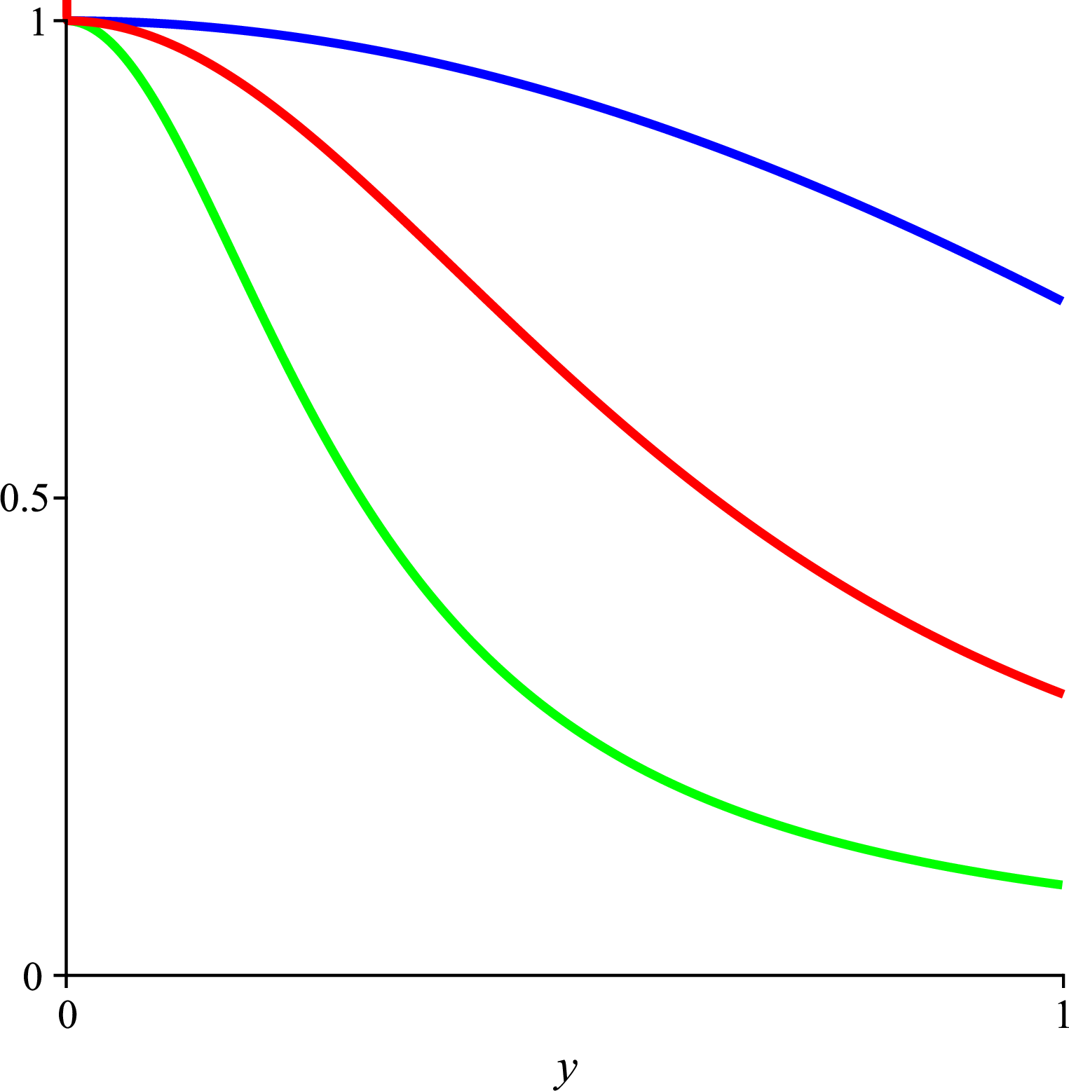
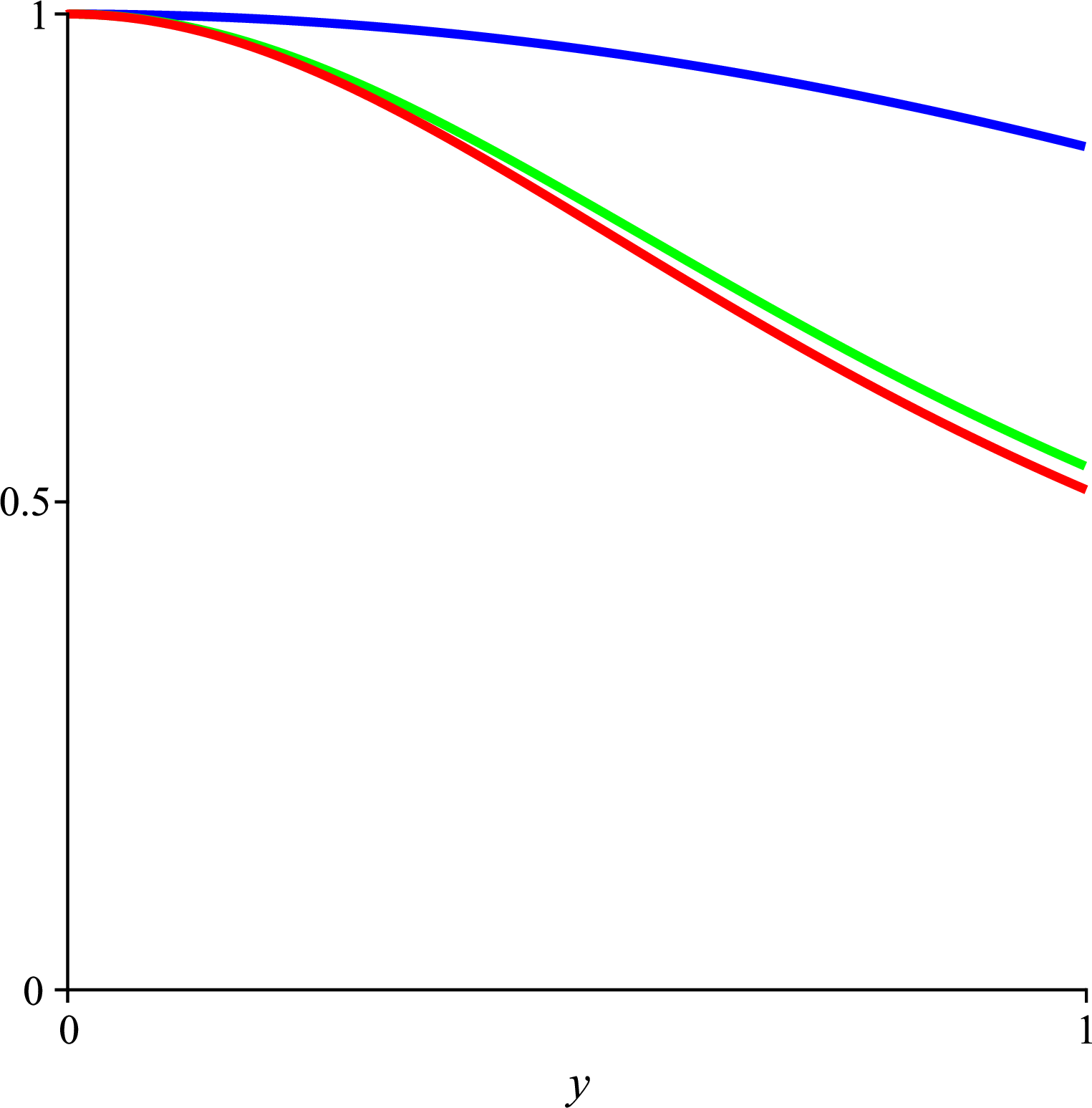
Figure 1: Profiles of \(u_{+}\) (blue), \(u_{-}\) (green), and \(u_{\ast}\) (red) in \(d=11\) (left) and \(d=21\) (right)..
4 Behavior outside the past light cone↩︎
Let \(x=1/y\). This coordinate covers the whole spacetime: the past and future light cones of the point \((t=T,r=0)\) are located at \(x=1\) and \(x=-1\) respectively, while the origin corresponds to \(x=\infty\) if \(t<T\) and \(x=-\infty\) if \(t>T\). In terms of \(x\) Eq. 7 takes the form \[\label{eqx} (1-x^2) u''(x) +(d-5) x u' -(d-2) u (1-u^2)=0.\tag{25}\] We showed above that this equation has three regular solutions in the interval \(1\leq x<\infty\), corresponding to the interior of the past light cone. The two explicit solutions \(u_{\pm}(x)\) obviously extend smoothly to the entire spacetime. That the third solution \(u_{\ast}(x)\) can be extended to \(x\in (-1,1)\) can be easily shown using the functional \[\label{Q} \tilde{H}(x)=-H(1/x)=\frac{1}{2} (1-x^2) u'(x)^2 + \frac{d-2}{4} (1-u(x)^2)^2,\tag{26}\] which satisfies \(\tilde{H}'(x)=-(d-4) x u'^2\). For \(x\rightarrow-1^{+}\), in analogy to 17 , we have \[\label{fuchs2} u_{\ast}(x)=\tilde{c}+\sum_{n=1}^{m} \tilde{c}_n (x+1)^n + \tilde{b} (x+1)^{m+1} \log(x+1) + \tilde{c}_{m+1} (x+1)^{m+1}+ \dots,\tag{27}\] with a generically nonzero coefficient \(\tilde{b}\), hence \(u_{\ast}(x)\) is only \(\mathcal{C}^{m}\) at \(x=-1\).
5 Outlook↩︎
Each smooth self-similar solution of Eq. 3 provides an example of finite-time singularity formation (“blowup") from smooth initial data. The extent to which a given self-similar solution participates in dynamics depends on its stability.
As discussed in the introduction, the solution \(u_{+}\) has been proven to be stable and has been shown numerically to govern generic blowup. The stability properties of the solutions \(u_{-}\) and \(u_{\ast}\) have not yet been established. Our ongoing work indicates that the solution \(u_{-}\) has two unstable modes for \(11 \le d \le 17\) and one for \(d \ge 19\), whereas the solution \(u_{\ast}\) exhibits the opposite behaviour, with one unstable mode for \(11 \le d \le 17\) and two for \(d \ge 19\). The solution with a single unstable mode (either \(u_{\ast}\) or \(u_{-}\), depending on the dimension) is expected to be critical, in the sense that its codimension-one stable manifold separates blowup from dispersion. This is particularly interesting in the case of solution \(u_{-}\), since its explicit form opens the door to a rigorous analysis of the threshold dynamics. Finally, we point out that for \(d\geq 10\) one can construct non-self-similar blowup solutions, in analogy with the construction of such solutions for equivariant wave maps in \(d\geq 7\) [20]. For \(d\geq 11\) these so-called type II blowup solutions have the form \(Q\left(r/\lambda(t)\right)\), where \(Q(r)\) is a static solution of Eq. 3 and \(\lambda(t)\sim (T-t)^{1+\gamma}\). The anomalous exponent \(\gamma>0\) can be determined by the method of matched asymptotics. The coexistence of type I and type II blowup scenarios for \(d\geq 10\) may lead to new blowup dynamics that are absent in lower dimensions.
Acknowledgement.↩︎
The research of P.B. was supported in part by the Polish National Science Center grant no. 2017/26/A/ST2/00530. The research of I.G. was funded in whole or in part by the Austrian Science Fund (FWF) 10.55776/PAT5825523.
Appendix↩︎
To simplify the notation, we introduce the variable \(z=c^2\). In order to count the number of zeros of the polynomials \(P_m(z)\) for \(m\geq 3\), let us first factor out the two explicit zeros corresponding to the solutions \(u_{\pm}\), \[\label{zpm} z_{\pm}=\left(1-\frac{\alpha_{\pm}}{\beta_{\pm}+1}\right)^2.\tag{28}\] Accordingly, we write \[P_m(z)=(z-z_{-})(z-z_{+}) S_m(z),\] where \[\label{Sm} S_m(z)=s_{m-2} z^{m-2}+s_{m-3} z^{m-3}+\cdots +s_0.\tag{29}\] For any finite \(m\), the coefficients \(s_0,\dots, s_{m-2}\) can be computed explicitly in an algorithmic manner. By convention, we assume that the leading coefficient \(s_{m-2}\) is positive.
The key observation (verified for increasingly large \(m\)) is that the coefficient \(s_{m-2}\) is sufficiently large, while all other coefficients \(s_{m-3},\dots,s_0\) are negative, so that \(S_m(0)<0\) and \(S_m(1)>0\). Since the sequence of coefficients \((s_{m-2},s_{m-3},\dots,s_0)\) has exactly one sign change, Descartes’ rule of signs implies that \(S_m(z)\) has exactly one positive real zero, which must lie in \((0,1)\); denote it by \(z_\ast\).
We find that \(z_{-}<z_{\ast}<z_{+}\) for \(3\leq m\leq 6\), while \(z_{\ast}<z_{-}<z_{+}\) for \(m\geq 7\). Notably, this ordering agrees with the ordering of the corresponding numbers of unstable modes mentioned in the previous section.