Differentiable Knapsack and Top-k Operators via Dynamic Programming
January 29, 2026
Abstract
Knapsack and Top-\(k\) operators are useful for selecting discrete subsets of variables. However, their integration into neural networks is challenging as they are piecewise constant, yielding gradients that are zero almost everywhere. In this paper, we propose a unified framework casting these operators as dynamic programs, and derive differentiable relaxations by smoothing the underlying recursions. On the algorithmic side, we develop efficient parallel algorithms supporting both deterministic and stochastic forward passes, and vector-Jacobian products for the backward pass. On the theoretical side, we prove that Shannon entropy is the unique regularization choice yielding permutation-equivariant operators, and characterize regularizers inducing sparse selections. Finally, on the experimental side, we demonstrate our framework on a decision-focused learning benchmark, a constrained dynamic assortment RL problem, and an extension of discrete VAEs.
1 Introduction↩︎
Many learning tasks rely on selecting a discrete subset of variables, or items, whether to learn sparse latent representations or to optimize resource allocation. The standard Top-\(k\) operator selects subsets under a fixed cardinality constraint, and the Knapsack problem [1] generalizes this structure by supporting non-uniform item weights, enforcing a total capacity limit on their sum.
While the structure of these constraints can provide necessary inductive bias, the resulting operators are piecewise constant, with either zero or undefined Jacobian. As a result, integrating them into neural networks is challenging as they break the
differentiable computation graph, preventing the backpropagation of meaningful gradients.
To bridge this gap, current research often relies on continuous relaxations or regularization for gradient estimation. Solver-agnostic, black-box approaches, such as perturbation with stochastic noise [2], [3] or piecewise affine interpolation [4], are flexible but computationally expensive, often requiring multiple solver calls. Conversely, specialized differentiable layers for ranking and Top-\(k\) operations, often based on optimal transport or regularized linear programming [5], [6], lack the generality to handle the non-uniform weights inherent to Knapsack constraints. Furthermore, many existing methods restrict the choice of regularization (e.g., to Shannon entropy), limiting control over key properties like sparsity.
In this work, we address these limitations by revisiting the structural similarities between Knapsack and Top-\(k\) problems. We cast both as instances of dynamic programming (DP), and build upon the framework of [7] to propose a unified differentiable formulation. Specifically, we make the following contributions:
In 4, we derive differentiable relaxations of the Knapsack and Top-\(k\) problems by regularizing the \(\max\) operators within the underlying Bellman DP recursions.
In 4.2, we show that Shannon entropy is the unique separable regularization function yielding permutation-equivariant relaxed operators, and characterize regularizers inducing sparse item selections ([prop:equivariance] [prop:sparsity]).
In 5.1, we derive efficient vector-Jacobian product computations, allowing the integration of the proposed operators into differentiable programming pipelines.
In 5.2, we prove the existence of a distribution underlying the proposed operators ([prop:distribution]), and provide an ancestral sampling algorithm for stochastic forward passes.
We provide a principled supervised learning approach using our operators as output layers in 5.3, by showing how to compute gradients of associated Fenchel-Young losses [8].
In 6, we compare our DP-based losses against decision-focused learning baselines, evaluate our Knapsack operators on a constrained dynamic assortment RL problem, and benchmark our proposed differentiable Top-\(k\) operators on a Fenchel-Young extension of discrete VAEs.

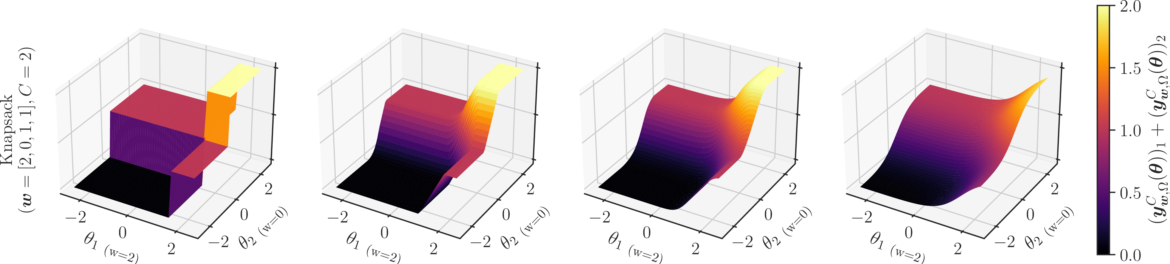
Figure 1: Illustration of our relaxed Top-\(k\) and Knapsack operators. We plot the sum of the first two coordinates of the relaxed operator for \({\boldsymbol{\theta}}=(\theta_1,\theta_2,\frac{1}{2},1)^\top\). In the first row, we use \(\boldsymbol{y}^k_{\boldsymbol{1},\Omega}\) with \(k=2\) and \({\boldsymbol{w}}=\boldsymbol{1}\). In the second row, we use \(\boldsymbol{y}^C_{\boldsymbol{w},\Omega}\) with \(C=2\) and \({\boldsymbol{w}}=(2,0,1,1)^\top\), breaking the symmetry in \(\theta_1\) and \(\theta_2\). Using \(\Omega\equiv0\) yields piecewise-constant item selections. Gini and \(1.5\)-Tsallis regularization yield a sparse a differentiable (a.e. for Gini) operator, while Shannon regularization yields a dense and differentiable one..
1.0.0.1 Notation.
We denote \([n] \triangleq \{1, \dots, n\}\). Vectors and matrices use boldface letters (e.g., \({\boldsymbol{v}}, \boldsymbol{1}, \boldsymbol{0},{\boldsymbol{M}}\)). The probability simplex in \({\mathbb{R}}^d\) is \(\triangle^d\triangleq\!\{{\boldsymbol{q}}\in{\mathbb{R}}^d_{\geq0}\mid\sum_{i}q_i\!=\!1\}\). We use \(\langle \cdot, \!\cdot \rangle\) and \(\circ\) for inner and element-wise products. The convex hull and relative interior of a set \({\mathcal{S}}\) are \({\mathsf{conv}}({\mathcal{S}})\) and \(\mathsf{ri}({\mathcal{S}})\). For a function \(f\), \(\mathsf{range}(f)\) and \(\nabla f\) are its range and gradient.
2 Background and related work↩︎
2.0.0.1 Knapsack operators.
The 0/1 Knapsack problem for \(n\) items with values given by \({\boldsymbol{\theta}}\in{\mathbb{R}}^n\), weights \({\boldsymbol{w}}\in{\mathbb{N}}^n\), and capacity \(C\in{\mathbb{N}}\), corresponds to the problem of finding a subset of items with maximal value with a total weight restricted by the maximal capacity \(C\) [1], [9]. It can be written as the following integer linear program: \[\label{pb:knapsack} \max_{{\boldsymbol{y}}\in\{0,1\}^n} \sum_{i=1}^n \theta_i y_i\quad \text{s.t.} \;\sum_{i=1}^n w_i y_i\leq C\,.\tag{1}\] We denote by \({\mathcal{Y}^C_{\boldsymbol{w}}}\triangleq\left\{ {\boldsymbol{y}}\in\{0,1\}^n\mid \langle{\boldsymbol{w}},{\boldsymbol{y}}\rangle\leq C \right\}\) the set of feasible item selections. The optimal value of Problem (1 ) is denoted by \({\mathsf{max}^C_{\boldsymbol{w}}}({\boldsymbol{\theta}})\), and \({\boldsymbol{y}^C_{\boldsymbol{w}}}({\boldsymbol{\theta}})\) is the corresponding maximizer, or Knapsack operator: \[\begin{align} {\mathsf{max}^C_{\boldsymbol{w}}}({\boldsymbol{\theta}})\triangleq \max_{{\boldsymbol{y}}\in{\mathcal{Y}^C_{\boldsymbol{w}}}}\langle{\boldsymbol{\theta}},{\boldsymbol{y}}\rangle,\quad {\boldsymbol{y}^C_{\boldsymbol{w}}}({\boldsymbol{\theta}})\triangleq\mathop{\mathrm{\mathsf{argmax}}}_{{\boldsymbol{y}}\in{\mathcal{Y}^C_{\boldsymbol{w}}}}\langle{\boldsymbol{\theta}},{\boldsymbol{y}}\rangle. \end{align}\] Danskin’s theorem gives \(\nabla{\mathsf{max}^C_{\boldsymbol{w}}}({\boldsymbol{\theta}})={\boldsymbol{y}^C_{\boldsymbol{w}}}({\boldsymbol{\theta}})\) when the maximizer is unique [10]. However, since \({\boldsymbol{y}^C_{\boldsymbol{w}}}\) is piecewise constant, its Jacobian \(\nabla_{\boldsymbol{\theta}}\boldsymbol{y}^C_{\boldsymbol{w},\Omega}({\boldsymbol{\theta}})\) is either zero or undefined, preventing the backpropagation of gradients.
2.0.0.2 Top-\(k\) operators.
The variational form of the Top-\(k\) selection problem is a notable slight variation of Problem (1 ), where item weights are given by \({\boldsymbol{w}}=\boldsymbol{1}\), and the capacity is \(C=k\) for some \(k\in[n]\). Moreover, the inequality constraint becomes an equality, so that the problem writes: \[\label{pb:topk} \max_{{\boldsymbol{y}}\in\{0,1\}^n} \sum_{i=1}^n \theta_i y_i \quad \text{s.t.}\; \sum_{i=1}^n y_i=k\,.\tag{2}\] With a slight abuse of notation (overloading Knapsack notations for \({\boldsymbol{w}}=\boldsymbol{1}\) and \(C=k\)), we respectively denote by \({\mathcal{Y}^k_{\boldsymbol{1}}}\,\), \({\mathsf{max}^k_{\boldsymbol{1}}}\,\), and \({\boldsymbol{y}^k_{\boldsymbol{1}}}\) the feasible set, value and operator in this case. Note that \({\boldsymbol{y}^k_{\boldsymbol{1}}}({\boldsymbol{\theta}})=(\mathbb{1}_{\{i\in\text{Top-k}({\boldsymbol{\theta}})\}})_{i=1}^n\) is also known as the Top-\(k\) mask of \({\boldsymbol{\theta}}\).
2.0.0.3 Smoothed maximum operators.
Let \(\Omega:\triangle^d\to{\mathbb{R}}\) be a strictly convex regularization function. The smoothed maximum operator \(\mathsf{max}_\Omega:{\mathbb{R}}^d\to{\mathbb{R}}\) is defined as: \[\mathsf{max}_\Omega({\boldsymbol{\theta}})\triangleq \max_{{\boldsymbol{q}}\in\triangle^d}\left\{ \langle{\boldsymbol{\theta}},{\boldsymbol{q}}\rangle-\Omega({\boldsymbol{q}}) \right\} = \Omega^*({\boldsymbol{\theta}}).\] Since \(\Omega\) is strictly convex, \(\mathsf{max}_\Omega\) is differentiable, with: \[\begin{align} \nabla\mathsf{max}_\Omega({\boldsymbol{\theta}})= \mathop{\mathrm{\mathsf{argmax}}}_{{\boldsymbol{q}}\in\triangle^d}\left\{ \langle{\boldsymbol{\theta}},{\boldsymbol{q}}\rangle-\Omega({\boldsymbol{q}}) \right\} = \nabla\Omega^*({\boldsymbol{\theta}}). \end{align}\] Typical choices for the regularization function \(\Omega\) include Shannon’s negative entropy, which yields the log-sum-exp operator and softmax gradients, and quadratic (or Gini’s negative entropy) regularization, which leads to the sparsemax operator [11]. This choice controls the smoothness and sparsity of the resulting operator: we discuss its consequences in our setting in 4.2.
2.0.0.4 Differentiating through combinatorial solvers.
Integrating discrete combinatorial solvers into differentiable pipelines faces the challenge of uninformative gradients, as their output is piecewise constant. A line of research differentiates the Karush-Kuhn-Tucker conditions of linear or mixed integer programs [12], [13]. One can also treat the solver as a black-box oracle. [4] propose a method to compute gradients via piecewise affine interpolation of the solver’s output. Alternatively, perturbation-based methods [2], [3] smooth the operator by adding stochastic noise to input parameters and estimate gradients via Monte-Carlo. [14] apply these perturbation techniques specifically to Top-\(k\) selection. While these approaches are flexible, they can be computationally expensive due to the need for multiple solver calls.
2.0.0.5 Differentiable Top-\(k\) and sorting.
Existing approaches typically relax Problem (2 ) using regularized optimal transport [5], [15], regularized linear programming [6], [16]–[18], or smoothed sorting networks [19], [20]. These methods, however, are deterministic and cannot be used as a stochastic layer. Closest to our work, [21] derive a differentiable Top-\(k\) operator based on factorizing the entropy of distributions on \(k\)-subsets. By adopting a broader DP-based perspective, we strictly generalize that framework: we recover similar algorithms with Shannon entropy-based regularization, and obtain new sparse operators with Gini or Tsallis regularization. Crucially, unlike all aforementioned approaches, our framework naturally handles Knapsack constraints and non-uniform weights. Furthermore, it supports both deterministic and stochastic layers.
2.0.0.6 DP for structured prediction.
In NLP, dynamic programming with the standard \((\max, +)\) semiring has been used for \(k\)-subset selection [22], [23]. Dynamic programs can be smoothed out using second-order expectation semirings [24] or by replacing \(\max\) operators in the Bellman recursion with smoothed \(\mathsf{max}_\Omega\) operators [7].
3 Knapsack and Top-\(k\) as dynamic programs↩︎
3.0.0.1 Knapsack case.
Problem (1 ) famously exhibits optimal substructure, allowing for a DP solution [1], [9]. Indeed, let \(V^{\boldsymbol{w}}[i, c]\) be the optimal value of the subproblem considering only the first \(i\leq n\) items with a capacity \(c\leq C\): \[\begin{align} V^{\boldsymbol{w}}[i,c] \triangleq \max_{{\boldsymbol{y}}\in\{0,1\}^i} \;\sum_{l=1}^i \theta_l y_l\quad \text{s.t.} \;\sum_{l=1}^i w_l y_l\leq c\,. \end{align}\] To compute this, we can compare two possible decisions for item \(i\). We can skip it and set \(y_i=0\), yielding value \(V^{\boldsymbol{w}}[i-1, c]\). Alternatively, we can pick it (only if \(w_i \leq c\)) and set \(y_i=1\), yielding value \(\theta_i+V^{\boldsymbol{w}}[i-1, c-w_i]\). This logic leads to the following recursion: \[\begin{align} \label{eq:recursion95knapsack} \!\!V^{\boldsymbol{w}}[i, c] = \begin{cases} V^{\boldsymbol{w}}[i-1, c] \quad\quad\quad\quad\quad\text{if w_{i}>c,}\\[5pt] \max\bigl( V^{\boldsymbol{w}}[i\!-\!1, c],\theta_{i}\!+\!V^{\boldsymbol{w}}[i\!-\!1,\! c\!-\!w_{i}] \bigr)\!\!\!\!\!\!\! \\ \text{else.} \end{cases} \end{align}\tag{3}\] The optimal value of Problem (1 ) is therefore given by \(V^{\boldsymbol{w}}[n, C]={\mathsf{max}^C_{\boldsymbol{w}}}({\boldsymbol{\theta}})\). This recursion runs in \(\mathcal{O}(nC)\) time and space, and is initialized with \(V^{\boldsymbol{w}}[0,\colon] = V^{\boldsymbol{w}}[\colon,0]= 0\). An illustration of this on an example is given in 10.
3.0.0.2 Top-\(k\) case.
For Problem (2 ), let \(V^{\boldsymbol{1}}[i,j]\) be the optimal value when selecting exactly \(j\) items from the first \(i\): \[\begin{align} V^{\boldsymbol{1}}[i,j] \triangleq \max_{{\boldsymbol{y}}\in\{0,1\}^i} \;\sum_{l=1}^i \theta_l y_l\quad \text{s.t.} \;\sum_{l=1}^i y_l = j\,. \end{align}\] The equality constraint implies that any subproblem \((i,j)\) with \(j>i\) is infeasible. Consequently, if item \(i\) is required to reach the target count (i.e., \(i=j\)), we are forced to pick it, as skipping would lead to an infeasible state. We enforce this behavior by initializing the boundary \(V^{\boldsymbol{1}}[0, 1\colon]\) with \(-\infty\) values, which naturally propagate to infeasible states. The \(\max\) operator then automatically discards invalid transitions, and the recursion simply writes: \[V^{\boldsymbol{1}}[i,j] = \max\left(\theta_i+ V^{\boldsymbol{1}}[i\!-\!1, j\!-\!1],\;V^{\boldsymbol{1}}[i\!-\!1, j]\right).\] The optimal value of Problem (2 ) is therefore given by \(V^{\boldsymbol{1}}[n, k] = {\mathsf{max}^k_{\boldsymbol{1}}}({\boldsymbol{\theta}})\). This recursion runs in \(\mathcal{O}(nk)\) time and space, and we illustrate it on an example in 11.
3.0.0.3 Unified framework.
Since in the Top-\(k\) setting we always have \(w_i=1\leq c\), 3 effectively serves as a unified recursion for Problems (1 ) and (2 ). The Top-\(k\) case is then simply a specific instance of the Knapsack with \({\boldsymbol{w}}=\boldsymbol{1}\) and \(C=k\), the only distinction being that the row \([0,1\colon]\) of the DP table is initialized with \(-\infty\) rather than \(0\) to enforce the strict equality constraint.
3.0.0.4 Backtracking.
These recursions yield the optimal values of Problems (1 ) and (2 ). To recover the maximizing mask \({\boldsymbol{y}^C_{\boldsymbol{w}}}({\boldsymbol{\theta}})\), one can backtrack from state \((n,C)\), i.e., iterate from \(n\) down to \(1\), and set \(y_i\) to \(0\) or \(1\) based on whether \(V^{\boldsymbol{w}}[i,c]\) was derived from a "pick" or "skip" transition.
As \({\boldsymbol{y}^C_{\boldsymbol{w}}}({\boldsymbol{\theta}})\) corresponds to a subgradient of \({\mathsf{max}^C_{\boldsymbol{w}}}({\boldsymbol{\theta}})\), this backtracking procedure is formally equivalent to a special case of backpropagation [25]. We provide a full derivation with such a differentiation viewpoint in 8.1.
4 Differentiable operators↩︎
4.1 Algorithmic smoothing↩︎
We now algorithmically smooth the dynamic programs defined in 3, by regularizing the \(\max\) operator in 3 into \(\mathsf{max}_\Omega\) using a strictly convex function \(\Omega:\triangle^2\to{\mathbb{R}}\):\[\begin{align} \label{eq:smoothed95recursion} &V^{\boldsymbol{w}}_{\Omega}[i,c] \triangleq \begin{cases} V^{\boldsymbol{w}}_{\Omega}[i-1, c] \quad \text{if w_{i}>c,}\\[0pt] \mathsf{max}_\Omega\bigl(\theta_{i}+V^{\boldsymbol{w}}_{\Omega}[i-1, c-w_{i}],\\ \quad\quad\;\;\;V^{\boldsymbol{w}}_{\Omega}[i-1, c]\bigr) \quad \text{else.} \end{cases} \end{align}\tag{4}\] In 10.3, we relate this approach to the differentiable DP framework of [7]. We now define our proposed differentiable Knapsack and Top-\(k\) operators using the smoothed recursion in 4 .
Definition 1 (Smoothed DP values and operators.). Let \({\boldsymbol{\theta}}\in{\mathbb{R}}^n\). We define the following relaxations of the Knapsack and Top-\(k\) problem values: \[\begin{align} \mathsf{max}^C_{\boldsymbol{w},\Omega}({\boldsymbol{\theta}})\triangleq V^{\boldsymbol{w}}_{\Omega}[n,C],\quad \mathsf{max}^k_{\boldsymbol{1},\Omega}({\boldsymbol{\theta}})\triangleq V^{\boldsymbol{1}}_{\Omega}[n,k], \end{align}\] as well as the corresponding smoothed operators: \[\begin{align} \boldsymbol{y}^C_{\boldsymbol{w},\Omega}({\boldsymbol{\theta}})&\triangleq \nabla\mathsf{max}^C_{\boldsymbol{w},\Omega}({\boldsymbol{\theta}})\in{\mathsf{conv}}({\mathcal{Y}^C_{\boldsymbol{w}}}),\\ \boldsymbol{y}^k_{\boldsymbol{1},\Omega}({\boldsymbol{\theta}})&\triangleq \nabla\mathsf{max}^k_{\boldsymbol{1},\Omega}({\boldsymbol{\theta}})\in{\mathsf{conv}}({\mathcal{Y}^k_{\boldsymbol{1}}}). \end{align}\]
Importantly, the smoothed values are convex in \({\boldsymbol{\theta}}\), allowing us to define convex supervised learning losses in 5.3. We prove this and other properties in 13.1.
4.1.0.1 Parallel implementation.
Observing that values \(V^{\boldsymbol{w}}_{\Omega}[i, \cdot]\) depend only on row \(i\!-\!1\), we exploit wavefront parallelism [26] by vectorizing over capacities. This reduces the effective complexity from \({\mathcal{O}}(nC)\) to \({\mathcal{O}}(n)\) parallel steps. We provide pseudo-code in 2 3, with detailed derivations given in 8.2. To achieve
high-performance execution without custom CUDA kernels, we provide a just-in-time compiled implementation in Numba [27],
efficiently parallelized over batch and capacity dimensions.

4.2 Regularization choice↩︎
We now show how regularization impacts the equivariance and sparsity of our relaxed operators. We discuss three possible choices for \(\Omega\): the Shannon, Gini, and \(1.5\)-Tsallis negative entropies [28], scaled by \(\gamma>0\): \[\begin{align} \Omega({\boldsymbol{q}})= -\gamma H^s({\boldsymbol{q}}) &\triangleq \gamma \left(q_1\log q_1 + q_2\log q_2\right),\\ \Omega({\boldsymbol{q}})= -\gamma H^g({\boldsymbol{q}})&\triangleq \frac{\gamma}{2}\left(q_1^2+q_2^2 -1\right),\\ \Omega({\boldsymbol{q}})= -\gamma H^T_{1.5}({\boldsymbol{q}})&\triangleq \frac{4\gamma}{3}\left(q_1^{\frac{3}{2}} + q_2^{\frac{3}{2}} -1\right). \end{align}\]
Shannon’s negative entropy \(\Omega=-\gamma H^s\) yields closed forms for \(\mathsf{max}^C_{\boldsymbol{w},\Omega}\) and \(\boldsymbol{y}^C_{\boldsymbol{w},\Omega}\), given in 7.1 for completeness. In 14, we derive explicit formulas for the quantities needed to instantiate 2 with these three regularization choices (\(\mathsf{max}_\Omega\) operators and their partial derivatives), which we summarize in ¿tbl:tab:instantiations?.

We now show that \(\Omega=-\gamma H^s\) ensures the permutation-equivariance of the smoothed Knapsack and Top-\(k\) operators \(\boldsymbol{y}^C_{\boldsymbol{w},\Omega}\) and \(\boldsymbol{y}^k_{\boldsymbol{1},\Omega}\). Moreover, we prove that this is in fact the only such regularization choice.
Let \(\Omega:\triangle^2\to{\mathbb{R}}\) be a convex, separable regularization function such that \(\Omega({\boldsymbol{q}})=0\) if \({\boldsymbol{q}}\in\{{\boldsymbol{e}}_1,{\boldsymbol{e}}_2\}\), and let \(S_n\) be the group of permutations. We have: \[\begin{align} &\forall (\sigma,{\boldsymbol{w}}) \in S_n\times{\mathbb{N}}^n,\;\sigma \circ \boldsymbol{y}^C_{\boldsymbol{w},\Omega}= {\boldsymbol{y}}^C_{\sigma({\boldsymbol{w}}),\Omega}\circ\sigma \\ &\boldsymbol{if and only if} \quad \Omega=-\gamma H^s \quad \text{for some}\; \gamma\geq 0. \end{align}\] In the Top-\(k\) case, since \({\boldsymbol{w}}=\boldsymbol{1}\), only item values are really permuted, giving a more compact formulation: \[\begin{align} \forall\sigma\in S_n,\;\sigma\circ\boldsymbol{y}^k_{\boldsymbol{1},\Omega}=\boldsymbol{y}^k_{\boldsymbol{1},\Omega}\circ\sigma\iff \Omega=-\gamma H^s. \end{align}\]
The proof, given in 7.2, uses the equivalence between the permutation-invariance of a function and the permutation-equivariance of its gradient, and the fact that only \(\Omega=-\gamma H^s\) yields an associative operator \(\mathsf{max}_\Omega\).
We now characterize the regularizers that enable the relaxed operators \(\boldsymbol{y}^C_{\boldsymbol{w},\Omega}\) to map to vertices \({\boldsymbol{y}}\in{\mathcal{Y}^C_{\boldsymbol{w}}}\) of the moment polytope \({\mathsf{conv}}({\mathcal{Y}^C_{\boldsymbol{w}}})\), i.e., to produce sparse item selections.
Let \(\Omega({\boldsymbol{q}}) \triangleq \sum_{i=1}^2 \omega(q_i)\) be a separable, strictly convex regularization function, with \(\omega\) differentiable on \((0,1)\). The following statements are equivalent:
The derivative of \(\omega\) is bounded on \((0,1)\), i.e.: \[\begin{align} \lim_{t\to0^+}\omega'(t) > -\infty\,, \quad \text{and} \quad \lim_{t\to1^-}\omega'(t) < +\infty. \end{align}\]
\(\boldsymbol{y}^C_{\boldsymbol{w},\Omega}\) can produce sparse item selections, i.e.: \[\begin{align} {\mathcal{Y}^C_{\boldsymbol{w}}}\subseteq\mathsf{range}(\boldsymbol{y}^C_{\boldsymbol{w},\Omega}). \end{align}\]
Furthermore, if (1) and (2) hold, define the threshold \(\tau_\Omega\triangleq \omega'(1^-)-\omega'(0^+)\), and the local advantage of skipping item \(i\!\in\![n]\) at capacity \(c\in\{w_i,\dots,C\}\) as: \[\begin{align} \Delta_{i,c}\triangleq V^{\boldsymbol{w}}_{\Omega}[i-1, c] - (\theta_i + V^{\boldsymbol{w}}_{\Omega}[i-1, c-w_i]). \end{align}\] We have: \[\begin{align} \forall c \in \{w_i,\dots,C\}, \;\Delta_{i,c}\geq \tau_\Omega \implies (\boldsymbol{y}^C_{\boldsymbol{w},\Omega}({\boldsymbol{\theta}}))_i=0\,. \end{align}\]
The proof is given in 7.3. For Gini regularization \(\Omega = \!-\gamma H^g\!\), we have \(\omega'(q)=\gamma q\), and [prop:sparsity] gives: \[\begin{align} \forall c \in \{w_i,\dots,C\}, \;\Delta_{i,c}\geq\gamma \implies (\boldsymbol{y}^C_{\boldsymbol{w},\Omega}({\boldsymbol{\theta}}))_i=0. \end{align}\] For \(\Omega\!=\!-\gamma H^T_{1.5}\), we have \(\omega'(q)=2\gamma\sqrt{q}\), giving instead: \[\begin{align} \forall c \in \{w_i,\dots,C\}, \;\Delta_{i,c}\geq 2\gamma \implies (\boldsymbol{y}^C_{\boldsymbol{w},\Omega}({\boldsymbol{\theta}}))_i=0. \end{align}\] However, for \(\Omega=-\gamma H^s\), and more generally for any Legendre-type regularizer [29] , whose gradients explode at the boundary of \(\triangle^2\), the outputs of \(\boldsymbol{y}^C_{\boldsymbol{w},\Omega}\) are forced to lie in the relative interior of the polytope \(\mathsf{ri}({\mathsf{conv}}({\mathcal{Y}^C_{\boldsymbol{w}}}))\subseteq (0,1)^n\), and therefore can never be sparse.
We illustrate these different regularization types in 1. While the surfaces in the first row suggest that \(\boldsymbol{y}^k_{\boldsymbol{1},\Omega}\) is permutation-equivariant for every \(\Omega\) (as \(\theta_1=\theta_2\) appears to be a symmetry axis), this is a visual artifact. In 12, we provide a more precise evaluation demonstrating that \(\Omega=-\gamma H^s\) (with \(\gamma\geq 0\)) is, in fact, the only regularization yielding exact equivariance, confirming [prop:equivariance].
5 Layer integration↩︎
The proposed differentiable operators can be used as hidden or output layers in any end-to-end differentiable pipeline. We denote by \({\boldsymbol{\theta}}\in{\mathbb{R}}^n\) the layer’s input, which is typically obtained as \({\boldsymbol{\theta}}=f_{W_1}({\boldsymbol{x}})\) where \(f_{W_1}\) is an upstream model with learnable parameters \(W_1\). Similarly, we denote the downstream computation graph by \(f_{W_2}\).
In [sec:continuous_forward] [sec:stochastic_forward] [sec:output_layer], we describe three principled scenarios for integration of the proposed operators into a differentiable programming framework: as a deterministic hidden layer, as a stochastic hidden layer, and as an output layer.
5.1 Deterministic forward pass and VJPs↩︎
In the hidden layer case, the most direct approach is to use the relaxed operator \(\boldsymbol{y}^C_{\boldsymbol{w},\Omega}({\boldsymbol{\theta}})\) as a deterministic, continuous layer \({\boldsymbol{\theta}}\mapsto\boldsymbol{y}^C_{\boldsymbol{w},\Omega}({\boldsymbol{\theta}})\in{\mathsf{conv}}({\mathcal{Y}^C_{\boldsymbol{w}}})\) during training, directly feeding its output to the downstream function \(f_{W_2}\).
To learn the upstream parameters \(W_1\) via backpropagation, we must compute the vector-Jacobian product (VJP) of the layer. Since \(\boldsymbol{y}^C_{\boldsymbol{w},\Omega}=\nabla\mathsf{max}^C_{\boldsymbol{w},\Omega}\), the Jacobian \(\nabla\boldsymbol{y}^C_{\boldsymbol{w},\Omega}({\boldsymbol{\theta}})\) is the Hessian \(\nabla^2\mathsf{max}^C_{\boldsymbol{w},\Omega}({\boldsymbol{\theta}})\), which is symmetric. Thus, for any cotangent vector \({\boldsymbol{z}}\in{\mathbb{R}}^n\), the VJP \({\boldsymbol{z}}^\top(\nabla_{\boldsymbol{\theta}}\boldsymbol{y}^C_{\boldsymbol{w},\Omega}({\boldsymbol{\theta}}))\) is the transpose of the JVP \((\nabla_{\boldsymbol{\theta}}\boldsymbol{y}^C_{\boldsymbol{w},\Omega}({\boldsymbol{\theta}})){\boldsymbol{z}}\).
We compute it using a reverse-over-forward approach, by backpropagating through the computation of the directional derivative \(\langle \nabla_{\boldsymbol{\theta}}\mathsf{max}^C_{\boldsymbol{w},\Omega}({\boldsymbol{\theta}}),{\boldsymbol{z}}\rangle\), which we derive in 8.3. The special structure of our DAG, which has repeated edges and constant ones, leads to important changes compared to the general case of [7] (see 10.3). The pseudo-code is given in 9, with derivations in 8.4.
In 14, we derive explicit formulas for the quantities needed to instantiate 9 with Shannon, Gini, and \(1.5\)-Tsallis regularization (\(\mathsf{max}_\Omega\) operators and their partial derivatives), which we summarize in ¿tbl:tab:instantiations?.

5.2 Stochastic forward pass and surrogate gradients↩︎
The method described in 5.1 is susceptible to a train-test mismatch. Although the network is trained on continuous vectors \(\boldsymbol{y}^C_{\boldsymbol{w},\Omega}({\boldsymbol{\theta}})\in{\mathsf{conv}}({\mathcal{Y}^C_{\boldsymbol{w}}})\), inference often requires hard item selections \({\boldsymbol{y}^C_{\boldsymbol{w}}}({\boldsymbol{\theta}}) \in {\mathcal{Y}^C_{\boldsymbol{w}}}\). This is particularly true for semantically discrete tasks where passing a soft, averaged vector \(\boldsymbol{y}^C_{\boldsymbol{w},\Omega}({\boldsymbol{\theta}})\) to \(f_{W_2}\) would be nonsensical. We propose to bridge this gap via sampling.
Let \(\boldsymbol{Q}^{\boldsymbol{w}}_{\Omega}\) be the output of 2. Let \(\pi^{\boldsymbol{w},C}_{\boldsymbol{\theta},\Omega}\) be the distribution on binary vectors defined autoregressively by: \[\begin{align} \pi^{\boldsymbol{w},C}_{\boldsymbol{\theta},\Omega}(Y_i=1|Y_{i+1},\dots, Y_n)\triangleq Q^{\boldsymbol{w}}_{\Omega}\left[i,\,C_i\right] \end{align}\] for all \(i\in\{n,\dots,1\}\), where \(C_i\triangleq C-\sum_{j=i+1}^n Y_j w_j\) is the remaining capacity for items \(\{1,\dots,i\}\).
Then, the support of \(\pi^{\boldsymbol{w},C}_{\boldsymbol{\theta},\Omega}\) is a subset of \({\mathcal{Y}^C_{\boldsymbol{w}}}\,\), and its expectation matches the relaxed operator: \[\begin{align} \boldsymbol{y}^C_{\boldsymbol{w},\Omega}({\boldsymbol{\theta}}) &= {\mathbb{E}}_{\pi^{\boldsymbol{w},C}_{\boldsymbol{\theta},\Omega}}[Y]\in{\mathsf{conv}}({\mathcal{Y}^C_{\boldsymbol{w}}}). \end{align}\] Moreover, in the scaled Shannon entropy-regularized case \(\Omega=-\gamma H^s\), we recover the Gibbs distribution: \[\begin{align} \pi^{\boldsymbol{w},C}_{\boldsymbol{\theta},\Omega}({\boldsymbol{y}}) = \frac{\exp(\langle{\boldsymbol{\theta}},{\boldsymbol{y}}\rangle/\gamma)}{\sum_{{\boldsymbol{y}}'\in{\mathcal{Y}^C_{\boldsymbol{w}}}}\exp(\langle{\boldsymbol{\theta}},{\boldsymbol{y}}'\rangle/\gamma)}. \end{align}\]
[prop:distribution], proved in 7.4, shows the existence of a distribution \(\pi^{\boldsymbol{w},C}_{\boldsymbol{\theta},\Omega}\) underlying the proposed operators, and yields a tractable \({\mathcal{O}}(n)\) ancestral sampling algorithm to sample from it. We give the pseudo-code in 4.
Moreover, the structure of \(\pi^{\boldsymbol{w},C}_{\boldsymbol{\theta},\Omega}\) enables to efficiently compute the probability of any item selection \({\boldsymbol{y}}\in{\mathcal{Y}^C_{\boldsymbol{w}}}\) as: \[\begin{align} \pi^{\boldsymbol{w},C}_{\boldsymbol{\theta},\Omega}({\boldsymbol{y}}) = \prod_{i=1}^n\left( y_iQ^{\boldsymbol{w}}_{\Omega}[i,c_i] + (1-y_i)(1-Q^{\boldsymbol{w}}_{\Omega}[i,c_i]) \right), \end{align}\] where \(c_i\triangleq C - \sum_{j=i+1}^ny_j w_j\) is the remaining capacity for items \(\{1,\dots,i\}\). This is very useful as it enables assessing the probability of a given Top-\(k\) or Knapsack assignment.
To enforce hard item selections during training, we therefore propose to replace the relaxed output \(\boldsymbol{y}^C_{\boldsymbol{w},\Omega}({\boldsymbol{\theta}})\in{\mathsf{conv}}({\mathcal{Y}^C_{\boldsymbol{w}}})\) with a discrete sample \({\boldsymbol{y}}\in {\mathcal{Y}^C_{\boldsymbol{w}}}\) from \(\pi^{\boldsymbol{w},C}_{\boldsymbol{\theta},\Omega}\) in the forward pass. To bypass the non-differentiability of the sampling operation, we adopt the following surrogate gradient approach:
During the forward pass, we treat the layer as a stochastic node by sampling \({\boldsymbol{y}}\sim\pi^{\boldsymbol{w},C}_{\boldsymbol{\theta},\Omega}\) using 4. We can then compute any loss \({\mathcal{L}}({\boldsymbol{x}}, f_{W_2}({\boldsymbol{y}}))\).
During the backward pass, we treat the layer as the deterministic node \({\boldsymbol{\theta}}\mapsto\boldsymbol{y}^C_{\boldsymbol{w},\Omega}({\boldsymbol{\theta}})={\mathbb{E}}_{\pi^{\boldsymbol{w},C}_{\boldsymbol{\theta},\Omega}}[Y]\), with VJP computed by 9. Thus, we use: \[\begin{align} \nabla_{\boldsymbol{\theta}}{\mathcal{L}}({\boldsymbol{x}}, f_{W_2}({\boldsymbol{y}}))\!\triangleq\! \left(\nabla_{\boldsymbol{\theta}}\boldsymbol{y}^C_{\boldsymbol{w},\Omega}({\boldsymbol{\theta}})\right)\!\cdot\!\nabla_{\boldsymbol{y}}{\mathcal{L}}({\boldsymbol{x}}, f_{W_2}({\boldsymbol{y}})), \end{align}\] and then backpropagate \(\nabla_{\boldsymbol{\theta}}{\mathcal{L}}({\boldsymbol{x}}, f_{W_2}({\boldsymbol{y}}))\in{\mathbb{R}}^n\) as a cotangent to upstream learnable parameters \(W_1\).
A similar "stochastic forward, deterministic backward" approach is also proposed in [21], although restricted to the Top-\(k\) setting and to the use of Shannon entropy-based regularization only (thus preventing sparsity of expected item selections and distribution supports).
5.3 Output layers and Fenchel-Young losses↩︎
We now provide a principled framework for supervised learning with the proposed operators as output layers.
5.3.0.1 Moment polytope regularization.
For any \(\Omega:\triangle^2\to{\mathbb{R}}\) used to smooth the DP recursion 3 into 4 , define the regularization function \({\Omega^C_{\boldsymbol{w}}}\) as the Fenchel conjugate of \(\mathsf{max}^C_{\boldsymbol{w},\Omega}\) with domain \({\mathsf{conv}}({\mathcal{Y}^C_{\boldsymbol{w}}})\). The corresponding Fenchel-Young loss [8] is given by: \[\begin{align} L_{{\Omega^C_{\boldsymbol{w}}}}\!: {\mathbb{R}}^n\!\times\!{\mathsf{conv}}({\Omega^C_{\boldsymbol{w}}})&\longrightarrow{\mathbb{R}}\\ ({\boldsymbol{\theta}}\,;{\boldsymbol{y}})&\longmapsto \mathsf{max}^C_{\boldsymbol{w},\Omega}({\boldsymbol{\theta}})+{\Omega^C_{\boldsymbol{w}}}({\boldsymbol{y}})\!-\!\langle{\boldsymbol{\theta}},{\boldsymbol{y}}\rangle. \end{align}\] This loss has several desirable properties [8]:
It is convex in \({\boldsymbol{\theta}}\) for all \({\boldsymbol{y}}\in{\mathcal{Y}^C_{\boldsymbol{w}}}\),
It is differentiable with gradient given by \(\nabla_{\boldsymbol{\theta}}L_{{\Omega^C_{\boldsymbol{w}}}}({\boldsymbol{\theta}}\,;{\boldsymbol{y}})=\boldsymbol{y}^C_{\boldsymbol{w},\Omega}({\boldsymbol{\theta}})-{\boldsymbol{y}}\),
It is non-negative for all \(({\boldsymbol{\theta}},{\boldsymbol{y}})\in{\mathbb{R}}^n\times{\mathsf{conv}}({\mathcal{Y}^C_{\boldsymbol{w}}})\), and equals \(0\) if and only if \({\boldsymbol{\theta}}\) is such that \(\boldsymbol{y}^C_{\boldsymbol{w},\Omega}({\boldsymbol{\theta}})={\boldsymbol{y}}\).
Thus, computing gradients reduces to computing a forward pass of the relaxed layer \(\boldsymbol{y}^C_{\boldsymbol{w},\Omega}({\boldsymbol{\theta}})\) using 3, and backpropagating the difference between its output and the ground-truth item selection \({\boldsymbol{y}}\).
6 Experiments↩︎
6.1 Decision-focused learning with Knapsack layers↩︎
We evaluate our relaxed Knapsack operator \(\boldsymbol{y}^C_{\boldsymbol{w},\Omega}\) on the PyEPO decision-focused learning benchmark [30]. Given a dataset \(({\boldsymbol{x}}^{(i)},{\boldsymbol{\theta}}^{(i)},{\boldsymbol{y}}^{(i)})_{i=1}^N\), the goal is to predict item values \(\hat{{\boldsymbol{\theta}}}^{(i)}\) from features \({\boldsymbol{x}}^{(i)}\) such that the subsequent Knapsack solution \({\boldsymbol{y}^C_{\boldsymbol{w}}}(\hat{{\boldsymbol{\theta}}}^{(i)})\) matches the ground-truth item selection \({\boldsymbol{y}}^{(i)}\). We measure performance using relative
regret, defined as \(\frac{\langle {\boldsymbol{\theta}}^{(i)},{\boldsymbol{y}}^{(i)}\rangle - \langle {\boldsymbol{\theta}}^{(i)},{\boldsymbol{y}^C_{\boldsymbol{w}}}(\hat{{\boldsymbol{\theta}}}^{(i)})\rangle}{|\langle
{\boldsymbol{\theta}}^{(i)},{\boldsymbol{y}}^{(i)}\rangle|}\).
6.1.0.1 Baselines.
We compare the losses proposed in 5.3 against six established baselines: PFY [2], DBB [4], NCE [31], and NID [32], detailed in 11.
6.1.0.2 Results.
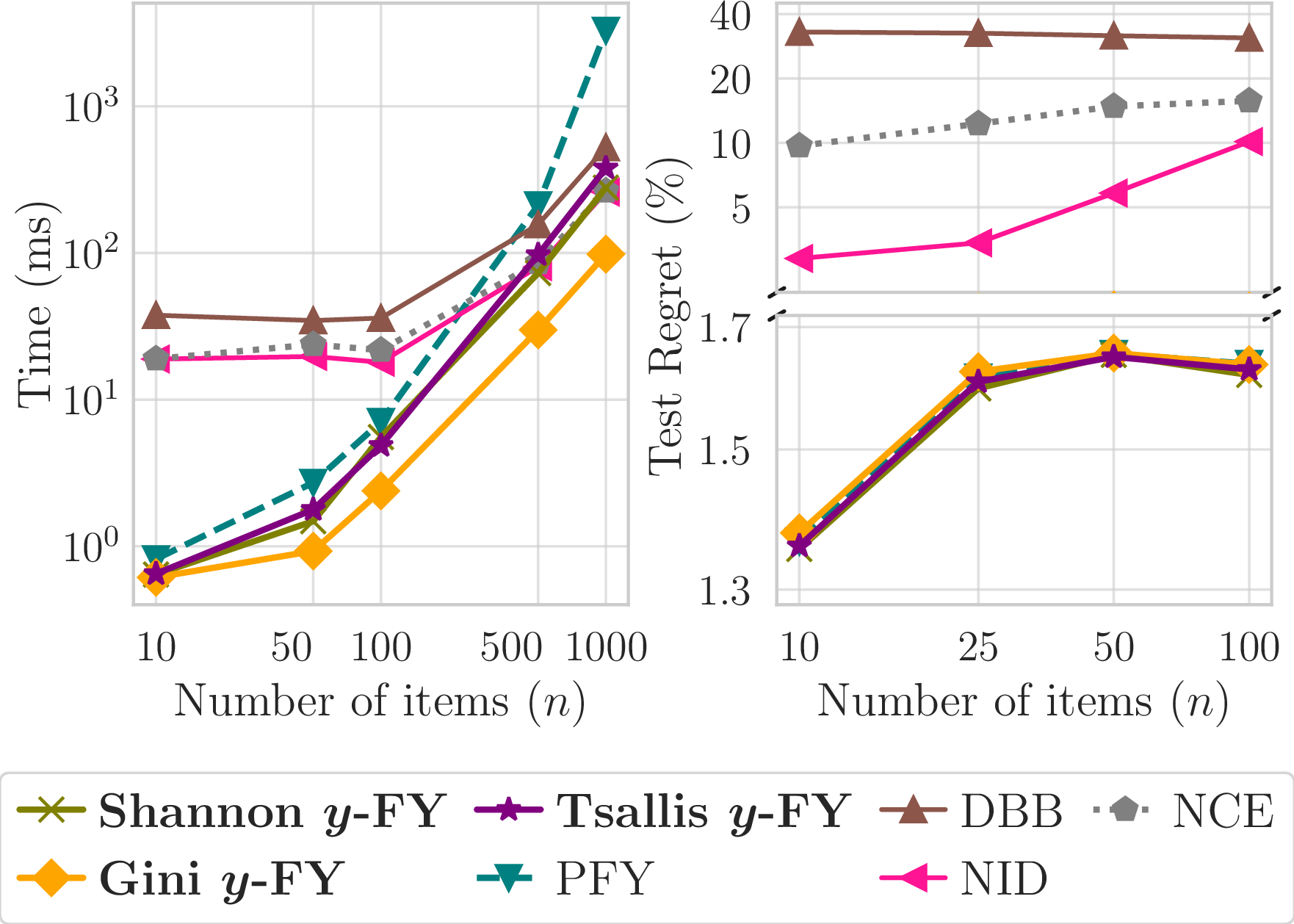
We parameterize \(\hat{{\boldsymbol{\theta}}}=f_{W_1}({\boldsymbol{x}})\) as a standard feed-forward neural network, and vary the number of items \(n\). We measure the average computation time of each evaluated loss function (forward and backward pass up to \({\boldsymbol{\theta}}\)), and the best test relative regret. The results are gathered in 5. Our DP-based Fenchel-Young losses consistently outperform the baselines in terms of regret while remaining computationally efficient. Full experimental details are given in 11.
6.2 Dynamic assortment with Knapsack constraints↩︎
We evaluate our differentiable Knapsack operators on a dynamic assortment problem [33], [34]. The agent manages a store of \(n=20\) items and selects subsets to display over \(80\) time steps, subject to capacity and inventory constraints. The environment features endogenous uncertainty driven by a hidden customer choice model, parameterized by unknown preferences \({\boldsymbol{\phi}}\). Rewards correspond to sold item prices, which deplete inventory and update features. Details are in 12.
6.2.0.1 Method.
We employ the structured RL (SRL) framework of [35], where the actor maps states to item logits \(\hat{{\boldsymbol{\theta}}}\). While the original method relies on the perturbation framework of [2] for exploration and gradient estimation, our DP-based formulation yields exact Fenchel-Young gradients \(\nabla_{\boldsymbol{\theta}}L_{{\Omega^C_{\boldsymbol{w}}}}(\hat{{\boldsymbol{\theta}}}; \hat{{\boldsymbol{y}}}) \!=\! \boldsymbol{y}^C_{\boldsymbol{w},\Omega}(\hat{{\boldsymbol{\theta}}}) \!-\! \hat{{\boldsymbol{y}}}\). Furthermore, we substitute perturbed optimization with ancestral sampling using 4 to generate targets \(\hat{{\boldsymbol{y}}}\).
6.2.0.2 Baselines.
We compare our method against standard perturbation-based SRL and PPO [36]. We also include a Greedy policy, which maximizes the cumulative price of displayed objects, and an Expert oracle. This expert "cheats" by accessing the hidden customer model \({\boldsymbol{\phi}}\) to compute the exact expected immediate revenue of every feasible assortment \({\boldsymbol{y}}\in{\mathcal{Y}^C_{\boldsymbol{w}}}\), and chooses the maximizing one. While this policy is not globally optimal (it ignores inventory and customer choice dynamics), it serves as a strong performance ceiling. Note that it is not computationally scalable, as it requires enumerating all feasible actions at every step, and \(|{\mathcal{Y}^C_{\boldsymbol{w}}}|\) grows exponentially with \(n\).
6.2.0.3 Results.
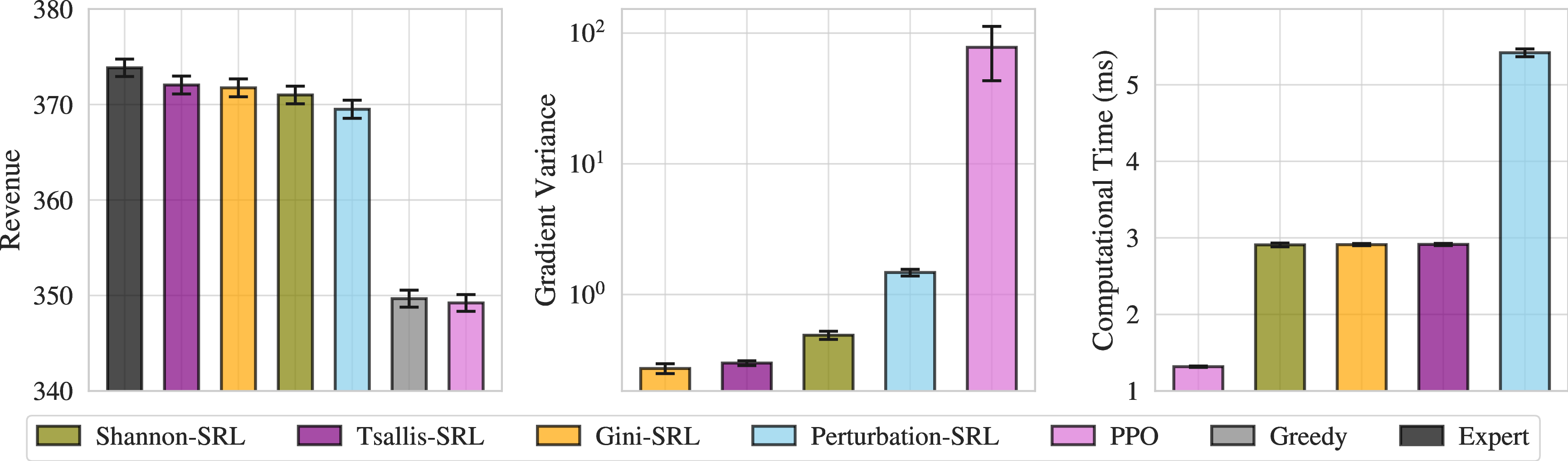
6 summarizes the results. Our DP framework significantly reduces gradient variance compared to baselines, particularly with sparse regularizers (Gini, Tsallis) which induce sparse distribution support for \(\pi^{\boldsymbol{w},C}_{\boldsymbol{\theta},\Omega}\), unlike Shannon entropy. In terms of performance, our proposed operators consistently outperform the greedy, PPO, and standard SRL baselines, with lower computational load than perturbation-based SRL for gradient estimation. Full experimental details are given in 12.
6.3 Fenchel-Young discrete VAE↩︎
We now evaluate our relaxed Top-\(k\) operators within a discrete variational auto-encoder (DVAE, [37]) framework. The goal is to learn representations that disentangle continuous style attributes from discrete categorical identity. The encoder \(E_{W_1}\) maps an input \({\boldsymbol{x}}\) to latent style parameters \({\boldsymbol{z}}_1, \dots, {\boldsymbol{z}}_n \in {\mathbb{R}}^{d_z}\) and selection logits \(\hat{{\boldsymbol{\theta}}} \in {\mathbb{R}}^n\). The discrete latent selection is obtained via either \({\boldsymbol{y}}= \boldsymbol{y}^k_{\boldsymbol{1},\Omega}(\hat{{\boldsymbol{\theta}}})\) or \({\boldsymbol{y}}\sim\pi^{\boldsymbol{1},k}_{\boldsymbol{\theta},\Omega}\) (following [sec:continuous_forward] [sec:stochastic_forward]). The reconstruction \(\hat{{\boldsymbol{x}}}\) is then generated by a shared decoder \(D_{W_2}\), which processes learnable class embeddings \({\boldsymbol{e}}_i\) conditioned on style variables \({\boldsymbol{z}}_i\), aggregated by the selection weights \({\boldsymbol{y}}\): \[\begin{align} \hat{{\boldsymbol{x}}} = \frac{1}{k} \sum_{i=1}^n y_i \cdot D_{W_2}([{\boldsymbol{e}}_i, {\boldsymbol{z}}_i]). \end{align}\] To train this model, we minimize the sum of a standard MSE reconstruction loss on \(\hat{{\boldsymbol{x}}}\), a Gaussian KL regularization term for the continuous style variables \({\boldsymbol{z}}\), and a Fenchel-Young regularization term \(L_{{\Omega^k_{\boldsymbol{1}}}}(\boldsymbol{0}\,; \boldsymbol{y}^k_{\boldsymbol{1},\Omega}(\hat{{\boldsymbol{\theta}}}))\) for the latent selection variables \({\boldsymbol{y}}\) using the DP-based loss proposed in 5.3. Full experimental details are given in 13.
As shown in 13, the Fenchel-Young regularization term \(L_{{\Omega^k_{\boldsymbol{1}}}}\) equals the standard KL divergence against an uniform prior in the \(\Omega=-H^s\) setting (thus recovering the framework of SIMPLE [21]), while enabling more general regularizers that induce sparse latent representations, such as Gini and Tsallis entropies. This formulation also extends the Fenchel-Young variational inference framework of [38], from continuous VAEs to DVAEs with latent distributions on \(k\)-subsets.
The gradient of the Fenchel-Young regularization term is given by \(\nabla_{\boldsymbol{\theta}}L_{{\Omega^k_{\boldsymbol{1}}}}(\boldsymbol{0}\,;\boldsymbol{y}^k_{\boldsymbol{1},\Omega}(\hat{{\boldsymbol{\theta}}}))=(\nabla_{\boldsymbol{\theta}}\boldsymbol{y}^k_{\boldsymbol{1},\Omega}(\hat{{\boldsymbol{\theta}}}))\cdot\hat{{\boldsymbol{\theta}}}\), i.e., it is the JVP of \(\boldsymbol{y}^k_{\boldsymbol{1},\Omega}\) in the direction of its input \(\hat{{\boldsymbol{\theta}}}\), efficiently computed via 9 (see 13 for derivations).
6.3.0.1 Experimental Setup.
We use a stacked MNIST dataset, where inputs are pixel-wise averages of \(k\!=\!3\) distinct digit images. The model must recover the identities of the constituent digits via the latent \(k\)-subset \({\boldsymbol{y}}\). We compare our deterministic and stochastic relaxed operators against the differentiable Top-\(k\) operator of [18] (FSD), as well as hard and Gumbel Top-\(k\) baselines [39], [40], trained with straight-through estimators (ST, [41]) for the backward pass.
6.3.0.2 Results.
7 illustrates the training dynamics, highlighting three results. First, our DP-based operators match or outperform baselines in reconstruction quality, with Gini and Tsallis variants significantly surpassing the Shannon-based framework of SIMPLE [21]. Second, unlike the dense Shannon-based Top-\(k\) operator, Gini and Tsallis regularization induce sparse latent representations, quickly converging to hard \(k\)-subsets to explain the data. Third, our methods exhibit superior optimization stability compared to ST-based baselines, which lead to a KL regularization term that diverges catastrophically.

Conclusion↩︎
We proposed a unified DP framework for differentiable Knapsack and Top-\(k\) operators, and proved that the regularization choice is structural for key properties such as permutation equivariance and sparsity. Our operators offer an efficient solution for enforcing combinatorial constraints in differentiable pipelines, whether as deterministic or stochastic hidden layers, or as output layers for supervised learning.
Impact statement↩︎
This paper introduces differentiable Knapsack and Top-\(k\) operators via dynamic programming. We do not foresee any specific ethical or societal implications arising directly from this work.
7 Proofs↩︎
7.1 Closed forms in the Shannon-entropy regularized case↩︎
For \(\Omega=-\gamma H^s\), we have: \[\begin{align} \mathsf{max}^C_{\boldsymbol{w},\Omega}({\boldsymbol{\theta}}) &= \gamma\cdot \log\!\!\sum_{{\boldsymbol{y}}\in{\mathcal{Y}^C_{\boldsymbol{w}}}}\exp\left(\langle {\boldsymbol{\theta}},{\boldsymbol{y}}\rangle/\gamma\right)\,,\\ \mathsf{max}^k_{\boldsymbol{1},\Omega}({\boldsymbol{\theta}}) &= \gamma\cdot \log\!\!\sum_{{\boldsymbol{y}}\in{\mathcal{Y}^k_{\boldsymbol{1}}}}\exp\left(\langle {\boldsymbol{\theta}},{\boldsymbol{y}}\rangle/\gamma\right)\,,\\ \boldsymbol{y}^C_{\boldsymbol{w},\Omega}({\boldsymbol{\theta}}) &= \sum_{{\boldsymbol{y}}\in{\mathcal{Y}^C_{\boldsymbol{w}}}}\frac{\exp\left(\langle {\boldsymbol{\theta}},{\boldsymbol{y}}\rangle/\gamma\right)}{\sum_{{\boldsymbol{y}}'\in{\mathcal{Y}^C_{\boldsymbol{w}}}}\exp\left(\langle {\boldsymbol{\theta}},{\boldsymbol{y}}'\rangle/\gamma\right)}\cdot {\boldsymbol{y}}\,,\\ \boldsymbol{y}^k_{\boldsymbol{1},\Omega}({\boldsymbol{\theta}}) &= \sum_{{\boldsymbol{y}}\in{\mathcal{Y}^k_{\boldsymbol{1}}}}\frac{\exp\left(\langle {\boldsymbol{\theta}},{\boldsymbol{y}}\rangle/\gamma\right)}{\sum_{{\boldsymbol{y}}'\in{\mathcal{Y}^k_{\boldsymbol{1}}}}\exp\left(\langle {\boldsymbol{\theta}},{\boldsymbol{y}}'\rangle/\gamma\right)}\cdot {\boldsymbol{y}}\,. \end{align}\]
Proof. For any integer \(d\geq2\), define \(\Omega_d:\triangle^{d}\to{\mathbb{R}}\) as \(\Omega_d({\boldsymbol{q}})\triangleq \gamma \sum_{i=1}^dq_i\log q_i\). [7] gives that this definition of the family \((\Omega_d)_{d\geq 2}\) is such that: \[\begin{align} \mathsf{max}^C_{{\boldsymbol{w}},\Omega_2}({\boldsymbol{\theta}}) = \mathsf{max}_{\Omega_{|{\mathcal{Y}^C_{\boldsymbol{w}}}|}}({\boldsymbol{s}}_{{\boldsymbol{\theta}}}), \end{align}\] where we define the score vector \({\boldsymbol{s}}_{{\boldsymbol{\theta}}}\triangleq \left(\langle{\boldsymbol{\theta}},{\boldsymbol{y}}\rangle\right)_{{\boldsymbol{y}}\in{\mathcal{Y}^C_{\boldsymbol{w}}}}\). To make the bridges between notations clearer, [7] use a generic, dimension-agnostic definition of the regularizer \(\Omega\), and \(\mathsf{max}^C_{{\boldsymbol{w}},\Omega_2}({\boldsymbol{\theta}})\) and \(\max_{\Omega_{|{\mathcal{Y}^C_{\boldsymbol{w}}}|}}({\boldsymbol{s}}_{{\boldsymbol{\theta}}})\) are denoted by \(\mathrm{DP}_\Omega({\boldsymbol{\theta}})\) and \(\mathrm{LP}_\Omega({\boldsymbol{\theta}})\), respectively.
Moreover, since we have the closed form \(\mathsf{max}_{\Omega_d}({\boldsymbol{q}})=\gamma \log\sum_{i=1}^d \exp(q_i/\gamma)\) for any \(d\geq2\), we get:
\[\begin{align} {\boldsymbol{y}}^C_{{\boldsymbol{w}},\Omega_2}({\boldsymbol{\theta}}) &= \nabla_{\boldsymbol{\theta}}\mathsf{max}^C_{{\boldsymbol{w}},\Omega_2}({\boldsymbol{\theta}})\\ &= \nabla_{\boldsymbol{\theta}}\mathsf{max}_{\Omega_{|{\mathcal{Y}^C_{\boldsymbol{w}}}|}}({\boldsymbol{s}}_{{\boldsymbol{\theta}}})\\ &= \nabla_{\boldsymbol{\theta}}\left( \gamma\log\!\!\!\sum_{{\boldsymbol{y}}\in{\mathcal{Y}^C_{\boldsymbol{w}}}}\!\!\exp\left( \langle{\boldsymbol{\theta}},{\boldsymbol{y}}\rangle/\gamma \right) \right)\\ &= \sum_{{\boldsymbol{y}}\in{\mathcal{Y}^C_{\boldsymbol{w}}}}\frac{\exp\left(\langle {\boldsymbol{\theta}},{\boldsymbol{y}}\rangle/\gamma\right)}{\sum_{{\boldsymbol{y}}'\in{\mathcal{Y}^C_{\boldsymbol{w}}}}\exp\left(\langle {\boldsymbol{\theta}},{\boldsymbol{y}}'\rangle/\gamma\right)}\cdot {\boldsymbol{y}}\,. \end{align}\]
While we wrote the proof only in Knapsack notation, since the differences in the padding values initializing the table \(\boldsymbol{V}^{\boldsymbol{w}}_{\Omega}\) (which is the only distinction between the Knapsack and the Top-\(k\) cases) do not impact it, the exact same arguments naturally hold for \(\boldsymbol{y}^k_{\boldsymbol{1},\Omega}\). ◻
7.2 Proof of [prop:equivariance] ()↩︎
Proof. \(\bullet\) (\(\implies\))
First, we show the equivariance of \(\boldsymbol{y}^C_{\boldsymbol{w},\Omega}\) with respect to permutations of \({\boldsymbol{\theta}}\) and \({\boldsymbol{w}}\) for \(\Omega=-\gamma H^s\). First, we assume \(\gamma >0\). In this setting, we have the following closed form: \[\begin{align} \boldsymbol{y}^C_{\boldsymbol{w},\Omega}({\boldsymbol{\theta}}) &= \sum_{{\boldsymbol{y}}\in{\mathcal{Y}^C_{\boldsymbol{w}}}}\frac{\exp\left(\langle {\boldsymbol{\theta}},{\boldsymbol{y}}\rangle/\gamma\right)}{\sum_{{\boldsymbol{y}}'\in{\mathcal{Y}^C_{\boldsymbol{w}}}}\exp\left(\langle {\boldsymbol{\theta}},{\boldsymbol{y}}'\rangle/\gamma\right)}\cdot {\boldsymbol{y}}\,. \end{align}\] Let \(\sigma\in S_n\). We then have: \[\begin{align} {\boldsymbol{y}}^C_{\sigma({\boldsymbol{w}}),\Omega}\left(\sigma({\boldsymbol{\theta}})\right) = \sum_{{\boldsymbol{y}}\in\mathcal{Y}^C_{\sigma({\boldsymbol{w}})}}\frac{\exp\left(\langle \sigma({\boldsymbol{\theta}}),{\boldsymbol{y}}\rangle/\gamma\right)}{\sum_{{\boldsymbol{y}}'\in\mathcal{Y}^C_{\sigma({\boldsymbol{w}})}}\exp\left(\langle \sigma({\boldsymbol{\theta}}),{\boldsymbol{y}}'\rangle/\gamma\right)}\cdot {\boldsymbol{y}}\,. \end{align}\] Let us recall that the action of the permutation \(\sigma\) on \({\mathbb{R}}^n\) is that of an orthogonal endomorphism, giving: \[\begin{align} \forall {\boldsymbol{u}},{\boldsymbol{v}}\in{\mathbb{R}}^n,\quad \langle\sigma({\boldsymbol{u}}),{\boldsymbol{v}}\rangle=\langle{\boldsymbol{u}},\sigma^{-1}({\boldsymbol{v}})\rangle,\quad \text{and} \quad \langle\sigma({\boldsymbol{u}}),\sigma({\boldsymbol{v}})\rangle=\langle{\boldsymbol{u}},{\boldsymbol{v}}\rangle. \end{align}\] Then, by definition of the feasible item selection set, we have: \[\begin{align} \mathcal{Y}^C_{\sigma({\boldsymbol{w}})} &= \left\{ {\boldsymbol{y}}\in\{0,1\}^n\mid \langle\sigma({\boldsymbol{w}}),{\boldsymbol{y}}\rangle\leq C \right\}\\ &= \left\{ {\boldsymbol{y}}\in\{0,1\}^n\mid \langle{\boldsymbol{w}},\sigma^{-1}({\boldsymbol{y}})\rangle\leq C \right\}\\ &= \left\{ \sigma({\boldsymbol{y}}')\mid {\boldsymbol{y}}'\in\{0,1\}^n,\; \langle{\boldsymbol{w}},{\boldsymbol{y}}'\rangle\leq C \right\} &&\text{(since \sigma^{-1}(\{0,1\}^n)=\{0,1\}^n)}\\ &= \left\{ \sigma({\boldsymbol{y}}') \mid {\boldsymbol{y}}'\in {\mathcal{Y}^C_{\boldsymbol{w}}}\right\}, \end{align}\] where we denote \(\sigma^{-1}({\boldsymbol{y}})\mathrel{\vcenter{:}}={\boldsymbol{y}}'\) for clarity.
Thus, we have in fact: \[\begin{align} {\boldsymbol{y}}^C_{\sigma({\boldsymbol{w}}),\Omega}\left(\sigma({\boldsymbol{\theta}})\right) &= \sum_{{\boldsymbol{y}}\in\mathcal{Y}^C_{\sigma({\boldsymbol{w}})}}\frac{\exp\left(\langle \sigma({\boldsymbol{\theta}}),{\boldsymbol{y}}\rangle/\gamma\right)}{\sum_{{\boldsymbol{y}}'\in\mathcal{Y}^C_{\sigma({\boldsymbol{w}})}}\exp\left(\langle \sigma({\boldsymbol{\theta}}),{\boldsymbol{y}}'\rangle/\gamma\right)}\cdot {\boldsymbol{y}}\\ &= \sum_{{\boldsymbol{y}}'\in{\mathcal{Y}^C_{\boldsymbol{w}}}}\frac{\exp\left(\langle \sigma({\boldsymbol{\theta}}),\sigma({\boldsymbol{y}}')\rangle/\gamma\right)}{\sum_{{\boldsymbol{y}}''\in{\mathcal{Y}^C_{\boldsymbol{w}}}}\exp\left(\langle \sigma({\boldsymbol{\theta}}),\sigma({\boldsymbol{y}}'')\rangle/\gamma\right)}\cdot \sigma({\boldsymbol{y}}')\\ &= \sum_{{\boldsymbol{y}}'\in{\mathcal{Y}^C_{\boldsymbol{w}}}}\frac{\exp\left(\langle {\boldsymbol{\theta}},{\boldsymbol{y}}'\rangle/\gamma\right)}{\sum_{{\boldsymbol{y}}''\in{\mathcal{Y}^C_{\boldsymbol{w}}}}\exp\left(\langle {\boldsymbol{\theta}},{\boldsymbol{y}}''\rangle/\gamma\right)}\cdot \sigma({\boldsymbol{y}}')\\ &= \sigma\left(\sum_{{\boldsymbol{y}}'\in{\mathcal{Y}^C_{\boldsymbol{w}}}}\frac{\exp\left(\langle {\boldsymbol{\theta}},{\boldsymbol{y}}'\rangle/\gamma\right)}{\sum_{{\boldsymbol{y}}''\in{\mathcal{Y}^C_{\boldsymbol{w}}}}\exp\left(\langle {\boldsymbol{\theta}},{\boldsymbol{y}}''\rangle/\gamma\right)}\cdot {\boldsymbol{y}}'\right)\\ &= \sigma\left( \boldsymbol{y}^C_{\boldsymbol{w},\Omega}({\boldsymbol{\theta}}) \right). \end{align}\] For the Top-\(k\) case, the exact same arguments hold, and the final expression of equivariance is only simplified because \(\sigma({\boldsymbol{w}})={\boldsymbol{w}}\) as \({\boldsymbol{w}}=\boldsymbol{1}\).
Second, for the case \(\gamma=0\), we recover the unregularized operators, i.e., \(\boldsymbol{y}^C_{\boldsymbol{w},\Omega}={\boldsymbol{y}^C_{\boldsymbol{w}}}\) and \(\boldsymbol{y}^k_{\boldsymbol{1},\Omega}={\boldsymbol{y}^k_{\boldsymbol{1}}}\), so that the equivariance property is simply directly implied by their definition as maximizers in Problems (1 ) and (2 ).
\(\bullet\) (\(\impliedby\))
We now show that Shannon’s negative entropy is the only choice of a convex, separable regularizer yielding permutation-equivariant relaxed operators.
Let \(\Omega:\triangle^2\to{\mathbb{R}}\) be a convex regularization function. We assume it is separable, i.e., such that \(\Omega({\boldsymbol{q}})= \omega(q_1)+\omega(q_2)\) for some lower semi-continuous convex function \(\omega:[0,1]\to{\mathbb{R}}\). Moreover, we assume that \(\Omega({\boldsymbol{q}})=0\) for \({\boldsymbol{q}}\in\{{\boldsymbol{e}}_1,{\boldsymbol{e}}_2\}\) (i.e., \(\omega(0)+\omega(1)=0\)), and that \(\Omega\) yields the permutation-equivariance property for the relaxed layers, i.e., that we have: \[\begin{align} \forall(\sigma,{\boldsymbol{\theta}},{\boldsymbol{w}})\in S_n\times {\mathbb{R}}^n\times {\mathbb{N}}^n, \quad {\boldsymbol{y}}^C_{\sigma({\boldsymbol{w}}),\Omega}(\sigma({\boldsymbol{\theta}})) &= \sigma\left({\boldsymbol{y}}^C_{{\boldsymbol{w}},\Omega}({\boldsymbol{\theta}})\right),\\ {\boldsymbol{y}}^k_{\boldsymbol{1},\Omega}(\sigma({\boldsymbol{\theta}})) &= \sigma\left({\boldsymbol{y}}^k_{\boldsymbol{1},\Omega}({\boldsymbol{\theta}})\right). \end{align}\]
We must show that we then necessarily have \(\Omega=-\gamma H^s\) for some \(\gamma\geq 0\). In fact, we will show that \(\Omega\) must necessarily yield an associative smoothed maximum operator \(\mathsf{max}_\Omega\): indeed, both are equivalent by Lemma 3 in [7].
More precisely, we will assume that \(\mathsf{max}_\Omega\) is not associative for the sake of contradiction, and show that the permutation-equivariance property cannot be verified.
To do so, 1 2 will prove useful.
Lemma 1. Let \(\Omega:\triangle^2\to{\mathbb{R}}\) be convex, with \(\Omega({\boldsymbol{q}})=\omega(q_1)+\omega(q_2)\), where \(\omega:[0,1]\to{\mathbb{R}}\) is lower semi-continuous, and such that \(\Omega({\boldsymbol{q}})=0\) for \({\boldsymbol{q}}\in\{{\boldsymbol{e}}_1,{\boldsymbol{e}}_2\}\). We have, for any \(x\in{\mathbb{R}}\): \[\begin{align} \lim_{c\to+\infty}\mathsf{max}_\Omega(x+c, 0)-c = x\,. \end{align}\]
Lemma 2. Let \(f:{\mathbb{R}}^n\to{\mathbb{R}}\) be any differentiable function. Then, we have: \[\begin{align} f\circ\sigma=f \quad \text{for all \sigma\in S_n} \quad \iff \quad \nabla f\circ \sigma =\sigma\circ\nabla f \quad \text{for all \sigma\in S_n\,.} \end{align}\] That is, a differentiable function is permutation-invariant if and only if its gradient is permutation-equivariant.
We give a proof of 1 2 in [proof:limit] [proof:equiv] for completeness. We now build simple instances of the Top-\(k\) and Knapsack problems for which we show that the associativity of \(\mathsf{max}_\Omega\) is implied by the permutation-equivariance assumption for \({\boldsymbol{y}}^C_{{\boldsymbol{w}},\Omega}\) and \({\boldsymbol{y}}^k_{\boldsymbol{1},\Omega}\).
Knapsack case. Let \(n=3\), \({\boldsymbol{w}}=\boldsymbol{1}\), \(C=1\). The smoothed dynamic program for solving the corresponding Knapsack problem with \({\boldsymbol{x}}=(x_1,x_2,x_3)\in{\mathbb{R}}^3\) is depicted in 8. Unrolling the smoothed recursion from 4 gives: \[\begin{align} \mathsf{max}^C_{\boldsymbol{w},\Omega}({\boldsymbol{x}}) &= V^{\boldsymbol{w}}_{\Omega}[3,1]\\ &= \mathsf{max}_\Omega\left( x_3 + 0, V^{\boldsymbol{w}}_{\Omega}[2,1] \right)\\ &= \mathsf{max}_\Omega\left( x_3, \mathsf{max}_\Omega\left( x_2 + 0, V^{\boldsymbol{w}}_{\Omega}[1,1] \right) \right)\\ &= \mathsf{max}_\Omega\left( x_3, \mathsf{max}_\Omega\left( x_2, \mathsf{max}_\Omega\left( x_1, 0\right) \right) \right). \end{align}\] Moreover, since \(\Omega\) is separable, it is commutative, so that \(\mathsf{max}_\Omega\) is also commutative. Thus, we get: \[\begin{align} \mathsf{max}^C_{\boldsymbol{w},\Omega}({\boldsymbol{x}}) = \mathsf{max}_\Omega\left( \mathsf{max}_\Omega\left(\mathsf{max}_\Omega\left(x_1, 0\right) , x_2\right), x_3\right). \end{align}\] Now let \(\sigma\in S_3\) be defined by \(\sigma((x_1, x_2, x_3)) = (x_3, x_2, x_1)\) for all \({\boldsymbol{x}}\in{\mathbb{R}}^3\). We have, similarly: \[\begin{align} \mathsf{max}^C_{\sigma({\boldsymbol{w}}),\Omega}(\sigma({\boldsymbol{x}}))&=\mathsf{max}^C_{\boldsymbol{w},\Omega}(\sigma({\boldsymbol{x}})) &&\text{(since {\boldsymbol{w}}=\boldsymbol{1}, so \sigma({\boldsymbol{w}})={\boldsymbol{w}})} \\ &= \mathsf{max}_\Omega\left( x_1, \mathsf{max}_\Omega\left( x_2, \mathsf{max}_\Omega\left( x_3, 0\right) \right) \right). \end{align}\] Since we assumed for the sake of contradiction that \(\mathsf{max}_\Omega\) is not associative, we can find \((\theta_1,\theta_2,\theta_3)\in{\mathbb{R}}^3\) such that \(\mathsf{max}_\Omega\left(\mathsf{max}_\Omega\left( \theta_1, \theta_2 \right),\theta_3 \right)\neq \mathsf{max}_\Omega\left(\theta_1,\mathsf{max}_\Omega\left( \theta_2, \theta_3 \right) \right)\). However, from what precedes, and using the distributivity of \(+\) over \(\mathsf{max}_\Omega\), we also get, for any \(c\in{\mathbb{R}}\): \[\begin{align} \mathsf{max}^C_{\boldsymbol{w},\Omega}({\boldsymbol{\theta}}+c\boldsymbol{1}) &= \mathsf{max}_\Omega\left( \mathsf{max}_\Omega\left(\mathsf{max}_\Omega\left(\theta_1+c, 0\right) , \theta_2+c\right), \theta_3+c\right)\\ &= c+\mathsf{max}_\Omega\left( \mathsf{max}_\Omega\left(\mathsf{max}_\Omega\left(\theta_1+c, 0\right)-c , \theta_2\right), \theta_3\right),\\ \mathsf{max}^C_{\boldsymbol{w},\Omega}(\sigma({\boldsymbol{\theta}}+c\boldsymbol{1})) &= \mathsf{max}_\Omega\left(\theta_1+c, \mathsf{max}_\Omega\left(\theta_2+c, \mathsf{max}_\Omega\left(\theta_3+c, 0\right) \right) \right)\\ &= c+\mathsf{max}_\Omega\left(\theta_1, \mathsf{max}_\Omega\left(\theta_2, \mathsf{max}_\Omega\left(\theta_3+c, 0\right)-c \right) \right). \end{align}\] Thus, we have, for any \(c\in{\mathbb{R}}\): \[\begin{align} \mathsf{max}^C_{\boldsymbol{w},\Omega}({\boldsymbol{\theta}}+c\boldsymbol{1})-c &= \mathsf{max}_\Omega\left( \mathsf{max}_\Omega\left(\mathsf{max}_\Omega\left(\theta_1+c, 0\right)-c , \theta_2\right), \theta_3\right),\\ \mathsf{max}^C_{\boldsymbol{w},\Omega}(\sigma({\boldsymbol{\theta}}+c\boldsymbol{1})) -c &= \mathsf{max}_\Omega\left(\theta_1, \mathsf{max}_\Omega\left(\theta_2, \mathsf{max}_\Omega\left(\theta_3+c, 0\right)-c \right) \right). \end{align}\] By 1, we have: \[\begin{align} \mathsf{max}_\Omega\left(\theta_1+c, 0\right)-c&\xrightarrow[c\to+\infty]{}\theta_1,\\ \mathsf{max}_\Omega\left(\theta_3+c, 0\right)-c&\xrightarrow[c\to+\infty]{}\theta_3. \end{align}\] Since \(\mathsf{max}_\Omega\) is continuous, we can take the limit of the previous expressions: \[\begin{align} \lim_{c\to+\infty}\mathsf{max}^C_{\boldsymbol{w},\Omega}({\boldsymbol{\theta}}+c\boldsymbol{1})-c &= \mathsf{max}_\Omega\left( \mathsf{max}_\Omega\left(\theta_1 , \theta_2\right), \theta_3\right),\\ \lim_{c\to+\infty}\mathsf{max}^C_{\boldsymbol{w},\Omega}(\sigma({\boldsymbol{\theta}}+c\boldsymbol{1})) -c &= \mathsf{max}_\Omega\left(\theta_1, \mathsf{max}_\Omega\left(\theta_2, \theta_3 \right) \right). \end{align}\] Thus, by our definition of \({\boldsymbol{\theta}}\), we have: \[\begin{align} \lim_{c\to+\infty}\mathsf{max}^C_{\boldsymbol{w},\Omega}({\boldsymbol{\theta}}+c\boldsymbol{1})-c \neq \lim_{c\to+\infty}\mathsf{max}^C_{\boldsymbol{w},\Omega}(\sigma({\boldsymbol{\theta}}+c\boldsymbol{1})) -c. \end{align}\]
Thus, we necessarily have: \[\begin{align} \exists c\in{\mathbb{R}}: \quad \mathsf{max}^C_{\boldsymbol{w},\Omega}({\boldsymbol{\theta}}+c\boldsymbol{1})\neq\mathsf{max}^C_{\boldsymbol{w},\Omega}(\sigma({\boldsymbol{\theta}}+c\boldsymbol{1})). \end{align}\] Further, since \(\boldsymbol{y}^C_{\boldsymbol{w},\Omega}=\nabla\mathsf{max}^C_{\boldsymbol{w},\Omega}\), 2 gives that this prevents us from having \(\sigma(\boldsymbol{y}^C_{\boldsymbol{w},\Omega}({\boldsymbol{x}}))=\boldsymbol{y}^C_{\boldsymbol{w},\Omega}(\sigma({\boldsymbol{x}}))\) for all \({\boldsymbol{x}}\in{\mathbb{R}}^n\), which contradicts the permutation-equivariance assumption (since we have \({\boldsymbol{w}}=\sigma({\boldsymbol{w}})=\boldsymbol{1}\)).
Top-\(k\) case. Let \(n=3\), \(k=1\). The smoothed dynamic program for solving the corresponding Knapsack problem with input \({\boldsymbol{x}}=({\boldsymbol{x}}_1,{\boldsymbol{x}}_2,{\boldsymbol{x}}_3)\in{\mathbb{R}}^3\) is depicted in 8. Unrolling the smoothed recursion from 4 gives: \[\begin{align} \mathsf{max}^k_{\boldsymbol{1},\Omega}({\boldsymbol{x}}) &= V^{\boldsymbol{1}}_{\Omega}[3,1]\\ &= \mathsf{max}_\Omega\left( x_3 + 0, V^{\boldsymbol{1}}_{\Omega}[2,1] \right)\\ &= \mathsf{max}_\Omega\left( x_3, \mathsf{max}_\Omega\left( x_2 + 0, V^{\boldsymbol{1}}_{\Omega}[1,1] \right) \right)\\ &= \mathsf{max}_\Omega\left( x_3, \mathsf{max}_\Omega\left( x_2, \mathsf{max}_\Omega\left( x_1, -\infty\right) \right) \right). \end{align}\] From the definition of smoothed maximum operators, we can easily see that \(\mathsf{max}_\Omega(x,-\infty)=x - \Omega({\boldsymbol{e}}_1)\) for all \(x\in{\mathbb{R}}\), since the maximizing distribution in the definition of \(\mathsf{max}_\Omega\) is necessarily \({\boldsymbol{q}}={\boldsymbol{e}}_1\). Moreover, since we assumed \(\Omega({\boldsymbol{q}})=0\) when \({\boldsymbol{q}}\in\{{\boldsymbol{e}}_1,{\boldsymbol{e}}_2\}\), we have \(\mathsf{max}_\Omega(x,-\infty)=x\). Thus, we get in fact: \[\begin{align} \mathsf{max}^k_{\boldsymbol{1},\Omega}({\boldsymbol{x}}) &= \mathsf{max}_\Omega\left( x_3, \mathsf{max}_\Omega\left( x_2, x_1\right) \right)\\ &= \mathsf{max}_\Omega\left(\mathsf{max}_\Omega\left( x_1, x_2 \right),x_3 \right), \end{align}\] where we also used commutativity of \(\mathsf{max}_\Omega\). Now let \(\sigma\in S_3\) be defined by \(\sigma((x_1, x_2, x_3)) = (x_3, x_2, x_1)\) for all \({\boldsymbol{x}}\in{\mathbb{R}}^3\). We have, similarly: \[\begin{align} \mathsf{max}^k_{\boldsymbol{1},\Omega}(\sigma({\boldsymbol{x}})) &= \mathsf{max}_\Omega\left(\mathsf{max}_\Omega\left( x_3, x_2 \right),x_1 \right)\\ &= \mathsf{max}_\Omega\left(x_1,\mathsf{max}_\Omega\left(x_2, x_3\right) \right). \end{align}\] Since we assumed for the sake of contradiction that \(\mathsf{max}_\Omega\) is not associative, we can find \((\theta_1,\theta_2,\theta_3)\in{\mathbb{R}}^3\) such that \(\mathsf{max}_\Omega\left(\mathsf{max}_\Omega\left( \theta_1, \theta_2 \right),\theta_3 \right)\neq \mathsf{max}_\Omega\left(\theta_1,\mathsf{max}_\Omega\left( \theta_2, \theta_3 \right) \right)\). Thus, from previous calculations, we then have \(\mathsf{max}^k_{\boldsymbol{1},\Omega}({\boldsymbol{\theta}})\neq \mathsf{max}^k_{\boldsymbol{1},\Omega}(\sigma({\boldsymbol{\theta}}))\). Further, from 2, since \(\boldsymbol{y}^k_{\boldsymbol{1},\Omega}=\nabla\mathsf{max}^k_{\boldsymbol{1},\Omega}\), this prevents us from having \(\boldsymbol{y}^k_{\boldsymbol{1},\Omega}(\sigma({\boldsymbol{\theta}}))=\sigma(\boldsymbol{y}^k_{\boldsymbol{1},\Omega}({\boldsymbol{\theta}}))\) for all \({\boldsymbol{\theta}}\in{\mathbb{R}}^3\), which contradicts the permutation-equivariance assumption.
◻
7.3 Proof of [prop:sparsity] ()↩︎
Proof. \(\bullet\) Equivalence. First, we prove the equivalence between the boundedness of \(\omega'\) and the surjectivity of \(\boldsymbol{y}^C_{\boldsymbol{w},\Omega}\) onto the vertices \({\mathcal{Y}^C_{\boldsymbol{w}}}\) of the moment polytope.
\(\bullet\) (1) \(\implies\) (2). Assume \(\omega'\) is bounded at the endpoints. We show that \({\mathcal{Y}^C_{\boldsymbol{w}}}\subseteq\mathsf{range}(\boldsymbol{y}^C_{\boldsymbol{w},\Omega})\).
As shown in [8], since \(\omega'\) is bounded, the local gradient mapping \(\nabla \mathsf{max}_\Omega\) has a finite saturation threshold. Specifically, let \(\tau_\Omega \triangleq \lim_{t \to 1^-} \{\omega'(t)\} - \lim_{t \to 0^+} \{\omega'(t)\} < \infty\). For any inputs \(a, b \in {\mathbb{R}}\), if the gap \(|a-b| \geq \tau_\Omega\), the regularized maximizer saturates to a hard decision: \[\begin{align} \label{eq:saturation} a - b \geq \tau_\Omega \implies (\nabla \mathsf{max}_\Omega(a,b))_1 = 1, \quad b - a \geq \tau_\Omega \implies (\nabla \mathsf{max}_\Omega(a,b))_1 = 0. \end{align}\tag{5}\]
We now establish a bound on the difference between the values of the smoothed and hard DP tables.
Lemma 3. Let \(M_\Omega \triangleq \sup_{{\boldsymbol{q}}\in \triangle^2} |\Omega({\boldsymbol{q}})| < \infty\). For any \({\boldsymbol{\theta}}\in {\mathbb{R}}^n\), \(i \in \{0, \dots, n\},\;c\in\{0,\dots,C\}\), we have: \[\begin{align} \left\lvert V^{\boldsymbol{w}}_{\Omega}[i,c]({\boldsymbol{\theta}}) - V^{\boldsymbol{w}}[i,c]({\boldsymbol{\theta}}) \right\rvert \leq i M_\Omega. \end{align}\]
We prove 3 by induction in 7.7.
Now let \({\boldsymbol{y}}\in {\mathcal{Y}^C_{\boldsymbol{w}}}\) be an arbitrary feasible item selection. As \({\boldsymbol{y}}\) is a vertex of the polytope \({\mathsf{conv}}({\mathcal{Y}^C_{\boldsymbol{w}}})\), there exists a score vector \({\boldsymbol{s}}\in {\mathbb{R}}^n\) such that: \[\begin{align} {\boldsymbol{y}}=\mathop{\mathrm{\mathsf{argmax}}}_{{\boldsymbol{\mu}}\in{\mathsf{conv}}({\mathcal{Y}^C_{\boldsymbol{w}}})}\langle{\boldsymbol{\mu}},{\boldsymbol{s}}\rangle = {\boldsymbol{y}^C_{\boldsymbol{w}}}({\boldsymbol{s}}). \end{align}\]
We define the set of active states traversed by the optimal path corresponding to \({\boldsymbol{y}}\) in the DP table. Let \(c_n \triangleq C\). For \(i\) from \(n\) down to \(1\), we define the sequence of capacities \(c_{i-1} \triangleq c_i - y_i w_i\). The relevant decision for item \(i\) occurs at state \((i, c_i)\).
For each \(i \in \{1, \dots, n\}\), consider the hard local advantage of skipping item \(i\) at the active state (we make the dependency of the DP tables on the input scores explicit for clarity): \[\begin{align} \Delta^{\text{hard}}_{i,c_i}({\boldsymbol{s}}) \triangleq V^{\boldsymbol{w}}[i-1, c_i]({\boldsymbol{s}}) - (s_i + V^{\boldsymbol{w}}[i-1, c_i-w_i]({\boldsymbol{s}})). \end{align}\] Since \({\boldsymbol{y}}\) is the unique global maximizer, the hard decision at every step of the optimal path must be strict. If \(y_i = 0\) (skip is optimal), then \(V^{\boldsymbol{w}}[i-1, c_i]({\boldsymbol{s}}) > s_i + V^{\boldsymbol{w}}[i-1, c_i-w_i]({\boldsymbol{s}})\), so \(\Delta^{\text{hard}}_{i,c_i}({\boldsymbol{s}}) > 0\). If \(y_i = 1\) (pick is optimal), then \(\Delta^{\text{hard}}_{i,c_i}({\boldsymbol{s}}) < 0\).
Define \(\Delta^\star\) as the minimum absolute value of these hard local skipping advantages along the path: \[\begin{align} \Delta^\star \triangleq \min_{i} |\Delta^{\text{hard}}_{i,c_i}({\boldsymbol{s}})| > 0. \end{align}\]
Now, let \(\lambda>0\) and consider the scaled score \(\lambda {\boldsymbol{s}}\). First, notice that since \({\mathcal{N}}_{\boldsymbol{y}}\triangleq \left\{{\boldsymbol{\theta}}\in{\mathbb{R}}^n\mid \mathop{\mathrm{\mathsf{argmax}}}_{{\boldsymbol{\mu}}\in{\mathsf{conv}}({\mathcal{Y}^C_{\boldsymbol{w}}})}\langle{\boldsymbol{\theta}},{\boldsymbol{\mu}}\rangle={\boldsymbol{y}}\right\}\) is a cone (it is the normal cone to the polytope \({\mathsf{conv}}({\mathcal{Y}^C_{\boldsymbol{w}}})\) at extreme point \({\boldsymbol{y}}\)) and we have \({\boldsymbol{s}}\in{\mathcal{N}}_{\boldsymbol{y}}\) by definition, we also have \(\lambda{\boldsymbol{s}}\in{\mathcal{N}}_{\boldsymbol{y}}\). Therefore, we have \({\boldsymbol{y}^C_{\boldsymbol{w}}}(\lambda{\boldsymbol{s}})={\boldsymbol{y}^C_{\boldsymbol{w}}}({\boldsymbol{s}})={\boldsymbol{y}}\).
Moreover, the hard DP value tables coincide up to scaling, so that \(\frac{1}{\lambda}\cdot V^{\boldsymbol{w}}[\colon,\colon](\lambda{\boldsymbol{s}})= V^{\boldsymbol{w}}[\colon,\colon]({\boldsymbol{s}})\). One can simply see this from the corresponding sub-problems: \[\begin{align} V^{\boldsymbol{w}}[i,c](\lambda{\boldsymbol{s}}) &\triangleq \max_{{\boldsymbol{y}}\in\{0,1\}^i} \;\sum_{l=1}^i \lambda s_l y_l\quad \text{s.t.} \;\sum_{l=1}^i w_l y_l\leq c\\ &= \lambda \cdot \left(\max_{{\boldsymbol{y}}\in\{0,1\}^i} \;\sum_{l=1}^i s_l y_l\quad \text{s.t.} \;\sum_{l=1}^i w_l y_l\leq c\right)\\ &= \lambda V^{\boldsymbol{w}}[i,c]({\boldsymbol{s}}). \end{align}\]
Define now the smoothed advantage: \[\begin{align} \Delta^\Omega_{i,c_i}({\boldsymbol{s}}) &= V^{\boldsymbol{w}}_{\Omega}[i-1, c_i]({\boldsymbol{s}}) - (s_i + V^{\boldsymbol{w}}_{\Omega}[i-1, c_i-w_i]({\boldsymbol{s}})). \end{align}\]
We have: \[\begin{align} \left\lvert\frac{1}{\lambda}V^{\boldsymbol{w}}_{\Omega}[i,c](\lambda{\boldsymbol{s}}) - V^{\boldsymbol{w}}[i,c]({\boldsymbol{s}})\right\rvert &= \left\lvert\frac{1}{\lambda}V^{\boldsymbol{w}}_{\Omega}[i,c](\lambda{\boldsymbol{s}}) - \frac{1}{\lambda}V^{\boldsymbol{w}}[i,c](\lambda{\boldsymbol{s}})\right\rvert\\ &= \frac{1}{\lambda}\left\lvert V^{\boldsymbol{w}}_{\Omega}[i,c](\lambda{\boldsymbol{s}}) - V^{\boldsymbol{w}}[i,c](\lambda{\boldsymbol{s}})\right\rvert\\ &\leq \frac{i M_\Omega}{\lambda} &&\text{by \ref{lemma:value95bound}.} \end{align}\] Thus, we have: \[\begin{align} \lim_{\lambda \to \infty} \frac{1}{\lambda} V^{\boldsymbol{w}}_{\Omega}[i,c](\lambda {\boldsymbol{s}}) = V^{\boldsymbol{w}}[i,c]({\boldsymbol{s}}). \end{align}\]
Using the triangle inequality and 3 again, we can further bound the deviation from the hard advantage: \[\begin{align} \label{eq:scaled95adv95deviation} \left\lvert \frac{1}{\lambda}\Delta^\Omega_{i,c_i}(\lambda {\boldsymbol{s}}) - \Delta^{\text{hard}}_{i,c_i}({\boldsymbol{s}}) \right\rvert &\leq \left\lvert\frac{1}{\lambda} V^{\boldsymbol{w}}_{\Omega}[i-1, c_i](\lambda {\boldsymbol{s}}) - V^{\boldsymbol{w}}[i-1, c_i]({\boldsymbol{s}}) \right\rvert + \left\lvert \frac{1}{\lambda}V^{\boldsymbol{w}}_{\Omega}[i-1, c_i-w_i](\lambda {\boldsymbol{s}}) - V^{\boldsymbol{w}}[i-1, c_i-w_i]({\boldsymbol{s}}) \right\rvert \notag \\ &\leq \frac{1}{\lambda}(i-1)M_\Omega + \frac{1}{\lambda}(i-1)M_\Omega \notag \\ &< \frac{2nM_\Omega}{\lambda}. \end{align}\tag{6}\] We now construct a sufficient scale \(\lambda^\star\) such that \(\boldsymbol{y}^C_{\boldsymbol{w},\Omega}(\lambda{\boldsymbol{s}})={\boldsymbol{y}}\) for all \(\lambda\geq\lambda^\star\). To do so, we need to find \(\lambda^\star\) such that for all \(i\), the smoothed advantage \(\Delta^\Omega_{i,c_i}(\lambda^\star{\boldsymbol{s}})\) exceeds the saturation threshold \(\tau_\Omega\) in the correct direction. Specifically, we need: \[\begin{align} |\Delta^\Omega_{i,c_i}(\lambda^\star{\boldsymbol{s}})| &\geq \tau_\Omega\\ \iff \left\lvert \frac{1}{\lambda^\star}\Delta^\Omega_{i,c_i}(\lambda^\star{\boldsymbol{s}})\right\rvert &\geq \frac{\tau_\Omega}{\lambda^\star}. \end{align}\]
Using the reverse triangle inequality on 6 , we obtain a lower bound for the magnitude of the smoothed advantage: \[\begin{align} \left\lvert \frac{1}{\lambda}\Delta^\Omega_{i,c_i}(\lambda {\boldsymbol{s}}) \right\rvert &\geq \left\lvert \Delta^{\text{hard}}_{i,c_i}({\boldsymbol{s}}) \right\rvert - \left\lvert \frac{1}{\lambda}\Delta^\Omega_{i,c_i}(\lambda {\boldsymbol{s}}) - \Delta^{\text{hard}}_{i,c_i}({\boldsymbol{s}}) \right\rvert \\ &> \Delta^\star - \frac{2nM_\Omega}{\lambda}. \end{align}\] To ensure the saturation condition \(|\Delta^\Omega_{i,c_i}(\lambda{\boldsymbol{s}})| \geq \tau_\Omega\) holds, it is sufficient to enforce: \[\begin{align} \Delta^\star - \frac{2nM_\Omega}{\lambda} \geq \frac{\tau_\Omega}{\lambda}. \end{align}\] Solving for \(\lambda\), we define the threshold: \[\begin{align} \lambda^\star \triangleq \frac{\tau_\Omega + 2nM_\Omega}{\Delta^\star}. \end{align}\] For any \(\lambda \geq \lambda^\star\), we have: \[\begin{align} \left\lvert \frac{1}{\lambda}\Delta^\Omega_{i,c_i}(\lambda {\boldsymbol{s}}) \right\rvert > \Delta^\star - \frac{2nM_\Omega}{\lambda} \geq \Delta^\star - \frac{2nM_\Omega}{\lambda^\star} = \frac{\tau_\Omega}{\lambda^\star} \geq \frac{\tau_\Omega}{\lambda}, \end{align}\] which implies \(|\Delta^\Omega_{i,c_i}(\lambda {\boldsymbol{s}})| \geq \tau_\Omega\).
Furthermore, since \(\tau_\Omega>0\) by strict convexity of \(\omega\), we have: \[\begin{align} \frac{2nM_\Omega}{\lambda} \leq \frac{2nM_\Omega}{\lambda^\star} = \frac{2nM_\Omega}{2nM_\Omega+\tau_\Omega}\Delta^\star < \Delta^\star \leq |\Delta^{\text{hard}}_{i,c_i}({\boldsymbol{s}})|\;. \end{align}\] Plugging this into 6 , we get: \[\begin{align} \left\lvert \frac{1}{\lambda}\Delta^\Omega_{i,c_i}(\lambda {\boldsymbol{s}}) - \Delta^{\text{hard}}_{i,c_i}({\boldsymbol{s}}) \right\rvert &< \frac{2nM_\Omega}{\lambda}\\ &< |\Delta^{\text{hard}}_{i,c_i}({\boldsymbol{s}})|, \end{align}\] which guarantees that \(\Delta^\Omega_{i,c_i}(\lambda {\boldsymbol{s}})\) has the same sign as \(\Delta^{\text{hard}}_{i,c_i}({\boldsymbol{s}})\).
Let \(\lambda\geq\lambda^\star\). We therefore have \(|\Delta^\Omega_{i,c_i}(\lambda {\boldsymbol{s}})| \geq \tau_\Omega\). Consequently, by 5 , the local gradients saturate:
If \(y_i = 0\), \(\Delta^{\text{hard}}_{i,c_i}(\lambda{\boldsymbol{s}}) > 0 \implies \Delta^\Omega_{i,c_i}(\lambda{\boldsymbol{s}})\geq \tau_\Omega \implies Q^{\boldsymbol{w}}_{\Omega}[i,c_i](\lambda {\boldsymbol{s}}) = 0\).
If \(y_i = 1\), \(\Delta^{\text{hard}}_{i,c_i}(\lambda{\boldsymbol{s}}) < 0 \implies \Delta^\Omega_{i,c_i}(\lambda{\boldsymbol{s}}) \leq -\tau_\Omega \implies Q^{\boldsymbol{w}}_{\Omega}[i,c_i](\lambda {\boldsymbol{s}}) = 1\).
The backward pass propagates these deterministic gates, yielding \((\boldsymbol{y}^C_{\boldsymbol{w},\Omega}(\lambda {\boldsymbol{s}}))_i = y_i\) for all \(i\). Thus \(\boldsymbol{y}^C_{\boldsymbol{w},\Omega}(\lambda {\boldsymbol{s}}) = {\boldsymbol{y}}\), and we have \({\boldsymbol{y}}\in\mathsf{range}(\boldsymbol{y}^C_{\boldsymbol{w},\Omega})\).
\(\bullet\) (2) \(\implies\) (1). We proceed by contraposition. Assume that condition (1) does not hold. Since \(\omega\) is strictly convex, its derivative \(\omega'\) is strictly increasing. Thus, the negation of (1) implies that the derivative is unbounded at least at one endpoint: either \(\lim_{t \to 0^+} \omega'(t) = -\infty\) or \(\lim_{t \to 1^-} \omega'(t) = +\infty\).
Case A: unbounded at \(0\). Assume \(\lim_{t \to 0^+} \omega'(t) = -\infty\). Consider the local computation of \(Q^{\boldsymbol{w}}_{\Omega}[i,c]\) for any finite input \({\boldsymbol{\theta}}\). The value is obtained by maximizing the strictly concave local objective: \[\begin{align} f(q) \triangleq q\cdot(\theta_i + V^{\boldsymbol{w}}_{\Omega}[i-1, c-w_i]) + (1-q)\cdot V^{\boldsymbol{w}}_{\Omega}[i-1, c] - \omega(q) - \omega(1-q). \end{align}\] The derivative of \(f\) with respect to \(q\) is: \[\begin{align} f'(q) = (\theta_i + V^{\boldsymbol{w}}_{\Omega}[i-1, c-w_i] - V^{\boldsymbol{w}}_{\Omega}[i-1, c]) - \omega'(q) + \omega'(1-q). \end{align}\] As \(q \to 0^+\), since \(\lim_{t \to 0^+} \omega'(t) = -\infty\) and \(\omega'(1^-)\) is finite or \(+\infty\), we have \(\lim_{q \to 0^+} f'(q) = +\infty\). Because the derivative is positive near \(0\), the maximum cannot occur at \(q=0\). Thus, for any state \((i,c)\) and any finite parameter \({\boldsymbol{\theta}}\), the local probability is strictly positive: \[\begin{align} \forall i\in\{1,\dots,n\},\,\forall c\in\{1,\dots,C\}, \quad Q^{\boldsymbol{w}}_{\Omega}[i,c]({\boldsymbol{\theta}}) > 0. \end{align}\] We now use the aggregation formula derived in 8.2: \[\begin{align} (\boldsymbol{y}^C_{\boldsymbol{w},\Omega}({\boldsymbol{\theta}}))_i = \sum_{c=1}^C E^{\boldsymbol{w}}_{\Omega}[i,c] Q^{\boldsymbol{w}}_{\Omega}[i,c]. \end{align}\] By construction of the DP, every valid path from the source \((0,0)\) to the sink \((n,C)\) must pass through layer \(i\). Since \(E^{\boldsymbol{w}}_{\Omega}[i,c]\) is the marginal probability that the remaining capacity is \(c\) at step \(i\) during the ancestral sampling defined in 4 (we formally show this in the proof of [prop:distribution], given in 7.4), the sum over all capacities must be one: \[\begin{align} \sum_{c=1}^C E^{\boldsymbol{w}}_{\Omega}[i,c] = 1. \end{align}\] This implies that for every item \(i\), there exists at least one capacity \(c^*\) such that \(E^{\boldsymbol{w}}_{\Omega}[i,c^*] > 0\). Combining this with the strict positivity of the local gates (\(Q^{\boldsymbol{w}}_{\Omega}[i,c^*] > 0\)), and the non-negativity of all terms, we obtain: \[\begin{align} (\boldsymbol{y}^C_{\boldsymbol{w},\Omega}({\boldsymbol{\theta}}))_i \geq E^{\boldsymbol{w}}_{\Omega}[i,c^*] Q^{\boldsymbol{w}}_{\Omega}[i,c^*] > 0. \end{align}\] Since this holds for all \(i\), the output vector \(\boldsymbol{y}^C_{\boldsymbol{w},\Omega}({\boldsymbol{\theta}})\) lies strictly in the interior of the positive orthant. Consequently, it is impossible for the operator to produce any vertex \({\boldsymbol{y}}\in {\mathcal{Y}^C_{\boldsymbol{w}}}\) that possesses a zero component (i.e., where \(y_i=0\)). Thus, \({\mathcal{Y}^C_{\boldsymbol{w}}}\subsetneq \mathsf{range}(\boldsymbol{y}^C_{\boldsymbol{w},\Omega})\).
Case B: unbounded at \(1\). Assume \(\lim_{t \to 1^-} \omega'(t) = +\infty\). By a symmetric argument, \(\lim_{q \to 1^-} f'(q) = -\infty\), which implies the maximum cannot occur at \(q=1\). Thus, \(Q^{\boldsymbol{w}}_{\Omega}[i,c]({\boldsymbol{\theta}}) < 1\) for all states. Using the fact that \(\sum_c E^{\boldsymbol{w}}_{\Omega}[i,c] = 1\), the global output is a convex combination of values strictly less than 1. Thus \((\boldsymbol{y}^C_{\boldsymbol{w},\Omega}({\boldsymbol{\theta}}))_i < 1\) for all \(i\). The operator cannot produce any vertex where \(y_i=1\).
In both cases, the range of \(\boldsymbol{y}^C_{\boldsymbol{w},\Omega}\) fails to cover the vertices of the polytope.
\(\bullet\) Sparsity condition. Finally, we derive the sufficient condition for the sparsity of the operator component \((\boldsymbol{y}^C_{\boldsymbol{w},\Omega}({\boldsymbol{\theta}}))_i\). Assume condition (1) holds. Let \(\tau_\Omega \triangleq \lim_{t \to 1^-} \omega'(t) - \lim_{t \to 0^+} \omega'(t)\). Recall from 5 that the local gradient mapping saturates if the input gap exceeds \(\tau_\Omega\). For a specific item \(i\) and capacity \(c\), the local probability \(Q^{\boldsymbol{w}}_{\Omega}[i,c]\) is computed as the first component of \(\nabla \mathsf{max}_\Omega(a, b)\), where \(a \triangleq \theta_i + V^{\boldsymbol{w}}_{\Omega}[i-1, c-w_i]\) represents the value of picking item \(i\), and \(b \triangleq V^{\boldsymbol{w}}_{\Omega}[i-1, c]\) represents the value of skipping it.
The global output component is obtained via the aggregation formula \((\boldsymbol{y}^C_{\boldsymbol{w},\Omega}({\boldsymbol{\theta}}))_i = \sum_{c=1}^C E^{\boldsymbol{w}}_{\Omega}[i,c] Q^{\boldsymbol{w}}_{\Omega}[i,c]\).
By definition of \(\boldsymbol{Q}^{\boldsymbol{w}}_{\Omega}\), we have: \[\begin{align} Q^{\boldsymbol{w}}_{\Omega}[i,c]&\triangleq\frac{\partial V^{\boldsymbol{w}}_{\Omega}[i,c]}{\partial\theta_i}\\ &= \frac{\partial}{\partial\theta_i}\left( \begin{cases} V^{\boldsymbol{w}}_{\Omega}[i-1, c] &\text{if w_{i}>c,}\\[5pt] \mathsf{max}_\Omega\bigl(\theta_{i}+V^{\boldsymbol{w}}_{\Omega}[i-1, c-w_{i}]\;V^{\boldsymbol{w}}_{\Omega}[i-1, c]\bigr) &\text{else,} \end{cases}\right)\\ &= \begin{cases} 0 &\text{if w_{i}>c,}\\[5pt] \left(\nabla\mathsf{max}_\Omega\left(\theta_{i}+V^{\boldsymbol{w}}_{\Omega}[i-1, c-w_{i}],\;V^{\boldsymbol{w}}_{\Omega}[i-1, c]\right)\right)_1 &\text{else,} \end{cases} \end{align}\] The local advantage of skipping is defined as \(\Delta_{i,c} \triangleq b - a\). Thus, applying the saturation property established in 5 : \[\begin{align} \Delta_{i,c} \geq \tau_\Omega \implies b - a \geq \tau_\Omega \implies Q^{\boldsymbol{w}}_{\Omega}[i,c] = 0. \end{align}\]
Since the marginal probabilities \(E^{\boldsymbol{w}}_{\Omega}[i,c]\) and local gates \(Q^{\boldsymbol{w}}_{\Omega}[i,c]\) are non-negative, if the condition \(\Delta_{i,c} \geq \tau_\Omega\) holds for all capacities \(c \in \{w_i, \dots, C\}\), then every term in the sum is zero. Consequently, \((\boldsymbol{y}^C_{\boldsymbol{w},\Omega}({\boldsymbol{\theta}}))_i = 0\). ◻
7.4 Proof of [prop:distribution] ()↩︎
Proof. We prove the three claims of the proposition sequentially. We adopt the Knapsack notation (\(\mathsf{max}^C_{\boldsymbol{w},\Omega}\), \(\boldsymbol{V}^{\boldsymbol{w}}_{\Omega}\), etc.), but the proof holds identically for the Top-\(k\) case.
7.4.0.1 Support of the distribution.
We wish to show that for any \({\boldsymbol{y}}\) sampled from \(\pi^{\boldsymbol{w},C}_{\boldsymbol{\theta},\Omega}\), we have \({\boldsymbol{y}}\in {\mathcal{Y}^C_{\boldsymbol{w}}}\) (i.e., \(\langle {\boldsymbol{w}}, {\boldsymbol{y}}\rangle \leq C\)). The sampling procedure in 4 samples \(y_i\) sequentially from \(i=n\) down to \(1\). Note that the remaining capacity \(C_i\) available for items \(\{1, \dots, i\}\) is initialized at \(C_n = C\) and updated as \(C_{i-1} = C_i - y_i w_i\).
Consider the step for item \(i\) with current remaining capacity \(C_i\). If \(w_i > C_i\), the forward DP recursion in 4 is defined via the first case: \[\begin{align} V^{\boldsymbol{w}}_{\Omega}[i, C_i] = V^{\boldsymbol{w}}_{\Omega}[i-1, C_i]. \end{align}\] Consequently, the derivative with respect to \(\theta_i\) is zero: \[\begin{align} Q^{\boldsymbol{w}}_{\Omega}[i, C_i] = \frac{\partial V^{\boldsymbol{w}}_{\Omega}[i, C_i]}{\partial \theta_i} = 0. \end{align}\] By definition of the distribution \(\pi^{\boldsymbol{w},C}_{\boldsymbol{\theta},\Omega}\), the probability of selecting item \(i\) is given by \(\pi^{\boldsymbol{w},C}_{\boldsymbol{\theta},\Omega}(y_i=1 \mid C_i) = Q^{\boldsymbol{w}}_{\Omega}[i, C_i]\). Thus, if \(w_i > C_i\), we have \(\pi^{\boldsymbol{w},C}_{\boldsymbol{\theta},\Omega}(y_i=1 \mid C_i) = 0\), forcing \(y_i=0\). This ensures that the capacity constraint is never violated at any step. Thus, \(\sum_{i=1}^n y_i w_i \leq C\), and the support of \(\pi^{\boldsymbol{w},C}_{\boldsymbol{\theta},\Omega}\) is a subset of \({\mathcal{Y}^C_{\boldsymbol{w}}}\).
7.4.0.2 Expectation as the relaxed operator.
We now show that \({\mathbb{E}}_{Y\sim\pi^{\boldsymbol{w},C}_{\boldsymbol{\theta},\Omega}}[Y] = \boldsymbol{y}^C_{\boldsymbol{w},\Omega}({\boldsymbol{\theta}})\). Since \(\boldsymbol{y}^C_{\boldsymbol{w},\Omega}({\boldsymbol{\theta}}) = \nabla \mathsf{max}^C_{\boldsymbol{w},\Omega}({\boldsymbol{\theta}})\), and recalling from 8.2 that the gradient is computed as: \[\begin{align} (\boldsymbol{y}^C_{\boldsymbol{w},\Omega}({\boldsymbol{\theta}}))_i=(\nabla \mathsf{max}^C_{\boldsymbol{w},\Omega}({\boldsymbol{\theta}}))_i = \sum_{c=1}^C E^{\boldsymbol{w}}_{\Omega}[i,c] Q^{\boldsymbol{w}}_{\Omega}[i,c], \end{align}\] we must show that the marginal probability of selecting item \(i\) under \(\pi^{\boldsymbol{w},C}_{\boldsymbol{\theta},\Omega}\), denoted \(\mu_i\), is equal to \(\sum_{c=1}^C E^{\boldsymbol{w}}_{\Omega}[i,c] Q^{\boldsymbol{w}}_{\Omega}[i,c]\).
Let \(C_i\) be the random variable representing the remaining capacity for items \(\{1 \dots i\}\) during the ancestral sampling process. The probability of selecting item \(i\) is: \[\begin{align} \mu_i = \pi^{\boldsymbol{w},C}_{\boldsymbol{\theta},\Omega}(y_i=1) = \sum_{c=1}^C \pi^{\boldsymbol{w},C}_{\boldsymbol{\theta},\Omega}(y_i=1 \mid C_i=c) \pi^{\boldsymbol{w},C}_{\boldsymbol{\theta},\Omega}(C_i=c). \end{align}\] By definition of the sampling distribution, \(\pi^{\boldsymbol{w},C}_{\boldsymbol{\theta},\Omega}(y_i=1 \mid C_i=c) = Q^{\boldsymbol{w}}_{\Omega}[i,c]\). Thus, it suffices to show that \(\pi^{\boldsymbol{w},C}_{\boldsymbol{\theta},\Omega}(C_i=c) = E^{\boldsymbol{w}}_{\Omega}[i,c]\) holds for all \(i\in[n], c\in[C]\).
We proceed by induction on \(i\), moving backwards from \(n\) to \(1\).
Base case (\(i=n\)): The sampling always starts with capacity \(C\). Thus \(\pi^{\boldsymbol{w},C}_{\boldsymbol{\theta},\Omega}(C_n=C) = 1\) and \(\pi^{\boldsymbol{w},C}_{\boldsymbol{\theta},\Omega}(C_n=c)=0\) for \(c\neq C\). Matching this, the backward pass in 3 initializes \(E^{\boldsymbol{w}}_{\Omega}[n,C]=1\) and \(E^{\boldsymbol{w}}_{\Omega}[n,c]=0\) otherwise. The base case holds.
Inductive step (\(i<n\)): Assume \(\pi^{\boldsymbol{w},C}_{\boldsymbol{\theta},\Omega}(C_{i+1}=c) = E^{\boldsymbol{w}}_{\Omega}[i+1,c]\) for all \(c\). We express the probability of the capacity \(C_i\) at step \(i\). The capacity \(c\) at step \(i\) can be reached from step \(i+1\) in two ways:
We had capacity \(c\) at \(i+1\) and chose \(y_{i+1}=0\) (skip).
We had capacity \(c+w_{i+1}\) at \(i+1\) and chose \(y_{i+1}=1\) (pick).
Formally: \[\begin{align} \pi^{\boldsymbol{w},C}_{\boldsymbol{\theta},\Omega}(C_i=c) =\;& \pi^{\boldsymbol{w},C}_{\boldsymbol{\theta},\Omega}(C_{i+1}=c)\times\pi^{\boldsymbol{w},C}_{\boldsymbol{\theta},\Omega}(y_{i+1}=0 \mid C_{i+1}=c)\\ &+ \pi^{\boldsymbol{w},C}_{\boldsymbol{\theta},\Omega}(C_{i+1}=c+w_{i+1})\times \pi^{\boldsymbol{w},C}_{\boldsymbol{\theta},\Omega}(y_{i+1}=1 \mid C_{i+1}=c+w_{i+1}). \end{align}\] Plugging the definition of the sampling probabilities as \(\pi^{\boldsymbol{w},C}_{\boldsymbol{\theta},\Omega}(y_k=1|C_k=\cdot)\triangleq Q^{\boldsymbol{w}}_{\Omega}[k,\cdot]\) and the induction hypothesis, we get: \[\begin{align} \pi^{\boldsymbol{w},C}_{\boldsymbol{\theta},\Omega}(C_i=c) =\;& E^{\boldsymbol{w}}_{\Omega}[i+1,c] (1 - Q^{\boldsymbol{w}}_{\Omega}[i+1,c]) + E^{\boldsymbol{w}}_{\Omega}[i+1,c+w_{i+1}] Q^{\boldsymbol{w}}_{\Omega}[i+1,c+w_{i+1}]. \end{align}\] This is exactly the backward recursion derived for \(E^{\boldsymbol{w}}_{\Omega}\) in 9 .
Thus, \(E^{\boldsymbol{w}}_{\Omega}[i,c]\) represents the marginal probability that the remaining capacity is \(c\) at step \(i\). We therefore have: \[\begin{align} {\mathbb{E}}_{Y\sim\pi^{\boldsymbol{w},C}_{\boldsymbol{\theta},\Omega}}[Y_i] =\mu_i= \sum_{c=1}^C E^{\boldsymbol{w}}_{\Omega}[i,c] Q^{\boldsymbol{w}}_{\Omega}[i,c] = (\boldsymbol{y}^C_{\boldsymbol{w},\Omega}({\boldsymbol{\theta}}))_i\,, \end{align}\] which finally gives: \[\begin{align} {\mathbb{E}}_{Y\sim\pi^{\boldsymbol{w},C}_{\boldsymbol{\theta},\Omega}}[Y] = \boldsymbol{y}^C_{\boldsymbol{w},\Omega}({\boldsymbol{\theta}}). \end{align}\]
7.4.0.3 Recovery of the Gibbs distribution.
Let \(\Omega = -\gamma H^s\). The smoothed maximum becomes the log-sum-exp function: \[\begin{align} \mathsf{max}_\Omega(a, b) = \gamma \log (\exp(a/\gamma) + \exp(b/\gamma)). \end{align}\] The forward recursion becomes: \[\begin{align} V^{\boldsymbol{w}}_{\Omega}[i,c] = \gamma \log \left( \exp(V^{\boldsymbol{w}}_{\Omega}[i-1,c]/\gamma) + \exp((\theta_i + V^{\boldsymbol{w}}_{\Omega}[i-1, c-w_i])/\gamma) \right). \end{align}\] The local probability \(Q^{\boldsymbol{w}}_{\Omega}[i,c]\) becomes the standard softmax probability: \[\begin{align} Q^{\boldsymbol{w}}_{\Omega}[i,c] &= \frac{\exp((\theta_i + V^{\boldsymbol{w}}_{\Omega}[i-1, c-w_i])/\gamma)}{\exp(V^{\boldsymbol{w}}_{\Omega}[i,c]/\gamma)}, \\ 1 - Q^{\boldsymbol{w}}_{\Omega}[i,c] &= \frac{\exp(V^{\boldsymbol{w}}_{\Omega}[i-1, c]/\gamma)}{\exp(V^{\boldsymbol{w}}_{\Omega}[i,c]/\gamma)}. \end{align}\] Now consider the probability of a full sampled vector \({\boldsymbol{y}}\). Let \(c_i\) be the sequence of remaining capacities realized during sampling (with \(c_n=C\) and \(c_{i-1} = c_i - y_i w_i\)). \[\begin{align} \pi^{\boldsymbol{w},C}_{\boldsymbol{\theta},\Omega}({\boldsymbol{y}}) &= \prod_{i=n}^1 \pi^{\boldsymbol{w},C}_{\boldsymbol{\theta},\Omega}(y_i \mid c_i) \\ &= \prod_{i=n}^1 \begin{cases} Q^{\boldsymbol{w}}_{\Omega}[i, c_i] & \text{if } y_i=1 \\ 1-Q^{\boldsymbol{w}}_{\Omega}[i, c_i] & \text{if } y_i=0 \end{cases} \\ &= \prod_{i=n}^1 \frac{\exp\left( (y_i \theta_i + V^{\boldsymbol{w}}_{\Omega}[i-1, c_{i-1}]) / \gamma \right)}{\exp(V^{\boldsymbol{w}}_{\Omega}[i, c_i]/\gamma)}. \end{align}\] Note that the term \(V^{\boldsymbol{w}}_{\Omega}[i-1, c_{i-1}]\) in the numerator of step \(i\) cancels with the denominator term \(\exp(V^{\boldsymbol{w}}_{\Omega}[i-1, c_{i-1}]/\gamma)\) of step \(i-1\). This telescoping product yields: \[\begin{align} \pi^{\boldsymbol{w},C}_{\boldsymbol{\theta},\Omega}({\boldsymbol{y}}) &= \frac{\exp(V^{\boldsymbol{w}}_{\Omega}[0, c_0]/\gamma)}{\exp(V^{\boldsymbol{w}}_{\Omega}[n, C]/\gamma)} \prod_{i=n}^1 \exp(y_i \theta_i / \gamma) \\ &\propto\exp\left( \frac{\sum_{i=1}^n y_i \theta_i}{\gamma} \right) = \exp(\langle {\boldsymbol{\theta}}, {\boldsymbol{y}}\rangle / \gamma). \end{align}\] ◻
7.5 Proof of 1↩︎
Proof. Let \(x,c\in{\mathbb{R}}\). We have: \[\begin{align} \mathsf{max}_\Omega(x+c, 0)-c &= \max_{p\in[0,1]}\left\langle \begin{pmatrix} x+c\\ 0 \end{pmatrix}, \begin{pmatrix} p\\ 1-p \end{pmatrix}\right\rangle - \Omega\left(\begin{pmatrix} p\\ 1-p \end{pmatrix}\right)-c\\ &= \max_{p\in[0,1]}(x+c)p - \omega(p)-\omega(1-p)-c\\ &= \max_{p\in[0,1]}xp + c(p-1)- \omega(p)-\omega(1-p). \end{align}\] Define: \[\begin{align} h_c(p)\triangleq xp + c(p-1)- \omega(p)-\omega(1-p). \end{align}\] Since \(\omega\) is lower semi-continuous, \(p\mapsto\omega(p)+\omega(1-p)\) also is lower semi-continuous. Thus, \(h_c\) is upper semi-continuous, as the difference between a continuous function and a lower semi-continuous one. The quantity \(\max_{p\in[0,1]} h_c(p)\) is thus well-defined by Weierstrass’ extreme value theorem, and \(h_c\) attains its maximum on \([0,1]\). We are computing \(\ell\triangleq \lim_{c\to+\infty}\max_{p\in[0,1]} h_c(p)\).
Lower bound. By definition of the maximum, we have: \[\begin{align} \max_{p\in[0,1]} h_c(p) &\geq h_c(1)\\ &= x - \omega(1)-\omega(0)\\ &= x - \Omega({\boldsymbol{e}}_1)\\ &= x. \end{align}\] This gives us a lower bound \(\ell \geq x\) for the limit.
Upper bound. We now show that \(\limsup_{c\to+\infty}\max_{p\in[0,1]} h_c(p) \leq x\). For any \(c\in{\mathbb{R}}\), let \(p^\star_c\in \mathop{\mathrm{\mathsf{argmax}}}_{{p\in[0,1]}} h_c(p)\), which is well-defined by upper semi-continuity of \(h_c\). First, we show that \(p^\star_c\xrightarrow[c\to+\infty]{}1\). From the lower bound, we know \(h_c(p^\star_c)\geq h_c(1)=x\). Substituting the definition of \(h_c\), we have: \[\begin{align} &xp^\star_c + c(p^\star_c-1)- \omega(p^\star_c)-\omega(1-p^\star_c) \geq x\\ \iff &c(p^\star_c-1) \geq x(1-p^\star_c)+\omega(p^\star_c)+\omega(1-p^\star_c). \end{align}\] Since the function \(\alpha(p)\triangleq x(1-p)+\omega(p)+\omega(1-p)\) is lower semi-continuous on the compact set \([0,1]\), it is bounded below and attains it minimum. Thus, we have \(c(p^\star_c-1)\geq K\), where \(K\triangleq \min_{p\in[0,1]}\alpha(p)>-\infty\).
Since \(p^\star_c\in[0,1]\), we have \(p^\star_c-1\leq0\), giving: \[\begin{align} \frac{K}{c}\leq p^\star_c-1\leq 0, \quad\text{(for c>0)} \end{align}\] which implies \(p^\star_c-1\xrightarrow[c\to+\infty]{}0\), i.e., \(\lim_{c\to+\infty}p^\star_c=1\).
We now find the limit of \(h_c(p^\star_c)\). Define \(\beta(p)\triangleq xp-\omega(p)-\omega(1-p)\). Since \(\omega\) is lower semi-continuous, \(\beta\) is upper semi-continuous. We can write \(h_c(p)=\beta(p)+c(p-1)\). Since \(p^\star_c\in[0,1]\), we have \(c(p^\star_c-1)\leq 0\) for \(c\geq0\), giving the inequality: \[\begin{align} h_c(p^\star_c) = \beta(p^\star_c) + c(p^\star_c-1)\leq \beta(p^\star_c). \end{align}\] Now we can take the \(\limsup\): \[\begin{align} \limsup_{c\to+\infty} h_c(p^\star_c) \leq \limsup_{c\to+\infty} \beta(p^\star_c). \end{align}\] By upper semi-continuity of \(\beta\), since \(\lim_{c\to+\infty}p^\star_c=1\), we have: \[\begin{align} \limsup_{c\to+\infty} \beta(p^\star_c) \leq \beta(1) = x-\omega(1)-\omega(0)=x-\Omega({\boldsymbol{e}}_1)=x. \end{align}\]
Since we have \(\liminf_{c\to+\infty}h_c(p^\star_c)\geq x\) from the lower bound and \(\limsup_{c\to+\infty}h_c(p^\star_c)\leq x\), we conclude that the limit exists and is equal to \(x\): \[\begin{align} \ell = \lim_{c\to+\infty}\max_{p\in[0,1]}h_c(p)= \lim_{c\to+\infty}h_c(p^\star_c) = x. \end{align}\] ◻
7.6 Proof of 2↩︎
Proof. \(\bullet\) (\(\implies\)) Assume that \(f\circ\sigma = f\) for all \(\sigma\in S_n\). Fix \(\sigma\in S_n\) and \({\boldsymbol{x}}\in{\mathbb{R}}^n\). For any direction \({\boldsymbol{v}}\in{\mathbb{R}}^n\), by the chain rule we have: \[\begin{align} \langle \nabla(f\circ\sigma)({\boldsymbol{x}}), {\boldsymbol{v}}\rangle &= \langle\nabla f(\sigma({\boldsymbol{x}})),\nabla\sigma({\boldsymbol{x}}){\boldsymbol{v}}\rangle . \end{align}\] Since \(\sigma\) acts as a linear operator, \(\nabla\sigma({\boldsymbol{x}})\) acts simply the permutation \(\sigma\) itself, giving: \[\begin{align} \langle \nabla(f\circ\sigma)({\boldsymbol{x}}), {\boldsymbol{v}}\rangle = \langle\nabla f(\sigma({\boldsymbol{x}})),\sigma({\boldsymbol{v}})\rangle . \end{align}\] Since by assumption \(f\circ\sigma=f\), we have \(\nabla(f\circ\sigma)({\boldsymbol{x}})=\nabla f({\boldsymbol{x}})\). Therefore: \[\begin{align} \langle \nabla f({\boldsymbol{x}}), {\boldsymbol{v}}\rangle &= \langle\nabla f(\sigma({\boldsymbol{x}})),\sigma({\boldsymbol{v}})\rangle\\ &= \langle\sigma^{-1}(\nabla f(\sigma({\boldsymbol{x}}))),{\boldsymbol{v}}\rangle. \end{align}\] Since this holds for all \({\boldsymbol{v}}\in{\mathbb{R}}^n\), we get in fact: \[\begin{align} \forall {\boldsymbol{x}}\in{\mathbb{R}}^n, \nabla f({\boldsymbol{x}}) &= \sigma^{-1}(\nabla f(\sigma({\boldsymbol{x}})))\\ \iff \forall {\boldsymbol{x}}\in{\mathbb{R}}^n, \sigma (\nabla f({\boldsymbol{x}})) &= \nabla f(\sigma({\boldsymbol{x}})). \end{align}\]
Thus, \(\nabla f\circ\sigma = \sigma\circ\nabla f\) for all \(\sigma\in S_n\).
\(\bullet\) (\(\impliedby\)) Conversely, assume that \(\nabla f\circ\sigma = \sigma\circ\nabla f\) for all \(\sigma\in S_n\). Fix \(\sigma\in S_n\) and define: \[\begin{align} g({\boldsymbol{x}}) \mathrel{\vcenter{:}}= (f\circ\sigma)({\boldsymbol{x}}) - f({\boldsymbol{x}}). \end{align}\] Then, by the chain rule: \[\begin{align} \nabla g({\boldsymbol{x}}) &= \sigma^{-1} (\nabla f(\sigma({\boldsymbol{x}}))) - \nabla f({\boldsymbol{x}}). \end{align}\] Using the equivariance assumption \(\nabla f(\sigma({\boldsymbol{x}})) = \sigma(\nabla f({\boldsymbol{x}}))\), we have: \[\begin{align} \nabla g({\boldsymbol{x}}) &= \sigma^{-1} (\nabla f(\sigma({\boldsymbol{x}}))) - \nabla f({\boldsymbol{x}})\\ &= \nabla f({\boldsymbol{x}}) - \nabla f({\boldsymbol{x}}) = 0. \end{align}\] Hence, \(\nabla g({\boldsymbol{x}}) = 0\) for all \({\boldsymbol{x}}\in{\mathbb{R}}^n\), which implies that \(g\) is constant. To determine this constant, note that we clearly have \(g(\boldsymbol{0}) = \boldsymbol{0}\), since \(\sigma(\boldsymbol{0})=\boldsymbol{0}\). Therefore: \[\begin{align} f(\sigma({\boldsymbol{x}})) = f({\boldsymbol{x}}), \quad \forall {\boldsymbol{x}}\in{\mathbb{R}}^n. \end{align}\] Thus, \(f\circ\sigma = f\) for all \(\sigma\in S_n\). ◻
7.7 Proof of 3↩︎
Proof. We proceed by induction on \(i\). For the base case \(i=0\), we have \(V^{\boldsymbol{w}}_{\Omega}[0,c] = V^{\boldsymbol{w}}[0,c] = 0\), so the bound holds trivially. Assume the bound holds for \(i-1\in\{0,\dots,C-1\}\), and consider item \(i\) and capacity \(c\).
If \(w_i > c\), \(V^{\boldsymbol{w}}_{\Omega}[i,c] = V^{\boldsymbol{w}}_{\Omega}[i-1,c]\) and \(V^{\boldsymbol{w}}[i,c] = V^{\boldsymbol{w}}[i-1,c]\). By applying the induction hypothesis to \(i-1\), the error remains bounded by \((i-1)M_\Omega \leq i M_\Omega\).
If \(w_i \leq c\), let \(a = \theta_i + V^{\boldsymbol{w}}[i-1, c-w_i]\) and \(b = V^{\boldsymbol{w}}[i-1, c]\). We have: \[\begin{align} V^{\boldsymbol{w}}_{\Omega}[i,c] &\triangleq \mathsf{max}_\Omega(\theta_i + V^{\boldsymbol{w}}_{\Omega}[i-1, c-w_i], V^{\boldsymbol{w}}_{\Omega}[i-1, c])\\ &= \mathsf{max}_\Omega(a+\epsilon_a, b+\epsilon_b), \end{align}\] where \(|\epsilon_a|, |\epsilon_b| \leq (i-1)M_\Omega\) by applying the induction hypothesis at \(i-1\) to the two terms. Using the property \(|\mathsf{max}_\Omega({\boldsymbol{x}}) - \max({\boldsymbol{x}})| \leq M_\Omega\) and the triangle inequality: \[\begin{align} |V^{\boldsymbol{w}}_{\Omega}[i,c] - V^{\boldsymbol{w}}[i,c]| &= |\mathsf{max}_\Omega(a+\epsilon_a, b+\epsilon_b) - \max(a, b)| \\ &\leq |\mathsf{max}_\Omega(a+\epsilon_a, b+\epsilon_b) - \max(a+\epsilon_a, b+\epsilon_b)| + |\max(a+\epsilon_a, b+\epsilon_b) - \max(a, b)| \\ &\leq M_\Omega + \max(|\epsilon_a|, |\epsilon_b|) \\ &\leq M_\Omega + (i-1)M_\Omega = i M_\Omega. \end{align}\] ◻
8 Algorithmic derivations↩︎
8.1 Backtracking as a backward pass↩︎
We now turn to the derivation of the backward pass, which enables to compute \({\boldsymbol{y}^C_{\boldsymbol{w}}}({\boldsymbol{\theta}})=\nabla{\mathsf{max}^C_{\boldsymbol{w}}}({\boldsymbol{\theta}})\) and \({\boldsymbol{y}^k_{\boldsymbol{1}}}({\boldsymbol{\theta}})=\nabla{\mathsf{max}^k_{\boldsymbol{1}}}({\boldsymbol{\theta}})\). In this unregularized case, we recover the idea of backtracking. We will write everything in the Knapsack case, as everything holds for the Top-\(k\) case by letting \(C=k\) and \({\boldsymbol{w}}=\boldsymbol{1}\) (the slight change due to the difference in padding values of the DP table does not impact differentiation).
Let \(E^{\boldsymbol{w}}[i, c]\mathrel{\vcenter{:}}= \frac{\partial V^{\boldsymbol{w}}[n,C]}{\partial V^{\boldsymbol{w}}[i,c]}\) be the main object of interest in this derivation, and define: \[\begin{align} Q^{\boldsymbol{w}}[i,c]\mathrel{\vcenter{:}}= \frac{\partial V^{\boldsymbol{w}}[i,c]}{\partial\theta_i} = \begin{cases} 0 &\text{if w_i>c,}\\ \mathbb{1}\left(\left\{\max\left(\theta_i+V^{\boldsymbol{w}}[i-1,c-w_i]\;,\,V^{\boldsymbol{w}}[i-1,c]\right) = \theta_i+V^{\boldsymbol{w}}[i-1,c-w_i]\right\}\right) &\text{else,}\\ \end{cases} \end{align}\] so that the matrix \(\boldsymbol{Q}^{\boldsymbol{w}}\) stores a track of the maximizers in 3 during the forward pass (we have \(Q^{\boldsymbol{w}}[i,c]=1\iff\) item \(i\) is needed to reach value \(V^{\boldsymbol{w}}[i,c]\)). As \(V^{\boldsymbol{w}}[i,c]\) only directly influences \(V^{\boldsymbol{w}}[i+1,c]\) and \(V^{\boldsymbol{w}}[i+1,c+w_{i+1}]\), we have:
\[\begin{align} E^{\boldsymbol{w}}[i,c] &= \frac{\partial V^{\boldsymbol{w}}[n,C]}{\partial V^{\boldsymbol{w}}[i+1,c]}\times\frac{\partial V^{\boldsymbol{w}}[i+1,c]}{\partial V^{\boldsymbol{w}}[i,c]} + \frac{\partial V^{\boldsymbol{w}}[n,C]}{\partial V^{\boldsymbol{w}}[i+1,c+w_{i+1}]}\times\frac{\partial V^{\boldsymbol{w}}[i+1,c+w_{i+1}]}{\partial V^{\boldsymbol{w}}[i,c]}\\ &= E^{\boldsymbol{w}}[i+1,c]\times\frac{\partial V^{\boldsymbol{w}}[i+1,c]}{\partial V^{\boldsymbol{w}}[i,c]} + E^{\boldsymbol{w}}[i+1,c+w_{i+1}]\times\frac{\partial V^{\boldsymbol{w}}[i+1,c+w_{i+1}]}{\partial V^{\boldsymbol{w}}[i,c]}. \end{align}\]
Then, from the recursion in 3 , we have: \[\begin{align} V^{\boldsymbol{w}}[i+1,c] &= \begin{cases} V^{\boldsymbol{w}}[i,c] &\text{if w_{i+1}>c,}\\ \max\left(\theta_{i+1}+ V^{\boldsymbol{w}}[i, c-w_{i+1}]\;,\;V^{\boldsymbol{w}}[i,c]\right) &\text{else,} \end{cases}\\ V^{\boldsymbol{w}}[i+1,c+w_{i+1}] &= \begin{cases} V^{\boldsymbol{w}}[i,c+w_{i+1}] &\text{if 0>c,}\\ \max\left(\theta_{i+1}+ V^{\boldsymbol{w}}[i, c]\;,\;V^{\boldsymbol{w}}[i,c+w_{i+1}]\right)&\text{else,} \end{cases} \end{align}\] which further gives:
\[\begin{align} \frac{\partial V^{\boldsymbol{w}}[i+1,c]}{\partial V^{\boldsymbol{w}}[i,c]} &= \begin{cases} 1 &\text{if w_{i+1}>c,}\\ \mathbb{1}\left(\left\{\max\left(\theta_{i+1}+ V^{\boldsymbol{w}}[i, c-w_{i+1}]\;,\;V^{\boldsymbol{w}}[i,c]\right) = V^{\boldsymbol{w}}[i,c]\right\}\right) &\text{else} \end{cases}\\ &= 1 - Q^{\boldsymbol{w}}[i+1,c]\,, \\ \frac{\partial V^{\boldsymbol{w}}[i+1,c+w_{i+1}]}{\partial V^{\boldsymbol{w}}[i,c]} &= \begin{cases} 0 &\text{if w_{i+1}>c,}\\ \mathbb{1}\left(\left\{\max\left(\theta_{i+1}+ V^{\boldsymbol{w}}[i,c]\;,\;V^{\boldsymbol{w}}[i,c+w_{i+1}]\right) = \theta_{i+1}+V^{\boldsymbol{w}}[i,c]\right\}\right) &\text{else} \end{cases}\\ &= Q^{\boldsymbol{w}}[i+1,j+1]\,. \end{align}\] Thus, we finally have the following backward recursion:
\[E^{\boldsymbol{w}}[i,c] = E^{\boldsymbol{w}}[i+1,c]\times(1-Q^{\boldsymbol{w}}[i+1,c]) + E^{\boldsymbol{w}}[i+1,c+w_{i+1}]\times Q^{\boldsymbol{w}}[i+1,c+w_{i+1}].\] The recursion is initialized with \(E^{\boldsymbol{w}}[n,C]=\frac{\partial V^{\boldsymbol{w}}[n,C]}{\partial V^{\boldsymbol{w}}[n,C]}=1\), and \(\forall c<C,\;E^{\boldsymbol{w}}[n,c]=0\).
The hard maximizing mask \({\boldsymbol{y}^C_{\boldsymbol{w}}}({\boldsymbol{\theta}})=\nabla{\mathsf{max}^C_{\boldsymbol{w}}}({\boldsymbol{\theta}})=\frac{\partial V^{\boldsymbol{w}}[n,C]}{\partial{\boldsymbol{\theta}}}\) is then recovered by noting that since \(\theta_i\) only directly influences the row \(V^{\boldsymbol{w}}[i,1\colon]\), we have: \[\begin{align} \frac{\partial V^{\boldsymbol{w}}[n,C]}{\partial \theta_i} &= \sum_{c=1}^C \frac{\partial V^{\boldsymbol{w}}[n,C]}{\partial V^{\boldsymbol{w}}[i,c]}\times\frac{\partial V^{\boldsymbol{w}}[i,c]}{\partial\theta_i} \\ &= \sum_{c=1}^CE^{\boldsymbol{w}}[i,c]\times Q^{\boldsymbol{w}}[i,c], \end{align}\] giving the following compact expression for the maximizing mask: \[\begin{align} {\boldsymbol{y}^C_{\boldsymbol{w}}}({\boldsymbol{\theta}}) = (\boldsymbol{E}^{\boldsymbol{w}}[1\colon,1\colon]\circ\boldsymbol{Q}^{\boldsymbol{w}}[1\colon,1\colon])\cdot \boldsymbol{1}, \end{align}\] where \(\circ\) denotes the Hadamard product and \(\boldsymbol{1}\in{\mathbb{R}}^C\) is the all-ones vector.
8.2 Derivation of the layer↩︎
We now turn to the derivation of the backward pass to compute the relaxed layers. We will write everything in the Knapsack case, with \(\boldsymbol{y}^C_{\boldsymbol{w},\Omega}({\boldsymbol{\theta}}) = \nabla\mathsf{max}^C_{\boldsymbol{w},\Omega}({\boldsymbol{\theta}})\). All results also hold for the Top-\(k\) case, by setting \({\boldsymbol{w}}=\boldsymbol{1}\) and \(C=k\) (the only slight change due to the difference in the padding values for \(\boldsymbol{V}^{\boldsymbol{w}}_{\Omega}\) does not impact differentiation).
We first recall here the smoothed recursion given in 4 : \[\begin{align} &V^{\boldsymbol{w}}_{\Omega}[i,c] = \begin{cases} V^{\boldsymbol{w}}_{\Omega}[i-1, c] &\text{if w_{i}>c,}\\ \mathsf{max}_\Omega\left(\theta_{i}+V^{\boldsymbol{w}}_{\Omega}[i-1, c-w_{i}],\; V^{\boldsymbol{w}}_{\Omega}[i-1, c], \right) &\text{else.} \end{cases} \end{align}\]
Define the following objects: \[\begin{align} E^{\boldsymbol{w}}_{\Omega}[i,c]&\triangleq \frac{\partial V^{\boldsymbol{w}}_{\Omega}[n,C]}{\partial V^{\boldsymbol{w}}_{\Omega}[i,c]},\\ Q^{\boldsymbol{w}}_{\Omega}[i,c]&\triangleq\frac{\partial V^{\boldsymbol{w}}_{\Omega}[i,c]}{\partial\theta_i}. \end{align}\]
The matrix \(\boldsymbol{Q}^{\boldsymbol{w}}_{\Omega}\) is computed and stored during the forward pass (see 2). As we have \[\begin{align} \nabla_{{\boldsymbol{x}}}\mathsf{max}_\Omega(x_1, x_2) \in \triangle^2,\quad\text{i.e.,}\quad\frac{\partial \mathsf{max}_\Omega(x_1,x_2)}{\partial x_1}+\frac{\partial \mathsf{max}_\Omega(x_1,x_2)}{\partial x_2} =1, \end{align}\] One can easily check that we have: \[\begin{align} \frac{\partial V^{\boldsymbol{w}}_{\Omega}[i,c]}{\partial V^{\boldsymbol{w}}_{\Omega}[i-1,c]} &=1- Q^{\boldsymbol{w}}_{\Omega}[i,c]\tag{7}\,,\\ \frac{\partial V^{\boldsymbol{w}}_{\Omega}[i,c]}{\partial V^{\boldsymbol{w}}_{\Omega}[i-1,c-w_i]} &=\frac{\partial V^{\boldsymbol{w}}_{\Omega}[i,c]}{\partial\theta_i}= Q^{\boldsymbol{w}}_{\Omega}[i,c]. \tag{8} \end{align}\] These identities will prove useful in the following. We can now derive the computation of \(E^{\boldsymbol{w}}_{\Omega}[i,c]\). As \(V^{\boldsymbol{w}}_{\Omega}[i,c]\) only directly influences \(V^{\boldsymbol{w}}_{\Omega}[i+1,c]\) and \(V^{\boldsymbol{w}}_{\Omega}[i+1,c+w_{i+1}]\), we have (similarly to the unregularized case, see 8.1):
\[\begin{align} E^{\boldsymbol{w}}_{\Omega}[i,c] = E^{\boldsymbol{w}}_{\Omega}[i+1,c]\times \frac{\partial V^{\boldsymbol{w}}_{\Omega}[i+1,c]}{\partial V^{\boldsymbol{w}}_{\Omega}[i,c]} + E^{\boldsymbol{w}}_{\Omega}[i+1,c+w_{i+1}]\times \frac{\partial V^{\boldsymbol{w}}_{\Omega}[i+1,c+w_{i+1}]}{\partial V^{\boldsymbol{w}}_{\Omega}[i,j]}. \end{align}\] Moreover, using 8 7 , we have:
\[\begin{align} \frac{\partial V^{\boldsymbol{w}}_{\Omega}[i+1,c]}{\partial V^{\boldsymbol{w}}_{\Omega}[i,c]} &= 1-Q^{\boldsymbol{w}}_{\Omega}[i+1,c]\,,\\ \frac{\partial V^{\boldsymbol{w}}_{\Omega}[i+1,c+w_{i+1}]}{\partial V^{\boldsymbol{w}}_{\Omega}[i,c]} &= Q^{\boldsymbol{w}}_{\Omega}[i+1,c+w_{i+1}]\,. \end{align}\]
Thus, we have the following backward recursion:
\[\label{eq:backward95recursion} E^{\boldsymbol{w}}_{\Omega}[i,c] = E^{\boldsymbol{w}}_{\Omega}[i+1,c]\times (1-Q^{\boldsymbol{w}}_{\Omega}[i+1,c]) + E^{\boldsymbol{w}}_{\Omega}[i+1,c+w_{i+1}]\times Q^{\boldsymbol{w}}_{\Omega}[i+1,c+w_{i+1}].\tag{9}\] The recursion is initialized with \(E^{\boldsymbol{w}}_{\Omega}[n,C] = \frac{\partial V^{\boldsymbol{w}}_{\Omega}[n,C]}{\partial V^{\boldsymbol{w}}_{\Omega}[n,C]} = 1\) and \(\forall c<C, \;E^{\boldsymbol{w}}_{\Omega}[n,c]=0\). The gradient \(\boldsymbol{y}^C_{\boldsymbol{w},\Omega}({\boldsymbol{\theta}})=\nabla\mathsf{max}^C_{\boldsymbol{w},\Omega}({\boldsymbol{\theta}})=\frac{\partial V^{\boldsymbol{w}}_{\Omega}[n,C]}{\partial{\boldsymbol{\theta}}}\) is then recovered by noting that, since \(\theta_i\) only directly influences the row \(V^{\boldsymbol{w}}_{\Omega}[i,1\colon]\), we have: \[\begin{align} \frac{\partial V^{\boldsymbol{w}}_{\Omega}[n,C]}{\partial\theta_i} = \sum_{c=1}^C \frac{\partial V^{\boldsymbol{w}}_{\Omega}[n,C]}{\partial V^{\boldsymbol{w}}_{\Omega}[i,c]}\times \frac{\partial V^{\boldsymbol{w}}_{\Omega}[i,c]}{\partial\theta_i} = \sum_{c=1}^C E^{\boldsymbol{w}}_{\Omega}[i,c] \times Q^{\boldsymbol{w}}_{\Omega}[i,c]. \end{align}\] Finally, we get the following compact expression: \[\begin{align} \boldsymbol{y}^C_{\boldsymbol{w},\Omega}({\boldsymbol{\theta}}) = (\boldsymbol{E}^{\boldsymbol{w}}_{\Omega}[1\colon,1\colon]\circ\boldsymbol{Q}^{\boldsymbol{w}}_{\Omega}[1\colon,1\colon])\cdot \boldsymbol{1}, \end{align}\] where \(\circ\) denotes the Hadamard product and \(\boldsymbol{1}\in{\mathbb{R}}^C\) is the all-ones vector.
8.3 Derivation of the directional derivative↩︎
We now turn to the computation of the directional derivative \(\langle \nabla\mathsf{max}^C_{\boldsymbol{w},\Omega}({\boldsymbol{\theta}}),\, {\boldsymbol{z}}\rangle=\langle \boldsymbol{y}^C_{\boldsymbol{w},\Omega}({\boldsymbol{\theta}}),\, {\boldsymbol{z}}\rangle\) of the soft value in direction \({\boldsymbol{z}}\in{\mathbb{R}}^n\) (i.e., the inner product between the layer and a cotangent vector \({\boldsymbol{z}}\)). We will write everything in the Knapsack case, with \(\boldsymbol{y}^C_{\boldsymbol{w},\Omega}({\boldsymbol{\theta}}) = \nabla\mathsf{max}^C_{\boldsymbol{w},\Omega}({\boldsymbol{\theta}})\). All results also hold for the Top-\(k\) case, by setting \({\boldsymbol{w}}=\boldsymbol{1}\) and \(C=k\) (the only slight change due to the difference in the padding values for \(\boldsymbol{V}^{\boldsymbol{w}}_{\Omega}\) does not impact differentiation).
Let \({\boldsymbol{z}}\in{\mathbb{R}}^n\) be a direction. We define here: \[\begin{align} \dot{V}^{\boldsymbol{w}}_{\Omega}[i,c]\triangleq \left\langle \frac{\partial V^{\boldsymbol{w}}_{\Omega}[i,c]}{\partial{\boldsymbol{\theta}}},{\boldsymbol{z}}\right\rangle. \end{align}\]
Since \(V^{\boldsymbol{w}}_{\Omega}[i,c]\) only directly depends on \(V^{\boldsymbol{w}}_{\Omega}[i-1,c-w_i]\), \(V^{\boldsymbol{w}}_{\Omega}[i-1,c]\) and \(\theta_i\), we have:
\[\begin{align} \dot{V}^{\boldsymbol{w}}_{\Omega}[i,c] &= \left\langle \frac{\partial V^{\boldsymbol{w}}_{\Omega}[i,c]}{\partial{\boldsymbol{\theta}}},{\boldsymbol{z}}\right\rangle \\ &= \left\langle \frac{\partial V^{\boldsymbol{w}}_{\Omega}[i,c]}{\partial V^{\boldsymbol{w}}_{\Omega}[i-1,c-w_i]}\times\frac{\partial V^{\boldsymbol{w}}_{\Omega}[i-1,c-w_i]}{\partial{\boldsymbol{\theta}}} + \frac{\partial V^{\boldsymbol{w}}_{\Omega}[i,c]}{\partial V^{\boldsymbol{w}}_{\Omega}[i-1,c]}\times\frac{\partial V^{\boldsymbol{w}}_{\Omega}[i-1,c]}{\partial{\boldsymbol{\theta}}} + \frac{\partial V^{\boldsymbol{w}}_{\Omega}[i,c]}{\partial \theta_i}\times\frac{\partial\theta_i}{\partial{\boldsymbol{\theta}}}\,,\, {\boldsymbol{z}}\right\rangle \\ &= \frac{\partial V^{\boldsymbol{w}}_{\Omega}[i,c]}{\partial V^{\boldsymbol{w}}_{\Omega}[i-1,c-w_i]} \times\dot{V}^{\boldsymbol{w}}_{\Omega}[i-1,c-w_i] + \frac{\partial V^{\boldsymbol{w}}_{\Omega}[i,c]}{\partial V^{\boldsymbol{w}}_{\Omega}[i-1,c]}\times\dot{V}^{\boldsymbol{w}}_{\Omega}[i-1,c] + \frac{\partial V^{\boldsymbol{w}}_{\Omega}[i,c]}{\partial \theta_i}\times z_i . \end{align}\] Then, using 8 7 gives the following forward recursion: \[\begin{align} \label{eq:vdot95recursion} \dot{V}^{\boldsymbol{w}}_{\Omega}[i,c] &= \left(\dot{V}^{\boldsymbol{w}}_{\Omega}[i-1,c-w_i]+z_i\right)\times Q^{\boldsymbol{w}}_{\Omega}[i,c] + \dot{V}^{\boldsymbol{w}}_{\Omega}[i-1,c]\times (1-Q^{\boldsymbol{w}}_{\Omega}[i,c]), \end{align}\tag{10}\]
which is initialized with \(\dot{V}^{\boldsymbol{w}}_{\Omega}[0,\colon] = 0\), and ends at \(\dot{V}^{\boldsymbol{w}}_{\Omega}[n,C]= \left\langle \frac{\partial V^{\boldsymbol{w}}_{\Omega}[n,C]}{\partial{\boldsymbol{\theta}}},{\boldsymbol{z}}\right\rangle = \langle \boldsymbol{y}^C_{\boldsymbol{w},\Omega}({\boldsymbol{\theta}}), {\boldsymbol{z}}\rangle\).
8.4 Derivation of the vector-Jacobian product↩︎
Here, we derive the computation of the vector-Jacobian product \({\boldsymbol{z}}^\top(\nabla_{\boldsymbol{\theta}}\boldsymbol{y}^C_{\boldsymbol{w},\Omega}({\boldsymbol{\theta}}))\) for a given cotangent vector \({\boldsymbol{z}}\in{\mathbb{R}}^n\). As stated in 5.1, since we have \(\boldsymbol{y}^C_{\boldsymbol{w},\Omega}=\nabla\mathsf{max}^C_{\boldsymbol{w},\Omega}\), the Jacobian \(\nabla\boldsymbol{y}^C_{\boldsymbol{w},\Omega}({\boldsymbol{\theta}})\) is equal to the Hessian \(\nabla^2\mathsf{max}^C_{\boldsymbol{w},\Omega}({\boldsymbol{\theta}})\), so it is in fact symmetric for all \({\boldsymbol{\theta}}\in{\mathbb{R}}^n\). Thus, we can view the VJP \({\boldsymbol{z}}^\top(\nabla_{\boldsymbol{\theta}}\boldsymbol{y}^C_{\boldsymbol{w},\Omega}({\boldsymbol{\theta}}))\) as the corresponding JVP \((\nabla_{\boldsymbol{\theta}}\boldsymbol{y}^C_{\boldsymbol{w},\Omega}({\boldsymbol{\theta}})){\boldsymbol{z}}\), for any tangent/cotangent vector \({\boldsymbol{z}}\in{\mathbb{R}}^n\). Further, we use the fact that \((\nabla_{\boldsymbol{\theta}}\boldsymbol{y}^C_{\boldsymbol{w},\Omega}({\boldsymbol{\theta}})){\boldsymbol{z}}= \nabla_{\boldsymbol{\theta}}\langle \boldsymbol{y}^C_{\boldsymbol{w},\Omega}({\boldsymbol{\theta}}), {\boldsymbol{z}}\rangle\), and focus on the differentiation of the directional derivative \(\langle\boldsymbol{y}^C_{\boldsymbol{w},\Omega}({\boldsymbol{\theta}}),{\boldsymbol{z}}\rangle= \dot{V}^{\boldsymbol{w}}_{\Omega}[n,C]\). Thus, our goal is to compute \(\frac{\partial\dot{V}^{\boldsymbol{w}}_{\Omega}[n,C]}{\partial{\boldsymbol{\theta}}}\).
As \(\theta_i\) only directly influences the rows \(V^{\boldsymbol{w}}_{\Omega}[i,1\colon]\) and \(\dot{V}^{\boldsymbol{w}}_{\Omega}[i,1\colon]\), we have: \[\label{eq:colors} \frac{\partial\dot{V}^{\boldsymbol{w}}_{\Omega}[n,C]}{\partial\theta_i} = \sum_{c=1}^C \textcolor{orange}{\frac{\partial \dot{V}^{\boldsymbol{w}}_{\Omega}[n,C]}{\partial V^{\boldsymbol{w}}_{\Omega}[i,c]}}\times\textcolor{green}{\frac{\partial V^{\boldsymbol{w}}_{\Omega}[i,c]}{\partial\theta_i}} + \textcolor{blue}{\frac{\partial \dot{V}^{\boldsymbol{w}}_{\Omega}[n,C]}{\partial\dot{V}^{\boldsymbol{w}}_{\Omega}[i,c]}}\times\textcolor{red}{\frac{\partial\dot{V}^{\boldsymbol{w}}_{\Omega}[i,c]}{\partial\theta_i}}.\tag{11}\]
We now turn to the derivation of every element in 11 needed to compute \(\frac{\partial\dot{V}^{\boldsymbol{w}}_{\Omega}[n,C]}{\partial\theta_i}\).
To begin with, the second term is already computed as we simply have \(\textcolor{green}{\frac{\partial V^{\boldsymbol{w}}_{\Omega}[i,c]}{\partial\theta_i}} = Q^{\boldsymbol{w}}_{\Omega}[i,c]\).
Now, we compute the third term \(\textcolor{blue}{\frac{\partial \dot{V}^{\boldsymbol{w}}_{\Omega}[n,C]}{\partial\dot{V}^{\boldsymbol{w}}_{\Omega}[i,c]}}\). As \(\dot{V}^{\boldsymbol{w}}_{\Omega}[i,c]\) only directly influences \(\dot{V}^{\boldsymbol{w}}_{\Omega}[i+1,c]\) and \(\dot{V}^{\boldsymbol{w}}_{\Omega}[i+1,c+w_{i+1}]\), we have the recursion: \[\begin{align} \textcolor{blue}{\frac{\partial \dot{V}^{\boldsymbol{w}}_{\Omega}[n,C]}{\partial\dot{V}^{\boldsymbol{w}}_{\Omega}[i,c]}} = \frac{\partial \dot{V}^{\boldsymbol{w}}_{\Omega}[n,C]}{\partial\dot{V}^{\boldsymbol{w}}_{\Omega}[i+1,c]}\times\frac{\partial \dot{V}^{\boldsymbol{w}}_{\Omega}[i+1,c]}{\partial\dot{V}^{\boldsymbol{w}}_{\Omega}[i,c]} + \frac{\partial \dot{V}^{\boldsymbol{w}}_{\Omega}[n,C]}{\partial\dot{V}^{\boldsymbol{w}}_{\Omega}[i+1,c+w_{i+1}]}\times\frac{\partial \dot{V}^{\boldsymbol{w}}_{\Omega}[i+1,c+w_{i+1}]}{\partial\dot{V}^{\boldsymbol{w}}_{\Omega}[i,c]}. \end{align}\]
However, 10 gives: \[\begin{align} \dot{V}^{\boldsymbol{w}}_{\Omega}[i+1,c] &= \left(\dot{V}^{\boldsymbol{w}}_{\Omega}[i,c-w_{i+1}]+z_{i+1}\right)\times Q^{\boldsymbol{w}}_{\Omega}[i+1,c] + \dot{V}^{\boldsymbol{w}}_{\Omega}[i,c]\times (1-Q^{\boldsymbol{w}}_{\Omega}[i+1,c]),\tag{12}\\[10pt] \dot{V}^{\boldsymbol{w}}_{\Omega}[i+1,c+w_{i+1}] &= \left(\dot{V}^{\boldsymbol{w}}_{\Omega}[i,c]+z_{i+1}\right)\times Q^{\boldsymbol{w}}_{\Omega}[i+1,c+w_{i+1}] + \dot{V}^{\boldsymbol{w}}_{\Omega}[i,c+w_{i+1}]\times (1-Q^{\boldsymbol{w}}_{\Omega}[i+1,c+w_{i+1}])\tag{13}. \end{align}\]
Thus, as \(\dot{V}^{\boldsymbol{w}}_{\Omega}[i,c]\) only directly influences \(\dot{V}^{\boldsymbol{w}}_{\Omega}[i+1,c]\) and \(\dot{V}^{\boldsymbol{w}}_{\Omega}[i+1,c+w_{i+1}]\), we get, by differentiating 12 13 :
\[\begin{align} \frac{\partial\dot{V}^{\boldsymbol{w}}_{\Omega}[i+1,c]}{\partial\dot{V}^{\boldsymbol{w}}_{\Omega}[i,c]} &= 1-Q^{\boldsymbol{w}}_{\Omega}[i+1,c],\\ \frac{\partial\dot{V}^{\boldsymbol{w}}_{\Omega}[i+1,c+w_{i+1}]}{\partial\dot{V}^{\boldsymbol{w}}_{\Omega}[i,c]} &= Q^{\boldsymbol{w}}_{\Omega}[i+1,c+w_{i+1}]. \end{align}\] Thus, we have in fact the following recursion: \[\begin{align} \textcolor{blue}{\frac{\partial \dot{V}^{\boldsymbol{w}}_{\Omega}[n,C]}{\partial\dot{V}^{\boldsymbol{w}}_{\Omega}[i,c]}} = \frac{\partial \dot{V}^{\boldsymbol{w}}_{\Omega}[n,C]}{\partial\dot{V}^{\boldsymbol{w}}_{\Omega}[i+1,c]}\times(1-Q^{\boldsymbol{w}}_{\Omega}[i+1,c]) + \frac{\partial \dot{V}^{\boldsymbol{w}}_{\Omega}[n,C]}{\partial\dot{V}^{\boldsymbol{w}}_{\Omega}[i+1,c+w_{i+1}]}\times Q^{\boldsymbol{w}}_{\Omega}[i+1,c+w_{i+1}], \end{align}\] and \(\textcolor{blue}{\frac{\partial \dot{V}^{\boldsymbol{w}}_{\Omega}[n,C]}{\partial\dot{V}^{\boldsymbol{w}}_{\Omega}[i,c]}}\) is defined by the exact same recursion as \(E^{\boldsymbol{w}}_{\Omega}[i,c]\), which is given by 9 . As they are both initialized by \(\frac{\partial \dot{V}^{\boldsymbol{w}}_{\Omega}[n,C]}{\partial\dot{V}^{\boldsymbol{w}}_{\Omega}[n,C]} = E^{\boldsymbol{w}}_{\Omega}[n,C] = 1\) and \(\forall c<C,\;\frac{\partial \dot{V}^{\boldsymbol{w}}_{\Omega}[n,C]}{\partial\dot{V}^{\boldsymbol{w}}_{\Omega}[n,c]} = E^{\boldsymbol{w}}_{\Omega}[n,c] = 0\), the two sequences are in fact equal: \[\begin{align} \textcolor{blue}{\frac{\partial \dot{V}^{\boldsymbol{w}}_{\Omega}[n,C]}{\partial\dot{V}^{\boldsymbol{w}}_{\Omega}[i,c]}} = E^{\boldsymbol{w}}_{\Omega}[i,c]. \end{align}\]
Now, we derive the red term \(\textcolor{red}{\frac{\partial\dot{V}^{\boldsymbol{w}}_{\Omega}[i,c]}{\partial\theta_i}}\). As \(\theta_i\) does not influence \(\dot{V}^{\boldsymbol{w}}_{\Omega}[i-1,c-w_i]\), \(\dot{V}^{\boldsymbol{w}}_{\Omega}[i-1,c]\), \(V^{\boldsymbol{w}}_{\Omega}[i-1,c-w_i]\), or \(V^{\boldsymbol{w}}_{\Omega}[i-1,c]\), the differentiation of the forward recursion in 10 gives:
\[\begin{align} \textcolor{red}{\frac{\partial\dot{V}^{\boldsymbol{w}}_{\Omega}[i,c]}{\partial\theta_i}} &= \left(\dot{V}^{\boldsymbol{w}}_{\Omega}[i-1,c-w_i]+z_i\right)\times \frac{\partial Q^{\boldsymbol{w}}_{\Omega}[i,c]}{\partial\theta_i} - \dot{V}^{\boldsymbol{w}}_{\Omega}[i-1,c]\times \frac{\partial Q^{\boldsymbol{w}}_{\Omega}[i,c]}{\partial\theta_i}\\ &= \left(\dot{V}^{\boldsymbol{w}}_{\Omega}[i-1,c-w_i]- \dot{V}^{\boldsymbol{w}}_{\Omega}[i-1,c] +z_i\right)\times \frac{\partial Q^{\boldsymbol{w}}_{\Omega}[i,c]}{\partial\theta_i}.\\ \end{align}\]
Finally, for the orange term, let us define: \[\begin{align} \dot{E}^{\boldsymbol{w}}_{\Omega}[i,c]\triangleq \textcolor{orange}{\frac{\partial \dot{V}^{\boldsymbol{w}}_{\Omega}[n,C]}{\partial V^{\boldsymbol{w}}_{\Omega}[i,c]}}. \end{align}\]
As \(V^{\boldsymbol{w}}_{\Omega}[i,c]\) only directly influences \(V^{\boldsymbol{w}}_{\Omega}[i+1,c]\), \(V^{\boldsymbol{w}}_{\Omega}[i+1,c+w_{i+1}]\), \(\dot{V}^{\boldsymbol{w}}_{\Omega}[i+1,c]\) and \(\dot{V}^{\boldsymbol{w}}_{\Omega}[i+1,c+w_{i+1}]\), we have: \[\begin{align} \dot{E}^{\boldsymbol{w}}_{\Omega}[i,c]= \textcolor{orange}{\frac{\partial \dot{V}^{\boldsymbol{w}}_{\Omega}[n,C]}{\partial V^{\boldsymbol{w}}_{\Omega}[i,c]}} &= \frac{\partial \dot{V}^{\boldsymbol{w}}_{\Omega}[n,C]}{\partial V^{\boldsymbol{w}}_{\Omega}[i+1,c]}\times \frac{\partial V^{\boldsymbol{w}}_{\Omega}[i+1,c]}{\partial V^{\boldsymbol{w}}_{\Omega}[i,c]} + \frac{\partial \dot{V}^{\boldsymbol{w}}_{\Omega}[n,C]}{\partial V^{\boldsymbol{w}}_{\Omega}[i+1,c+w_{i+1}]}\times \frac{\partial V^{\boldsymbol{w}}_{\Omega}[i+1,c+w_{i+1}]}{\partial V^{\boldsymbol{w}}_{\Omega}[i,c]}\\ &+ \frac{\partial \dot{V}^{\boldsymbol{w}}_{\Omega}[n,C]}{\partial\dot{V}^{\boldsymbol{w}}_{\Omega}[i+1,c]}\times \frac{\partial \dot{V}^{\boldsymbol{w}}_{\Omega}[i+1,c]}{\partial V^{\boldsymbol{w}}_{\Omega}[i,c]} + \frac{\partial \dot{V}^{\boldsymbol{w}}_{\Omega}[n,C]}{\partial\dot{V}^{\boldsymbol{w}}_{\Omega}[i+1,c+w_{i+1}]}\times \frac{\partial\dot{V}^{\boldsymbol{w}}_{\Omega}[i+1,c+w_{i+1}]}{\partial V^{\boldsymbol{w}}_{\Omega}[i,c]}\\ &= \dot{E}^{\boldsymbol{w}}_{\Omega}[i+1,c] \times (1-Q^{\boldsymbol{w}}_{\Omega}[i+1,c]) + \dot{E}^{\boldsymbol{w}}_{\Omega}[i+1,c+w_{i+1}]\times Q^{\boldsymbol{w}}_{\Omega}[i+1,c+w_{i+1}]\\ &+ E^{\boldsymbol{w}}_{\Omega}[i+1,c]\times \frac{\partial \dot{V}^{\boldsymbol{w}}_{\Omega}[i+1,c]}{\partial V^{\boldsymbol{w}}_{\Omega}[i,c]} + E^{\boldsymbol{w}}_{\Omega}[i+1,c+w_{i+1}]\times \frac{\partial\dot{V}^{\boldsymbol{w}}_{\Omega}[i+1,c+w_{i+1}]}{\partial V^{\boldsymbol{w}}_{\Omega}[i,c]}.\\ \end{align}\]
Thus, we need to compute the two terms \(\frac{\partial \dot{V}^{\boldsymbol{w}}_{\Omega}[i+1,c]}{\partial V^{\boldsymbol{w}}_{\Omega}[i,c]}\) and \(\frac{\partial\dot{V}^{\boldsymbol{w}}_{\Omega}[i+1,c+w_{i+1}]}{\partial V^{\boldsymbol{w}}_{\Omega}[i,c]}\) in order to get a recursive formulation of \(\dot{E}^{\boldsymbol{w}}_{\Omega}[i,c]= \textcolor{orange}{\frac{\partial \dot{V}^{\boldsymbol{w}}_{\Omega}[n,C]}{\partial V^{\boldsymbol{w}}_{\Omega}[i,c]}}\).
As \(V^{\boldsymbol{w}}_{\Omega}[i,c]\) does not influence \(\dot{V}^{\boldsymbol{w}}_{\Omega}[i,c-w_{i+1}], \,\dot{V}^{\boldsymbol{w}}_{\Omega}[i,c]\) or \(z_{i+1}\), differentiating 12 gives on the one hand:
\[\begin{align} \frac{\partial\dot{V}^{\boldsymbol{w}}_{\Omega}[i+1,c]}{\partial V^{\boldsymbol{w}}_{\Omega}[i,c]} &= \left(\dot{V}^{\boldsymbol{w}}_{\Omega}[i,c-w_{i+1}] - \dot{V}^{\boldsymbol{w}}_{\Omega}[i,c]+z_{i+1}\right)\times\frac{\partial Q^{\boldsymbol{w}}_{\Omega}[i+1,c]}{\partial V^{\boldsymbol{w}}_{\Omega}[i,c]}. \end{align}\]
On the other hand, as \(V^{\boldsymbol{w}}_{\Omega}[i,c]\) does not influence \(\dot{V}^{\boldsymbol{w}}_{\Omega}[i,c]\) or \(\dot{V}^{\boldsymbol{w}}_{\Omega}[i,c+w_{i+1}]\), differentiating 13 gives:
\[\begin{align} \frac{\partial \dot{V}^{\boldsymbol{w}}_{\Omega}[i+1,c+w_{i+1}]}{\partial V^{\boldsymbol{w}}_{\Omega}[i,c]} &= \left(\dot{V}^{\boldsymbol{w}}_{\Omega}[i,c] - \dot{V}^{\boldsymbol{w}}_{\Omega}[i,c+w_{i+1}]+z_{i+1}\right)\times\frac{\partial Q^{\boldsymbol{w}}_{\Omega}[i+1,c+w_{i+1}]}{\partial V^{\boldsymbol{w}}_{\Omega}[i,c]}. \end{align}\]
Thus, \(\dot{E}^{\boldsymbol{w}}_{\Omega}[i,c]= \textcolor{orange}{\frac{\partial \dot{V}^{\boldsymbol{w}}_{\Omega}[n,C]}{\partial V^{\boldsymbol{w}}_{\Omega}[i,c]}}\) is given by the following backward recursion:
\[\begin{align} \dot{E}^{\boldsymbol{w}}_{\Omega}[i,c] &= \dot{E}^{\boldsymbol{w}}_{\Omega}[i+1,c] \times (1-Q^{\boldsymbol{w}}_{\Omega}[i+1,c]) + \dot{E}^{\boldsymbol{w}}_{\Omega}[i+1,c+w_{i+1}]\times Q^{\boldsymbol{w}}_{\Omega}[i+1,c+w_{i+1}]\\ &+E^{\boldsymbol{w}}_{\Omega}[i+1,c]\times \left(\dot{V}^{\boldsymbol{w}}_{\Omega}[i,c-w_{i+1}] - \dot{V}^{\boldsymbol{w}}_{\Omega}[i,c]+z_{i+1}\right)\times\frac{\partial Q^{\boldsymbol{w}}_{\Omega}[i+1,c]}{\partial V^{\boldsymbol{w}}_{\Omega}[i,c]}\\ &+ E^{\boldsymbol{w}}_{\Omega}[i+1,c+w_{i+1}]\times \left(\dot{V}^{\boldsymbol{w}}_{\Omega}[i,c] - \dot{V}^{\boldsymbol{w}}_{\Omega}[i,c+w_{i+1}]+z_{i+1}\right)\times\frac{\partial Q^{\boldsymbol{w}}_{\Omega}[i+1,c+w_{i+1}]}{\partial V^{\boldsymbol{w}}_{\Omega}[i,c]}. \end{align}\]
Thus, to summarize our results, we have (for any choice of \(\Omega\)):
\[\begin{align} \textcolor{orange}{\frac{\partial \dot{V}^{\boldsymbol{w}}_{\Omega}[n,C]}{\partial V^{\boldsymbol{w}}_{\Omega}[i,c]}} &= \dot{E}^{\boldsymbol{w}}_{\Omega}[i,c]\\ &= \dot{E}^{\boldsymbol{w}}_{\Omega}[i+1,c] \times (1-Q^{\boldsymbol{w}}_{\Omega}[i+1,c]) + \dot{E}^{\boldsymbol{w}}_{\Omega}[i+1,c+w_{i+1}]\times Q^{\boldsymbol{w}}_{\Omega}[i+1,c+w_{i+1}]\\ &+E^{\boldsymbol{w}}_{\Omega}[i+1,c]\times \left(\dot{V}^{\boldsymbol{w}}_{\Omega}[i,c-w_{i+1}] - \dot{V}^{\boldsymbol{w}}_{\Omega}[i,c]+z_{i+1}\right)\times\frac{\partial Q^{\boldsymbol{w}}_{\Omega}[i+1,c]}{\partial V^{\boldsymbol{w}}_{\Omega}[i,c]}\\ &+ E^{\boldsymbol{w}}_{\Omega}[i+1,c+w_{i+1}]\times \left(\dot{V}^{\boldsymbol{w}}_{\Omega}[i,c] - \dot{V}^{\boldsymbol{w}}_{\Omega}[i,c+w_{i+1}]+z_{i+1}\right)\times\frac{\partial Q^{\boldsymbol{w}}_{\Omega}[i+1,c+w_{i+1}]}{\partial V^{\boldsymbol{w}}_{\Omega}[i,c]}\,,\\ \textcolor{green}{\frac{\partial V^{\boldsymbol{w}}_{\Omega}[i,c]}{\partial\theta_i}} &= Q^{\boldsymbol{w}}_{\Omega}[i,c]\,,\\ \textcolor{blue}{\frac{\partial \dot{V}^{\boldsymbol{w}}_{\Omega}[n,C]}{\partial\dot{V}^{\boldsymbol{w}}_{\Omega}[i,c]}} &= E^{\boldsymbol{w}}_{\Omega}[i,c]\,,\\ \textcolor{red}{\frac{\partial\dot{V}^{\boldsymbol{w}}_{\Omega}[i,c]}{\partial\theta_i}} &= \left(\dot{V}^{\boldsymbol{w}}_{\Omega}[i-1,c-w_i]- \dot{V}^{\boldsymbol{w}}_{\Omega}[i-1,c] +z_i\right)\times \frac{\partial Q^{\boldsymbol{w}}_{\Omega}[i,c]}{\partial\theta_i}\,.\\ \end{align}\]
8.4.0.1 Entropic setting.
In the entropy-regularized case, where \(\Omega=-\gamma H^s\), we have: \[\begin{align} \frac{\partial Q^{\boldsymbol{w}}_{\Omega}[i+1,c]}{\partial V^{\boldsymbol{w}}_{\Omega}[i,c]} &= \frac{\partial}{\partial V^{\boldsymbol{w}}_{\Omega}[i,c]}\left( \exp\left[\left(\theta_{i+1}+V^{\boldsymbol{w}}_{\Omega}[i,c-w_{i+1}]-V^{\boldsymbol{w}}_{\Omega}[i+1,c]\right)/\gamma\right] \right)\\ &= -\frac{1}{\gamma}\frac{\partial V^{\boldsymbol{w}}_{\Omega}[i+1,c]}{\partial V^{\boldsymbol{w}}_{\Omega}[i,c]}\exp\left[\left(\theta_{i+1}+V^{\boldsymbol{w}}_{\Omega}[i,c-w_{i+1}]-V^{\boldsymbol{w}}_{\Omega}[i+1,c]\right)/\gamma\right]\\ &= -\frac{1}{\gamma}(1-Q^{\boldsymbol{w}}_{\Omega}[i+1,c])Q^{\boldsymbol{w}}_{\Omega}[i+1,c]\;,\\ \frac{\partial Q^{\boldsymbol{w}}_{\Omega}[i+1,c+w_{i+1}]}{\partial V^{\boldsymbol{w}}_{\Omega}[i,c]} &= \frac{\partial}{\partial V^{\boldsymbol{w}}_{\Omega}[i,c]}\left( \exp\left[\left(\theta_{i+1}+V^{\boldsymbol{w}}_{\Omega}[i,c]-V^{\boldsymbol{w}}_{\Omega}[i+1,c+w_{i+1}]\right)/\gamma\right] \right)\\ &=\left(\frac{1-\frac{\partial V^{\boldsymbol{w}}_{\Omega}[i+1,c+w_{i+1}]}{\partial V^{\boldsymbol{w}}_{\Omega}[i,c]}}{\gamma}\right)\exp\left[\left(\theta_{i+1}+V^{\boldsymbol{w}}_{\Omega}[i,c]-V^{\boldsymbol{w}}_{\Omega}[i+1,c+w_{i+1}]\right)/\gamma\right]\\ &= \frac{1}{\gamma}(1-Q^{\boldsymbol{w}}_{\Omega}[i+1,c+w_{i+1}])Q^{\boldsymbol{w}}_{\Omega}[i+1,c+w_{i+1}]\,,\\ \frac{\partial Q^{\boldsymbol{w}}_{\Omega}[i,c]}{\partial\theta_i} &= \frac{\partial}{\partial\theta_i}\left( \exp\left[\left(\theta_i+V^{\boldsymbol{w}}_{\Omega}[i-1,c-w_i]-V^{\boldsymbol{w}}_{\Omega}[i,c]\right)/\gamma\right] \right)\\ &= \left(\frac{1-\frac{\partial V^{\boldsymbol{w}}_{\Omega}[i,c]}{\partial\theta_i}}{\gamma}\right)\exp\left[\left(\theta_i+V^{\boldsymbol{w}}_{\Omega}[i-1,c-w_i]-V^{\boldsymbol{w}}_{\Omega}[i,c]\right)/\gamma\right]\\ &= \frac{1}{\gamma}\left(1-Q^{\boldsymbol{w}}_{\Omega}[i,c]\right)Q^{\boldsymbol{w}}_{\Omega}[i,c]\;. \end{align}\]
So in this setting, our four terms write:
\[\begin{align} \textcolor{orange}{\frac{\partial \dot{V}^{\boldsymbol{w}}_{\Omega}[n,C]}{\partial V^{\boldsymbol{w}}_{\Omega}[i,c]}} &= \dot{E}^{\boldsymbol{w}}_{\Omega}[i,c]\\ &= \dot{E}^{\boldsymbol{w}}_{\Omega}[i+1,c] \times (1-Q^{\boldsymbol{w}}_{\Omega}[i+1,c]) + \dot{E}^{\boldsymbol{w}}_{\Omega}[i+1,c+w_{i+1}]\times Q^{\boldsymbol{w}}_{\Omega}[i+1,c+w_{i+1}]\\ &+E^{\boldsymbol{w}}_{\Omega}[i+1,c]\times \left(\dot{V}^{\boldsymbol{w}}_{\Omega}[i,c-w_{i+1}] - \dot{V}^{\boldsymbol{w}}_{\Omega}[i,c]+z_{i+1}\right)\times(-\frac{1}{\gamma})(1-Q^{\boldsymbol{w}}_{\Omega}[i+1,c])Q^{\boldsymbol{w}}_{\Omega}[i+1,c]\\ &+ E^{\boldsymbol{w}}_{\Omega}[i+1,c+w_{i+1}]\times \left(\dot{V}^{\boldsymbol{w}}_{\Omega}[i,c] - \dot{V}^{\boldsymbol{w}}_{\Omega}[i,c+w_{i+1}]+z_{i+1}\right)\times\frac{1}{\gamma}(1-Q^{\boldsymbol{w}}_{\Omega}[i+1,c+w_{i+1}])Q^{\boldsymbol{w}}_{\Omega}[i+1,c+w_{i+1}]\,,\\ \textcolor{green}{\frac{\partial V^{\boldsymbol{w}}_{\Omega}[i,c]}{\partial\theta_i}} &= Q^{\boldsymbol{w}}_{\Omega}[i,c]\,,\\ \textcolor{blue}{\frac{\partial \dot{V}^{\boldsymbol{w}}_{\Omega}[n,C]}{\partial\dot{V}^{\boldsymbol{w}}_{\Omega}[i,c]}} &= E^{\boldsymbol{w}}_{\Omega}[i,c]\,,\\ \textcolor{red}{\frac{\partial\dot{V}^{\boldsymbol{w}}_{\Omega}[i,c]}{\partial\theta_i}} &= \left(\dot{V}^{\boldsymbol{w}}_{\Omega}[i-1,c-w_i]- \dot{V}^{\boldsymbol{w}}_{\Omega}[i-1,c] +z_i\right)\times \frac{1}{\gamma}\left(1-Q^{\boldsymbol{w}}_{\Omega}[i,c]\right)Q^{\boldsymbol{w}}_{\Omega}[i,c]\,.\\ \end{align}\]
9 Pseudo-code↩︎

10 Additional material↩︎
10.1 Visualization of the DP recursions↩︎


10.2 Visualization of [prop:equivariance] [prop:sparsity]↩︎
![Figure 12: Illustration of [prop:equivariance] [prop:sparsity]. On the left, we measure the \ell_1 distance between \sigma\circ\boldsymbol{y}^C_{\boldsymbol{w},\Omega}({\boldsymbol{\theta}}) and {\boldsymbol{y}}^C_{\sigma({\boldsymbol{w}}),\Omega}\circ\sigma({\boldsymbol{\theta}}), averaged on every possible permutation \sigma\in S_n. We use {\boldsymbol{\theta}}=(1,2,3,4,5,6)^\top, {\boldsymbol{w}}=(6,5,4,3,2,1)^\top, and C=10, for varying regularization weight \gamma. The Shannon entropy is the only one yielding a permutation-equivariant operator with \gamma>0. On the right, we use \gamma=0.7, {\boldsymbol{w}}=\boldsymbol{1} and k=2, and define {\boldsymbol{\theta}}(s)\triangleq (s-1, s, 1, -2)^\top for s\in[-4,4]. We plot the sum of the first two components of the relaxed operator \boldsymbol{y}^k_{\boldsymbol{1},\Omega}({\boldsymbol{\theta}}(s)). The hard Top-k mask (\Omega\equiv 0) is piecewise-constant. Gini and Tsallis regularization yield a sparse and differentiable (a.e. for Gini) operator \boldsymbol{y}^k_{\boldsymbol{1},\Omega}, while Shannon regularization yields a dense and differentiable \boldsymbol{y}^k_{\boldsymbol{1},\Omega}.](/article/2601.21775/plots/equivariance_and_sparsity.png "fig:")
10.3 Mapping with the Differentiable Dynamic Programming framework↩︎
In this section, we formally cast our proposed smoothed recursions as instances of the differentiable dynamic programming (DDP) framework introduced by [7].
10.3.0.1 DDP framework.
The DDP framework considers optimization problems framed as finding a highest-scoring path on a Directed Acyclic Graph (DAG) \({\mathcal{G}}=({\mathcal{V}},{\mathcal{E}})\). The edge scores are parameterized by \({\boldsymbol{\Theta}}\in{\mathbb{R}}^{|{\mathcal{V}}|\times|{\mathcal{V}}|}\), where \(\Theta_{u,v}\) is the score of edge \((u,v)\in{\mathcal{E}}\). The value of a node \(v\), denoted \(V_v({\boldsymbol{\Theta}})\), is defined recursively by the Bellman equation: \[\begin{align} V_v({\boldsymbol{\Theta}}) \triangleq \max_{u\in{\mathcal{P}}_v} \left( \Theta_{u,v} + V_u({\boldsymbol{\Theta}}) \right), \end{align}\] where \({\mathcal{P}}_v\) denotes the set of parents of node \(v\). The smoothed recursion is obtained by replacing the \(\max\) operator with \(\max_\Omega\).
10.3.0.2 Knapsack DAG construction.
To map the Knapsack problem defined by weights \({\boldsymbol{w}}\) and capacity \(C\) to this framework, we construct a DAG where nodes represent the states of the dynamic program.
Nodes (\({\mathcal{V}}\)). The set of nodes is the grid of DP states \({\mathcal{V}}= \{ (i,c) \mid 0 \leq i \leq n, \, 0 \leq c \leq C \}\). The source node is \((0,0)\) and the sink node is \((n,C)\).
Edges (\({\mathcal{E}}\)) and Scores (\({\boldsymbol{\Theta}}\)). The transitions from row \(i-1\) to row \(i\) correspond to the decision of selecting item \(i\) or not. For each node \((i,c)\) with \(i,c \geq 1\):
Skip item \(i\): An edge exists from \((i-1, c)\) to \((i,c)\) representing the decision \(y_i=0\). The score is \(\Theta_{(i-1,c), (i,c)} = 0\).
Pick item \(i\): If \(c \geq w_i\), an edge exists from \((i-1, c-w_i)\) to \((i,c)\) representing the decision \(y_i=1\). The score is \(\Theta_{(i-1, c-w_i), (i,c)} = \theta_i\).
This local construction is illustrated in 13.
Boundary conditions. As explained in 3, boundary conditions of the form \(V_{(i,0)}({\boldsymbol{\Theta}}) = 0\) for all \(i\in\{0,\dots,n\}\) and \(V_{(0,c)}({\boldsymbol{\Theta}}) = 0\) for all \(c\in\{0,\dots,C\}\) are imposed. Indeed, the first row and first column of the DP table are set to \(0\), which initializes the recursion.
In order to formally cast this as an instance of DDP (where only the source node is assigned a fixed value of \(0\)), we add artificial edges between the source node \((0,0)\) and every boundary node \((i,0)\) and \((0,c)\) for \(i\in\{1,\dots,n\}\), \(c\in\{1,\dots,C\}\), with edge scores \({\boldsymbol{\Theta}}_{(0,0),(i,0)}={\boldsymbol{\Theta}}_{(0,0),(0,c)}=0\).
Under this construction, the DDP recursion exactly matches the Knapsack recursion. Indeed, for \(i\in\{1,\dots,n\},c\in\{1,\dots,C\}\), we have: \[\begin{align} V_{(i,c)}({\boldsymbol{\Theta}}) &= \max\left( \underbrace{\underbrace{0}_{{\boldsymbol{\Theta}}_{(i-1,c),(i,c)}} + V_{(i-1,c)}({\boldsymbol{\Theta}})}_{\text{Skip}}, \underbrace{\underbrace{\theta_i}_{{\boldsymbol{\Theta}}_{(i-1,c-w_i),(i,c)}} + V_{(i-1, c-w_i)}({\boldsymbol{\Theta}})}_{\text{Pick (if feasible)}} \right),\\ V_{(i,0)}({\boldsymbol{\Theta}}) &= \max\left(\underbrace{0}_{{\boldsymbol{\Theta}}_{(0,0),(i,0)}} + V_{(0,0)}({\boldsymbol{\Theta}})\right) = V_{(0,0)}({\boldsymbol{\Theta}}) = 0,\\ V_{(0,c)}({\boldsymbol{\Theta}}) &= \max\left(\underbrace{0}_{{\boldsymbol{\Theta}}_{(0,0),(0,c)}} + V_{(0,0)}({\boldsymbol{\Theta}})\right) = V_{(0,0)}({\boldsymbol{\Theta}}) = 0. \end{align}\]
A full example of the recursion with corresponding edges is drawn in 10.
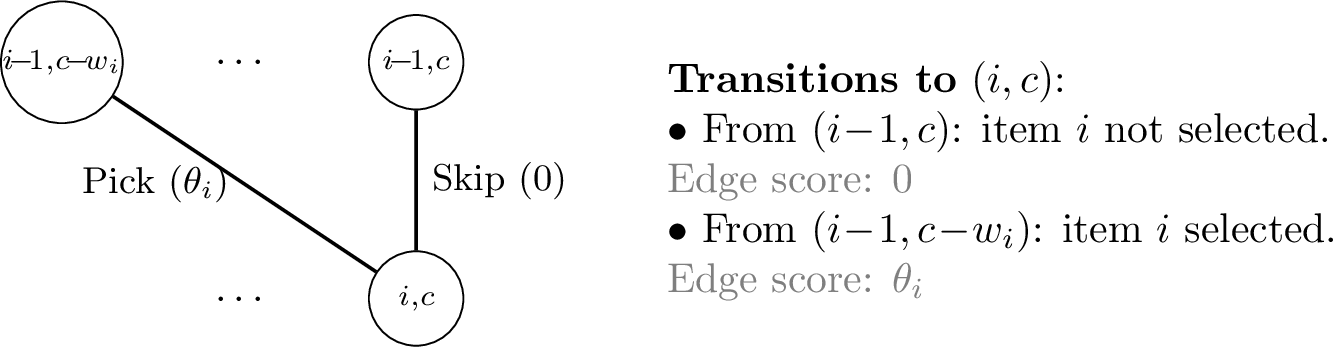
10.3.0.3 Top-\(k\) adaptation.
The Top-\(k\) problem (\({\boldsymbol{w}}=\boldsymbol{1}, C=k\)) follows the same graph topology. As explained in 3, the constraint that exactly \(k\) items must be chosen is enforced via boundary conditions of the form \(V_{(i,0)}({\boldsymbol{\Theta}}) = 0\) for all \(i\in\{0,\dots,n\}\) and \(V_{(0,j)}({\boldsymbol{\Theta}}) = -\infty\) for all \(j\in\{1,\dots,k\}\). An example showing how these boundary conditions effectively propagate and enforce the Top-\(k\) constraint is depicted in 11.
In order to formally cast this as an instance of DDP, we add artificial edges between the source node \((0,0)\) and every boundary node \((i,0)\) for \(i\in\{1,\dots,n\}\) with edge scores \({\boldsymbol{\Theta}}_{(0,0),(i,0)}=0\)., and between the source node and every node \((0,j)\) for \(j\in\{1,\dots,k\}\) with edge scores \({\boldsymbol{\Theta}}_{(0,0),(0,j)}=-\infty\)..
Under this construction, the DDP recursion exactly matches the Top-\(k\) recursion. Indeed, for \(i\in\{1,\dots,n\},j\in\{1,\dots,k\}\), we have: \[\begin{align} V_{(i,j)}({\boldsymbol{\Theta}}) &= \max\left( \underbrace{\underbrace{0}_{{\boldsymbol{\Theta}}_{(i-1,j),(i,j)}} + V_{(i-1,j)}({\boldsymbol{\Theta}})}_{\text{Skip}}, \underbrace{\underbrace{\theta_i}_{{\boldsymbol{\Theta}}_{(i-1,j-1),(i,j)}} + V_{(i-1, j-1)}({\boldsymbol{\Theta}})}_{\text{Pick}} \right),\\ V_{(i,0)}({\boldsymbol{\Theta}}) &= \max\left(\underbrace{0}_{{\boldsymbol{\Theta}}_{(0,0),(i,0)}} + V_{(0,0)}({\boldsymbol{\Theta}})\right) = V_{(0,0)}({\boldsymbol{\Theta}}) = 0,\\ V_{(0,j)}({\boldsymbol{\Theta}}) &= \max\left(\underbrace{-\infty}_{{\boldsymbol{\Theta}}_{(0,0),(0,j)}} + V_{(0,0)}({\boldsymbol{\Theta}})\right) = -\infty. \end{align}\]
11 Experimental details for 6.1↩︎
11.0.0.1 Data Generation.
We generate synthetic Knapsack instances using the genData protocol from the PyEPO library. For each instance, item weights \({\boldsymbol{w}}\in {\mathbb{N}}^n\) are sampled uniformly from the
interval \(\{3, 8\}\). The item values \({\boldsymbol{\theta}}\) are generated dependent on input features \({\boldsymbol{x}}\in {\mathbb{R}}^p\) (with \({\boldsymbol{x}}\sim \mathcal{N}(0, 1)\)) according to a polynomial relation with degree \(\text{deg}=3\): \[\begin{align} \theta_{j} = \left\lceil \left( \left(
\frac{1}{\sqrt{p}} ({\boldsymbol{B}}{\boldsymbol{x}})_j + 3 \right)^{3} + 1 \right) \cdot 5 \cdot 3.5^{-3} \cdot \epsilon_j \right\rceil,
\end{align}\] where \({\boldsymbol{B}}_{ij} \sim \text{Bernoulli}(0.5)\) and \(\epsilon_j \sim \mathcal{U}(0.7, 1.3)\) is a multiplicative noise term. The Knapsack capacity \(C\) is set to \(50\%\) of the total weight of all items: \(C\triangleq\lfloor \frac{1}{2}\sum_{i=1}^n w_i\rfloor\). We generate a total of \(18,000\) samples, split into \(10,000\) for training, \(4,000\) for validation, and \(4,000\) for testing.
11.0.0.2 Architecture and optimization.
We utilize a standard feed-forward neural network with two hidden layers of dimension \(64\) and ReLU activations. All models are trained for \(30\) epochs using the Adam optimizer with a learning rate of \(2 \times 10^{-3}\) and a batch size of \(32\). All experiments were executed on the CPU of an Apple M1 Max processor with 64 GB of RAM.
11.0.0.3 Statistical significance.
We quantify the computational overhead by measuring the wall-clock time required for a single gradient step (encompassing both forward and backward passes), averaged over \(10^4\) repetitions to mitigate variance. We monitor performance of the methods on distinct datasets generated with \(n \in \{10, 25, 50, 100\}\), each generated with the protocol described earlier. Each method is used to train a model on the training set, then the best model iteration is selected according to its relative regret on the validation set, and performance is finally reported using the relative regret on the test set. To ensure the robustness of our results, we perform a systematic evaluation across \(10\) independent random seeds for every method.
11.0.0.4 Baselines details.
We compare against the following methods provided in the PyEPO benchmark:
PFY: The perturbed Fenchel-Young loss [2], which relies on Monte-Carlo sampling of perturbed costs to estimate gradients.DBB: The differentiable black-box [4] method, which computes gradients via piecewise affine interpolation.NCE: A surrogate loss based on noise-contrastive estimation [31].NID: Treats the optimal solution mapping of combinatorial minimization problems as a negative identity function during the backward pass [32].
In order to enable a fair comparison, we use the same Numba DP-based implementation of the unregularized knapsack operator \({\boldsymbol{y}^C_{\boldsymbol{w}}}\) as a solver for every baseline.
For DBB and NID, which are differentiation methods and not loss functions, we minimize the mean squared error on solutions \(\frac{1}{2n}\|{\boldsymbol{y}^C_{\boldsymbol{w}}}(\hat{{\boldsymbol{\theta}}}^{(i)})-{\boldsymbol{y}}^{(i)}\|_2^2\).
11.0.0.5 Hyperparameters.
For the baselines and our method, we use the following hyperparameters:
DP-based Fenchel-Young losses (ours): We use a regularization strength \(\gamma=5.0\).
PFY:We use \(10\) Monte-Carlo samples and a perturbation noise \(\sigma=5.0\).DBB:We use a smoothing parameter \(\lambda=0.1\).
These hyperparameters were tuned using a grid search on the validation set.
12 Experimental details for 6.2↩︎
12.0.0.1 Problem formulation.
The agent manages a store containing \(n=20\) items over a finite horizon of \(T=80\) time steps. Each item \(i\) is assigned a static weight \(w_i\) drawn uniformly from \([5]\), a static price \(s_i>0\), and possesses a dynamic feature vector \({\boldsymbol{x}}^{(t,i)}\). At each time step \(t\), the agent selects a subset of items (an assortment) \({\boldsymbol{y}}^{(t)} \in\{0,1\}^n\) to display. This selection is subject to two operational constraints:
Knapsack constraint: the total weight of displayed items must not exceed the store’s capacity, i.e.: \[\begin{align} \sum_{i=1}^n w_i \,y^{(t)}_i \leq C\triangleq40. \end{align}\]
Inventory constraint: an item \(i\) may only be displayed if it remains in stock (\(I^{(t)}_i \geq 1\)). All items are initialized with a uniform inventory of \(I^{(0)}_i\triangleq I^{(0)}=5\).
In our precise setting, there are exactly \(|{\mathcal{Y}^C_{\boldsymbol{w}}}|=989034\) feasible assortments when every item is in stock.
12.0.0.2 Customer choice model.
Customer behavior is simulated using a multinomial logit model. Given an assortment \({\boldsymbol{y}}^{(t)}\), the customer purchases item \(i \in \{j\in[n]\mid y^{(t)}_j = 1\}\) or selects the "no-purchase" option (\(i=0\)) according to the following probabilities: \[P(i|{\boldsymbol{y}}^{(t)}) = \frac{\exp(u^{(t)}_i)}{1 + \sum_{j \in S_t} \exp(u^{(t)}_j)},\] where \(u^{(t)}_i = \langle {\boldsymbol{\phi}}, {\boldsymbol{x}}^{(t,i)} \rangle\) represents the utility of item \(i\) derived from a hidden linear customer model \({\boldsymbol{\phi}}\).
12.0.0.3 Endogenous uncertainty.
The environment features strong endogeneity in both feature evolution and state transitions. First, the inventory evolves deterministically: \(I^{(t+1)}_i = I^{(t)}_i - 1\) if item \(i\) is purchased, creating a coupling between immediate rewards and future availability. Second, item features evolve based on customer decisions. Specifically, if item \(i\) is purchased, its "satisfaction" feature (part of \({\boldsymbol{x}}^{(t,i)}\)) increases by \(1\%\). Furthermore, a "hype" feature evolves based on a rolling window of the last 5 purchases: the most recently purchased item receives a hype boost of \(+2\times10^{-2}\), while items purchased \(2\) to \(5\) steps ago suffer a decay of \(-5\times 10^{-3}\). Finally, a time feature increments linearly by \(9/T\) at each step.
12.0.0.4 State space.
The state \(s_t\) provided to the agent is a concatenation of static and dynamic information resulting in a feature dimension of \(12 \times n\). Specifically, the 12-dimensional vector \({\boldsymbol{x}}^{(t,i)}\) for item \(i\) is constructed as follows: indices \(x^{(t,i)}_0, x^{(t,i)}_1\) contain static latent attributes; \(x^{(t,i)}_2\) is the dynamic hype; \(x^{(t,i)}_3\) is the dynamic satisfaction; \(x^{(t,i)}_4\) is the static price \(\theta_i\); and \(x^{(t,i)}_5\) is the current time step. These base features are augmented by their dynamics: \(x^{(t,i)}_6,x^{(t,i)}_7\) contain the one-step difference in hype and satisfaction, while \(x^{(t,i)}_8,x^{(t,i)}_9\) contain their cumulative change since \(t=0\). Finally, \(x^{(t,i)}_{10}\) contains the normalized inventory \(I^{(t)}_i/I^{(0)}\) and \(x^{(t,i)}_{11}\) contains the normalized weight \(w_i/C\). The reward \(r_t\) is defined as the price \(s_i\) of the purchased item \(i\), or \(0\) if no purchase occurs. The objective is to maximize cumulative revenue \(\sum_{t=1}^T r_t\).
12.0.0.5 Greedy policy.
As a simple baseline, we include a greedy actor, which always displays available items that maximize the total price: \[\begin{align} {\boldsymbol{y}}^{(t)}_{\text{greedy}} \triangleq &\mathop{\mathrm{\mathsf{argmax}}}_{{\boldsymbol{y}}\in \{0,1\}^n} \;\sum_{i=1}^n s_i y_i \\ &\quad\quad\quad\quad \text{s.t.} \quad \sum_{i=1}^n w_i y_i \leq C, \\ &\quad\quad\quad\quad \text{and}\quad \forall i \in [n]\mid y_i =1,\; I^{(t)}_i \geq 1. \end{align}\] This is effectively implemented using a regular Knapsack operator, by using an artificial weights vector \(\hat{{\boldsymbol{w}}}^{(t)}\) such that \(\hat{w}^{(t)}_i=w_i\) if \(I_i^{(t)}\geq 1\), and \(\hat{w}^{(t)}_i=C+1\) if \(I_i^{(t)}=0\). We then have \({\boldsymbol{y}}^{(t)}_{\text{greedy}} = {\boldsymbol{y}}^C_{\hat{{\boldsymbol{w}}}^{(t)}}({\boldsymbol{s}})\).
12.0.0.6 Expert policy.
Finding the optimal policy is computationally intractable. We define a myopic expert policy baseline as follows at each time step \(t\), the expert computes the assortment \({\boldsymbol{y}}^{(t)}\) that maximizes the expected immediate revenue, subject to current constraints: \[\begin{align} {\boldsymbol{y}}^{(t)}_{\text{expert}} \triangleq &\mathop{\mathrm{\mathsf{argmax}}}_{{\boldsymbol{y}}\in \{0,1\}^n} \sum_{i\in[n]\mid y_i=1} s_i \cdot P(i|{\boldsymbol{y}})\\ &\quad\quad \quad\quad\quad \text{s.t.} \quad \sum_{i=1}^n w_i y_i \leq C, \\ &\quad\quad \quad\quad\quad \text{and}\quad \forall i \in [n]\mid y_i =1,\; I^{(t)}_i \geq 1. \end{align}\] To compute \({\boldsymbol{y}}^{(t)}_{\text{expert}}\), we enumerate every feasible item selection (there are \(989034\) of them in our configuration), and compute the corresponding purchase probabilities. Naturally, this baseline requires access to hidden information (the customer model \({\boldsymbol{\phi}}\) defining purchase probabilities \(P(i|{\boldsymbol{y}})\)), and is computationally costly.
12.0.0.7 SRL actors.
The actors in the SRL-based methods are paramterized by a feed-forward neural network \(f_{W_1}\) mapping states \({\boldsymbol{x}}^{(t)}\in{\mathbb{R}}^{12\times n}\) to item logits \(\hat{{\boldsymbol{\theta}}}\in{\mathbb{R}}^{^n}\), which are then mapped to feasible assortments by the hard Knapsack operator \({\boldsymbol{y}}^C_{\hat{{\boldsymbol{w}}}^{(t)}}(\hat{{\boldsymbol{\theta}}})\), where \(\hat{w}^{(t)}_i=w_i\) if \(I_i^{(t)}\geq 1\), and \(\hat{w}^{(t)}_i=C+1\) if \(I_i^{(t)}=0\) (effectively enforcing the inventory constraint).
12.0.0.8 Exploration and gradient computation.
In standard SRL [35], \(K\) exploration targets are generated by perturbing the predicted logits \(\hat{{\boldsymbol{\theta}}}\) with a random variable \(Z\) (which follows, e.g., a centered Gaussian distribution in \({\mathbb{R}}^n\)) to get samples: \[\begin{align} {\boldsymbol{y}}^{(k)}\triangleq {\boldsymbol{y}}^C_{\hat{{\boldsymbol{w}}}^{(t)}}(\hat{{\boldsymbol{\theta}}} + \varepsilon Z^{(k)})\in {\mathcal{Y}}^C_{\hat{{\boldsymbol{w}}}^{(t)}}\;, \end{align}\]
where \(\varepsilon>0\) is a hyperparameter and the \(Z^{(k)}\) are i.i.d. samples. Then, the target \(\hat{{\boldsymbol{y}}}\) is defined by aggregating these samples via a softmax operation using Q-values predicted by a critic network \(\psi_{W_2}\): \[\begin{align} \hat{{\boldsymbol{y}}}\triangleq \sum_{k=1}^K\frac{\exp\left(\frac{\psi_{W_2}({\boldsymbol{x}}, {\boldsymbol{y}}^{(k)})}{\tau}\right)}{\sum_{k'=1}^K \exp\left(\frac{\psi_{W_2}({\boldsymbol{x}}, {\boldsymbol{y}}^{(k')})}{\tau}\right)}\cdot {\boldsymbol{y}}^{(k)}\in {\mathsf{conv}}\left({\mathcal{Y}}^C_{\hat{{\boldsymbol{w}}}^{(t)}}\right). \end{align}\] Finally, a perturbation-based Fenchel-Young loss [2] is used to compute gradients with respect to \(\hat{{\boldsymbol{\theta}}}\), which are then backpropagated to upstream weights \(W_1\). This gradient is estimated via Monte-Carlo as: \[\begin{align} \nabla_{\boldsymbol{\theta}}L_\varepsilon(\hat{{\boldsymbol{\theta}}}\,;\hat{{\boldsymbol{y}}}) \approx \frac{1}{M}\sum_{m=1}^M {\boldsymbol{y}}^C_{\hat{{\boldsymbol{w}}}^{(t)}}(\hat{{\boldsymbol{\theta}}} + \varepsilon Z^{(m)}) - \hat{{\boldsymbol{y}}}, \end{align}\] where the \(Z^{(m)}\) are again i.i.d. samples.
What we propose for our DP-based SRL agents instead, is to use 4 to produce \(K\) exploration actions: \[\begin{align} {\boldsymbol{y}}^{(k)}\sim \pi^{\hat{{\boldsymbol{w}}}^{(t)},C}_{\hat{{\boldsymbol{\theta}}},\Omega}\in {\mathcal{Y}}^C_{\hat{{\boldsymbol{w}}}^{(t)}}\;, \end{align}\] and to use our DP-based Fenchel-Young losses to compute exact gradients \[\begin{align} \nabla_{\boldsymbol{\theta}}L_{\Omega^C_{\hat{{\boldsymbol{w}}}^{(t)}}}(\hat{{\boldsymbol{\theta}}}\,;\hat{{\boldsymbol{y}}}) = {\boldsymbol{y}}^C_{\hat{{\boldsymbol{w}}}^{(t)},\Omega} - \hat{{\boldsymbol{y}}}, \end{align}\] using 3. Importantly, we only need to call 2 once to produce intermediate outputs for 3 4, yielding computational gains.
12.0.0.9 PPO Baseline.
We adapt proximal policy optimization (PPO) [36] to the combinatorial setting following the COaML-pipeline framework detailed in [35]. In this formulation, the PPO agent does not directly output discrete actions. Instead, the actor network \(f_{W_1}\) predicts a latent score vector \(\hat{{\boldsymbol{\theta}}} \in {\mathbb{R}}^n\), which parameterizes a multivariate Gaussian policy \(\pi_{\hat{{\boldsymbol{\theta}}}}({\boldsymbol{\eta}}) = {\mathcal{N}}({\boldsymbol{\eta}}\mid \hat{{\boldsymbol{\theta}}}, \sigma^2 {\boldsymbol{I}})\). During the rollout, a continuous score vector \({\boldsymbol{\eta}}\) is sampled from this distribution and passed to the hard Knapsack solver to produce the discrete item selection \({\boldsymbol{y}}^{(t)} = {\boldsymbol{y}}^C_{\hat{{\boldsymbol{w}}}^{(t)}}({\boldsymbol{\eta}})\). From the perspective of the PPO algorithm, the actor’s action is the sampled continuous vector \({\boldsymbol{\eta}}\), the combinatorial solver is treated as a deterministic transition function within the environment dynamics, and the optimization objective is to adjust the mean \(\hat{{\boldsymbol{\theta}}}\) of the score distribution to maximize returns. The policy ratio and clipping are computed on the continuous densities of the perturbed scores \({\boldsymbol{\eta}}\). We anneal the exploration standard deviation \(\sigma\) linearly during training.
12.0.0.10 Hyperparameters.
We train all agents for \(10^4\) episodes, performing \(10\) update iterations with a batch size of \(32\) at the end of each episode for SRL, and \(100\) iterations for PPO to compensate for its on-policy data efficiency. We maintain a replay buffer with a capacity of \(10^4\) transitions and use the Adam optimizer with a learning rate of \(8 \times 10^{-5}\) for all networks. For the SRL agents, we set the perturbation noise scale \(\varepsilon\) and the regularization strength \(\gamma\) to the same value, annealing it linearly from \(5.0\) to \(1.0\) over the course of training. We use \(K=32\) exploration samples for target action creation, and the softmax aggregation temperature \(\tau\) is annealed linearly from \(1.0\) to \(0.5\). For PPO, we use a clipping ratio of \(\epsilon=0.2\), and the exploration standard deviation \(\sigma\) is annealed linearly from \(2.0\) to \(1.0\). All experiments were executed on the CPU of an Apple M1 Max processor with 64 GB of RAM.
13 Experimental details for 6.3↩︎
13.0.0.1 Derivation of the FY-DVAE Objective.
Standard DVAEs maximize the ELBO: \[\begin{align} \log p_{W_2}({\boldsymbol{x}}) \geq {\mathbb{E}}_{Y\sim q_{W_1}(\cdot\mid {\boldsymbol{x}})}[\log p_{W_2}({\boldsymbol{x}}\mid Y)] - D_{\text{KL}}(q_{W_1}(\cdot\mid {\boldsymbol{x}}) \mid\mid p(\cdot)). \end{align}\] In the standard setting DVAE setting of, e.g., [21], where the approximate posterior is parameterized as a Gibbs distribution \(q_{W_1}({\boldsymbol{y}}|{\boldsymbol{x}}) = \pi_{{\boldsymbol{\theta}}}({\boldsymbol{y}}) \propto \exp(\langle {\boldsymbol{\theta}}, {\boldsymbol{y}}\rangle)\) with \({\boldsymbol{\theta}}=E_{W_1}({\boldsymbol{x}})\), and the prior \(p\) is the uniform distribution on \(k\)-subsets \(p\propto 0\), the KL divergence regularization term writes: \[\begin{align} D_{\text{KL}}(\pi_{\boldsymbol{\theta}}\mid\mid p) &\triangleq \sum_{{\boldsymbol{y}}\in{\mathcal{Y}^k_{\boldsymbol{1}}}}\pi_{\boldsymbol{\theta}}({\boldsymbol{y}})\log\left(\frac{\pi_{\boldsymbol{\theta}}({\boldsymbol{y}})}{p({\boldsymbol{y}})}\right)\\ &= - \sum_{{\boldsymbol{y}}\in{\mathcal{Y}^k_{\boldsymbol{1}}}}\pi_{\boldsymbol{\theta}}({\boldsymbol{y}})\log\left(\frac{1}{|{\mathcal{Y}^k_{\boldsymbol{1}}}|}\right) + \sum_{{\boldsymbol{y}}\in{\mathcal{Y}^k_{\boldsymbol{1}}}}\pi_{\boldsymbol{\theta}}({\boldsymbol{y}})\log\left(\pi_{\boldsymbol{\theta}}({\boldsymbol{y}})\right) \\ &= \log\left(|{\mathcal{Y}^k_{\boldsymbol{1}}}|\right) + \sum_{{\boldsymbol{y}}\in{\mathcal{Y}^k_{\boldsymbol{1}}}}\frac{\exp(\langle{\boldsymbol{\theta}},{\boldsymbol{y}}\rangle)}{\sum_{{\boldsymbol{y}}'\in{\mathcal{Y}^k_{\boldsymbol{1}}}}\exp(\langle{\boldsymbol{\theta}},{\boldsymbol{y}}'\rangle)}\left(\langle{\boldsymbol{\theta}},{\boldsymbol{y}}\rangle - \log\sum_{{\boldsymbol{y}}'\in{\mathcal{Y}^k_{\boldsymbol{1}}}}\exp(\langle{\boldsymbol{\theta}},{\boldsymbol{y}}'\rangle)\right)\\ &= \log\left(|{\mathcal{Y}^k_{\boldsymbol{1}}}|\right) - \log\sum_{{\boldsymbol{y}}'\in{\mathcal{Y}^k_{\boldsymbol{1}}}}\exp(\langle{\boldsymbol{\theta}},{\boldsymbol{y}}'\rangle) + \left\langle \sum_{{\boldsymbol{y}}\in{\mathcal{Y}^k_{\boldsymbol{1}}}}\frac{\exp(\langle{\boldsymbol{\theta}},{\boldsymbol{y}}\rangle)}{\sum_{{\boldsymbol{y}}'\in{\mathcal{Y}^k_{\boldsymbol{1}}}}\exp(\langle{\boldsymbol{\theta}},{\boldsymbol{y}}'\rangle)}{\boldsymbol{y}},\;{\boldsymbol{\theta}}\right\rangle\\ &= A(\boldsymbol{0}) - A({\boldsymbol{\theta}}) + \langle\nabla A({\boldsymbol{\theta}}) ,{\boldsymbol{\theta}}\rangle, \end{align}\] where \(A({\boldsymbol{\theta}}) = \log \sum_{{\boldsymbol{y}}\in{\mathcal{Y}^k_{\boldsymbol{1}}}} \exp(\langle {\boldsymbol{\theta}}, {\boldsymbol{y}}\rangle)\) is the cumulant function of \(\pi_{\boldsymbol{\theta}}\). We recognize this expression as a Fenchel-Young loss generated by the convex conjugate of the cumulant, \(A^*\). Indeed, we have: \[\begin{align} L_{A^*}(\boldsymbol{0}\,; \nabla A({\boldsymbol{\theta}})) &\triangleq A^{**}(\boldsymbol{0}) + A^*(\nabla A({\boldsymbol{\theta}})) - \langle \boldsymbol{0}, \nabla A({\boldsymbol{\theta}}) \rangle \quad \text{\cite{blondel_learning_2020}} \\ &= A(\boldsymbol{0}) + (\langle {\boldsymbol{\theta}}, \nabla A({\boldsymbol{\theta}}) \rangle - A({\boldsymbol{\theta}})) \quad \text{(A^{**}=A and Fenchel's equality)} \\ &= A(\boldsymbol{0}) - A({\boldsymbol{\theta}}) + \langle {\boldsymbol{\theta}}, \nabla A({\boldsymbol{\theta}}) \rangle \\ &= D_{\text{KL}}(\pi_{\boldsymbol{\theta}}\mid\mid p). \end{align}\] Here, we used the fact that \(A\) is convex and lower semi-continuous to apply the Fenchel-Moreau biconjugation theorem, and Fenchel’s equality \(A^*(\nabla A({\boldsymbol{\theta}})) + A({\boldsymbol{\theta}}) = \langle {\boldsymbol{\theta}}, \nabla A({\boldsymbol{\theta}}) \rangle\).
We generalize this to our smoothed DP setting by using a generalized approximate posterior \(q_{W_1}({\boldsymbol{y}}|{\boldsymbol{x}})=\pi^{\boldsymbol{1},k}_{\boldsymbol{\theta},\Omega}({\boldsymbol{y}})\), and by replacing \(A^*\) with the generalized moment polytope regularization function \({\Omega^k_{\boldsymbol{1}}}\), defined in 5.3 as the conjugate of the smoothed value \(\mathsf{max}^k_{\boldsymbol{1},\Omega}\). The resulting regularization term is the Fenchel-Young loss between the uniform prior parameters \(\boldsymbol{0}\) and the relaxed item selection \(\boldsymbol{y}^k_{\boldsymbol{1},\Omega}({\boldsymbol{\theta}})\): \[\begin{align} L_{{\Omega^k_{\boldsymbol{1}}}}(\boldsymbol{0}\,; \boldsymbol{y}^k_{\boldsymbol{1},\Omega}({\boldsymbol{\theta}})) &\triangleq ({\Omega^k_{\boldsymbol{1}}})^*(\boldsymbol{0}) + {\Omega^k_{\boldsymbol{1}}}(\boldsymbol{y}^k_{\boldsymbol{1},\Omega}({\boldsymbol{\theta}})) - \langle \boldsymbol{0}, \boldsymbol{y}^k_{\boldsymbol{1},\Omega}({\boldsymbol{\theta}}) \rangle \\ &= (\langle {\boldsymbol{\theta}}, \boldsymbol{y}^k_{\boldsymbol{1},\Omega}({\boldsymbol{\theta}}) \rangle - \mathsf{max}^k_{\boldsymbol{1},\Omega}({\boldsymbol{\theta}})) + \mathsf{max}^k_{\boldsymbol{1},\Omega}(\boldsymbol{0}) \\ &= \mathsf{max}^k_{\boldsymbol{1},\Omega}(\boldsymbol{0}) - \mathsf{max}^k_{\boldsymbol{1},\Omega}({\boldsymbol{\theta}}) + \langle {\boldsymbol{\theta}}, \boldsymbol{y}^k_{\boldsymbol{1},\Omega}({\boldsymbol{\theta}}) \rangle. \end{align}\] By construction, as \(\Omega=-H^s\) yields \(\mathsf{max}^k_{\boldsymbol{1},\Omega}=A\) and \(\pi^{\boldsymbol{1},k}_{\boldsymbol{\theta},\Omega}=\pi_{\boldsymbol{\theta}}\) (see [sec:properties] [prop:distribution]), this formulation recovers the standard KL divergence objective used in [21] as a special case, while enabling the use of regularizers that incentivize sparse latent representations (e.g., Gini or \(1.5\)-Tsallis). This framework also extends the Fenchel-Young variational inference framework of [38], which introduced Fenchel-Young regularization for learning continuous VAEs, to the discrete setting of latent distributions on \(k\)-subsets. Moreover, the gradient of this Fenchel-Young regularization term is given by: \[\begin{align} \nabla_{\boldsymbol{\theta}}L_{{\Omega^k_{\boldsymbol{1}}}}(\boldsymbol{0}\,; \boldsymbol{y}^k_{\boldsymbol{1},\Omega}({\boldsymbol{\theta}})) = (\nabla_{\boldsymbol{\theta}}\boldsymbol{y}^k_{\boldsymbol{1},\Omega}({\boldsymbol{\theta}}))\cdot{\boldsymbol{\theta}}, \end{align}\] that is, it is simply the JVP of the relaxed layer \(\boldsymbol{y}^k_{\boldsymbol{1},\Omega}\) in the direction of its input \({\boldsymbol{\theta}}\), efficiently computed via 9.
13.0.0.2 Dataset Generation.
We construct each data point in our Stacked MNIST dataset by sampling \(k=3\) distinct digit classes \(\{c_1, \dots, c_k\} \subset \{0, \dots, 9\}\) without replacement. For each class \(c_j\), we sample a random image \({\boldsymbol{x}}^{(j)}\) from the standard MNIST dataset. The input \({\boldsymbol{x}}\) is the pixel-wise average: \({\boldsymbol{x}}= \frac{1}{k} \sum_{j=1}^k {\boldsymbol{x}}^{(j)}\). The ground truth is the \(k\)-hot vector \({\boldsymbol{y}}\in \{0,1\}^{10}\) indicating the present digits. We generate \(120,000\) training examples and \(20,000\) test examples.
13.0.0.3 Architecture.
The model architecture captures both the presence and the style of the digits using a decomposed latent space with dimensions \(n=10\) for the discrete part and \(d_z=32\) for the continuous part. The encoder \(E_{W_1}\) is a convolutional neural network consisting of a stack of strided convolution layers (kernel size \(3\times3\), stride \(2\), ReLU activation), which progressively downsample the spatial dimensions while increasing channel depth. The resulting flattened feature map is fed into two separate dense projection heads: one outputting the selection logits \(\hat{{\boldsymbol{\theta}}} \in {\mathbb{R}}^{10}\) for the discrete mask \({\boldsymbol{y}}\), and another outputting the parameters \([{\boldsymbol{\mu}}, \log{\boldsymbol{\sigma}}^2] \in {\mathbb{R}}^{10 \times 2d_z}\) for the \(n=10\) independent Gaussian style posteriors \({\boldsymbol{z}}_i \sim {\mathcal{N}}({\boldsymbol{\mu}}_i, \text{diag}({\boldsymbol{\sigma}}_i^2))\).
The mapping from selection logits \(\hat{{\boldsymbol{\theta}}}\) to mixing coefficients \({\boldsymbol{y}}\) in the discrete bottleneck depends on the considered method:
for the hard Top-\(k\) baseline, the mapping is simply \({\boldsymbol{y}}={\boldsymbol{y}^k_{\boldsymbol{1}}}({\boldsymbol{\theta}})\in{\mathcal{Y}^k_{\boldsymbol{1}}}\),
for the Gumbel Top-\(k\) baseline, we sample i.i.d. Gumbel noise \(Z_i\sim \text{Gumbel}(0,1)\) for \(i\in[10]\) and take the Top-\(k\) of the perturbed values \({\boldsymbol{y}}={\boldsymbol{y}^k_{\boldsymbol{1}}}({\boldsymbol{\theta}}+ \tau {\boldsymbol{Z}})\in{\mathcal{Y}^k_{\boldsymbol{1}}}\),
for our deterministic DP-based layers, we directly use the relaxed Top-\(k\) operator \({\boldsymbol{y}}=\boldsymbol{y}^k_{\boldsymbol{1},\Omega}({\boldsymbol{\theta}})\in{\mathsf{conv}}({\mathcal{Y}^k_{\boldsymbol{1}}})\) using 3,
and for our stochastic DP-based layers, we sample from the underlying distribution via \({\boldsymbol{y}}\sim\pi^{\boldsymbol{1},k}_{\boldsymbol{\theta},\Omega}\) using 4.
We maintain a set of learned embeddings \(\mathbf{E} = \{{\boldsymbol{e}}_1, \dots, {\boldsymbol{e}}_{10}\}\) with \({\boldsymbol{e}}_i \in {\mathbb{R}}^{d_z}\), representing the prototypes for each digit class. The decoder \(D_{W_2}\) is a shared de-convolutional network applied independently to each expert. For each item \(i\), it receives the concatenation \([{\boldsymbol{z}}_i, {\boldsymbol{e}}_i] \in {\mathbb{R}}^{2 d_z}\) of the sampled style code and the prototype embedding. This input is mapped via a dense layer to a low-resolution feature map, then upsampled via a stack of transposed convolution layers (kernel size \(3\times3\), stride \(2\), ReLU activation) to reach the target image resolution. A final convolution layer followed by a sigmoid activation produces the candidate reconstruction \(\hat{{\boldsymbol{x}}}_i \in [0,1]^{H \times W}\). The final output is the weighted average of these candidates: \[\begin{align} \hat{{\boldsymbol{x}}} = \frac{1}{k} \sum_{i=1}^{10} y_i \cdot \sigma\left( D_{W_2}([{\boldsymbol{z}}_i, {\boldsymbol{e}}_i]) \right) = \frac{1}{k} \sum_{i=1}^{10} y_i \cdot \hat{{\boldsymbol{x}}}_i. \end{align}\]
13.0.0.4 Training Details.
The models are trained using the Adam optimizer with a learning rate of \(3 \times 10^{-4}\) and a batch size of \(64\) for \(50\) epochs. The full training objective is given by: \[\begin{align} {\mathcal{L}}({\boldsymbol{x}}\,; W_1, W_2) =\; &\|{\boldsymbol{x}}- \hat{{\boldsymbol{x}}}\|_2^2 + \beta_{\text{KL}} \sum_{i=1}^{10} D_{\text{KL}}({\mathcal{N}}({\boldsymbol{\mu}}_i, \text{diag}({\boldsymbol{\sigma}}_i^2)) || {\mathcal{N}}(\boldsymbol{0}, {\boldsymbol{I}})) + \beta_{\text{FY}} \cdot L_{{\Omega^k_{\boldsymbol{1}}}}(\boldsymbol{0}\,; \boldsymbol{y}^k_{\boldsymbol{1},\Omega}(\hat{{\boldsymbol{\theta}}})). \end{align}\] We use a fixed weight \(\beta_{\text{KL}}=10^{-5}\) for the continuous latent regularization. We anneal the discrete Fenchel-Young regularization strength \(\beta_{\text{FY}}\) linearly from \(0\) to a base value of \(10^{-5}\) over the first two-thirds of the training epochs. All displayed metrics are averaged over \(30\) trainings with different random seeds. All experiments were executed on TPUv2 with one device.
13.1 Properties of the relaxed values and operators↩︎
The relaxed values and operators have the following properties:
The smoothed output values \({\boldsymbol{\theta}}\mapsto\mathsf{max}^C_{\boldsymbol{w},\Omega}({\boldsymbol{\theta}})\) and \({\boldsymbol{\theta}}\mapsto\mathsf{max}^k_{\boldsymbol{1},\Omega}({\boldsymbol{\theta}})\) are convex in \({\boldsymbol{\theta}}\).
Define \(\Omega_d:\triangle^{d}\to{\mathbb{R}}\) as \(\Omega_d({\boldsymbol{q}})\triangleq \sum_{i=1}^d\omega(q_i)\) for any integer \(d\). Then, the difference between the smoothed and the unregularized values are bounded above and below, for all \({\boldsymbol{\theta}}\in{\mathbb{R}}^n\): \[\begin{align} (N_C-1)L_{N_C}&\leq {\mathsf{max}^C_{\boldsymbol{w}}}({\boldsymbol{\theta}})-\mathsf{max}^C_{{\boldsymbol{w}},\Omega_2}({\boldsymbol{\theta}})\leq (N_C-1)U_{N_C},\\ (N_k-1)L_{N_k}&\leq {\mathsf{max}^k_{\boldsymbol{1}}}({\boldsymbol{\theta}})-\mathsf{max}^k_{\boldsymbol{1},\Omega_2}({\boldsymbol{\theta}})\leq (N_k-1)U_{N_k}, \end{align}\] where \(L_d\) and \(U_d\) are lower and upper bounds of \(\Omega_d\) on \(\triangle^d\), and with \(N_C\triangleq (C+1)(n+1)\), \(N_k\triangleq(k+1)(n+1)\).
The proposed layers converge to the original, hard operators for vanishing regularization: \[\begin{align} {\boldsymbol{y}}_{{\boldsymbol{w}},\,\gamma\Omega}^C\xrightarrow[\gamma\to0^+]{}{\boldsymbol{y}^C_{\boldsymbol{w}}}({\boldsymbol{\theta}}),\quad {\boldsymbol{y}}_{\boldsymbol{1},\,\gamma\Omega}^k\xrightarrow[\gamma\to0^+]{}{\boldsymbol{y}^k_{\boldsymbol{1}}}({\boldsymbol{\theta}}). \end{align}\]
Proof. These properties stem from a direct application of results in [7] to our special DAG and edge weights, after mapping our framework to the DDP framework as described in 10.3. The constants \(N_C\) and \(N_k\) emerge from the size of the corresponding DAG. ◻
14 Explicit derivations↩︎
In this section, we provide explicit derivations for the quantities \(Q^{\boldsymbol{w}}_{\Omega}[i,c]\) and their partial derivatives used in the algorithms. Recall the definition of the smoothed value function \(V^{\boldsymbol{w}}_{\Omega}[i,c]\) from 4 :
\[\begin{align} &V^{\boldsymbol{w}}_{\Omega}[i,c] \triangleq \begin{cases} V^{\boldsymbol{w}}_{\Omega}[i-1, c] &\text{if w_{i}>c,}\\[5pt] \mathsf{max}_\Omega\bigl(\theta_{i}+V^{\boldsymbol{w}}_{\Omega}[i-1, c-w_{i}],\;V^{\boldsymbol{w}}_{\Omega}[i-1, c]\bigr) &\text{else.} \end{cases} \end{align}\]
We focus on the non-trivial case where \(w_i \le c\). We define the local inputs \(a\) and \(b\) as: \[\begin{align} a &\triangleq \theta_i + V^{\boldsymbol{w}}_{\Omega}[i-1, c-w_i], \\ b &\triangleq V^{\boldsymbol{w}}_{\Omega}[i-1, c]. \end{align}\] The smoothed maximum is defined as the optimal value of the regularized objective: \[\begin{align} \mathsf{max}_\Omega(a, b) \triangleq \max_{q \in [0,1]} J(q\,; a, b), \quad \text{where } J(q\,; a, b) \triangleq q a + (1-q) b - \Omega({\boldsymbol{q}}). \end{align}\] Here, \({\boldsymbol{q}}= (q, 1-q)^\top\) and \(\Omega({\boldsymbol{q}}) = \omega(q) + \omega(1-q)\) is a separable strictly convex regularization function. We denote the unique maximizer by \(q^*(a, b)\). The partial derivatives required for the algorithms are given by Danskin’s theorem and the chain rule: \[\begin{align} Q^{\boldsymbol{w}}_{\Omega}[i,c] &= q^*(a,b), \\ \frac{\partial Q^{\boldsymbol{w}}_{\Omega}[i,c]}{\partial \theta_i} &= \frac{\partial q^*}{\partial a}(a, b). \end{align}\] In the following, we derive \(q^*\) and \(\frac{\partial q^*}{\partial a}\) for specific choices of \(\Omega\). The resulting explicit expressions are summarized in ¿tbl:tab:instantiations?, together with the corresponding expression of \(V^{\boldsymbol{w}}_{\Omega}[i,c]=\mathsf{max}_\Omega(a,b)=J(q^*(a,b)\,;a,b)\).
14.1 General derivative computation↩︎
The optimization problem \(\max_{q \in [0,1]} J(q\,; a, b)\) is equivalent to the minimization problem: \[\begin{align} \min_{q \in {\mathbb{R}}} \quad & \Phi(q) \triangleq \omega(q) + \omega(1-q) - q a - (1-q) b \\ \text{s.t.} \quad & g_1(q) \triangleq -q \le 0, \nonumber \\ & g_2(q) \triangleq q - 1 \le 0. \nonumber \end{align}\] Let \(\mu, \lambda \ge 0\) be the KKT multipliers associated with \(g_1\) and \(g_2\) respectively. The KKT stationarity condition necessitates: \[\begin{align} \label{eq:general95stationarity} \omega'(q^*) - \omega'(1-q^*) - (a-b) - \mu + \lambda = 0. \end{align}\tag{14}\]
We now distinguish two regimes for the sensitivity \(\frac{\partial q^*}{\partial a}\).
14.1.0.1 Case 1: interior solution.
Assume the optimal solution lies in the strict interior \(q^* \in (0,1)\). The box constraints are inactive and we have \(\mu = \lambda = 0\). The stationarity condition 14 simplifies to: \[\begin{align} w'(q^*)-w'(1-q^*) = a - b. \end{align}\] Differentiating with respect to \(a\) yields: \[\begin{align} \label{eq:partial95stationarity} \frac{\partial q^*}{\partial a} = \frac{1}{w''(q^*)+w''(1-q^*)}. \end{align}\tag{15}\]
14.1.0.2 Case 2: boundary solution.
We now consider the case where the solution saturates at a boundary. This occurs if and only if the regularizer has bounded gradients at the endpoints. Assume \(\lim_{q \to 1^-} \omega'(q) = L < \infty\) and \(\lim_{q \to 0^+} \omega'(q) = l > -\infty\). Let \(\tau_\Omega \triangleq L - l\). We prove that if \(a-b \ge \tau_\Omega\), then \(q^*=1\) and \(\frac{\partial q^*}{\partial a} = 0\).
Let \(q^*=1\). The active constraint is \(g_2(q) \le 0\), so \(\mu=0\) and \(\lambda \ge 0\). The stationarity condition 14 becomes: \[\begin{align} \lambda &= (a-b) - (\omega'(1) - \omega'(0)) \\ &= (a-b) - \tau_\Omega. \end{align}\] Dual feasibility requires \(\lambda \ge 0\), which holds if and only if \(a-b \ge \tau_\Omega\). Since the problem is strictly convex, the KKT conditions are sufficient for optimality. Thus, for all \((a,b)\) such that \(a-b > \tau_\Omega\), the unique minimizer is \(q^*=1\). In this open region, \(q^*\) is constant with respect to \(a\), implying: \[\begin{align} \frac{\partial q^*}{\partial a} = 0. \end{align}\] A symmetric argument shows that if \(a-b \le -\tau_\Omega\), then \(q^*=0\) and the derivative is zero.
14.2 Shannon entropy↩︎
We consider \(\Omega({\boldsymbol{q}}) = -\gamma H^s({\boldsymbol{q}}) \triangleq \gamma \sum_{i=1}^2q_i\log q_i\), which implies \(\omega(q) = \gamma q \log q\). The gradients of \(\omega\) become unbounded at the boundaries (\(\lim_{q\to 0} \omega'(q) = -\infty\)), forcing the solution to be strictly interior for any \(a, b\in{\mathbb{R}}\).
14.2.0.1 Maximizer.
The stationarity condition 14 yields: \[\begin{align} \gamma \log q^* - \gamma \log(1-q^*) = a-b \iff \gamma \log \left(\frac{q^*}{1-q^*}\right) = a-b. \end{align}\] Solving for \(q^*\) yields the logistic function \(q^* = \sigma(\frac{a-b}{\gamma})\triangleq (1+\exp((b-a)/\gamma))^{-1}\).
14.2.0.2 Partial derivative.
The derivative is computed via 15 derived in Case 1: \[\begin{align} \frac{\partial q^*}{\partial a} = \frac{1}{\omega''(q^*) + \omega''(1-q^*)} = \left( \frac{\gamma}{q^*} + \frac{\gamma}{1-q^*} \right)^{-1} = \frac{q^*(1-q^*)}{\gamma}. \end{align}\]
14.2.0.3 Smoothed maximum.
Substituting the optimal probability \(q^*\) back into the objective function \(J\) yields the standard log-sum-exp as expected: \[\begin{align} \mathsf{max}_\Omega(a,b) = \gamma \log \left( \exp(a/\gamma) + \exp(b/\gamma) \right). \end{align}\]
14.3 Gini entropy↩︎
We consider \(\Omega({\boldsymbol{q}}) = -\gamma H^g({\boldsymbol{q}}) \triangleq \frac{\gamma}{2} (\|{\boldsymbol{q}}\|_2^2 - 1)\), which implies \(\omega(q) = \frac{\gamma}{2} q^2 - \frac{\gamma}{4}\).
14.3.0.1 Maximizer.
In this case, we have: \[\begin{align} \omega'(q) - \omega'(1-q) = \gamma q - \gamma(1-q) = 2\gamma q - \gamma, \end{align}\] so that 14 becomes: \[\begin{align} 2\gamma q^* - \gamma - (a-b) - \mu + \lambda = 0 \implies q^* = \frac{a-b+\gamma + \mu - \lambda}{2\gamma}. \end{align}\] We analyze the solution based on the active constraints using the complementary slackness conditions \(\mu q^* = 0\) and \(\lambda (q^* - 1) = 0\).
Inactive constraints (\(\mu=0, \lambda=0\)): we have \(q^* = \frac{a-b+\gamma}{2\gamma}\). Primal feasibility \(0 < q^* < 1\) requires \(0 < \frac{a-b+\gamma}{2\gamma} < 1\), which simplifies to \(-\gamma < a-b < \gamma\). In this region, \(\frac{\partial q^*}{\partial a} = \frac{1}{2\gamma}\).
Active lower bound (\(q^*=0\)): we have \(\lambda = 0\) and \(\mu \ge 0\). The stationarity condition yields \(0 = \frac{a-b+\gamma + \mu}{2\gamma}\), which implies \(\mu = -(a-b+\gamma)\). Dual feasibility \(\mu \ge 0\) requires \(a-b+\gamma \le 0 \iff a-b \le -\gamma\). In this region, \(q^*\) is constant, so \(\frac{\partial q^*}{\partial a} = 0\).
Active upper bound (\(q^*=1\)): we have \(\mu = 0\) and \(\lambda \ge 0\). The stationarity condition yields \(1 = \frac{a-b+\gamma - \lambda}{2\gamma}\), which implies \(2\gamma = a-b+\gamma - \lambda\), or \(\lambda = a-b-\gamma\). Dual feasibility \(\lambda \ge 0\) requires \(a-b-\gamma \ge 0 \iff a-b \ge \gamma\). In this region, \(q^*\) is constant, so \(\frac{\partial q^*}{\partial a} = 0\).
Combining these three cases, we recover the projection onto \([0,1]\): \[\begin{align} q^* = \mathop{\mathrm{{\mathsf{clip}}}}_{[0,1]}\left( \frac{a-b+\gamma}{2\gamma} \right). \end{align}\]
14.3.0.2 Partial derivative.
The partial derivative is constant and only non-zero on the non-clipped region: \[\begin{align} \frac{\partial q^*}{\partial a} = \frac{1}{2\gamma} \cdot \mathbb{1}_{\{|a-b| < \gamma\}}. \end{align}\]
14.3.0.3 Smoothed maximum.
The regularization term simplifies to \(\Omega({\boldsymbol{q}}) = \gamma(q^2 - q)\) for any \({\boldsymbol{q}}=(q,(1-q))^\top\). Substituting the optimal \(q^*\) into the objective function \(J\) yields: \[\begin{align} \mathsf{max}_\Omega(a,b) = q^* a + (1-q^*) b - \gamma((q^*)^2 - q^*). \end{align}\] When saturation occurs (i.e., \(|a-b| \ge \gamma\)), we have \(q^* \in \{0, 1\}\). In this case, the regularization term vanishes and we recover the hard maximum \(\max(a,b)\). In the interior region (i.e., \(|a-b| < \gamma\)), substituting \(q^* = \frac{a-b+\gamma}{2\gamma}\) yields the following quadratic form: \[\begin{align} \mathsf{max}_\Omega(a,b) = \frac{(a-b)^2}{4\gamma} + \frac{a+b}{2} + \frac{\gamma}{4}. \end{align}\]
14.4 1.5-Tsallis Entropy↩︎
We consider \(\Omega({\boldsymbol{q}}) = -\gamma H_{1.5}^T({\boldsymbol{q}}) \triangleq \gamma\sum_{i=1}^2\frac{q_i^{\frac{3}{2}}-q_i}{\frac{3}{2}(\frac{3}{2}-1)}\), which implies \(\omega(q) = \frac{4\gamma}{3} q^{\frac{3}{2}} - \frac{2\gamma}{3}\) and \(\omega'(q) = 2\gamma \sqrt{q}\).
14.4.0.1 Maximizer.
The stationarity condition for an interior solution (\(q^* \in (0,1)\)) requires: \[\begin{align} 2\gamma\sqrt{q^*} - 2\gamma\sqrt{1-q^*} = a-b. \end{align}\] Let \(C \triangleq \frac{a-b}{2\gamma}\). We seek to solve \(\sqrt{q^*} - \sqrt{1-q^*} = C\). The function \(f(q) = \sqrt{q} - \sqrt{1-q}\) is strictly increasing on \([0,1]\) with range \([-1, 1]\).
If \(|C| > 1\) (i.e., \(|a-b| > 2\gamma\)), no interior solution exists. The monotonicity of the objective forces the solution to the boundary: \(q^*=1\) if \(C > 1\), and \(q^*=0\) if \(C < -1\).
If \(|C| \le 1\), we square the stationarity equation: \(q^* - 2\sqrt{q^*(1-q^*)} + (1-q^*) = C^2\), which rearranges to \(2\sqrt{q^*(1-q^*)} = 1 - C^2\). Squaring again yields the quadratic equation \(4(q^*)^2 - 4q^* + (1 - C^2)^2 = 0\). The roots are \(q_{\pm} = \frac{1 \pm |C|\sqrt{2 - C^2}}{2}\). To satisfy the sign of the original equation \(\sqrt{q^*} - \sqrt{1-q^*} = C\), we must select the root such that \(\mathrm{sgn}(\sqrt{q^*} - \sqrt{1-q^*})=\mathrm{sgn}(q^* - \frac{1}{2}) = \mathrm{sgn}(C)\). Since \(q_+\geq \frac{1}{2}\) and \(q_-\leq \frac{1}{2}\), we must then choose \(q_+\) when \(C\geq 0\) and \(q_-\) when \(C\leq 0\). Moreover, since we have \(C\geq0\implies |C|=C\) and \(C\leq 0\implies -|C|=C\), this yields the unique solution \(q^* = \frac{1 + C\sqrt{2 - C^2}}{2}\).
Combining the boundary and interior cases and denoting, \(\bar{C} \triangleq \mathop{\mathrm{{\mathsf{clip}}}}_{[-1,1]}(C)\), the closed-form solution is \(q^* = \frac{1}{2} \left( 1 + \bar{C}\sqrt{2 - \bar{C}^2} \right)\).
14.4.0.2 Partial derivative.
Using \(\omega''(q) = \gamma q^{-\frac{1}{2}}\), the derivative in the interior (where \(|\bar{C}| < 1\)) is: \[\begin{align} \frac{\partial q^*}{\partial a} = \left(\frac{\gamma}{\sqrt{q^*}} + \frac{\gamma}{\sqrt{1-q^*}}\right)^{-1}. \end{align}\] If \(|\bar{C}| = 1\), the derivative is 0.
14.4.0.3 Smoothed maximum.
The value is obtained by substituting the optimal \(q^*\) into the objective. Using the definition \(\Omega({\boldsymbol{q}}) = \frac{4\gamma}{3} (q^{\frac{3}{2}} + (1-q)^{\frac{3}{2}} - 1)\), we obtain: \[\begin{align} \mathsf{max}_\Omega(a,b) &= q^* a + (1-q^*) b - \Omega({\boldsymbol{q}}^*)\\ &= q^* a + (1-q^*) b + \frac{4\gamma}{3}\left( 1 - (q^*)^{\frac{3}{2}} - (1-q^*)^{\frac{3}{2}} \right). \end{align}\] Unlike the Gini case, this expression does not admit a simple polynomial form in terms of \(a\) and \(b\), and is computed using the closed-form solution for \(q^*\) derived above.
\begin{table}[t]
8pt
| Shannon (\(\Omega=-\gamma H^s\)) | Gini (\(\Omega=-\gamma H^g\)) | 1.5-Tsallis (\(\Omega = -\gamma H_{1.5}^T\)) | |
|---|---|---|---|
| \(\Qwo[i,c]\) | \(\sigma(-\Delta_{i,c}/\gamma)\) | \(\clip_{[0,1]}\left( \frac{-\Delta_{i,c} + \gamma}{2\gamma} \right)\) | \(\frac{1}{2}\left(1 + \bar{C}\sqrt{2-\bar{C}^2}\right)\) |
| \(\Vwo[i,c]\) | |||
| \(+ \gamma\Qwo[i,c](1 - \Qwo[i,c])\) | |||
| \(+ \frac{4\gamma}{3}\left(1 - \Qwo[i,c]^{\frac{3}{2}} - (1-\Qwo[i,c])^{\frac{3}{2}}\right)\) | |||
| \(\frac{\partial \Qwo[i,c]}{\partial \theta_i}\) | \(\frac{1}{\gamma}\Qwo[i,c](1-\Qwo[i,c])\) | \(\frac{1}{2\gamma}\mathbbm{1}_{\{0 < \Qwo[i,c] < 1\}}\) | \(\frac{1}{\gamma}\left(\frac{1}{\sqrt{\Qwo[i,c]}} + \frac{1}{\sqrt{1-\Qwo[i,c]}}\right)^{-1}\) |
| \(\frac{\partial \Qwo[i,c]}{\partial \Vwo[i-1, c]}\) | \(-\frac{1}{\gamma}\Qwo[i,c](1-\Qwo[i,c])\) | \(-\frac{1}{2\gamma}\mathbbm{1}_{\{0 < \Qwo[i,c] < 1\}}\) | \(-\frac{1}{\gamma}\left(\frac{1}{\sqrt{\Qwo[i,c]}} + \frac{1}{\sqrt{1-\Qwo[i,c]}}\right)^{-1}\) |
-0.1in \end{table}