Noise as a Probe: Membership Inference Attacks on Diffusion Models Leveraging Initial Noise
January 29, 2026
Abstract
Diffusion models have achieved remarkable progress in image generation, but their increasing deployment raises serious concerns about privacy. In particular, fine-tuned models are highly vulnerable, as they are often fine-tuned on small and private datasets. Membership inference attacks (MIAs) are used to assess privacy risks by determining whether a specific sample was part of a model’s training data. Existing MIAs against diffusion models either assume obtaining the intermediate results or require auxiliary datasets for training the shadow model. In this work, we utilized a critical yet overlooked vulnerability: the widely used noise schedules fail to fully eliminate semantic information in the images, resulting in residual semantic signals even at the maximum noise step. We empirically demonstrate that the fine-tuned diffusion model captures hidden correlations between the residual semantics in initial noise and the original images. Building on this insight, we propose a simple yet effective membership inference attack, which injects semantic information into the initial noise and infers membership by analyzing the model’s generation result. Extensive experiments demonstrate that the semantic initial noise can strongly reveal membership information, highlighting the vulnerability of diffusion models to MIAs.
1 Introduction↩︎
Diffusion models have shown outstanding performance in generating high-quality images. With the widespread release of large-scale pre-trained models, users can easily download and fine-tune them on downstream datasets. However, this convenience raises serious concerns about the copyright and privacy of training data [1], [2]. Membership inference attacks (MIAs) are crucial methods for assessing the privacy risks associated with machine learning models. In the context of diffusion models, MIAs aim to determine whether an image was used for training [3]. In particular, fine-tuning is widely regarded as the stage most prone to privacy leakage, since the datasets used are relatively small and often private (e.g., personal photos, proprietary artwork) [4], [5]. Consequently, studying MIAs on fine-tuned diffusion models is significant for understanding and mitigating potential privacy risks.
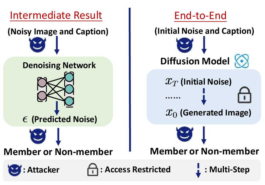
Most existing studies [6]–[10] assumed the adversary can manipulate the intermediate denoising network (denoted as intermediate result attacks). However, this assumption is unrealistic in real-world diffusion systems, which typically expose only end-to-end generation interfaces. Previous end-to-end attacks [5], [11] assumed the availability of auxiliary data drawn from the same distribution as the fine-tuning data, which is used to train shadow models and classifiers. However, such attacks depend heavily on the quality of the auxiliary data, and training shadow models and classifiers incurs substantial computational overhead.
We identify a fundamental vulnerability that enables end-to-end attacks without training shadow models or classifiers: standard noise schedules fail to fully eliminate semantic information from images. Analyzing the widely used schedules, we find the signal-to-noise ratio (SNR) at the maximum noise timestep \(T\) remains non-zero (Tab. 2), leaving residual semantic signals (Observation 1). More critically, via DDIM inversion [12], we find that diffusion models inadvertently learn to exploit these residual signals during training, establishing hidden correlations between initial noise and training data, as evidenced by reconstruction fidelity (Tab. 3) and cross-attention analysis (Fig. 4) (Observation 2).
This presents an exploitable attack opportunity: if we can inject an image’s semantic information into the initial noise, the model’s generation behavior may reveal whether the image belongs to the training set. The key challenge is that adversaries cannot access the target model’s denoising network to perform inversion. Fortunately, we observe that fine-tuned models preserve the semantic space of their pre-trained counterparts (Fig. 4 and Tab. 4), enabling us to use publicly available pre-trained models for semantic injection via DDIM inversion (Observation 3).
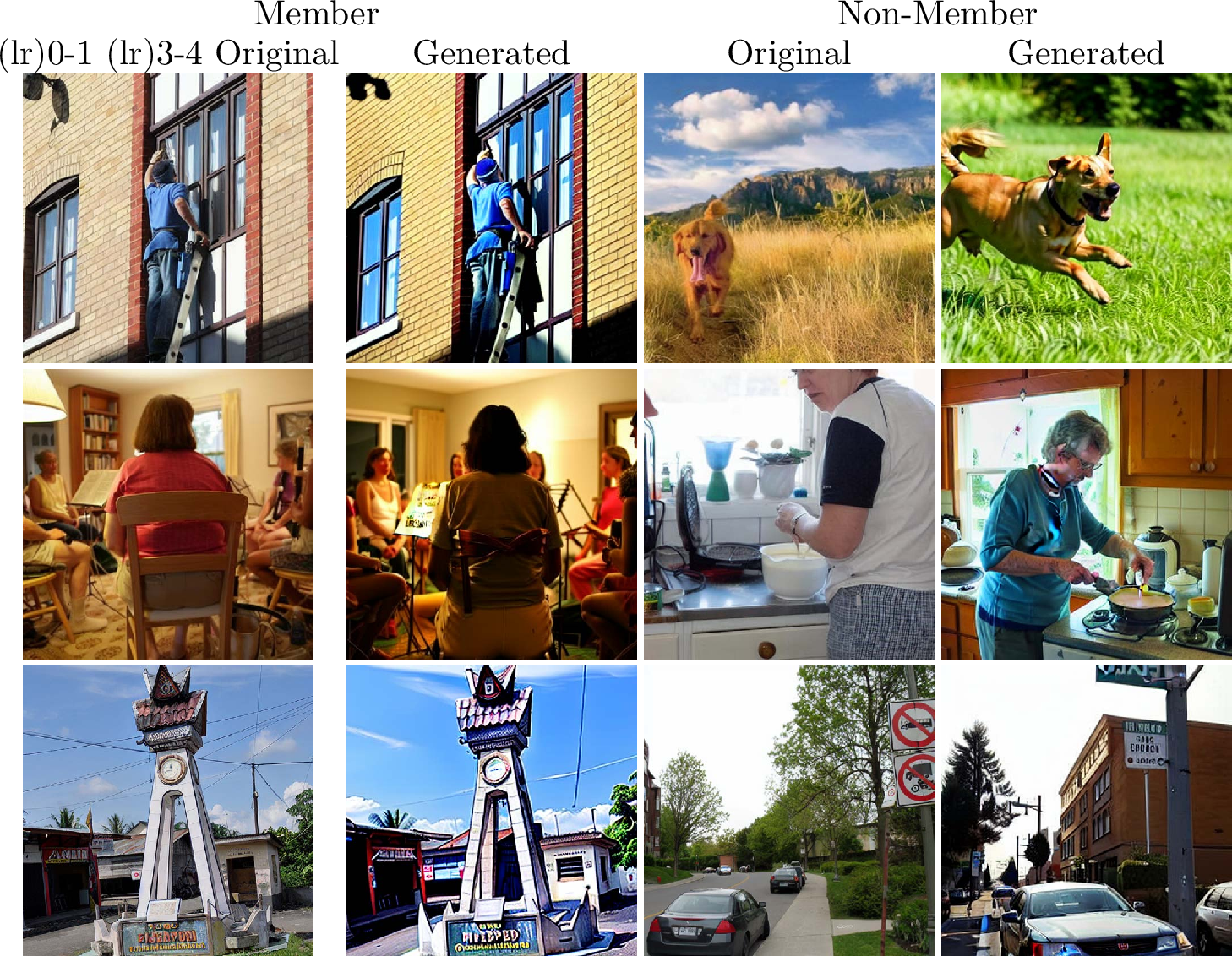
Building on these insights, we propose leveraging a pre-trained model to inject semantic information into the initial noise through a DDIM inversion procedure and determine membership by examining the model’s generation from semantic initial noise. When the model generates images from this semantic noise, members produce outputs significantly closer to their originals than non-members (Fig. 1). This method is an end-to-end attack that requires no access to the target model’s parameters or intermediate denoising network. We compare the conditions of our method with those of previous intermediate result attacks, as illustrated in Fig. 2. Furthermore, our method does not need to train shadow models or classifiers. We summarize our contributions as follows:
To the best of our knowledge, this is the first study to explore the role of initial noise in MIAs against diffusion models. Our key observations indicate that the diffusion model captures hidden correlations between the initial noise and the training data, which serves as a crucial indicator for revealing membership information.
Building on this insight, we propose a simple yet effective membership inference attack that uses the inversion procedure to obtain semantic initial noise. The attack analyzes the model’s generation from initial noise containing the original image semantics, with membership determined by similarity to the original image.
Extensive experiments validate the effectiveness of our method, with an Area Under the Curve (AUC) of 90.46% and a True Positive Rate at 1% False Positive Rate (T@F=1%) of 21.80%. It demonstrates that the initial noise can strongly expose membership information, revealing the vulnerability of diffusion models to MIAs.
2 Related Work↩︎
Membership Inference Attacks. Shokri et al. [3] proposed membership inference attacks (MIAs), which primarily targeted classification models in machine learning. The attacks aim to determine whether a specific piece of data has been included in the training set of the target model. MIAs are typically categorized based on the adversary’s access level to the target model. In the white-box setting, the attacker is assumed to have full access to the model parameters [13]–[16]. In contrast, black-box attacks assume no access to model parameters. Among them, some methods utilize confidence scores or logits provided by the model [3], [17], [18]. Other researchers have proposed attacks under a more restrictive assumption where only the final predicted labels are available [19]–[21].
Membership Inference Attacks on Diffusion Models. Recently, MIAs on diffusion models have garnered increasing attention. Pang et al. [22] proposed executing an attack by utilizing gradient information. Recent works [6]–[10], [23] assumed that the adversary has access to the model’s intermediate denoising process and is allowed to modify the inputs of the denoising networks. This assumption enables queries on the denoising networks’ prediction to infer membership information. Some works [5], [11] relied on an auxiliary dataset drawn from the same distribution to train shadow models, and trained a classifier based on the behavioral differences of the shadow models for member and non-member samples.
Denoising Diffusion Implicit Model (DDIM) Inversion. DDIM Inversion is a technique that utilizes the reverse process of the diffusion model to obtain the initial state of the generated image [12]. In addition, it can be viewed as a noise addition process that integrates semantic information [24], [25]. In contrast, naively adding random noise to the image is not connected to the model’s understanding of the original image’s semantics [26]. Due to the unique advantages of DDIM inversion, it shows great potential in applications such as image quality optimization [24], [25] and image editing [26]–[28].
3 Threat Model↩︎
MIAs aim to determine whether a specific sample was used during the model training. Formally, let \(G_\theta\) be a fine-tuned diffusion model with parameters \(\theta\). Let \(D\) be a dataset drawn from the data distribution \(q_{\mathrm{data}}\) and each sample \(x_i\) in \(D\) has a caption \(\mathbf{c}_i\). Following established conventions [7], [15], [18], we split \(D\) into two subsets \(D_M\) and \(D_N\), where \(D_M\) denotes the member set used to fine-tune the diffusion model \(G_\theta\) and \(D_N\) denotes the non-member set, so that \(D = D_M \cup D_N\) and \(D_M \cap D_N = \varnothing\). Each image sample \(x_i\) is associated with a membership label \(m_i\), where \(m_i=1\) if \(x_i\in D_M\) and \(m_i=0\) otherwise. The adversary has access to the dataset \(D\), but does not know the partition.
Adversary’s Goal. The adversary’s goal is to design a membership inference attack algorithm \(\mathcal{A}\) that, for any sample \(x_i\), predicts its membership label: \[\mathcal{A}(x_i, \theta) = \mathbb{1} \left[ \mathbb{P}(m_i = 1 \mid \theta, x_i) \geq \tau \right],\] where \(\mathcal{A}(x_i, \theta) = 1\) means \(x_i\) comes from \(D_M\), \(\mathbb{1} [A] = 1\) if \(A\) is true, and \(\tau\) is the threshold.
Adversary’s Capabilities. In this paper, the adversary is limited to performing end-to-end generation using the diffusion model. Specifically, the adversary can modify the model’s initial noise and prompt, and can only observe the final generated image, but has no access to any model parameters or intermediate denoising steps. In the diffusers library [29], pipeline interfaces can accept an initial noise input, which can be adjusted to guide the generation process. Moreover, tasks such as image editing [25], [30], [31], and noise engineering [27], [32], [33] also rely on interfaces that allow the modification of the initial noise. The fine-tuned model is obtained by fine-tuning a pre-trained model on a downstream dataset. Following prior membership inference settings for fine-tuned models [5], [7], [10], [34], we assume that the adversary has access to the pre-trained version of the fine-tuned model.1 We compare the capabilities of adversaries across different attack algorithms in Tab. 1.
| Method | Pm | Inter | Shadow | Arch | cls |
|---|---|---|---|---|---|
| GSA [22] | |||||
| Loss [6] | |||||
| SecMI [7] | |||||
| PIA [8] | |||||
| CLiD [10] | |||||
| NA-P [11] | |||||
| Feature-T [5] | |||||
| Feature-C [5] | |||||
| Feature-D [5] | |||||
| Ours |
4 Methodology↩︎
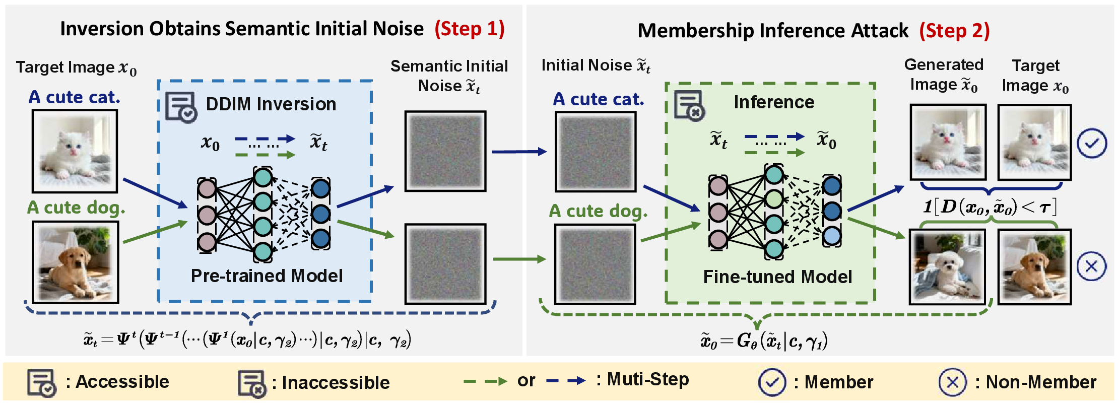
In this section, we present our three key observations systematically. Based on these observations, we propose a membership inference attack that leverages initial noise, which is performed in two steps, as shown in Fig. 3.
4.1 Diffusion Models↩︎
Given an original image \(x_0\), the forward diffusion process gradually introduces noise over \(T\) timesteps, transforming \(x_0\) into a nearly Gaussian-distributed \(x_T\). The forward diffusion process at each timestep \(t\) is described as follows: \[x_t = \sqrt{\bar{\alpha}_t} x_0 + \sqrt{1 - \bar{\alpha}_t} \epsilon,\] where \(\overline{\alpha}_t = \prod_{i=1}^{t} \alpha_i\) and \((\alpha_1, \ldots, \alpha_T)\) are the noise schedules, \(\epsilon \sim \mathcal{N}(0, I)\) represents Gaussian noise at each step. As \(t\) approaches \(T\), \(\bar{\alpha}_t\) diminishes, making \(x_T \approx \epsilon\) closely resemble pure Gaussian noise. In this paper, we use \(\epsilon_\theta\) to denote the prediction of the denoising network.
4.2 The Semantics in Initial Noise↩︎
Observation 1. The widely adopted noise schedules fail to eliminate the semantic information in the original image, even at the maximum noise step.
Explanation 1. We begin with the forward noise addition process in diffusion models. We follow the definition of the signal-to-noise ratio (SNR) in the diffusion model training process from prior work [35]. For a given timestep \(t\), SNR can be characterized as follows: \[\text{SNR}(t) := \bar{\alpha}_t/(1 - \bar{\alpha}_t).\] We compared the SNR of images at step \(T\) across different schedules in Tab. 2. Consistent with the analyses in prior work [30], [36], noise injection at step \(T\) cannot eliminate the original signal.
| Schedule | \(\text{SNR}(T)\) | \(\sqrt{\bar{\alpha}_T}\) |
|---|---|---|
| Linear | 4.04e-05 | 0.006353 |
| Cosine | 4.24e-09 | 0.00004928 |
| Stable Diffusion | 4.68e-03 | 0.068265 |
The diffusion model’s training process can be interpreted as learning a transformation from a Gaussian noise distribution to a Gaussian image distribution. Previous studies on noise engineering [24], [25], [30], [31] have shown that the initial noise contains semantic information that influences the generation process. Based on the evidence above, we speculate that the semantics of the initial noise may be linked to the training data, potentially revealing membership information. Our subsequent observation further supports this speculation.
Observation 2. The diffusion model inadvertently learns to exploit residual information in the initial noise, thereby establishing a hidden connection between the initial noise and the training data.
Explanation 2(a). As discussed in Sec. 2, DDIM inversion can be regarded as a noise injection process that embeds the semantics of the original image into the initial noise. The inversion process \(\Psi\) can be expressed as follows: \[\begin{align} \label{inversion} \tilde{x}_t = \Psi^t(\tilde{x}_{t-1} | \mathbf{c}, \gamma_2) &= \sqrt{\overline{\alpha}_{t}} \tilde{f}_\theta(\tilde{x}_{t-1}, t-1) \\ &+ \sqrt{1 - \overline{\alpha}_{t}}\epsilon_\theta(\tilde{x}_{t-1}, t-1), \end{align}\tag{1}\] where \(\tilde{f}_\theta(\tilde{x}_{t-1}, t-1)\) can be expressed as: \[\tilde{f}_\theta(\tilde{x}_{t-1}, t-1) = \frac{\tilde{x}_{t-1}-\sqrt{1 - \overline{\alpha}_{t-1}} \epsilon_\theta(\tilde{x}_{t-1}, t-1)}{\sqrt{\overline{\alpha}_{t-1}}},\] where \(\epsilon_\theta(\tilde{x}_{t-1}, t-1) = (1+\gamma_2) \epsilon_\theta(\tilde{x}_{t-1}, \mathbf{c}, t-1) - \gamma_2 \epsilon_\theta(\tilde{x}_{t-1}, \varnothing, t-1)\), \(\mathbf{c}\) is the text prompt, \(\varnothing\) represents the null prompt and \(\gamma_2\) is the inversion guidance scale. Analyzing the diffusion model’s training process and the characteristics of DDIM inversion, we attempt to use the target model for DDIM inversion to obtain semantic initial noise, which can be expressed as: \[\small \begin{align} \tilde{x}_t & = Inv^t_{\theta}(x_0|\mathbf{c}, \gamma_2) \\ &= \Psi^t\Big( \Psi^{t-1}\big( \cdots (\Psi^1(x_0 \mid \mathbf{c}, \gamma_2)\cdots)\mid \mathbf{c},\gamma_2\big)\mid \mathbf{c},\gamma_2 \Big). \end{align}\] Then, we use the obtained noise as the starting point for image generation, which can be formulated as: \[\tilde{x}_0=G_\theta(\tilde{x}_t|\mathbf{c}, \gamma_1).\] where \(\gamma_1\) is the guidance scale during generation. We compared the normalized \(\ell_{2}\) distance between the original images and those generated from random noise or semantic noise (obtained via inversion). Tab. 3 reports the statistical results for both member and non-member samples across different datasets. The results demonstrate that semantic initial noise leads to higher fidelity reconstructions of the training data. This confirms that diffusion models capture residual information from images, and when conditioned on initial noise containing member semantics, they generate outputs that are closer to the original member images.
| Pokémon | MS-COCO | Flickr | |||||
|---|---|---|---|---|---|---|---|
| 2-3 (lr)4-5 (lr)6-7 | Mem | Non-Mem | Mem | Non-Mem | Mem | Non-Mem | |
| \(Random\) | 0.3839 | 0.3961 | 0.4034 | 0.4963 | 0.3543 | 0.3972 | |
| \(Inversion\) | 0.2779 | 0.5061 | 0.2469 | 0.5394 | 0.2722 | 0.4464 | |
| \(\Delta\) | -0.1060 | +0.1100 | -0.1565 | +0.0431 | -0.0821 | +0.0492 | |
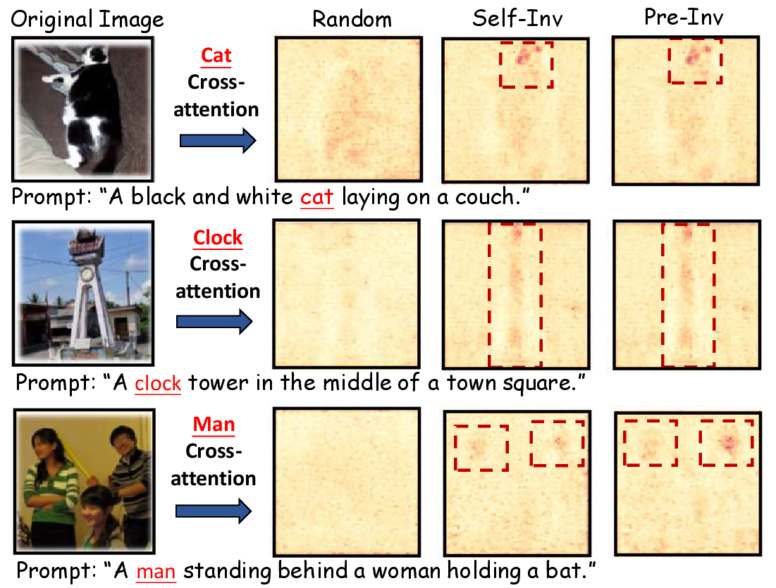
Explanation 2(b). Previously, we observed that DDIM inversion enables better reconstruction of member data. We attribute this to the model having learned correlations between residual semantics and the original images during training. To further validate this hypothesis, we analyze the cross-attention of the denoising network during the generation process. Specifically, we visualize the cross-attention heatmaps at the first denoising step, which compute the attention of the token corresponding to the main object in the image. As shown in Fig. 4, when using initial noise obtained via DDIM inversion, the denoising network immediately attends to the semantic regions of the image. In contrast, when initialized with random noise, the network exhibits no clear focus on specific regions. This phenomenon further proves that the model has established a hidden connection between the initial noise and the original image.
4.3 Semantic Injection via the Pre-trained Model↩︎
One major challenge is that the adversary cannot directly access the parameters of the target model, making it infeasible to perform DDIM inversion on the target itself. Despite these constraints, we observe a crucial aspect of fine-tuning in the context of membership inference attacks.
Observation 3. Models fine-tuned from pre-trained ones essentially preserve the original semantic space and representational capabilities.
Explanation 3. Previous works [40], [41] suggested that fine-tuning does not substantially alter the original distribution. Based on this characteristic, we hypothesize that the model’s understanding and representation of semantic information have not undergone significant changes after fine-tuning. To verify this hypothesis, we perform inversion with the pre-trained version of the target model to obtain semantic initial noise. Following the same procedure as before, we then feed this noise into the target model and examine its cross-attention heatmaps. As shown in Fig. 4, the fine-tuned model still captures the semantics in the initial noise, with high cross-attention similarity to that obtained from self-inversion2.
To further confirm this similarity, we computed the cosine similarity of cross-attention heatmaps between the initial noise obtained from self-inversion and pre-inversion. As shown in Tab. 4, across different fine-tuning epochs, the cross-attention heatmaps of the noise from the two inversions exhibit a remarkably high degree of similarity. Additionally, we have provided an analysis of model parameter similarity in Appendix 9.4. All the findings provide evidence that the fine-tuned model retains the semantic space of its pre-trained version, making it possible to obtain semantic initial noise using a pre-trained model.
| Epoch | 50 | 100 | 150 | 200 | 250 | 300 |
|---|---|---|---|---|---|---|
| Pokémon | 0.968 | 0.942 | 0.926 | 0.897 | 0.895 | 0.892 |
| T-to-I | 0.970 | 0.954 | 0.924 | 0.899 | 0.893 | 0.893 |
| MS-COCO | 0.973 | 0.953 | 0.937 | 0.897 | 0.895 | 0.895 |
| Flickr | 0.978 | 0.953 | 0.934 | 0.904 | 0.902 | 0.903 |
| Pokémon | T-to-I | MS-COCO | Flickr | Average | |||||||
|---|---|---|---|---|---|---|---|---|---|---|---|
| 2-3 (lr)4-5 (lr)6-7 (lr)8-9 (lr)10-11 | AUC | T@F=1% | AUC | T@F=1% | AUC | T@F=1% | AUC | T@F=1% | AUC | T@F=1% | |
| SecMI | 83.26 | 12.88 | 88.26 | 26.66 | 89.37 | 16.79 | 76.42 | 14.40 | 84.33 | 17.68 | |
| PIA | 76.82 | 7.85 | 84.80 | 11.78 | 71.38 | 5.20 | 72.59 | 7.20 | 76.40 | 8.01 | |
| NA-P | 59.37 | 4.80 | 70.77 | 6.60 | 52.41 | 2.20 | 56.51 | 4.00 | 59.77 | 4.40 | |
| GD | 52.67 | 1.20 | 59.67 | 5.20 | 51.22 | 1.00 | 53.41 | 2.00 | 54.24 | 2.35 | |
| Feature-T | 56.60 | 3.00 | 70.40 | 7.00 | 57.70 | 3.20 | 58.20 | 3.00 | 60.73 | 4.05 | |
| Feature-C | 60.67 | 7.33 | 83.77 | 17.40 | 73.08 | 14.60 | 63.80 | 5.20 | 70.33 | 11.13 | |
| Feature-D | 55.10 | 2.80 | 65.00 | 6.00 | 58.00 | 3.00 | 57.20 | 3.00 | 58.83 | 3.70 | |
| Ours | 82.44 | 14.00 | 89.24 | 21.60 | 90.46 | 21.80 | 76.23 | 16.00 | 84.59 | 18.35 | |
4.4 MIAs Leveraging Initial Noise↩︎
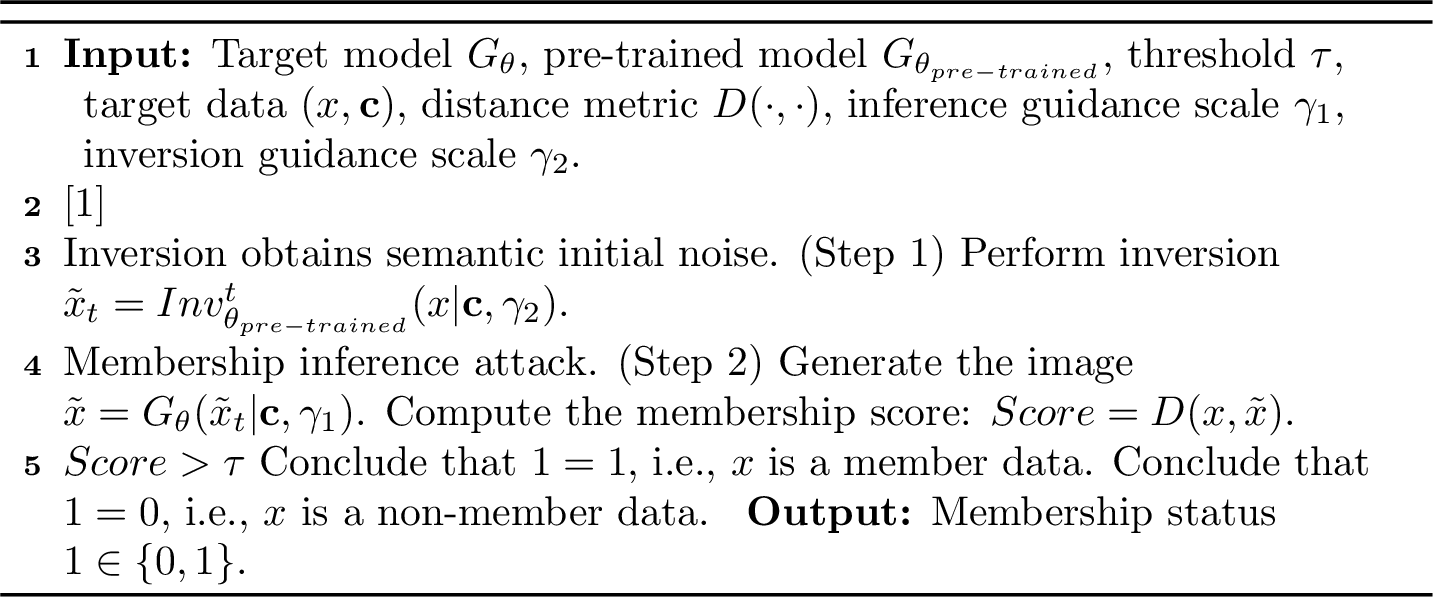
Based on the above experiments and observations, we propose a simple yet effective membership inference attack that exploits the correlations between the semantic initial noise and the training data. This attack proceeds in two main steps: obtaining semantic initial noise and conducting the membership inference attack. We provide the detailed algorithmic procedure in Appendix 8.
Step 1: Given a target image \(x_0\) and its corresponding text prompt \(\mathbf{c}\), we first employ a pre-trained diffusion model to perform DDIM inversion, thereby obtaining a semantic initial noise \(\tilde{x}_t\).
Step 2: The adversary feeds the semantic initial noise \(\tilde{x}_t\) and the same prompt \(\mathbf{c}\) into the target model to generate a candidate image \(\tilde{x}_0\). If the target image \(x_0\) was part of the fine-tuning dataset, the generated candidate image tends to preserve its structural and semantic consistency, resulting in a smaller perceptual distance. Conversely, the non-member samples will yield larger deviations in the generated outputs. The membership inference decision is made by comparing the reconstruction distance using a metric \(D(\cdot, \cdot)\). In summary, our method can be summarized as follows: \[\small \begin{cases} \tilde{x}_{t} = Inv^t_{\theta_{pre-trained}}(x_0|\mathbf{c}, \gamma_2), \;\textcolor{red}{(Step\;1)}\\[4pt] \mathcal{A}(x_i, \theta) = \mathbb{1} \left[ D(x_0, G_\theta(\tilde{x}_{t}|\mathbf{c},\gamma_1)) \leq \tau \right]. \; \textcolor{red}{(Step\;2)} \end{cases}\] where \(D(\cdot, \cdot)\) represents the distance metric.
5 Experiments↩︎
5.1 Experiment Setup↩︎
Datasets and Models. We follow the previous stringent assumption that both member and non-member data are drawn from the same distribution [7], [8], [10], [23]. We construct member/non-member datasets using 416/417 samples from Pokémon [42], 500/500 samples from text-to-image-2M (T-to-I) [43], 2500/2500 samples from MS-COCO [44], and 1000/1000 samples from Flickr [45]. We fine-tune Stable Diffusion-v1-4 (SD-v1-4) [46] using the official fine-tuning scripts from the Hugging-Face Diffusers library [47]. The detailed fine-tuning configurations are provided in Appendix 9.1.
Evaluation Metrics. We adopt the evaluation metrics commonly used in prior membership inference attacks for large models [5], [7], [8], [34], [48]. Specifically, we report the Area Under the Curve (denoted as AUC), which reflects the average success of membership inference attacks. In addition, we measure the True Positive Rate (TPR) at 1% False Positive Rate (FPR) (denoted as T@F=1%), which assesses attack efficacy under a strict decision threshold, emphasizing performance at an extremely low FPR.
Baselines. We compare our method with existing end-to-end attacks, including NA-P [11], Feature-T [5], Feature-D [5], Feature-C [5], and GD [49]. We also evaluate intermediate result attacks, including SecMI [7] and PIA [8].
Implementation Details. All fine-tuning and inference experiments were conducted on a single RTX 4090 GPU (24 GB). During the DDIM inversion step, we set the guidance scale \(\gamma_2 = 1.0\) and the number of steps \(i_{\text{step}} = 100\). For the membership inference step, we set the guidance scale \(\gamma_1 = 3.5\) and the number of inference steps to \(50\). We use the \(\ell_{2}\) distance as the \(D(\cdot, \cdot)\) by default.
| \(\gamma_{2}=0.0\) | \(\gamma_{2}=1.0\) | \(\gamma_{2}=3.5\) | \(\gamma_{2}=4.5\) | \(\gamma_{2}=7.5\) | |||||||
|---|---|---|---|---|---|---|---|---|---|---|---|
| 2-3 (lr)4-5 (lr)6-7 (lr)8-9 (lr)10-11 | AUC | T@F=1% | AUC | T@F=1% | AUC | T@F=1% | AUC | T@F=1% | AUC | T@F=1% | |
| \(i_{step}=25\) | 89.20 | 21.40 | 89.16 | 21.40 | 87.36 | 21.00 | 87.46 | 21.20 | 87.25 | 21.00 | |
| \(i_{step}=50\) | 87.36 | 21.20 | 87.24 | 21.00 | 89.14 | 21.20 | 89.36 | 21.60 | 89.33 | 21.40 | |
| \(i_{step}=100\) | 88.48 | 21.00 | 90.46 | 21.80 | 88.56 | 21.00 | 88.61 | 21.00 | 90.12 | 21.80 | |
| \(i_{step}=200\) | 89.12 | 21.20 | 89.12 | 21.40 | 91.00 | 22.00 | 91.04 | 22.00 | 89.31 | 21.20 | |
5.2 Main Result↩︎
Overall Attack Performance. We report comprehensive attack results and compare the performance of our method against all baselines. As shown in Tab. 5, our method consistently achieves superior performance across different datasets, delivering significant improvements over existing end-to-end attacks. In particular, compared to the state-of-the-art (SOTA) end-to-end attack, Feature-C, our method can yield improvements of up to 21.77% in AUC and 11.80% in TPR@1%FPR. Notably, Feature-C requires auxiliary data to train shadow models and classifiers, resulting in significant training overhead. In contrast, our method performs the attack solely through threshold setting, achieving superior performance with a lower computational cost. Moreover, our method remains highly competitive compared to intermediate result attacks, e.g., SecMI and PIA, and outperforms them on the MS-COCO dataset, all while not requiring access to the intermediate results.
| Pokémon | T-to-I | MS-COCO | Flickr | ||||||
|---|---|---|---|---|---|---|---|---|---|
| 2-3 (lr)4-5 (lr)6-7 (lr)8-9 | AUC | T@F=1% | AUC | T@F=1% | AUC | T@F=1% | AUC | T@F=1% | |
| Naive | 55.66 | 6.50 | 72.76 | 10.50 | 62.24 | 7.00 | 57.29 | 5.00 | |
| Ours | 82.44 | 14.00 | 89.24 | 21.60 | 90.46 | 21.80 | 76.23 | 16.00 | |
| Gain | +26.78 | +7.50 | +16.48 | +11.10 | +28.22 | +14.80 | +18.94 | +11.00 | |
Visual Analysis of Attack Performance. To further illustrate the effectiveness of our method, we compare it against Feature-T, the previous most potent threshold-based end-to-end attack. As shown in Fig. 5, we visualize the membership score distributions of member and non-member data. The separation between the two distributions achieved by our method is substantially larger than that of Feature-T. This visualization provides intuitive evidence of the enhanced distinguishability achieved by our method.
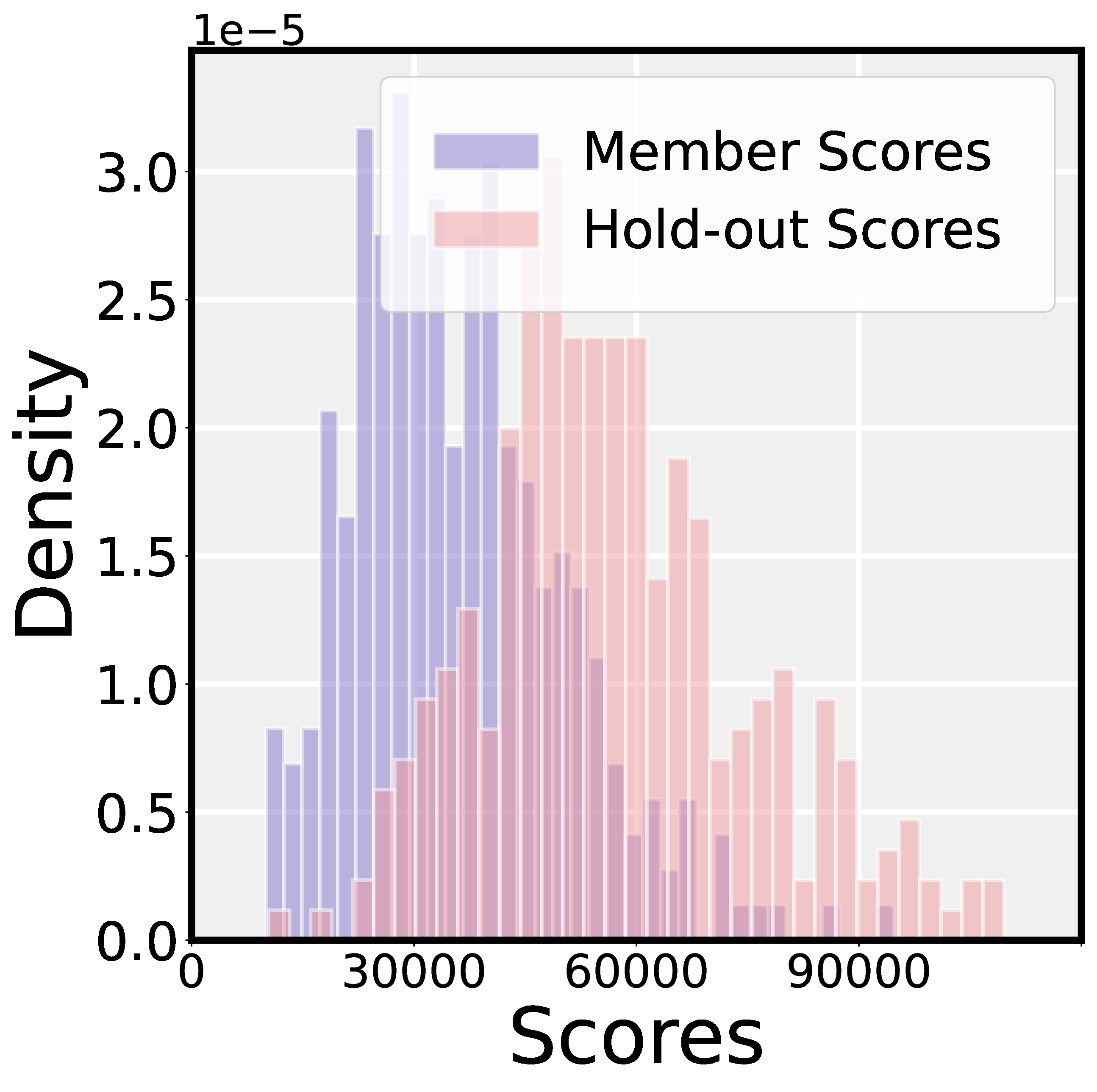


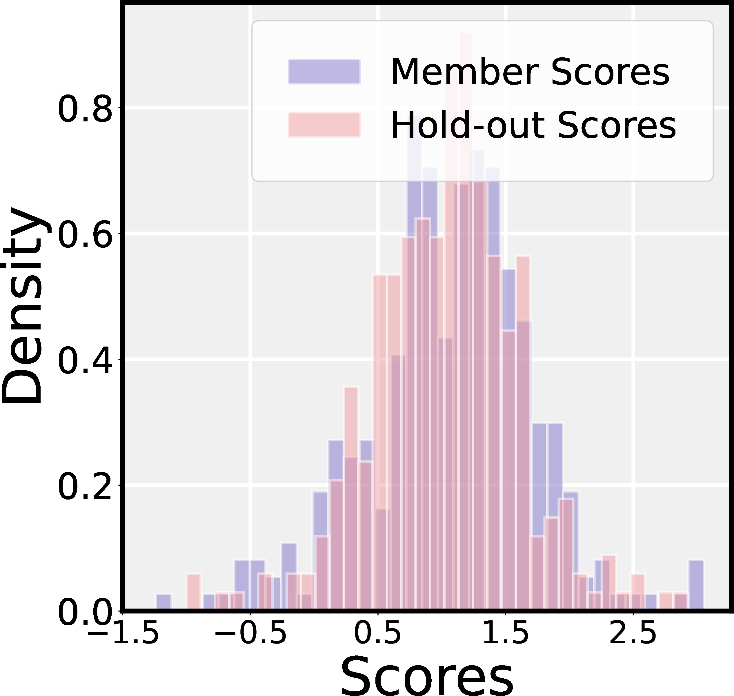
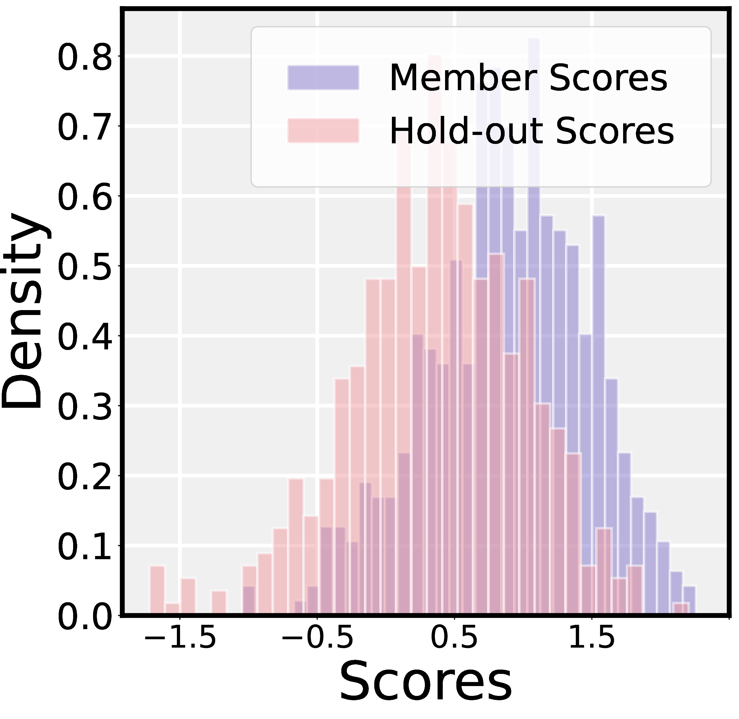

Figure 5: Membership score distribution of member and non-member data in the Pokémon, T-to-I, and MS-COCO dataset, arranged from left to right. The score distribution gap between member data and hold-out data is significantly larger in our method..
5.3 Ablation Study↩︎
Contribution of Semantic Initial Noise. In this section, we define the Naive method, which generates images solely from the given caption using randomly initialized noise. The distance between the generated image and the target image is
then measured to determine membership. The ablation results are reported in Tab. 7. On average, the AUC improved by 21.57% across different datasets, and T@F=1% increased by 10.63%. It clearly shows that injecting semantics into
the initial noise substantially improves the attack performance. These results validate the effectiveness of our approach and underscore the importance of carefully managing and protecting initial noise.
Ablation on Hyperparameter. We validate the impact of hyperparameters \(i_{step}\) and \(\gamma_{2}\) on the performance of our method. As shown in Tab. 6, our method demonstrates very low sensitivity to \(i_{step}\) and \(\gamma_{2}\), with the best and worst AUC being 91.04% and 87.25%, respectively (a
variation of only 3.79%). It provides strong confirmation of the robustness of our method. Further analyses on hyperparameters are presented in Appendix 9.9.
| \(SS_{e_i}\) | DataAug | SecMI | PIA | NA-P | GD | Feature-T | Feature-C | Feature-D | Ours | |
|---|---|---|---|---|---|---|---|---|---|---|
| \(\times\) | \(\times\) | 89.43 | 74.36 | 64.77 | 51.31 | 59.43 | 73.26 | 59.01 | 91.12 | |
| \(\times\) | \(✔\) | 89.37 | 71.38 | 63.41 | 51.22 | 57.70 | 73.08 | 58.00 | 90.46 | |
| \(✔\) | \(\times\) | 52.11 | 58.93 | 62.98 | 51.05 | 57.53 | 71.99 | 57.20 | 87.68 | |
| \(✔\) | \(✔\) | 51.21 | 54.41 | 62.56 | 51.03 | 57.20 | 71.02 | 57.50 | 86.74 |
5.4 A More Knowledge-Restricted Adversary↩︎
Without Access to the Model Architecture. In real-world scenarios, model publishers may deliberately withhold the architecture version of the pre-trained model used during fine-tuning, thereby increasing the difficulty of attacks. To evaluate performance under this condition, we use SD-v1-5 [50], SD-2-1 [51], SDXL-turbo [52], and Dreamshaper-XL [53] to perform inversion and obtain initial noise, where the architectural discrepancy from the SD-v1-4 gradually increases. And these models are used as shadow models for the baseline attacks. As shown in Tab. 9, our method remains effective even when the architecture version of the target model is unknown. Although all methods exhibit performance degradation as the architectural gap widens, our method achieves the best performance even using SDXL-turbo and Dreamshaper-XL, whose architectures differ substantially from the target model. This finding aligns with the observations in [30], which indicate that the semantics of the initial noise can be transferred across models due to the shared distributions learned during large-scale pre-training. This further validates that semantic initial noise can be leveraged to reveal membership information.
| SD-v1-5 | SD-2-1 | SDXL-turbo | Dreamshaper | ||||||
|---|---|---|---|---|---|---|---|---|---|
| 2-3 (lr)4-5 (lr)6-7 (lr)8-9 | AUC | T@F=1% | AUC | T@F=1% | AUC | T@F=1% | AUC | T@F=1% | |
| NA-P | 70.53 | 6.60 | 69.21 | 6.60 | 55.53 | 2.20 | 56.02 | 2.40 | |
| Feature-C | 83.41 | 17.40 | 81.28 | 16.70 | 68.41 | 6.20 | 67.42 | 6.00 | |
| Feature-D | 65.00 | 6.00 | 64.59 | 6.00 | 58.00 | 4.00 | 57.66 | 4.20 | |
| Ours | 89.03 | 20.20 | 88.04 | 19.60 | 76.91 | 8.40 | 76.87 | 8.20 | |
Lacking Access to Image Captions. In reality, attackers may not have the image captions used for fine-tuning. Therefore, we also evaluate the attack performance when the image captions are unavailable. To address this, we employ BLIP [54] to generate captions for the images and use these generated captions to conduct the attack. Experimental results show that our method remains effective even without access to the original captions. The detailed experimental results are provided in Appendix 9.6.
5.5 Impact of Defense↩︎
To assess the robustness of our method, we investigate the impact of the SOTA defense method \(SS_{e_i}\) [1]. This defense dynamically evaluates the model’s memorization during training and adjusts the training process accordingly. Following this method, we set the \(SS_{e_i}\) threshold to \(4\). Additionally, data augmentation techniques are commonly employed to mitigate MIAs. During the fine-tuning process of the diffusion model, Random-Crop and Random-Flip are applied by default [47]. Following previous work [7], [10], [22], we also investigate the impact of data augmentation on the performance of attacks. We conduct an in-depth analysis of the performance changes of various attacks before and after applying defenses on the MS-COCO dataset, as shown in Tab. 8. Experimental results show that our method maintains excellent performance even against the advanced defense strategies. In the presence of both defense mechanisms, our method achieves substantially better performance than all the other methods. Specifically, the intermediate result attacks show a significant performance drop under defense. In our method, AUC and TPR@1%FPR decrease by only 4.38% and 5.00%, respectively, compared to performance without any defense. These results underscore the strong robustness of our method. We provide the results of T@F=1% in the Appendix 9.11.
5.6 Visualization of Generated Results.↩︎
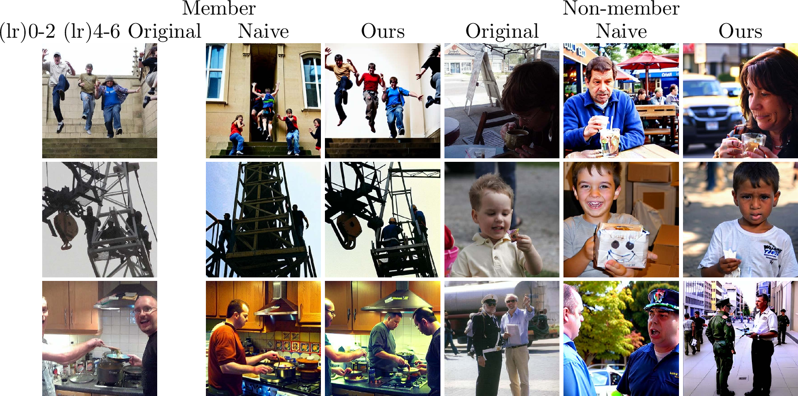
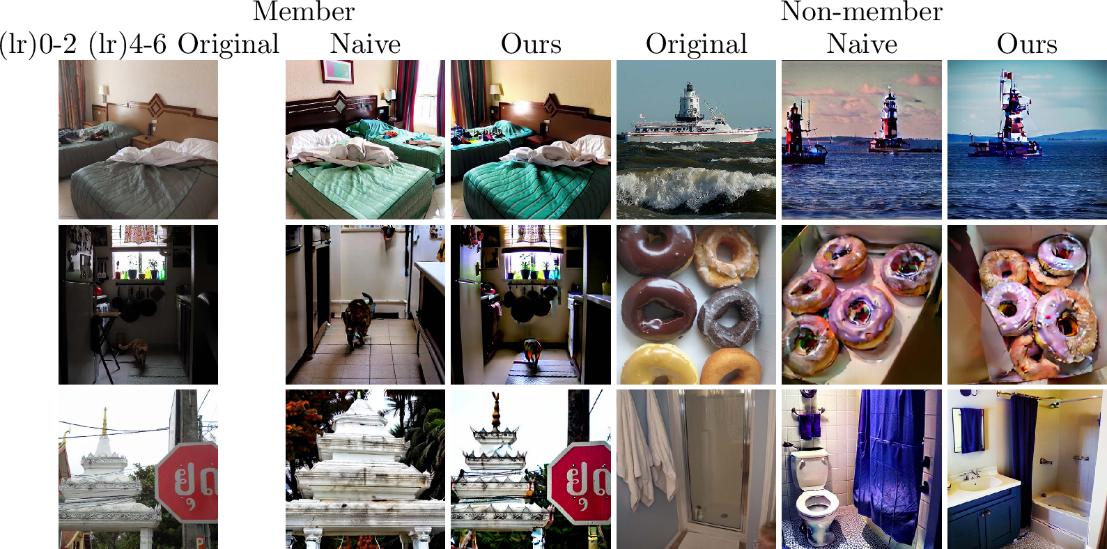
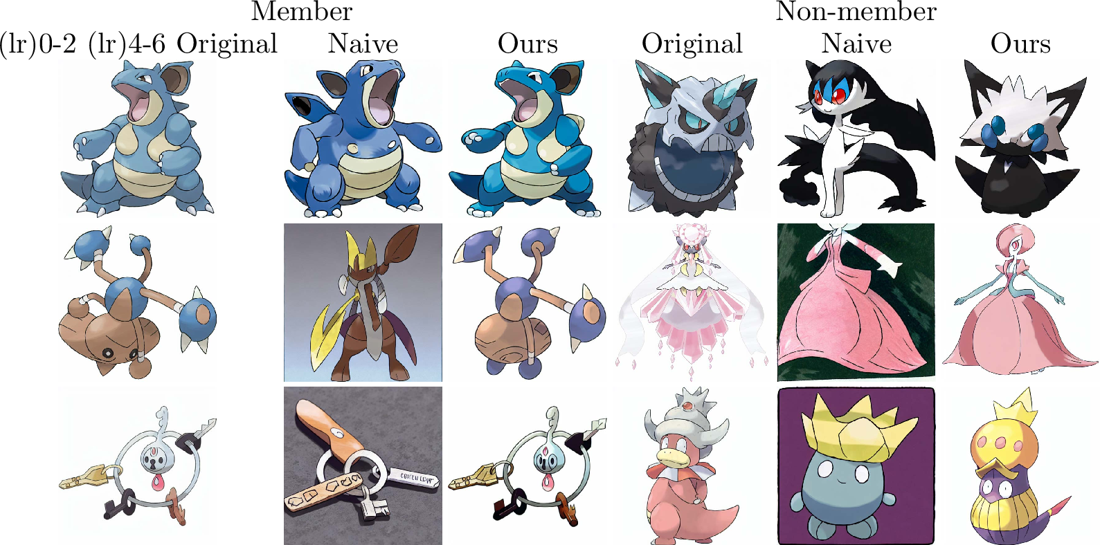
We present the generation results for member and non-member samples in Fig. 6. The first three columns display the original member images alongside their generated counterparts, using both random and semantic initial noise. The last three columns show non-member images and their corresponding generated results. In Naive, the generated results, whether from member or non-member samples, significantly deviate from the originals. Our method generates member images that closely resemble their originals, and the generated non-member images differ more noticeably. This discrepancy is the primary reason for our high attack performance. More visualizations are provided in Appendix 9.5.
6 Conclusion↩︎
In this paper, we reveal that standard noise schedules in diffusion models retain residual semantic information in the initial noise, which the model inadvertently exploits to learn training data correlations. Leveraging this vulnerability, we propose a simple yet effective membership inference attack that uses DDIM inversion to inject semantics into the initial noise and analyzes the resulting generations. Our experiments confirm that these semantic residuals pose significant privacy risks in fine-tuned models.
7 More Details for Related Work↩︎
Classifier-free Guidance. Controllable generation can be achieved by adjusting the semantic representation during denoising. In classifier-free guidance training [55], the denoising network \(\epsilon_\theta\) is jointly trained under both conditional and unconditional settings. At inference time, for a sample \(x_t\) at timestep \(t\), the denoising result is obtained by interpolating between the conditional and unconditional predictions of \(\epsilon_\theta\), which
allows the guidance scale \(\gamma\) to be flexibly tuned: \[\epsilon_\theta(x_t, t) = (1+\gamma)\,\epsilon_\theta(x_t, \mathbf{c}, t) - \gamma\,\epsilon_\theta(x_t, \varnothing, t),\]
where \(\varnothing\) represents the null prompt, corresponding to the unconditional denoising result.
Denoising Diffusion Implicit Model (DDIM). DDIM [37] enables the diffusion model to skip timesteps, thereby greatly accelerating the sampling
process. The denoising process \(\Phi^{t}(x_t \mid \mathbf{c}, \gamma_1)\) can be expressed as: \[\begin{align}
x_{t-1} = & \; \Phi^{t}(x_t \mid \mathbf{c}, \gamma_1) \\ =
& \sqrt{\overline{\alpha}_{t-1}} f_{\theta}(x_t, t) + \sqrt{1 - \overline{\alpha}_{t-1}}\epsilon_\theta(x_t, t),
\end{align}\] where \(f_{\theta}(x_t, t)\) can be expressed as: \[f_{\theta}(x_t, t)=\frac{x_t-\sqrt{1 - \overline{\alpha}_t} \epsilon_\theta(x_t, t)}{\sqrt{\overline{\alpha}_t}},\]
where \(\epsilon_\theta(x_t, t) = (1+\gamma_1) \epsilon_\theta(x_t, \mathbf{c}, t) - \gamma_1 \epsilon_\theta(x_t, \varnothing, t)\).
Cross-Attention Layer. In diffusion models, text-image correspondence is established through the cross-attention mechanism, which enables text-guided generation. A given caption \(\mathbf{y} = \{y_1, y_2, \cdots,
y_n\}\) is first embedded into a sequential representation using the pre-trained CLIP text encoder [56], yielding the
conditioning vector \(\mathbf{c} = f_{\text{CLIP}}(\mathbf{y})\), where \(\mathbf{c}=\{c_1, c_2, \cdots, c_m\}\). Linear projections are applied to extract the key \(\mathbf{K}\) and value \(\mathbf{V}\) from \(\mathbf{c}\), while the query \(\mathbf{Q}\) is derived from the intermediate
features of the denoising network. The cross-attention map \(\mathbf{Attention}^\mathbf{c}\) is then computed as: \[\mathbf{Attention}^\mathbf{c} =
\text{softmax}\!\left(\frac{\mathbf{Q}\mathbf{K}^T}{\sqrt{d}}\right),\] where \(d\) denotes the dimension of the feature space. We use \(\mathbf{Attention}^\mathbf{c}_{y_i}\) as the
attention map, which represents the probability of token \(y_i\) at spatial location in the feature map of the denoising network.
Defense Against Exact Memorization. Wen et al. [1] identified that when a model exactly memorizes training data, the noise
prediction network exhibits a pronounced discrepancy between its conditional and unconditional predictions. Given a training data \(x\), and the caption embedding \(\mathbf{c}\) consisting
of \(N\) tokens, they formulate the minimization objective at step \(t\) as: \[\mathcal{L}(x_t, \mathbf{c}) = \left\| \epsilon_{\theta}(x_t, \mathbf{c}, t) -
\epsilon_{\theta}(x_t, \varnothing, t) \right\|_2.\] The memorization score for each token at position \(i \in [0, N-1]\) is then defined as: \[SS_{\mathbf{c}_{i}} = \frac{1}{T}
\sum_{t=1}^{T} \left\| \nabla_{c_{i}} \mathcal{L}(x_t, \mathbf{c}) \right\|_2.\] To mitigate memorization, they propose excluding a sample from the mini-batch whenever the memorization score exceeds a predefined threshold, thereby skipping the loss
computation for that sample. Since the model has already seen such samples during training, their removal is unlikely to degrade overall model performance. This method has been proven to significantly alleviate exact memorization of training samples,
thereby protecting the privacy of the training set.
8 Detailed Algorithm↩︎
We provide a detailed procedure for our method in Algorithm 7, which can be divided into two main steps.
9 More Details about Experiment↩︎
9.1 More Detailed settings↩︎
As shown in Tab. 10, we report the partition of member and non-member data for all datasets, ensuring that both subsets are independently and identically distributed with equal sizes. In addition, we provide the training configurations, including batch size, number of iterations, and learning rate.
| Dataset | Resolution | Member | Hold-out | Learning rate | Iterations | Batch-size | |
|---|---|---|---|---|---|---|---|
| Pokémon | 512 | 416 | 417 | 1e-04 | 15000 | 1 | |
| T-to-I | 512 | 500 | 500 | 1e-04 | 30000 | 1 | |
| Flickr | 512 | 1000 | 1000 | 1e-04 | 60000 | 1 | |
| MS-COCO | 512 | 2500 | 2500 | 1e-04 | 150000 | 1 |
9.2 Threshold Choosing↩︎
The adversary can determine the threshold for membership inference based on specific performance requirements. For instance, a higher (lower) threshold can be adopted to prioritize precision (recall), depending on the objective of the attack. In this study, we don’t train a shadow models to obtain the threshold due to the expensive computational overhead. Instead, we follow the threshold choosing established in prior work [17]. Specifically, [17] proposed that non-member data is readily accessible, as it can be easily obtained from the internet or generation. The adversary only requires prior access to a subset of non-member samples. Then, adversary queries the membership scores of these non-member samples and selects the \(k\)-th percentile as the threshold.
Following this strategy, we set \(k=15\) to determine the attack threshold across various datasets. We evaluate the effectiveness of the threshold selection using the Attack Success Rate (ASR), which is equivalent to the binary classification accuracy. Tab. 11 presents a comparative analysis between our method and various baselines. The results demonstrate that such a straightforward thresholding approach yields good attack performance. Specifically, our method achieves best performance among end-to-end attacks and remains highly competitive against intermediate result attacks, particularly delivering superior performance on the T-to-I and MS-COCO datasets.
| Dataset | Pokemon | T-to-I | MS-COCO | Flickr | Average |
|---|---|---|---|---|---|
| SecMI | 76.21 | 81.10 | 81.70 | 71.45 | 77.62 |
| PIA | 72.14 | 77.49 | 68.30 | 68.60 | 71.63 |
| NA-P | 57.47 | 67.47 | 52.03 | 53.58 | 57.64 |
| GD | 51.26 | 57.91 | 51.10 | 52.20 | 53.12 |
| Feature-T | 54,40 | 66.79 | 55.20 | 56.10 | 58.12 |
| Feature-C | 62.55 | 77.42 | 70.04 | 60.32 | 67.58 |
| Feature-D | 53.53 | 62.00 | 56.31 | 55.39 | 56.81 |
| Ours | 75.33 | 81.30 | 82.49 | 70.11 | 77.31 |
9.3 Impact of Different Schedulers↩︎
After fine-tuning a pre-trained model, the model owner can select different schedulers depending on practical needs. Intuitively, varying the scheduler can affect the final image generation, making it essential to study its impact. Building on the default PNDM scheduler [57], we further evaluate the effects of DDIM [37], DPMSolver [58], and Euler [59] schedulers. As shown in Tab. 12, our attack achieves the best performance when DDIM is used as the scheduler, which can be attributed to the fact that our method leverages DDIM inversion to inject semantics into the initial noise. Additionally, our approach continues to demonstrate good performance across the other schedulers as well.
| Pokémon | T-to-I | MS-COCO | Flickr | ||||||
|---|---|---|---|---|---|---|---|---|---|
| 2-3 (lr)4-5 (lr)6-7 (lr)8-9 | AUC | T@F=1% | AUC | T@F=1% | AUC | T@F=1% | AUC | T@F=1% | |
| PNDM | 82.44 | 14.00 | 89.24 | 21.60 | 90.46 | 21.80 | 76.23 | 16.00 | |
| DDIM | 84.16 | 14.40 | 88.99 | 21.40 | 92.04 | 22.00 | 77.88 | 16.10 | |
| DPMSolver | 79.20 | 14.00 | 88.95 | 21.40 | 91.84 | 21.80 | 77.32 | 15.80 | |
| Euler | 77.16 | 13.80 | 88.71 | 20.80 | 89.64 | 19.80 | 74.88 | 16.00 | |
9.4 Model Parameter Similarity↩︎
We present experimental results on the parameter cosine similarity between models at different fine-tuning epochs and the original pre-trained model. Taking the MS-COCO dataset as an example, as shown in Tab. 13, the findings indicate that the fine-tuned models exhibit a high degree of parameter similarity to the original pre-trained model, providing compelling evidence for the hypothesis that the semantic understanding and representational space of fine-tuned models undergo minimal changes.
| Epoch | 50 | 100 | 150 | 200 | 250 | 300 |
|---|---|---|---|---|---|---|
| Cosine | 0.999 | 0.999 | 0.997 | 0.995 | 0.993 | 0.992 |
9.5 More Visualization of Generated Results.↩︎
We further present generation results on the MS-COCO and Pokémon datasets. As shown in Fig. 8 and Fig. 9, consistent with our previous observations in our method, the generated member samples exhibit higher similarity to their corresponding originals, while non-member generations differ more significantly.
| T-to-I | MS-COCO | Flickr | |||||
|---|---|---|---|---|---|---|---|
| 2-3 (lr)4-5 (lr)6-7 | AUC | T@F=1% | AUC | T@F=1% | AUC | T@F=1% | |
| NA-P | 54.03 | 1.00 | 53.00 | 1.00 | 52.01 | 1.00 | |
| GD | 52.23 | 1.00 | 51.03 | 1.00 | 50.71 | 1.00 | |
| Feature-T | 55.80 | 1.00 | 50.20 | 1.00 | 50.10 | 1.00 | |
| Feature-C | 63.20 | 4.00 | 52.88 | 3.40 | 50.98 | 1.00 | |
| Feature-D | 53.00 | 2.00 | 50.20 | 1.00 | 50.20 | 1.00 | |
| Ours | 71.47 | 6.80 | 63.54 | 5.60 | 57.82 | 4.80 | |
9.6 Lacking Access to Image Captions↩︎
As shown in Tab. 14, using the MS-COCO dataset as an example, our method outperforms the strongest competitor, Feature-C, with an AUC improvement of 10.66% and a T@F=1% improvement of 2.20%. The experiments reveal that end-to-end attacks are vulnerable to the absence of captions, leading to a noticeable degradation in performance. This is likely because end-to-end attacks generally rely on the initial captions to guide image generation. Although our method is also affected under this setting and exhibits a performance drop, it still achieves the best results.
9.7 Different Metrics↩︎
To further validate the robustness of our method, we experiment with different distance metrics. In addition to the default \(\ell_{2}\) distance, we also incorporate \(\ell_{1}\) distance and cosine similarity as alternative metrics. As shown in Tab. 15, the results demonstrate that our method remains effective with various metrics, further confirming its robustness.
| Pokémon | T-to-I | MS-COCO | Flickr | ||||||
|---|---|---|---|---|---|---|---|---|---|
| 2-3 (lr)4-5 (lr)6-7 (lr)8-9 | AUC | T@F=1% | AUC | T@F=1% | AUC | T@F=1% | AUC | T@F=1% | |
| \(\ell_{2}\) | 82.44 | 14.00 | 89.24 | 21.60 | 90.46 | 21.80 | 76.23 | 16.00 | |
| \(\ell_{1}\) | 81.14 | 13.67 | 85.39 | 20.20 | 90.25 | 21.70 | 76.30 | 17.20 | |
| Cosine | 78.84 | 13.33 | 83.44 | 18.10 | 86.67 | 18.90 | 73.61 | 12.90 | |
9.8 Different Fine-tuning Epochs↩︎
MIAs exploit the model’s overfitting to the training data. The number of fine-tuning epochs influences how much the model fits the training data. We investigated how the number of fine-tuning epochs affects attack performance, reporting the attack results for 100, 150, 200, 250, and 300 epochs. As shown in Fig. 10, our method achieves improved attack performance as the number of fine-tuning epochs increases. Moreover, our method continues to perform well even at lower epochs, demonstrating its robustness.

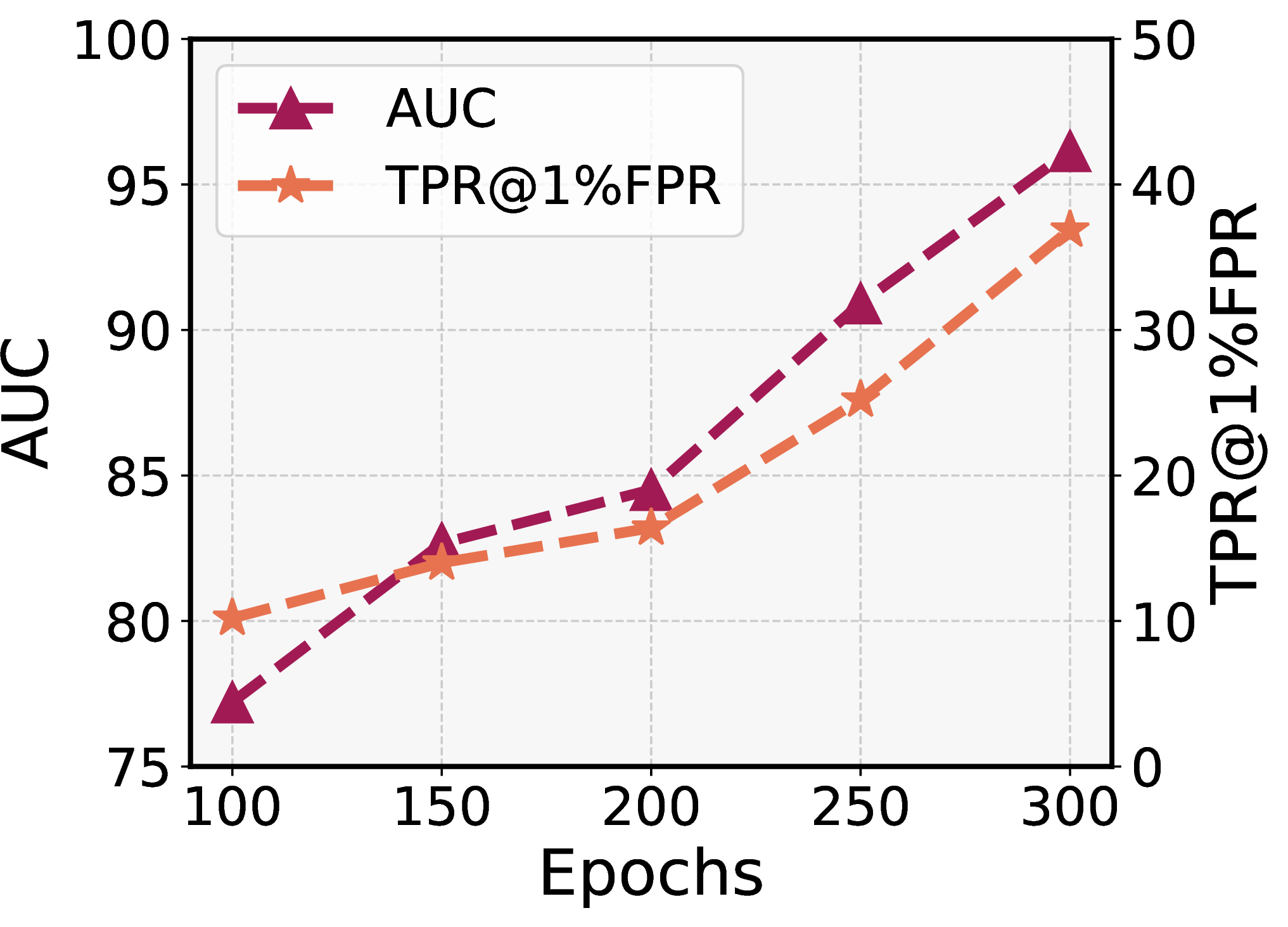
Figure 10: Attack performance across different fine-tuning epochs. Even with only a few fine-tuning epochs, our method yields good results. As the number of epochs increases, its attack performance improves progressively.. a — Pokemon., b — MS-COCO.
9.9 Different Inference↩︎
In real-world scenarios, the number of inference steps of the target model varies depending on the model owner’s configuration. We investigate how different inference steps affect our attack performance, evaluating our method on different datasets with 25, 50, 100, and 200 steps. As shown in Tab. 16, the attack performance exhibits an upward trend as the number of inference steps increases. These results demonstrate that our method consistently achieves strong performance across different inference settings, while further benefiting from longer inference.
| Pokémon | T-to-I | MS-COCO | Flickr | ||||||
|---|---|---|---|---|---|---|---|---|---|
| 2-3 (lr)4-5 (lr)6-7 (lr)8-9 | AUC | T@F=1% | AUC | T@F=1% | AUC | T@F=1% | AUC | T@F=1% | |
| Step=25 | 76.96 | 13.60 | 89.02 | 21.60 | 86.56 | 20.20 | 74.36 | 15.00 | |
| Step=50 | 82.44 | 14.00 | 89.24 | 21.60 | 90.46 | 21.80 | 76.23 | 16.00 | |
| Step=100 | 78.56 | 13.89 | 90.88 | 22.00 | 92.20 | 22.40 | 77.56 | 17.33 | |
| Step=200 | 78.88 | 13.79 | 90.93 | 22.00 | 92.68 | 22.40 | 77.88 | 17.20 | |
9.10 Time overhead↩︎
We compare the time costs of different methods on the Flickr dataset, where the algorithm performs membership inference on a total of 2,000 samples. As shown in Tab. 17, the results indicate that our method achieves the lowest time cost and the highest efficiency.
| Method | NA-P | GD | Feature-T | Feature-C | Feature-D | Ours |
|---|---|---|---|---|---|---|
| Time | \(\approx13h\) | \(\approx9.3h\) | \(\approx13.7h\) | \(\approx13.8h\) | \(\approx13.7h\) | \(\approx8h\) |
| \(SS_{e_i}\) | DataAug | SecMI | PIA | NA-P | GD | Feature-T | Feature-C | Feature-D | Ours | |
|---|---|---|---|---|---|---|---|---|---|---|
| \(\times\) | \(\times\) | 16.99 | 6.40 | 5.57 | 1.00 | 4.00 | 14.60 | 3.60 | 22.90 | |
| \(\times\) | \(✔\) | 16.79 | 5.20 | 5.20 | 1.00 | 3.20 | 14.60 | 3.20 | 21.80 | |
| \(✔\) | \(\times\) | 2.10 | 3.20 | 4.00 | 1.00 | 3.20 | 13.40 | 3.00 | 18.00 | |
| \(✔\) | \(✔\) | 1.90 | 1.50 | 4.00 | 1.00 | 3.20 | 13.20 | 2.60 | 17.90 |
9.11 Impact of Defense↩︎
We present in Tab. 18 the T@F=1% of different methods after applying defense measures. The experimental results demonstrate that our method achieves the best performance under these defenses
9.12 Some Shadow Model-Based Attacks↩︎
Shadow model-based attacks require access to the architectural information of the target model and a partial auxiliary dataset to train the shadow model. As we mentioned in Sec. 1, such attacks suffer from excessive reliance on the quality of the auxiliary dataset. We evaluated two shadow model-based baseline attacks on the Stable Diffusion v1-4 model fine-tuned with the MS-COCO dataset. To investigate the influence of auxiliary data, we employed three different auxiliary datasets (MS-COCO, Flickr, and Pokémon), which exhibit progressively larger distributional gaps from the original fine-tuned data. The experimental results, shown in Fig. 11, indicate that the attack performance declines notably as the distribution of the auxiliary dataset diverges further from that of the fine-tuning data.
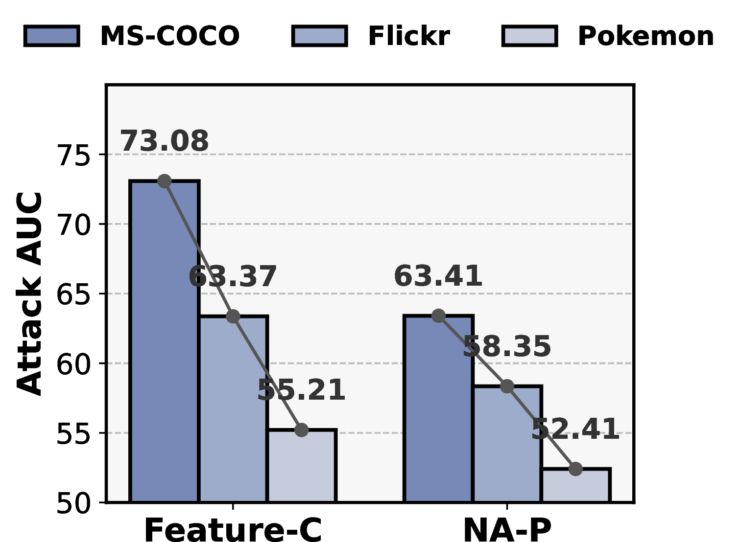
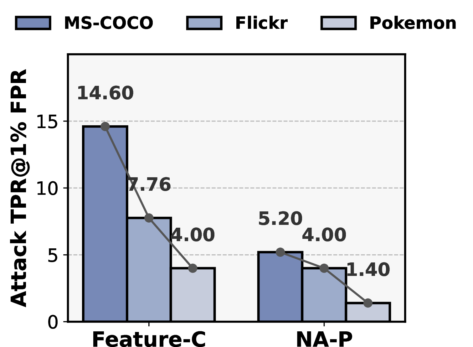
Figure 11: Some shadow model-based attacks’ performance with different auxiliary datasets. The results show that attacks depend heavily on the distribution similarity between the auxiliary and fine-tuned data. As the distribution gap increases, their performance drops significantly.. a — AUC results., b — T@F=1% results.
10 Limitations and Future Works.↩︎
This paper primarily focuses on membership inference attacks on fine-tuned diffusion models, highlighting the crucial role of initial noise in these attacks. Given that initial noise is widely used in noise engineering and image editing tasks, its potential privacy risks deserve greater attention. However, membership inference attacks on pre-trained models have not been sufficiently addressed. Therefore, future research should further explore attack methods and defense strategies for pre-trained models.
11 Impact Statement↩︎
This study introduces a novel membership inference attack aimed at enhancing the ability to determine whether specific samples were used in the training of diffusion models. Membership inference attacks play a crucial role in auditing unauthorized data usage and serve as a key approach to protecting intellectual property. Our method is expected to contribute to advancements in both copyright protection and model privacy research within the domain of image generation. At the same time, we acknowledge that such techniques may also pose potential privacy risks to existing diffusion models. To mitigate misuse, all experiments in this work are conducted on publicly available datasets and open-source model architectures. Furthermore, we will make the implementation of our method publicly accessible.