Dual-Prototype Disentanglement: A Context-Aware Enhancement Framework for Time Series Forecasting
January 01, 1970
Abstract
Time series forecasting has witnessed significant progress with deep learning. While prevailing approaches improve forecasting performance by modifying architectures or introducing novel enhancement strategies, they often fail to dynamically disentangle and leverage the complex, intertwined temporal patterns inherent in time series, thus resulting in the learning of static, averaged representations that lack context-aware capabilities. To address this, we propose the Dual-Prototype Adaptive Disentanglement framework (DPAD), a model-agnostic auxiliary method that equips forecasting models with the ability of pattern disentanglement and context-aware adaptation. Specifically, we construct a Dynamic Dual-Prototype bank (DDP), comprising a common pattern bank with strong temporal priors to capture prevailing trend or seasonal patterns, and a rare pattern bank dynamically memorizing critical yet infrequent events, and then an Dual-Path Context-aware routing (DPC) mechanism is proposed to enhance outputs with selectively retrieved context-specific pattern representations from the DDP. Additionally, we introduce a Disentanglement-Guided Loss (DGLoss) to ensure that each prototype bank specializes in its designated role while maintaining comprehensive coverage. Comprehensive experiments demonstrate that DPAD consistently improves forecasting performance and reliability of state-of-the-art models across diverse real-world benchmarks.
<ccs2012> <concept> <concept_id>10010147.10010178</concept_id> <concept_desc>Computing methodologies Artificial intelligence</concept_desc> <concept_significance>500</concept_significance> </concept> </ccs2012>
1 sec:Introduction↩︎
Time series forecasting (TSF) plays a pivotal role across numerous real-world domains, including weather forecasting [1], [2], transportation scheduling [3], [4], healthcare monitoring [5], [6], energy consumption [7], [8] and finance [9], [10]. Due to the inherent non-stationarity and dynamics, traditional methods fail to effectively model intricate patterns across different time [11], [12]. Recent advances in deep learning have demonstrated a strong capability for capturing intricate temporal dependencies in time series, making it a formidable tool for TSF [13], [14].
Prevailing research focuses on improving forecasting performance by modifying architectures [15], [16] or incorporating novel enhancement strategies [17], [18], both of which have obviously improved the ability to model intricate nonlinear patterns [19], [20]. To effectively capture complex temporal dependencies, some approaches have refined attention mechanisms [21] or redesigned MLP and CNN architectures for improved modeling of long-range and cross-channel dependencies [22], [23]. Meanwhile, some methods introduce enhancement strategies that directly encode prior knowledge about temporal structure into the learning process, which include explicit decomposition schemes that separate trend and seasonal components, as well as techniques such as post-processing to mitigate distribution shifts [24], [25].
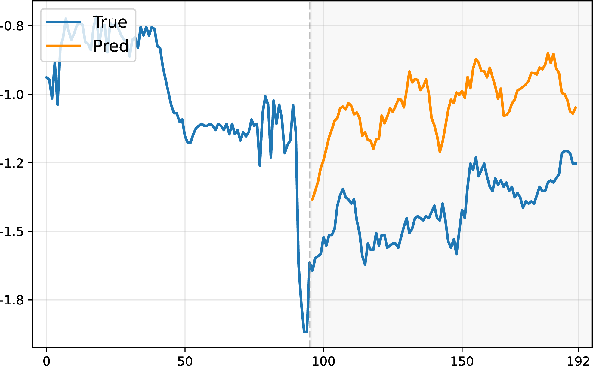
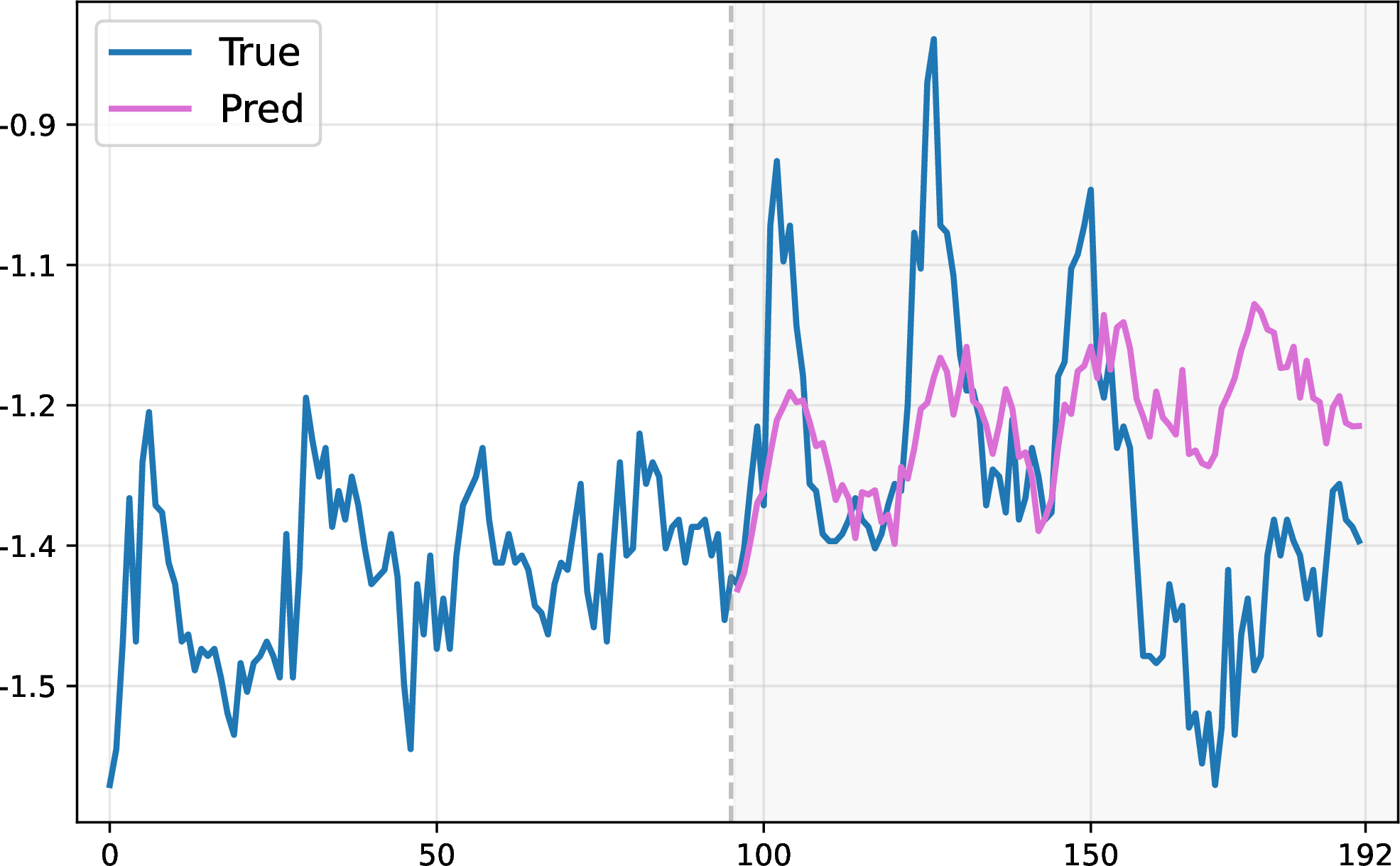
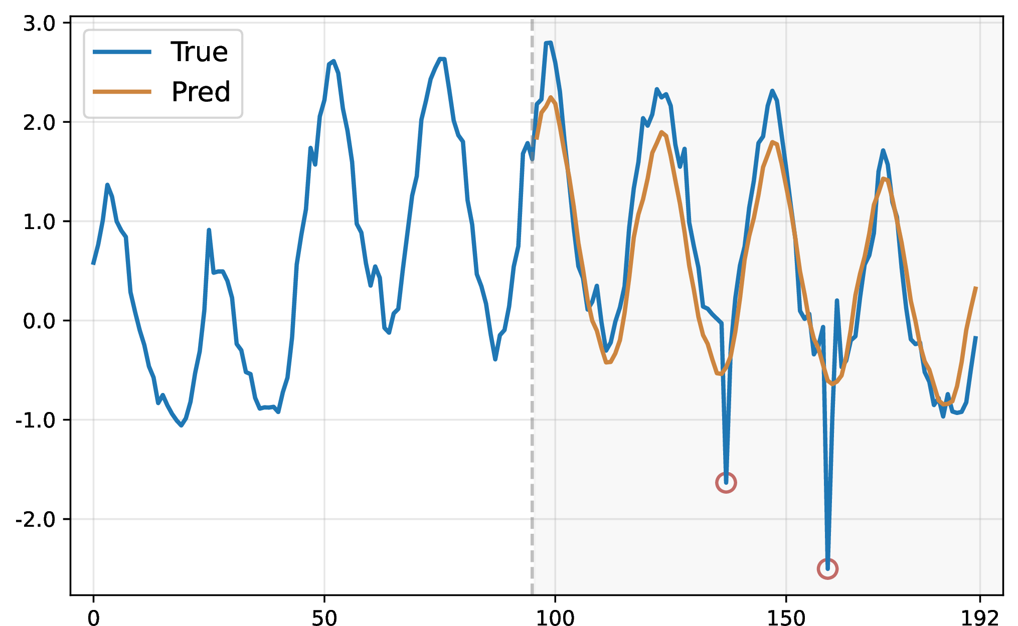
Figure 1: Limitation of static and averaged representations in time series forecasting. We visualize three characteristic failure scenarios where some methods fall short: (a) abrupt distribution shifts, (b) intertwined complex patterns, and (c) critical rare events. These limitations motivate our proposed context-aware enhancement framework.. a — Failure under Distribution Shifts, b — Failure on Intertwined Patterns, c — Failure without Rare Events
Despite these advancements, TSF remains challenging due to the inherent complexity in real-world time series data [26]. This complexity stems primarily from the intrinsic non-stationarity and dynamics, leading to gradual or abrupt distribution shifts over time [27]. Consequently, the learned representations by models may suffer from temporal lag. Meanwhile, time series often exhibit intertwined and complex patterns(e.g., trends, seasonality, and irregular fluctuations) [28], whose influences may vary across different periods and data [29]. In these patterns, some critical yet rare patterns occur infrequently in historical observations, resulting in long-tail distributions that models often fail to adequately memorize [25]. These inherent challenges drive existing methods toward learning averaged, static representations, thereby hindering their ability to capture complex and context-sensitive temporal dependencies [30], [31]. To better illustrate this limitation, we select three representative real-world forecasting scenarios. As shown in Figure 1, a model relying on such representations may struggle to adapt and disentangle individual patterns when confronted with distribution shifts and complex intertwined patterns. This phenomenon underscores the necessity of enhancing the model’s capability for dynamic disentanglement and adaptation to diverse temporal patterns.
To this end, we propose the Dual-Prototype Adaptive Disentanglement framework (DPAD), a novel, model-agnostic paradigm designed to overcome the limitation of static representations by endowing models with context-aware pattern disentanglement capabilities. Unlike prior works that modify the core architecture, DPAD functions as a plug-and-play auxiliary method that can be seamlessly integrated into various forecasting backbones. Specifically, our framework first establishes a learnable Dynamic Dual-Prototype bank (DDP), which comprises a common pattern bank covering prevalent and stable temporal modes, and a rare pattern bank dedicated to memorizing infrequent yet critical events. Then, a Dual-Path Context-aware routing (DPC) mechanism dynamically retrieves and activates relevant patterns from the DDP, thereby enhancing the backbone’s representation via a weighted gating strategy. Furthermore, our framework is optimized with a Disentanglement-Guided Loss (DGLoss) that jointly ensures the separation of common and rare patterns, enforces diversity among common prototypes, and maintains the distinctiveness of rare prototypes. Our contributions are summarized as follows:
We introduce a novel context-aware enhancement framework based on dual-prototype disentanglement. Unlike existing methods, our framework equips models with the capability for context-aware and pattern disentanglement, thereby directly mitigating the inherent limitation of static representations and enhancing their ability to dynamically model intricate temporal patterns.
We propose DPAD, a model-agnostic auxiliary framework that employs a learnable dual-prototype bank and an adaptive routing mechanism to dynamically enhance model’s prediction. A disentanglement-guided loss is further introduced to enforce effective pattern separation and preservation, which jointly optimizes the backbone and the prototype banks.
Comprehensive experiments on multiple real-world datasets and state-of-the-art backbones demonstrate that DPAD consistently enhances forecasting performance with only negligible computational overhead.
2 Related Work↩︎
2.1 Time Series Forecasting Models↩︎
Recent years have witnessed remarkable progress in deep forecasting models, with their core advancement lying in learning more expressive temporal representations [32], [33]. Existing models can be broadly categorized by architecture into MLP-based, CNN-based, Transformer-based, and LLM-based approaches [11]. MLP-based architectures [22], [34], [35] often employ decomposition strategies and simple linear layers to capture cross-time dependencies, offering a compelling balance of efficiency and performance. CNN-based architectures [36]–[38] leverage hierarchical convolution structures and frequency-domain analysis [15] to model local patterns and multi-periodicity effectively. Nevertheless, both of them often struggle to capture long-term dependencies. Therefore, Transformer-based architectures [39]–[41] have emerged as a powerful paradigm by introducing various efficient attention mechanisms to capture global dependencies. More recently, LLM-based approaches [42]–[44] have explored adapting pre-trained large language models for time series forecasting, leveraging their massive parameters and in-context learning capabilities. While excelling at capturing stable, recurring patterns, these models often tend to converge to a flexible representation [45], [46]. Consequently, they struggle to adaptively disentangle representations in response to the specific context of input sequences, such as distribution shifts, intricate mixtures of patterns, or the emergence of anomalies. This inherent rigidity underscores the need for a complementary mechanism that can inject contextual adaptability into these models.
2.2 Enhancement Strategies for Time Series Forecasting↩︎
Beyond architectural innovations, several efficient and model-agnostic strategies have been proposed to enhance predictive performance. Some methods employ decomposition strategies as a strong inductive bias to guide model in handling diverse temporal patterns more effectively [13], [47]. Autoformer [16] decomposes time series into seasonal and trend components, allowing other models to handle input from a clearer perspective. TimesNet [15] learns frequency-adaptive periods in the frequency domain to explicitly model intra- and inter-period variations. Another strategy focuses on model-agnostic methods [24], [48]. RAFT [27] employs retrieval augmented generation to retrieve from historical samples, providing the model with relevant information. HCAN [49] assigns class labels for timesteps to equip models with contextual-aware capability. Furthermore, specialized loss function designs have been designed to improve robustness against distribution shifts and intricate patterns [25], [46]. DBLoss [31] decomposes both predictions and ground truth to calculate the loss for each component separately. PSLoss [30] enhances structural alignment by comparing time series at the patch level with statistical properties. While these strategies improve forecasting performance, they still fail to dynamically disentangle complex, intertwined patterns in a context-aware manner. Different from them, our proposed DPAD framework introduces a learnable dual-prototype bank and adaptively fuses them through a context-aware routing mechanism, thereby enabling dynamic and interpretable enhancement of the backbone model’s representations with high efficiency.
3 Method↩︎
Time series forecasting addresses the fundamental challenge of predicting future values \({Y} = {y_{t+1}, ..., y_{t+h}} \in \mathbb{R}^{h\times{C}}\) from historical observations \({X} = {x_1, ..., x_t} \in \mathbb{R}^{t\times{C}}\), where \(h\) is the prediction horizon, \(t\) is the history horizon, and \(C\) is the number of variables.
3.1 Structure Overview↩︎
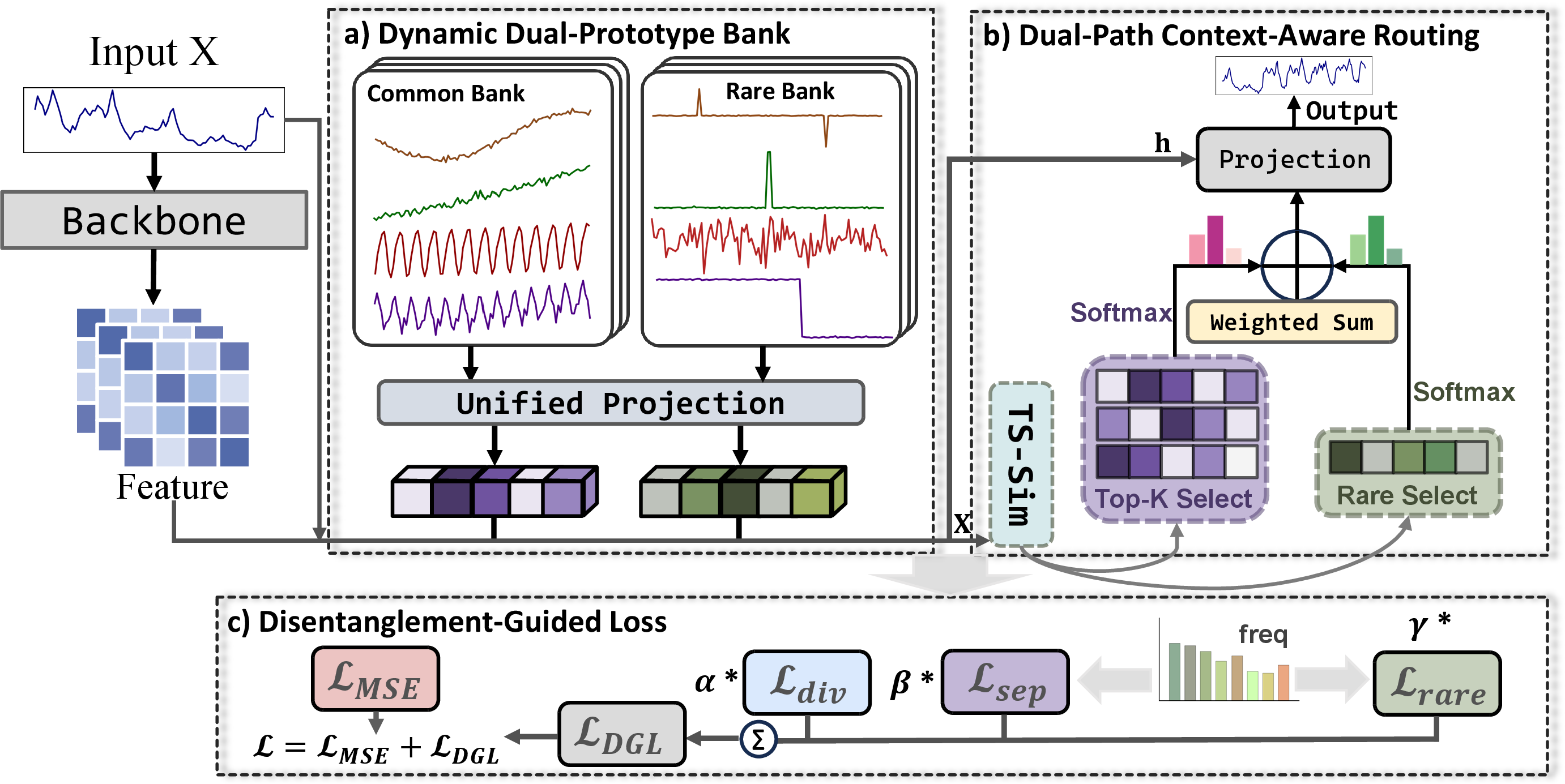
As illustrated in Figure 2, our proposed DPAD consists three key components: (a) Dynamic Dual-Prototype Bank (DDP) that maintains a set of common and rare pattern prototypes to explicitly disentangle different patterns and dynamically update; (b) Dual-Path Context-aware routing (DPC) that dynamically retrieves and activates relevant prototypes from DDP, in which the representation is generated by an arbitrary backbone model, and then enhances the prediction through a weighted gating strategy; (c) Disentanglement-Guided Loss (DGLoss) that jointly optimizes DDP and the backbone model through a quadruple loss formulation, which ensures both the specialization and separation of the prototypes.
3.2 Dynamic Dual-Prototype Bank↩︎
The Dynamic Dual-Prototype bank (DDP) serves as the cornerstone of our framework, designed to explicitly disentangle and memorize two distinct categories of temporal patterns: prevalent common patterns and critical yet infrequent rare patterns. Formally, the DDP consists of two separate prototype sets: a Common Pattern Bank \(\mathcal{B}_c\), which comprises sequences synthesized from a combination of fundamental trends and seasonal patterns, and a Rare Pattern Bank \(\mathcal{B}_r\), dedicated to memorizing long-tailed, sudden events and some other temporal noise.
Specifically, we generate two groups of base sequences \(\{\mathbf{s}_c^{i}\}\) and rare sequences \(\{\mathbf{s}_r^{j}\}\) using distinct prior strategies to reflect their different pattern characteristics: \[\mathbf{s}_c^{i} \sim \mathcal{GP}\left(0, \, \lambda_{\text{l}} K_{\text{l}} + \lambda_{\text{r}} K_{\text{r}} + \lambda_{\text{p}} K_{\text{p}}\right),\quad i=1,\dots,M,\] \[\mathbf{s}_r^{j} \sim \mathcal{N}(0, \sigma^2 \mathbf{I}),\quad j=1,\dots,N,\] where \(\mathbf{s}_c^{i}\) denotes the common sequences generated via a mixture of Gaussian Process \(\mathcal{GP}\) kernels to embed strong temporal priors, and \(K_{\text{l}}, K_{\text{r}}, K_{\text{p}}\) are the Linear, radial basis function (RBF), and Periodic kernel, \(\lambda_i\) is mixing coefficients. This strategy yields diverse yet structured prototypes that cover stable, recurring patterns such as trends, seasonality, and their mixtures, thereby providing a well-initialized basis for modeling prevalent temporal dynamics.
In contrast, \(\mathbf{s}_r^{j}\) is initialized from a Gaussian distribution \(\mathcal{N}(0, \sigma^2 \mathbf{I})\), where \(\sigma^2\) is a small variance controlling the magnitude of initialization noise. This minimal random initialization ensures that rare prototypes begin from a nearly unbiased state, allowing them to remain flexible and exclusively adapt to capture rare patterns during training, without being predisposed to common modes. Notably, all of sequence sets would be transformed into learnable parameters.
Then each generated sequence is projected into a shared \(D\)-dimensional latent space via the linear layers: \[\mathbf{p}_c^{i} = \mathbf{Proj}_c(\mathbf{s}_c^{i}),\] \[\mathbf{p}_r^{j} = \mathbf{Proj}_r(\mathbf{s}_r^{j}),\]
The resulting Common Pattern Bank \(\mathcal{B}_c\) and Rare Pattern Bank \(\mathcal{B}_r\) are defined as follows: \[\mathcal{B}_c = \{\mathbf{p}_c^{1}, \mathbf{p}_c^{2},\dots,\mathbf{p}_c^{M}\},\quad \mathcal{B}_r = \{\mathbf{p}_r^{1}, \mathbf{p}_r^{2},\dots,\mathbf{p}_r^{N}\},\] This strategy explicitly separates the modeling of common and rare patterns while keeping the prototype representation compact and adaptive. Both \(\mathcal{B}_c\) and \(\mathcal{B}_r\) are updated throughout training via the disentanglement loss described in 3.4. This allows the common prototypes to evolve toward more representative and dataset-specific stable patterns, while the rare prototypes dynamically adapt to capture and memorize infrequent yet critical temporal patterns.
3.3 Dual-Path Context-Aware Routing↩︎
Dual-Path Context-aware routing (DPC) mechanism is proposed to adaptively enhance final prediction. Given the input \(\mathbf{X}\) and its contextual representation \(\mathbf{h} \in \mathbb{R}^D\) from the backbone model, our DPC dynamically retrieves and fuses relevant patterns from the DDP through a dual-path design using TS-Sim block. Specifically, we first project \(\mathbf{X}\) into the same \(D\)-dimensional latent space as the prototypes via a learnable linear projection \(\phi\). Then we compute the similarity scores \(\mathbf{\rho}_c\) and \(\mathbf{\rho}_r\) between the input \(\mathbf{X}\) and each prototype in \(\mathcal{B}_c\) and \(\mathcal{B}_r\) in the latent space: \[\mathbf{\rho}_c = s(\phi{(\mathbf{X})}, \mathcal{B}_c),\quad \mathbf{\rho}_r = s(\phi{(\mathbf{X})}, \mathcal{B}_r),\] Here we adopt the Pearson Correlation as the similarity measurement \(s(\cdot, \cdot)\), which provides scale-invariant matching that focuses on the shape similarity of temporal patterns. We then employ a dual-path selection strategy to retrieve the most relevant prototypes: \[\mathcal{I}_c = \arg \text{top-K}(\mathbf{\rho}_i|1<i\leq K),\] \[\mathcal{I}_r = \begin{cases} \arg \max (\rho_r), & \text{if } \max(\rho_r) > \epsilon \\ \varnothing, & \text{otherwise} \end{cases}\] For the common bank \(\mathcal{B}_c\), we select \(\text{top-K}\) prototypes with the highest similarity scores, forming an index set \(\mathcal{I}_c\). Conversely, to enforce sparsity and precise memory for rare events, we select at most one prototype from the rare bank \(\mathcal{B}_r\), with its index denoted as \(\mathcal{I}_r\).
Then we compute adaptive weights for the selected common and rare prototypes by Softmax function: \[\omega_c = \text{Softmax}(\rho_c[\mathcal{I}_c] / \tau),\quad \omega_r = \text{Softmax}(\rho_r[\mathcal{I}_r] / \tau),\] Then the retrieved pattern contributions are then computed as weighted sums: \[\mathbf{z}_c = \sum_{k \in \mathcal{I}_c}\omega_c^{k} \cdot \mathcal{B}_c[\mathcal{I}_c], \quad \mathbf{z}_r = \omega_r \cdot \mathcal{B}_r[\mathcal{I}_r],\] Finally, these context-aware contributions are fused with the backbone representation \(\mathbf{h}\) through concatenation and a linear projection to produce the enhanced prediction \(\mathbf{Y}\): \[\mathbf{Y} = \mathbf{W}_o [\mathbf{h}; \mathbf{z}_c; \mathbf{z}_r],\] This adaptive fusion mechanism thereby enhances the capability of the model to dynamically disentangle intricate temporal dependencies, which mitigates the inherent limitation of static, averaged representations.
3.4 Disentanglement-Guided Loss↩︎
To ensure the DDP learns a well-disentangled and effective representation of common and rare patterns, we propose a Disentanglement-Guided Loss (DGLoss). This loss function jointly optimizes the parameters of backbone model and the DDP by enforcing three key properties: pattern separation, rarity preservation, and common set diversity.
We first introduce the Separation Loss \(\mathcal{L}_{\text{sep}}\) to ensure a clear functional divide between the common and rare banks, preventing role confusion. Guided by pattern frequency statistics within a training batch, \(\mathcal{L}_{\text{sep}}\) dynamically encourages each bank to specialize in its respective domain: \[\mathcal{L}_{\text{sep}} = \mathbb{E}[\omega\cdot max(0, m - \triangle{\mathbf{\rho}}) + (1-\omega)\cdot max(0, m + \triangle{\mathbf{\rho}})],\] where \(\triangle{\mathbf{\rho}}\) is the difference between similarities \(\mathbf{\rho}_c\) and \(\mathbf{\rho}_r\), \(m\) is a margin, and \(\omega \in [0,1]\) is a frequency weight that computed as the exponential moving average of prototypes activation frequencies across batches. Intuitively, if the input contains patterns frequently observed in recent batches, \(\mathcal{L}_{\text{sep}}\) penalizes activation of the rare bank, while for a rare input pattern, it penalizes over-reliance on the common bank.
Then we propose a Rarity Preservation Loss \(\mathcal{L}_{\text{rare}}\). With the contrastive restriction, \(\mathcal{L}_{\text{rare}}\) prevents the prototypes in the rare bank from being contaminated or forgotten due to common patterns, thereby ensuring their persistent memory for rare patterns: \[\mathcal{L}_{\text{rare}} = -\frac{1}{|\mathcal{A}|} \sum_{k\in\mathcal{A}} \log[ \frac{\exp(\frac{s_{kk}}{\tau})}{\sum_{j=1}^N \exp(\frac{s_{kj}}{\tau}) }],\] where \(\mathcal{A}\) is the set of activated rare prototype indices for the input, \(s_{kj}\) denotes the similarity between the input representation and the \(j\)-th rare prototype. \(\mathcal{L}_{\text{rare}}\) pulls the input representation closer to the activated rare prototype in the latent space while pushing it away from other rare prototypes.
Furthermore, we adopt a diversity loss \(\mathcal{L}_{\text{div}}\) that leverages orthogonal constraints to promote diversity and reduce redundancy among common prototypes, thereby ensuring the common bank covers a more comprehensive range of prevalent patterns: \[\mathcal{L}_{\text{div}} = \frac{1}{M(M-1)} \sum_{i=1}^{M} \sum_{j \neq i}^{M} \left( \frac{ {\mathbf{p}_c^{i}}^\top \mathbf{p}_c^{j} }{ \|\mathbf{p}_c^{i}\| \|\mathbf{p}_c^{j}\| } \right)^2,\] where \(M\) is the number of common prototypes and \(\mathbf{p}_c^i\) is the \(i\)-th common prototype vector.
Finally, we integrated this three loss terms as the Disentanglement-Guided Loss \(\mathcal{L}_{\text{DGL}}\): \[\mathcal{L}_{\text{DGL}} = \lambda_\text{sep} \mathcal{L}_{\text{sep}} + \lambda_\text{rare} \mathcal{L}_{\text{rare}} + \lambda_\text{div} \mathcal{L}_{\text{div}},\] where \(\lambda_\text{sep}, \lambda_\text{rare}, \lambda_\text{div}\) are balancing coefficients. The total loss function is formulated as follows: \[\mathcal{L} = \mathcal{L}_\text{MSE} + \mathcal{L}_\text{DGL}\] By explicitly coordinating the separation, preservation, and diversity of temporal prototypes, our DGLoss shapes a well-structured and disentangled pattern memory. This mechanism enables the model to dynamically retrieve context-aware patterns, effectively mitigating the limitation of static representation.
4 Experiments↩︎
To comprehensively verify the performance and effectiveness of the proposed DPAD, we conduct extensive experiments on both long-term and short-term forecasting tasks.
4.1 Experimental Setup↩︎
4.1.1 Datasets.↩︎
We conduct long-term forecasting experiments on 6 real-world datasets, including (1) ETT (ETTh1, ETTh2, ETTm1, ETTm2) contains 7 features of electricity transformer data from July 2016 to July 2018, which was sampled at hourly (ETTh1, ETTh2) and 15-minute (ETTm1, ETTm2) intervals. (2) Electricity (ECL) records hourly electricity consumption data of 321 clients from 2012 to 2014. (3) Exchange collects the daily exchange-rate data from eight different countries. (4) Solar-Energy contains the solar power production of 137 PV plants in 2006, which is sampled every 10 minutes. (5) Weather includes 21 meteorological factors collected every 10 minutes from the Max Planck Biogeochemistry Institute’s Weather Station in 2020. (6) Traffic contains hourly road occupancy rates from 862 sensors on San Francisco freeways. Meanwhile, we conduct short-term forecasting experiments on PEMS (PEMS03, PEMS04, PEMS07, PEMS08), which contains the public traffic network data in California with a 5-minute interval. The details of datasets are listed in Table 1.
| Name | Domain | Length | Num | Prediction Length | Dataset Size | Freq. (m) |
|---|---|---|---|---|---|---|
| ETTh1 | Temperature | 14400 | 7 | {96,192,336,720} | (8545,2881,2881) | 60 |
| ETTh2 | Temperature | 14400 | 7 | {96,192,336,720} | (8545,2881,2881) | 60 |
| ETTm1 | Temperature | 57600 | 7 | {96,192,336,720} | (34465,11521,11521) | 15 |
| ETTm2 | Temperature | 57600 | 7 | {96,192,336,720} | (34465,11521,11521) | 15 |
| Electricity | Electricity | 26304 | 321 | {96,192,336,720} | (18317,2633,5261) | 60 |
| Exchange | Exchange Rate | 7588 | 8 | {96,192,336,720} | (5120,665,1422) | 1440 |
| Traffic | Road Occupancy | 17544 | 862 | {96,192,336,720} | (12185,1757,3509) | 60 |
| Weather | Weather | 52696 | 21 | {96,192,336,720} | (36792,5271,10540) | 10 |
| Solar-Energy | Energy | 52179 | 137 | {96,192,336,720} | (36601,5161,10417) | 10 |
| PEMS03 | Traffic Flow | 26208 | 358 | {12,24,48,96} | (15617,5135,5135) | 5 |
| PEMS04 | Traffic Flow | 16992 | 307 | {12,24,48,96} | (10172,3375,3375) | 5 |
| PEMS07 | Traffic Flow | 28224 | 883 | {12,24,48,96} | (16711,5622,5622) | 5 |
| PEMS08 | Traffic Flow | 17856 | 170 | {12,24,48,96} | (10690,3548,3548) | 5 |
4.1.2 Baselines.↩︎
To verify the performance and effectiveness of our DPAD, we select five state-of-the-art (SOTA) time series forecasting models with diverse architectures, including transformer-based models: iTransformer [21], TimeXer [26], TimeBridge [41]; MLP-based models: DLinear [45]; and CNN-based models: TimesNet [15].
4.1.3 Implementation Details.↩︎
All experiments are implemented in PyTorch, and conducted on a single NVIDIA RTX 4090 24 GB GPU. We utilize ADAM optimizer with an initial learning rate \(10^{-3}\) and L2 loss for model optimization. For fair evaluation, we use the framework of TimesNet [15], and all the baselines are implemented based on the configurations of original paper and its code.
4.1.4 Metrics Details.↩︎
To evaluate forecasting performance for TSF, we utilize the mean square error (MSE) and mean absolute error (MAE). The calculations of metrics are as follows: \[\label{metrics32MSE} \boldsymbol{MSE} = \frac{1}{n}\sum_{i=1}^{n}(\mathbf{Y}_i - \hat{\mathbf{Y}}_i)^2, \quad \boldsymbol{MAE} = \frac{1}{n}\sum_{i=1}^{n}|\mathbf{Y}_i - \hat{\mathbf{Y}}_i|.\tag{1}\]
| Methods | iTransformer | DLinear | TimesNet | TimeXer | TimeBridge | ||||||||||||||||
|---|---|---|---|---|---|---|---|---|---|---|---|---|---|---|---|---|---|---|---|---|---|
| 3-22 | Ori | +DPAD | Ori | +DPAD | Ori | +DPAD | Ori | +DPAD | Ori | +DPAD | |||||||||||
| Metric | MSE | MAE | MSE | MAE | MSE | MAE | MSE | MAE | MSE | MAE | MSE | MAE | MSE | MAE | MSE | MAE | MSE | MAE | MSE | MAE | |
| 96 | 0.387 | 0.405 | 0.383 | 0.401 | 0.397 | 0.412 | 0.388 | 0.403 | 0.415 | 0.429 | 0.419 | 0.423 | 0.386 | 0.404 | 0.379 | 0.398 | 0.377 | 0.395 | 0.371 | 0.388 | |
| 192 | 0.441 | 0.436 | 0.433 | 0.423 | 0.446 | 0.441 | 0.431 | 0.432 | 0.479 | 0.466 | 0.471 | 0.460 | 0.429 | 0.435 | 0.433 | 0.430 | 0.427 | 0.425 | 0.423 | 0.421 | |
| 336 | 0.494 | 0.463 | 0.478 | 0.452 | 0.489 | 0.467 | 0.478 | 0.459 | 0.517 | 0.482 | 0.504 | 0.473 | 0.484 | 0.457 | 0.472 | 0.446 | 0.477 | 0.456 | 0.461 | 0.441 | |
| 720 | 0.488 | 0.483 | 0.492 | 0.482 | 0.513 | 0.511 | 0.501 | 0.506 | 0.505 | 0.490 | 0.512 | 0.496 | 0.544 | 0.513 | 0.483 | 0.493 | 0.521 | 0.498 | 0.473 | 0.474 | |
| Avg | 0.452 | 0.446 | 0.446 | 0.439 | 0.461 | 0.457 | 0.449 | 0.450 | 0.479 | 0.466 | 0.476 | 0.463 | 0.460 | 0.452 | 0.442 | 0.441 | 0.450 | 0.443 | 0.432 | 0.431 | |
| 96 | 0.301 | 0.350 | 0.293 | 0.345 | 0.341 | 0.394 | 0.332 | 0.381 | 0.316 | 0.358 | 0.309 | 0.358 | 0.284 | 0.337 | 0.276 | 0.331 | 0.294 | 0.345 | 0.287 | 0.333 | |
| 192 | 0.380 | 0.399 | 0.374 | 0.393 | 0.482 | 0.479 | 0.466 | 0.471 | 0.415 | 0.414 | 0.397 | 0.407 | 0.366 | 0.391 | 0.366 | 0.392 | 0.377 | 0.395 | 0.359 | 0.380 | |
| 336 | 0.423 | 0.431 | 0.416 | 0.425 | 0.591 | 0.541 | 0.535 | 0.512 | 0.452 | 0.448 | 0.433 | 0.436 | 0.438 | 0.438 | 0.424 | 0.429 | 0.424 | 0.433 | 0.408 | 0.418 | |
| 720 | 0.431 | 0.447 | 0.422 | 0.435 | 0.839 | 0.661 | 0.785 | 0.638 | 0.461 | 0.463 | 0.448 | 0.455 | 0.407 | 0.449 | 0.411 | 0.432 | 0.423 | 0.442 | 0.417 | 0.435 | |
| Avg | 0.383 | 0.406 | 0.376 | 0.399 | 0.563 | 0.518 | 0.529 | 0.500 | 0.411 | 0.420 | 0.396 | 0.414 | 0.373 | 0.403 | 0.369 | 0.396 | 0.379 | 0.403 | 0.367 | 0.391 | |
| 96 | 0.341 | 0.376 | 0.332 | 0.369 | 0.346 | 0.374 | 0.334 | 0.369 | 0.336 | 0.375 | 0.329 | 0.371 | 0.318 | 0.356 | 0.320 | 0.358 | 0.324 | 0.362 | 0.311 | 0.345 | |
| 192 | 0.382 | 0.396 | 0.377 | 0.389 | 0.382 | 0.391 | 0.375 | 0.392 | 0.377 | 0.395 | 0.376 | 0.393 | 0.373 | 0.389 | 0.366 | 0.383 | 0.365 | 0.384 | 0.361 | 0.375 | |
| 336 | 0.420 | 0.421 | 0.411 | 0.412 | 0.415 | 0.415 | 0.405 | 0.415 | 0.418 | 0.420 | 0.405 | 0.409 | 0.412 | 0.387 | 0.407 | 0.394 | 0.398 | 0.407 | 0.392 | 0.397 | |
| 720 | 0.487 | 0.456 | 0.484 | 0.451 | 0.473 | 0.451 | 0.465 | 0.443 | 0.541 | 0.481 | 0.493 | 0.464 | 0.460 | 0.450 | 0.451 | 0.441 | 0.462 | 0.444 | 0.455 | 0.431 | |
| Avg | 0.407 | 0.412 | 0.401 | 0.405 | 0.404 | 0.407 | 0.394 | 0.404 | 0.418 | 0.417 | 0.400 | 0.409 | 0.390 | 0.395 | 0.386 | 0.394 | 0.387 | 0.399 | 0.379 | 0.387 | |
| 96 | 0.186 | 0.272 | 0.179 | 0.263 | 0.193 | 0.293 | 0.190 | 0.295 | 0.188 | 0.268 | 0.181 | 0.264 | 0.172 | 0.254 | 0.165 | 0.251 | 0.177 | 0.260 | 0.176 | 0.254 | |
| 192 | 0.252 | 0.312 | 0.245 | 0.306 | 0.284 | 0.361 | 0.273 | 0.353 | 0.250 | 0.306 | 0.243 | 0.304 | 0.241 | 0.302 | 0.238 | 0.300 | 0.243 | 0.303 | 0.242 | 0.298 | |
| 336 | 0.315 | 0.351 | 0.309 | 0.344 | 0.382 | 0.429 | 0.367 | 0.415 | 0.306 | 0.341 | 0.298 | 0.337 | 0.301 | 0.340 | 0.397 | 0.331 | 0.303 | 0.342 | 0.304 | 0.338 | |
| 720 | 0.415 | 0.408 | 0.409 | 0.405 | 0.558 | 0.525 | 0.508 | 0.501 | 0.420 | 0.405 | 0.402 | 0.398 | 0.394 | 0.395 | 0.396 | 0.393 | 0.401 | 0.399 | 0.409 | 0.397 | |
| Avg | 0.292 | 0.335 | 0.285 | 0.329 | 0.354 | 0.402 | 0.334 | 0.391 | 0.291 | 0.330 | 0.281 | 0.325 | 0.277 | 0.322 | 0.299 | 0.318 | 0.281 | 0.326 | 0.282 | 0.321 | |
| 96 | 0.148 | 0.241 | 0.147 | 0.234 | 0.211 | 0.302 | 0.202 | 0.293 | 0.163 | 0.267 | 0.159 | 0.269 | 0.241 | 0.244 | 0.141 | 0.241 | 0.143 | 0.239 | 0.135 | 0.228 | |
| 192 | 0.167 | 0.248 | 0.162 | 0.251 | 0.211 | 0.305 | 0.203 | 0.293 | 0.184 | 0.284 | 0.178 | 0.281 | 0.159 | 0.260 | 0.153 | 0.257 | 0.161 | 0.256 | 0.154 | 0.247 | |
| 336 | 0.179 | 0.271 | 0.172 | 0.271 | 0.223 | 0.319 | 0.210 | 0.304 | 0.196 | 0.297 | 0.205 | 0.303 | 0.177 | 0.276 | 0.177 | 0.271 | 0.176 | 0.272 | 0.172 | 0.264 | |
| 720 | 0.208 | 0.298 | 0.201 | 0.289 | 0.258 | 0.351 | 0.243 | 0.332 | 0.232 | 0.325 | 0.243 | 0.331 | 0.229 | 0.321 | 0.210 | 0.306 | 0.204 | 0.297 | 0.201 | 0.288 | |
| Avg | 0.175 | 0.264 | 0.170 | 0.261 | 0.225 | 0.319 | 0.214 | 0.305 | 0.193 | 0.293 | 0.196 | 0.296 | 0.201 | 0.275 | 0.170 | 0.268 | 0.171 | 0.266 | 0.165 | 0.256 | |
| 96 | 0.088 | 0.208 | 0.081 | 0.202 | 0.098 | 0.233 | 0.095 | 0.228 | 0.115 | 0.242 | 0.097 | 0.224 | 0.094 | 0.214 | 0.086 | 0.205 | 0.113 | 0.236 | 0.084 | 0.201 | |
| 192 | 0.180 | 0.303 | 0.175 | 0.299 | 0.186 | 0.325 | 0.182 | 0.319 | 0.216 | 0.333 | 0.186 | 0.310 | 0.182 | 0.303 | 0.179 | 0.301 | 0.200 | 0.327 | 0.177 | 0.297 | |
| 336 | 0.331 | 0.418 | 0.326 | 0.414 | 0.325 | 0.434 | 0.329 | 0.442 | 0.375 | 0.444 | 0.360 | 0.434 | 0.384 | 0.448 | 0.350 | 0.426 | 0.364 | 0.440 | 0.339 | 0.421 | |
| 720 | 0.848 | 0.695 | 0.835 | 0.692 | 0.746 | 0.663 | 0.772 | 0.678 | 0.101 | 0.765 | 0.893 | 0.720 | 0.932 | 0.724 | 0.887 | 0.706 | 0.992 | 0.760 | 0.847 | 0.691 | |
| Avg | 0.361 | 0.406 | 0.354 | 0.401 | 0.338 | 0.413 | 0.345 | 0.417 | 0.201 | 0.446 | 0.384 | 0.422 | 0.398 | 0.422 | 0.375 | 0.409 | 0.417 | 0.440 | 0.361 | 0.402 | |
| 96 | 0.207 | 0.237 | 0.199 | 0.221 | 0.290 | 0.378 | 0.240 | 0.299 | 0.223 | 0.256 | 0.211 | 0.249 | 0.198 | 0.244 | 0.191 | 0.235 | 0.204 | 0.245 | 0.196 | 0.212 | |
| 192 | 0.242 | 0.264 | 0.237 | 0.254 | 0.320 | 0.398 | 0.263 | 0.312 | 0.262 | 0.272 | 0.241 | 0.267 | 0.226 | 0.270 | 0.221 | 0.262 | 0.237 | 0.269 | 0.228 | 0.236 | |
| 336 | 0.251 | 0.277 | 0.249 | 0.273 | 0.353 | 0.415 | 0.279 | 0.314 | 0.287 | 0.299 | 0.257 | 0.291 | 0.239 | 0.281 | 0.231 | 0.275 | 0.251 | 0.283 | 0.247 | 0.256 | |
| 720 | 0.251 | 0.278 | 0.250 | 0.276 | 0.357 | 0.413 | 0.276 | 0.310 | 0.298 | 0.318 | 0.267 | 0.298 | 0.242 | 0.282 | 0.238 | 0.277 | 0.253 | 0.284 | 0.255 | 0.260 | |
| Avg | 0.237 | 0.264 | 0.233 | 0.256 | 0.330 | 0.401 | 0.264 | 0.308 | 0.267 | 0.286 | 0.244 | 0.276 | 0.226 | 0.269 | 0.220 | 0.262 | 0.236 | 0.270 | 0.231 | 0.241 | |
| 96 | 0.393 | 0.269 | 0.392 | 0.268 | 0.712 | 0.438 | 0.647 | 0.402 | 0.593 | 0.317 | 0.471 | 0.295 | 0.428 | 0.271 | 0.415 | 0.263 | 0.375 | 0.270 | 0.371 | 0.243 | |
| 192 | 0.412 | 0.277 | 0.407 | 0.271 | 0.662 | 0.417 | 0.599 | 0.380 | 0.618 | 0.327 | 0.493 | 0.309 | 0.447 | 0.280 | 0.442 | 0.273 | 1.411 | 0.803 | 0.397 | 0.254 | |
| 336 | 0.424 | 0.283 | 0.417 | 0.279 | 0.669 | 0.419 | 0.590 | 0.374 | 0.642 | 0.341 | 0.514 | 0.320 | 0.472 | 0.289 | 0.473 | 0.290 | 1.427 | 0.806 | 0.408 | 0.261 | |
| 720 | 0.459 | 0.301 | 0.447 | 0.293 | 0.709 | 0.437 | 0.616 | 0.385 | 0.679 | 0.350 | 0.568 | 0.351 | 0.517 | 0.307 | 0.522 | 0.310 | 0.435 | 0.298 | 0.602 | 0.387 | |
| Avg | 0.422 | 0.282 | 0.416 | 0.278 | 0.688 | 0.427 | 0.613 | 0.385 | 0.633 | 0.333 | 0.511 | 0.318 | 0.466 | 0.286 | 0.463 | 0.284 | 0.912 | 0.544 | 0.444 | 0.286 | |
| 96 | 0.176 | 0.216 | 0.170 | 0.208 | 0.195 | 0.252 | 0.187 | 0.255 | 0.172 | 0.221 | 0.156 | 0.204 | 0.157 | 0.205 | 0.151 | 0.201 | 0.177 | 0.218 | 0.173 | 0.210 | |
| 192 | 0.225 | 0.257 | 0.223 | 0.256 | 0.239 | 0.299 | 0.228 | 0.291 | 0.220 | 0.260 | 0.207 | 0.249 | 0.204 | 0.248 | 0.202 | 0.244 | 0.223 | 0.258 | 0.216 | 0.251 | |
| 336 | 0.281 | 0.299 | 0.279 | 0.295 | 0.282 | 0.333 | 0.273 | 0.335 | 0.280 | 0.302 | 0.265 | 0.294 | 0.264 | 0.293 | 0.264 | 0.292 | 0.279 | 0.299 | 0.280 | 0.291 | |
| 720 | 0.361 | 0.353 | 0.355 | 0.347 | 0.345 | 0.381 | 0.349 | 0.388 | 0.353 | 0.350 | 0.349 | 0.343 | 0.343 | 0.343 | 0.341 | 0.344 | 0.354 | 0.349 | 0.356 | 0.343 | |
| Avg | 0.260 | 0.281 | 0.256 | 0.276 | 0.265 | 0.316 | 0.259 | 0.317 | 0.256 | 0.283 | 0.244 | 0.272 | 0.242 | 0.272 | 0.239 | 0.270 | 0.258 | 0.281 | 0.256 | 0.273 | |
| Methods | iTransformer | DLinear | TimesNet | TimeXer | TimeBridge | ||||||||||||||||
|---|---|---|---|---|---|---|---|---|---|---|---|---|---|---|---|---|---|---|---|---|---|
| 3-22 | Ori | +DPAD | Ori | +DPAD | Ori | +DPAD | Ori | +DPAD | Ori | +DPAD | |||||||||||
| Metric | MSE | MAE | MSE | MAE | MSE | MAE | MSE | MAE | MSE | MAE | MSE | MAE | MSE | MAE | MSE | MAE | MSE | MAE | MSE | MAE | |
| 12 | 0.069 | 0.175 | 0.067 | 0.169 | 0.122 | 0.245 | 0.102 | 0.218 | 0.088 | 0.195 | 0.066 | 0.172 | 0.068 | 0.179 | 0.077 | 0.183 | 0.075 | 0.183 | 0.072 | 0.178 | |
| 24 | 0.099 | 0.210 | 0.102 | 0.213 | 0.202 | 0.320 | 0.141 | 0.257 | 0.118 | 0.224 | 0.091 | 0.198 | 0.089 | 0.204 | 0.091 | 0.211 | 0.105 | 0.219 | 0.102 | 0.212 | |
| 48 | 0.164 | 0.275 | 0.169 | 0.281 | 0.334 | 0.428 | 0.226 | 0.329 | 0.169 | 0.268 | 0.137 | 0.244 | 0.137 | 0.253 | 0.134 | 0.249 | 0.171 | 0.284 | 0.169 | 0.278 | |
| 96 | 0.711 | 0.651 | 0.417 | 0.472 | 0.459 | 0.517 | 0.319 | 0.403 | 0.239 | 0.330 | 0.206 | 0.303 | 0.427 | 0.483 | 0.236 | 0.349 | 0.262 | 0.365 | 0.277 | 0.370 | |
| Avg | 0.260 | 0.327 | 0.188 | 0.283 | 0.279 | 0.377 | 0.197 | 0.301 | 0.153 | 0.254 | 0.125 | 0.229 | 0.180 | 0.279 | 0.134 | 0.248 | 0.153 | 0.262 | 0.155 | 0.259 | |
| 12 | 0.766 | 0.709 | 0.115 | 0.241 | 0.147 | 0.272 | 0.114 | 0.233 | 0.092 | 0.202 | 0.073 | 0.179 | 0.293 | 0.397 | 0.083 | 0.198 | 0.097 | 0.206 | 0.093 | 0.198 | |
| 24 | 0.799 | 0.728 | 0.157 | 0.280 | 0.225 | 0.340 | 0.157 | 0.275 | 0.111 | 0.224 | 0.088 | 0.198 | 0.308 | 0.409 | 0.105 | 0.229 | 0.133 | 0.243 | 0.134 | 0.240 | |
| 48 | 1.041 | 0.882 | 0.229 | 0.341 | 0.356 | 0.437 | 0.239 | 0.343 | 0.152 | 0.266 | 0.118 | 0.234 | 0.339 | 0.425 | 0.146 | 0.272 | 0.215 | 0.319 | 0.216 | 0.313 | |
| 96 | 1.045 | 0.886 | 0.293 | 0.388 | 0.453 | 0.505 | 0.312 | 0.401 | 0.197 | 0.308 | 0.167 | 0.279 | 0.367 | 0.441 | 0.219 | 0.343 | 0.329 | 0.412 | 0.324 | 0.407 | |
| Avg | 0.912 | 0.801 | 0.199 | 0.312 | 0.295 | 0.388 | 0.205 | 0.313 | 0.138 | 0.250 | 0.111 | 0.222 | 0.326 | 0.418 | 0.138 | 0.261 | 0.193 | 0.295 | 0.192 | 0.289 | |
| 12 | 0.068 | 0.169 | 0.065 | 0.161 | 0.116 | 0.241 | 0.100 | 0.210 | 0.075 | 0.179 | 0.063 | 0.162 | 0.061 | 0.165 | 0.056 | 0.161 | 0.067 | 0.168 | 0.066 | 0.163 | |
| 24 | 0.087 | 0.190 | 0.081 | 0.187 | 0.209 | 0.327 | 0.149 | 0.261 | 0.083 | 0.198 | 0.080 | 0.183 | 0.071 | 0.177 | 0.067 | 0.171 | 0.095 | 0.200 | 0.096 | 0.196 | |
| 48 | 0.122 | 0.231 | 0.118 | 0.225 | 0.397 | 0.456 | 0.269 | 0.347 | 0.128 | 0.235 | 0.118 | 0.221 | 0.100 | 0.208 | 0.109 | 0.211 | 0.145 | 0.252 | 0.148 | 0.248 | |
| 96 | 0.159 | 0.267 | 0.152 | 0.258 | 0.592 | 0.552 | 0.374 | 0.422 | 0.150 | 0.253 | 0.162 | 0.261 | 0.120 | 0.221 | 0.124 | 0.225 | 0.206 | 0.310 | 0.211 | 0.312 | |
| Avg | 0.109 | 0.214 | 0.104 | 0.207 | 0.328 | 0.394 | 0.223 | 0.310 | 0.109 | 0.216 | 0.105 | 0.206 | 0.088 | 0.192 | 0.089 | 0.192 | 0.128 | 0.232 | 0.130 | 0.230 | |
| 12 | 0.081 | 0.183 | 0.078 | 0.179 | 0.153 | 0.259 | 0.148 | 0.234 | 0.158 | 0.192 | 0.082 | 0.185 | 0.146 | 0.198 | 0.088 | 0.204 | 0.080 | 0.184 | 0.075 | 0.178 | |
| 24 | 0.118 | 0.222 | 0.113 | 0.219 | 0.238 | 0.357 | 0.192 | 0.277 | 0.112 | 0.219 | 0.108 | 0.212 | 0.171 | 0.221 | 0.125 | 0.241 | 0.112 | 0.217 | 0.110 | 0.213 | |
| 48 | 0.202 | 0.292 | 0.210 | 0.294 | 0.473 | 0.515 | 0.310 | 0.353 | 0.231 | 0.198 | 0.166 | 0.221 | 0.220 | 0.270 | 0.208 | 0.283 | 0.186 | 0.278 | 0.181 | 0.272 | |
| 96 | 0.395 | 0.415 | 0.294 | 0.326 | 0.748 | 0.646 | 0.441 | 0.429 | 0.291 | 0.338 | 0.287 | 0.324 | 0.285 | 0.303 | 0.296 | 0.321 | 0.296 | 0.344 | 0.292 | 0.340 | |
| Avg | 0.199 | 0.278 | 0.173 | 0.254 | 0.403 | 0.444 | 0.272 | 0.323 | 0.198 | 0.236 | 0.160 | 0.235 | 0.205 | 0.248 | 0.179 | 0.262 | 0.168 | 0.255 | 0.164 | 0.251 | |
4.2 Main Results↩︎
We present the main results for both long-term and short-term forecasting on seven real-world datasets for five state-of-art forecasting models in Table 2 and Table 3, where the lower MSE and MAE indicate better forecasting performance. Our proposed DPAD framework demonstrates consistent improvements across all backbone models, achieving the lowest MSE and MAE in most cases. Notably, DPAD achieves an average MSE reduction of \(12.6\%\) for DLinear and \(9.3\%\) for iTransformer, and follows a similar trend for other backbones. The performance gains are particularly substantial on datasets with inherent complexities such as Traffic and PEMS. This reduction demonstrates the effectiveness of our model-agnostic design, which equips diverse architectures with context-aware and pattern disentanglement capability without modifying their core structure. The above observations highlight the efficacy of DPAD in mitigating the inherent limitations of static representation in forecasting models.
4.3 Ablation Studies↩︎
To validate the contribution of each component in our DPAD framework, systematic ablation experiments were conducted on Electricity, Weather, Traffic and Solar datasets. The results are presented in Table 4.
| Case | +DPAD | w/o DDP | w/o Common | w/o Rare | w/ Additive | w/ Mean | w/o \(\mathcal{L}_{\text{DGL}}\) | w/o \(\mathcal{L}_{\text{sep}}\) | w/o \(\mathcal{L}_{\text{rare}}\) | w/o \(\mathcal{L}_{\text{div}}\) | |||||||||||
|---|---|---|---|---|---|---|---|---|---|---|---|---|---|---|---|---|---|---|---|---|---|
| 1-2 (lr)3-4 (lr)5-6 (lr)7-8 (lr)9-10 (lr)11-12 (lr)13-14 (lr)15-16 (lr)17-18 (lr)19-20 (lr)21-22 | MSE | MAE | MSE | MAE | MSE | MAE | MSE | MAE | MSE | MAE | MSE | MAE | MSE | MAE | MSE | MAE | MSE | MAE | MSE | MAE | |
| 96 | 0.147 | 0.234 | 0.148 | 0.241 | 0.152 | 0.243 | 0.155 | 0.244 | 0.153 | 0.242 | 0.149 | 0.245 | 0.151 | 0.240 | 0.153 | 0.242 | 0.154 | 0.239 | 0.151 | 0.240 | |
| 192 | 0.162 | 0.251 | 0.167 | 0.248 | 0.167 | 0.259 | 0.170 | 0.261 | 0.169 | 0.260 | 0.167 | 0.263 | 0.171 | 0.264 | 0.168 | 0.262 | 0.166 | 0.259 | 0.165 | 0.260 | |
| 336 | 0.172 | 0.271 | 0.179 | 0.271 | 0.178 | 0.271 | 0.181 | 0.273 | 0.182 | 0.272 | 0.181 | 0.275 | 0.183 | 0.275 | 0.180 | 0.273 | 0.182 | 0.275 | 0.184 | 0.277 | |
| 720 | 0.201 | 0.192 | 0.208 | 0.298 | 0.216 | 0.303 | 0.225 | 0.310 | 0.213 | 0.298 | 0.212 | 0.294 | 0.217 | 0.305 | 0.209 | 0.301 | 0.212 | 0.297 | 0.208 | 0.299 | |
| Avg | 0.170 | 0.237 | 0.175 | 0.264 | 0.178 | 0.269 | 0.183 | 0.272 | 0.179 | 0.268 | 0.177 | 0.269 | 0.181 | 0.271 | 0.178 | 0.269 | 0.179 | 0.268 | 0.177 | 0.269 | |
| 96 | 0.17 | 0.208 | 0.176 | 0.216 | 0.175 | 0.214 | 0.175 | 0.215 | 0.178 | 0.216 | 0.173 | 0.212 | 0.177 | 0.216 | 0.173 | 0.212 | 0.175 | 0.216 | 0.172 | 0.212 | |
| 192 | 0.223 | 0.256 | 0.225 | 0.257 | 0.229 | 0.261 | 0.230 | 0.262 | 0.228 | 0.259 | 0.227 | 0.260 | 0.231 | 0.263 | 0.229 | 0.260 | 0.229 | 0.259 | 0.230 | 0.261 | |
| 336 | 0.279 | 0.295 | 0.281 | 0.299 | 0.283 | 0.300 | 0.285 | 0.302 | 0.283 | 0.299 | 0.282 | 0.301 | 0.286 | 0.302 | 0.284 | 0.300 | 0.283 | 0.303 | 0.282 | 0.301 | |
| 720 | 0.355 | 0.347 | 0.361 | 0.353 | 0.362 | 0.353 | 0.361 | 0.351 | 0.361 | 0.352 | 0.359 | 0.352 | 0.363 | 0.352 | 0.360 | 0.352 | 0.359 | 0.352 | 0.358 | 0.352 | |
| Avg | 0.256 | 0.276 | 0.260 | 0.281 | 0.262 | 0.282 | 0.263 | 0.282 | 0.262 | 0.282 | 0.260 | 0.281 | 0.264 | 0.283 | 0.262 | 0.281 | 0.262 | 0.283 | 0.261 | 0.282 | |
| 96 | 0.392 | 0.268 | 0.393 | 0.269 | 0.477 | 0.337 | 0.395 | 0.272 | 0.396 | 0.270 | 0.459 | 0.325 | 0.457 | 0.323 | 0.426 | 0.314 | 0.433 | 0.310 | 0.468 | 0.333 | |
| 192 | 0.407 | 0.271 | 0.412 | 0.277 | 0.414 | 0.277 | 0.413 | 0.277 | 0.412 | 0.276 | 0.413 | 0.279 | 0.418 | 0.282 | 0.478 | 0.333 | 0.415 | 0.280 | 0.412 | 0.277 | |
| 336 | 0.417 | 0.279 | 0.424 | 0.283 | 0.425 | 0.283 | 0.427 | 0.284 | 0.425 | 0.284 | 0.425 | 0.286 | 0.429 | 0.286 | 0.424 | 0.282 | 0.493 | 0.340 | 0.425 | 0.282 | |
| 720 | 0.447 | 0.293 | 0.459 | 0.301 | 0.531 | 0.359 | 0.457 | 0.300 | 0.454 | 0.299 | 0.457 | 0.301 | 0.459 | 0.302 | 0.529 | 0.357 | 0.461 | 0.301 | 0.458 | 0.303 | |
| Avg | 0.416 | 0.278 | 0.422 | 0.282 | 0.462 | 0.314 | 0.423 | 0.283 | 0.422 | 0.282 | 0.439 | 0.298 | 0.441 | 0.298 | 0.464 | 0.322 | 0.450 | 0.308 | 0.441 | 0.299 | |
| 96 | 0.199 | 0.221 | 0.207 | 0.237 | 0.206 | 0.239 | 0.204 | 0.233 | 0.205 | 0.247 | 0.203 | 0.236 | 0.210 | 0.241 | 0.208 | 0.241 | 0.209 | 0.240 | 0.206 | 0.243 | |
| 192 | 0.237 | 0.254 | 0.242 | 0.264 | 0.244 | 0.268 | 0.240 | 0.260 | 0.239 | 0.267 | 0.239 | 0.261 | 0.240 | 0.266 | 0.239 | 0.265 | 0.240 | 0.266 | 0.241 | 0.259 | |
| 336 | 0.249 | 0.273 | 0.251 | 0.277 | 0.254 | 0.278 | 0.252 | 0.275 | 0.253 | 0.278 | 0.250 | 0.275 | 0.255 | 0.281 | 0.254 | 0.280 | 0.255 | 0.279 | 0.253 | 0.280 | |
| 720 | 0.250 | 0.276 | 0.251 | 0.278 | 0.256 | 0.280 | 0.252 | 0.278 | 0.253 | 0.279 | 0.254 | 0.277 | 0.260 | 0.282 | 0.254 | 0.279 | 0.254 | 0.280 | 0.253 | 0.279 | |
| Avg | 0.233 | 0.256 | 0.237 | 0.262 | 0.240 | 0.266 | 0.237 | 0.262 | 0.237 | 0.268 | 0.237 | 0.262 | 0.241 | 0.267 | 0.239 | 0.266 | 0.239 | 0.266 | 0.238 | 0.265 | |
For the Dynamic Dual-Prototype bank (DDP) components, we performed the following experiments: without the complete DDP, with only the Common Bank, with only the Rare Bank. As shown in Table 4, removing the entire DDP significantly degrades performance, confirming its overall effectiveness. Interestingly, using either bank alone yields marginal or even negative gains compared to the baseline, while combining both achieves the best performance. This synergy stems from the Separation Loss \(\mathcal{L}_{\text{sep}}\), which lacks a meaningful objective without an opposing bank. This leads to pattern contamination and training instability. Only when both banks coexist does the loss create competitive pressure, forcing each bank to specialize in its designated pattern type. This demonstrates the benefit of explicitly maintaining separate representations for common and rare patterns, which is especially critical in real-world datasets characterized by complex, intertwined patterns.
For the Dual-Path Context-aware routing (DPC) mechanism, we evaluated two alternative fusion strategies: adopts element-wise sum fusion, replacing adaptive retrieval with a simple summation of prototype vectors, and employs fixed average fusion, substituting it with static average weighting. The results in Table 4 show that both fixed fusion strategies underperform our adaptive routing mechanism. This indicates that static fusion lacks dynamic selection and weighting mechanisms based on input context, thereby weakening the enhancement effect. It highlights the core functionality of our DPC mechanism, which dynamically adjusts the contribution of retrieved prototypes according to specific input contexts.
For the Disentanglement-Guided Loss (DGLoss), we conduct experiments as follows: removes all components in DGLoss, removes the separation loss \(\mathcal{L}_{\text{sep}}\), removes the rarity preservation loss \(\mathcal{L}_{\text{rare}}\), and removes the diversity loss \(\mathcal{L}_{\text{div}}\). As shown in Table 4, removing any individual loss term or the whole DGLoss leads to a performance drop. Training without these specialized constraints fails to effectively optimize the interaction between the model and our prototype banks. Meanwhile, without explicit guidance for separation, diversity, and rarity preservation, our DDP cannot learn a well-disentangled representation, and their synergistic effect will be severely compromised. Therefore, DGLoss serves as a core component that ensures effective pattern disentanglement and stable prototype memory formation.
4.4 Zero-Shot Forecasting↩︎
To further evaluate the generalization and robustness of our DPAD on unseen datasets, we conduct zero-shot forecasting experiments. Following prior works [30], [50], we sequentially use ETTh1, ETTh2, ETTm1, and ETTm2 as source datasets, and the remaining datasets as target datasets.
| Methods | iTransformer | +DPAD | DLinear | +DPAD | TimesNet | +DPAD | TimeXer | +DPAD | |||||||||
|---|---|---|---|---|---|---|---|---|---|---|---|---|---|---|---|---|---|
| Source | Target | MSE | MAE | MSE | MAE | MSE | MAE | MSE | MAE | MSE | MAE | MSE | MAE | MSE | MAE | MSE | MAE |
| ETTh1 | ETTh2 | 0.419 | 0.428 | 0.416 | 0.425 | 0.495 | 0.487 | 0.489 | 0.481 | 0.480 | 0.459 | 0.439 | 0.443 | 0.426 | 0.429 | 0.420 | 0.425 |
| ETTm1 | 0.822 | 0.585 | 0.834 | 0.596 | 0.749 | 0.579 | 0.746 | 0.576 | 0.849 | 0.575 | 0.754 | 0.571 | 0.832 | 0.591 | 0.798 | 0.575 | |
| ETTm2 | 0.342 | 0.375 | 0.339 | 0.373 | 0.409 | 0.454 | 0.405 | 0.451 | 0.368 | 0.390 | 0.339 | 0.370 | 0.344 | 0.374 | 0.341 | 0.370 | |
| ETTh2 | ETTh1 | 0.694 | 0.581 | 0.632 | 0.547 | 0.544 | 0.508 | 0.539 | 0.504 | 0.802 | 0.623 | 0.769 | 0.602 | 0.695 | 0.577 | 0.666 | 0.558 |
| ETTm1 | 0.980 | 0.631 | 0.904 | 0.606 | 0.768 | 0.594 | 0.783 | 0.605 | 1.059 | 0.658 | 1.043 | 0.644 | 1.428 | 0.748 | 1.412 | 0.734 | |
| ETTm2 | 0.358 | 0.389 | 0.346 | 0.378 | 0.537 | 0.541 | 0.526 | 0.532 | 0.369 | 0.394 | 0.380 | 0.404 | 0.387 | 0.408 | 0.377 | 0.402 | |
| ETTm1 | ETTh1 | 0.718 | 0.571 | 0.670 | 0.549 | 0.614 | 0.530 | 0.602 | 0.522 | 0.952 | 0.694 | 0.930 | 0.660 | 0.960 | 0.662 | 0.948 | 0.643 |
| ETTh2 | 0.482 | 0.465 | 0.476 | 0.459 | 0.500 | 0.492 | 0.492 | 0.479 | 0.566 | 0.515 | 0.555 | 0.507 | 0.591 | 0.522 | 0.578 | 0.507 | |
| ETTm2 | 0.326 | 0.362 | 0.312 | 0.351 | 0.318 | 0.356 | 0.337 | 0.367 | 0.357 | 0.380 | 0.340 | 0.369 | 0.336 | 0.364 | 0.341 | 0.371 | |
| ETTm2 | ETTh1 | 1.214 | 0.748 | 0.980 | 0.676 | 0.634 | 0.554 | 0.611 | 0.523 | 0.993 | 0.655 | 0.872 | 0.619 | 0.734 | 0.578 | 0.709 | 0.576 |
| ETTh2 | 0.553 | 0.507 | 0.519 | 0.487 | 0.508 | 0.499 | 0.519 | 0.506 | 0.528 | 0.487 | 0.490 | 0.472 | 0.457 | 0.453 | 0.436 | 0.425 | |
| ETTm1 | 0.825 | 0.589 | 0.804 | 0.579 | 0.561 | 0.498 | 0.544 | 0.479 | 0.709 | 0.554 | 0.701 | 0.548 | 0.647 | 0.531 | 0.631 | 0.525 | |
Table 5 shows zero-shot results with four backbone models, which consistently demonstrate that models enhanced with our DPAD framework achieve superior performance in most cases. These improvements indicate that the disentangled pattern memory in DPAD provides a more transferable and robust temporal representation. Specifically, the common prototypes in DDP learn domain-invariant, prevalent patterns that serve as reusable components across different datasets. Meanwhile, the DPC mechanism enables the model to dynamically integrate these prototypes, and activate sparse rare prototypes when necessary, which could account for novel, target-specific variations without requiring retraining. Consequently, these zero-shot results underscore that DPAD not only enhances forecasting performance for in-distribution data, but also learns temporal patterns with more generalization.
4.5 Comparison Results with other Enhancement Strategies↩︎
To further validate the effectiveness of DPAD, we compare it against several representative model-agnostic enhancement strategies that adopt different technical paradigms. RAFT [27] employs retrieval augmented generation to enhance forecasting by querying historical samples. HCAN[49] proposes a hierarchy-aware attention module supported by uncertainty-aware classifiers and a consistency loss to alleviate issues caused by the boundary effects during the classification of timesteps. FreDF [46] bypasses the complexity of label autocorrelation by learning to forecast in the frequency domain. As shown in Table 6, DPAD consistently achieves superior performance in most cases across various datasets and forecasting horizons. This is due to its unified framework for context-aware and pattern disentanglement, which addresses the core limitations of static representation more directly than other strategies. Thus DPAD demonstrates consistently strong generalization across diverse forecasting scenarios.
| Dataset | Electricity | ETTh2 | Weather | ||||||||||
|---|---|---|---|---|---|---|---|---|---|---|---|---|---|
| Forecast length | 96 | 192 | 336 | 720 | 96 | 192 | 336 | 720 | 96 | 192 | 336 | 720 | |
| ori | MSE | 0.148 | 0.167 | 0.179 | 0.208 | 0.301 | 0.380 | 0.423 | 0.431 | 0.176 | 0.225 | 0.281 | 0.361 |
| ([21]) | MAE | 0.241 | 0.248 | 0.271 | 0.298 | 0.350 | 0.399 | 0.431 | 0.447 | 0.216 | 0.257 | 0.299 | 0.353 |
| RAFT | MSE | 0.168 | 0.172 | 0.182 | 0.212 | 0.288 | 0.384 | 0.432 | 0.436 | 0.190 | 0.241 | 0.294 | 0.370 |
| ([27]) | MAE | 0.269 | 0.270 | 0.281 | 0.304 | 0.341 | 0.402 | 0.443 | 0.460 | 0.237 | 0.281 | 0.323 | 0.374 |
| HCAN | MSE | 0.588 | 0.484 | 0.466 | 0.440 | 0.776 | 1.208 | 1.123 | 1.857 | 0.219 | 0.274 | 0.307 | 0.353 |
| ([49]) | MAE | 0.603 | 0.530 | 0.516 | 0.499 | 0.656 | 0.813 | 0.787 | 1.119 | 0.301 | 0.348 | 0.371 | 0.400 |
| FreDF | MSE | 0.158 | 0.166 | 0.188 | 0.225 | 0.290 | 0.373 | 0.418 | 0.426 | 0.171 | 0.224 | 0.282 | 0.359 |
| ([46]) | MAE | 0.248 | 0.259 | 0.277 | 0.308 | 0.342 | 0.394 | 0.429 | 0.443 | 0.209 | 0.255 | 0.298 | 0.350 |
| + DPAD | MSE | 0.147 | 0.162 | 0.172 | 0.201 | 0.293 | 0.374 | 0.416 | 0.422 | 0.170 | 0.223 | 0.279 | 0.355 |
| MAE | 0.234 | 0.251 | 0.271 | 0.289 | 0.345 | 0.393 | 0.425 | 0.435 | 0.208 | 0.256 | 0.295 | 0.347 | |
4.6 Case Studies On Failure Scenarios↩︎
To directly verify that DPAD mitigates the three failure cases introduced in Section 1, we select representative sequences from the Weather datasets. As shown in Figure 3, for (a) distribution shifts, the backbone fails to fully adapt to changes in data distribution after a temporal shift, while the common bank in DPAD provides stable reference prototypes that persist across this cases, enabling the model to maintain more reliable predictions. For (b) intertwined patterns, where a linear trend coexists with multi-frequency periodic components, the backbone inadequately captures these patterns, whereas DPAD selectively retrieves relevant prototypes via its dual-path routing mechanism, thus effectively disentangling the interwined patterns. For (c) rare events, characterized by a sudden temperature spike, the backbone yields a large peak error, while DPAD reduces the MSE in the peak region by 83.7%. This improvements is attributed to the rare bank and rarity preservation loss, which preserve infrequent events without enforcing overfitting. Collectively, these case studies demonstrate that the three components in DPAD jointly address the core limitations of static representation learning in time series forecasting.
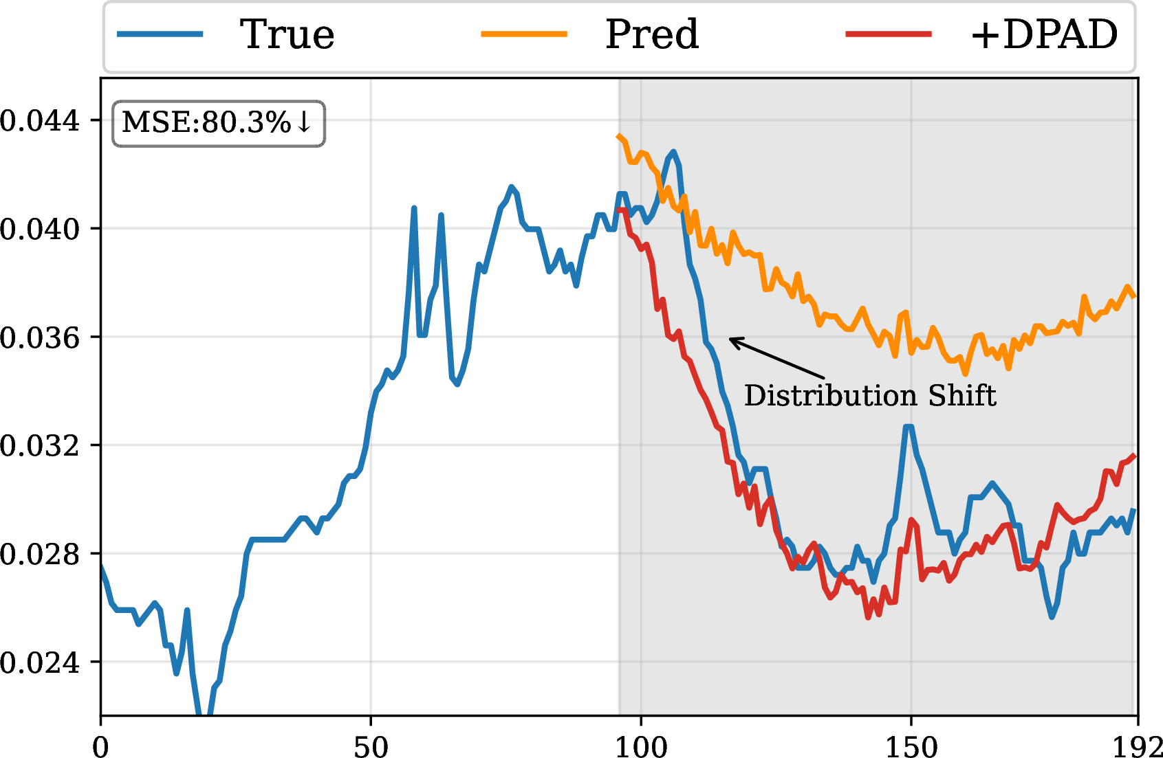
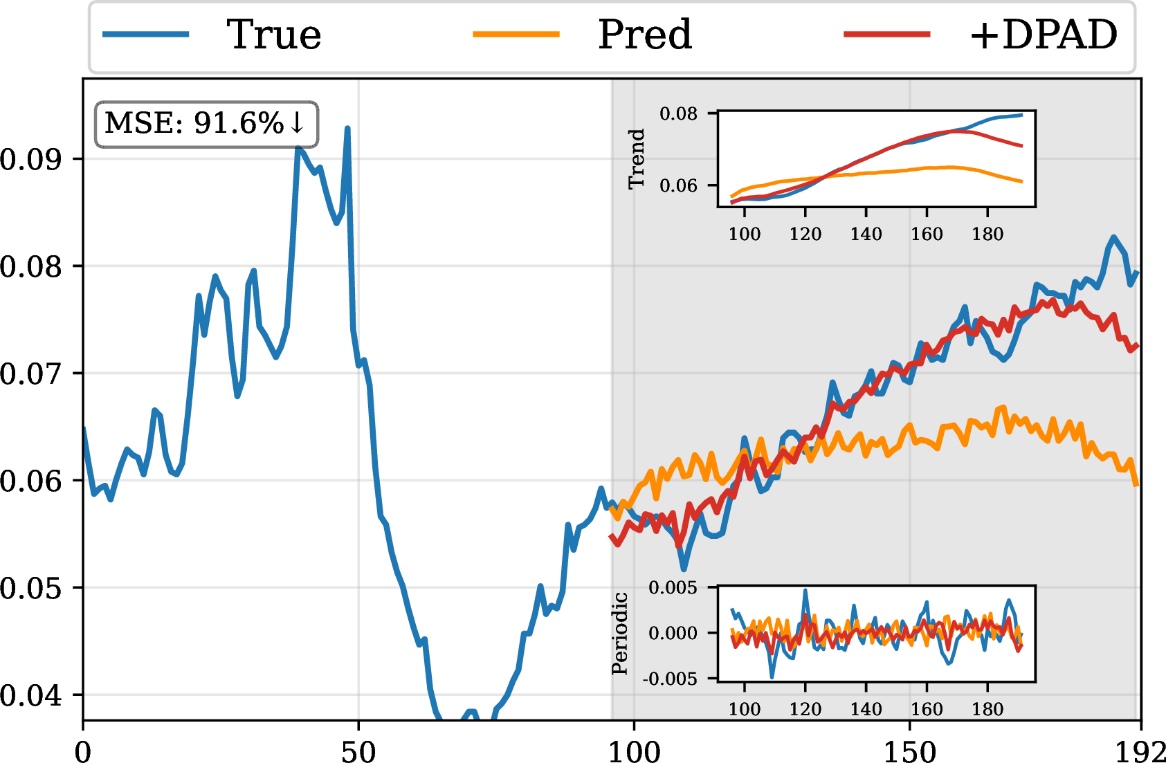
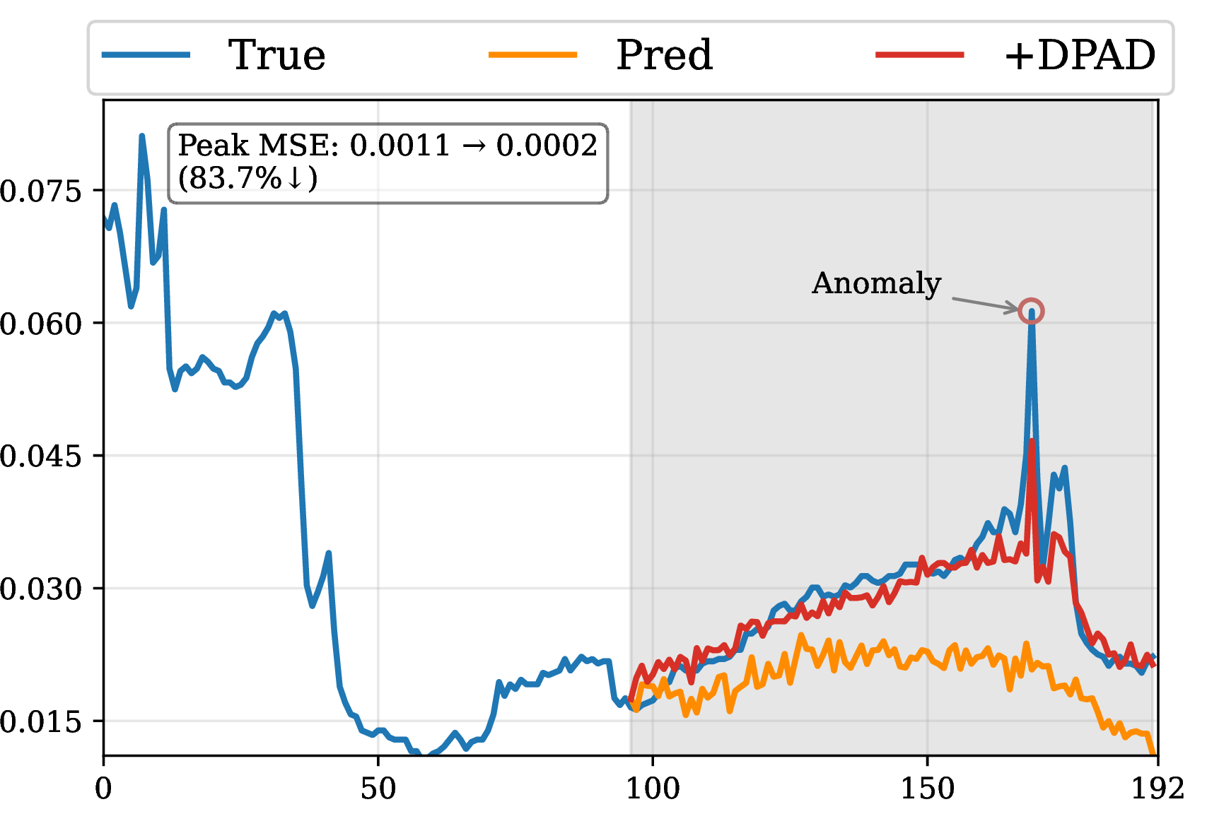
Figure 3: Case studies on failure scenarios:a) distribution shifts; b) interwined patterns; c) rare events.. a — Distribution Shifts, b — Intertwined Patterns, c — Rare Events
4.7 Model Analysis↩︎
4.7.1 Prototype Visualization.↩︎
To provide an intuitive understanding of what the DDP learns, we visualize the temporal forms of several representative prototypes from both the common and rare bank on the Weather dataset. As shown in Figure 4, the prototypes in both the common bank and rare bank evolve dynamically during training. For the common bank, the learned prototypes consistently exhibit smooth, structured shapes, including stable hybrid patterns that combine trend and seasonality components. These patterns correspond well to the intricate dependencies of the dataset, confirming that our initialization provides effective guidance and that the common bank successfully captures and refines these prevalent patterns through training. In contrast, the rare bank displays markedly different characteristics, whose prototypes are characterized by abrupt, irregular fluctuations or sudden shifts. These patterns do not conform to regular seasonal or trend patterns, which demonstrates the capability of rare set to memorize infrequent yet critical events as well as some other fluctuations.

4.7.2 Increasing Look-Back Length.↩︎
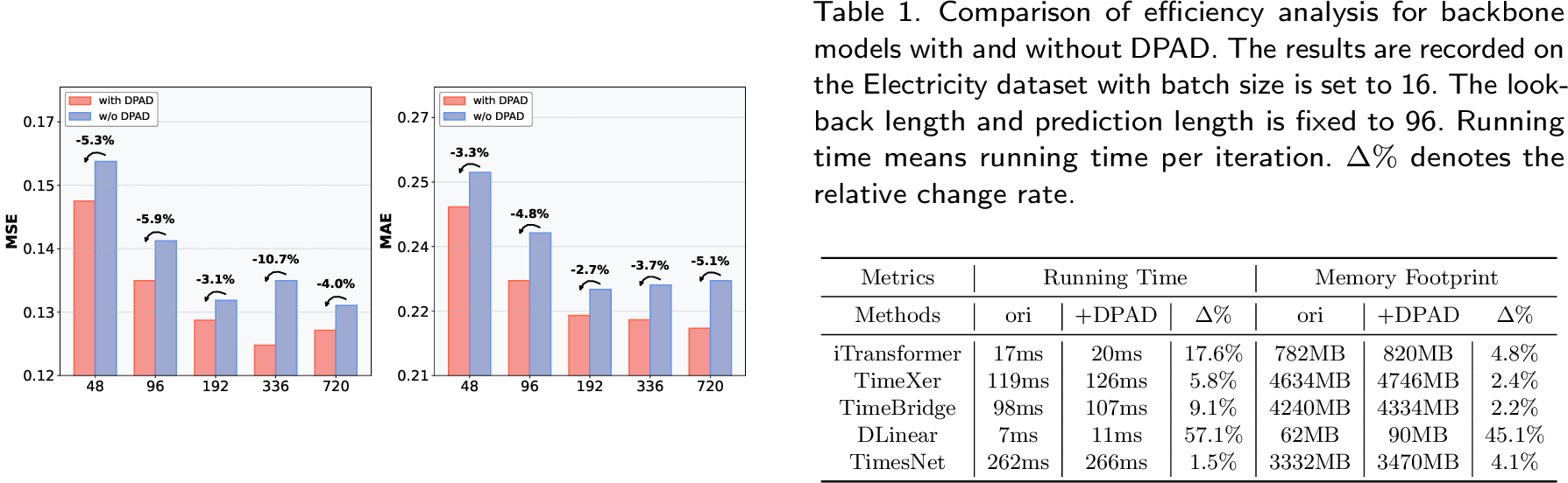
A longer look-back sequence provides richer historical information in principle, yet also presents a greater challenge due to the more complex temporal dependencies it includes. To evaluate the capability of DPAD to disentangle and leverage long-range historical context, we conduct experiments under increasing look-back length \(\{48, 96, 192, 336, 720\}\) on the Electricity dataset, taking TimeBridge as backbone model. As shown in Figure 5, DPAD consistently achieves greater performance gains over the backbone as the sequence length increases. While vanilla backbones may suffer from information overload or struggle to focus on long-term dependencies, DPAD helps them utilize the extended history information more effectively. These results indicate that components in DPAD are particularly effective at capturing, disentangling, and selectively leveraging relevant intertwined patterns from long sequences. Our framework provides a structured mechanism to deal with the expanded context.
4.7.3 Efficiency Analysis.↩︎
We conduct the efficiency analysis for the backbone model with and without DPAD. As shown in Table [efficiency], DPAD introduces minimal overhead for most backbone models. The relative increases in running time and memory footprint are generally modest, which are below 10% for most Transformer or CNN-based backbones. While a lightweight model like DLinear shows a higher relative increase due to its extremely small base cost, the absolute added overhead remains minimal. This demonstrates DPAD is a practical and efficient enhancement module, delivering significant performance improvements while incurring only a small fraction of additional computational cost.
4.7.4 Forecasting Visualization.↩︎
To provide a more intuitive and comprehensive view of the improvements brought by our DPAD framework, we present forecasting visualizations comparing the predictions of backbone models with and without DPAD across four representative datasets. As shown in Figure 6, the predictions with DPAD are closer to the ground truth. These visualization results serve as qualitative evidence that DPAD enables more flexible, context-aware, and accurate forecasting across diverse model architectures and temporal patterns.
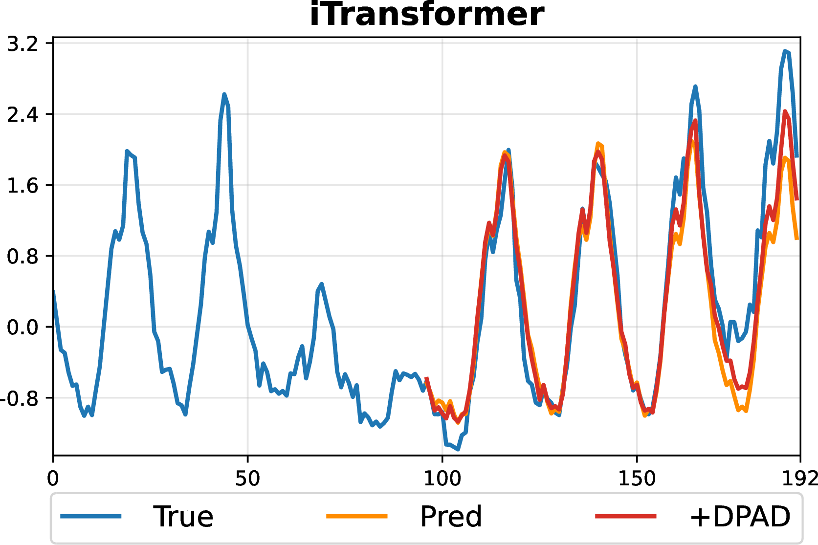


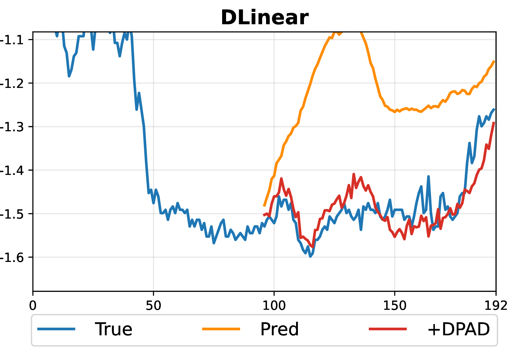

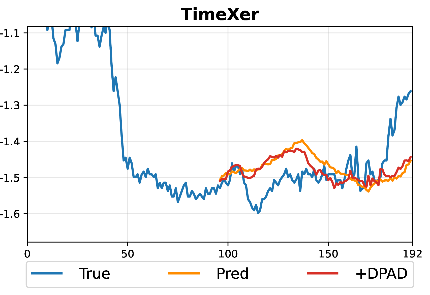
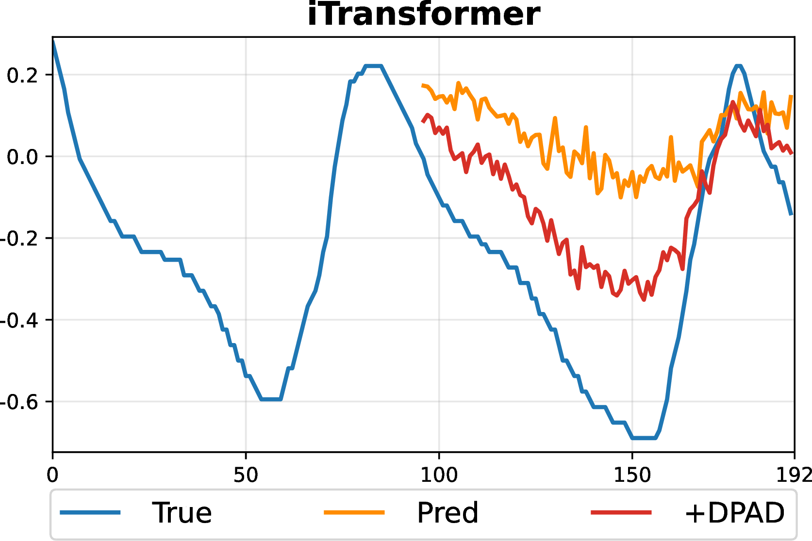
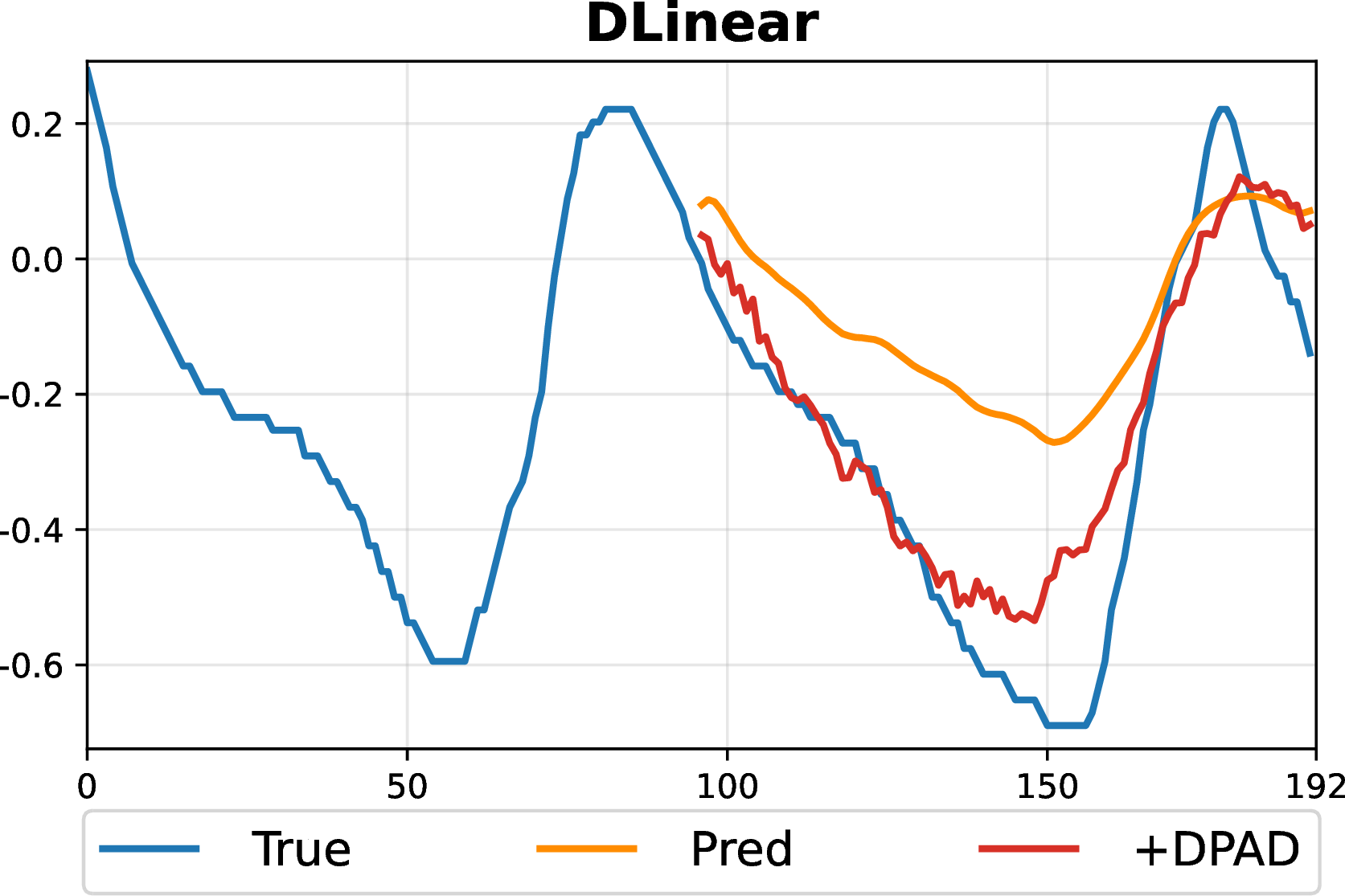
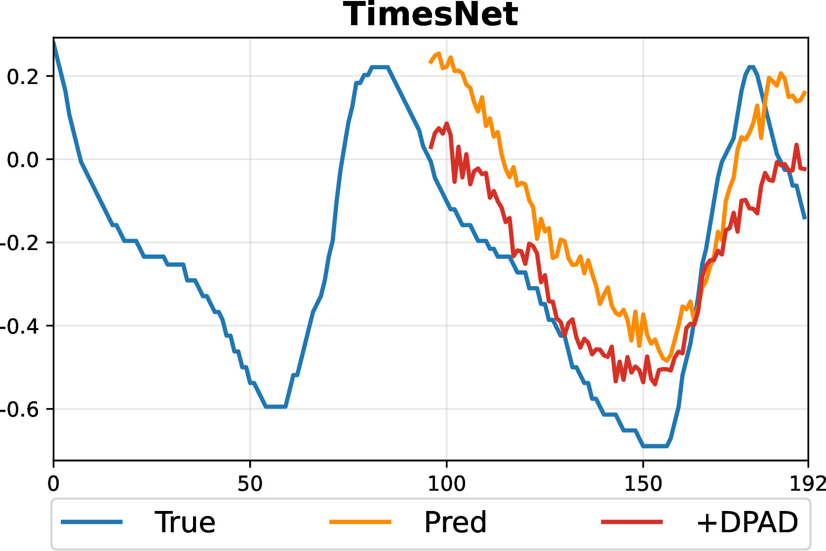
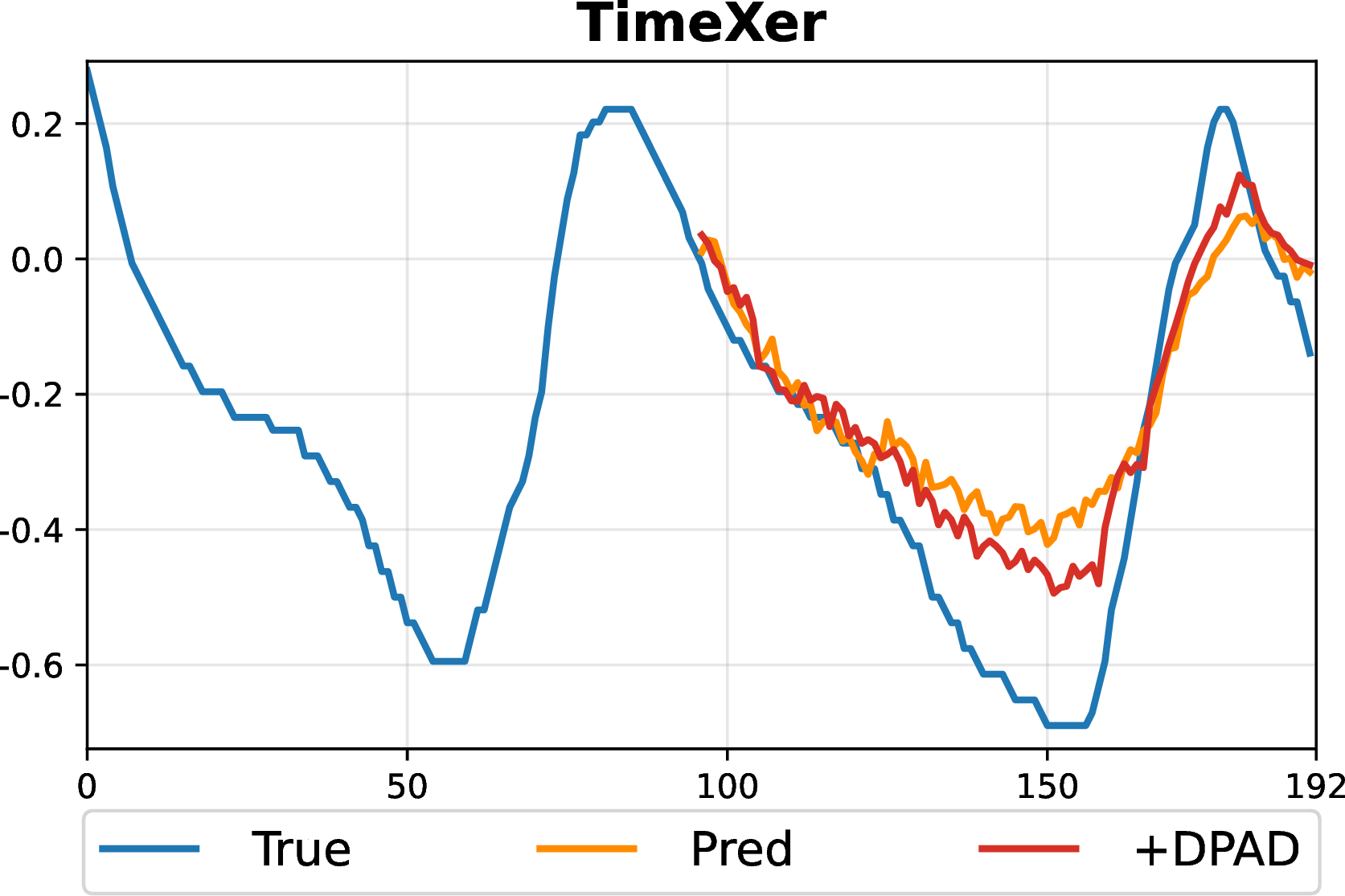
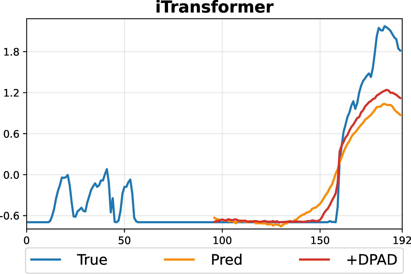
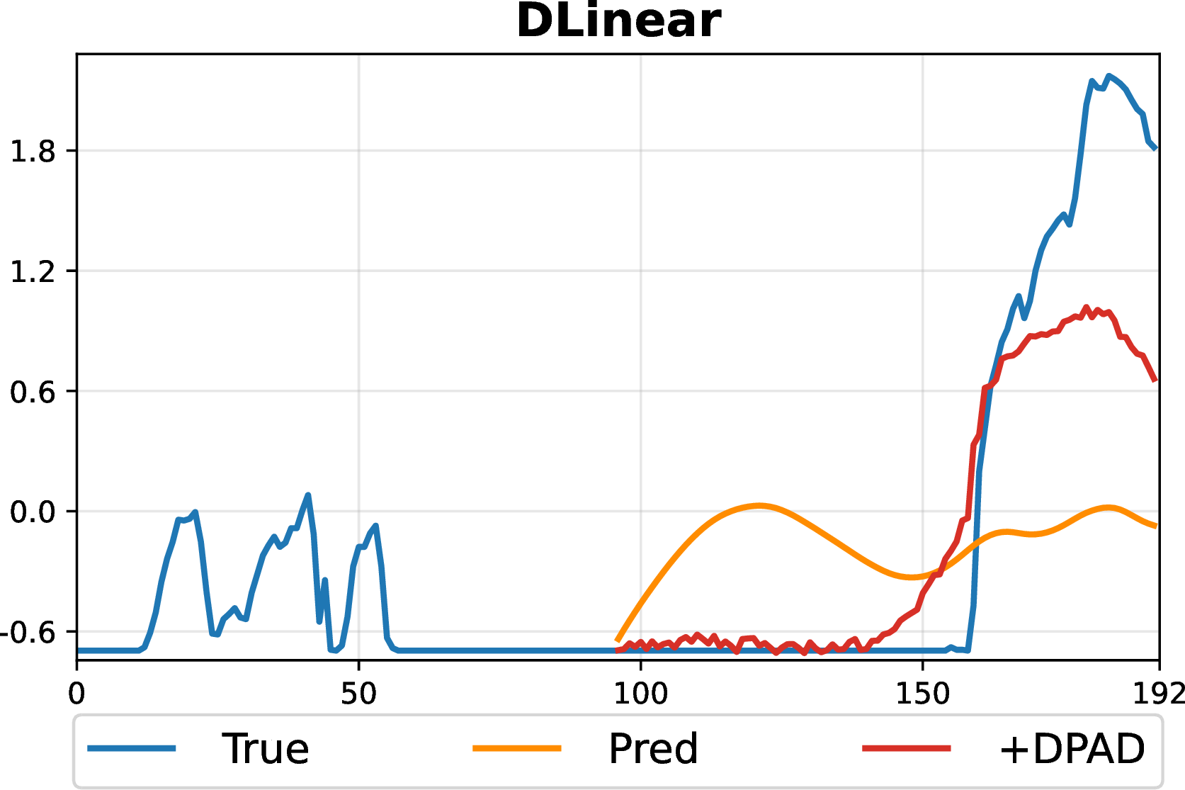
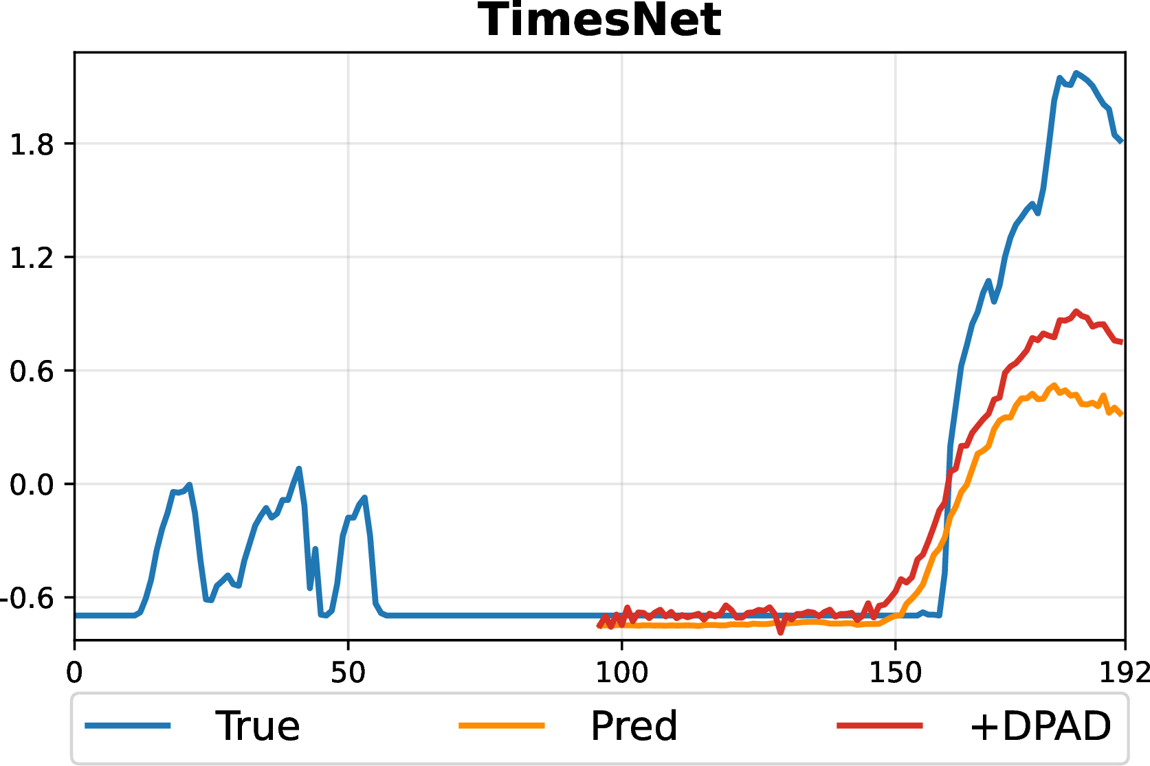
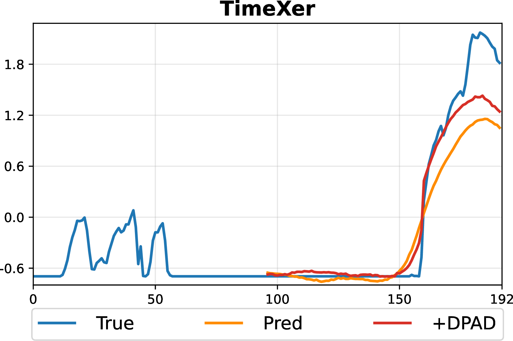
Figure 6: Forecasting visualization for backbone models with and without DPAD..
4.8 Hyperparameter Sensitivity Analysis↩︎
4.8.1 Size of Prototype Banks.↩︎
The sizes of the Common Pattern Bank \(\mathcal{B}_c\) and Rare Pattern Bank \(\mathcal{B}_r\) determine the representational capacity and specialization degree of our Dual‑Prototype Bank. To analyze their impact, we set \(\mathcal{B}_c \in \{32, 64, 128, 256\}\) and \(\mathcal{B}_r \in \{8, 12, 24, 32\}\) respectively on the Weather and ETTh2 dataset. As shown in Figure 7, the results remain stable across a broad range of sizes, indicating that DPAD is not highly sensitive to the size of prototype banks. Extremely small banks may limit the ability to capture pattern diversity, while very large banks offer no further gain and may slightly degrade performance due to increased optimization difficulty. The above observation confirms that DPAD is robust across various cases without requiring delicate tuning.
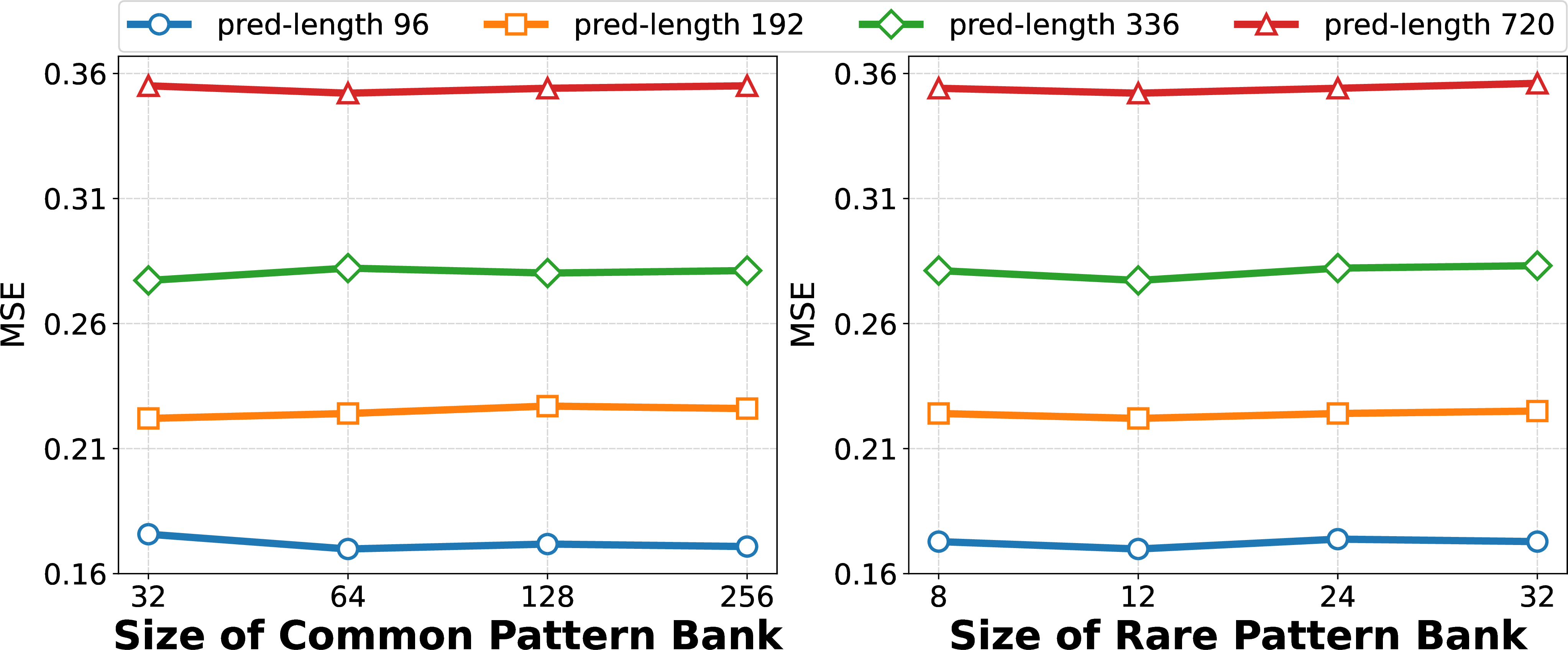
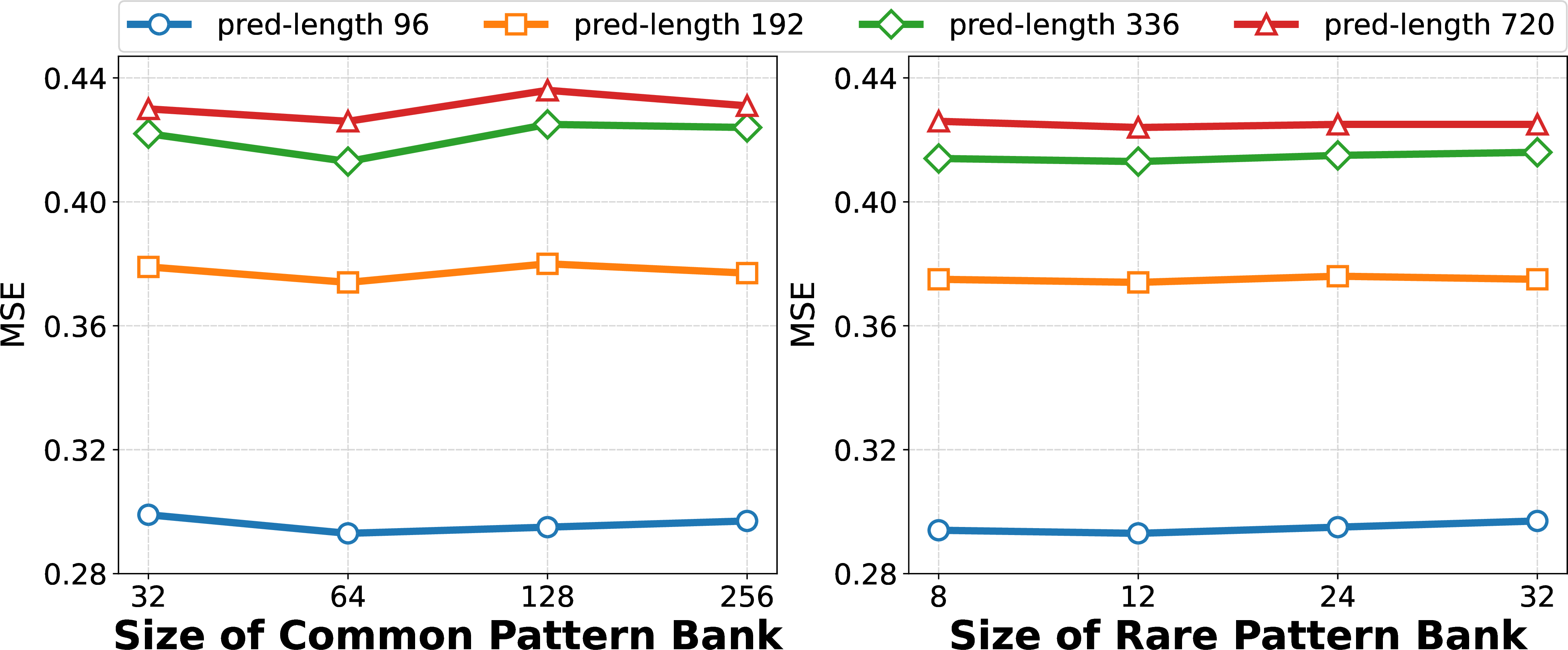
Figure 7: Hyperparameter sensitivity analysis with varying sizes of prototype banks on Weather dataset. Here we use iTransformer as backbone. Left is of common pattern set, right is of rare patterns set. The look-back length is fixed to 96.. a — On Weather dataset., b — On ETTh2 dataset.
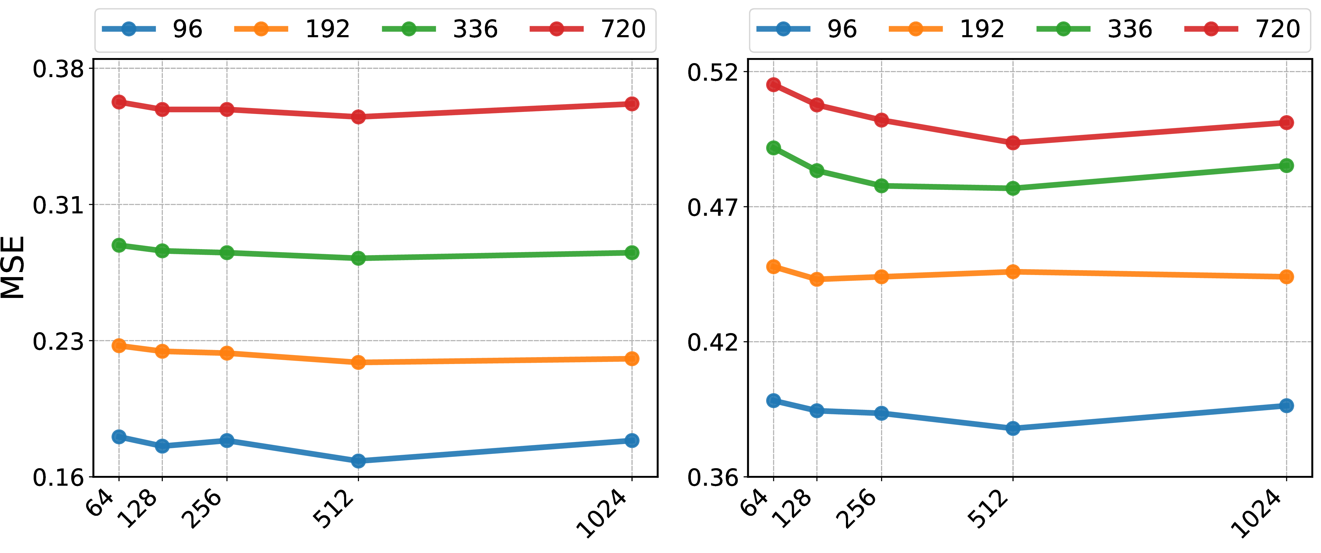
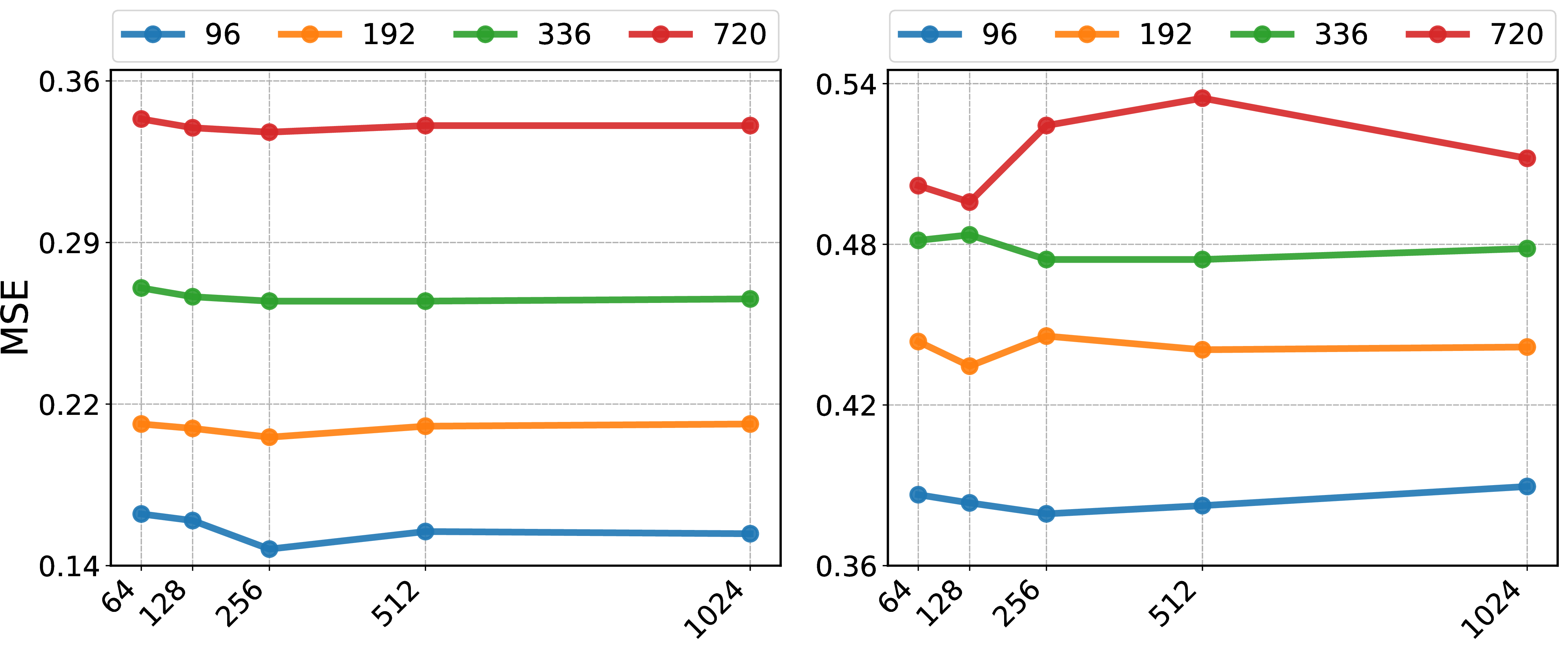
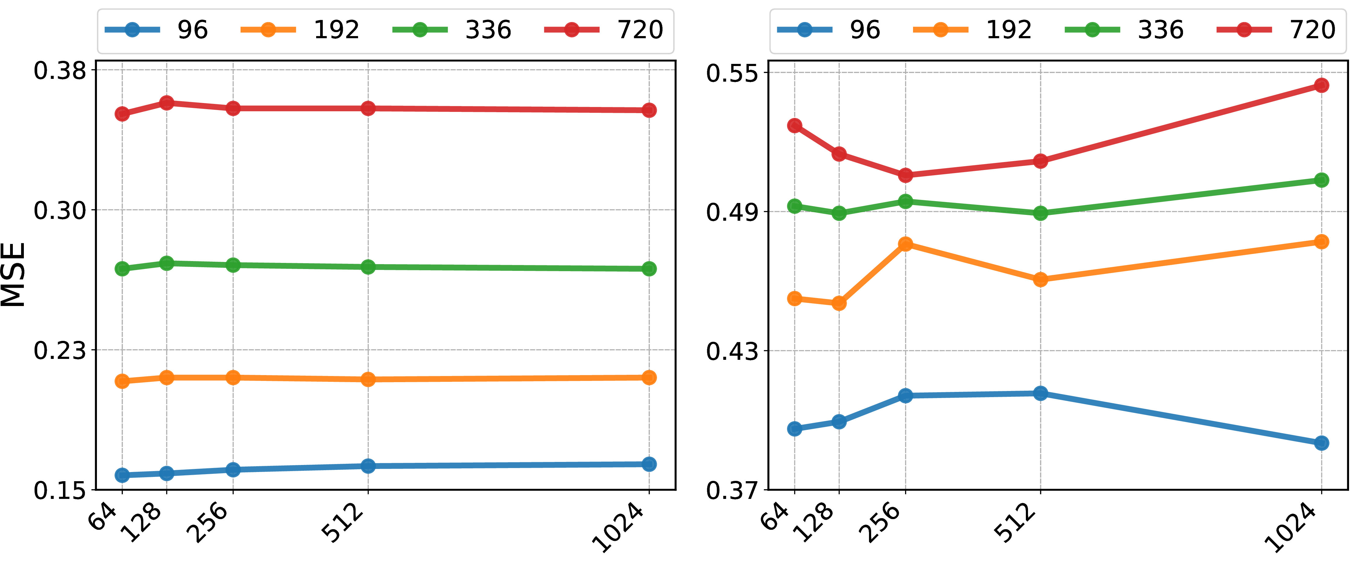
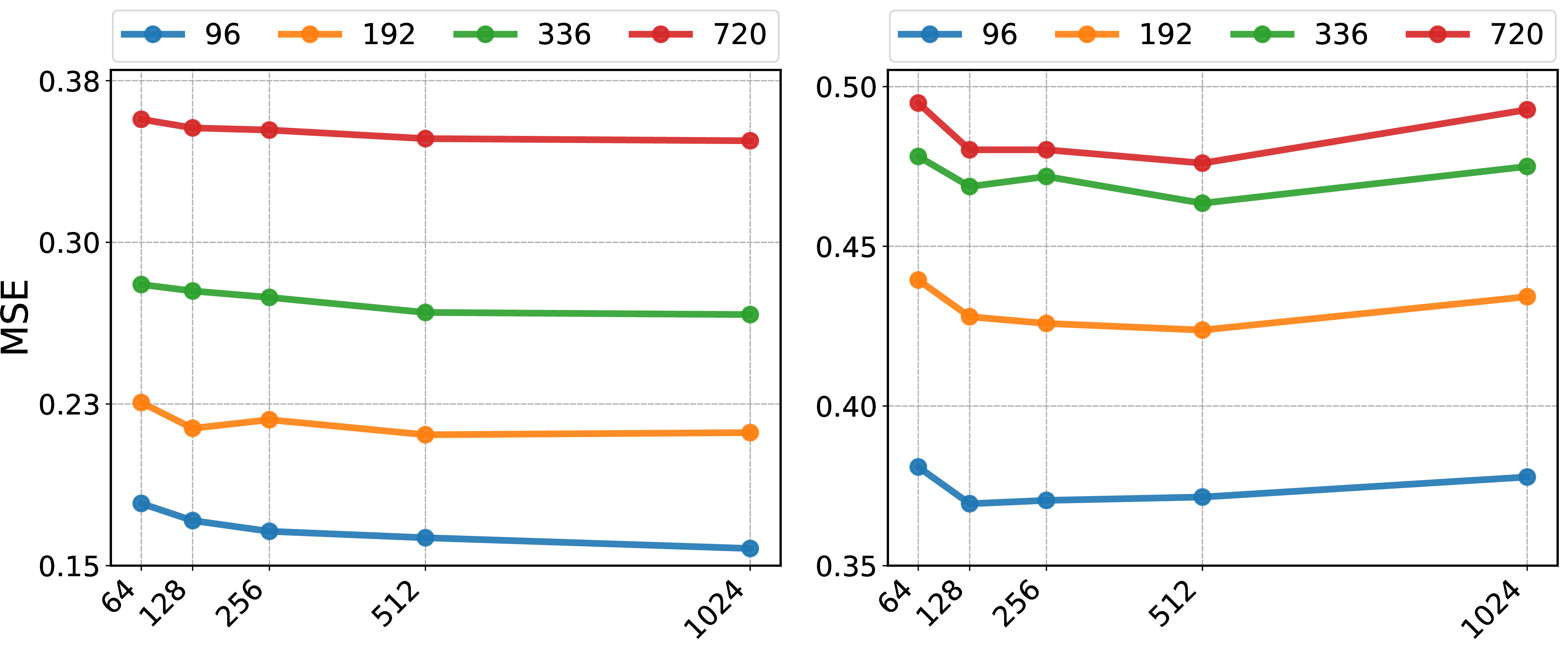
Figure 8: Hyperparameter sensitivity analysis on embedding dimension. For each backbone, forecasting results are on the Weather (left) and ETTh1 (right) datasets. The look-back length length is fixed to 96.. a — With iTransformer as backbone., b — With TimeXer as backbone., c — With TimesNet as backbone., d — With TimeBridge as backbone.
4.8.2 Embedding Dimension.↩︎
The embedding dimension determines the richness of feature representations in the unified projection space. We vary \(d_{\text{model}} \in \{64, 128, 256, 512, 1024\}\) on the Weather and ETTh1 dataset with four backbone models to evaluate its impact. As shown in Figure 8, in most cases DPAD exhibits low sensitivity to the choice of embedding dimension. Performance does not degrade significantly even at relatively small dimensions, while larger dimensions provide only marginal gains. So we choose the optimal dimension at 128/256 in most cases. The above observation indicates that our dual-prototype architecture and routing mechanism are effective at capturing and utilizing pattern information without requiring a high-dimension latent space. This property further simplifies the deployment of DPAD as a plug-and-play module.
4.8.3 Weights of DGLoss.↩︎
The weight \(\lambda_\text{sep}, \lambda_\text{rare}, \lambda_\text{div}\) of the DGLoss controls the strength of separation, rarity preservation, and diversity of temporal prototypes. To analyze their individual effects, we vary them in \(0.001 - 2.0\) on electricity and weather datasets. As shown in Figure 9, the forecasting performance remains stable across a wdie range of weight values. Specifically, the MSE exhibit only minor fluctuations when the weights are varied from \(0.001 - 2.0\), indicating that the proposed DGLoss is not highly sensitive to the exact choice of these hyperparameters, which simplifies the deployment of DPAD in practice.
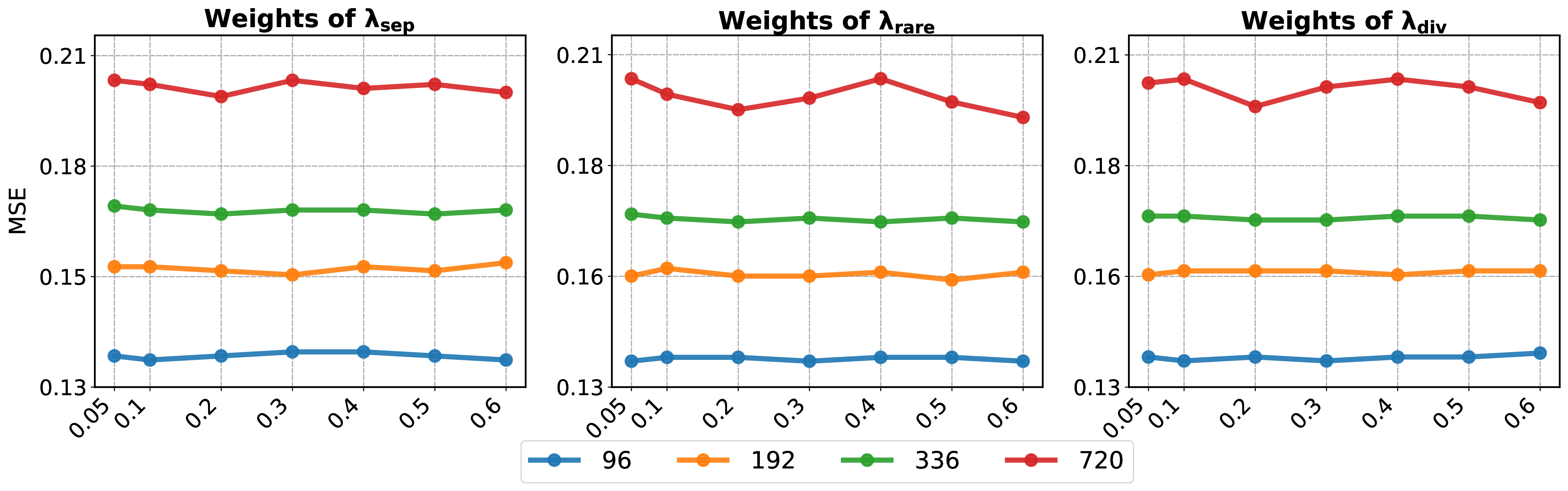
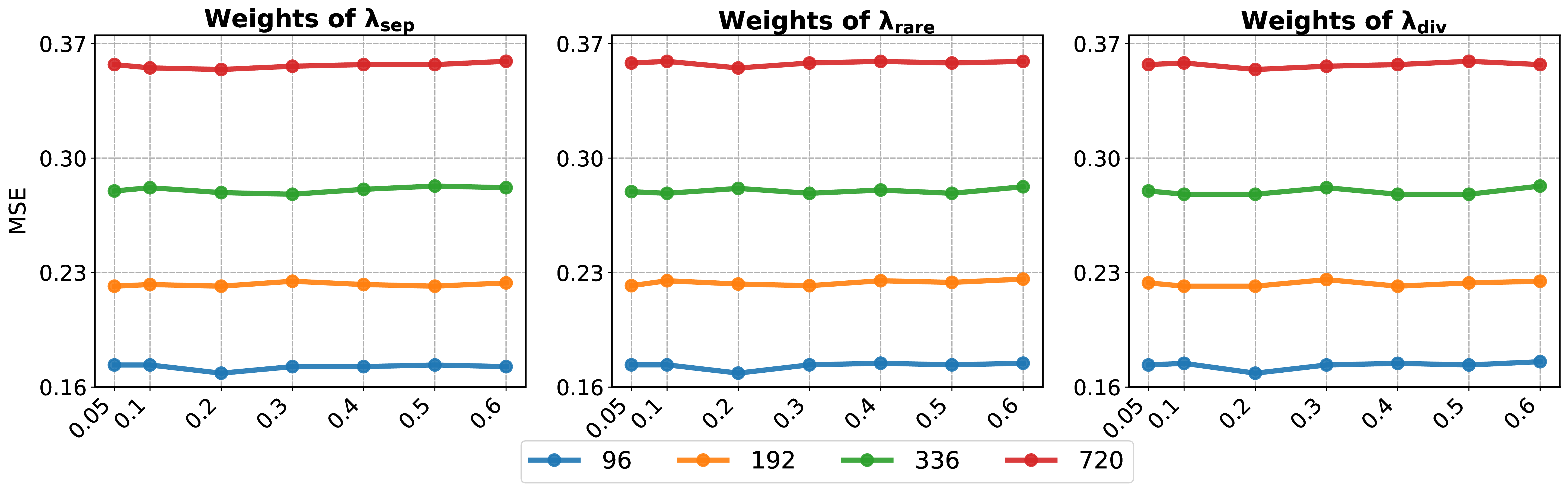
Figure 9: Hyperparameter sensitivity analysis on weights of DGLoss. Forecasting results are on the ECL and Weather datasets, and we use TimeBridge as backbone model. The look-back length length is fixed to 96.. a — On ECL dataset., b — On Weather dataset.
5 Conclusion↩︎
In this paper, we address a critical limitation of static and averaged representations in deep time series forecasting, which hinders model adaptability to intricate and dynamic contexts. We propose the Dual-Prototype Adaptive Disentanglement (DPAD) framework, a model-agnostic auxiliary method that enhances the backbone model through a Dynamic Dual-Prototype bank (DDP), Dual-Path Context-aware routing (DPC), and a Disentanglement-Guided Loss (DGLoss). Extensive experiments validate that DPAD consistently improves forecasting performance while introduces minimal computational overhead. Future work may explore more interpretable routing mechanisms and a novel prototype paradigm with multi-modal representations.