Non-Ambipolarity of Microturbulent Transport
January 22, 2026
Abstract
When restricted to magnetic flux tubes, the gyrokinetic theory of microturbulence gives the same radial transport for ions and electrons. But, exact magnetic surfaces do not exist in the presence of what is called electrostatic microturbulence. At a finite plasma pressure, a turbulent electric potential is accompanied by a turbulent magnetic field \(\tilde{B}\), which makes the magnetic field lines chaotic. Quasi-neutrality along the chaotic magnetic field lines requires a potential that obeys \(en \color{black} \vec{B}\cdot \vec{\nabla} \Phi = \vec{B}\cdot \vec{\nabla} p_e\), where \(p_e\) is the electron pressure. This potential produces radial transport similar to that of diffusion coefficient \(D_{ef}= (\Delta/a_T)T_e/eB\). \(\Delta\) is the radial distance over which the potential \(\Phi\) is correlated by the electron motion along the chaotic magnetic field, and \(|dT_e/dr| = T_e/a_T\). The chaos-produced electron transport gives an effective viscosity on the electron flow, which can counterbalance a non-ambipolar part of the ion radial particle diffusion that is \(f_{na}\) times gyro-Bohm diffusion. This non-ambipolarity would otherwise require a radial electric field that confines ions and hence impurities. The maximum \(f_{na}\) that can be counterbalanced and the required plasma beta to avoid shielding the magnetic perturbations \(\tilde{B}\) are calculated.
1 Introduction↩︎
Nevins, Wang, and Candy [1], Connor, Hastie, and Zocco [2], and Terry et al [3] have discussed magnetic surface breakup produced by what are called electrostatic instabilities, primarily the ion temperature gradient (ITG) instability. The focus has been on the enhancement of the electron heat transport, which is not large when the plasma \(\beta\equiv 2\mu_0p/B^2\) is small.
An effect that can arise before the electron heat transport is appreciable is a modification of the radial electric field required to preserve quasi-neutrality in stellarators. This modification could be of great practical importance because neoclassical transport in stellarators usually gives more rapid ion than electron transport, which requires an electric field that confines ions—particularly high charge state impurities. A large expulsion of impurities in W7-X experiments was found [4] when the microturbulent transport exceeded the expected neoclassical, which requires an explanation.
Helander and Simakov [5] discussed the lack of effect of electrostatic microturbulence on the large scale radial electric field. The turbulent Reynolds stress can produce short-scale zonal flows that tend reduce the microturbulent transport. They did not discuss the effect on electron transport of the breaking of the magnetic surfaces by the turbulence. Their arguments imply the non-ambipolar radial transport of the ions is entirely due to neoclassical, not turbulent, transport effects. Sugama et al [6] included the effect of magnetic fluctuations and found microturbulence remained intrinsically ambipolar, but they assumed the magnetic surfaces were preserved.
The enhanced radial transport of electrons by turbulence modifies the radial electric field, which implies momentum transport. Unlike symmetry breaking by an external magnetic field, in which momentum changes are balanced by forces on the coils, non-ambipolarity produced by internal plasma turbulence must be due a viscosity-like force. When the radial scale of the turbulence is small, the form of this force on the electron velocity is \[\begin{align} && \vec{F}_v \equiv - \vec{\nabla}\times(\nu\vec{\nabla}\times\vec{v}_e),which satisfies \\ && \int \vec{F}_v d^3x = \oint (\nu\vec{\nabla}\times\vec{v}_e) \times d\vec{a}. \end{align}\] The force exerted throughout a volume is transmitted to the bounding surface with \(\nu(\vec{x},t)\) an effective viscosity coefficient.
To simplify the statement of results, the fraction of the radial ion transport that is non-ambipolar, \(f_{na}\) is defined relative to the typical gyro-Bohm radial transport. In optimized stellarators, the gyro-Bohm radial transport due to microturbulence is large compared to the neoclassical radial transport, which implies \(f_{na}\) is small compared to unity.
2 Perturbed magnetic field due to microturbulence↩︎
The effect of microturbulence on the magnetic field is easier to understand when the velocity of the magnetic field lines \(\vec{u}_\bot\) is distinguished from the mass-flow velocity \(\vec{v}\) of the plasma. The field-line velocity can be defined using the representation of an arbitrary vector \(\vec{E}\) in terms of another arbitrary vector \(\vec{B}\), Equation (26) in [7], \[\vec{E}+\vec{u}_\bot \times \vec{B} = - \vec{\nabla}\Phi + V_\ell \vec{\nabla}\frac{\varphi}{2\pi}, \label{E-exp}\tag{1}\] which is a mathematical identity. This equation can be inserted into Faraday’s Law to obtain an equation with general validity, \[\begin{align} \frac{\partial \vec{B}}{\partial t} = \vec{\nabla} \times (\vec{u}_\bot \times \vec{B}) + \frac{\vec{\nabla}V_\ell \times \vec{\nabla}\varphi }{2\pi}. \label{Ad-diff} \end{align}\tag{2}\] When the term \((\vec{\nabla}V_\ell \times \vec{\nabla}\varphi)/2\pi\) involves second derivatives of \(\vec{B}\) with respect to position then it is diffusive. This is the case when there is a term \(\eta\vec{j}\) in the expression for the electric field, which diffuses magnetic field lines with \(\eta/\mu_0\) the diffusion coefficient. Equation (2 ) is then an advection-diffusion equation.
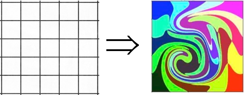
Figure 1: A magnetic field \(\vec{B}(\vec{x},t)\) can be thought of as consisting of tubes of magnetic flux by placing a gridded surface across the field. Each tube is defined by the magnetic field lines that pass through the perimeters of the grid cells. When the field is chaotic, the perimeter of each cell becomes exponentially longer when the grid is replotted after each line on the perimeters is followed for a distance \(\ell\). But, each cell contains exactly the same field lines and has precisely the same neighboring cells. When the magnetic field is evolving ideally with a chaotic velocity \(\vec{u}_\bot\), a similar distortion of the grid occurs when the grid is replotted using the location of each line on the perimeters after a time \(t\). The figure shows the distortion of a \(5\times5\) array. This is Figure 1 of Boozer, Phys. Plasmas 32, 052106 (2025). The distorted grid is part of Figure 5 of Y.-M. Huang and A. Bhattacharjee, Phys. Plasmas 29, 122902 (2022), which was based on a chaotic evolution defined by A. H. Boozer and T. Elder, Phys. Plasmas 28, 062303 (2021). Boozer and Elder illustrated distortions of ideally evolving flux tubes up to a factor \(\sim 10^7\)..
A magnetic field line flow \(\vec{u}_\bot\) driven by turbulence is chaotic, which means neighboring streamlines of the flow separate exponentially in time with timescale \(\tau_u\). What many find surprising is that magnetic surfaces will break on a timescale only an order of magnitude longer than \(\tau_u\) no matter how small the resistive diffusion \(\eta/\mu_0\) may be. Resistivity enters the reconnection timescale only logarithmically [8], [9]. Figure 1 illustrates how chaos exponentially enhances the effect of \(\eta/\mu_0\) diffusion on reconnection.
Although chaotic flows can rapidly break magnetic surfaces, the timescale for the re-formation of magnetic surfaces is not shortened by a chaotic flow. A resistive timescale is required—not the logarithm of the resistive timescale as in the breaking. This lack of time reversibility in mixing is well known in everyday life. Ingredients in soup are mixed by stirring, but they cannot then be separated by stirring in the opposite direction. The time-reversibility of solutions to an advection-diffusion equation is exponentially sensitive to the diffusion.
A slab-model, in which a constant magnetic field \(B_z\hat{z}\) is subjected to a perturbation \(\tilde{B}_x\hat{x}\), illustrates the relationship between the magnetic field line velocity \(\tilde{u}_x\hat{x}\) and the plasma velocity \(\tilde{v}_x\hat{x} + \tilde{v}_z\hat{z}\). Equation (2 ), with an ideal perturbation, \(\vec{\nabla}V_\ell=0\), implies \(\partial_t \tilde{B}_x = B_z\partial_z \tilde{u}_x\), so \(\partial_z \partial_t \tilde{B}_x = B_z\partial_z^2 \tilde{u}_x\). Ampere’s Law implies \(\partial_z \tilde{B}_x = \mu_0 j_y\) and force balance gives \(j_y B_z = m_i n \partial_t \tilde{v}_x\), which leads to the equation \(\partial_z \partial_t \tilde{B}_x = \frac{\mu_0 m_i n}{B_z} \partial_t^2 \tilde{v}_x.\) Equating the two expressions for \(\partial_z \partial_t \tilde{B}_x\), \[\begin{align} \frac{\partial^2 \tilde{u}_x}{\partial z^2} &=& \frac{\mu_0 m_i n}{B_z^2} \frac{\partial^2 \tilde{v}_x}{\partial t^2}\\ &=& \frac{1}{V_A^2} \frac{\partial^2 \tilde{v}_x}{\partial t^2}. \end{align}\] When the phase velocity of \(\tilde{v}_x\) along \(z\) equals the Alfvén speed, \(\tilde{u}_x=\tilde{v}_x\), and the whole motion of the plasma is due to the motion of the magnetic field lines, which means an Alfvén wave. When the phase velocity along \(z\) is approximately the the speed of sound \(C_s=\sqrt{T/m_i}\), then \(\tilde{u}_x = (C_s^2/V_A^2)\tilde{v}_x\). The ratio \(C_s^2/V_A^2 \sim \beta\), and the magnetic field lines move little compared to the plasma motion. Nevertheless, the velocity of the magnetic field lines is turbulent and, therefore, chaotic, which implies magnetic reconnection that breaks the magnetic surfaces will quickly occur [8], regardless of how small non-ideal effects represented by the loop voltage may be.
When potential fluctuations \(\tilde{\Phi}\) have a phase velocity along the field lines \(\approx C_s\), there is cross magnetic surface magnetic fluctuation \[\begin{align} \frac{\tilde{B}}{B} &\approx& \left(\frac{C_s}{V_A}\right)^2 \frac{e\tilde{\Phi}}{T} \\ & \approx& \beta \frac{ e\tilde{\Phi}}{T }. \label{Phi-fluc} \end{align}\tag{3}\]
Even an ideally but turbulently fluctuating \(\vec{\tilde{B}}\cdot\vec{\nabla}\psi_t\):
Creates delta-function currents at resonant rational surfaces [10] , which quickly form islands. Different island chains exert phase dependent forces depending on their relative phase and will lock together at sufficient magnitude.
Causes the distortion of flux tubes [8], [9], which allows an arbitrarily small \(\eta/\mu_0\) to mix lines from different tubes, Figure 1. Once magnetic surfaces are broken, they do not easily heal. Surface breaking will persist as long as the turbulence does.
3 Effect on Electrons↩︎
When the magnetic field chaos is on a large scale compared to the electron gyroradius, electrons move rapidly along \(\vec{B}\). To maintain quasi-neutrality when there is an electron pressure gradient along a magnetic field line, the electric potential must satisfy \(\color{black}en\color{black}\vec{B}\cdot \vec{\nabla} \Phi = \vec{B}\cdot \vec{\nabla} p_e\). The \(\Phi\) required for quasi-neutrality is \(\sim T_e/e\). In a chaotic magnetic field, the variation across the field lines in the electric potential required for quasi-neutrality gives complicated \(\vec{E}\times \vec{B}\) plasma flows and a radial transport comparable to an effective diffusion coefficient \(D_{ef}\) [11]. Let \(\Delta\) be the radial correlation distance of the quasi-neutrality electric potential along the chaotic magnetic field lines, then the potential variation from one line of \(\vec{B}\) in a pressure surface to another is \(\sim (\Delta/a_T) (T_e/e)\), where \(|dT_e/dr| = T_e/a_T\). The correlation distance in a pressure surface is \(\sim\rho_s\), which gives a typical \(\vec{E}\times\vec{B}\) speed of \(v_{EB} \sim (\Delta/a_T)C_s\) and smooths temperature variations in the pressure surfaces on a timescale \(\rho_s/v_{EB}\). This timescale is similar to that of a diffusion coefficient \[\begin{align} D_{ef} &=& \frac{\Delta}{a_T}\frac{T_e}{eB}. \end{align}\]
Since the radial motion of the electrons changes the radial electric field and thereby the \(\vec{E}\times\vec{B}\) flow of the the ions. The implication is that \[\nu = m_i n D_{ef} \color{black}.\] However, the magnetic field due to turbulence may not be sufficiently stiff to reach this transport level. When it is not \(\tilde{B}\) is removed by shielding. This shielding constraint is discussed in Section 5 and found to be \(\beta\gtrsim(\Delta/ a_T) f_{na}\), Equation (6 ).
The magnitude of \(\Delta\) is the major subtlety. When followed far enough, an arbitrarily chosen field line can cover the entire region of surfaces broken through the effect of the electrostatic turbulence. Although the precise field line trajectories are changing on a timescale set by the turbulence, this has little effect on the probability a magnetic field line will have a large change in its radial position over a certain distance. When both \(\beta<<1\) and \(f_{na}\) are assumed sufficiently small that shielding described in Section 5 does not occur, the magnetic field as modified by the turbulence is calculable, and the magnitude of \(\Delta\) could be studied. A plausible assumption is that \(\Delta/\rho_s \sim (\tilde{B}/B)( v_{th}^e/v_{EB})\) with \(v_{th}^e\) the electron thermal speed. Since \(\tilde{B}/B \sim \beta \rho_s/a,\) this would imply \(\Delta/\rho_s \sim \sqrt{\beta \sqrt{m_i/m_e}}\) or \(\Delta\sim \rho_s\).
The momentum conserving force balance equations for electrons and ions are \[\begin{align} m_en \frac{d\vec{v_e}}{dt} &=&- en (\vec{E} + \vec{v}_e \times \vec{B}) -\vec{\nabla}p_e + \vec{F}_v; \\ m_in \frac{d\vec{v}}{dt} &=& en (\vec{E} + \vec{v} \times \vec{B}) -\vec{\nabla}p_i + \vec{F}_{na}, \end{align}\] where the mass-flow speed is identified with the ion velocity. The ions have an intrinsic non-ambipolar drag force which will be derived below in the approximation of circular magnetic surfaces.
Since \(\vec{j}=en(\vec{v} - \vec{v}_e)\), when the the electrons are assumed to be massless, the sum of the two force-balance equations is \[\begin{align} m_i n \frac{d\vec{v}}{dt} = \vec{j}\times\vec{B} - \vec{\nabla}p + \vec{F}_{na} + \vec{F}_v. \label{fluid-force} \end{align}\tag{4}\]
4 Near-circular surface approximation↩︎
When the magnetic surfaces are nearly circular, \((r,\theta,\varphi)\) orthogonal coordinates can be used, which are \((r,\theta,z)\) cylindrical coordinates with \(\varphi \equiv z/R\). The \(z\) coordinate is periodic with a period \(2\pi R\). The minor radius \(r\) is assumed to be very small compared to the major radius \(R\). The flows associated with equilibrium balance are in the \(\hat{\theta}\equiv r \vec{\nabla}\theta\) direction.
Equilibrium force balance occurs on a fast timescale compared to rotation changes and requires \(\vec{j}\times\vec{B} = \vec{\nabla}p(r)\). The implication is that \(en(v-v_e)\hat{\theta}\times B_\varphi \hat{\varphi} = (dp/dr) \hat{r}\). The ion and electron flows are in the \(\hat{\theta}\) direction and obey \[\begin{align} v&=& v_e + v_p\\ v_p &\equiv& \frac{dp/dr}{en B_\varphi}\\ |v_p|&\approx& \frac{T}{aeB_\varphi}\\ &\approx& \frac{\rho_s }{a} C_s \end{align}\] where \(v_p\) is assumed to be a constant in time, \(C_s = \sqrt{T/m_i}\), and \(\rho_s = C_s/(eB_\varphi/m_i)\).
The ions intrinsic non-ambipolar drag force is \[\begin{align} \vec{F}_{na} &=& j_r \hat{r} \times B_\varphi\hat{\varphi} \\ &=&- j_rB_{\varphi}\hat{\theta}.\\ | j_r| &=& en \frac{a}{\tau_p^{na}} \left| \frac{v}{v_p}\right| \end{align}\] The non-ambipolar particle confinement time \(\tau_p^{na}= a^2 / f_{na} D_{gb}\), where \(D_{gb}\equiv (\rho_s/a)(T/eB)\) is a typical transport coefficient, \(f_{na}\) is the dimensionless relative strength of the non-ambipolar transport compared to the total transport, and \(B=B_{\varphi}\). Then \[\begin{align} \vec{F}_{na} &=& - en \frac{a}{\tau_p^{na}} \frac{v}{|v_p|} B_\varphi \hat{\theta}\\ &=& - en \frac{f_{na}D_{gb}}{a} \frac{v}{(\rho_s/a) C_s} B_\varphi \hat{\theta}\\ &=& - f_{na} \frac{m_i n D_{gb}}{\rho_s^2} v \hat{\theta}. \end{align}\]
The steady-state solution to Equation (4 ) is \((\vec{F}_{na} + \vec{F}_v)\cdot\hat{\theta}=0\) with the radial component giving \(v= v_e + v_p\), \[\begin{align} \left| f_{na} \frac{m_i n D_{gb}}{\rho_s^2} v \right| &=& \left| \vec{\nabla}\times(\nu\vec{\nabla}\times\vec{v}_e)\right|\\ &\approx& \left| \nu \frac{d}{dr}\Big(\frac{1}{r} \frac{d rv_e}{dr}\Big)\right|\\ &\approx& \nu \frac{\left|v_e\right|}{a^2} \\ \left| \frac{v_e}{v}\right| &\approx& \frac{f_{na} \frac{m_i n D_{gb}}{\rho_s^2}}{\nu /a^2}\\ &\approx& f_{na} \left(\frac{a}{\rho_s}\right)^2 \frac{D_{gb}}{D_{ef}}\\ &\approx& f_{na} \left(\frac{a}{\rho_s}\right) \frac{ a_T}{\Delta} \label{v95e47v}, \end{align}\tag{5}\] since \(\nu= m_in D_{ef}\). To change the electric field, \(|v_e/v| \lesssim1\) is required, or \[f_{na} \lesssim \frac{\rho_s}{a}\frac{\Delta}{a_t}.\] When the right-hand side Equation (5 ) is large, \(|v|\rightarrow0\), and the electrons provide the confinement
5 Shielding constraint↩︎
Force in the \(\hat{\theta}\) direction exerted by magnetic perturbation is \(k_\theta \tilde{B}^2/\mu_0\), where \(1/k_\theta \approx \rho_s\) is the distance scale of \(\tilde{B}\) variations in the poloidal direction. This magnetic force must be strong enough to balance \(\vec{F}_{na}\cdot\hat{\theta}\) to make the ion flow provide the confinement. \[\begin{align} \frac{\tilde{B}^2}{\mu_0} &>& \left| \frac{\vec{F}_{na}\cdot\hat{\theta}}{k_\theta} \right|\\ &>& f_{na} \frac{m_i n D_{gb}}{\rho_s^2} \frac{|v_p|}{k_\theta} \\ &>& f_{na} \frac{m_i n }{\rho_s^2} \left(\frac{\rho_s}{a} \frac{T}{eB} \right) \Big(\frac{\rho_s}{a} C_s \Big)\frac{1}{k_\theta}\\ &>& \frac{f_{na}}{k_\theta a} \frac{\rho_s}{a} \beta \frac{B^2}{\mu_0}\\ \frac{\tilde{B}^2}{B^2} &>& \frac{\beta f_{na}}{k_\theta a} \frac{\rho_s}{a},or using Eq. (\ref{Phi-fluc}) \\ \Big(\frac{a}{\rho_s} \frac{e\tilde{\Phi} }{T}\Big)^2 &>&\color{black} \frac{f_{na}}{\beta}\frac{\Delta}{a_T}. \end{align}\] with \(k_\theta\approx 1/\rho_s\). The expected amplitude of microturbulence is \(e\tilde{\Phi}/T\sim \rho_s/a\). Equation (5 ) for the ratio of \(v_e/v\) implies that shielding of \(\tilde{B}\) does not prevent the ion flow from being stopped by the microturbulence when \[\beta\color{black} \gtrsim \frac{\Delta}{a_T}f_{na}. \label{Eq:shielding}\tag{6}\]
6 Major results↩︎
There are two major results: (1) The condition for the radial electric field to pull in or to push out ions and impurities. This condition is given by the ratio of the confining current of electrons to the confining current of ions \(|env_e|/|env| \approx f_{na} (a/\rho_s) (a_T/\Delta )\), Equation (5 ). When the electron flow is large compared to the ion flow, the electrons are providing the confinement and the radial electric field pulls in the ions and impurities. The opposite is true when the electron flow is small. (2) The condition for the shielding out of the effect \(\tilde{B}\) of the microturbulence on the magnetic field. The shielding occurs when the plasma \(\beta \color{black}\lesssim (\Delta/a_T)f_{na}\), Equation (6 ), which assumes the electric potential part of the microturbulence has reached the level \(e\tilde{\Phi}/T \sim \rho_s/a\).
Acknowledgements↩︎
This work was supported in part by the U.S. Department of Energy, Office of Science under Award No. DE-AC02-09CH11466).