Interaction between cell membranes and protein inclusions in the large-deformation regime
January 21, 2026
Abstract
Biological membranes are dynamic surfaces whose shape and function are critically influenced by prins. While membrane deformations induced by prins have been extensively studied in the small-deformation regime, a variety of processes involve strong membrane deformations. We investigate the interaction between lipid membranes and prins in the ld regime, with the finite-element method. We develop an approximate analytical solution that captures key features of the ld regime. We show that the force exerted by the membrane on a prin displays non-monotonic behavior with respect to the prin vertical displacement. The qualitative features of this force appear to be independent of the protein geometry. For two interacting prins, the membrane-mediated potential exhibits sub-power-law decay with inter-protein distance, reflecting the complex nature of the elastic medium. The interaction potential shows that conical prins with identical and opposite orientations repel and attract, respectively, confirming the analogy between prin orientation and electric charge, in the ld regime. In the presence of membrane flows, we identify a characteristic velocity that separates two regimes in which bending rigidity and viscous effects dominate, respectively, implying the onset of flow-induced deformations above such velocity threshold. Overall, our results provide quantitative predictions for membrane-protein systems in biologically relevant scenarios involving lds, with implications for protein sorting, clustering, and membrane trafficking.
1 Introduction↩︎
Biological membranes are dynamic and deformable surfaces whose shape and function are critically influenced by the presence of prins [1], [2]. Such prins often impose geometric constraints, e.g., contact angles between the protein and the membrane, or membrane displacement, that drive local membrane deformations [3] and may govern membrane-mediated interactions [4]. Understanding how these deformations arise and interact is central to elucidate key biological processes, such as cell-shape regulation and protein sorting [5].
Membrane deformations induced by prins have been the subject of numerous investigations [6]. From the modelling standpoint, they may be described by the shape equation [7]–[9], whose variational formulation stems from the free energy originally proposed by Helfrich [10]. Studies on such membrane deformations in the literature focus on the sd regime [11]–[14], and rely on perturbative expansions about the flat-membrane configurations.
However, a wide variety of physical situations may fall beyond the sd scenario. For instance, a prin moving at large enough velocities may induce a strong membrane invagination. Also, multiple prins positioned close enough to each other, may induce strong membrane deformations and gradients which cannot be described as sds.
In this work, we explore the interaction between a lipid membrane and a prin, in the ld regime, leveraging the fe method to solve the problem numerically. We then focus on the features resulting from this solution, such as the membrane shape, flows, the membrane-mediated interaction between two prins, and others, and discuss their physical interpretation.
The paper is structured as follows. In 2 we discuss the state of the art on membrane-mediated forces. 3 contains our results in the ld regime. In particular, in 3.1 we focus on the steady state in the absence of flows. After discussing the limitations of the sd solution in 3.1.1, in 3.1.2 we present an approximate, analytical solution for the ld regime. In 3.1.3 we discuss the force exerted by the membrane on the prin, and in 3.1.4 the membrane-mediated interaction between a pair of prins. In 3.2 we study the steady state in the presence of flows by focusing on the effect of inflow velocity on membrane shape. Finally, 4 is devoted to the discussion and interpretation of the results.
2 State of the art↩︎
Previous studies have investigated how the presence of prins influences membrane shape and curvature. Among these, several works focused on the sd regime [15]–[17], employing mean-field models in which only the protein density is considered,
with an additional coupling term between protein density and membrane curvature included in the free energy. Other studies have addressed the ld regime [8], [18], analyzing both membrane shape and interaction forces; however, they model proteins as point-like inclusions, thereby neglecting finite-size effects and geometric constraints imposed by the proteins, such as the contact
angle at their boundaries.
On top of numerous experimental studies—see for example [3], [4], [19]—membrane-mediated forces between proteins have been subject of interest and
research in the past few decades from the theoretical standpoint. However, the existing theoretical studies are restricted to sds—see below. In the pioneering study of Goulian et al., a
power-law interaction between protein inclusions has been found in the sd limit [11], and later on studied for conical inclusions, in the sd regime, as a function of lateral
membrane tension [12] and of the inclusion contact angle [13]. Studies with more than two inclusions showed, for sds, the presence of non-pairwise forces between the inclusions, which allow for the formation of membrane-bound protein aggregates [14]. In addition, the power-law dependence on inclusion symmetries was studied in the sd limit
[20]. The nature of this interaction was then studied, in the sd regime, as function of the ‘hardness’ of the protein-protein interaction potential [21]. A geometrical approach has been recently proposed and used to derive force-distance relations in the sd regime [22]. Expressions for the inter-particle forces, not restricted to sds, have been derived by leveraging the system symmetries [23], but they lack quantitative predictive power in the ld regime due to the absence of a full numerical solution.
Regarding the effect of membrane flows on membrane shape, Arroyo and DeSimone [24] showed that membrane viscosity plays a crucial role in the relaxation dynamics of fluid membranes, highlighting the importance of viscous effects in dynamical models. In [25], [26], membrane instabilities have been studied in simple geometries, showing that viscous effects can be characterized by a dimensionless number governing the influence of membrane viscosity on shape. In [27] the effect of non-zero membrane curvature on the diffusion coefficient of prins has been evaluated analytically, extending a result previously obtained in [28], where the effect of membrane deformation due to prins in static condition had been studied. In both cases, the curvature-generation mechanism has been considered as separated from membrane flow. In [29], the effect of membrane tension on the diffusion coefficient of prins that locally deform the membrane by imposing a finite angle is analyzed analytically within a perturbative framework, valid in the limit of small imposed angles. Finally, in [30], coupled mean-field equations describing the time evolution of protein density and membrane shape were derived, accounting for the interplay between curvature elasticity and transport processes.
Regarding previous numerical studies, several works [31]–[35] have proposed fe methods to model fluid membranes—see [36] for a detailed overview on the features and limitations of such fe studies.
3 Results↩︎
3.1 Steady state with no flows↩︎
In this Section, we will present the results for a biological membrane at steady state with no flows, in a given surface-tension gradient. Because the presence of surface-tension gradients would imply the presence of flows, here we will consider constant surface-tension profiles, where the value of the surface tension is given by experimental data [37].
We describe the membrane shape by using the Monge gauge [38], [39]: The membrane surface is a two-dimensional manifold embedded in three dimensions, described by a function \(z({\boldsymbol{x}})\), where \({\boldsymbol{x}}= (x^1, x^2)\) are the manifold coordinates, which are defined in a two-dimensional domain \(\Omega\), see for example 1 9. Given the tangent vectors to the coordinate lines \({\boldsymbol{e}}_1 \equiv (1, 0, \partial_1 z)\), \({\boldsymbol{e}}_2 \equiv (0, 1, \partial_2 z)\), the metric tensor is \(g_{ij} = {\boldsymbol{e}}_i \cdot {\boldsymbol{e}}_j\) [40]. The membrane shape is determined by the shape equation [7]–[9] \[\nabla^i \nabla_i H + 2H(H^2 - K) - H \frac{\sigma}{\kappa}=0. \label{eq:stationary95equation95general95form}\tag{1}\] In 1 , \(\nabla\) is the covariant derivative associated to the Levi-Civita connection induced by \(g\), \(H\) and \(K\) the mean and Gaussian curvature, see [36], [39] for details. Also, \(\kappa\) is the bending rigidity and \(\sigma\) the surface tension [39].
The nondimensionalization of 1 leads to the appearance of the Föppl-von Kármán number [18], [25], defined as \(\Gamma = \frac{\ell^2 \sigma}{\kappa}\). It
characterizes the ratio between tension and bending effects and introduces a crossover length separating stretching-dominated regimes from bending-dominated ones, given by \[\ell \equiv \sqrt{\frac{\kappa}{\sigma}}.\] For
lengths smaller and larger than \(\ell\), the bending rigidity and the surface tension dominate the physical behavior of the system, respectively [41]. Given the parameter values of 1, \(\ell\) is around \(20 \,r_0\), where \(r_0\) is the radius of the prin [42], [43].
| Parameter | Description | Value |
|---|---|---|
| \(r_0\) | Protein radius | \(10\,\nm\) |
| \(\eta\) | Viscosity | \(10^{-8}\,\pas\, \met\, \sec\) |
| \(\sigma_0\) | Surface tension | \(10^{-6}\,\newt / \met\) |
| \(\kappa\) | Bending rigidity | \(10\;\kb T\) |
| \(T\) | Temperature | \(300\,\kel\) |
3.1.1 Linearized equation↩︎
1 can be simplified in the case of a circular inclusion. Indeed, if the membrane shape is radially symmetric, 1 reduces to an ode. Moreover, 1 can be linearized for small values of \[\omega \equiv \frac{\partial {z}}{\partial {r}},\] and it reduces to [49] \[\begin{align} \label{eq:stat95eq95linearized} \left(1- \frac{r^2}{\ell^2}\right)\omega-r\left(1+\frac{r^2}{\ell^2}\right)\frac{\text{d} {\omega}}{\text{d} {r}}+2r^2\frac{{\text{d} {}^2} \omega}{{\text{d} {r}^2}}+\\ \nonumber r^3 \frac{{\text{d} {}^3} \omega}{{\text{d} {r}^3}} & = 0. \end{align}\tag{2}\]
![Figure 1: Sketch of the domain \Omega and its boundaries for the radially symmetric steady state of a membrane and prin, in the absence of flows. The center of {\partial \Omega}_{ {\mathord{ \tikz[baseline=-0.5ex]{ \draw[line width=1pt] (0,0) circle [radius=0.3ex]; \draw[line width=1pt, draw opacity = 0.15] (0,0) circle [radius=.7ex]; } }}} (red dashed circle) is located at x^1=x^2=0, and its radius is denoted by r_0. The center of {\partial \Omega}_{ {\mathord{ \tikz[baseline=-0.5ex]{ \draw[line width=1pt, draw opacity = 0.15] (0,0) circle [radius=0.3ex]; \draw[line width=1pt] (0,0) circle [radius=.65ex]; } }}} (blue solid circle) is located in the same position, and its radius is denoted by R.](/article/2601.15477/figure_7.png "fig:")
2 has been extensively studied in the literature. However, its validity is limited to certain conditions: In the following, we assess these limitations by comparing its predictions with numerical solutions. To achieve this, we consider the bcs, see 1: \[\begin{align} z & = h_0 & \text{ on } {\partial \Omega}_{ {\mathord{ \tikz[baseline=-0.5ex]{ \draw[line width=1pt] (0,0) circle [radius=0.3ex]; \draw[line width=1pt, draw opacity = 0.15] (0,0) circle [radius=.7ex]; } }}}& \, (r=r_0), \tag{3} \\ z & = 0 & \text{ on } {\partial \Omega}_{ {\mathord{ \tikz[baseline=-0.5ex]{ \draw[line width=1pt, draw opacity = 0.15] (0,0) circle [radius=0.3ex]; \draw[line width=1pt] (0,0) circle [radius=.65ex]; } }}}& \, (r=R) , \tag{4} \\ n^i \nabla_i z & = - \tan \alpha & \text{ on } {\partial \Omega}_{ {\mathord{ \tikz[baseline=-0.5ex]{ \draw[line width=1pt] (0,0) circle [radius=0.3ex]; \draw[line width=1pt, draw opacity = 0.15] (0,0) circle [radius=.7ex]; } }}}& \, (r=r_0), \tag{5} \\ n^i \nabla_i z & = 0 & \text{ on } {\partial \Omega}_{ {\mathord{ \tikz[baseline=-0.5ex]{ \draw[line width=1pt, draw opacity = 0.15] (0,0) circle [radius=0.3ex]; \draw[line width=1pt] (0,0) circle [radius=.65ex]; } }}}& \, (r=R).\tag{6} \end{align}\] where \(n^i\) is the unit normal, which lies in the membrane tangent bundle and points outside the membrane manifold [36]. [linearized_BC_1,linearized_BC_2,linearized_BC_3,linearized_BC_4] correspond to a membrane pinned on both boundaries \({\partial \Omega}_{ {\mathord{ \tikz[baseline=-0.5ex]{ \draw[line width=1pt] (0,0) circle [radius=0.3ex]; \draw[line width=1pt, draw opacity = 0.15] (0,0) circle [radius=.7ex]; } }}}\) and \({\partial \Omega}_{ {\mathord{ \tikz[baseline=-0.5ex]{ \draw[line width=1pt, draw opacity = 0.15] (0,0) circle [radius=0.3ex]; \draw[line width=1pt] (0,0) circle [radius=.65ex]; } }}}\). [linearized_BC_1,linearized_BC_3] imply a non-zero force and torque exerted by the membrane on the prin, which are balanced by an external force pulling the protein and by the protein’s internal elasticity, respectively. In the following, 5 is enforced exactly by assuming the protein to be infinitely rigid. In reality, finite rigidity would lead to protein deformation, and the actual contact angle would result from a balance between membrane and protein torques [27]. 4 arise from the presence of a pinning mechanism, such as the actin cortex, which constrains the membrane. Moreover, 6 implies the existence of an applied torque, again associated with the pinning constraint. To assess the regime of validity of the linearized equation, we compared membrane profiles from fe solutions with the solution of 2 . 2 shows that the linear solution remains accurate for imposed contact angles of up to approximately \(\tan \alpha \simeq 0.4\). For larger values of the contact angle, the linear approximation fails to capture the correct shape of the membrane and full non-linear equation must be solved.
![Figure 2: Comparison between analytical and numerical membrane shapes obtained with irene [36]. A) Comparison for fixed contact angle and different values of the protein vertical displacement h, with bcs . B) Same as A, with fixed protein displacement and different values of the contact angle \alpha.](/article/2601.15477/figure_2.png "fig:")
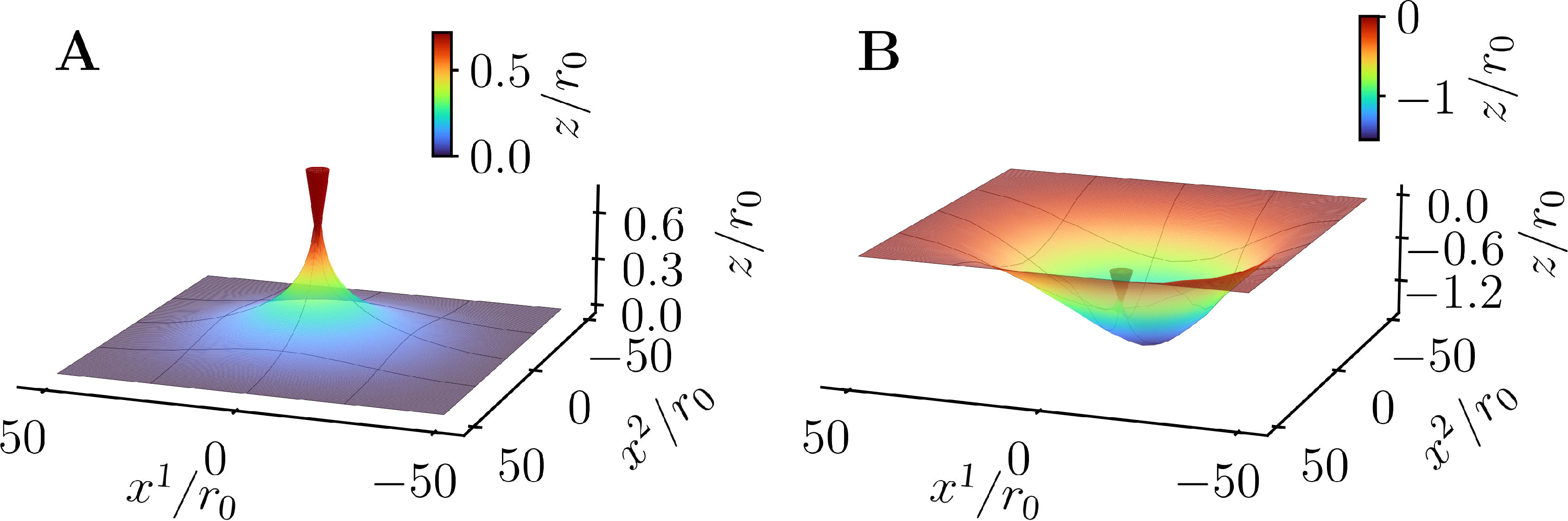
In what follows, we will focus on this regime, which is characterized by the presence of large gradients \(\omega \gg 1\). The prin displacement and contact angle may have the same or opposite sign, leading to distinct deformation responses; these two situations are presented in 3.
![Figure 3: Membrane shapes in the large-deformation regime, obtained with the irene [36]. A) Membrane deformation induced by a positive vertical displacement of the protein and positive contact angle, h_0 = 4.2 \, r_0 and \tan \alpha = 0.5, cf. 1. B) Membrane deformation induced by a negative vertical displacement of the protein and positive contact angle angle, h_0 = -6.5\, r_0, \tan \alpha = 0.5, cf. 1. The prins are depicted as red cones. A convergence analysis of such type of radially symmetric solution with respect to the finite-element mesh resolution is reported in [36].](/article/2601.15477/figure_1.png "fig:")
3.1.2 Solution with zero mean curvature↩︎
Analytical insights about the ld regime for the membrane can be obtained considering the following approximate solution.
In order to simplify the equation, it is convenient to introduce the quantity \(\psi\), by the relation \[\label{eq95sub95omega} \omega = \frac{\psi}{\sqrt{1-\psi^2}}.\tag{7}\] In 6, we show all geometrical quantities expressed in terms of \(\psi\) and its derivatives. Substituting 35 in 1 , we obtain: \[\begin{align} \tag{8} (1-\psi^2)\frac{\partial^2 H}{\partial r^2} + \left(\frac{1-\psi^2}{r}-\psi \frac{\partial \psi}{\partial r}\right)\frac{\partial H}{\partial r}+ \nonumber \\ \left(\frac{2\psi}{ r} \frac{\partial \psi}{\partial r} + \frac{1}{\ell}-2H^2\right)H=0 , \\ \tag{9} H = \frac{\partial \psi}{\partial r} + \frac{\psi}{r}. \end{align}\]
9 admits a solution with zero mean curvature, of the form \[\label{eq95zero95curvature} \psi = \frac{C_1}{r}.\tag{10}\] We observe that the two terms in the rhs of 9 are, respectively, the radial and angular curvature [40]. As a result, solution does not imply that \(z\) is linear in \(r\), i.e., that the radial curvature vanishes, but that the algebraic sum of radial and angular curvature is zero.
Although this solution is only valid for zero mean curvature, it constitutes an approximation of the exact solution in the general case where curvature is not zero. However, it allows for explicit, simple expressions of the membrane shape and height, which may be useful on a qualitative level. In particular, here we infer a relation between the contact angle \(\alpha\) and the corresponding spontaneous displacement of the protein. Indeed, substituting 10 in 7 , and integrating, we obtain that the corresponding profile of the membrane is: \[\label{eq95z95zero95curvature} z(r) = -C_1 \ln \Big(r -\sqrt{r^2-C_1^2}\Big) + C_2.\tag{11}\] 11 is the catenoid, a well known zero-curvature profile [18]. The integration constants \(C_1\) and \(C_2\) can be determined from the bcs , leading to: \[\label{eq95zero95curvature95solution} z(r) = - r_0 \sin{\alpha} \ln\frac{r - \sqrt{r^2-r_0^2\sin^2{\alpha}}}{R -\sqrt{R^2-r_0^2\sin^2{\alpha}}}.\tag{12}\] The displacement of the protein is then given by: \[\label{eq95zero95curvature951} h = - r_0 \sin{\alpha} \ln\frac{r_0 -r_0 \sqrt{1-\sin^2{\alpha}}}{R -\sqrt{R^2-r_0^2\sin^2{\alpha}}},\tag{13}\] For \(R \gg r_0\), 13 becomes \[\label{eq95displacement95zero95curvature} h \simeq - r_0\sin{\alpha}\left[\ln \frac{r_0}{R} + \ln\left(1 - \cos{\alpha}\right)\right]\tag{14}\] The comparison between the numerical solution obtained with irene and the zero-mean-curvature solution is shown in 4. The Figure shows that the zero-mean-curvature solution yields a reasonable approximation for the numerically exact solution, see 4.
![Figure 4: Comparison between the solution with zero mean curvature and the numerically exact, fe solution, in the large-deformation regime. The fe solution (thin black curves) has been obtained with the irene [36], and the zero-mean-curvature solution is shown as thick colored curves. Both solutions are shown for different values of the membrane radius R and contact angle \alpha.](/article/2601.15477/figure_3.png "fig:")
3.1.3 Forces↩︎
Another important feature in the interaction between the protein and the membrane is the force exerted by the membrane on the prin boundary. The expression for this force is derived in 7, and its tangential and normal components read \[\begin{align} \tag{15} {\boldsymbol{f}}_\perp & =2\kappa n^i\nabla_iH \\ \nonumber \tag{16} & = -2\kappa \frac{\partial {H}}{\partial {r}}, \\ {\boldsymbol{f}}_\parallel & =-n^i(2\kappa H^2+\sigma){\boldsymbol{e}}_i \end{align}\]
In the ld regime, the force exerted by the membrane on the protein has been evaluated numerically with irene; results are shown in 5. The force is found to be non-monotonic as a function of the membrane vertical displacement \(h\), and to depend on the size \(R\) of the membrane domain. Comparison of the curves in 5 with the solution found in [8] show qualitative adherence. The order of magnitude of the force is found to be in the range of \(1-10\) pN, which is the same order of magnitude of forces exerted by molecular motors and actin on the membrane [1]. Moreover, the presence of a maximum followed by a decrease may suggest the onset of instabilities in the dynamics, and points to nontrivial behavior in tubule formation and retraction.
![Figure 5: Force exerted by the membrane on a prin along the z-axis, in the large-deformation regime. The force has been computed numerically by using the irene [36]. Different panels show the force as a function of the membrane vertical displacement h, for different values of the size R of the membrane domain. A) R = 5 \, r_0, B) R = 10\, r_0, C) R =30\, r_0, D) R = 100\, r_0.](/article/2601.15477/figure_4.png "fig:")
3.1.4 Potential energy in a system with two proteins↩︎
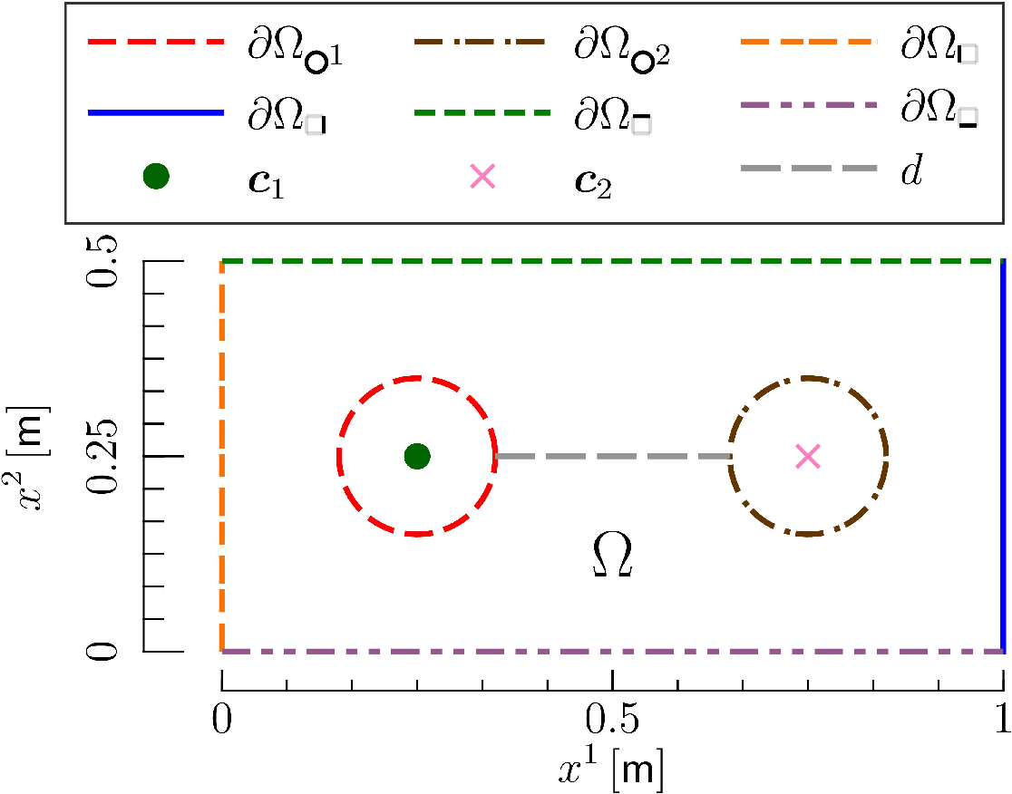
In what follows, we will focus on the membrane-mediated interaction between the two prins. We consider a square domain \(\Omega\) with side \(L\), containing two circular holes, which represent the two prins, see 6.
In this case, the rotational symmetry of 1 no longer holds. As a result, the pde cannot be reduced to an ode, and the analytical treatment of the problem is out of reach; we will thus study the solution numerically.
The centers of the two holes \({{\partial \Omega}_{{ {\mathord{ \tikz[baseline=-0.1ex]{ \draw[line width=1pt] (0,0) circle [radius=0.5ex]; } }}}1}}\), \({{\partial \Omega}_{{ {\mathord{ \tikz[baseline=-0.1ex]{ \draw[line width=1pt] (0,0) circle [radius=0.5ex]; } }}}2}}\) are located, respectively, at \({\boldsymbol{c}}_1 = (L/2 - d/2 - r_0, L/2)\) and \({\boldsymbol{c}}_2 = (L/2 + d/2 + r_0, L/2)\). Here, \(d\) is the distance between the two closest points on \({{\partial \Omega}_{{ {\mathord{ \tikz[baseline=-0.1ex]{ \draw[line width=1pt] (0,0) circle [radius=0.5ex]; } }}}1}}\) and \({{\partial \Omega}_{{ {\mathord{ \tikz[baseline=-0.1ex]{ \draw[line width=1pt] (0,0) circle [radius=0.5ex]; } }}}2}}\), and both prins have radius \(r_0\), see 6. We impose the following bcs: \[\begin{align} z & = 0 \text{ on } {\partial \Omega}_{\mathord{ \tikz[baseline=-0.1ex]{ \tikzmath{\size = 0.03ex; } \draw[line width=1pt] (0,0) -- (\size,0); \draw[line width=1pt] (\size,0) -- (\size,\size); \draw[line width=1pt] (\size,\size) -- (0ex,\size); \draw[line width=1pt] (0ex,\size) -- (0ex,0ex); } }}, \tag{17} \\ \nabla_i z & = -\tan \alpha \, \hat{r}_i \text{ on } {{\partial \Omega}_{{ {\mathord{ \tikz[baseline=-0.1ex]{ \draw[line width=1pt] (0,0) circle [radius=0.5ex]; } }}}^{1(2)}}}, \tag{18} \\ n^i \nabla_i z & = 0 \text{ on } {\partial \Omega}_{\mathord{ \tikz[baseline=-0.1ex]{ \tikzmath{\size = 0.03ex; } \draw[line width=1pt] (0,0) -- (\size,0); \draw[line width=1pt] (\size,0) -- (\size,\size); \draw[line width=1pt] (\size,\size) -- (0ex,\size); \draw[line width=1pt] (0ex,\size) -- (0ex,0ex); } }}, \tag{19} \end{align}\] where \(\hat{r}\) is the unit radius in the \(x^1\,x^2\) plane relative to the center of each prin.
![Figure 7: Profile of a membrane with two prins in the large-deformation regime, obtained using the irene [36]. A) Two prins with contact angles given by \tan \alpha_1 = \tan \alpha_2 = 0.6. B) Same as A, with \tan \alpha_1 = 0.6 and \tan \alpha_2 = -0.6.](/article/2601.15477/figure_5.png "fig:")
In the case where both proteins impose positive angles, this behavior can be attributed to the additional energy required to deform the membrane in the region between the two prins in order to satisfy the imposed angle constraint. This deformation induces significant curvature only over length scales shorter than the crossover length \(\ell\). On the other hand, when the distance between prins is of the order of the protein dimension \(r_0\), also the tilt of the phospholipids must be taken into account [16].
Given that the phospholipid tilt is not currently described by our model, in what follows we will assume the inter-protein distance to be larger than the prin radius, \(r_0\). To this end, we numerically compute the energy of the system [10] over a domain \(\Omega\) containing two proteins whose extension is much larger than \(d\): \[\label{eq95potential} U(d) \equiv \int_{\Omega} \left(\frac{\kappa}{2} H^2 + \sigma \right) \text{d} {S} - U_\infty,\tag{20}\] where \(\text{d} {S} \equiv \sqrt{\det g} dx^1 dx^2\) is the area element [40]. In 20 , \(U_\infty\) is the membrane potential \(U(d)\) for \(d \rightarrow \infty\).
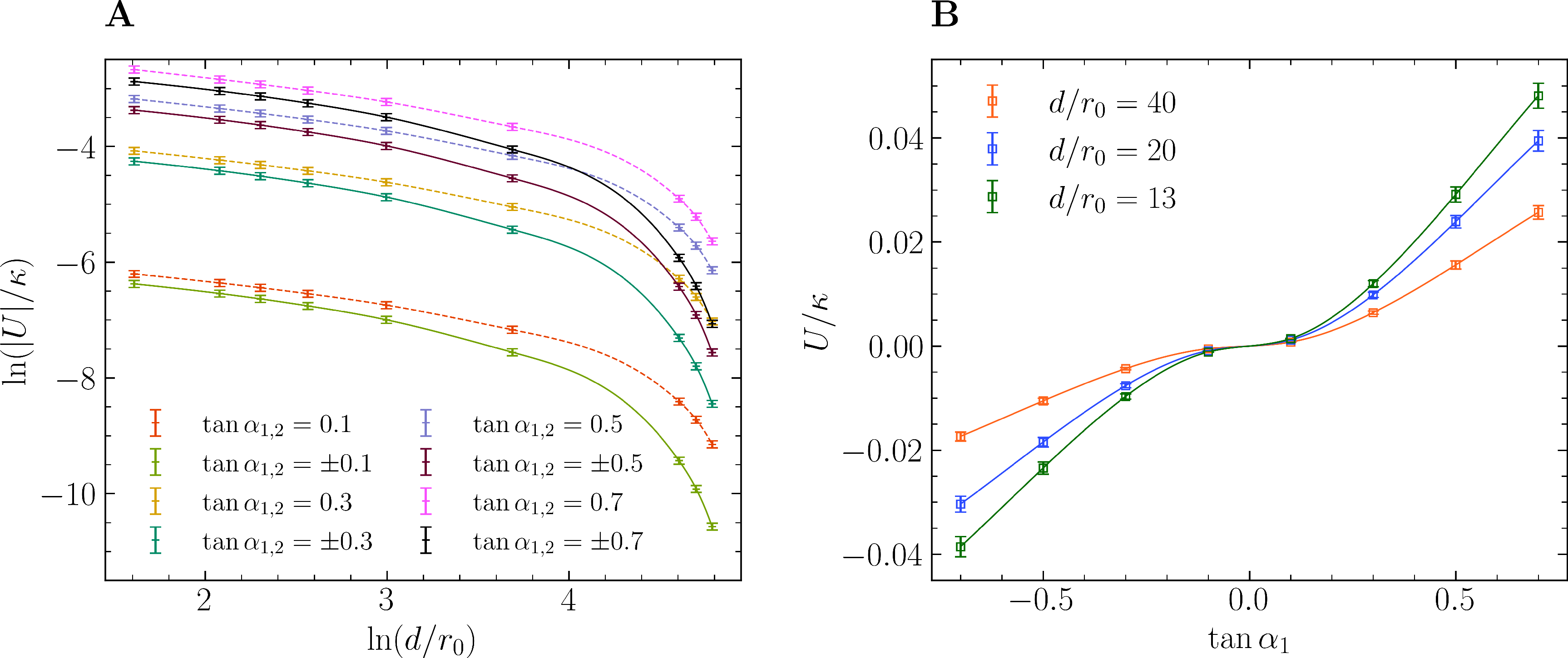
We considered prins with contact angles with the same or opposite orientations, see panels A and B, respectively, of 7. In addition, 8A shows the interaction potential as a function of the distance \(d\) between the two prins for different values of the contact angle. 8B displays the potential as a function of the contact angle of one of the two prins, while the other angle is held fixed. In
the Figure, the term \(U_\infty\) in 20 has been numerically evaluated setting the two prins at a distance \(d = 100 \, r_0\). As one can see from panel B in 8, the energy of the antisymmetric case is lower than that of the symmetric one. For this reason, in situations where both interaction types are allowed on the membrane, the system may exhibit an antiferromagnetic structure, which may give rise to patterns of alternating proteins.
3.2 Steady state with flows↩︎
In this Section, we will extend the analysis of 3.1 to include the presence of flows in the membrane.
The steady state with flows is described by the pdes \[\begin{align} \tag{21} \nabla_i v^i = & 0, \\ \tag{22} \rho \, v^j \nabla_j v^i = & \nabla^i \sigma + \eta \left( - \nabla_\text{\fontsize{7pt}{7pt}\selectfont{LB}}v^i + 2 K v^i \right) , \\ \nonumber \rho \, v^i v^j b_{ji} = & -2\kappa\left[ \nabla_i \nabla^i H + 2 H (H^2 - K) \right] + 2 \sigma H + \\ \tag{23} & 2 \eta (\nabla^i v^j)b_{ij} , \end{align}\] where \(b\) the second fundamental form [40] and \(\nabla_\text{\fontsize{7pt}{7pt}\selectfont{LB}}\) the Laplace-Beltrami operator, see [24], [41] for details.
We will consider a geometry given by a square domain with a circular hole, the prin, see 9. The reference frame is taken to be that of the prin; this means that the flow around the prin is studied as if the prin were stationary, and the surrounding fluid were moving. Importantly, here we assume that membrane deformations fall off at a distance from the prin comparable to the domain size \(L\), or larger.
In previous studies [24], [27], the Stokes equation was considered. However, in two-dimensional settings this leads to the well-known Stokes paradox, namely that solutions do not decay at infinity [50], [51]. This issue is typically resolved by introducing regularization mechanisms, most commonly through a coupling with a surrounding fluid.
In the present case, we retain the convective term, and neglect the effect of the external fluid. The latter assumption is justified as long as the characteristic length scale of flow-induced deformations, \(\lambda\), remains smaller than the Saffman–Delbrück length \(\lambda_\text{SD}\), which represents the scale at which viscous stresses within the membrane become comparable to those exerted by the surrounding fluid. The Saffman–Delbrück length is given by \(\lambda_\text{SD}= \eta / \eta_\text{3D}\), where \(\eta_\text{3D}\) is the viscosity of the external fluid (taken as \(\eta_\text{3D}= 10^{-3} \, \text{Pa}\sec\)). For the parameters considered in this work, \(\lambda_\text{SD}\) is of the order of \(10^{-5}\,\text{m}\), corresponding to approximately \(10^3 \, r_0\), which is one order of magnitude larger than the computational domain size \(L = 100\, r_0\).
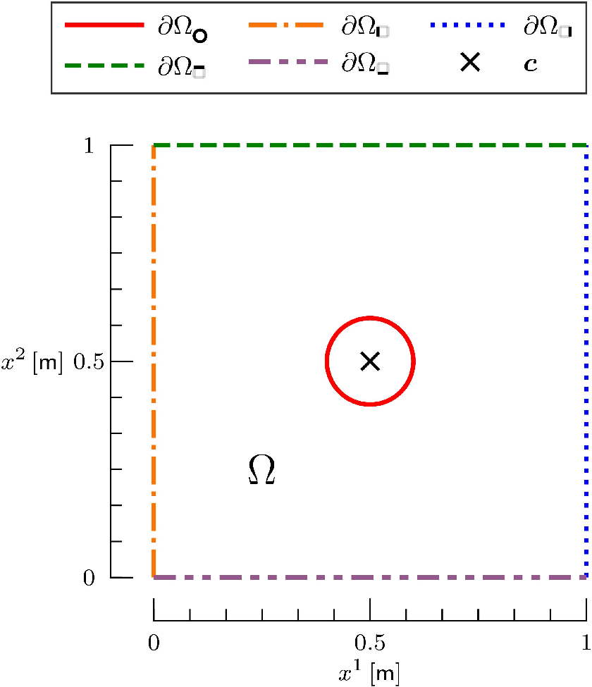
Given that the square boundary removes the rotational symmetry, the pdes can no longer be reduced to a set of odes, and a full numerical solution is needed. We numerically solve 21 22 23 by imposing the following bcs, see 9:
\[\begin{align} \tag{24} v^1 & = v_0 \text{ on } {\partial \Omega}_{ {\mathord{ \tikz[baseline=-0.1ex]{ \tikzmath{\size = 0.03ex; } \draw[line width=1pt, draw opacity = 0.15] (0,0) -- (\size,0); \draw[line width=1pt, draw opacity = 0.15] (\size,0) -- (\size,\size); \draw[line width=1pt, draw opacity = 0.15] (\size,\size) -- (0,\size); \draw[line width=1pt] (0,\size) -- (0,0); } }}}, \\ \tag{25} v^2 & = 0 \text{ on } {\partial \Omega}_{ {\mathord{ \tikz[baseline=-0.1ex]{ \tikzmath{\size = 0.03ex; } \draw[line width=1pt, draw opacity = 0.15] (0,0) -- (\size,0); \draw[line width=1pt, draw opacity = 0.15] (\size,0) -- (\size,\size); \draw[line width=1pt, draw opacity = 0.15] (\size,\size) -- (0,\size); \draw[line width=1pt] (0,\size) -- (0,0); } }}}, \\ \tag{26} v^1 & = 0 \text{ on } {{\partial \Omega}_{ {\mathord{ \tikz[baseline=-0.1ex]{ \draw[line width=1pt] (0,0) circle [radius=0.5ex]; } }}}}, \\ \tag{27} v^2 & = 0 \text{ on } {{\partial \Omega}_{ {\mathord{ \tikz[baseline=-0.1ex]{ \draw[line width=1pt] (0,0) circle [radius=0.5ex]; } }}}}, \\ \tag{28} \sigma & = \sigma_0 \text{ on } {\partial \Omega}_{ {\mathord{ \tikz[baseline=-0.1ex]{ \tikzmath{\size = 0.03ex; } \draw[line width=1pt, draw opacity = 0.15] (0,0) -- (\size,0); \draw[line width=1pt] (\size,0) -- (\size,\size); \draw[line width=1pt, draw opacity = 0.15] (\size,\size) -- (0,\size); \draw[line width=1pt, draw opacity = 0.15] (0,\size) -- (0,0); } }}}, \\ \tag{29} n_i \Pi^{i1} & = 0 \text{ on } {\partial \Omega}_{ {\mathord{ \tikz[baseline=-0.1ex]{ \tikzmath{\size = 0.03ex; } \draw[line width=1pt, draw opacity = 0.15] (0,0) -- (\size,0); \draw[line width=1pt] (\size,0) -- (\size,\size); \draw[line width=1pt, draw opacity = 0.15] (\size,\size) -- (0,\size); \draw[line width=1pt, draw opacity = 0.15] (0,\size) -- (0,0); } }}}, \\ \tag{30} n^i v_i & = 0 \text{ on } {\partial \Omega}_{ {\mathord{ \tikz[baseline=-0.1ex]{ \tikzmath{\size = 0.03ex; } \draw[line width=1pt] (0,0) -- (\size,0); \draw[line width=1pt, draw opacity = 0.15] (\size,0) -- (\size,\size); \draw[line width=1pt] (\size,\size) -- (0,\size); \draw[line width=1pt, draw opacity = 0.15] (0,\size) -- (0,0); } }}}, \\ \tag{31} \nabla_i z & = t_{ {\mathord{ \tikz[baseline=-0.1ex]{ \draw[line width=1pt] (0,0) circle [radius=0.5ex]; } }}}\hat{r}_i \text{ on } {{\partial \Omega}_{ {\mathord{ \tikz[baseline=-0.1ex]{ \draw[line width=1pt] (0,0) circle [radius=0.5ex]; } }}}}, \\ \tag{32} n^i \nabla_i z & = 0 \text{ on } {\partial \Omega}_{\mathord{ \tikz[baseline=-0.1ex]{ \tikzmath{\size = 0.03ex; } \draw[line width=1pt] (0,0) -- (\size,0); \draw[line width=1pt] (\size,0) -- (\size,\size); \draw[line width=1pt] (\size,\size) -- (0ex,\size); \draw[line width=1pt] (0ex,\size) -- (0ex,0ex); } }}, \\ \tag{33} z & = 0 \text{ on } {\partial \Omega}_{\mathord{ \tikz[baseline=-0.1ex]{ \tikzmath{\size = 0.03ex; } \draw[line width=1pt] (0,0) -- (\size,0); \draw[line width=1pt] (\size,0) -- (\size,\size); \draw[line width=1pt] (\size,\size) -- (0ex,\size); \draw[line width=1pt] (0ex,\size) -- (0ex,0ex); } }}. \end{align}\] In 29 , \(\Pi_{ij} \equiv - \sigma g_{ij} - \eta (\nabla_i v_j + \nabla_j v_i)\) is the membrane stress tensor [24], [41]. In 31 , \(\hat{r}\) is the unit radius in the \(x^1\,x^2\) plane relative to the prin center \(\boldsymbol{c}\), and we have set \[{\partial \Omega}_{\mathord{ \tikz[baseline=-0.1ex]{ \tikzmath{\size = 0.03ex; } \draw[line width=1pt] (0,0) -- (\size,0); \draw[line width=1pt] (\size,0) -- (\size,\size); \draw[line width=1pt] (\size,\size) -- (0ex,\size); \draw[line width=1pt] (0ex,\size) -- (0ex,0ex); } }}\equiv {\partial \Omega}_{ {\mathord{ \tikz[baseline=-0.1ex]{ \tikzmath{\size = 0.03ex; } \draw[line width=1pt, draw opacity = 0.15] (0,0) -- (\size,0); \draw[line width=1pt, draw opacity = 0.15] (\size,0) -- (\size,\size); \draw[line width=1pt, draw opacity = 0.15] (\size,\size) -- (0,\size); \draw[line width=1pt] (0,\size) -- (0,0); } }}}\cup {\partial \Omega}_{ {\mathord{ \tikz[baseline=-0.1ex]{ \tikzmath{\size = 0.03ex; } \draw[line width=1pt, draw opacity = 0.15] (0,0) -- (\size,0); \draw[line width=1pt] (\size,0) -- (\size,\size); \draw[line width=1pt, draw opacity = 0.15] (\size,\size) -- (0,\size); \draw[line width=1pt, draw opacity = 0.15] (0,\size) -- (0,0); } }}}\cup {\partial \Omega}_{ {\mathord{ \tikz[baseline=-0.1ex]{ \tikzmath{\size = 0.03ex; } \draw[line width=1pt] (0,0) -- (\size,0); \draw[line width=1pt, draw opacity = 0.15] (\size,0) -- (\size,\size); \draw[line width=1pt] (\size,\size) -- (0,\size); \draw[line width=1pt, draw opacity = 0.15] (0,\size) -- (0,0); } }}}.\]
The no-slip bcs reflect the assumption that phospholipids in direct contact with the protein are immobilized due to binding interactions [52]. [bc_flow_3,bc_flow_4] represent flow of membrane elements from \({\partial \Omega}_{ {\mathord{ \tikz[baseline=-0.1ex]{ \tikzmath{\size = 0.03ex; } \draw[line width=1pt, draw opacity = 0.15] (0,0) -- (\size,0); \draw[line width=1pt, draw opacity = 0.15] (\size,0) -- (\size,\size); \draw[line width=1pt, draw opacity = 0.15] (\size,\size) -- (0,\size); \draw[line width=1pt] (0,\size) -- (0,0); } }}}\), where the velocity field is assumed to be uniform and unperturbed by the prin. 28 reflects the hypothesis that \({\partial \Omega}_{ {\mathord{ \tikz[baseline=-0.1ex]{ \tikzmath{\size = 0.03ex; } \draw[line width=1pt, draw opacity = 0.15] (0,0) -- (\size,0); \draw[line width=1pt] (\size,0) -- (\size,\size); \draw[line width=1pt, draw opacity = 0.15] (\size,\size) -- (0,\size); \draw[line width=1pt, draw opacity = 0.15] (0,\size) -- (0,0); } }}}\) is far enough downstream of the protein that \(\sigma\) matches the unperturbed, intrinsic tension of the membrane, \(\sigma_0\). 30 enforces the presence of two ‘walls’ on the two sides of the boundary, through which membrane elements cannot flow. 31 enforces a fixed contact angle at the prin, reflecting binding between membrane phospholipids and the prin. 31 imposes that the membrane is flat at the outer boundary, according to the definition above of the length scale \(L\). Finally, 33 fixes the membrane height at the external boundary: This bc sets the reference height for the membrane profile, and it also reflects the assumption that membrane deformations decay at distances from the prin smaller than or equal to \(L\).
In 10 we display the resulting numerical solution obtained by using irene. The parameters used in 10 are \(v_0 = v_\ast\), where \[\label{eq95def95v} v_\ast\equiv \frac{\kappa}{L \eta},\tag{34}\] \(L = 10^2 \, r_0\), \(\sigma_0\) is given in 1, and \(t_{ {\mathord{ \tikz[baseline=-0.1ex]{ \draw[line width=1pt] (0,0) circle [radius=0.5ex]; } }}}= -0.3\).
The value of the characteristic velocity, \(v_\ast\), results from an adimensional number in 23 , i.e., the Scriven-Love number [25], [53], [54] \[S_\text{L}= \frac{\eta v L}{\kappa}.\] The value of \(v_\ast\) directly follows from setting \(S_\text{L}=1\). As shown in 11, the characteristic velocity \(v_\ast\) separates two different physical regimes:
\(v_0 < v_\ast\): The flow has no visible effect on the membrane shape, see 11A.
\(v_0 > v_\ast\): A membrane deformation induced by the flow appears, see 11B.
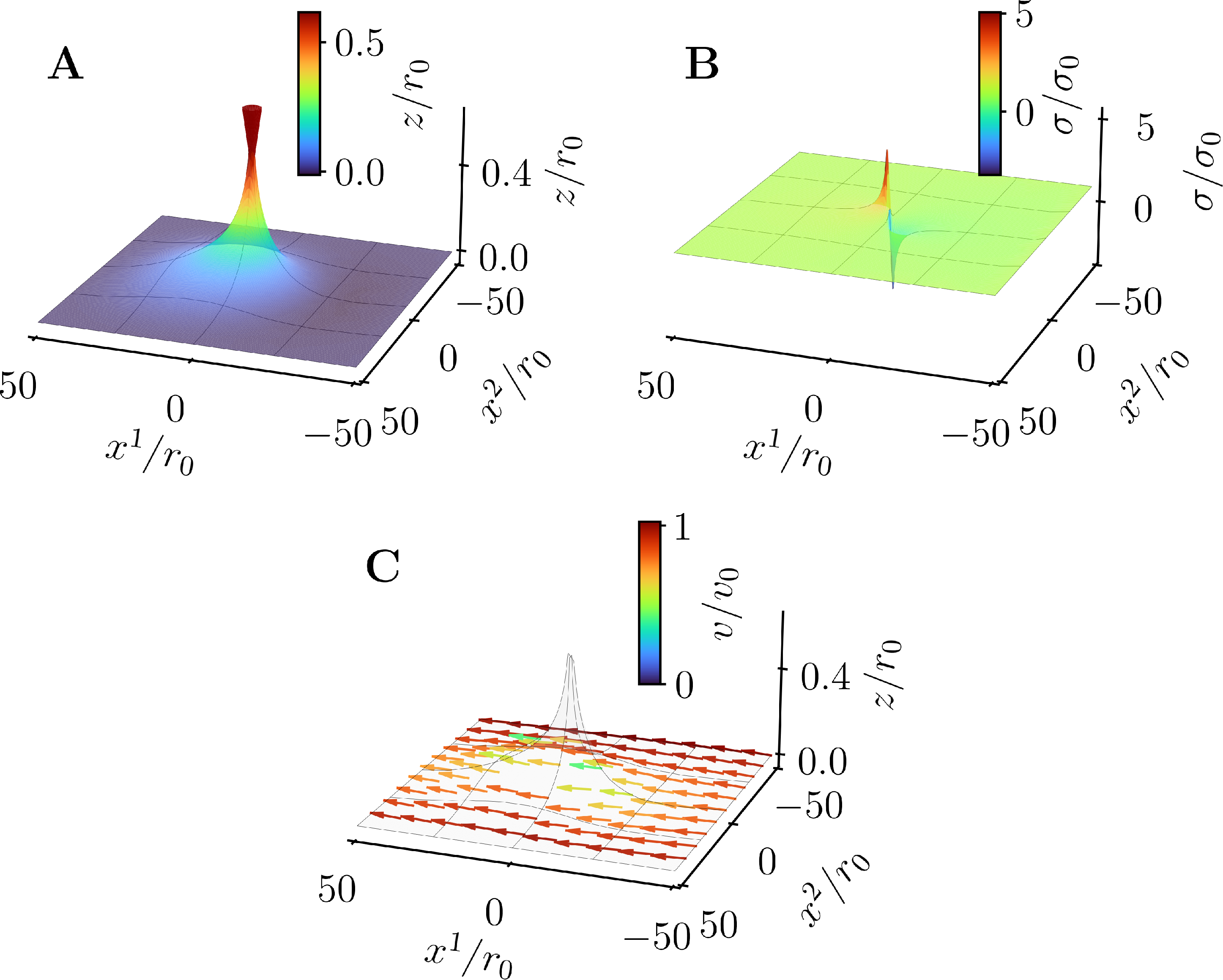
From the physical point of view, the existence of these regimes can be explained as follows. The characteristic length, or wavelength, \(\lambda\), of a flow-induced deformation for a given flow velocity \(v\), can be estimated by comparing the orders of magnitude of viscous and bending-rigidity effects. In fact, for a deformation of wavelength \(~\lambda\) to appear, the energy cost due to viscous effects, is larger than the bending rigidity cost if \(\lambda \eta v \gtrsim \kappa\). As a result, if \(v \gtrsim v_\ast\), a flow-induced deformation with wavelength \(\sim \kappa/(v \eta) < L\) appears. On the other hand, if \(v \lesssim v_\ast\), the flow-induced deformation wavelength would be larger than the domain size \(L\): Given that we assumed that no membrane deformations propagate to a distance equal or larger than \(L\) from the prin, see 33 32 , for these velocities no deformation can appear, see 11.
4 Discussion↩︎
We have studied, by combining analytical and numerical methods, the deformations in a cell membrane induced by prins in the ld regime. Our numerical analysis allows for going beyond current perturbative approaches [11]–[14], [20], [21], [23], which cannot describe the ld regime.
We first focused on the steady state of a lipid membrane with a single prin with axisymmetry, where the membrane is pinned on an outer circle with radius \(R\) and the prin is located at the center. We showed the limitations of perturbative solutions by comparing them to numerically exact, fe solutions [36], for large protein displacements or large prin contact angles, see 2. We developed an analytical solution for the shape equations in the ld regime, which assumes that the mean membrane curvature vanishes. Although this solution is only approximate, it yields a sensible, analytical expression of the membrane shape, see 4. According to this solution, a prin with a fixed contact angle has a spontaneous displacement that scales, for large \(R\), as \(\sim \ln R\), see 13 . Moreover, for a straight contact angle \(\alpha = \pi/2\), the spontaneous displacement remains finite, see 13 . We show that the vertical component of the force exerted by the membrane on the prin—the only nonzero component due to rotational symmetry—displays a non-monotonic dependence on the vertical displacement \(h\) of the prin. This behavior is analogous to the one obtained when a point-like force is applied to a membrane [8], demonstrating that the detailed size of the prin does not affect qualitatively the force profile.
We then analyzed the force exerted by the membrane on the prin, in the ld regime. The force displays a non-monotonic dependence on the vertical displacement of the prin, reminiscent of that of a point-like force applied to a membrane [8]. We assesses how this non-monotonic behavior is affected by the prin contact angle, as well as by the size of the membrane domain, see 5.
In addition, we numerically studied the membrane-mediated interaction between two prins in the ld regime. As shown in 8A, for the values of the inter-protein distance \(d\) that we considered, the potential does not display a power-law behavior. Instead, the potential shape shows a sub-power-law decay, i.e., it decreases with \(d\) slower than a power law. This nontrivial structure is due to the complex medium which conveys the interaction—the lipid membrane [55]. Finally, 8B shows that the potential is an odd function of the prin orientation, and that two prins with the same orientation yield a larger energy than two prins with opposite orientations. This behavior confirms the interpretation [12] that the angle imposed by each protein can be thought of as a ‘charge’, i.e., prins with the same and opposite orientations repel and attract each other, respectively.
In the presence of membrane flows, we identified the emergence of a characteristic velocity \(v_\ast\), of the order of a few microns per second, which reflects the competition between bending and viscous forces. At low velocities, membrane flows have negligible impact on membrane shape. On the other hand, at higher velocities, flow-induced deformations appear. We provided a theoretical estimate for the critical velocity at which this deformation arises, which explains their characteristic length and aligns well with numerical results. The presence of this characteristic velocity scale suggests that prins motion may significantly influence long-range membrane deformations and thus, for instance, membrane-mediated interactions.
An example of how flow-induced membrane deformations can influence interactions between prins is given by protein clustering on guvs. In this regard, we consider an example involving br—the best understood ion-transport protein [56]. Multiple br molecules have been
incorporated and diffuse [57] on the membrane of a guv [58]. A large guv with a \(\sim 100\, \mu \text{m}\) diameter populated with \(\sim 10^4\) brs, yields an average inter-protein distance \(d \sim 2 \, \mu \text{m}\). Given that the br lateral diffusion
coefficient of \(\sim 1.2 \, \mu \text{m}^2/\sec\), the typical values of br lateral diffusion velocity is \(v \sim 2 \, \mu
\text{m}/\sec\). According to the analysis of 3.2, this implies a flow-induced membrane deformation with wavelength \(\lambda \sim \kappa/(\eta v) \sim 1.5 \, \mu \text{m}\),
comparable with the inter-protein spacing. Given that this wavelength is comparable to the spacing between brs, flow-induced membrane deformations may imply a potential, significant
effect on br interactions and patterning on the guv surface.
Future work could leverage our results to study prin clustering in membranes. In fact, our analysis may be extended to study systems with more than two prins, examining how collective effects influence membrane deformation and forces, both with and without membrane flows. This analysis can also provide novel insights on prin clusters [55], [59], as well as on the effect of membrane-mediated forces on the cluster
assembly mechanisms and scaling laws. Finally, a full stability analysis of the governing equations may reveal the existence of flow-driven instabilities at larger velocities, with implications for membrane trafficking [2] and mechanosensitive processes in cells [60].
5 Acknowledgments↩︎
We would like to thank P. Bassereau, D. Lacoste, P. Sens and D. Wörthmuller for useful discussions.
6 Geometrical quantities for the zero-curvature solution↩︎
By substituting 7 the definitions of the geometrical quantities [39], we obtain \[\label{eq95geo95sub95omega95psi} \begin{align} \sqrt{\det g} = & \frac{r}{\sqrt{\psi^2+1}}, \\ g^{rr} = & 1+\psi^2, \\ g^{r\theta} = & 0, \\ g^{\theta \theta} = & 1, \\ H = & \frac{1}{2}\left(\frac{\partial \psi}{\partial r} + \frac{\psi}{r}\right), \\ K = & \frac{\psi}{ r} \frac{\partial {\psi}}{\partial {r}}. \end{align}\tag{35}\]
7 Variation of the Helfrich-Canhan’s energy functional↩︎
In order to find the line forces acting on the membrane boundary, we evaluate the variation of the Helfrich energy functional [10] to linear order under a perturbation of the membrane shape of the form \[\delta {\boldsymbol{X}} = {\boldsymbol{N}} \psi + {\boldsymbol{e}}_i \phi^i,\] where \(\boldsymbol{X}\) is the three-dimensional position vector of the membrane surface, \(\boldsymbol{N}\) is its normal and \({\boldsymbol{e}}_i\) the tangent vectors relative to the coordinate lines \(x^i\) [36], [39], [40]. Note that \(\boldsymbol{n}\) is a vector in three-dimensional Euclidean space, which is different from the normal \(n^i\) defined on the tangent bundle of the membrane manifold [36], see 3.1.1. Detailed calculation are presented in [39], the final result is: \[\begin{align} \delta \mathcal{H}[z] & = \int_\Omega \text{d} {S} \, [ \psi \left( 4\kappa H^3 - 2\sigma H - 4\kappa H K \right)+ \\ \nonumber & \nabla_i \phi^i \left( 2\kappa H^2 + \sigma \right) + 2\kappa H \nabla^i \nabla_i \psi ]. \end{align}\]
Multiple integrations by parts lead to \[\begin{align} \delta \mathcal{H}[z] = & \int_\Omega \text{d} {S} \, (4 \kappa H^3 - 2 H \sigma - 4 \kappa H K + \\ \nonumber & 2 \kappa \psi \nabla_i \nabla^i H) \, \psi + \\ \nonumber & \int_{\partial \Omega} \text{d} {l} \, 2\kappa [H n^i \nabla_i \psi - \psi n_i \nabla^i H + \\ \nonumber & + n_i \phi^i (2 \kappa H^2 + \sigma)]. \end{align}\]
The terms in the integral over the boundary \(\partial \Omega\) that are proportional to \(\psi\) and \(\phi^i\) represent the inverse of the line forces acting on the membrane boundary, that is 15 16 with exchanged sign.
References↩︎
Corresponding author: michele.castellana@curie.fr↩︎