Cost scaling of MPS and TTNS simulations for 2D and 3D systems with area-law entanglement
January 13, 2026
Abstract
Tensor network states are an indispensable tool for the simulation of strongly correlated quantum many-body systems. In recent years, tree tensor network states (TTNS) have been successfully used for two-dimensional systems and to benchmark quantum simulation approaches for condensed matter, nuclear, and particle physics. In comparison to the more traditional approach based on matrix product states (MPS), the graph distance of physical degrees of freedom can be drastically reduced in TTNS. Surprisingly, it turns out that, for large systems in \(D>1\) spatial dimensions, MPS simulations of low-energy states are nevertheless more efficient than TTNS simulations. With a focus on \(D=2\) and 3, the scaling of computational costs for different boundary conditions is determined under the assumption that the system obeys an entanglement (log-)area law, implying that bond dimensions scale exponentially in the surface area of the associated subsystems.
1 Introduction↩︎
Steve White’s density-matrix renormalization group (DMRG) [1]–[3] revolutionized the simulation of one-dimensional (1D) quantum many-body systems, allowing us to study properties of strongly-correlated ground states with very high accuracy – sometimes approaching machine precision. Although DMRG draws its conceptual inspiration from Wilson’s numerical renormalization group [4], [5] and quantum information theory, Östlund and Rommer [6], [7] showed that DMRG is a variational algorithm on matrix product states (MPS) [7]–[11], with the origins of MPS tracing back to the 1940s [8], [12]–[14]. Further MPS algorithms allow for the study of finite-temperature states, response functions, non-equilibrium dynamics, and driven-dissipative systems [15]–[33]. The entanglement properties of MPS are well-suited for 1D systems. One can prove that 1D states which obey an entanglement-entropy area law, such as ground states of gapped local systems, have faithful MPS approximations [34]–[37].
Natural extensions for \(D\geq 2\) spatial dimensions are projected entangled-pair states (PEPS) [38]–[42] and the multi-scale entanglement renormalization ansatz (MERA) [43], [44]. Both can represent states with area-law entanglement [41], [42], [45], [46] such that, for fixed approximation accuracy, bond dimensions \(M\) generally do not need to be increased with system size and grow at most polynomially for target states with log-area-law entanglement. However, while MPS computation costs are only \(\mathcal{O}(M^3)\), computation costs for 2D PEPS scale as \(\mathcal{O}(M^{10\dots 12})\) [47], [48] and as \(\mathcal{O}(M^{16\dots 26})\) for 2D MERA [49]–[51], which limits practicable bond dimensions \(M\) and the approximation accuracy. Furthermore, while MPS can be optimized and time-evolved with the very efficient and stable DMRG algorithms [1], [2], [11], [16], [29], [52], [53], optimization and evolution of MERA [54], [55] is slightly complicated by tensor isometry constraints, and the optimization and evolution of PEPS [47], [48], [56]–[59] is hampered by the inability to evaluate observables and gradients exactly [60], [61].
Tree tensor network states (TTNS) are a middle ground between MPS on the one hand and PEPS or MERA on the other hand. They are closely related to real-space renormalization group schemes [62]–[65] and had been considered in analytical work [66], [67], before TTNS were optimized using DMRG on tree graphs [68]–[70] and, finally, described and refined in the tensor-network formulation [71]–[75]. Compared to MPS, the maximal and average graph distances of physical sites are reduced from linear to logarithmic in the system size for TTNS, which is an important advantage. As both are classes of loop-free tensor networks, their associated varieties are closed sets [76] and the variational optimization is free of barren plateaus [77], [78]. While both can be optimized and evolved efficiently with DMRG and tangent-space algorithms, TTNS incur increased contraction costs of \(\mathcal{O}(M^{z+1})\), where \(z\) is the vertex degree.
In contrast to PEPS and MERA, MPS and TTNS do not match the area-law entanglement structure of typical systems in \(D\geq 2\) spatial dimensions [79]–[81]. Because of their lower contraction costs, algorithmic advantages and limited accessible bond dimensions \(M\) on current computers, MPS and TTNS are nevertheless competitive and often preferable for simulations of 2D and 3D systems. Many important works have employed MPS on cylinders and 2D strips [82]–[102]. In recent years, TTNS have become increasingly popular for the simulation of strongly correlated 2D and 3D systems in the context of condensed matter as well as nuclear and particle physics [72]–[75], [103]–[118].
This work compares the scaling of computational costs for MPS and TTNS simulations in \(D\geq 2\) spatial dimensions with target states that obey area laws in terms of Rényi entanglement entropies. As the algorithms for these tensor networks are very similar, the comparison is simply based on the time complexity per optimization or time-evolution step. Perhaps surprisingly, the results suggest that, in the limit of large system size \(L^D\), MPS (with a snake or helical mapping) are more efficient than TTNS with an exponential cost separation in \(L\). At least asymptotically, the increased contraction costs of TTNS outweigh the benefits of smaller graph distances.
Section 2 discusses the relation between MPS and TTNS bond dimensions and Rényi entanglement entropies for suitable bipartitions of the system, and Sec. 3 reviews tensor contraction costs for both types of tensor networks. Based on this, Secs. 4-6 determine and compare computational costs for the simulation of 2D, 3D, and higher-dimensional systems with MPS and binary TTNS, assuming entanglement (log-)area laws and covering different boundary conditions. In addition to summarizing the results, the conclusion in Sec. 7 briefly addresses neglected polynomial cost factors, total versus single-step costs, as well as the broader context concerning PEPS and MERA, applications beyond quantum physics, and tensor constraints.
2 Bond dimensions and subsystem entanglement↩︎
While also applicable to systems in continuous real space, let us consider quantum many-body systems on a lattice of \(N\) sites and single-site basis states \(\{|\sigma_x\rangle\,|\,\sigma_x=1,\dotsc,d_x\}\). We will assume the typical scenario, where tensor-network bond dimensions \(M_i\) are much larger than the site Hilbert-space dimensions \(d_x\), such that computational costs crucially depend on the scaling of bond dimensions with system size.
Extending prior work on MPS [36], [119], Ref. [37] showed that bond dimensions for MPS and TTNS approximations \(|\psi_\text{TN}\rangle\) of a target state \(|\psi\rangle\) can be bounded by \[\label{eq:Mbound} e^{S_{\tilde{\alpha},i}}(1-\delta)^{\frac{\tilde{\alpha}}{\tilde{\alpha}-1}} \leq M_i \leq e^{S_{\alpha,i}} \left(\frac{N-1}{\delta}\right)^{\frac{\alpha}{1-\alpha}}\!\!\!+1.\tag{1}\] Here, \(\delta:=\|\psi-\psi_\text{TN}\|^2\) denotes the approximation accuracy of the tensor network state \(|\psi_\text{TN}\rangle\) with bond dimensions \(\{M_i\}\), and \(S_{\alpha,i}=\frac{1}{1-\alpha}\ln\sum_\mu\lambda_{i,\mu}^{2\alpha}\) is the \(\alpha\)-Rényi entanglement entropy for the spatial bipartition \(\mathcal{A}_i\mathcal{B}_i\) of the system corresponding to cutting edge \(i\) of the tensor network with associated Schmidt coefficients \(\lambda_{i,1}\geq \lambda_{i,2}\geq\dotsc\geq 0\) of \(|\psi\rangle\). Specifically, Ref. [37] shows that any MPS or TTNS approximation with accuracy \(\delta\) obeys the lower bound in Eq. 1 and that there exist approximations of accuracy \(\delta\) with bond dimensions obeying the upper bound in Eq. 1 . We need \(\tilde{\alpha}>1\) for the lower bound and \(0<\alpha<1\) for the upper bound.
The central assumption of this work is that, for a given approximation accuracy, the relevant bond dimensions \(M_i\) of edges \(i\) in the tensor network scale up to polynomial prefactors as \[\label{eq:M-A} M_i\sim e^{c|\partial \mathcal{A}_i|} =: q^{|\partial \mathcal{A}_i|},\tag{2}\] where \(\mathcal{A}_i\) is the smaller of the two subsystems in the spatial bipartition \(\mathcal{A}_i\mathcal{B}_i\) of the system, arising from a cut at edge \(i\), and \(|\partial \mathcal{A}_i|\) is the surface area of that subsystem. According to the bounds 1 , the scaling 2 is a natural consequence of entanglement area and log-area laws, which are typically obeyed by ground and low-energy states of systems where interactions have a finite spatial range or decay sufficiently quickly with distance [79]–[81]. Intuitively, area laws \(S_{\alpha,i}\sim c|\partial \mathcal{A}_i|\) arise when all degrees of freedom that can contribute to entanglement between subsystem \(\mathcal{A}_i\) and its complement \(\mathcal{B}_i\) are located close to the subsystem interface due to an exponential spatial decay of correlations. In critical systems with diverging correlation lengths and power-law decay of correlations, there can be logarithmic corrections to the area law, resulting in polynomial prefactors in Eq. 2 , which are disregarded for the asymptotic scaling analysis in this work.
When reaching small subsystem sizes in the lower layers of TTNS – specifically, length scales smaller than the correlation length or comparable to lattice spacings – Eq. 2 may become quite inaccurate. However, we will find that, for large systems, the lower layers of TTNS have negligible contributions to the total computational costs such that these effects can be ignored.
3 MPS and TTNS contraction costs↩︎
![Figure 1: (a) Part of a TTNS with vertex degree z=3, orthogonality center x with edges 1,2,3, and the corresponding center tensor C_x, which has bond dimensions M_1,M_2,M_3. Arrows indicate isometric properties of tensors according to the convention of Ref. [37]. Vertical lines represent site-basis indices. The remaining panels show cost-dominant TTNS operations: (b) SVDs which yield Schmidt spectra \lambda_i, are used for truncations, and can move the orthogonality center, (c) contraction of Hamiltonian environment tensors \mathcal{E}_i and \tilde{\mathcal{E}}_i, where the square is a tensor of the Hamiltonian TTN operator with bond dimensions k_i, (d) contraction of C_x with its effective Hamiltonian H^\text{eff}_x, corresponding to the energy gradient \partial\langle\hat{H}\rangle/\partial C_x^\dagger.](/article/2601.08132/fig001.png "fig:")
The most costly operations in MPS optimization and time-evolution algorithms are singular value decompositions (SVD) and effective-Hamiltonian contractions [11], [53]. With \(M\times M\) matrices, the associated costs scale as \[\label{eq:cost-MPS} \mathcal{O}(M^3)\quad\text{for MPS}.\tag{3}\] Here and in the following, we do not specify costs for sums over Hamiltonian terms or, equivalently, bond indices of the Hamiltonian matrix product operator. These would add a factor that is polynomial in the size of the relevant subsystem \(\mathcal{A}_i\) and are disregarded in light of the exponential scaling 2 of the bond dimensions.
For a TTNS with vertex degree \(z\), computational costs of single-site algorithms generally scale as \[\label{eq:cost-TTNS-z} \mathcal{O}(M^{z+1})\quad\text{for TTNS}\tag{4}\] occurring, e.g., in the SVD of a tensor with \(z\) bond indices. We will hence focus the analysis on \(z=3\), i.e., binary TTNS. As in MPS algorithms, the most costly steps in TTNS algorithms are SVDs, the computation of energy gradients (effective-Hamiltonian contractions), and the propagation of environment tensors (effective Hamiltonians on branches of the tree); see Fig. 1. For a tensor with bond dimensions \(M_1,M_2,M_3\) all three operations have a cost of \[\label{eq:cost-TTNS} \mathcal{O}\big(M_1M_2(M_3)^2\big)\quad\text{for}\quad M_1\leq M_2\leq M_3.\tag{5}\] For SVDs, this follows when considering a matricization with indices \(M_1\) and \(M_2\) grouped into the matrix row index and \(M_3\) associated with the matrix column index. The costs for effective-Hamiltonian contractions and the propagation of environment tensors have the same scaling, because the associated tensor networks, as shown in Figs. 1c and 1d, arise from the same closed tensor network for the energy expectation value by removing one tensor (see Lemma 4 in Ref. [51]).
Note that the costs for (naive) two-site TTNS algorithms scale as \(\mathcal{O}(M^{3z-3})\) and should hence be avoided. However, half renormalization steps make it possible to reduce these costs of two-site TTNS algorithms to \(\mathcal{O}(M^{z+1})\) [74]. Alternatively, convergence problems of single-site algorithms can be circumvented by subspace expansion [120], [121]. According to recent algorithmic developments, the exponential scaling 4 of costs in the vertex degree \(z\) can be reduced to linear in \(z\) by imposing constraints on the tensor CP ranks [122], [123]. Nevertheless, for the purpose of this work, we will assume unconstrained tensors as this is currently the common choice in applications.
4 2D systems↩︎
4.1 Long cylinder↩︎
In MPS simulations for cylinders of length \(L_x\) and circumference \(L_y\equiv L\), we can arrange the MPS sites along a Hamiltonian path that covers the entire 2D lattice, following a trail that winds around the cylinder like a snake, fully traversing the system in the \(y\) direction before progressing in the \(x\) direction. See Figs. 2 and 3. One can also work in the limit \(L_x\to\infty\) by using infinite MPS [6], [10], [52], [124]–[126] with a repeating unit cell of \(\propto L\) different tensors. Cutting any edge \(i\) of the MPS splits the cylinder vertically into two segments \(\mathcal{A}_i\) and \(\mathcal{B}_i\) with an interface of size \(|\partial\mathcal{A}_i|\sim L\) such that MPS computation costs scale as \[\label{eq:2D-longCyl-MPS} \mathcal{O}(M_i^3)\stackrel{\eqref{eq:M-A}}{=}\mathcal{O}(q^{3L}).\tag{6}\]
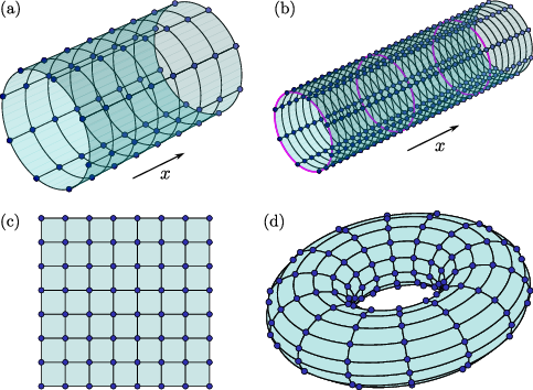
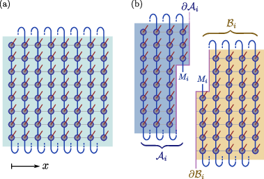
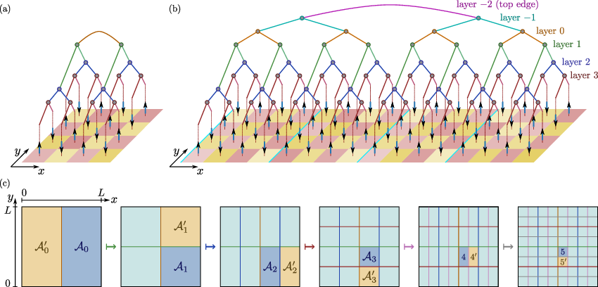
In simulations with binary TTNS, let us choose \(L_x=2^k L\) for simplicity. We then use the first \(k-1\) layers of the TTNS to split the cylinder into smaller cylinder segments of length \(2^{k-1}L\) in step 1, length \(2^{k-2}L\) in step 2, and so on until reaching \(L\times L\) cylinders in step \(k\) as shown in Fig. 4b for \(k=2\). In these steps, we have \(|\partial\mathcal{A}_i|\sim 2L\), corresponding to two interfaces of size \(\sim L\) at the right and left ends of each cylinder segment. The associated computational costs are \(\mathcal{O}(q^{8L})\) per contraction and SVD according to Eqs. 2 and 5 . We then proceed with layers \(0,1,2,\dotsc\) splitting each of the \(L\times L\) cylinder segments alternately in the \(x\) and \(y\) directions as indicated in Fig. 4 with associated subsystem surface areas \(|\partial\mathcal{A}_0|\sim 2L\), \(|\partial\mathcal{A}_1|\sim 2L\), \(|\partial\mathcal{A}_2|\sim \frac{3}{2}L\), \(|\partial\mathcal{A}_3|\sim L\), \(|\partial\mathcal{A}_4|\sim \frac{3}{4}L\), \(|\partial\mathcal{A}_5|\sim \frac{1}{2}L\) etc. So, the subsystem surface area is reduced by a factor \(1/2\) every two layers. See also Table ¿tbl:tab:2D?a.
In an optimization sweep or full time evolution step, we need to pass all tensors of the TTNS. While the number of tensors increases exponentially in the layer index \(n\), the subsystem surface areas \(|\partial\mathcal{A}_n|\) decrease exponentially in \(n\) such that, according to Eq. 2 , bond dimensions and computational costs per tensor decrease double-exponentially in \(n\). Hence, the total cost is dominated by tensor operations for the top layers and we arrive at the scaling \[\label{eq:2D-longCyl-TTNS} \mathcal{O}(M_0^2 M_1^2)\stackrel{\eqref{eq:M-A}}{=}\mathcal{O}(q^{8L}),\tag{7}\] for the total cost, which is substantially larger than the MPS cost 6 .
4.2 \(L\times L\) cylinder↩︎
In the comparison to TTNS, long cylinders are somewhat beneficial for MPS as increasing \(L_x\) only incurs a polynomial overhead. Let us now consider an \(L\times L\) cylinder, again with periodic boundary conditions (PBC) in the \(y\) direction. The MPS costs are still given by Eq. 6 . The top edge of the TTNS now corresponds to splitting the cylinder into two \(\frac{L}{2}\times L\) segments \(\mathcal{A}_0\) and \(\mathcal{A}_0'\) as shown in Figs. 4a and 4c. The corresponding boundary area is \(|\partial\mathcal{A}_0|=|\partial\mathcal{A}_0'|=L\) due to the open boundary conditions (OBC) in \(x\) direction. In layer 1, each of the cylinder segments is split horizontally, into two subsystems \(\mathcal{A}_1\) and \(\mathcal{A}_1'\) of size \(\frac{L}{2}\times \frac{L}{2}\) with surface area \(|\partial\mathcal{A}_1|=|\partial\mathcal{A}_1'|=\frac{3}{2}L\), leading to computational costs of \(\mathcal{O}\big(q^L(q^{\frac{3}{2}L})^3\big)=\mathcal{O}(q^{\frac{11}{2}L})\) per tensor according to Eqs. 2 and 5 . In layer 2, we split \(\mathcal{A}_1\) (and similarly all other layer-1 subsystems) further into subsystems \(\mathcal{A}_2\) and \(\mathcal{A}_2'\) of size \(\frac{L}{4}\times \frac{L}{2}\) with surface areas \(|\partial\mathcal{A}_2|=\frac{3}{2}L\) and \(|\partial\mathcal{A}'_2|=L\), where the asymmetry results from the OBC in \(x\) direction. One could try to optimize this splitting but, in the end, the TTNS computational costs scale as \[\label{eq:2D-cyl-TTNS} \mathcal{O}(M_0 M_1^3)\stackrel{\eqref{eq:M-A}}{=}\mathcal{O}(q^{\frac{11}{2} L}),\tag{8}\] which is substantially larger than the MPS cost 6 . See also Table ¿tbl:tab:2D?b.
4.3 \(L\times L\) square↩︎
| (a) Long cylinder | ||
| Layer | \(|\partial\A_n|\) | Cost |
| first \(k-1\) | \(2L\) | |
| 0 | \(2L\) | |
| 1 | \(2L\) | |
| 2 | \(\frac{3}{2}L\) | \(q^{7L}\) |
| 3 | \(L\) | \(q^{5L}\) |
| 4 | \(\frac{3}{4}L\) | \(q^{\frac{7}{2}L}\) |
| 5 | \(\frac{1}{2}L\) | \(q^{\frac{5}{2}L}\) |
| (b) \(L\times L\) cylinder | ||
| Layer | \(|\partial\A_n|\) | Cost |
| 0 (top edge) | \(L\) | – |
| 1 | \(\frac{3}{2}L\) | |
| 2 | \(\frac{3}{2}L\), \(L\) | |
| 3 | \(L\) | \(q^{5L}\) |
| 4 | \(\frac{3}{4}L\) | \(q^{\frac{7}{2}L}\) |
| 5 | \(\frac{1}{2}L\) | \(q^{\frac{5}{2}L}\) |
| (c) \(L\times L\) square (OBC) | ||
| Layer | \(|\partial\A_n|\) | Cost |
| 0 (top edge) | \(L\) | – |
| 1 | \(L\) | \(q^{4L}\) |
| 2 | \(\frac{5}{4}L\), \(\frac{3}{4}L\) | |
| 3 | \(L\), \(\frac{3}{4}L\) | |
| 4 | \(\frac{3}{4}L\) | \(q^{\frac{7}{2}L}\) |
| 5 | \(\frac{1}{2}L\) | \(q^{\frac{5}{2}L}\) |
| (d) \(L\times L\) torus | ||
| Layer | \(|\partial\A_n|\) | Cost |
| 0 (top edge) | \(2L\) | – |
| 1 | \(2L\) | |
| 2 | \(\frac{3}{2}L\) | \(q^{7L}\) |
| 3 | \(L\) | \(q^{5L}\) |
| 4 | \(\frac{3}{4}L\) | \(q^{\frac{7}{2}L}\) |
| 5 | \(\frac{1}{2}L\) | \(q^{\frac{5}{2}L}\) |
The PBC in \(y\) direction of the cylinders, that we considered so far, also benefit MPS as these PBC do not incur additional costs for MPS. Let us now consider an \(L\times L\) square system with OBC in both directions. Following our TTNS scheme of splitting subsystems alternately in the \(x\) and \(y\) directions, we find the associated boundary areas and costs per tensor as listed in Table ¿tbl:tab:2D?c. In layer 1, costs scale as \(\mathcal{O}(q^{4L})\), and one finds \(\mathcal{O}(q^{\frac{17}{4}L})=\mathcal{O}(q^{4.25 L})\) for layer 2 which, asymptotically, dominates the total cost. One might consider optimizing the splittings in layer 2 as, with the mentioned scheme, we get unequal boundary areas \(|\partial\mathcal{A}_2|=\frac{5}{4}L\) and \(|\partial\mathcal{A}'_2|=\frac{3}{4}L\). However, \(\mathcal{O}(q^{4 L})\) is a lower bound for the achievable cost per tensor, e.g., achieved when moving the interface of subsystems \(\mathcal{A}_2\) and \(\mathcal{A}_2'\) in Fig. 4c as far to the left as possible, i.e., when shaving off an infinitesimally thin slice at the left (inner) boundary of the \(\frac{L}{2}\times\frac{L}{2}\) subsystem \(\mathcal{A}_1\). The total TTNS cost hence scales as \[\label{eq:2D-square-TTNS} \mathcal{O}(M_1 M_2' M_2^2)\stackrel{\eqref{eq:M-A}}{=}\mathcal{O}(q^{4L \dots 4.25 L}).\tag{9}\]
4.4 \(L\times L\) torus↩︎
Finally, consider PBC in both directions for an \(L\times L\) system, i.e., a torus.
MPS simulations with PBC in the \(x\) direction with the same snake path shown in Fig. 3 are not trivial. When simply using an MPS with OBC – i.e., not introducing a tensor-network edge that connects the first and last MPS tensors – bond dimensions get essentially squared compared to the cylinder geometry and computational costs would increase from \(\mathcal{O}(q^{3L})\) in Eq. 6 to \(\mathcal{O}(q^{6L})\). Better methods for MPS with PBC and costs \(\mathcal{O}(q^{5L})\) and \(\mathcal{O}(q^{3L})\) have been introduced in Refs. [127] and [128], respectively, but come with some algorithmic complications. Assuming that PBC in the physical system are introduced to achieve \(x\) translation invariance and/or reduce finite-size effects, we can instead simply work with a long cylinder as discussed in Sec. 4.1 such that MPS computational costs are still \(\mathcal{O}(q^{3L})\). When sending \(L_x\to\infty\), we obtain infinite MPS [6], [10], [52], [124]–[126] and \(x\) translation invariance.
For TTNS on the \(L\times L\) torus, we can proceed as above. Splitting subsystems alternately in the \(x\) and \(y\) directions, we find the associated boundary areas and costs per tensor as listed in Table ¿tbl:tab:2D?d, resulting in a total TTNS cost of \[\label{eq:2D-torus-TTNS} \mathcal{O}(M_0 M_1^3)\stackrel{\eqref{eq:M-A}}{=}\mathcal{O}(q^{8 L}),\tag{10}\] which is again substantially larger than the MPS cost.
5 3D systems↩︎
5.1 Long cuboid with \(yz\) PBC↩︎
As a first case for 3D, consider cuboids of length \(L_x\), width \(L_y\equiv L\), and height \(L_z\equiv L\) using PBC for the \(y\) and \(z\) directions. As in 2D, we can arrange the MPS sites along a Hamiltonian path that covers the entire 3D lattice, following a trail that first covers a \(yz\) slice (constant or roughly constant \(x\), depending on details of the lattice) before progressing in the \(x\) direction to cover the next slice etc. One can work in the limit \(L_x\to\infty\) by using infinite MPS [6], [10], [52], [124]–[126]. Cutting any edge \(i\) of the MPS splits the cuboid along a \(yz\) slice into two segments \(\mathcal{A}_i\) and \(\mathcal{B}_i\) with an interface of size \(|\partial\mathcal{A}_i|\sim L^2\) such that MPS computational costs scale as \[\label{eq:3D-longCuboid-MPS} \mathcal{O}(M_i^3)\stackrel{\eqref{eq:M-A}}{=}\mathcal{O}(q^{3L^2}).\tag{11}\]
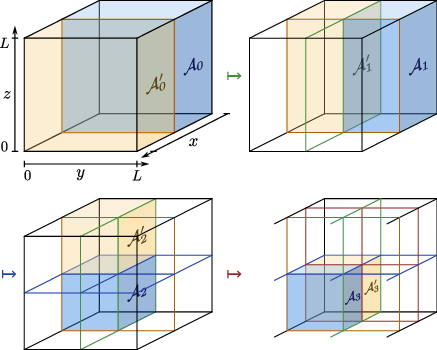
In simulations with binary TTNS, let us choose \(L_x=2^k L\). In analogy to Sec. 4.1, the first \(k-1\) layers of the TTNS split the cuboid into smaller cuboid segments \(\mathcal{A}_n\) of length \(2^{k-1}L\) in step 1, length \(2^{k-2}L\) in step 2, and so on until reaching \(L\times L\times L\) cubes in step \(k\). In these steps, we have \(|\partial\mathcal{A}_n|\sim 2L^2\), corresponding to two interfaces of size \(\sim L^2\) at the right and left ends of each cuboid segment. The associated computational costs are \(\mathcal{O}(q^{8L^2})\) per contraction and SVD according to Eqs. 2 and 5 . The subsequent layers \(0,1,2,\dotsc\) split each of the \(L\times L\times L\) cubes cyclically in the \(x\), \(y\), and \(z\) directions into subsystems of size \[\begin{align} |\mathcal{A}_0|&\sim\frac{L}{2}\times L\times L,\\ |\mathcal{A}_1|&\sim\frac{L}{2}\times \frac{L}{2}\times L,\\ |\mathcal{A}_2|&\sim\frac{L}{2}\times \frac{L}{2}\times \frac{L}{2},\\ |\mathcal{A}_3|&\sim\frac{L}{4}\times \frac{L}{2}\times \frac{L}{2},\\ |\mathcal{A}_4|&\sim\frac{L}{4}\times \frac{L}{4}\times \frac{L}{2},\\ |\mathcal{A}_5|&\sim\frac{L}{4}\times \frac{L}{4}\times \frac{L}{4},\quad \text{and so on} \end{align}\] as illustrated in Fig. 5. The associated subsystem surface areas are \(|\partial\mathcal{A}_0|\sim 2\ell_y\ell_z= 2L^2\), \(|\partial\mathcal{A}_1|\sim 2(\ell_y\ell_z+\ell_x\ell_z)=2L^2\), \(|\partial\mathcal{A}_2|\sim 2(\ell_y\ell_z+\ell_x\ell_z+\ell_x\ell_y)=\frac{3}{2}L^2\), \(|\partial\mathcal{A}_3|\sim L^2\), \(|\partial\mathcal{A}_4|\sim \frac{5}{8}L^2\), \(|\partial\mathcal{A}_5|\sim \frac{3}{8}L^2\), and so on, where surface areas \(|\partial\mathcal{A}_n|\) for all \(n\geq 2\) are given by the general formula \(2(\ell_y\ell_z+\ell_x\ell_z+\ell_x\ell_y)\) with the linear subsystem sizes \(\ell_x,\ell_y,\ell_z\). Hence, the subsystem surface area is reduced by a factor \(1/4\) every two layers. See also Table ¿tbl:tab:3D?a.
As discussed in Sec. 4.1, the total cost is dominated by tensor operations for the top layers and we arrive at the scaling \[\label{eq:3D-longCuboid-TTNS} \mathcal{O}(M_0^2 M_1^2)\stackrel{\eqref{eq:M-A}}{=}\mathcal{O}(q^{8L^2}),\tag{12}\] for the total cost, which is substantially larger than the MPS cost 11 .
| (a) Long cuboid with \(yz\) PBC | ||
| Layer | \(|\partial\A_n|\) | Cost |
| first \(k-1\) | \(2L^2\) | |
| 0 | \(2L^2\) | |
| 1 | \(2L^2\) | |
| 2 | \(\frac{3}{2}L^2\) | \(q^{7L^2}\) |
| 3 | \(L^2\) | \(q^{5L^2}\) |
| 4 | \(\frac{5}{8}L^2\) | \(q^{\frac{13}{4}L^2}\) |
| 5 | \(\frac{3}{8}L^2\) | \(q^{2L^2}\) |
| (b) Cube with \(yz\) PBC | ||
| Layer | \(|\partial\A_n|\) | Cost |
| 0 (edge) | \(L^2\) | – |
| 1 | \(\frac{3}{2}L^2\) | |
| 2 | \(\frac{5}{4}L^2\) | |
| 3 | \(L^2\), \(\frac{3}{4}L^2\) | \(q^{\frac{17}{4}L^2}\) |
| 4 | \(\frac{5}{8}L^2\) | \(q^{\frac{13}{4}L^2}\) |
| 5 | \(\frac{3}{8}L^2\) | \(q^{2L^2}\) |
| (c) Cube with \(xyz\) OBC | ||
| Layer | \(|\partial\A_n|\) | Cost |
| 0 (edge) | \(L^2\) | – |
| 1 | \(L^2\) | |
| 2 | \(\frac{3}{4}L^2\) | \(q^{\frac{7}{2}L^2}\) |
| 3 | \(\frac{3}{4}L^2\), \(\frac{1}{2}L^2\) | \(q^{\frac{11}{4}L^2}\) |
| 4 | \(\frac{9}{16}L^2\), \(\frac{7}{16}L^2\) | \(q^{\frac{5}{2}L^2}\) |
| 5 | \(\frac{3}{8}L^2\), \(\frac{5}{16}L^2\) | \(q^{\frac{29}{16}L^2}\) |
| (d) Cube with \(xyz\) PBC | ||
| Layer | \(|\partial\A_n|\) | Cost |
| 0 (edge) | \(2L^2\) | – |
| 1 | \(2L^2\) | |
| 2 | \(\frac{3}{2}L^2\) | \(q^{7L^2}\) |
| 3 | \(L^2\) | \(q^{5L^2}\) |
| 4 | \(\frac{5}{8}L^2\) | \(q^{\frac{13}{4}L^2}\) |
| 5 | \(\frac{3}{8}L^2\) | \(q^{2L^2}\) |
5.2 \(L^3\) cube with \(yz\) PBC↩︎
Consider now an \(L\times L\times L\) cube, again with PBC in the \(y\) and \(z\) directions. The MPS costs are still given by Eq. 11 . Again, we split cyclically in the \(x\), \(y\), and \(z\) directions such that the resulting subsystems \(\mathcal{A}_n\) for layer \(n=0,1,2,\dotsc\) are shaped as specified in Sec. 5.1 and Fig. 5, but the boundary areas \(|\partial\mathcal{A}_n|\) have changed due to the OBC in \(x\) direction. For example, \(|\partial\mathcal{A}_0|=\ell_y\ell_z=L^2\), \(|\partial\mathcal{A}_1|=\ell_y\ell_z+2\ell_x\ell_z=\frac{3}{2}L^2\), and \(|\partial\mathcal{A}_2|=\ell_y\ell_z+2(\ell_x\ell_z+\ell_x\ell_y)=\frac{5}{4}L^2\). In layer 3, we split \(\mathcal{A}_2\) (and similarly all other layer-2 subsystems) further into subsystems \(\mathcal{A}_3\) and \(\mathcal{A}_3'\) of size \(\frac{L}{4}\times \frac{L}{2}\times \frac{L}{2}\) with surface areas \(|\partial\mathcal{A}_3|=2(\ell_y\ell_z+\ell_x\ell_z+\ell_x\ell_y)=L^2\) and \(|\partial\mathcal{A}'_3|=\ell_y\ell_z+2(\ell_x\ell_z+\ell_x\ell_y)=\frac{3}{4}L^2\) with the asymmetry resulting from the OBC in \(x\) direction. One could try to optimize this splitting but, in the end, the TTNS computation costs scale as \[\label{eq:3D-cube-yz-TTNS} \mathcal{O}(M_0 M_1^3)\stackrel{\eqref{eq:M-A}}{=}\mathcal{O}(q^{\frac{11}{2} L^2}),\tag{13}\] which is substantially larger than the MPS cost 11 . See also Table ¿tbl:tab:3D?b.
5.3 \(L^3\) cube with \(xyz\) OBC↩︎
PBC in the \(yz\) directions do not affect the asymptotic cost for MPS, but they do increase the cost for TTNS. To see this explicitly, let us now consider an \(L\times L\times L\) cube with OBC in all directions. Following our TTNS scheme of splitting subsystems cyclically in the \(x\), \(y\), and \(z\) directions, we find the associated boundary areas and costs per tensor as listed in Table ¿tbl:tab:3D?c. Asymptotically, the total TTNS cost is dominated by the layer-1 cost \[\label{eq:3D-cube-TTNS} \mathcal{O}(M_0 M_1^3)\stackrel{\eqref{eq:M-A}}{=}\mathcal{O}(q^{4L^2}).\tag{14}\]
5.4 \(L^3\) cube with \(xyz\) PBC↩︎
Finally, consider PBC in all three directions for an \(L\times L\times L\) cube.
As discussed in Sec. 4.4, MPS simulations will be more efficient when not using PBC in the \(x\) direction but considering instead \(L_x\to\infty\) and using infinite MPS [6], [10], [52], [124]–[126]. With this approach or the algorithm from Ref. [128], the MPS costs are still \(\mathcal{O}(q^{3L^2})\) [Eq. 11 ].
For TTNS, we can proceed as above. Splitting subsystems cyclically in the \(x\), \(y\), and \(z\) directions, we find the associated boundary areas and costs per tensor as listed in Table ¿tbl:tab:3D?d, resulting in a total TTNS cost of \[\label{eq:3D-cube-xyz-TTNS} \mathcal{O}(M_0 M_1^3)\stackrel{\eqref{eq:M-A}}{=}\mathcal{O}(q^{8 L^2}),\tag{15}\] which is again substantially larger than the MPS cost.
6 \(L^D\) hypercube with PBC in \(D\geq 4\) dimensions↩︎
As a last scenario, consider a hypercube in \(D\) spatial dimensions with PBC in all directions.
For MPS, we can use the approach from Secs. 4.4 and 5.4. Either employing the method from Ref. [128], or sending \(L_x\to\infty\) and using OBC in the \(x\) direction instead of PBC, we achieve the cost scaling \[\label{eq:hypercube-MPS} \mathcal{O}(M_i^3)\stackrel{\eqref{eq:M-A}}{=}\mathcal{O}(q^{3L^{D-1}}).\tag{16}\]
For TTNS, both the original hypercube geometry as well as the modified geometry with \(L_x\to \infty\) and \(x\) OBC lead to the cost scaling \[\label{eq:hypercube-TTNS} \mathcal{O}(M_0 M_1^3)\stackrel{\eqref{eq:M-A}}{=}\mathcal{O}(q^{8L^{D-1}}).\tag{17}\] With (sub)system \(\mathcal{A}_0\) being an \(L^D\) hypercube, we then split cyclically in every spatial dimension when going through TTNS layers \(n=0,1,2,\dotsc\) With \(|\partial\mathcal{A}_0|=2L^{D-1}\) and \(|\partial\mathcal{A}_1|=|\partial\mathcal{A}'_1|=2L^{D-1}\), we obtain Eq. 17 .
7 Conclusion↩︎
Based on bounds for MPS and TTNS bond dimensions in terms of Rényi entanglement entropies [37], the determined scaling of computational costs as summarized in Table 1 suggests that MPS are more efficient than TTNS for the simulation of large systems in \(D\geq 2\) spatial dimensions with (log-)area-law entanglement. In terms of the system size, there is an exponential separation in the cost scaling, which is smallest for OBC and largest when applying PBC in all spatial directions. Some remarks are in order:
With computational costs scaling exponentially in surface areas \(\propto L^{D-1}\), we have disregarded polynomial computation-cost factors, which are due to (a) sums over Hamiltonian terms, (b) the numbers of tensors to be contracted, (c) log corrections to entanglement area laws in critical systems, and (d) polynomial terms in the bond-dimension bounds 1 . Such polynomial factors may give TTNS an advantage over MPS for small system sizes \(L\) but, according to the asymptotic scaling, there should then exist a crossover point \(L_\text{MPS}\) beyond which MPS are more efficient.
The comparison in this work is based on tensor contraction costs per optimization or time-evolution step. In principle, the required number of iterations for Krylov subspace methods for the local energy optimization in DMRG [1], [2], [11], [52], [73], [74] and for local time-evolution problems in the time-dependent variational principle [26], [53], [75] as well as the total number of sweeps in groundstate optimization may need to be increased with increasing system size to reach a certain accuracy. However, these numbers are usually system-size independent or chosen to be system-size independent in practical applications. The analysis in this work would also apply if these numbers scaled polynomially.
In the cost scaling analysis, we have assumed that the target state obeys a (log-)area law. In principle, intermediate states might have a different entanglement scaling. However, we can generally assume that the simulation spends most time in a regime where the entanglement scaling of the target state applies.
As mentioned in the introduction, TTNS and MPS with fixed bond dimensions do not match the area-law entanglement structure of typical systems in \(D\geq 2\) dimensions. PEPS and MERA do reproduce area laws [41], [42], [45], [46], but have much higher tensor contraction costs. Hence, there should be crossover points \(L_\text{PEPS}\) and \(L_\text{MERA}\), where PEPS and MERA become more efficient than MPS (and TTNS). A cost comparison between these methods is much more challenging and model-specific, as they require different optimization techniques.
Beyond applications in quantum physics, MPS and TTNS are also employed for machine learning [123], [129]–[133], the compression of deep neural networks [134]–[136], the approximation of high-dimensional probability distributions [137]–[140], and tensor completion in big-data analysis [141]–[143]. In these contexts, MPS and TTNS are frequently referred to as tensor trains and the hierarchical Tucker format, respectively [144]–[146]. Entanglement entropies are not immediately relevant in these cases and a cost comparison should be based on the scaling of measures like the mutual information, parameter redundancy, global self-similarity etc.
Finally, the presented analysis applies to the case of unconstrained tensors and would generally need adaptation for tensor networks with tensor constraints such as TTNS with CP-rank constraints [122], [123].
I thank Elizabeth Bennewitz, Zohreh Davoudi, Alexey Gorshkov, Caroline Jang, Hersh Kumar, Alessio Lerose, Federica Surace, and Nikita Zemlevskiy for discussions that motivated this work.
| Geometry | PBC | MPS cost | TTNS cost |
|---|---|---|---|
| 2D \(L\times L\) square | – | \(q^{3L}\) | \(q^{4L\dots 4.25L}\) |
| 2D \(L\times L\) cylinder | \(y\) | \(q^{3L}\) | \(q^{5.5L}\) |
| 2D \(L_x\times L\) cylinder, \(L_x\gg L\) | \(y\) | \(q^{3L}\) | \(q^{8L}\) |
| 2D \(L\times L\) torus | \(y,x\) | \(q^{3L*}\) | \(q^{8L}\) |
| 3D \(L\times L\times L\) cube | – | \(q^{3L^2}\) | \(q^{4L^2}\) |
| 3D \(L\times L\times L\) cube | \(z,y\) | \(q^{3L^2}\) | \(q^{5.5L^2}\) |
| 3D \(L_x\times L\times L\), \(L_x\gg L\) | \(z,y\) | \(q^{3L^2}\) | \(q^{8L^2}\) |
| 3D \(L\times L\times L\) cube | \(z,y,x\) | \(q^{3L^2*}\) | \(q^{8L^2}\) |
| \(D\)-dimensional \(L^D\) hypercube | all | \(q^{3L^{D-1}*}\) | \(q^{8L^{D-1}}\) |