Transmutation based Quantum Simulation for Non-unitary Dynamics
January 07, 2026
Abstract
We present a quantum algorithm for simulating dissipative diffusion dynamics generated by positive semidefinite operators of the form \(A=L^\dagger L\), a structure that arises naturally in standard discretizations of elliptic operators. Our main tool is the Kannai transform, which represents the diffusion semigroup \(e^{-AT}\), where \(T\) is the final simulation time, as a Gaussian-weighted superposition of unitary wave propagators. For target accuracy \(\varepsilon\), this representation leads to a linear-combination-of-unitaries implementation with a Gaussian tail and yields query complexity \(\tilde{O}(\sqrt{\|A\|\,T\,\log(1/\varepsilon)})\), up to the standard dependence on state-preparation and output-norm factors, improving the scaling in \(\|A\|,\,T\,\) and \(\varepsilon\) compared with generic Hamiltonian-simulation-based methods. We instantiate the method for the heat equation and biharmonic diffusion under non-periodic physical boundary conditions, and further use it as a subroutine for constant-coefficient linear parabolic surrogates arising in entropy-penalization schemes for the viscous Hamilton–Jacobi equations. In the long-time regime, and under a spectral-gap assumption, the same framework leads to a structured quantum linear solver by exploiting convergence to the steady state. In the normalized positive definite case, denoting by \(\kappa\) the condition number of \(A\), the solver outputs an \(\varepsilon\)-approximation to the quantum state proportional to \(A^{-1}\boldsymbol{b}\), using \(\widetilde{O}\!\left(\kappa^{3/2}\log^2(\kappa/\varepsilon)\right)\) calls to the block-encoding oracle.
Keywords: Kannai transform, Linear-combination-of-unitaries, Optimal query complexity, Linear solver
1 Introduction↩︎
Dissipative partial differential equations (PDEs), such as the heat equation and more general parabolic systems, are fundamental models for diffusion, relaxation, and transport across science and engineering. In high-dimensional regimes, classical discretization-based solvers may become computationally prohibitive, motivating alternative paradigms. Quantum computers can represent high-dimensional vectors as amplitude-encoded quantum states and, in principle, yield speedups for certain linear-algebraic primitives [1]–[4].
A core difficulty is that quantum hardware natively implements unitary time evolution, whereas diffusion is intrinsically non-unitary. This mismatch helps explain why Hamiltonian simulation—the simulation of Schrödinger dynamics—became an early and central target of quantum algorithms, leading to a mature toolkit with near-optimal complexity guarantees [5]–[14]. Designing quantum algorithms for dissipative dynamics therefore requires representing a non-unitary semigroup in terms of unitary primitives while retaining favorable dependence on the final time and the target accuracy.
Our approach. We propose a quantum algorithm based on the classical Kannai transformation (also known as transmutation or subordination) [15]–[17]. For generators of the form \[\mathcal{A}=\mathcal{L}^\dagger\mathcal{L}\succeq 0,\] the Kannai representation expresses the diffusion semigroup \(e^{-t\mathcal{A}}\) as a Gaussian-weighted superposition of unitary wave propagators associated with \(\mathcal{L}\). Algorithmically, we simulate the corresponding reversible dynamics and recover the diffusion solution by evaluating a Gaussian convolution in an auxiliary time variable.
This viewpoint is related to dilation-based wrap-and-average methods (e.g.Schrödingerization and its Fourier/contour variants), where the cost is governed by truncating an auxiliary kernel [12], [18]–[23]. The key quantitative distinction is that exponentially decaying kernels typically require truncation radii \(R=\Theta(T\log(1/\varepsilon))\), whereas the Gaussian Kannai kernel yields \(R=\Theta(\sqrt{T \log(1/\varepsilon)})\), improving the \(\varepsilon\)-and-\(T\)-dependence of the resulting algorithms.
Related work. Existing approaches to non-unitary simulation include: (i) discretize and solve via quantum linear system algorithms (QLSAs) [24]–[31]; (ii) dilate to a unitary PDE and apply Hamiltonian simulation [12], [18], [19], with closely related variants such as LCHS [20], [21] and contour-based matrix decomposition (CMD) [23]; and (iii) treat non-unitary generators via block-encoding or Lindbladian techniques [14], [32]. Our method belongs to the wrap-and-average family but exploits the Gaussian tail of the Kannai kernel to sharpen the dependence on \(\varepsilon\) for the structured class \(\mathcal{A}=\mathcal{L}^\dagger\mathcal{L}\).
Problem setting and contributions. We consider inhomogeneous linear evolution problems \[\label{eq:linear95eq} \frac{\mathrm{d}u}{\mathrm{d}t}=-\mathcal{A}u+f, \qquad u(0,\cdot)=u_0,\tag{1}\] where \(\mathcal{A}=\mathcal{L}^\dagger\mathcal{L}\) is self-adjoint and non-negative and \(f\) is a time-independent source. After spatial discretization, this yields a matrix \(A=L^\dagger L\). We assume standard quantum access to the discretized operators via block-encodings and to the input data via state preparation (see Section 4).
Our main contributions are as follows.
Kannai-based quantum simulation of diffusion. We combine the Gaussian decay of the Kannai kernel with high-order quadrature in the auxiliary variable, the linear-combination-of-unitaries (LCU) framework, and near-optimal Hamiltonian simulation to obtain a quantum algorithm for 1 . The query complexity to a block-encoding of the Hermitian dilation Hamiltonian scales as \[\widetilde{O}\!\bigl(u_r\,\sqrt{T\|A\|\log(1/\varepsilon)}\bigr),\] where \(T\) is the final time, \(\varepsilon\) is the target precision, and \(u_r\) captures the relative size of the input and forcing. Up to polylogarithmic factors, this improves the dependence on \(\varepsilon\), \(T\), and \(\|A\|\) compared with wrap-and-average methods based on exponentially decaying kernels.
PDE instantiations and boundary conditions. We apply the framework to the heat equation and biharmonic diffusion, and show that Dirichlet and Neumann boundary conditions can be handled without changing the leading-order complexity under standard sparse discretizations on bounded domains.
A structured quantum linear solver from long-time dynamics. In the strongly dissipative regime, we solve \(A\boldsymbol{x}=\boldsymbol{b}\) with \(A=L^\dagger L\) by running the dynamics to \(T=\Theta(\kappa\log(1/\varepsilon))\) and applying the Kannai-based simulator. This yields a quantum linear solver with query complexity \[\widetilde{O}\bigl(\kappa^{3/2}\log^2(\kappa/\varepsilon)\bigr),\] improving over early HHL-type algorithms and direct inverse block-encodings with naive postselection, which have quadratic condition-number dependence in standard formulations.
Further transmutation constructions. We collect additional transmutation-based reductions representing target dynamics as superpositions of reversible evolutions, including algorithms for second-order-in-time models (e.g.Euler–Poisson–Darboux via spherical means) and an alternative reduction from the heat equation to unitary transport via transport–heat averaging.
Organization. Section 2 reviews transmutation and rewrites it as a first-order Hamiltonian system suitable for quantum simulation. Section 3 presents discretization, Gaussian quadrature, and error analysis. Section 4 gives the quantum implementation and query bounds, and Section 5 illustrates them on heat, viscous Hamilton–Jacobi, and biharmonic diffusion. Section 6 addresses the long-time regime and the induced linear solver. Section 7 collects additional transmutation-based constructions. Section 8 presents numerical experiments that validate the correctness of the Kannai-transform–based LCU method. Conclusions are in Section 9.
Notation. For \(j\in[N]\), \(| j \rangle\in\mathbb{C}^N\) denotes the \(j\)th computational basis vector. For any nonzero vector \(\boldsymbol{u}\), \(| \boldsymbol{u} \rangle:=\boldsymbol{u}/\|\boldsymbol{u}\|_2\) denotes the associated normalized amplitude-encoded quantum state. Thus bold symbols denote unnormalized vectors, while kets denote normalized quantum states unless stated otherwise. We write \(\widetilde{O}(\cdot)\) to suppress polylogarithmic factors, and use \(O(\cdot)\) with constants independent of the problem parameters of interest. All logarithms are natural.
2 Transmutation and unitary superpositions↩︎
Transmutation methods provide a systematic way to represent one evolution problem as a superposition of another, often simpler, evolution whose analysis or numerical treatment is more accessible. We refer to [33]–[38] for representative developments. In this section we use transmutation techniques to express a target non-unitary dynamics as a superposition of unitary evolutions. This structure is particularly suitable for quantum algorithm design.
2.1 Kannai transformation for the linear system↩︎
We consider the setting in which the spatial operator admits the factorization \[\label{eq:operator32A} \mathcal{A} = \mathcal{L}^{\dagger}\mathcal{L},\tag{2}\] together with boundary conditions that make \(\mathcal{A}\) nonnegative and self-adjoint. A prototypical example is \(\mathcal{L}=-\nabla\) as a map from \(H^1_0(\Omega)\) to \(L^2(\Omega)\). In this case \(\mathcal{A}=-\Delta_x\) with homogeneous Dirichlet boundary conditions. We study the linear system with a time-independent source term \[\label{eq:diffu32u} \frac{\mathrm{d}u (t,x)}{\mathrm{d}t} = -\mathcal{A}u(t,x) + f(x), \qquad u(0,x)=u_0(x).\tag{3}\]
Kannai [15] shows that one can represent \(u\) via a transmutation operator acting only on the time variable: \[\label{eq:Hw} u(t,x) = (\mathcal{H}w)(t,x) = \int_{\mathbb{R}} K(t,s)\,w(s,x)\,\mathrm{d}s.\tag{4}\] The kernel is Gaussian, \[\label{eq:Gaussian32kernel} K(t,s) = \frac{1}{\sqrt{4\pi t}}\,e^{-s^{2}/(4t)}.\tag{5}\] The auxiliary function \(w\) solves the inhomogeneous wave-type equation \[\label{eq:w-wave-A-LL} w_{ss}(s,x) = -\mathcal{A}w(s,x) + f(x), \qquad w(0,x)=u_0(x),\quad w_s(0,x)=0.\tag{6}\]
2.2 Unitary embedding via first-order factorization↩︎
To reveal the unitary dynamics underlying 6 , we recast the second-order equation as a first-order system. Introduce an auxiliary variable \(v\) by \[\frac{\mathrm{d}}{\mathrm{d}s}v(s,x) = -\mathcal{L}w(s,x), \qquad v(0,x)=0.\] Define the augmented state, the embedded source term, and the block operator by \[\label{eq:def32psi-wv} \boldsymbol{\psi}(s,x) = [\,w(s,x)\;\, v(s,x)\,]^{\top}, \qquad \widetilde{\boldsymbol{f}}(x) = [\,f(x)\;\, 0\,]^{\top}, \qquad \widetilde{\mathcal{L}} = \begin{bmatrix} 0 & \mathcal{L}^{\dagger} \\ -\mathcal{L} & 0 \end{bmatrix}.\tag{7}\] A direct calculation shows that \(\boldsymbol{\psi}\) satisfies the inhomogeneous first-order system \[\label{eq:p} \frac{\mathrm{d}}{\mathrm{d}s}\boldsymbol{\psi}(s,x) = \widetilde{\mathcal{L}}\,\boldsymbol{\psi}(s,x) + s\,\widetilde{\boldsymbol{f}}(x), \qquad \boldsymbol{\psi}(0,x)=\boldsymbol{\psi}_0(x),\tag{8}\] where \(\boldsymbol{\psi}_0(x)=[\,u_0(x),\,0\,]^{\top}\). By Duhamel’s principle, 8 admits the variation-of-constants formula \[\label{eq:unitary32dynamics} \boldsymbol{\psi}(s,x) = \mathcal{U}(s)\,\boldsymbol{\psi}_0(x) + \int_0^{s}\sigma\,\mathcal{U}(s-\sigma)\,\widetilde{\boldsymbol{f}}(x)\, \mathrm{d}\sigma, \qquad \mathcal{U}(s)=\exp\bigl(\widetilde{\mathcal{L}}s\bigr).\tag{9}\] The operator \(\widetilde{\mathcal{L}}\) is skew-adjoint under the boundary conditions inherited from \(\mathcal{L}\). Consequently, the homogeneous evolution \(\mathcal{U}(s)\) is unitary. This unitary structure will be central in our quantum constructions.
The next lemma makes explicit that the transmutation formula expresses \(u\) as an integral superposition of the unitary dynamics generated by \(\widetilde{\mathcal{L}}\).
Lemma 1. Let \(\mathcal{A}=\mathcal{L}^{\dagger}\mathcal{L}\) be a nonnegative self-adjoint operator independent of time. Assume that \(u\) and \(w\) satisfy 3 and 6 , respectively. Let \(\mathcal{H}\) be the transmutation operator in 4 with kernel 5 . Then \[\label{eq:u-from-w-short} u(t,x) = \Pi_1 \Bigg( \int_{\mathbb{R}} K(t,s)\,\mathcal{U}(s)\,\boldsymbol{\psi}_0(x)\,\mathrm{d}s + \int_{\mathbb{R}} K(t,s)\, \int_0^{s} \sigma\,\mathcal{U}(s-\sigma)\,\widetilde{\boldsymbol{f}}(x)\, \mathrm{d}\sigma\,\mathrm{d}s \Bigg),\tag{10}\] where \(\Pi_1\) denotes the projection onto the first component, \(\boldsymbol{\psi}_0\) and \(\widetilde{\boldsymbol{f}}\) are defined in 7 , and \(\mathcal{U}(s)\) is given by 9 .
3 Numerical discretization↩︎
In this section we construct a fully discrete formulation of the proposed representation. We discretize the first-order system in space to obtain a semi-discrete unitary evolution, then approximate the resulting Gaussian integrals by quadrature and derive error bounds.
3.1 Spatial discretization of the first-order system↩︎
To discretize 8 in space, we introduce a matrix \(L\in\mathbb{C}^{N\times N}\) arising from an appropriate spatial discretization of the differential operator \(\mathcal{L}\). Let \(\boldsymbol{w}_h(s),\boldsymbol{v}_h(s)\in\mathbb{C}^{N}\) denote the semi-discrete approximations of \(w(s,\cdot)\) and \(v(s,\cdot)\), and let \(\boldsymbol{f}_h\in\mathbb{C}^{N}\) be the discrete source term. Define the stacked state vector and forcing vector by \[\label{eq:psi95b} \boldsymbol{\psi}_h(s)= \begin{bmatrix} \boldsymbol{w}_h(s)\\[1mm]\boldsymbol{v}_h(s) \end{bmatrix}\in\mathbb{C}^{2N}, \qquad \boldsymbol{\psi}_0= \begin{bmatrix} \boldsymbol{u}_0\\ \boldsymbol{0} \end{bmatrix}\in\mathbb{C}^{2N}, \qquad \boldsymbol{b}= \begin{bmatrix} \boldsymbol{f}_h\\ \boldsymbol{0} \end{bmatrix}\in\mathbb{C}^{2N},\tag{11}\] where \(\boldsymbol{u}_0\) is the discrete initial data. The semi-discrete system can be written as \[\label{eq:discrete-system} \frac{\mathrm d}{\mathrm ds}\boldsymbol{\psi}_h(s) = \widetilde{L}\boldsymbol{\psi}_h(s) + s\boldsymbol{b} =: -iH\,\boldsymbol{\psi}_h(s)+s\boldsymbol{b},\tag{12}\] with the anti-Hermitian matrix \(\widetilde{L}\) and its Hermitian counterpart \(H\) given by \[\label{eq:H-Sch-short} \widetilde{L}= | 0 \rangle\langle 1 |\otimes L^{\dagger} - | 1 \rangle\langle 0 |\otimes L \in\mathbb{C}^{2N\times 2N}, \qquad H=i\widetilde{L}.\tag{13}\] Hence the homogeneous propagator \(U(s):=\exp(-iHs)\) is unitary. By Duhamel’s principle, the solution of 12 admits the representation \[\label{eq:psi-duhamel} \boldsymbol{\psi}_h(s) = U(s)\boldsymbol{\psi}_0 +\left(\int_0^s (s-\sigma)\,U(\sigma)\,\mathrm d\sigma\right)\boldsymbol{b}.\tag{14}\]
Based on 14 , we define the discrete target at time \(T>0\) by the Kannai Gaussian integral \[\begin{align} \boldsymbol{u}_f^{\mathrm{disc}}(T) &:=\int_{\mathbb{R}} K(T,s) \,\boldsymbol{\psi}_h(s)\,\mathrm ds \notag \\ &= \big(\int_{\mathbb{R}}\kappa_T(s)\,U(s)\,\mathrm ds\big)\boldsymbol{\psi}_0 +\big(\int_{\mathbb{R}}\kappa_T(s) \int_0^{s} (s-\sigma)\,U(\sigma)\,\mathrm d\sigma\,\mathrm ds\big)\boldsymbol{b} \label{eq:I1I2} \end{align}\tag{15}\] with \[\label{eq:kappa} \kappa_T(s)=K(T,s) =(4\pi T)^{-1/2}e^{-s^2/(4T)}.\tag{16}\] We also introduce the Gaussian tail function \[\Phi_T(a) :=\frac{1}{\sqrt{4\pi T}}\int_a^\infty e^{-s^2/(4T)}\,\mathrm ds =\tfrac12\,\mathrm{erfc}\!\left(\frac{a}{2\sqrt{T}}\right).\] Since \(U(s)\) is unitary and \(\kappa_T\) is integrable on \(\mathbb{R}\), all integrals above are absolutely convergent, and Fubini’s theorem applies. Exchanging the order of integration gives the one-dimensional representation. More precisely, one obtains \[\label{eq:vf95disc} \boldsymbol{u}_f^{\mathrm{disc}}(T) = \left(\int_{\mathbb{R}} \kappa_T(s)\,U(s)\,\mathrm ds\right)\boldsymbol{\psi}_0 +\left(\int_{\mathbb{R}} \Lambda_T(\sigma)\,U(\sigma)\,\mathrm d\sigma\right)\boldsymbol{b},\tag{17}\] where the scalar kernel \(\Lambda_T\) is given by \[\label{eq:Lamda} \Lambda_T(\sigma)= \begin{cases} \displaystyle \frac{1}{\sqrt{4\pi T}}\int_{\sigma}^{\infty} e^{-s^2/(4T)}(s-\sigma)\,\mathrm ds = \sqrt{\frac{T}{\pi}}\,e^{-\sigma^2/(4T)}-\sigma\,\Phi_T(\sigma), & \sigma\ge 0,\\[10pt] \displaystyle \frac{1}{\sqrt{4\pi T}}\int_{-\infty}^{\sigma} e^{-s^2/(4T)}(\sigma-s)\,\mathrm ds = \sqrt{\frac{T}{\pi}}\,e^{-\sigma^2/(4T)}+\sigma\,\Phi_T(-\sigma), & \sigma<0. \end{cases}\tag{18}\] It follows directly from this formula that \(\Lambda_T\) is nonnegative and even. Moreover, \(\int_{\mathbb{R}}\Lambda_T(\sigma)\,d\sigma =T\).
3.2 Numerical integration↩︎
For numerical implementation, we truncate the infinite integration domain to a finite interval \([-R,R]\) with \(R>0\). We partition \([-R,R]\) into uniform panels of length \(h_1>0\). Let \(M_R:=R/h_1\) and assume that \(M_R\) is an integer. The panels are indexed by \(m=-M_R,\dots,M_R-1\) and given by \([mh_1,(m+1)h_1]\). On each panel we apply a \(Q\)-point Gauss–Legendre rule. Let \(\{x_q,\omega_q\}_{q=1}^{Q}\) be the standard Gauss–Legendre nodes and weights on \([-1,1]\). The corresponding nodes and rescaled weights on \([mh_1,(m+1)h_1]\) are \[\label{eq:weight95and95points} s_{q,m}=\frac{h_1}{2}x_q+\frac{2m+1}{2}h_1, \qquad w_{q,m}=\frac{h_1}{2}\omega_q, \qquad q=1,\dots,Q.\tag{19}\]
We assume that the kernel values can be precomputed offline to high precision. More precisely, we use approximations \(\kappa_T^a\) and \(\Lambda_T^a\) satisfying \[\label{eq:kappa95Lambda95approxi} |\kappa_T^a(s)-\kappa_T(s)|\le \delta_{\mathrm{off}}\,|\kappa_T(s)|,\quad |\Lambda_T^a(s)-\Lambda_T(s)|\le \delta_{\mathrm{off}}\,|\Lambda_T(s)|, \quad \forall s\in\mathbb{R}.\tag{20}\] With these ingredients, the quadrature approximations of the two integrals in 17 lead to the discrete representation \[\label{eq:uf95h} \boldsymbol{u}_f^{\mathrm{disc}}(T)\approx \boldsymbol{u}_f^{h}(T) = \sum_{m=-M_R}^{M_R-1}\sum_{q=1}^{Q} \Bigl( c_{q,m}\,U(s_{q,m})\,\boldsymbol{\psi}_0 +d_{q,m}\,U(s_{q,m})\,\boldsymbol{b} \Bigr),\tag{21}\] where \[\label{eq:coeffs} c_{q,m}=w_{q,m}\,\kappa_T^a(s_{q,m}), \qquad d_{q,m}=w_{q,m}\,\Lambda_T^a(s_{q,m}).\tag{22}\]
Remark 1. The offline precomputation of \(\kappa_T\) and \(\Lambda_T\) removes the need to evaluate nested integrals during the online stage. Both contributions in 17 reduce to one-dimensional weighted sums over quadrature nodes. Alternative quadrature rules such as the trapezoidal rule or Monte Carlo sampling can be incorporated analogously. The choice of quadrature affects the required coefficient precision but does not change the final query complexity of the quantum procedure, since coefficient precision enters only polylogarithmically in the relevant qubit complexity.
3.3 Error analysis for the fully discrete quadrature↩︎
We estimate the error of the fully discrete quadrature scheme approximating \(\boldsymbol{u}_f^{\mathrm{disc}}(T)\) by \(\boldsymbol{u}_f^{h}(T)\): \[\mathcal{E} = \|\boldsymbol{u}_f^{h}(T)-\boldsymbol{u}_f^{\mathrm{disc}}(T)\|.\] The error consists of three contributions: (i) truncation of the integral to \([-R,R]\), (ii) Gauss–Legendre quadrature discretization on each panel, and (iii) offline approximation of the kernel functions.
The following theorem provides a complete error bound together with explicit parameter choices.
Theorem 1. Assume that the offline kernels \(\kappa_T^a\) and \(\Lambda_T^a\) satisfy the relative accuracy condition 20 . Let \(\boldsymbol{u}_f^{h}(T)\) denote the truncated quadrature approximation 21 and \(\boldsymbol{u}_f^{\mathrm{disc}}(T)\) the target representation 17 . Then, for any \(\epsilon\in(0,1)\), there exist parameters \(R>0\), \(Q\ge1\), \(h_1>0\), and \(\delta_{\mathrm{off}}>0\) such that \[\|\boldsymbol{u}_f^{h}(T)-\boldsymbol{u}_f^{\mathrm{disc}}(T)\| \le \epsilon\bigl(\|\boldsymbol{\psi}_0\|+T\|\boldsymbol{b}\|\bigr).\] Moreover, the total coefficient magnitudes satisfy \[\sum_{m,q}|c_{q,m}|\le 1+\epsilon, \qquad \sum_{m,q}|d_{q,m}|\le (1+\epsilon)T+\epsilon .\]
In particular, the above bounds hold under the explicit choices \[R =2\sqrt{T\log\!\Big(\frac{8}{\epsilon}\Big)} =O\!\big(\sqrt{T\log(1/\epsilon)}\big),\] and \[Q=O\big(\log(1/\epsilon)\big), \qquad h_1\le \frac{1}{e\bigl(\|L\|+1/\sqrt{2T}\bigr)}, \qquad \delta_{\mathrm{off}}\le\epsilon/4 .\]
Proof. We decompose the error into truncation, quadrature, and offline approximation errors. Define the exact and truncated integral operators by \[\begin{align} \mathcal{K}_T &:=\int_{\mathbb{R}}\kappa_T(s)U(s)\,\mathrm ds, & \mathcal{M}_T &:=\int_{\mathbb{R}}\Lambda_T(s)U(s)\,\mathrm ds,\\ \mathcal{K}_{T,R} &:=\int_{-R}^{R}\kappa_T(s)U(s)\,\mathrm ds, & \mathcal{M}_{T,R} &:=\int_{-R}^{R}\Lambda_T(s)U(s)\,\mathrm ds . \end{align}\] The corresponding composite Gauss–Legendre approximations with exact kernels are \[\mathcal{K}_{T,R}^{Q} :=\sum_{m=-M_R}^{M_R-1}\sum_{q=1}^{Q} w_{q,m}\kappa_T(s_{q,m})U(s_{q,m}),\quad \mathcal{M}_{T,R}^{Q} :=\sum_{m=-M_R}^{M_R-1}\sum_{q=1}^{Q} w_{q,m}\Lambda_T(s_{q,m})U(s_{q,m}),\] and the offline-kernel versions are \[\mathcal{K}_{T,R}^{Q,a} :=\sum_{m=-M_R}^{M_R-1}\sum_{q=1}^{Q} w_{q,m}\kappa_T^a(s_{q,m})U(s_{q,m}),\quad \mathcal{M}_{T,R}^{Q,a} :=\sum_{m=-M_R}^{M_R-1}\sum_{q=1}^{Q} w_{q,m}\Lambda_T^a(s_{q,m})U(s_{q,m}).\] Then \[\boldsymbol{u}_f^{h}(T)-\boldsymbol{u}_f^{\mathrm{disc}}(T) = (\mathcal{K}_{T,R}^{Q,a}-\mathcal{K}_T)\boldsymbol{\psi}_0 + (\mathcal{M}_{T,R}^{Q,a}-\mathcal{M}_T)\boldsymbol{b} .\] It remains to bound the two operator differences \(\mathcal{K}_{T,R}^{Q,a}-\mathcal{K}_T\) and \(\mathcal{M}_{T,R}^{Q,a}-\mathcal{M}_T\). For instance, \[\|\mathcal{K}_{T,R}^{Q,a}-\mathcal{K}_T\| \le \|\mathcal{K}_T-\mathcal{K}_{T,R}\| + \|\mathcal{K}_{T,R}-\mathcal{K}_{T,R}^{Q}\| + \|\mathcal{K}_{T,R}^{Q}-\mathcal{K}_{T,R}^{Q,a}\|,\] and the same decomposition holds for the \(\mathcal{M}\)-term.
3.3.0.1 Truncation
Since \(U(s)\) is unitary, the homogeneous truncation error is bounded by the Gaussian tail. With \(x=R/(2\sqrt T)\), \[\|\mathcal{K}_T-\mathcal{K}_{T,R}\| \le \int_{|s|>R}\kappa_T(s)\,\mathrm ds = \operatorname{erfc}(x) \le \frac{e^{-x^2}}{\sqrt{\pi}x}.\] For the inhomogeneous kernel, formula 18 gives \(\Lambda_T\ge0\), \(\Lambda_T\) even, and \(\int_{\mathbb{R}}\Lambda_T(\sigma)\,\mathrm d\sigma=T.\) Moreover, by Fubini’s theorem, \[\int_{|\sigma|>R}\Lambda_T(\sigma)\,\mathrm d\sigma = \int_R^\infty \kappa_T(s)(s-R)^2\,\mathrm ds \le \frac{T}{\sqrt{\pi}x^3}e^{-x^2}.\] Thus, for \[R=2\sqrt{T\log(8/\epsilon)},\] up to changing the universal numerical constant in the logarithm, the truncation contribution is bounded by \[O(\epsilon)\bigl(\|\boldsymbol{\psi}_0\|+T\|\boldsymbol{b}\|\bigr).\]
3.3.0.2 Quadrature
Let \[B:=\|H\|+\frac{1}{\sqrt{2T}} = \|L\|+\frac{1}{\sqrt{2T}}.\] On each panel, \(\kappa_T(s)U(s)\) is analytic. The kernel \(\Lambda_T\) is analytic on the two half-lines, and the point \(0\) is a panel endpoint, so the same composite Gauss–Legendre estimate applies branchwise. The standard Gauss–Legendre remainder estimate, together with \(\|\partial_s^rU(s)\|\le \|H\|^r\) and the Gaussian derivative bounds, yields \[\|\mathcal{K}_{T,R}-\mathcal{K}_{T,R}^{Q}\| \le Ce^{-cQ}, \qquad \|\mathcal{M}_{T,R}-\mathcal{M}_{T,R}^{Q}\| \le CTe^{-cQ},\] provided \[h_1\le\frac{1}{eB} = \frac{1}{e(\|L\|+1/\sqrt{2T})}.\] Here \(C,c>0\) are universal constants independent of \(T\), \(\|L\|\), and \(\epsilon\). Choosing \[Q=C_0\log(1/\epsilon)\] with \(C_0\) sufficiently large makes the quadrature contribution \[O(\epsilon)\bigl(\|\boldsymbol{\psi}_0\|+T\|\boldsymbol{b}\|\bigr).\]
3.3.0.3 Offline kernel approximation
By the relative accuracy assumption 20 and the unitarity of \(U(s)\), \[\|\mathcal{K}_{T,R}^{Q}-\mathcal{K}_{T,R}^{Q,a}\| \le \delta_{\mathrm{off}} \sum_{m,q}w_{q,m}\kappa_T(s_{q,m}), \quad \|\mathcal{M}_{T,R}^{Q}-\mathcal{M}_{T,R}^{Q,a}\| \le \delta_{\mathrm{off}} \sum_{m,q}w_{q,m}\Lambda_T(s_{q,m}).\] The scalar versions of the preceding truncation and quadrature estimates imply \[\sum_{m,q}w_{q,m}\kappa_T(s_{q,m})\le 1+C\epsilon, \qquad \sum_{m,q}w_{q,m}\Lambda_T(s_{q,m})\le T(1+C\epsilon)+C\epsilon .\] Hence, with \(\delta_{\mathrm{off}}\le\epsilon/4\), after absorbing universal constants into the parameter choices, the offline contribution is also bounded by \[O(\epsilon)\bigl(\|\boldsymbol{\psi}_0\|+T\|\boldsymbol{b}\|\bigr).\] Combining the three estimates gives \[\|\boldsymbol{u}_f^{h}(T)-\boldsymbol{u}_f^{\mathrm{disc}}(T)\| \le \epsilon\bigl(\|\boldsymbol{\psi}_0\|+T\|\boldsymbol{b}\|\bigr).\]
Finally, we bound the coefficient magnitudes. Since the quadrature weights are positive and \(\kappa_T,\Lambda_T\ge0\), \[\sum_{m,q}|c_{q,m}| \le (1+\delta_{\mathrm{off}}) \sum_{m,q}w_{q,m}\kappa_T(s_{q,m}) \le 1+\epsilon.\] Similarly, \[\sum_{m,q}|d_{q,m}| \le (1+\delta_{\mathrm{off}}) \sum_{m,q}w_{q,m}\Lambda_T(s_{q,m}) \le (1+\epsilon)T+\epsilon.\] This proves the stated error and coefficient bounds. ◻
4 Quantum implementation and query complexity↩︎
In this section we present the quantum implementation of our method for the inhomogeneous system in 3 and derive the resulting query complexity bounds.
For the quantum implementation we flatten the double index \((q,m)\) into a single index \(j\in\{0,\dots,M-1\}\), where \(M=2M_RQ\). We write \[c_j := c_{q,m}, \qquad d_j := d_{q,m}, \qquad s_j := s_{q,m}.\] Since the same quadrature nodes are used for both sums, the discrete representation 21 becomes \[\label{eq:uf-disc-flat-short} \boldsymbol{u}_f^h = \sum_{j=0}^{M-1} \bigl( c_j\,U(s_j)\,\boldsymbol{\psi}_0 + d_j\,U(s_j)\,\boldsymbol{b} \bigr),\tag{23}\] where \(U(s)=\exp(-iHs)\) and \(H\) is given in 13 .
4.1 Block-encoding of the Hamiltonians↩︎
We work in the standard sparse-query/block-encoding model [10], [39], [40]. Assume access to an \((\alpha_L,a_L,0)\)-block-encoding of \(L\), namely a unitary \(U_L\) such that \[\label{eq:L-block-short} (\langle 0^{a_L} |\otimes I_N)\,U_L\,(| 0^{a_L} \rangle\otimes I_N)=\frac{L}{\alpha_L}, \qquad \alpha_L\ge \|L\|.\tag{24}\] Then \(U_L^\dagger\) block-encodes \(L^\dagger\) with the same parameters. We emphasize that access to a factor \(L\) is natural for standard staggered or mixed discretizations, where \(L\) corresponds to a discrete gradient/flux operator, and is not an additional assumption beyond assembling the PDE operator \(A = L^{\dagger} L\).
Define the Hermitian dilation \[\widetilde{H}_0:=| 0 \rangle\!\langle 1 |\otimes L^\dagger+| 1 \rangle\!\langle 0 |\otimes L .\] Using one additional “position” qubit and \(U_L,U_L^\dagger\), one can construct a unitary \(W_{H_0}\) acting on \(a_H:=a_L+1\) ancillas and the \(2N\)-dimensional signal space such that \[\label{eq:H0-block-final-short} (\langle 0^{a_H} |\otimes I_{2N})\,W_{H_0}\,(| 0^{a_H} \rangle\otimes I_{2N}) =\frac{\widetilde{H}_0}{\alpha_L}.\tag{25}\] With \(P:=| 0 \rangle\!\langle 0 |-i| 1 \rangle\!\langle 1 |\), one has \(H=(P\otimes I_N)\widetilde{H}_0(P^\dagger\otimes I_N)\). Define \[\label{eq:UH-def-correct} \mathrm{HAM}_H:=(I_{a_H}\otimes P\otimes I_N)\,W_{H_0}\,(I_{a_H}\otimes P^\dagger\otimes I_N).\tag{26}\] Then \(\mathrm{HAM}_H\) is an \((\alpha_H,a_H,0)\)-block-encoding of \(H\) with \(\alpha_H=\Theta(\alpha_L)\), and each call to \(\mathrm{HAM}_H\) uses \(O(1)\) queries to \(U_L\) and \(U_L^\dagger\).
Let \(s_{\max}:=\max_j |s_j|\le R\) and set \(\gamma_j:=s_j/s_{\max}\in[-1,1]\). Using reversible arithmetic, we implement scalar-preparation oracles \(O_{\gamma,\mathrm{L}}\) and \(O_{\gamma,\mathrm{R}}\) such that, conditioned on \(| j \rangle\), they prepare amplitudes and phases for \(\gamma_j\): \[\label{eq:gamma-oracle} \begin{align} O_{\gamma,\mathrm{L}}:\;| j \rangle| 0 \rangle_\gamma &\mapsto | j \rangle\!\left(\sqrt{|\gamma_j|}| 0 \rangle_\gamma+\sqrt{1-|\gamma_j|}| 1 \rangle_\gamma\right),\\ O_{\gamma,\mathrm{R}}:\;| j \rangle| 0 \rangle_\gamma &\mapsto | j \rangle\!\left(e^{i\theta_j^{(\gamma)}}\sqrt{|\gamma_j|}| 0 \rangle_\gamma+\sqrt{1-|\gamma_j|}| 1 \rangle_\gamma\right). \end{align}\tag{27}\] The resulting overhead is polylogarithmic in the target precision. With these, define the unitary \(\mathrm{HAM}_{H_s}\) by \[\label{eq:U-scalar-def} \begin{align} \mathrm{HAM}_{H_s} :={}&\, I_M \otimes \Bigl( \bigl(O_{\gamma,\mathrm{L}}^\dagger \otimes I_{a_H}\otimes I_{2N}\bigr) \\ &\cdot \bigl( | 0 \rangle\!\langle 0 |_\gamma\otimes \mathrm{HAM}_H + | 1 \rangle\!\langle 1 |_\gamma\otimes I_{a_H}\otimes I_{2N} \bigr)\cdot \bigl(O_{\gamma,\mathrm{R}}\otimes I_{a_H}\otimes I_{2N}\bigr) \Bigr). \end{align}\tag{28}\] Then, on the joint index–signal space, \[\label{eq:Hj-block-encoding-compact} (I_M\!\otimes\!\langle 0 |_\gamma\langle 0^{a_H} |\!\otimes\! I_{2N})\, \mathrm{HAM}_{H_s}\, (I_M\!\otimes\!| 0 \rangle_\gamma| 0^{a_H} \rangle\!\otimes\! I_{2N}) =\sum_{j=0}^{M-1}| j \rangle\!\langle j |\otimes \frac{s_j H}{\alpha_H s_{\max}} .\tag{29}\] Hence \(\mathrm{HAM}_{H_s}\) is an \((\alpha_H s_{\max},a_H\!+\!1,0)\)-block-encoding of the block-diagonal Hamiltonian \[\label{eq:K} H_S:=\sum_{j=0}^{M-1} s_j\,| j \rangle\!\langle j |\otimes H,\tag{30}\] where the index register is treated as part of the signal space and not counted as ancillas.
4.2 Implementation of unitary time evolution↩︎
Using the above \((\alpha_H s_{\max},a_H+1,0)\)-block-encoding of \(H_S\), we aim to implement \[e^{-iH_S}=\sum_{j=0}^{M-1}| j \rangle\!\langle j |\otimes e^{-iHs_j}=\sum_{j=0}^{M-1}| j \rangle\!\langle j |\otimes U(s_j).\] Applying a QSVT-based Hamiltonian simulation routine to the normalized block-encoding \(H_S/(\alpha_H s_{\max})\) [21], [41], we obtain a unitary \(\mathrm{SEL}\) acting on an additional ancilla register of size \(a_{\mathrm{QSVT}}\) such that \[\label{VaErr} (I_M\otimes \langle 0^{a_{\mathrm{tot}}} |\otimes I_{2N})\,\mathrm{SEL}\, (I_M\otimes | 0^{a_{\mathrm{tot}}} \rangle\otimes I_{2N}) =\sum_{j=0}^{M-1}| j \rangle\!\langle j |\otimes U_j^a,\tag{31}\] where \(a_{\mathrm{tot}}:=a_H+1+a_{\mathrm{QSVT}}\) and \[\|U_j^a-U(s_j)\|\le \delta_1 \qquad \text{for all } j\in\{0,\dots,M-1\}.\] By [21], constructing \(\mathrm{SEL}\) uses the block-encoding oracle for \(H_S\) a total of \[\label{eq:times-for-H} \widetilde{O}\!\Big(\alpha_H s_{\max}+\log(1/\delta_1)\Big)\tag{32}\] queries, up to polylogarithmic factors in the relevant precision parameters.
4.3 The LCU implementation of the discrete representation↩︎
We assume access to state-preparation oracles \[O_{\psi}:\;| \boldsymbol{0} \rangle\mapsto| \boldsymbol{\psi}_0 \rangle, \qquad O_{b}:\;| \boldsymbol{0} \rangle\mapsto| \boldsymbol{b} \rangle.\] We also assume access to standard coefficient oracles \(O_{c,\mathrm{L}},O_{c,\mathrm{R}}\) and \(O_{d,\mathrm{L}},O_{d,\mathrm{R}}\) that, conditioned on \(j\), prepare amplitudes proportional to \(|c_j|\) and \(|d_j|\) and encode the phases \(e^{i\theta_j^{(c)}}\) and \(e^{i\theta_j^{(d)}}\) required by the linear combination of unitary (LCU) framework [42].
Write \(c_j=|c_j|e^{i\theta_j^{(c)}}\) and \(d_j=|d_j|e^{i\theta_j^{(d)}}\), and set \[\label{eq:alpha95cd} \alpha_c := \sum_{j=0}^{M-1} |c_{j}|, \qquad \alpha_d := \sum_{j=0}^{M-1} |d_{j}|.\tag{33}\] Using 31 , the homogeneous contribution in 23 admits the LCU block-encoding \[\label{eq:block-hom-short} \mathcal{W}_{\mathrm{hom}}^a = (O_{c,\mathrm{L}}^\dagger\otimes I)\, \mathrm{SEL}\, (O_{c,\mathrm{R}}\otimes O_{\psi}), \qquad (\langle 0 |\otimes I)\, \mathcal{W}_{\mathrm{hom}}^a\, (| 0 \rangle\otimes I) = \frac{1}{\alpha_c} \sum_{j=0}^{M-1} c_j\,U_j^a.\tag{34}\] The inhomogeneous contribution is realized analogously by \[\label{eq:block-inh-short} \mathcal{W}_{\mathrm{inh}}^a = (O_{d,\mathrm{L}}^\dagger\otimes I)\, \mathrm{SEL}\, (O_{d,\mathrm{R}}\otimes O_{b}), \qquad (\langle 0 |\otimes I)\, \mathcal{W}_{\mathrm{inh}}^a\, (| 0 \rangle\otimes I) = \frac{1}{\alpha_d} \sum_{j=0}^{M-1} d_j\,U_j^a.\tag{35}\]
Summarizing, there exists an integer \(n_a\) and a unitary \(V_0\) acting on the index register, \(n_a\) ancilla qubits, the position qubit \(p\), and the \(N\)-dimensional data register such that \[\label{eq:V0-summary} | 0^{\otimes r} \rangle_{\mathrm{idx}} | 0^{\otimes n_a} \rangle_{\mathrm{anc}} | 0 \rangle_{p} | \boldsymbol{0} \rangle_{\mathrm{data}} \xrightarrow{\,V_0\,} \frac{1}{\eta_0}\, | 0^{\otimes r} \rangle_{\mathrm{idx}} | 0^{\otimes n_a} \rangle_{\mathrm{anc}} \otimes \boldsymbol{u}_f^{a} +| \perp \rangle.\tag{36}\] For brevity we omit additional workspace qubits used by reversible arithmetic, which are uncomputed at the end. Here \(| \perp \rangle\) denotes a state whose index–ancilla component is orthogonal to \(| 0^{\otimes r} \rangle_{\mathrm{idx}}| 0^{\otimes n_a} \rangle_{\mathrm{anc}}\). The vector \(\boldsymbol{u}_f^a\) lives on the joint \(p\)–data register. With the embedding \(\boldsymbol{\psi}_0=| 0 \rangle_p\otimes \boldsymbol{u}_0\), it is given by \[\label{eq:uf95a} \boldsymbol{u}_f^a = \sum_{j=0}^{M-1} \bigl( c_j U_j^a \boldsymbol{\psi}_0 + d_j U_j^a \boldsymbol{b} \bigr), \qquad \eta_0 = \Theta\bigl(\alpha_c\|\boldsymbol{u}_0\|+\alpha_d\|\boldsymbol{b}\|\bigr).\tag{37}\]
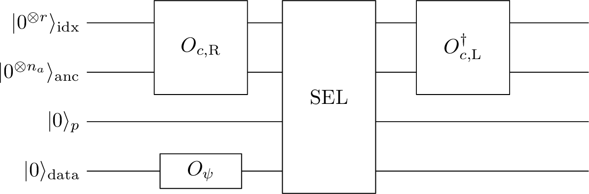
For clarity, we focus on the homogeneous case and present the overall quantum circuit that implements the corresponding LCU construction (see Fig. 1). The circuit starts from \(| 0^{\otimes r} \rangle_{\mathrm{idx}} | 0^{\otimes n_a} \rangle_{\mathrm{anc}} | 0 \rangle_{p} | 0 \rangle_{\mathrm{data}},\) where \(r=\lceil \log_2 M\rceil\). The data register is initialized by the state-preparation oracle \(O_{\psi}\) so that \(O_{\psi}| \boldsymbol{0} \rangle_{\mathrm{data}}=| \boldsymbol{u}_0 \rangle_{\mathrm{data}},\) while the position qubit remains in the state \(| 0 \rangle_{p}\). Equivalently, the joint \(p\)–data register is initialized as \(| \boldsymbol{\psi}_0 \rangle = | 0 \rangle_{p}| \boldsymbol{u}_0 \rangle_{\mathrm{data}}.\) The ancilla register in Fig. 1 represents the collection of auxiliary qubits used by the coefficient-preparation oracles and by \(\mathrm{SEL}\).
4.4 Query complexity↩︎
Let \(\Pi_h:=\langle 0 |_p\otimes I_N\). Since \(\boldsymbol{u}_f^a\) in 36 –37 already denotes the all-zero index–ancilla branch on the joint \(p\)-data register, the implemented physical branch is \(\boldsymbol{u}_h^a:=\Pi_h\boldsymbol{u}_f^a\). The target physical solution is \(\boldsymbol{u}_h(T):=\Pi_h\boldsymbol{u}_f^{\mathrm{disc}}(T)\), with \(\boldsymbol{u}_f^{\mathrm{disc}}(T)\) defined in 17 .
The circuit \(V_0\) prepares the unnormalized augmented vector \(\boldsymbol{u}_f^a\) with prefactor \(1/\eta_0\). Thus the joint success probability for obtaining the physical branch is \(\|\boldsymbol{u}_h^a\|^2/\eta_0^2\). In the proof below, the implementation errors are chosen so that \(\|\boldsymbol{u}_h^a-\boldsymbol{u}_h(T)\|=O(\varepsilon\|\boldsymbol{u}_h(T)\|)\), and hence \(\|\boldsymbol{u}_h^a\|=\Theta(\|\boldsymbol{u}_h(T)\|)\). Applying oblivious amplitude amplification, the repetition factor satisfies \[\label{eq:repeat-times-new} g = O\!\left(\frac{\eta_0}{\|\boldsymbol{u}_h^a\|}\right) = O\!\left(\frac{\eta_0}{\|\boldsymbol{u}_h(T)\|}\right) = O\!\left( \frac{\alpha_c\|\boldsymbol{u}_0\|+\alpha_d\|\boldsymbol{b}\|}{\|\boldsymbol{u}_h(T)\|} \right).\tag{38}\] Define \[\label{eq:vr-def-new} u_r := \frac{\|\boldsymbol{u}_0\|+ T\|\boldsymbol{b}\|}{\|\boldsymbol{u}_h(T)\|}.\tag{39}\] The resulting query complexity bounds are stated in Theorem 2.
Theorem 2. Consider the linear equation in 3 with \(\mathcal{A}=\mathcal{L}^{\dagger}\mathcal{L}\) self-adjoint. Let \(L\) be the matrix obtained from the spatial discretization of \(\mathcal{L}\). There exists a quantum algorithm that prepares an \(\varepsilon\)-approximation of the normalized solution state \(| \boldsymbol{u}_h(T) \rangle\) with \(\Omega(1)\) success probability and a success flag. Moreover, the total query complexity to the block-encoding oracle for \(L\) is \[\widetilde{O}\!\left( u_r\Bigl( \|L\|\sqrt{T\,\log\!\frac{u_r}{\varepsilon}} + \log\!\frac{u_r}{\varepsilon} \Bigr) \right),\] and the number of calls to the state-preparation oracles \(O_{\psi}\) and \(O_b\) is \(O(u_r)\).
The above guarantees hold under the following default choices of auxiliary parameters.
Table . Default discretization choices used in the proof.
| Parameter | Meaning | Default choice |
|---|---|---|
| \(R\) | truncation radius in \(s\) | \(R = 2\sqrt{T\,\log\!\bigl(\dfrac{8u_r}{\varepsilon}\bigr)}\) |
| \(h_1\) | panel length in \(s\) (step size) | \(h_1 = \dfrac{1}{e\bigl(\|L\|+1/\sqrt{2T}\bigr)}\) |
| \(Q\) | reference Gauss points per panel | \(Q = O\!\bigl(\log\!\bigl(\dfrac{8u_r}{\varepsilon}\bigr)\bigr)\) |
| \(\delta_{\mathrm{off}}\) | offline approximation error in 20 | \(\delta_{\mathrm{off}} = \dfrac{\varepsilon}{32u_r}\) |
Proof. Let \(\boldsymbol{u}_f^{\mathrm{disc}}\) be the exact semi-discrete Kannai target in 17 , let \(\boldsymbol{u}_f^{h}\) be the corresponding truncated quadrature target in 21 , and let \(\boldsymbol{u}_f^{a}\) be the unnormalized vector produced by the quantum circuit in 37 . Since \(\Pi_h\) is a contraction, the augmented-vector errors imply \[\|\boldsymbol{u}_h^a-\boldsymbol{u}_h(T)\| \le \|\boldsymbol{u}_f^a-\boldsymbol{u}_f^h(T)\| + \|\boldsymbol{u}_f^h(T)-\boldsymbol{u}_f^{\mathrm{disc}}(T)\|.\] For any nonzero vectors \(\boldsymbol{x}\) and \(\boldsymbol{y}\), \[\left\| \frac{\boldsymbol{x}}{\|\boldsymbol{x}\|} - \frac{\boldsymbol{y}}{\|\boldsymbol{y}\|} \right\| \le \frac{2\|\boldsymbol{x}-\boldsymbol{y}\|}{\|\boldsymbol{x}\|}.\] Applying this with \(\boldsymbol{x}=\boldsymbol{u}_h(T)\) and \(\boldsymbol{y}=\boldsymbol{u}_h^a\) yields \[\label{eq:total-error-split-new} \left\| | \boldsymbol{u}_h^a \rangle - | \boldsymbol{u}_h(T) \rangle \right\| \le \frac{2\|\boldsymbol{u}_f^{\mathrm{disc}}(T)-\boldsymbol{u}_f^h(T)\|}{\|\boldsymbol{u}_h(T)\|} + \frac{2\|\boldsymbol{u}_f^h(T)-\boldsymbol{u}_f^a\|}{\|\boldsymbol{u}_h(T)\|}.\tag{40}\]
4.4.0.1 Step 1: Discretization error
Choose the discretization parameters \((R,h_1,Q,\delta_{\mathrm{off}})\) as in Table [tab:disc-params], obtained by applying Theorem 1 with target accuracy \(\varepsilon/(8u_r)\). Then \[\|\boldsymbol{u}_f^{\mathrm{disc}}(T)-\boldsymbol{u}_f^h(T)\| \le \frac{\varepsilon}{8u_r} \bigl(\|\boldsymbol{u}_0\|+T\|\boldsymbol{b}\|\bigr) = \frac{\varepsilon}{8}\|\boldsymbol{u}_h(T)\|.\] Thus the first term in 40 is at most \(\varepsilon/4\).
4.4.0.2 Step 2: Error from imperfect implementation of unitaries
Let \(U(s)=e^{-iHs}\) and let \(U_j^a\) be the unitaries implemented by the selector \(\mathrm{SEL}\), satisfying \(\|U_j^a-U(s_j)\|\le \delta_1\) for all \(j\) as in 31 . Using the LCU representations of \(\boldsymbol{u}_f^{h}\) and \(\boldsymbol{u}_f^{a}\) yields \[\begin{align} \label{eq:HS-LCU-error-new} \|\boldsymbol{u}_f^{h}-\boldsymbol{u}_f^{a}\| = \big\| \sum_{j=0}^{M-1} c_j\bigl(U(s_j)-U_j^a\bigr)\boldsymbol{\psi}_0 + \sum_{j=0}^{M-1} d_j\bigl(U(s_j)-U_j^a\bigr)\boldsymbol{b}\big \| = O\!\left(\delta_1 u_r\|\boldsymbol{u}_h(T)\|\right). \end{align}\tag{41}\] Choosing \(\delta_1=\Theta(\varepsilon/u_r)\) makes the second term in 40 at most \(\varepsilon/4\).
Combining the two steps gives \[\left\| | \boldsymbol{u}_h^a \rangle - | \boldsymbol{u}_h(T) \rangle \right\| \le \frac{\varepsilon}{2},\] hence in particular an \(\varepsilon\)-approximation of the normalized physical solution state.
4.4.0.3 Step 3: Query complexity
Each invocation of \(\mathrm{SEL}\) uses \[\widetilde{O}\!\left(\alpha_H s_{\max}+\log\frac{1}{\delta_1}\right) = \widetilde{O}\!\left(\|L\|\,R+\log\frac{u_r}{\varepsilon}\right)\] queries to the block-encoding of \(H\), by 32 and the choice \(\delta_1=\Theta(\varepsilon/u_r)\). Since the block-encoding of \(H\) is constructed from the block-encoding of \(L\) using only \(O(1)\) calls to \(L\) and \(L^\dagger\), we count this as the same order of queries to the block-encoding oracle for \(L\). With the parameter choices in Table [tab:disc-params], one has \(R=\Theta\bigl(\sqrt{T\log(u_r/\varepsilon)}\bigr)\). Postselecting the position qubit yields a state proportional to \(\boldsymbol{u}_h^a\), which has been shown above to give an \(\varepsilon\)-approximation of \(| \boldsymbol{u}_h(T) \rangle\) after normalization. The repetition factor is \(g=O(u_r)\) by 38 . The number of calls to \(O_{\psi}\) and \(O_b\) is also \(O(u_r)\) since each attempt invokes them \(O(1)\) times. ◻
Remark 2. Theorem 2 yields only polylogarithmic dependence on the target accuracy \(\varepsilon\). Many quantum constructions for non-unitary linear dynamics approximate the propagator denoted by \(\mathcal{S}(T,0)\) via a truncated unitary superposition \[\mathcal{S}(T,0)u_0 \approx \int_{-R}^{R} K(s)\,e^{-iHs}u_0\,\mathrm{d}s, \qquad 2\int_R^\infty |K(s)|\,\mathrm{d}s \le \varepsilon,\] for which the dominant matrix-query cost is typically proportional to \(R\) up to polylogarithmic factors. In our case, the Kannai kernel is Gaussian, giving \[R=\Theta \bigl(\sqrt{T\log(1/\varepsilon)}\bigr),\] and hence the dominant term in the query bound is \(\widetilde{O}\!\bigl(u_r\,\|L\|\sqrt{T\log(1/\varepsilon)}\bigr)\). Moreover, since \(A=L^\dagger L\), we have \(\|L\|=\|A\|^{1/2}\), so the bound exhibits a square-root dependence on \(\|A\|\) rather than a linear one, improving upon [21], [43], [44]. Fig. 2 illustrates the truncation behavior of the corresponding kernels. In particular, our improved dependence can be summarized as \[\widetilde{O}\bigl(\sqrt{\alpha_A T\log(1/\varepsilon)}\bigr),\] as reported in Table 1 for the homogeneous setting.
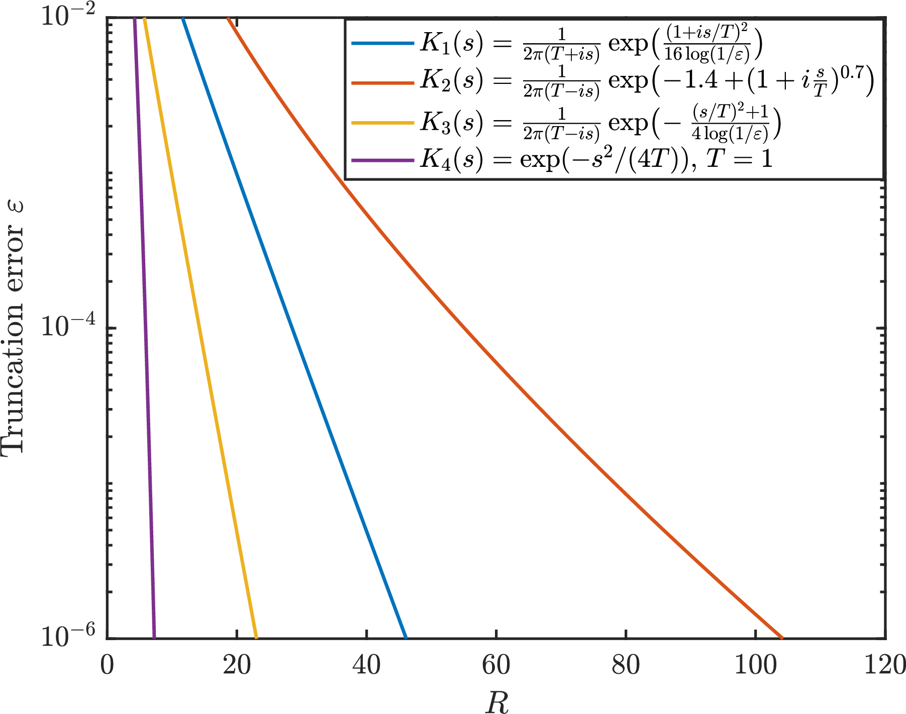
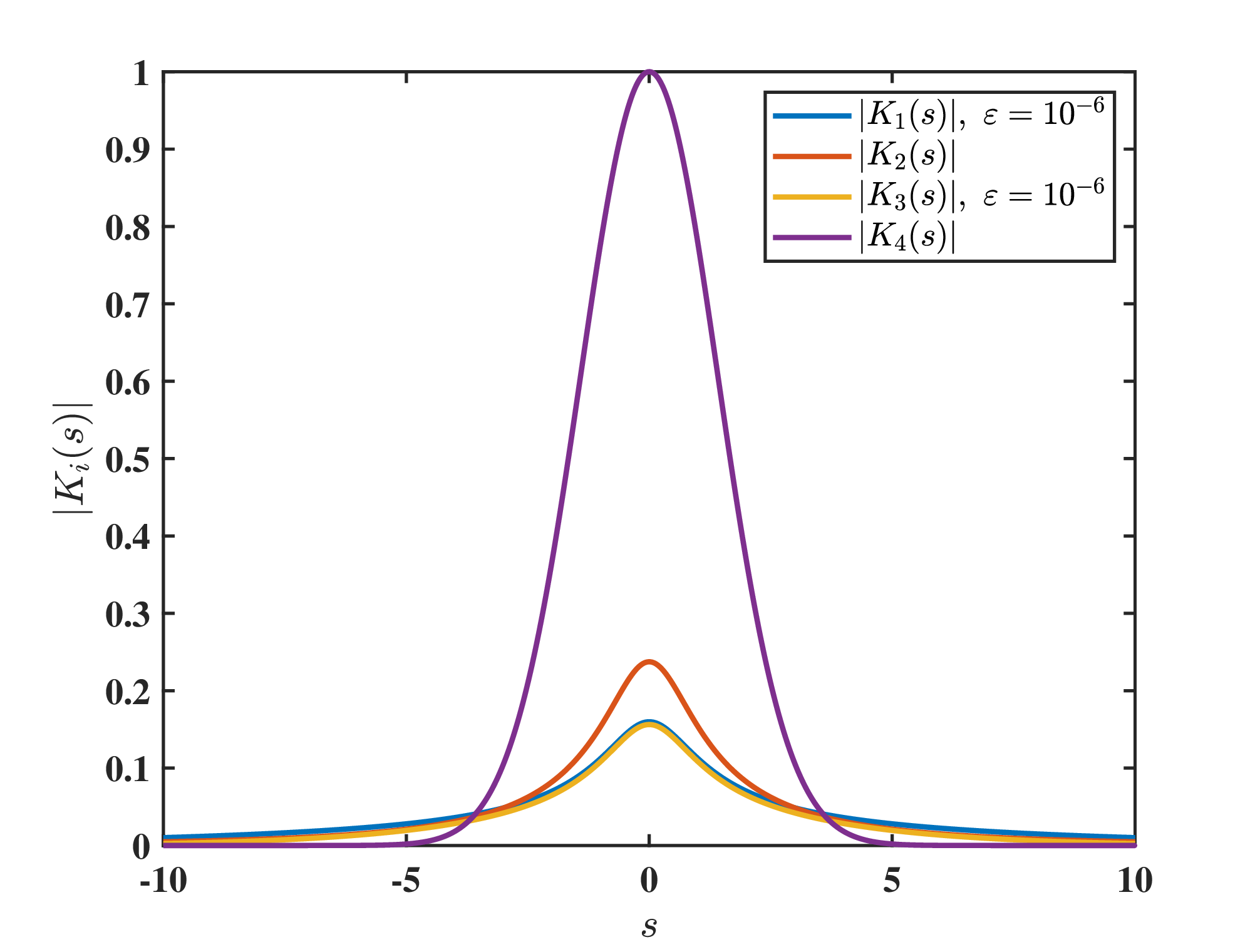
Figure 2: Kernel truncation behavior for several unitary-superposition representations. Left: truncation error \(\varepsilon(R):=2\int_{R}^{\infty}\!\lvert K_i(s)\rvert\,\mathrm{d}s\) as a function of the truncation length \(R\) (logarithmic scale in \(\varepsilon\)). Right: kernel magnitudes \(\lvert K_i(s)\rvert\) on \(s\in[-10,10]\) for a fixed target precision \(\varepsilon=10^{-6}\) and \(T=1\)..
| Method | Kernel \(K(s)\) | Truncation length | Matrix queries |
|---|---|---|---|
| Schrödingerization | \(\vspace{1mm} \displaystyle \frac{e^{\frac{(1+is^2/T^2)}{16\log(1/\varepsilon)}}}{2\pi (T +i s)} \vspace{1mm}\) | \(\displaystyle O\!\bigl(T\log\frac{1}{\varepsilon}\bigr)\) | \(\displaystyle \widetilde{O}\!\big( u_r\, \alpha_A\,T\,\log\frac{1}{\varepsilon} \big)\) |
| \(\vspace{1mm} \displaystyle \frac{e^{2^{\beta}-(1+i \frac{s}{T})^{\beta}}}{2\pi(T-i s)} \vspace{1mm}\) | \(\displaystyle O\!\bigl(T\log^{\frac{1}{\beta}}\frac{1}{\varepsilon}\bigr)\) | \(\displaystyle \widetilde{O}\!\big( u_r\, \alpha_A\,T\,\log^{\frac{1}{\beta}}\frac{1}{\varepsilon} \big)\) | |
| \(\vspace{1mm} \displaystyle \frac{e^{-\frac{1+ s^2/T^2}{4\log(1/\varepsilon)}}}{2\pi(T-i s)} \vspace{1mm}\) | \(\displaystyle O\!\bigl(T\log\frac{1}{\varepsilon}\bigr)\) | \(\displaystyle \widetilde{O}\!\big( u_r\, \alpha_A\,T\,\log\frac{1}{\varepsilon} \big)\) | |
| This work | \(\vspace{1mm} \displaystyle \frac{e^{-\frac{s^2}{4T}}}{\sqrt{4\pi T}} \vspace{1mm}\) | \(\displaystyle O\!\big(\sqrt{T\log\frac{1}{\varepsilon}}\big)\) | \(\displaystyle \widetilde{O}\!\big( u_r\, \sqrt{\alpha_A\,T\,\log\frac{1}{\varepsilon}} \big)\) |
4.5 Extension beyond the factorized generator \(A=L^\dagger L\)↩︎
In this subsection we extend the framework to time-independent generators \(A\in\mathbb{C}^{N\times N}\) that are not necessarily of the form \(L^\dagger L\). For clarity, we focus on the homogeneous system \[\label{eq:hom95generalA} \frac{\mathrm{d}}{\mathrm{d}t}\boldsymbol{u}(t)=-A\,\boldsymbol{u}(t),\qquad \boldsymbol{u}(0)=\boldsymbol{u}_0,\tag{42}\] since the inhomogeneous case can be handled analogously via Duhamel’s principle. Throughout this subsection we omit auxiliary workspace qubits used by reversible arithmetic and Hamiltonian simulation, as they are uncomputed at the end. We use the Cartesian decomposition \[\label{eq:cartesian95decomp} A = H_1 + iH_2, \qquad H_1:=\frac{A+A^\dagger}{2}, \qquad H_2:=\frac{A-A^\dagger}{2i},\tag{43}\] where \(H_1\) and \(H_2\) are Hermitian. Assuming \(H_1\succeq 0\), we may factor \[\label{eq:H195factorization} H_1=L^\dagger L\tag{44}\] for some matrix \(L\).
4.5.1 Normal case \(AA^{\dagger} = A^{\dagger} A\)↩︎
If \(A\) is normal, then \([H_1,H_2]=0\) and the propagator factors as \[\label{eq:factorization95commuting} \boldsymbol{u}(T)=e^{-AT}\boldsymbol{u}_0 = e^{-H_1T}\,e^{-iH_2T}\,\boldsymbol{u}_0 = e^{-L^\dagger L\,T}\,e^{-iH_2T}\,\boldsymbol{u}_0.\tag{45}\] We therefore first implement the unitary \(e^{-iH_2T}\) by Hamiltonian simulation and then apply the dissipative factor \(e^{-L^\dagger L\,T}\) using the Kannai-transform LCU routine.
Let \(H\) be the Hermitian dilation associated with \(L\) as in 13 and define \(U(s)=e^{-iHs}\). Set \[\label{eq:kannai95commuting320} U_{\kappa_T}:=\int_{\mathbb{R}}\kappa_T(s)\,U(s)\,\mathrm{d}s, \qquad \kappa_T(s)=(4\pi T)^{-1/2}e^{-s^2/(4T)}.\tag{46}\] After truncation and quadrature, \(U_{\kappa_T}\) is realized by an LCU unitary \(U_{\mathrm{LCU},T}\). Let \(n_a\) denote the number of ancilla qubits used by this LCU block.
Let the position qubit \(p\) encode the \(2\times 2\) block structure and initialize \(| \boldsymbol{\psi}_0 \rangle:=| 0 \rangle_p| \boldsymbol{u}_0 \rangle_{\mathrm{data}}\). Then the Kannai representation reads \[\label{eq:kannai95commuting} e^{-L^\dagger L\,T}| \boldsymbol{u}_0 \rangle = (\langle 0 |_p\otimes I)\,U_{\kappa_T}\,| \boldsymbol{\psi}_0 \rangle.\tag{47}\] Combining 45 and 47 , we obtain \[\label{eq:final95commuting95formula} | \boldsymbol{u}(T) \rangle \;\approx\; (\langle 0^{\otimes r} |_{\mathrm{idx}}\langle 0^{\otimes n_a} |_{\mathrm{anc}}\langle 0 |_{p}\otimes I)\, U_{\mathrm{LCU},T}\, | 0^{\otimes r} \rangle_{\mathrm{idx}}| 0^{\otimes n_a} \rangle_{\mathrm{anc}}| 0 \rangle_{p}\, \bigl(e^{-iH_2T}| \boldsymbol{u}_0 \rangle_{\mathrm{data}}\bigr).\tag{48}\] The query complexity is summarized in Corollary 1.
Corollary 1. Let \(A\in\mathbb{C}^{N\times N}\) satisfy the decomposition 43 with \(H_1\succeq 0\) and factorization \(H_1=L^\dagger L\) as in 44 , and assume \([H_1,H_2] = 0\). Assume (i) block-encoding access to \(L\) as in 24 , and (ii) Hamiltonian-simulation access to \(H_2\), e.g., via an \((\alpha_{H_2},a,0)\) block-encoding oracle. Then the state \(| \boldsymbol{u}(T) \rangle\propto e^{-AT}| \boldsymbol{u}_0 \rangle\) can be prepared using 48 up to accuracy \(\varepsilon\), with total query complexity \[\widetilde{O}\!\left( u_r\Bigl( \|L\|\sqrt{T\,\log\!\frac{u_r}{\varepsilon}} +\log\!\frac{u_r}{\varepsilon} +\alpha_{H_2}T \Bigr) \right), \qquad u_r := \frac{\|\boldsymbol{u}_0\|}{\|\boldsymbol{u}(T)\|},\] up to polylogarithmic factors. Moreover, the number of calls to the state-preparation oracles is \(O(u_r)\).
4.5.2 Non-normal case \(AA^\dagger\neq A^\dagger A\)↩︎
In this case, equivalently \([H_1,H_2]\neq0\), the factorization \(e^{-(H_1+iH_2)T}=e^{-H_1T}e^{-iH_2T}\) is no longer available. Let \(\tau=T/N_t\). We use the Strang splitting–which has second-order accuracy: \[\label{eq:strang95noncommute} e^{-(H_1+iH_2)T} \approx \left(e^{-iH_2\tau/2}e^{-H_1\tau}e^{-iH_2\tau/2}\right)^{N_t}.\tag{49}\]
Let \(H\) be the Hermitian dilation associated with \(L\) as in 13 , and set \(U(s)=e^{-iHs}\). For one step of length \(\tau\), define \[U_{\kappa_\tau} := \int_{\mathbb{R}}\kappa_\tau(s)U(s)\,\mathrm ds, \qquad \kappa_\tau(s)=(4\pi\tau)^{-1/2}e^{-s^2/(4\tau)} .\] By the Kannai block identity 47 , with \(T\) replaced by \(\tau\) and \(L^\dagger L=H_1\), it holds \[\label{eq:kannai95block95tau} E_\tau := (\langle 0 |_p\otimes I)U_{\kappa_\tau}(| 0 \rangle_p\otimes I) = e^{-H_1\tau}.\tag{50}\]
Let \(\{s_\ell(\tau),c_\ell(\tau)\}_{\ell=0}^{M-1}\) be the quadrature nodes and LCU coefficients for the one-step kernel \(\kappa_\tau\), and let \(U_\ell^a\) be the Hamiltonian-simulation approximation of \(U(s_\ell(\tau))=e^{-iH s_\ell(\tau)}\). Set \[\label{eq:U95kappa95tau95lcu0} \widetilde{U}_{\kappa_\tau} := \sum_{\ell=0}^{M-1}c_\ell(\tau)U_\ell^a, \qquad \alpha_c(\tau):=\sum_{\ell=0}^{M-1}|c_\ell(\tau)|.\tag{51}\] Its physical dissipative block is \[\widetilde{E}_\tau := (\langle 0 |_p\otimes I)\widetilde{U}_{\kappa_\tau}(| 0 \rangle_p\otimes I) \approx e^{-H_1\tau}.\] Set \[V_\tau:=I_p\otimes e^{-iH_2\tau/2}, \qquad \widetilde{\mathcal{T}}_\tau := V_\tau\widetilde{U}_{\kappa_\tau}V_\tau .\] Here \(\widetilde{\mathcal{T}}_\tau\) acts on the enlarged space \(\mathcal{H}_p\otimes\mathcal{H}_{\rm data}\). Its one-step physical block on the data space is \[\label{eq:S95tau95physical} \widetilde{\mathscr{T}}_\tau := (\langle 0 |_p\otimes I)\widetilde{\mathcal{T}}_\tau(| 0 \rangle_p\otimes I) = e^{-iH_2\tau/2}\widetilde{E}_\tau e^{-iH_2\tau/2}.\tag{52}\]
We do not postselect after each step. Instead, we use a single global LCU for the entire product. Since \[\widetilde{\mathcal{T}}_\tau = \sum_{\ell=0}^{M-1}c_\ell(\tau)V_\tau U_\ell^aV_\tau,\] expanding the \(N_t\)-fold product gives \[\label{eq:global95path95expansion} (\widetilde{\mathcal{T}}_\tau)^{N_t} = \sum_{\boldsymbol{\ell}\in\{0,\ldots,M-1\}^{N_t}} c_{\boldsymbol{\ell}}(\tau)\,\mathcal{U}_{\boldsymbol{\ell}},\tag{53}\] where \(\boldsymbol{\ell}=(\ell_1,\ldots,\ell_{N_t})\), \(c_{\boldsymbol{\ell}}(\tau):=\prod_{k=1}^{N_t}c_{\ell_k}(\tau)\) , and \(\mathcal{U}_{\boldsymbol{\ell}} := (V_\tau U_{\ell_{N_t}}^aV_\tau)\cdots(V_\tau U_{\ell_1}^aV_\tau)\). The order of these factors is kept fixed, since the operators do not need to commute.
Let \(U_{\rm path}\) be the corresponding path-LCU unitary. Then \[\label{eq:path95block95full} (\langle \mathbf{0} |_{\rm path}\otimes I_{p,{\rm data}}) U_{\rm path} (| \mathbf{0} \rangle_{\rm path}\otimes I_{p,{\rm data}}) = \frac{(\widetilde{\mathcal{T}}_\tau)^{N_t}}{\alpha_{\rm path}},\tag{54}\] with \[\alpha_{\rm path} := \sum_{\boldsymbol{\ell}}|c_{\boldsymbol{\ell}}(\tau)| = \alpha_c(\tau)^{N_t}.\] Applying the coefficient bound in Theorem 1 to the one-step kernel \(\kappa_\tau\), with target accuracy \(O(\varepsilon/(u_rN_t))\), gives \[\alpha_c(\tau) \le 1+O\!\left(\frac{\varepsilon}{u_rN_t}\right).\] Consequently, \[\alpha_{\rm path} = \alpha_c(\tau)^{N_t} = O(1).\] Hence the LCU normalization does not introduce an exponential loss in \(N_t\).
The operator induced on the physical data space by the full path construction is \[\label{eq:S95path95def} \widetilde{\mathcal{T}}_{\rm path}(T) := (\langle 0 |_p\otimes I)(\widetilde{\mathcal{T}}_\tau)^{N_t}(| 0 \rangle_p\otimes I).\tag{55}\] Consequently, \[\label{eq:path95block95noncommute} (\langle \mathbf{0} |_{\rm path}\langle 0 |_p\otimes I) U_{\rm path} (| \mathbf{0} \rangle_{\rm path}| 0 \rangle_p\otimes I) = \frac{\widetilde{\mathcal{T}}_{\rm path}(T)}{\alpha_{\rm path}}.\tag{56}\] If the symmetric quadrature and Hamiltonian-simulation subroutines preserve the \(p=0\) subspace exactly, then \(\widetilde{\mathcal{T}}_{\rm path}(T)=\widetilde{\mathscr T}_{\tau}^{N_t}\); otherwise the possible leakage is included in the step implementation error. For a normalized input, the success probability is \[p_{\rm succ} = \frac{\|\widetilde{\mathcal{T}}_{\rm path}(T)\boldsymbol{u}_0\|^2}{\alpha_{\rm path}^2\|\boldsymbol{u}_0\|^2},\] so the final amplitude-amplification overhead is governed by the output-norm factor \(u_r\), not by an exponential factor in \(N_t\). The normalized output is \[\label{eq:final95noncommuting95formula} | \boldsymbol{u}(T) \rangle \approx \frac{ (\langle \mathbf{0} |_{\rm path}\langle 0 |_p\otimes I) U_{\rm path}| \mathbf{0} \rangle_{\rm path}| 0 \rangle_p| \boldsymbol{u}_0 \rangle }{ \left\| (\langle \mathbf{0} |_{\rm path}\langle 0 |_p\otimes I) U_{\rm path}| \mathbf{0} \rangle_{\rm path}| 0 \rangle_p| \boldsymbol{u}_0 \rangle \right\| }.\tag{57}\]
Corollary 2. Let \(A\in\mathbb{C}^{N\times N}\) admit the decomposition 43 with \(H_1\succeq0\) and factorization \(H_1=L^\dagger L\) as in 44 , and assume \([H_1,H_2]\neq0\). Define \[\Lambda := \|[H_2,[H_2,H_1]]\| + \|[H_1,[H_1,H_2]]\| .\] For any \(T>0\) and normalized-state accuracy \(\varepsilon\in(0,1)\), choose \[N_t = \Theta\!\left(\sqrt{\frac{\Lambda T^3u_r}{\varepsilon}}\right), \qquad u_r:=\frac{\|\boldsymbol{u}_0\|}{\|\boldsymbol{u}(T)\|}.\] Assume block-encoding access to \(L\) as in 24 and Hamiltonian-simulation access to \(H_2\), for instance via an \((\alpha_{H_2},a,0)\) block-encoding oracle. Then the state \(| \boldsymbol{u}(T) \rangle\propto e^{-AT}| \boldsymbol{u}_0 \rangle\) can be prepared using 57 up to accuracy \(\varepsilon\) with query complexity \[\widetilde{O}\!\left( u_r\left( \|L\|\left(\frac{\Lambda T^5u_r}{\varepsilon}\right)^{1/4} + \sqrt{\frac{\Lambda T^3u_r}{\varepsilon}} \log\frac{u_rN_t}{\varepsilon} + \alpha_{H_2}T \right) \right).\] Moreover, the number of calls to the state-preparation oracle is \(O(u_r)\).
Proof. The Strang splitting error satisfies \[\left\| e^{-(H_1+iH_2)T} - \left(e^{-iH_2\tau/2}e^{-H_1\tau}e^{-iH_2\tau/2}\right)^{N_t} \right\| = O(\Lambda T\tau^2).\] For normalized states, it is enough to make the operator error \(O(\varepsilon/u_r)\), using the standard inequality \[\left\|\frac{\boldsymbol{x}}{\|\boldsymbol{x}\|}-\frac{\boldsymbol{y}}{\|\boldsymbol{y}\|}\right\| \le \frac{2\|\boldsymbol{x}-\boldsymbol{y}\|}{\|\boldsymbol{x}\|}.\] This gives the stated choice of \(N_t\).
For each step, the Kannai LCU approximates \(e^{-H_1\tau}\) in the physical block. The quadrature, Hamiltonian-simulation, and block-leakage errors are chosen at level \(O(\varepsilon/(u_rN_t))\), so that their accumulated contribution is \(O(\varepsilon/u_r)\). The same choice gives \(\alpha_{\rm path}=\alpha_c(\tau)^{N_t}=O(1)\), hence the final success probability is \(\Omega(1/u_r^2)\) and amplitude amplification contributes a factor \(O(u_r)\).
One path-SELECT applies \(N_t\) controlled one-step Kannai simulations. The total Kannai cost per attempt is therefore \[\widetilde{O}\!\left( N_t\left(\|L\|\sqrt\tau+ \log\frac{u_rN_t}{\varepsilon}\right) \right) = \widetilde{O}\!\left( \|L\|\left(\frac{\Lambda T^5u_r}{\varepsilon}\right)^{1/4} + \sqrt{\frac{\Lambda T^3u_r}{\varepsilon}} \log\frac{u_rN_t}{\varepsilon} \right).\] The two \(H_2\) half steps over all Strang steps have total simulated time \(T\), giving an additional \(\widetilde{O}(\alpha_{H_2}T)\) cost. Multiplication by the final amplification factor \(O(u_r)\) yields the claimed complexity. ◻
Remark 3. If \([H_1,H_2]=0\) and \(H_1=L^\dagger L\), the commuting construction of Corollary 1 applies. If \([H_1,H_2]\neq0\), the above global path LCU combines the same Kannai block for \(e^{-H_1\tau}\) with Strang’s splitting, while avoiding intermediate measurements.
5 Complexity for representative PDEs↩︎
In this section, we instantiate the general complexity bound in Theorem 2 for representative partial differential equations. We focus on how boundary conditions and spatial discretization determine the operator norm \(\|L\|\), and hence the overall query complexity of the proposed quantum algorithm.
5.1 The heat equation↩︎
We begin with the heat equation on a bounded domain \(\Omega\subset\mathbb{R}^d\), \[\partial_t u = -\mathcal{A}u + f, \qquad \mathcal{L}=-\nabla, \qquad \mathcal{L}^{\dagger}=\mathrm{div}, \qquad u(0,x)=u_0(x),\] so that \(\mathcal{A}=\mathcal{L}^\dagger\mathcal{L}=-\mathrm{div}\,\nabla\). Consider Dirichlet boundary data \[u(t,x)\big|_{x\in\partial\Omega} = u_d(x), \qquad t\ge 0.\] In the first-order embedding \(\boldsymbol{\psi}=[\,w\;\;v\,]^\top\), the boundary condition is imposed on the auxiliary variable \(w\) by requiring \[w(s,x)\big|_{x\in\partial\Omega}=u_d(x), \qquad \text{for all } s.\] Since the reconstruction uses the projection \(\Pi_1\boldsymbol{\psi}=w\), the recovered solution \(u(t,\cdot)\) inherits the prescribed Dirichlet values.
We discretize the first-order system for \(\boldsymbol{\psi}=[\,w\;\;v\,]^\top\) on a staggered grid such that the discrete gradient and divergence are represented by \(-L\) and \(L^\dagger\), respectively.
In one dimension, let \(\Omega=(0,1)\) and \(h=1/N_x\). Place \(w\) on primary nodes \(x_i=ih\) and \(v\) on midpoints \(x_{i+\frac{1}{2}}=(i+\tfrac12)h\). Collect \[\begin{align} \boldsymbol{w}_h(s)&=(w_1(s),\ldots,w_{N_x-1}(s))^\top\in\mathbb{R}^{N_x-1},\\ \boldsymbol{v}_h(s)&=(v_{1/2}(s),\ldots,v_{N_x-1/2}(s))^\top\in\mathbb{R}^{N_x}, \end{align}\] and enforce Dirichlet data by fixing \(w_0(s)=u_d(x_0)\) and \(w_{N_x}(s)=u_d(x_{N_x})\) for all \(s\). Define the interior difference operator \(D_h\in\mathbb{R}^{N_x\times(N_x-1)}\) by \[\label{eq:L-1D} (D_h\boldsymbol{w}_h)_{i+\frac{1}{2}} := \begin{cases} -\dfrac{w_1}{h}, & i=0,\\[0.7em] -\dfrac{w_{i+1}-w_i}{h}, & i=1,\ldots,N_x-2,\\[0.7em] \dfrac{w_{N_x-1}}{h}, & i=N_x-1 . \end{cases}\tag{58}\] For nonhomogeneous Dirichlet data, the boundary values \(w_0(s)=u_d(x_0)\) and \(w_{N_x}(s)=u_d(x_{N_x})\) are treated as boundary lifting terms. Equivalently, \[-\frac{w_{i+1}-w_i}{h} = (D_h\boldsymbol{w}_h)_{i+\frac{1}{2}} + (\boldsymbol{f}_{\rm bd}^{(1)})_{i+\frac{1}{2}},\] where \[\boldsymbol{f}_{\rm bd}^{(1)} = \frac{1}{h} \bigl( u_d(x_0),0,\ldots,0,-u_d(x_{N_x}) \bigr)^\top \in\mathbb{R}^{N_x}.\] The vector \(\boldsymbol{f}_{\rm bd}^{(1)}\) is absorbed into the inhomogeneous source term. In particular, for homogeneous Dirichlet data, \(\boldsymbol{f}_{\rm bd}^{(1)}=0\). Then \[(\nabla w)_{i+\frac{1}{2}} \approx -(D_h\boldsymbol{w}_h+\boldsymbol{f}_{\rm bd}^{(1)})_{i+\frac{1}{2}}, \qquad (\operatorname{div} v)_i \approx (D_h^\top \boldsymbol{v}_h)_i .\] We write \(L:=D_h\) for the interior difference operator in one dimension.
In \(d\) dimensions on \(\Omega=(0,1)^d\), order interior nodal values of \(w\) into \(\boldsymbol{w}_h(s)\in\mathbb{R}^{M_w}\) with \(M_w=(N_x-1)^d\), and collect staggered face values of \(v\) into \(\boldsymbol{v}_h(s)\in\mathbb{R}^{M_v}\). For nonhomogeneous Dirichlet data, the tensor-product lifting of \(\boldsymbol{f}_{\rm bd}^{(1)}\) in each coordinate direction is absorbed into the source vector. Thus the operator \(L\) below acts only on the interior nodal unknowns. Lift \(D_h\) to each coordinate direction by \[\label{eq:Lk-kron} L^{(k)}= I_{N_x-1}^{\otimes (k-1)}\otimes D_h\otimes I_{N_x-1}^{\otimes (d-k)}, \qquad k=1,\ldots,d,\tag{59}\] and stack the directional operators as \[L= \begin{bmatrix} (L^{(1)})^{\dagger} & (L^{(2)})^{\dagger} & \cdots & (L^{(d)})^{\dagger} \end{bmatrix}^{\dagger}.\] Then \(L:\mathbb{R}^{M_w}\to\mathbb{R}^{M_v}\) discretizes \(-\nabla\) on the staggered grid and \(L^\dagger\) discretizes \(\mathrm{div}\). The semi-discrete first-order system is obtained from the continuum formulation by replacing \((\mathcal{L},\mathcal{L}^\dagger)\) with \((L,L^\dagger)\).
Remark 4. For homogeneous Neumann data \(\partial_n u=0\) on \(\partial\Omega\), it is natural to impose the boundary condition on the flux component. One convenient staggered placement samples \(v\) on primary nodes and \(w\) on staggered locations, so that the normal component of \(v\) can be fixed to zero on \(\partial\Omega\). The resulting discrete gradient–divergence pair has the same structure as above, with the roles of \(w\) and \(v\) interchanged.
The following corollary specializes Theorem 2 to the heat equation under the staggered finite-difference discretization described above.
Corollary 3. Consider \(\Omega=(0,1)^d\) and the staggered finite-difference discretization above with mesh size \(h\) in each coordinate direction. Let \(L\) denote the resulting discrete gradient operator. Assume the hypotheses of Theorem 2 hold. Then there exists a quantum algorithm that prepares an \(\varepsilon\)-approximation of the normalized solution state \(| \boldsymbol{u}_h(T) \rangle\) approximating \(u\) with \(\Omega(1)\) success probability and a success flag, using \[\widetilde{O}\!\left( u_r\left( \frac{\sqrt{d}}{h}\,\sqrt{T\log\frac{u_r}{\varepsilon}} + \log\frac{u_r}{\varepsilon} \right) \right)\] queries to the block-encoding oracle for \(L\), where \[u_r= O\!\left( \frac{\|u_0\|_{L^2(\Omega)}+T\|f\|_{L^2(\Omega)}}{\|u(T)\|_{L^2(\Omega)}} \right).\] Moreover, the number of calls to the state-preparation oracles \(O_\psi\) and \(O_b\) is \(O(u_r)\).
Proof. For the staggered finite-difference discretization on \((0,1)^d\), the discrete gradient operator satisfies \(\|L\|=\Theta(\sqrt{d}/h)\). Substituting this bound into Theorem 2 yields the stated query complexity. The bound on the number of calls to \(O_\psi\) and \(O_b\) follows from the same theorem. ◻
5.2 Viscous Hamilton–Jacobi equations via entropy penalization↩︎
Hamilton–Jacobi equations are fundamental in mechanics and optimal control. Since classical solutions may develop finite-time singularities, one often passes to vanishing-viscosity regularizations and viscosity solutions. We use the entropy-penalization framework of [45], [46] only as a mechanism for producing a linear parabolic surrogate suitable for the Kannai-transform algorithm. We do not reproduce the full entropy-penalization analysis here.
For simplicity, we absorb the calibration constant in the entropy-penalization kernel into the viscosity parameter and write the effective viscosity again as \(\nu\). Thus the viscous Hamilton–Jacobi equation is written as \[\label{eq:HJ-visc} \partial_t S^\nu(t,\boldsymbol{x}) + H\!\bigl(\boldsymbol{x},\nabla S^\nu(t,\boldsymbol{x})\bigr) = \nu\,\Delta S^\nu(t,\boldsymbol{x}), \qquad S^\nu(0,\boldsymbol{x})=S_0(\boldsymbol{x}), \qquad \boldsymbol{x}\in\mathbb{T}^d .\tag{60}\]
The general entropy-penalization setting starts from a strictly convex kinetic energy \(K:\mathbb{R}^d\to\mathbb{R}\) and, possibly, a potential \(V(\boldsymbol{x})\). The corresponding Hamiltonian may be written as \[\label{eq:H-legendre} H(\boldsymbol{x},\boldsymbol{p}) = \sup_{\boldsymbol{v}\in\mathbb{R}^d} \bigl\{-\boldsymbol{p}\cdot\boldsymbol{v}-K(\boldsymbol{v})+V(\boldsymbol{x})\bigr\}.\tag{61}\]
The continuous-time limit of the entropy-penalized scheme gives a linear parabolic surrogate for an auxiliary variable \(u\) of the form [45] \[\label{eq:HJ-linear-drift-diff} \partial_t u(t,\boldsymbol{x}) = \boldsymbol{\mu}\cdot\nabla u(t,\boldsymbol{x}) + \nabla\!\cdot\!\bigl(\Sigma\nabla u(t,\boldsymbol{x})\bigr), \qquad u(0,\boldsymbol{x})=u_0(\boldsymbol{x}),\tag{62}\] where the drift vector \(\boldsymbol{\mu}\in\mathbb{R}^d\) and the diffusion matrix \(\Sigma\in\mathbb{R}^{d\times d}\) are constant in \(\boldsymbol{x}\) and \(t\). More precisely, with \[\boldsymbol{v}_\star:=\arg\min_{\boldsymbol{v}\in\mathbb{R}^d}K(\boldsymbol{v}),\] one has \[\label{eq:mu-nu-from-K} \boldsymbol{\mu}=\boldsymbol{v}_\star, \qquad \Sigma = \boldsymbol{v}_\star\boldsymbol{v}_\star^{\top} + 2\nu\bigl(\nabla^2K(\boldsymbol{v}_\star)\bigr)^{-1}.\tag{63}\]
The Cole-Hopf relation is \[\label{eq:HJ-recover} S^\nu(t,\boldsymbol{x}) = -2\nu\log u(t,\boldsymbol{x}),\tag{64}\] up to an additive normalization constant. We assume that this initial normalization is known classically; otherwise the procedure recovers \(S^\nu\) only up to an additive constant. We also assume positivity of the surrogate solution, as holds for positive Cole-Hopf initial data under the heat semigroup.
Since \(\boldsymbol{\mu}\) is constant, the drift in 62 can be removed by the translation \[\label{eq:translation} \widetilde{u}(t,\boldsymbol{x}):=u(t,\boldsymbol{x}-\boldsymbol{\mu} t).\tag{65}\] Then \(\widetilde{u}\) solves \[\label{eq:pure-diff} \partial_t\widetilde{u}(t,\boldsymbol{x}) = \nabla\!\cdot\!\bigl(\Sigma\nabla\widetilde{u}(t,\boldsymbol{x})\bigr) =:-\mathcal{A}\,\widetilde{u}(t,\boldsymbol{x}).\tag{66}\] For a nonzero drift, the value \(u(T,\boldsymbol{x}_a)\) is recovered from \(\widetilde{u}(T,\boldsymbol{x}_a+\boldsymbol{\mu} T)\) on the torus.
In the complexity estimate below, we further specialize to the isotropic constant case \[\boldsymbol{\mu}=0, \qquad \Sigma=\nu I_d,\] so that \[\mathcal{A}=-\nu\Delta .\] This is the heat-type surrogate to which we apply the general Kannai-transform state-preparation theorem.
Let \(N_x\) be the number of grid points per direction and set \(h:=1/N_x\). On the periodic grid \[\mathcal{G}_h := \{\,\boldsymbol{x}_{\boldsymbol{n}}=h\boldsymbol{n}: \boldsymbol{n}\in\{0,1,\dots,N_x-1\}^d\,\},\] we represent \(\widetilde{u}(t,\cdot)\) by the value vector \(\widetilde{\boldsymbol{u}}_h(t)\in\mathbb{C}^{N_x^d}\), defined by \[\bigl(\widetilde{\boldsymbol{u}}_h(t)\bigr)_{\boldsymbol{n}} = \widetilde{u}(t,\boldsymbol{x}_{\boldsymbol{n}}).\] Let \(U_F\) be the unitary discrete Fourier transform and define \[\widehat{\boldsymbol{u}}(t):=U_F\widetilde{\boldsymbol{u}}_h(t), \qquad \widetilde{\boldsymbol{u}}_h(t)=U_F^\dagger\widehat{\boldsymbol{u}}(t).\] We use the periodic second-order finite-difference discretization of \(-\nu\Delta\). The Fourier modes are indexed by \[\boldsymbol{k}=(k_1,\dots,k_d)\in\mathcal{K}, \qquad \mathcal{K} := \left\{ -\frac{N_x}{2},-\frac{N_x}{2}+1,\dots,\frac{N_x}{2}-1 \right\}^d , \qquad N_x\;\text{even}.\] The semi-discrete generator is diagonalised as \[\label{eq:A-diag} A=U_F^\dagger D U_F, \qquad L_{\mathrm{HJ}}:=D^{1/2}U_F, \qquad A=L_{\mathrm{HJ}}^\dagger L_{\mathrm{HJ}},\tag{67}\] where \[\label{eq:FD-symbol} D(\boldsymbol{k}) = \nu\sum_{r=1}^d \frac{4}{h^2} \sin^2\!\left(\frac{\pi k_r}{N_x}\right).\tag{68}\] Consequently, \[\label{eq:LHJ-norm} \|L_{\mathrm{HJ}}\| = \|D^{1/2}\| \le \frac{2\sqrt{d\nu}}{h}.\tag{69}\]
Applying Theorem 2 to the homogeneous semi-discrete system \[\frac{\mathrm d}{\mathrm dt}\widetilde{\boldsymbol{u}}_h(t) = -A\widetilde{\boldsymbol{u}}_h(t)\] gives the following state-preparation bound.
Corollary 4. Let \(A\) and \(L_{\mathrm{HJ}}\) be defined in 67 . There exists a quantum algorithm that prepares an \(\varepsilon\)-approximation of the normalized amplitude state \(| \widetilde{\boldsymbol{u}}_h(T) \rangle\) with \(\Omega(1)\) success probability and query complexity \[\widetilde{O}\!\left( u_r \left( \frac{\sqrt{d\nu}}{h} \sqrt{T\log\!\left(\frac{u_r}{\varepsilon}\right)} + \log\!\left(\frac{u_r}{\varepsilon}\right) \right) \right), \qquad u_r:= \frac{\|\widetilde{\boldsymbol{u}}_h(0)\|}{\|\widetilde{\boldsymbol{u}}_h(T)\|}.\]
5.2.1 Output model and accuracy for the Hamilton–Jacobi observable↩︎
Corollary 4 prepares only the normalized amplitude state of the linear parabolic surrogate. The Hamilton–Jacobi observable is obtained through the Cole-Hopf readout, not by full tomography.
Let \(\boldsymbol{u}_h(T)\) denote the unnormalized discrete vector after undoing any drift translation. In the isotropic case \(\boldsymbol{\mu}=0\), this is simply \(\boldsymbol{u}_h(T)=\widetilde{\boldsymbol{u}}_h(T)\). For a queried point \(\boldsymbol{x}_a\), let \(\boldsymbol{j}(a)\) be the corresponding grid index. If \(\boldsymbol{\mu}\neq0\), \(\boldsymbol{j}(a)\) should be replaced by the grid index corresponding to \(\boldsymbol{x}_a+\boldsymbol{\mu} T\) on the torus.
Define \[p_a := \left| \left\langle \boldsymbol{j}(a)\middle|\boldsymbol{u}_h(T)\right\rangle \right|^2, \qquad Q_a := p_a \|\boldsymbol{u}_h(T)\|^2 = \left|(\boldsymbol{u}_h(T))_{\boldsymbol{j}(a)}\right|^2 .\] Then the Cole-Hopf point-value readout is \[\label{eq:HJ-point-readout} S_{\nu,h}(T,\boldsymbol{x}_a) = -\nu\log Q_a .\tag{70}\] Thus the readout requires estimating both the point probability \(p_a\) in the normalized state and the normalization factor \(\|\boldsymbol{u}_h(T)\|^2\).
Let \[s_a:=|S_{\nu,h}(T,\boldsymbol{x}_a)|\] and assume \(s_a>0\). We require the physical point-value accuracy \[\frac{ |\widehat S_a-S(T,\boldsymbol{x}_a)| }{s_a} \lesssim \delta .\] The deterministic error has two components: the vanishing-viscosity error and the spatial discretization error. We use the model \[\label{eq:HJ-visc-error} \|S^\nu(T,\cdot)-S(T,\cdot)\|_{L^\infty} \le C_{\rm vv}D_{\rm vv}(d)\nu^\beta, \qquad \frac{1}{2}\le \beta\le 1,\tag{71}\] where \(D_{\rm vv}(d)\) records the dimension dependence of the available vanishing-viscosity estimate. In the conservative scaling used in [45], one may take \(D_{\rm vv}(d)=d\), with worst-case rate \(\beta=1/2\). For the second-order periodic finite-difference discretization above, we use the spatial error model \(O(dh^2)\). Hence it is sufficient to choose \[\label{eq:nu-h-delta-HJ} \nu = \Theta\!\left( \left( \frac{\delta s_a}{D_{\rm vv}(d)} \right)^{1/\beta} \right), \qquad h = \Theta\!\left( \sqrt{\frac{\delta s_a}{d}} \right),\tag{72}\] up to problem-dependent constants.
It remains to specify the readout accuracy. If \[\widehat Q_a=Q_a(1+\eta_Q),\] then for \(|\eta_Q|\le1/2\), \[|\widehat S_{\nu,h}(T,\boldsymbol{x}_a)-S_{\nu,h}(T,\boldsymbol{x}_a)| = \nu|\log(1+\eta_Q)| \lesssim \nu|\eta_Q|.\] Therefore an \(O(\delta)\) relative readout error in \(S_{\nu,h}(T,\boldsymbol{x}_a)\) is ensured by \[\label{eq:Q-relative-accuracy} |\eta_Q| = O\!\left( \min\left\{ \frac{1}{2},\frac{\delta s_a}{\nu} \right\} \right).\tag{73}\] The fact that the admissible relative error in \(Q_a\) can become larger when \(\nu\) is small is not a contradiction: the Cole-Hopf map multiplies the logarithmic error by \(\nu\). The difficulty for small \(\nu\) is instead reflected in the point probability \(p_a\), which may be exponentially small.
Substituting 72 into Corollary 4, and choosing the state-preparation accuracy small enough so that its induced additive error in \(p_a\) is negligible compared with \(p_a\eta_Q\), gives the matrix-query cost per successful preparation of the normalized surrogate state as \[\label{eq:HJ-delta-complexity-general} C_{\rm prep} = \widetilde{O}\!\left( u_r \left( d\,D_{\rm vv}(d)^{-\frac{1}{2\beta}} (\delta s_a)^{\frac{1}{2\beta}-\frac{1}{2}} \sqrt T + 1 \right) \right),\tag{74}\] where polylogarithmic factors in \(u_r\), \(1/\delta\), and the readout-related precision parameters are suppressed. In the conservative scaling \(D_{\rm vv}(d)=d\), this becomes \[\label{eq:HJ-delta-complexity} C_{\rm prep} = \widetilde{O}\!\left( u_r \left( d^{1-\frac{1}{2\beta}} (\delta s_a)^{\frac{1}{2\beta}-\frac{1}{2}} \sqrt T + 1 \right) \right).\tag{75}\] This is only the state-preparation cost. It is not yet the full cost of estimating \(S(T,\boldsymbol{x}_a)\), since the Cole-Hopf readout also requires estimating \(p_a\) and \(\|\boldsymbol{u}_h(T)\|^2\).
With direct sampling, the point-probability estimation requires \[N_{\rm read} = \widetilde{O}\!\left( \frac{1}{p_a\eta_Q^2} \right)\] state preparations, up to confidence logarithms and the analogous cost for estimating the normalization factor \(\|\boldsymbol{u}_h(T)\|^2\). Therefore the total direct-sampling cost scales as \[C_{\rm total} = \widetilde{O}\!\left( N_{\rm read}\,C_{\rm prep} \right).\] Amplitude estimation can improve the sampling dependence, but the readout cost remains a separate factor from the state-preparation complexity.
5.3 Biharmonic diffusion equation↩︎
We next consider the biharmonic diffusion equation \[\partial_t u = -\Delta^2 u + f,\qquad u(0,x)=u_0(\boldsymbol{x}),\qquad \boldsymbol{x}\in\Omega\subset\mathbb{R}^d.\] We impose boundary conditions so that \(\Delta^2\) is self-adjoint and nonnegative on \(L^2(\Omega)\), e.g., the simply supported plate conditions \[u=0,\qquad \Delta u=0 \quad\text{on }\partial\Omega.\] Then \(\mathcal{A}:=(-\Delta)^2=\mathcal{L}^\dagger\mathcal{L}\) with \(\mathcal{L}:=-\Delta\). In the first-order embedding \(\boldsymbol{\psi}=[\,w\;\;v\,]^\top\) in 7 –8 , we impose the homogeneous boundary conditions \[w(s,\cdot)=0,\qquad v(s,\cdot)=0 \quad\text{on }\partial\Omega .\]
We discretize \(-\Delta\) by standard second-order finite differences on a uniform grid with mesh size \(h=1/N_x\). In one dimension, collecting interior nodal values into \(\boldsymbol{w}_h(s),\boldsymbol{v}_h(s)\in\mathbb{R}^{N_x-1}\) and enforcing homogeneous Dirichlet data, we obtain \[-(\Delta w)_i \approx (D_h\boldsymbol{w}_h)_i, \qquad -(\Delta v)_i \approx ((D_h)^\top\boldsymbol{v}_h)_i, \quad i=1,\ldots,N_x-1,\] where \(D_h\) denotes the standard second-order finite-difference negative Laplacian.
In \(d\) dimensions on \(\Omega=(0,1)^d\), letting \(M_w=(N_x-1)^d\) and identifying \(\boldsymbol{w}_h(s),\boldsymbol{v}_h(s)\in\mathbb{R}^{M_w}\), we define the discrete Laplacian by the Kronecker sum \[L:=\sum_{k=1}^d \Bigl(I_{N_x-1}^{\otimes (k-1)}\otimes D_h\otimes I_{N_x-1}^{\otimes (d-k)}\Bigr),\] so that \(L\) is symmetric positive definite and approximates \(-\Delta\) with homogeneous Dirichlet data.
Corollary 5. Consider the biharmonic diffusion equation on \(\Omega=(0,1)^d\) with mesh size \(h=1/N_x\) and the discretization described above. Let \(L\) denote the discrete Laplacian. Assume that the hypotheses of Theorem 2 hold. Then there is a quantum algorithm to prepare an \(\varepsilon\)-approximation of the normalized discrete solution state \(| \boldsymbol{u}_h(T) \rangle\) with \(\Omega(1)\) success probability, using \[\widetilde{O}\!\left( u_r\left( \frac{d}{h^2}\sqrt{T\,\log\!\frac{u_r}{\varepsilon}} + \log\!\frac{u_r}{\varepsilon} \right)\right)\] queries to the block-encoding oracle for \(L\), where \[u_r= O\!\left( \frac{\|u_0\|_{L^2(\Omega)}+T\|f\|_{L^2(\Omega)}}{\|u(T)\|_{L^2(\Omega)}} \right).\] Moreover, the number of calls to the state-preparation oracles for \(\boldsymbol{\psi}_0\) and \(\boldsymbol{b}\) is \(O(u_r)\).
Proof. For the standard second-order finite-difference discretization on \(\Omega=(0,1)^d\), the discrete Laplacian satisfies \(\|L\|=O(d/h^2)\). Substituting this bound into Theorem 2 yields the stated complexity estimate. ◻
6 Long-time simulation for dissipative dynamics and linear algebra problems↩︎
The query complexity bound in Theorem 2 depends explicitly on the final time parameter \(T\) through a polynomial-type dependence, up to polylogarithmic factors. In the long-time regime for strictly dissipative generators, however, the dependence on the physical final time can be removed.
Assume that \(\mathcal{A}=\mathcal{L}^\dagger\mathcal{L}\) is self-adjoint and has a spectral gap \(\sigma(\mathcal{A})\subset[\lambda_0,\infty)\) for some \(\lambda_0>0\). Then the semigroup decays exponentially, \[\bigl\|e^{-\mathcal{A}T}\bigr\|_{\mathrm{L}(L^2(\Omega),L^2(\Omega))} :=\sup_{v\in L^2(\Omega)}\frac{\|e^{-\mathcal{A}T}v\|_{L^2(\Omega)}}{\|v\|_{L^2(\Omega)}} \le e^{-\lambda_0 T},\] and by Duhamel’s principle \[\label{eq:longtime321} u(T)=e^{-\mathcal{A}T}u_0+\int_0^T e^{-\mathcal{A}(T-s)}f\,\mathrm{d}s =\mathcal{A}^{-1}f+e^{-\mathcal{A}T}\bigl(u_0-\mathcal{A}^{-1}f\bigr).\tag{76}\] Consequently, \[\label{eq:longtime322} \|u(T)-\mathcal{A}^{-1}f\|_{L^2(\Omega)} \le e^{-\lambda_0 T}\,\|u_0-\mathcal{A}^{-1}f\|_{L^2(\Omega)}.\tag{77}\] Given any target accuracy \(\varepsilon>0\), it is sufficient to simulate the dynamics up to the truncated time \[\widetilde{T}:=\frac{1}{\lambda_0}\log\frac{C}{\varepsilon},\] for a problem-dependent constant \(C\ge \|u_0-\mathcal{A}^{-1}f\|_{L^2(\Omega)}\), in order to ensure \(\|u(T)-\mathcal{A}^{-1}f\|_{L^2(\Omega)}\le \varepsilon\) for all \(T\ge \widetilde{T}\). In particular, the contribution of the initial datum is exponentially suppressed, and one may apply Theorem 2 with the time parameter set to \(\widetilde{T}\), so that the resulting query complexity depends on \(\widetilde{T}\) rather than on the physical final time \(T\).
Combining this observation with Theorem 2, we obtain the query complexity of our quantum algorithm in the long-time regime \(T\gg \lambda_0^{-1}\log(1/\varepsilon)\).
Corollary 6. Assume that the spatial discretization of \(\mathcal{A}\) gives a Hermitian positive definite matrix \[A=L^\dagger L,\qquad \sigma(A)\subset[\lambda_0,1], \qquad 0<\lambda_0\le 1,\] after the normalization of the block-encoding, and that the quantum access assumptions of Theorem 2 hold. Consider the discrete problem \[\frac{\mathrm{d}\boldsymbol{u}}{\mathrm{d}t}=-A\boldsymbol{u}(t)+\boldsymbol{b}, \qquad \boldsymbol{u}(0)=\boldsymbol{u}_0 .\] Let \(\boldsymbol{u}_\infty=A^{-1}\boldsymbol{b}\neq0\), and let \(T\ge \widetilde{T}\), where \[\widetilde{T} = \lambda_0^{-1}\log(C_{\rm lt}/\varepsilon), \qquad C_{\rm lt}\ge 8\max\left\{ 1,\frac{\|\boldsymbol{u}_0-\boldsymbol{u}_\infty\|}{\|\boldsymbol{u}_\infty\|} \right\}.\] Then there exists a quantum algorithm that prepares an \(O(\varepsilon)\)-approximation of the normalized long-time solution state \(|\boldsymbol{u}(T)\rangle\) with \(\Omega(1)\) success probability.
More precisely, with \[u_r^{\rm lt} := \frac{\|\boldsymbol{u}_0\|+\widetilde{T}\|\boldsymbol{b}\|}{\|\boldsymbol{u}(\widetilde{T})\|},\] the total number of queries to the block-encoding oracle for \(L\) is \[\widetilde{O}\!\left( u_r^{\rm lt} \left( \sqrt{\frac{\log(C_{\rm lt}/\varepsilon)}{\lambda_0}\log\frac{u_r^{\rm lt}}{\varepsilon}} + \log\frac{u_r^{\rm lt}}{\varepsilon} \right) \right),\] and the number of calls to the state-preparation oracles is \(O(u_r^{\rm lt}).\)
Remark 5. Under the same dissipativity and spectral-gap assumptions, the LCHS-based long-time algorithm in [47] also achieves a query complexity independent of the physical final time \(T\), with \(\widetilde{O}(\log^3(1/\varepsilon))\) dependence on the target accuracy. In comparison, for fixed \(\lambda_0\) and fixed data ratio \(C_{\rm lt}\), Corollary 6 gives a leading \(\log^2(1/\varepsilon)\) dependence, up to the polylogarithmic overheads in Theorem 2. This improvement is due to the Gaussian tail of the Kannai kernel.
We now interpret the long-time reduction as a linear systems solver for Hermitian positive definite problems \[A \boldsymbol{x} = \boldsymbol{b}, \quad A=L^\dagger L.\] Relabeling the normalized operator again by \(A\), we may assume \[\sigma(A)\subset[1/\kappa,1], \qquad \|L\|=O(1),\] where \(\kappa\) is the condition number of \(A\), so that the spectral gap in the long-time estimate is \(\lambda_0=\Theta(1/\kappa)\).
Combining this normalization with Corollary 6 yields the following corollary.
Corollary 7. Let \(A\in\mathbb{C}^{N\times N}\) be Hermitian positive definite and admit a factorization \(A=L^\dagger L\). After normalization, assume that \(\sigma(A)\subset[1/\kappa,1]\), and assume the hypotheses of Theorem 2. Then, for any \(0<\varepsilon<1\), there exists a quantum algorithm that, given a block-encoding of \(L\) and a state-preparation oracle for \(\boldsymbol{b}\), outputs with success probability \(\Omega(1)\) a normalized state \(| \boldsymbol{x}^{\mathrm{out}} \rangle\) satisfying \[\bigl\| | \boldsymbol{x}^{\mathrm{out}} \rangle-| \boldsymbol{x} \rangle \bigr\| \le \varepsilon, \qquad | \boldsymbol{x} \rangle = \frac{A^{-1}\boldsymbol{b}}{\|A^{-1}\boldsymbol{b}\|}.\] The number of queries to the block-encoding oracle for \(L\) is \[\widetilde{O}\!\left( \kappa^{3/2} \left(\log\frac{\kappa}{\varepsilon}\right)^2 \right).\] The number of calls to the state-preparation oracle for \(\boldsymbol{b}\) is \[O\!\left( \kappa\log\frac{1}{\varepsilon} \right).\]
Remark 6. The long-time Kannai solver in Corollary 7 should be viewed as a structured linear-system solver arising from the dissipative dynamics with factorized generator \(A=L^\dagger L\). Its query complexity \(\widetilde{O}(\kappa^{3/2})\) improves over early HHL-type algorithms [48] and direct inverse block-encodings with naive postselection, which have quadratic condition-number dependence in standard formulations.
The \(\kappa^{3/2}\) dependence in Corollary 7 comes from a global worst-case LCU analysis of \[A^{-1} = \int_0^\infty e^{-tA}\,\mathrm dt .\] After normalization \(\sigma(A)\subset[1/\kappa,1]\), the outer integral has effective length \(\widetilde{O}(\kappa)\), while the Kannai implementation of \(e^{-tA}\) uses auxiliary unitary time \(\widetilde{O}(\sqrt t)\), hence at most \(\widetilde{O}(\sqrt{\kappa})\). Their product gives the \(\widetilde{O}(\kappa^{3/2})\) scaling.
This suggests that the global worst-case \(\kappa^{3/2}\) scaling is not intrinsic to the Kannai transform. If the same semigroup representation is combined with the standard variable-time amplitude-amplification (VTAA) or optimized state-conversion machinery from quantum linear-system algorithms [42], [49], [50], then the dependence on \(\kappa\) can in principle be improved to \(\widetilde{O}(\kappa)\). Indeed, for a spectral component with eigenvalue \(\lambda\), it suffices to evolve for time \(O(1/\lambda)\), so the corresponding Kannai auxiliary time is \(O(1/\sqrt{\lambda})\). The amplification factor for that component scales as \(O(\kappa\lambda)\), and hence \[O(1/\sqrt{\lambda})\,O(\kappa\lambda) = O(\kappa\sqrt{\lambda}) \le O(\kappa).\] Thus, with the additional VTAA/state-conversion framework, one expects to recover the near-linear condition-number dependence of optimized modern QLSA methods, up to polylogarithmic factors. We do not develop the full variable-time construction here, since the focus of the present paper is the transmutation-based simulation framework.
Remark 7. The semigroup identity used above also connects our long-time solver to the Laplace-transform-based quantum eigenvalue transformation framework of An et al. [51]. In that framework, matrix functions are represented through identities of the form \[h(A) = \int_0^\infty g(t)e^{-tA}\,\mathrm dt ,\] and inverse powers \(A^{-k}\) are important examples. The direct long-time Kannai solver corresponds to the special case \(h(z)=z^{-1}\) with \(g(t)=1\).
The distinction is structural. The Laplace-transform QET framework is more general: it implements the semigroup \(e^{-tA}\) by LCHS and therefore does not require an explicit factorization \(A=L^\dagger L\). Our construction, on the other hand, exploits precisely this factorization to implement \(e^{-tA}\) by the Kannai transform, namely as a Gaussian average of unitary wave evolutions generated by \(L\). This yields the \(\sqrt{t}\)-type auxiliary-time scaling, whereas a generic LCHS implementation does not in general enjoy this factorization-induced square-root scaling.
7 Other transmutation methods for quantum algorithms↩︎
We collect further examples where a non-unitary evolution can be represented as a superposition of reversible dynamics, consistent with the transmutation viewpoint.
Let \(\mathcal{A}\) be a linear operator and consider two evolution families \(w(s,\mathcal{A})\) and \(u(t,\mathcal{A})\). Following [52], a transmutation from the \(s\)-dynamics to the \(t\)-dynamics is an identity of the form \[\label{eq:transmutation-abstract} u(t,\mathcal{A}) =\int_{\Gamma} K(t,s)\,w(s,\mathcal{A})\,\mathrm{d}s,\tag{78}\] where the kernel \(K(t,s)\) is independent of the particular realization of \(\mathcal{A}\). In the examples below, \(w(s,\mathcal{A})\) is unitary, or can be obtained from a unitary dynamics. The formula 78 then yields a continuous linear combination of unitary evolutions applied to the initial data.
7.1 Spherical means and the Euler–Poisson–Darboux equation↩︎
A classical example is the Euler–Poisson–Darboux equation [53] \[u_{tt}+\frac{d-1}{t}u_t=\Delta_x u, \qquad u(0,x)=u_0(x),\quad u_t(0,x)=0.\] If \(w\) solves the \(d\)-dimensional wave equation \[w_{tt}=\Delta_x w, \qquad w(0,x)=u_0(x),\quad w_t(0,x)=0,\] then the transmutation formula reads \[\label{eq:EPD-transmutation} u(t,x) = c_d \int_{-1}^{1} w(\lambda t ,x)\, \bigl(1-\lambda^2\bigr)^{\frac{d-3}{2}}\,\mathrm{d}\lambda,\tag{79}\] which is a special case of the Delsarte–Lions transmutation [36], [37].
Introducing the first-order wave formulation similar to 7 –9 , one has \[w(\cdot,s)=\Pi_1\mathcal{U}(s)\boldsymbol{\psi}_0, \qquad \boldsymbol{\psi}_0=[\,u_0\;\;0\,]^\top,\] where \(\mathcal{U}(s)=e^{s\widetilde{\mathcal{L}}}\) with \(\widetilde{\mathcal{L}} = -| 0 \rangle\langle 1 |\otimes \mathcal{L}^\dagger + | 1 \rangle\langle 0 |\otimes \mathcal{L}\). Then 79 becomes \[u(t,\cdot) =\frac{c_d}{t}\,\Pi_1\int_{-t}^{t}\Bigl(1-\frac{s^2}{t^2}\Bigr)^{\frac{d-3}{2}} \mathcal{U}(s)\boldsymbol{\psi}_0\,\mathrm{d}s .\] Approximating the integral by a quadrature with weights \(\{c_j\}_{j=1}^M\) and nodes \(\{s_j\}_{j=1}^M\subset[-t,t]\) yields an LCU form \(\sum_{j=1}^M c_j\,\mathcal{U}(s_j)\boldsymbol{\psi}_0\) with coefficient \(\ell_1\)-norm \(\alpha_c=\sum_j|c_j|\approx \int_{-t}^{t}|K(t,s)|\,ds\). Then we have \[\int_{-t}^{t}|K(t,s)|\,\mathrm{d}s =\frac{c_d}{t} \int_{-t}^{t} (1-\frac{s^2}{t^2})^{\frac{d-3}{2}}\;\mathrm{d}s = O(c_d), \qquad\text{hence}\qquad \alpha_c = O\big(c_d\big).\] Therefore, for any target precision \(\varepsilon\in(0,1)\), there exists a quantum algorithm that prepares an \(\varepsilon\)-approximation of the normalized state proportional to \(u(T)\) with \(\Omega(1)\) success probability and a success flag, using \[\widetilde{O}\left( \,\frac{ c_d\|u_0\|_{L^2(\Omega)}}{\|u(T)\|_{L^2(\Omega)}} \|L\|T \right)\] queries to a block-encoding of the \(L\) associated with \(\mathcal{L}\).
Remark 8. This transmutation perspective has two immediate advantages for quantum algorithms. First, it represents the non-unitary dynamics associated with the second-order-in-time equation as a continuous superposition of unitary wave propagators. Second, it removes the explicit time dependence in the coefficient \((d-1)/t\) by transferring it to the integration kernel, while the underlying generator \(\widetilde{\mathcal{L}}\) is time independent.
7.2 Transport–heat averaging↩︎
Following [54], consider the transport equation on \(\mathbb{R}^d\), \[y_t+\alpha\cdot\nabla_x y=0, \qquad y(0,x;\alpha)=y_0(x),\] where \(\alpha\) is a standard Gaussian random vector with density \(K(\alpha)=(2\pi)^{-d/2}e^{-|\alpha|^2/2}\). The solution is \(y(t,x;\alpha)=y_0(x-t\alpha)\) and its average is \[\tilde{y}(t,x) =\int_{\mathbb{R}^d}K(\alpha)\,y_0(x-t\alpha)\,\mathrm{d}\alpha.\] One checks that \(\tilde{y}\) satisfies \(\tilde{y}_t=t^{-1}\,\Delta_x \tilde{y}\), with \(\tilde{y}(0,\cdot)=y_0\). Defining \(u(t,x):=\tilde{y}\bigl(\sqrt{2t},x\bigr)\) yields the heat equation \[u_t-\Delta_x u=0, \qquad u(0,\cdot)=y_0.\] In operator form, set \(\mathcal{T}(\alpha):=-\alpha\cdot\nabla_x\). Then \[\label{eq:u-from-transport-avg} u(t,\cdot)=\int_{\mathbb{R}^d}K(\alpha)\,e^{\sqrt{2t}\,\mathcal{T}(\alpha)}\,y_0\,\mathrm{d}\alpha,\tag{80}\] and \(e^{s\mathcal{T}(\alpha)}\) is unitary on \(L^2(\mathbb{R}^d)\).
For the periodic setting discretized by a Fourier spectral method, the discrete generator is skew-Hermitian and can be written as \(\mathcal{T}_h(\alpha)=-iH(\alpha)\) with \(H(\alpha)\) Hermitian. Truncating the Gaussian measure to \(|\alpha|\le R_\alpha\) with \(R_\alpha=O(\sqrt{\log(1/\varepsilon)})\) yields \(\|H(\alpha)\|=O(R_\alpha\|H_0\|)\) for a fixed Hermitian matrix \(H_0\) determined by the spatial grid. The resulting quantum algorithm has query complexity \[\widetilde{O}\!\left( \frac{\|u_0\|_{L^2(\Omega)}}{\|u(T)\|_{L^2(\Omega)}}\,\|H_0\|\sqrt{T\log\frac{1}{\varepsilon}} \right),\] with polylogarithmic factors suppressed.
Remark 9. For the periodic heat equation, the transport–heat averaging representation 80 yields a quantum algorithm whose matrix-query complexity matches that of the Kannai-transform-based construction at the level of leading-order scaling in \(T\) and \(\varepsilon\). However, this approach relies on the discrete transport generator \(\mathcal{T}_h(\alpha)\) being anti-Hermitian so that \(\exp\bigl(s\,\mathcal{T}_h(\alpha)\bigr)\) is unitary. This is naturally satisfied by Fourier spectral discretizations under periodic boundary conditions, but it is incompatible with standard upwind schemes for first-order transport, which are dissipative and therefore do not yield an anti-Hermitian discrete operator. Moreover, extending the transport–averaging construction beyond periodic settings is nontrivial, since other boundary conditions and general domains do not preserve the simple translation structure underlying 80 .
8 Numerical tests↩︎
In this section we present numerical experiments to validate (i) the correctness of the Kannai transform used to recover the heat solution from a wave equation and (ii) the correctness of the unitary embedding obtained via the first-order factorization. We consider the one-dimensional heat equation on \(\Omega=[0,1]\), \[\label{eq:heat-1d} \partial_t u(t,x)=\partial_{xx}u(t,x),\qquad u(0,x)=u_0(x),\tag{81}\] with two different boundary conditions. In both cases we compute the solution at \(T=1\) and compare the Kannai-based solution with a classical finite-difference (FD) time-marching solution.
All results below are obtained via classical simulation and serve to validate (i) and (ii), rather than to demonstrate quantum speedup. We evaluate the truncated Kannai Gaussian integral on \([-R,R]\) with \(R=10\) using the trapezoidal rule with \(M=800\) panels, and implement the unitary propagator \(e^{-iHs}\) in MATLAB via expm (i.e.,
expm(-1i*H*s)).
Case 1: inhomogeneous Dirichlet boundary condition. We set \[u(t,0)=u(t,1)=1, \quad u_0(x)=\cos(2\pi x).\] Using the staggered discretization with \(h=1/N_x\) (\(N_x=50\)), the embedded system reads \[\frac{\mathrm{d}}{\mathrm{d}s}\boldsymbol{\psi}_h(s)=-iH \,\boldsymbol{\psi}_h(s)+s \boldsymbol{f}_{\rm bd}, \quad H = i | 0 \rangle\!\langle 1 |\otimes L^\dagger- i | 1 \rangle\!\langle 0 |\otimes L.\] Here \(L\) is defined in 58 and \(\boldsymbol{f}_{\rm bd}\) denotes the boundary-lifting contribution induced by the inhomogeneous Dirichlet data. We approximate \(u(T,\cdot)\) by the Kannai quadrature \[\boldsymbol{u}_f^{h}(T)=\sum_{m=0}^{M}\omega_m\Bigl(\kappa_T(s_m)U(s_m)\boldsymbol{\psi}_0 +\Lambda_T(s_m)U(s_m)\boldsymbol{f}_{\rm bd}\Bigr), \qquad U(s)=e^{-iHs},\] where \((s_m,\omega_m)\) are trapezoidal nodes/weights on \([-R,R]\) and \[\kappa_T(s)=(4\pi T)^{-1/2}e^{-s^2/(4T)},\quad \text{and} \quad \Lambda_T(\sigma) = \sqrt{\frac{T}{\pi}}e^{-\sigma^2/(4T)} - \frac{|\sigma|}{2} \operatorname{erfc}\!\left(\frac{|\sigma|}{2\sqrt T}\right).\] Figure 3 (left) compares the resulting interior values with a standard finite-difference time-marching solution.
Case 2: homogeneous Neumann boundary condition. We impose \[\partial_x u(t,0)=\partial_x u(t,1)=0,\quad u_0(x)=\cos(\pi x).\] With the staggered placement described in Remark 4, the semi-discrete Neumann problem takes the form of a homogeneous first-order system. Applying the same Kannai-transform quadrature as above gives the result shown in Fig. 3 (right).
In both boundary-condition settings, the numerical solutions obtained from the Kannai transform agree with the reference finite-difference solutions, which supports the correctness of (i) and (ii).
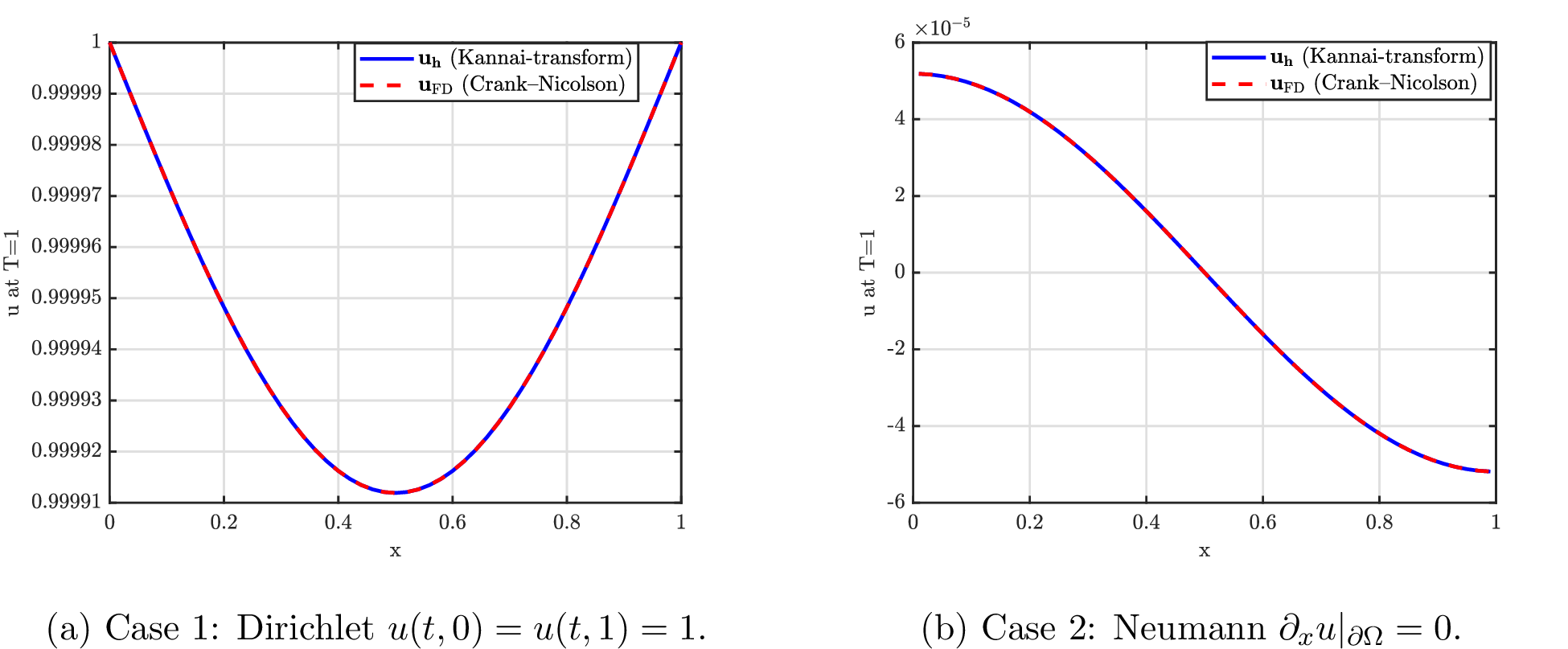
9 Conclusion↩︎
We developed a transmutation-based quantum framework for dissipative dynamics with factorized generators \(A=L^\dagger L\). By exploiting the Gaussian Kannai kernel, the method achieves improved query complexity with square-root dependence on \(T\|A\|\) and only polylogarithmic dependence on the target accuracy, up to the standard state-preparation and output-norm factors. We illustrated the framework for representative parabolic PDEs and showed that, in the long-time regime under a spectral-gap assumption, it also yields a structured quantum linear solver. This advantage is tied to the factorized access model, compatibility with the Gaussian Kannai transmutation, and favorable output norms; otherwise it may be reduced. Future work includes quantum preconditioning and extensions to time-dependent and more general non-self-adjoint operators.
Acknowledgments↩︎
SJ acknowledges the support of the NSFC grant No. 12341104, the Shanghai Pilot Program for Basic Research, the Science and Technology Commission of Shanghai Municipality (STCSM) grant no. 24LZ1401200, the Shanghai Jiao Tong University 2030 Initiative, and the Fundamental Research Funds for the Central Universities. CM was supported by Fundamental and Interdisciplinary Disciplines Breakthrough Plan of the Ministry of Education of China (JYB2025XDXM112) and NSFC grant No. 12501607. CM was also partially supported by the Science and Technology Commission of Shanghai Municipality (No.22DZ2229014). EZ was funded by the Alexander von Humboldt-Professorship program, the ERC Advanced Grant CoDeFeL, the Grant PID2023-146872OB-I00-DyCMaMod of MICIU (Spain), the COST Actions CA24136 - InterCoML and CA24122–mSPACE, supported by COST (European Cooperation in Science and Technology), the AFOSR 24IOE027 project, and the SURE-AI Centre grant 357482, Research Council of Norway.